Review of computational methods for estimating cell potency from single-cell RNA-seq data, with a detailed analysis of discrepancies between method description and code implementation

Abstract

In single-cell RNA sequencing (scRNA-seq) data analysis, a critical challenge is to infer hidden dynamic cellular processes from measured static cell snapshots. To tackle this challenge, many computational methods have been developed from distinct perspectives. Besides the common perspectives of inferring trajectories (or pseudotime) and RNA velocity, another important perspective is to estimate the differentiation potential of cells, which is commonly referred to as “cell potency.” In this review, we provide a comprehensive summary of $11$ computational methods that estimate cell potency from scRNA-seq data under different assumptions, some of which are even conceptually contradictory. We divide these methods into three categories: mean-based, entropy-based, and correlation-based methods, depending on how a method summarizes gene expression levels of a cell or cell type into a potency measure. Our review focuses on the key similarities and differences of the methods within each category and between the categories, providing a high-level intuition of each method. Moreover, we use a unified set of mathematical notations to detail the $11$ methods’ methodologies and summarize their usage complexities, including the number of ad-hoc parameters, the number of required inputs, and the existence of discrepancies between the method description in publications and the method implementation in software packages. Realizing the conceptual contradictions of existing methods and the difficulty for fair benchmarking without single-cell-level ground truths, we conclude that accurate estimation of cell potency from scRNA-seq data remains an open challenge.

Introduction

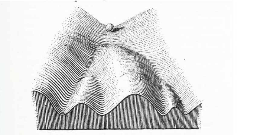
Figure 1: Waddington’s landscape [1]. This ball symbolizes a cell undergoing a differentiation process, while the valleys symbolize possible differentiation trajectories. As the ball descends the hill, it selects a specific pathway and eventually rests at the bottom of the hill, representing a differentiated cell that reaches its stable state.

In 1957, Conrad Hal Waddington drew a landscape (Figure 1) to depict the dynamic process of cell differentiation [1]. The drawing shows a ball placed on the top of an inclined hill with multiple valleys separated by ridges. The ball represents a cell in a differentiation process, while the valleys represent differentiation pathways. As the ball rolls down the hill, it follows one of the pathways and settles at the bottom of the hill, which represents the stable state of a differentiated cell. With the rapid advancement of technologies over the past $60$ years, we now have various means to quantify the dynamic process of cell differentiation.

The development of single-cell RNA sequencing (scRNA-seq) enabled researchers to profile gene expression at an unprecedentedly single-cell resolution. However, scRNA-seq provides solely a static snapshot of individual cells, rather than the underlying dynamic process of cell differentiation, if one exists. To infer the dynamic process from static scRNA-seq data, many computational methods have been developed, including the methods that estimate cell pseudotime (also known as trajectory inference) [2], RNA velocity [3], or cell potency.

Cell potency, also known as stemness, is a quantitative measure that indicates the differentiation capacity of a cell [4]. Two major differences exist between cell potency estimation and pseudotime or RNA velocity estimation. First, cell potency estimation is specific to the cell differentiation process, while pseudotime or RNA velocity estimation applies to other dynamic cellular processes, such as immune responses. Second, the estimated cell potency values indicate the direction of cell differentiation, while pseudotime estimation usually requires users to specify the starting point of a dynamic cellular process.

Ideally, cell potency estimation methods should assign the highest potency to stem cells and the lowest potency to fully differentiated cells. The accurate estimation of cell potency should reveal the hidden differentiation status of individual cells, thus expanding the capacity of scRNA-seq data analysis. Given the importance and abundance of cell potency estimation methods, in this review, we summarized and compared $11$ methods from multiple perspectives, including the measure and resolution of cell potency, the input data, as well as the incorporation of external information such as gene ontology (GO) and protein-protein interactions (PPIs).

Here we reviewed $11$ published computational methods for estimating cell potency from scRNA-seq data, including CytoTRACE [5], NCG [6], stemID [7], SLICE [8], dpath [9], scEnergy [10], SCENT [11], MCE [12], SPIDE [13], mRNAsi [14], and CCAT [15]. Tables 1 and 2 summarize the $11$ methods’ characteristics and high-level intuitions, respectively.

Due to the similar assumptions and approaches shared by some methods, we categorized the $11$ methods into three categories, including two mean-based methods (CytoTRACE and NCG), seven entropy-based methods (stemID, SLICE, dpath, scEnergy, SCENT, MCE, and SPIDE), and two correlation-based methods (mRNAsi and CCAT). As an overview, mean-based methods summarize a subset of genes’ expression levels into a mean-like statistic to represent a cell’s potency; entropy-based methods define an entropy-like measure to describe the expression level distribution of genes or gene groups in a cell; and correlation-based methods use externally defined gene importance scores to calculate a correlation between the scores and each cell’s gene expression levels.

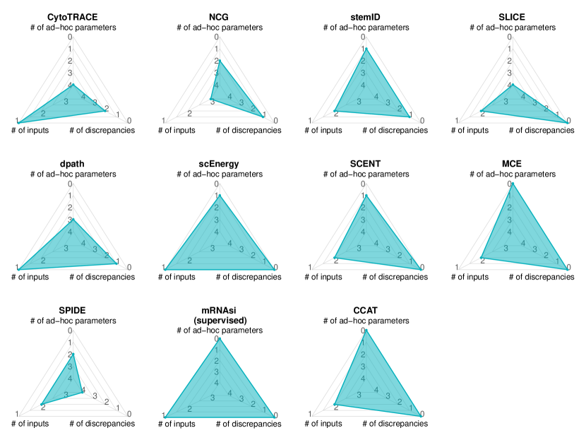
Figure 3: A radar plot for the $11$ cell potency estimation methods with respect to their number of inputs, number of ad-hoc parameters, and the number of discrepancies between their publication and code implementations, which can reflect the simplicity (number of inputs and ad-hoc parameters) and the consistency (number of discrepancies) of the methods.

During our detailed review of these methods, we spotted discrepancies between several methods’ descriptions in their publications and their code implementations in the corresponding software packages/scripts, whose version numbers or latest update dates when accessed (if the version number is unavailable) are listed in Table 3. We summarized these discrepancies in Table 4. We also noticed that some methods use ad-hoc parameters, and we summarized them in Table 5. In Figure 3, we used radar plots to compare the $11$ methods’ complexities in three dimensions: number of ad-hoc parameters, number of inputs, and number of discrepancies.

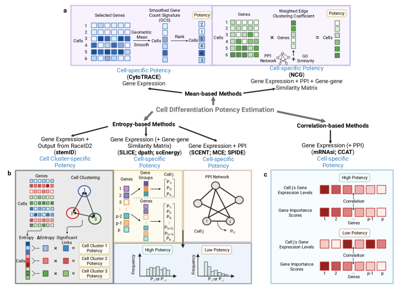
Figure 2: A conceptual categorization of the $11$ methods into three categories: mean-based methods, entropy-based methods, and correlation-based methods. All methods except stemID calculate the potency at the single-cell resolution, while stemID offers the cell-cluster resolution only. a) Mean-based methods. The CytoTACE method (left) computes a Gene Count Signature (GCS) for each cell using the selected genes only. Then CytoTRACE defines cells’ potency as the ranks of the cells’ smoothed GCS values. The NCG method (right) defines a weight for every gene by aggregating the gene’s similarities to other genes, and the gene-gene similarities are defined based on the genes’ edge weights in a PPI network and the genes’ GO terms. Then NCG uses the defined gene weights and a gene-by-cell log normalized expression matrix to estimate every cell’s potency. b) Entropy-based methods. These seven methods use entropy to define the potency and can be divided into three subcategories. In the first subcategory, stemID defines the potency of each cell cluster, not each cell, as the product of the cell cluster’s relative entropy ($\Delta\text{Entropy}$) and links (similarities) to other cell clusters. In the second subcategory, SLICE, dpath, and scEnergy first calculate a proportion vector $P_{\cdot j}$ for each cell $j$, where $P_{ij}$ is the proportion (i.e., the relative expression level) of gene group $i$ (SLICE and dpath) or gene $i$ (scEnergy) in cell $j$, and then define cell $j$’s potency as the entropy of $P_{\cdot j}$. Among the three methods in the second sub-category, SLICE requires users to input a gene-gene similarity matrix (the Kappa statistics for all gene pairs) while the other two methods does not. In the third subcategory, SCENT, MCE, and SPIDE define cell $j$’s potency as the entropy of a transition probability matrix (or extended vector) $P_{\cdot\cdot j}$, where $P_{ii^{\prime}j}$ is the transition probability (i.e., the normalized edge weight) from gene $i$ to gene $i^{\prime}$ in cell $j$. c) Correlation-based methods. The CCAT and mRNAsi methods define a cell’s potency as the correlation between the cell’s gene expression vector and a vector of pre-defined, non-cell-specific gene important scores. In CCAT, genes’ importance scores are the genes’ degrees in a PPI network; in mRNAsi, genes’ importance scores are the genes’ coefficients in a pre-trained one-class logistic regression model for predicting the probability that a given cell is a stem cell. CCAT requires users to input a PPI netweork while mRNAsi does not. (The figure was created with BioRender.com.)

In the following sections, we will introduce mathematical notations to unify the notations used in these $11$ methods, summarize these methods into the three categories: mean-based methods, entropy-based methods, and correlation-based methods (illustrated in Figure 2), and provide a detailed explanation for each method.

Unified mathematical notations

Before describing the $11$ methods, we introduce the following mathematical notations to unify the notations used in different methods and facilitate our discussion.

• $X\in\mathbb{Z}_{\geq 0}^{p\times n}$: a gene-by-cell count matrix, assuming we have $p$ genes and $n$ cells. The $(i,j)$-th entry $X_{ij}$ indicates the read or UMI (unique molecular identifier) count, which represents the measured expression level, of gene $i$ in cell $j$. The $j$-th column $X_{\cdot j}$ is a $p$-dimensional column vector consisting of all $p$ genes’ counts in cell $j$.

• $S\in\mathbb{R}_{\geq 0}^{p\times n}$: a gene-by-cell normalized expression matrix, in which the cell library size is normalized out. The $(i,j)$-th entry $S_{ij}$ is the normalized expression level of gene $i$ in cell $j$. Note that the purpose of normalization is to make gene expression levels comparable across cells, and different methods may use different normalization approaches.

• $Z\in\mathbb{R}_{\geq 0}^{p\times n}$: a gene-by-cell log normalized expression matrix (i.e., applying log transformation on $S$). The $(i,j)$-th entry $Z_{ij}$ is the log normalized expression level of gene $i$ in cell $j$. Note that different methods may use different log-normalizing approaches. The $j$-th column $Z_{\cdot j}$ is a $p$-dimensional column vector consisting of all $p$ genes’ log normalized expression levels in cell $j$.

• $A\in\{0,1\}^{p\times p}$: a gene-by-gene binary adjacency matrix from a user-inputted PPI network. $A$ is symmetric. For $i\neq i^{\prime}$, the $(i,i^{\prime})$-th entry $A_{ii^{\prime}}=1$ means that an edge exists between genes $i$ and $i^{\prime}$ in the PPI network, and $A_{ii^{\prime}}=0$ means otherwise. Note that $A_{ii}=0$ in SCENT and SPIDE, but $A_{ii}=1$ in MCE.

• $N(i)$: a set of gene $i$’s neighboring genes in the PPI network (i.e., the genes that have edges connecting with gene $i$). The size of $N(i)$ is $\sum_{i^{\prime}=1}^{p}A_{ii^{\prime}}$.

• $\Pi\in[0,1]^{p\times n}$: a gene-by-cell steady-state probability matrix. The $(i,j)$-th entry $\Pi_{ij}$, defined based on $X_{ij}$, $S_{ij}$, or $Z_{ij}$ (different methods may have different definitions), represents the steady-state probability of gene $i$ in cell $j$. Intuitively, $\Pi_{ij}$ serves as a weight for gene $i$ in cell $j$. For SCENT and SPIDE, if we fix the total expression level of gene $i$’s neighboring genes in cell $j$, i.e., $\sum_{i^{\prime}\in N(i)}Z_{i^{\prime}j}$, then $\Pi_{ij}$ increases with $Z_{ij}$; if we fix $Z_{ij}$, then $\Pi_{ij}$ increases with $\sum_{i^{\prime}\in N(i)}Z_{i^{\prime}j}$. For MCE, $\Pi_{ij}=S_{ij}:=X_{ij}/\left(\sum_{i^{\prime}=1}^{p}X_{i^{\prime}j}\right)$ and thus increases with $S_{ij}$.

• $R_{j}\in[-1,1]^{p\times p}$: a gene-by-gene correlation matrix of cell $j$. The $(i,i^{\prime})$-th entry $R_{ii^{\prime}j}$ is the Pearson correlation calculated based on

  $$\{(Z_{ij^{\prime}},Z_{i^{\prime}j^{\prime}}):\text{cell }j^{\prime}\text{ is among the $K$ nearest neighbors of cell }j\}\,.$$

  Specifically, each cell $j$’s $K$ nearest neighbors are defined based on the Pearson correlation applied to $Z$, i.e., the distance between cells $j$ and $j^{\prime}$ is $1-\text{cor}(Z_{\cdot j}\,{,}\,Z_{\cdot j^{\prime}})$.

• $P_{j}\in[0,1]^{p\times p}$: a gene-by-gene transition probability matrix of cell $j$. The $(i,i^{\prime})$-th entry $P_{ii^{\prime}j}$ represents the transition probability from gene $i$ to gene $i^{\prime}\in N(i)$ in cell $j$. This transition probability is defined as an aggregation of the gene expression and PPI information, including $Z_{ij}$, $\{Z_{i^{\prime}j}:i^{\prime}\in N(i)\}$, as well as $R_{ii^{\prime}j}$. Different methods may aggregate these sources of information in different ways.

• $W_{j}\in\mathbb{R}_{\geq 0}^{p\times p}$: a gene-by-gene edge weight matrix of cell $j$. The $(i,i^{\prime})$-th entry $W_{ii^{\prime}j}$ represents the edge weight between gene $i$ and gene $i^{\prime}\in N(i)$. $W_{ii^{\prime}j}$ is defined based on $Z_{ij}$, $Z_{i^{\prime}j}$ and $R_{ii^{\prime}j}$, and different methods may have different definitions.

• $E_{j}$: the entropy for cell $j$ calculated by an entropy-based method.

• $\mathrm{\it{NE}}_{j}$: the normalized entropy for cell $j$ ($E_{j}$ is normalized by a constant $C$; the definition of $C$ differs across entropy-based methods).

Category 1: mean-based methods

Referred to as mean-based methods, CytoTRACE [5] and NCG [6] both summarize a cell’s gene expression levels into a mean-based summary statistic to represent the cell’s potency.

CytoTRACE

CytoTRACE [5] relies on the assumption that a cell’s gene count (i.e., the number of expressed genes) reflects the cell’s differentiation status. Accordingly, CytoTRACE first selects the genes whose expression levels highly correlate with the gene count across cells. Then CytoTRACE defines the gene count signature (GCS) as the geometric mean of the selected genes’ expression levels in each cell. Finally, CytoTRACE performs smoothing on the cells’ GCSs and then converts the smoothed GCSs into ranks, which serve as the final estimates of the cells’ potency.

Technically, CytoTRACE first transforms $X\in\mathbb{Z}_{\geq 0}^{p\times n}$ to CPM $S\in\mathbb{R}_{\geq 0}^{p\times n}$ (Count Per Million; $S_{ij}=X_{ij}/\sum_{i^{\prime}=1}^{p}X_{ij}\times 10^{6}$) and then to $Z\in\mathbb{R}_{\geq 0}^{p\times n}$, with $Z_{ij}=\log_{2}\left(C_{j}\frac{S_{ij}}{\sum_{i^{\prime}=1}^{p}S{i^{\prime}j}}+1\right)$, where $C_{j}=\sum_{i^{\prime}=1}^{p}\mathbb{I}(X_{i^{\prime}j}>0)$ is cell $j$’s gene count. Second, CytoTRACE calculates the Pearson correlation between all $n$ cells’ gene counts $(C_{1},C_{2},\ldots,C_{n})^{\mkern-1.5mu\mathsf{T}}$ and gene $i$’s log normalized expression levels in the $n$ cells $(Z_{i1},Z_{i2},\ldots,Z_{in})^{\mkern-1.5mu\mathsf{T}}$, for each gene $i=1,\ldots,p$. Third, CytoTRACE selects the top $200$ genes that have the highest correlation values to compute the GCS for each cell, obtaining $G=(G_{1},G_{2},\ldots,G_{n})^{\mkern-1.5mu\mathsf{T}}\in\mathbb{R}_{\geq 0}^{n}$, where $G_{j}$ is cell $j$’s GCS, defined as the geometric mean of the $200$ genes’ log normalized expression levels in cell $j$. However, the GCS is defined as the arithmetic mean instead in the code implementation, different from the publication. Fourth, CytoTRACE performs smoothing on $G$ by taking the following sub-steps.

1. Filter the rows of $Z$ to retain only the genes that are expressed in at least $5\%$ of the $n$ cells. For each retained gene $i$, compute a dispersion index as the gene’s variance over its mean across the $n$ cells, i.e., $\frac{1}{n-1}\sum_{j=1}^{n}(Z_{ij}-\bar{Z}_{i})^{2}/\bar{Z}_{i}$, where $\bar{Z}_{i}=\frac{1}{n}\sum_{j=1}^{n}Z_{ij}$. Further, filter the rows of $Z$ to retain only the $1{,}000$ genes with the largest dispersion indices. Hence, the dimension of $Z$ becomes $1{,}000\times n$.

   We note that this gene selection sub-step is performed before the second step above in the code implementation, and the selected $1{,}000$ genes are used to select $\tilde{n}$ cells (see footnote), creating a discrepancy between the code implementation and the publication. Specifically, in the second step above, each Pearson correlation is calculated across all $n$ cells in the publication but only the $\tilde{n}$ cells in the code implementation. Hence, the top $200$ genes selected in the third step above differ between the code implementation and the publication. Also, the dimension of $Z$ in the code becomes $1{,}000\times\tilde{n}$. Thus, in the following sub-steps, the cell number $n$ becomes $\tilde{n}$ in the code.

2. Obtain a cell-by-cell Markov matrix $B\in[-1,1]^{n\times n}$ in two steps.

   1. Compute a cell-by-cell similarity matrix $D\in[-1,1]^{n\times n}$, in which $D_{jj^{\prime}}$ is the Pearson correlation between cell $j$ and cell $j^{\prime}$ based on the retained $1{,}000$ genes’ expression levels in $Z$, i.e., the Pearson correlation between the two columns $Z_{\cdot j}$ and $Z_{\cdot j^{\prime}}$.

   2. Transform $D$ to $B$ as

      $$B_{jj^{\prime}}=\left\{\begin{array}[]{ll}0&\text{if }j=j^{\prime}\text{ or }D_{jj^{\prime}}<\tau\\ D_{jj^{\prime}}&\text{otherwise}\end{array}\right.\,,$$

      where $\tau=\frac{1}{n^{2}}\sum_{j=1}^{n}\sum_{j^{\prime}=1}^{n}D_{jj^{\prime}}$ is the mean of $D$.

3. Transform $G$ to $G_{0}\in\mathbb{R}_{\geq 0}^{n}$ using non-negative least squares regression, which finds an $n$-dimensional vector $\beta_{0}=\operatorname*{arg\,min}_{\beta\geq 0}\|G-B\beta\|_{2}^{2}$, and defining $G_{0}=B\beta_{0}$.

4. Simulate a diffusion process for $T=10{,}000$ iterations or until convergence:

   $$G_{t+1}=\alpha\cdot BG_{t}+(1-\alpha)\cdot G_{0}\,;\;t=0,\ldots,T-1\,,$$

   where the degree of diffusion $\alpha=0.9$.

Finally, CytoTRACE estimates the potency by converting the $n$ values in $G_{T}\in\mathbb{R}_{\geq 0}^{n}$ from the last iteration into ranks $n$ to $1$ (with $n$ indicating the maximum value in $G_{T}$).

The intuition behind CytoTRACE is that a cell has a higher potency if it has more genes expressed.

Compared with the other $10$ methods, CytoTRACE has one of the most complicated procedures. The ad-hoc parameters in CytoTRACE include the two gene numbers ($200$ and $1{,}000$) used to calculate $G$ and $D$ respectively, the percentage threshold used to filter out genes of $5\%$, as well as the degree of diffusion $\alpha$ in the diffusion process. In total, we count CytoTRACE to have four ad-hoc parameters.

NCG

NCG [6] defines cell potency from scRNA-seq data, a PPI network, and GO annotations. First, NCG performs quantile normalization on the inputted count matrix $X=(X_{ij})$ to obtain $S=(S_{ij})$. Then, NCG log transforms $S$ to obtain $Z=(Z_{ij})$. In the publication, if $S_{ij}<1$, $Z_{ij}=\log_{2}(S_{ij}+1.1)$; otherwise, $Z_{ij}=\log_{2}(S_{ij}+0.1)$ (Noted that in NCG’s code implementation, $Z_{ij}$ is always $\log_{2}(S_{ij}+0.1)$; if $S_{ij}<1$, then $S_{ij}$ is set to $1$, and $Z_{ij}$ becomes a constant $\log_{2}1.1$, which we find unreasonable). Next, NCG defines a weighted edge clustering coefficient of the gene (ECG) for each gene in both the scRNA-seq data and the PPI network. The ECG for gene $i$ is $\mathrm{\it{ECG}}_{i}=\sum_{i^{\prime}=1}^{p}w_{ii^{\prime}}\times\mathrm{\it{ECC}}_{ii^{\prime}}$, in which $p$ is the number of genes in both the scRNA-seq data and the PPI network, $w_{ii^{\prime}}$ is the similarity between gene $i$ and gene $i^{\prime}$ defined as the Kappa statistic applied to the two genes’ GO annotations (detailed below), and $\mathrm{\it{ECC}}_{ii^{\prime}}$ is the edge clustering coefficient (ECC) (defined as $|N(i)\cap N(i^{\prime})|/(\min(N(i),N(i^{\prime}))-1)$, the number of common neighbors between gene $i$ and gene $i^{\prime}$ divide by the minimum degree of the two genes minus $1$; it is set to $0$ when the denominator is $0$). Note that the ECC measures the degree of closeness of two genes in a PPI network. Intuitively, if a gene has a higher ECG value, it is similar to more genes based on the PPI network and GO annotations.

Next, NCG computes the potency for cell $j$ as

$$\mathrm{\it{NCG}}_{j}=\frac{1}{\max_{j^{\prime}\in\{1,\cdots,n\}}\mathrm{\it{NCG}}_{j^{\prime}}}\sum_{i=1}^{p}Z_{ij}\times\mathrm{\it{ECG}}_{i}\,.$$

A high value of $\mathrm{\it{NCG}}_{j}$ indicates a high potency value of cell $j$.

Since the Kappa statistic for each gene pair is a required input that users must specify, the NCG paper [6] does not detail the calculation of the Kappa statistic. Based on literature [16, 17], the Kappa statistic $w_{ii^{\prime}}$ between gene $i$ and gene $i^{\prime}$ is defined as follows. Given a total of $N$ GO terms, we could construct the following confusion matrix based on the two genes’ GO terms.

Gene $i^{\prime}$
Gene $i$		$1$	$0$	Row Total
	$1$	$N_{ii^{\prime}}^{11}$	$N_{ii^{\prime}}^{10}$	$N_{i\cdot}^{1*}$
	$0$	$N_{ii^{\prime}}^{01}$	$N_{ii^{\prime}}^{00}$	$N_{i\cdot}^{0*}$
	Column Total	$N_{\cdot i^{\prime}}^{*1}$	$N_{\cdot i^{\prime}}^{*0}$	${N}$

In the confusion matrix, we divide the $N$ GO terms based on whether they belong to gene $i$ and/or gene $i^{\prime}$, with the row or column label of $1$ indicating belonging and $0$ otherwise. Then for example, $N_{ii^{\prime}}^{11}$ indicates the number of GO terms shared by genes $i$ and $i^{\prime}$, and $N_{ii^{\prime}}^{10}$ means the number of GO terms belonging to gene $i$ but not to gene $i^{\prime}$. The Kappa statistic is then defined as $w_{ii^{\prime}}=\frac{O_{ii^{\prime}}-E_{ii^{\prime}}}{1-E_{ii^{\prime}}}$ where $O_{ii^{\prime}}=\frac{N_{ii^{\prime}}^{11}+N_{ii^{\prime}}^{00}}{N}$ and $E_{ii^{\prime}}=\frac{N_{i\cdot}^{1*}N_{i\cdot}^{*1}+N_{\cdot i^{\prime}}^{0*}N_{\cdot i^{\prime}}^{*0}}{N^{2}}$.

The intuition behind NCG is that, with a subset of genes identified as closely connected in the PPI network and sharing similar GO terms, a cell has a higher potency if the identified genes have higher expression in it.

The ad-hoc parameters in NCG include the offset $1.1$ used in the log transformation ($Z_{ij}=\log_{2}(S_{ij}+\text{offset})$) and the cutoff value of $1$ for $S_{ij}$ to decide which offset value ($1.1$ or $0.1$) to use. We do not count the other offset $0.1$ used for $S_{ij}\geq 1$ as an ad-hoc parameter because we interpret this offset value to make $Z_{ij}$ continuous at $S_{ij}=1$ in the code implementation (however, this interpretation does not hold for the publication, which differs from the code implementation). In total, we count NCG to have two ad-hoc parameters.

Category 2: entropy-based methods

Out of the $11$ methods, seven methods (stemID [7], SLICE [8], dpath [9], scEnergy [10], SCENT [11], MCE [12], and SPIDE [13]) use various ways to define and calculate the entropy, i.e., the cell potency measure, of each cell or cell cluster. These methods are based on the rationale that stem cells should have higher entropy values (i.e., gene expression levels have a more uniform distribution), while mature cells should have lower entropy values (i.e., gene expression levels have a less uniform distribution, such as a bimodal distribution).

Based on the methodological details, we further separate the seven methods into three sub-categories. The first sub-category only includes stemID, which first finds cell clusters, and then uses clusters’ similarities and relative gene expression levels to calculate an entropy for each cluster. stemID is the only method that does not estimate potency at a single-cell resolution. The second sub-category includes SLICE, dpath, and scEnergy, which use the relative or binarized expression levels of either gene groups or individual genes to estimate the potency of each cell. The third sub-category includes SCENT, MCE, and SPIDE, which use different ways to define genes’ steady-state probabilities and gene-to-gene transition probabilities based on a PPI network and gene expression levels. Then, they aggregate these probabilities into an entropy-like measure for each cell. Finally, they normalize the measure as a potency estimate for each cell.

stemID

Among the seven entropy-based methods, stemID [7] is the only one that estimates the potency of cell clusters instead of cells. Hence, stemID requires users to run the clustering method RaceID2 [7], which was developed by the same authors. The RaceID2 result contains each cell’s cluster label and each cluster’s medoid.

First, stemID links all pairs of cluster medoids and determines the significance of each link as follows: every cell is projected to the closest link (by vertical distance in the embedding space by multi-dimensional scaling, which preserves the pairwise cell distances) among the links that connect the cell’s cluster medoid to other cluster medoids; after all cells are projected, each link has its projected cells, whose number would then be converted to a p-value (considered significant if under a default significance level of $0.01$). Given the significant links, stemID computes the number of significant links involving each cluster $k$’s medoid and denotes the number as $l_{k}$.

Next, stemID computes the entropy value of cell $j$ as $E_{j}=-\sum_{i=1}^{p}S_{ij}\log_{p}S_{ij}$ (note that the negative sign was missing in the original article as a typo), where $S_{ij}:=X_{ij}/\sum_{i^{\prime}=1}^{p}X_{i^{\prime}j}$ is the proportion of gene $i$’s expression level in cell $j$.

Finally, stemID computes a stemness score $s_{k}$ as the estimated potency for each cell cluster $k$ as

$$s_{k}=l_{k}\times\Delta E_{k}\,,$$

where $\Delta E_{k}$ is the difference between cluster $k$’s median cell entropy value (i.e., the median of the entropy values of the cells in cluster $k$) and the minimum of all clusters’ median cell entropy values.

The intuition behind stemID is that a cluster has a higher potency if it has more clusters in proximity and contains more cells with more uniform gene expression levels.

The ad-hoc parameter in stemID is the significance level of $0.01$ used for identifying significant links. In total, we count stemID to have one ad-hoc parameter.

Unlike stemID, the other six entropy-based methods estimate the potency of each cell.

SLICE

SLICE [8] defines the potency measure, called scEntropy, for each cell based on the inputted gene expression matrix (which can be on the scale of FPKM (Fragments Per Kilobase of transcript per Million mapped reads), RPKM (Reads Per Kilobase per Million mapped reads), or TPM (Transcripts Per Million)) and GO annotations. Specifically, SLICE calculates a cell-specific entropy based on gene groups instead of genes, unlike stemID; SLICE clusters genes into groups by performing $k$-means clustering on a gene-gene dissimilarity matrix, which the gene-gene dissimilarities are measured by one minus the Kappa statistic applied to the genes’ GO terms (same as the Kappa statistic used in NCG), and this Kappa statistic matrix is a required user input. SLICE’s R package provides the similarity matrices measured by Kappa statistics for human genes and mouse genes, respectively.

Note that the default use of the $k$-means clustering might be problematic because the $k$-means clustering should be a gene-by-feature matrix instead of SLICE’s symmetric gene-gene dissimilarity matrix.

In detail, for each cell $j$, SLICE computes the scEntropy as

$$E_{j}=\frac{1}{B}\sum_{b=1}^{B}\sum_{m=1}^{M}-p_{j}^{m}(G_{b},F_{b})\log p_{j}^{m}(G_{b},F_{b})\,,$$

where $G_{b}$ is a random subsample of $p_{s}=1{,}000$ genes with expression levels greater than $1$ in at least one cell (note that the original article incorrectly referred to $G_{b}$ as a “bootstrap sample”), $F_{b}$ denotes the $M=\sqrt{p_{s}/2}=22$ gene groups clustered from the genes in $G_{b}$, and $p_{j}^{m}(G_{b},F_{b})=\frac{c_{j}^{m}(G_{b},F_{b})+\alpha^{m}}{C_{j}(G_{b},F_{b})+A}$, in which $c_{j}^{m}(G_{b},F_{b})$ denotes the number of genes in $G_{b}$ expressed in cell $j$ and belonging to the $m$-th group in $F_{b}$, $\alpha^{m}$ denotes the proportion of genes in $G_{b}$ belonging to the $m$-th group in $F_{b}$ (i.e. the number of genes in $G_{b}$ belonging to he $m$-th group in $F_{b}$ divided by $p_{s}$), $C_{j}(G_{b},F_{b})=\sum_{m=1}^{M}c_{j}^{m}(G_{b},F_{b})$, and $A=\sum_{m=1}^{M}\alpha^{m}$. Hence, $p_{j}^{m}(G_{b},F_{b})$ measures the relative degree of activeness (i.e., proportion) of the $m$-th gene group in $F_{b}$ in cell $j$, and $E_{j}$ denotes cell $j$’s average entropy calculated on the proportions of $M$ gene groups across $B=100$ subsamples. SLICE outputs $E_{j}$ as the estimated potency for cell $j$. Here, the values of $M$ and $B$ are from SLICE’s tutorials [18].

Note that SLICE treats gene expression counts as binary because it only considers if a gene is expressed or not in a cell in its scEntropy calculation.

The intuition behind SLICE is that a cell has a higher potency if its binarized gene expression levels are more uniformly distributed. However, the uniform distribution is defined based on $M$ gene groups, whose definition changes across gene subsamples.

The ad-hoc parameters in SLICE include the expression level threshold of $1$ used to filter out genes, the number of genes in each subsample ($p_{s}$), the number of gene groups ($M$), and the number of subsamples ($B$). In total, we count SLICE to have four ad-hoc parameters.

dpath

dpath [9] is similar to SLICE but uses a different way to partition genes into groups: dpath first log-transforms the inputted gene-by-cell TPM matrix to obtain $Z$ ($Z=\log(\text{TPM}+1)$). Then, dpath performs a weighted non-negative factorization (NMF) on $Z$ to cluster genes into $M$ (default $5$) groups (called “metagenes”). The factorization is in the form of $Z\approx UV$, where $U$ is a gene-by-metagene non-negative matrix, and $V$ is a metagene-by-cell non-negative matrix satisfying $\sum_{m=1}^{M}V_{mj}=1$ for all cell $j$ (i.e., every column of $V$ sums up to $1$, so $V_{mj}$ indicates the proportion of metagene $m$ in cell $j$). The dpath authors denoted $\mu=(\mu_{ij})=UV$ as the expected gene-by-cell logTPM matrix. Given the observed gene-by-cell logTPM matrix $Z$, the dpath authors wrote the log-likelihood of $U$, $V$, and $\pi$ (a gene-by-cell weight matrix as a parameter to be estimated) as

$$\ell(U,V,\pi)=\sum_{i=1}^{p}\sum_{j=1}^{n}\left[\pi_{ij}\cdot\log\text{Poisson}(Z_{ij}~{}|~{}\mu_{ij})\right.\left.+~{}(1-\pi_{ij})\cdot\log\text{Poisson}(Z_{ij}~{}|~{}0.1)\right]\,,$$

where $\text{Poisson}(\cdot|\lambda)$ represents the probability mass function of the Poisson distribution with mean $\lambda$; $\pi_{ij}$ is the weight for gene $i$ in cell $j$; $\mu_{ij}$ is the expected logTPM of gene $i$ in cell $j$; and $0.1$ is the mean parameter of the Poisson distribution that models the dropout events. However, we did not find it appropriate to use the Poisson distribution to model logTPM data.

Then dpath estimates $U$, $V$, and $\pi$ through an iterative optimization process to maximize the log-likelihood $\ell(U,V,\pi)$, and this process is referred to as the “weighted NMF.” In detail, dpath performs two rounds of interations in the optimization process. First, dpath iteratively solves $U$ and $V$ by fixing $\pi$ across all iterations: $\pi_{ij}=1$ if $Z_{ij}>0$, and $\pi_{ij}=0.1$ otherwise (note that in the dpath package, $\pi_{ij}$ was set to $0$ instead of $0.1$, the value written in the dpath paper); hence, non-zero $Z_{ij}$’s have larger weights than zero $Z_{ij}$’s. Second, dpath uses the $U$ and $V$ found by the first round of iterations as the initialization and iteratively solves $U$, $V$ and $\pi$; in the $t$-th iteration of the second round, $\pi_{ij}$ is updated as $\pi_{ij}^{t}=\frac{\text{Poisson}(Z_{ij}~{}|~{}\mu_{ij}^{t})}{\text{Poisson}(Z_{ij}~{}|~{}\mu_{ij}^{t})~{}+~{}\text{Poisson}(Z_{ij}~{}|~{}0.1)}$, where $\mu_{ij}^{t}=\sum_{m=1}^{M}U_{im}^{t}V_{mj}^{t}$.

Using $V$ outputted by the second round, dpath estimates the potency for cell $j$ as

$$E_{j}=-\sum_{m=1}^{M}V_{mj}\log V_{mj}\,.$$

The intuition behind dpath is that a cell has a higher potency if its metagene expression levels are more uniformly distributed.

The ad-hoc parameters in dpath include the number of metagenes ($M$), the mean parameter for the Poisson distribution that models the dropout event (default parameter value $0.1$), and the value of $\pi_{ij}=0.1$ used in the first round of the weighted NMF for $Z_{ij}=0$. In total, we count dpath to have three ad-hoc parameters.

scEnergy

scEnergy [10] is different from SLICE and dpath because it does not calculate the cell-specific entropy based on gene groups. Instead, scEnergy considers every gene and the neighboring genes in a gene network constructed from the inputted gene-by-cell expression matrix (which can be on the scale of TPM, FPKM, or UMI count). Specifically, scEnergy first constructs a gene network by connecting every two genes that have absolute Spearman correlations greater than a threshold (default $0.1$); a correlation is calculated based on two genes’ log-transformed counts ($\log_{2}(\text{count}+1)$) in all cells. Then for cell $j$, scEnergy defines the energy as

$$E_{j}=-\sum_{i=1}^{p}Z_{ij}\log\frac{Z_{ij}}{\sum_{i^{\prime}\in N(i)}{Z_{i^{\prime}j}}}\,,$$

where $Z_{ij}$ is the log normalized expression level for gene $i$ in cell $j$ (such that $\sum_{i}Z_{ij}=1$).

Finally, scEnergy estimates the potency for cell $j$ by re-scaling the energy $E_{j}$ as

$$\mathrm{\it NE}_{j}=\frac{(E_{j}/\overline{E})^{2}}{1+(E_{j}/\overline{E})^{2}}\,,$$

where $\overline{E}$ is the average energy of all cells, and $\mathrm{\it NE}_{j}$ is outputted as the estimated potency of cell $j$. However, we were unclear about the intuition behind the $E_{j}$ definition (which was claimed to be based on maximum entropy and statistical thermodynamics, but we could not find the exact connection) and the re-scaling, whose rationale was not mentioned in the scEnergy publication [10].

The rough intuition behind scEnergy is that a cell has a higher potency if its gene expression levels are more uniformly distributed.

The ad-hoc parameter in scEnergy is the threshold of $0.1$ for gene pairs’ absolute Spearman correlations when constructing the gene network. In total, we count scEnergy to have one ad-hoc parameter.

SCENT

SCENT [11] differs from stemID, SLICE, dpath, and scEnergy in the probabilities used for entropy calculation. Using the signaling entropy definition in the SCENT authors’ previous work [19, 20], SCENT takes as inputs (1) a log normalized gene-by-cell expression matrix $Z$, with the log normalized expression of gene $i$ in cell $j$ as $Z_{ij}=\log_{2}(S_{ij}+1.1)$, where $S_{ij}$ is $X_{ij}$ (the count of gene $i$ in cell $j$) multiplied by cell $j$’s specific scaling factor calculated externally and (2) a PPI network that specifies the gene-by-gene binary adjacency matrix $A\in\{0,1\}^{p\times p}$. Then for each cell $j$, SCENT calculates the signaling entropy as

$$E_{j}=-\sum_{i=1}^{p}\Pi_{ij}\sum_{i^{\prime}\in N(i)}P_{ii^{\prime}j}\log P_{ii^{\prime}j}\,.$$

The $E_{j}$ formula has two key components. First, the steady-state probability of gene $i$ in cell $j$ is

$$\Pi_{ij}=\frac{Z_{ij}(A\cdot Z_{\cdot j})_{i}}{Z_{\cdot j}^{\intercal}\cdot(A\cdot Z_{\cdot j})}\,,$$

where $Z_{\cdot j}\in\mathbb{R}_{\geq 0}^{p}$ is the log normalized gene expression vector of cell $j$, and $(A\cdot Z_{\cdot j})_{i}$ is the $i$-th element of the vector $(A\cdot Z_{\cdot j})\in\mathbb{R}_{\geq 0}^{p}$ and is equivalent to $\sum_{i^{\prime}\in N(i)}Z_{i^{\prime}j}$. Second, the transition probability from gene $i$ to gene $i^{\prime}$ in cell $j$ is

$$P_{ii^{\prime}j}=\frac{W_{ii^{\prime}j}}{\sum_{i^{\prime\prime}\in N(i)}W_{ii^{\prime\prime}j}}\,,$$

where $W_{ii^{\prime}j}=Z_{ij}Z_{i^{\prime}j}$, so $P_{ii^{\prime}j}=\frac{Z_{i^{\prime}j}}{\sum_{i^{\prime\prime}\in N(i)}Z_{i^{\prime\prime}j}}$ is irrelevant to $Z_{ij}$ and only uses gene $i$’s neighbors in the PPI network.

SCENT estimates the potency for each cell $j$ as

$$\mathrm{\it{NE}}_{j}=E_{j}/C\,,$$

in which the normalization constant $C$ is the maximum signaling entropy defined as

$$C=\max_{P=(P_{ii^{\prime}})}\left(-\sum_{i=1}^{p}\Pi_{ij}\sum_{i^{\prime}\in N(i)}P_{ii^{\prime}}\log P_{ii^{\prime}}\right)=-\sum_{i=1}^{p}\Pi_{ij}\sum_{i^{\prime}\in N(i)}\left(\frac{A_{ii^{\prime}}\nu_{i^{\prime}}}{\lambda\nu_{i}}\right)\log\left(\frac{A_{ii^{\prime}}\nu_{i^{\prime}}}{\lambda\nu_{i}}\right)=\log\lambda\,,$$

where $\lambda$ is the largest eigenvalue of the adjacency matrix $A$, and $\nu_{i}$ is the $i$-th element in the eigenvector $\nu$ corresponding to the largest eigenvalue. The last equality $C=\log\lambda$ was proven in [21].

As the number of cells increases, SCENT becomes computationally intensive. Therefore, CCAT, a faster proxy of SCENT, was proposed. Since CCAT’s approach does not involve entropy calculation, it belongs to another category we define as “correlation-based methods,” and we will discuss CCAT in the corresponding section.

The intuition behind SCENT is that a cell $j$ has a higher potency if its “influential” genes (i.e., gene $i$ is influential in cell $j$ if it has a large $\Pi_{ij}$, indicating gene $i$ is highly expressed in cell $j$ or has neighboring genes highly expressed in cell $j$) have neighboring genes’ expression levels more uniformly distributed.

The ad-hoc parameter in SCENT is the offset value of $1.1$ used in log transformation $Z_{ij}=\log_{2}(S_{ij}+\text{offset})$. In total, we count SCENT to have one ad-hoc parameter.

The last two entropy-based methods, MCE [12] and SPIDE [13], are similar to SCENT in that they all use genes’ expression levels and genes’ relationships in a PPI network to compute an entropy for each cell.

MCE

MCE (Markov Chain Entropy) defines the entropy for each cell $j$ as

$$E_{j}=\max_{P_{j}=(P_{ii^{\prime}j})\text{ s.t. }P_{j}\Pi_{\cdot j}=\Pi_{\cdot j}}\left(-\sum_{(i,i^{\prime})\in\hat{G}}\Pi_{ij}{P_{ii^{\prime}j}}\log(\Pi_{ij}P_{ii^{\prime}j})\right)\,,$$

where $(i,i^{\prime})$ indicates an edge between genes $i$ and $i^{\prime}$ in a PPI network, and $\hat{G}$ is a set including all edges in the PPI network, including all self-loop edges. In the above definition of $E_{j}$, $\Pi_{ij}=X_{ij}/(\sum_{i^{\prime}=1}^{p}X_{i^{\prime}j})$ is the steady-state probability of gene $i$ in cell $j$, and $\Pi_{\cdot j}$ is cell $j$’s steady-state probability vector; $P_{ii^{\prime}j}$ is the $(i,i^{\prime})$-th element in cell $j$’s transition matrix $P_{j}$ that satisfies $P_{j}\Pi_{\cdot j}=\Pi_{\cdot j}$ and $P_{j}\mathbf{1}=\mathbf{1}$. The computation of $E_{j}$ is solved as a convex optimization problem.

MCE’s final estimate of cell $j$’s potency is $\mathrm{\it{NE}}_{j}=E_{j}/C$, in which the normalization constant $C=\log(\sum_{i=1}^{p}d_{i})$, with $d_{i}$ representing the degree of gene $i$ in the PPI network.

Two major differences between MCE and SCENT are as follows. First, the inputted PPI network for MCE can have all ones on the diagonal of the adjacency matrix, while for SCENT the diagonal must have all zeros. Second, the transition probability matrix $P_{j}$ of cell $j$ is optimized given the steady-state probability $\Pi_{j}$ for MCE, while $P_{j}$ is computed based on the log normalized gene expression levels for SCENT.

The intuition behind MCE is that a cell has a higher potency if the weighted gene-to-gene transition probabilities in the PPI network are more uniformly distributed.

We count MCE to have zero ad-hoc parameters.

SPIDE

Similar to SCENT and MCE, SPIDE also defines an entropy for each cell using both gene expression levels and a PPI network. However, SPIDE uses a more complicated procedure to process gene expression levels. Since the notations in SPIDE’s publication are erroneous, the following description of SPIDE is based on our understanding of both the publication and code implementation. Specifically, SPIDE first performs imputation to reduce data sparsity. In the code implementation, for each cell $j$, SPIDE finds its $k$-nearest neighbors ($k=10$ for datasets with $1{,}000$ cells or fewer; $k=25$ for datasets with more than $1{,}000$ cells) as those cells with the highest Pearson correlations with cell $j$ based on the $\log_{2}(\text{count}+1.1)$ transformed expression levels (the count of gene $i$ in cell $j$ is $X_{ij}$). However, as illustrated in Figure 1 of SPIDE’s publication, SPIDE finds the $k$-nearest neighbors based on the cell-cell correlations calculated using log-transformed and quantile-normalized data, which is inconsistent with the code implementation. For each gene, if its raw count in cell $j$ is zero, then SPIDE computes two averages of the gene’s raw count—one across cell $j$’s $k$-nearest neighbors and the other across all cells. If the first average is no less than the second (in the publication; in the code, ”no less than” becomes ”greater than”), SPIDE replaces the gene’s zero expression level in cell $j$ with the first average. Then, SPIDE further processes the imputed data by quantile normalization and log transformation.

With the imputed and log normalized gene expression levels and the PPI network, SPIDE defines the entropy for cell $j$ as

$$E_{j}=-\sum_{i=1}^{p}\Pi_{ij}\sum_{i^{\prime}\in N(i)}P_{ii^{\prime}j}\log P_{ii^{\prime}j}\,,$$

which is exactly the same formula as SCENT’s signaling entropy.

Despite the same entropy formula, there are three differences between SPIDE and SCENT. First, the two methods use different definitions of $Z_{ij}$, the expression level of gene $i$ in cell $j$, which is used to define $P_{ii^{\prime}j}$, the transition probability from gene $i$ to gene $i^{\prime}$ in cell $j$. Recall that SCENT defines $Z_{ij}$ as a log normalized expression level, while SPIDE defines $Z_{ij}$ by imputation followed by quantile normalization and log transformation. Second, SPIDE changes the definition of $W_{ii^{\prime}j}$ in $P_{ii^{\prime}j}=\frac{W_{ii^{\prime}j}}{\sum_{i^{\prime\prime}\in N(i)}W_{ii^{\prime\prime}j}}$. Recall that in SCENT, $W_{ii^{\prime}j}=Z_{ij}Z_{i^{\prime}j}$, so $P_{ii^{\prime}j}=\frac{Z_{i^{\prime}j}}{\sum_{i^{\prime\prime}\in N(i)}Z_{i^{\prime\prime}j}}$. In contrast, SPIDE defines $W_{ii^{\prime}j}=\lvert R_{ii^{\prime}j}\lvert Z_{ij}Z_{i^{\prime}j}$, where $R_{ii^{\prime}j}$ the Pearson correlation between genes $i$ and $i^{\prime}$ based on the imputed, normalized, and log-transformed expression levels (in publication; in the code, $R_{ii^{\prime}j}$ is calculated using the $\log_{2}(\text{count}+1.1)$ transformed expression levels) in cell $j$’s $k$-nearest neighbors. Hence, $P_{ii^{\prime}j}$ in SPIDE becomes

$$P_{ii^{\prime}j}=\frac{\lvert R_{ii^{\prime}j}\lvert Z_{i^{\prime}j}}{\sum_{i^{\prime\prime}\in N(i)}\lvert R_{ii^{\prime\prime}j}\lvert Z_{i^{\prime\prime}j}}\,.$$

Third, SPIDE changes the definition of $A$ in $\Pi_{ij}=\frac{Z_{ij}(A\cdot Z_{\cdot j})_{i}}{Z_{\cdot j}^{\intercal}\cdot(A\cdot Z_{\cdot j})}$, the steady-state probability of gene $i$ in cell $j$. Recall that in SCENT, $A$ is the binary gene-gene adjacency matrix from the PPI network. In contrast, SPIDE changes $A$ to $A_{j}$, which becomes specific to cell $j$, and defines the $(i,i^{\prime})$-th element of $A_{j}$ as

$$A_{ii^{\prime}j}=\lvert R_{ii^{\prime}j}\lvert A_{ii^{\prime}}\,.$$

Finally, SPIDE estimates the potency for cell $j$ as

$$\mathrm{\it{NE}}_{j}=E_{j}/C\,,$$

where $C$ is exactly the same $C$ as in SCENT, i.e., $C=\log\lambda$, and $\lambda$ is the largest eigenvalue for the binarized adjacency matrix $A$. However, as SPIDE makes three changes in the definition of $E_{j}$, the same $C$ is no longer a valid normalization constant.

As SPIDE is conceptually similar to SCENT, they share the same intuition.

The ad-hoc parameters in SPIDE include the offset value of $1.1$ used in the log transformation $Z_{ij}=\log_{2}(S_{ij}+\text{offset})$ and the number of nearest neighbors ($k$) of each cell. In total, we count SPIDE to have two ad-hoc parameters.

Category 3: correlation-based methods

As the only two correlation-based methods, mRNAsi [14] and CCAT [15] both estimate the potency for each cell as the correlation between the cell’s gene expression levels (a vector whose length is the number of genes) and a vector of genes’ importance scores (pre-defined and not specific to any cells).

mRNAsi

As a method that applies to both bulk RNA-seq and scRNA-seq data, mRNAsi trains a one-class logistic regression (OCLR) model, where genes are features (with gene expression levels as feature values), cells (or bulk samples) are observations (also known as instances), and the only class in training data contains bulk stem-cell samples only. From the trained model, mRNAsi extracts genes’ coefficients as genes’ importance scores. Finally, mRNAsi defines the potency for each cell (or sample) in a new dataset as the Spearman correlation between the same genes’ expression levels in the cell (or sample) and the importance scores. mRNAsi chooses the Spearman correlation instead of the Pearson correlation for better robustness to batch effects that differ between the training data and the new data.

The intuition behind mRNAsi is that a cell (or sample) has a higher potency if the rank of genes’ expression levels in it is consistent with the genes’ important scores obtained from the pre-trained OCLR model.

CCAT

Unlike mRNAsi, CCAT uses the Pearson correlation instead of the Spearman correlation. Developed by the same group of authors, CCAT is a fast proxy of SCENT that remedies SCENT’s scalability issue. Instead of calculating cell-specific gene steady-state probabilities and gene-gene transition probabilities as SCENT does, CCAT estimates the potency for each cell using the Pearson correlation between the log normalized gene expression levels in the cell and the genes’ degrees in the inputted PPI network. However, the authors proved that CCAT approximates SCENT under an unrealistic assumption that every gene’s neighboring genes have a constant expression level equal to the average expression level of all genes in each cell.

The intuition behind CCAT is that a cell has a higher potency if its gene expression levels has a stronger correlation with the genes’ degrees in the PPI network; that is, the cell should have hub genes more highly expressed and non-hub genes more lowly expressed. However, the performance of CCAT is highly dependent on the inputted PPI network. If the PPI network is not specific to stem cells, then the hub genes may not be informative of stemness.

There are no apparent ad-hoc parameters in mRNAsi and CCAT.

Discussion

In this review, we summarized $11$ cell potency estimation methods into three categories, including mean-based methods, entropy-based methods, and correlation-based methods. For each method, we provided a high-level intuition and used a unified set of mathematical notations to detail the procedure. We also summarized the $11$ methods’ usage complexities, including the number of ad-hoc parameters, the number of required inputs, and the existence of discrepancies between the method description in publications and the method implementation in software packages.

Among the $11$ methods, only the entropy-based method stemID estimates potency for cell clusters instead of single cells. Regarding the mandatory input, the mean-based method NCG, the entropy-based methods SCENT, MCE and SPIDE, and the correlation-based method CCAT require a PPI network in addition to scRNA-seq data. Moreover, NCG and SLICE require a gene-gene similarity matrix calculated using gene ontology information. We summarized these differences in Table 1.

An issue worth noting is the choice of PPI network for the five methods that require this input. We found CCAT’s robustness statement counter-intuitive: “the robust association of CCAT with differentiation potency is due to the subtle positive correlation between transcriptome and connectome, which, as shown, is itself robust to the choice of PPI network” [15]. If the choice of PPI network is unimportant, then the contribution of the PPI network to the cell potency estimation is questionable.

Another issue worth discussing is the fundamental assumption of CytoTRACE that the gene count (number of genes expressed) reflects a cell’s potency. Given a cell’s gene count is often highly correlated with the cell’s library size, we can deduce that a cell’s library size may indicate its potency. However, it remains a controversial question whether cells’ library size differences reflect an unwanted variation [22] or reveal biological information [23].

Moreover, we would like to point out some methodological mistakes. The first mistake is with SLICE’s application of the $k$-means clustering algorithm on a gene-gene dissimilarity matrix (a symmetric matrix) to find gene groups. In fact, the $k$-means clustering algorithm should be used on a gene-by-feature matrix with rows as genes and columns as features, so that the Euclidean distance between two genes (rows) is a reasonable gene distance measure. In SLICE’s use of $k$-means clustering algorithm, however, it is difficult to justify why the Euclidean distance defined for two genes based on a gene-gene dissimilarity matrix is reasonable. The second mistake is with dpath’s use of the Poisson distribution to model the log-transformed TPM data, which are not counts and obviously do not follow the Poisson distribution.

Importantly, after closely examining these methods, we found that certain methods have contradictory intuitions. The mean-based methods, including CytoTRACE and NCG, define a cell’s potency based on the expression levels of a set of “important” genes (the definition of which differs between CytoTRACE and NCG), while underweighting the expression levels of other genes. In contrast, some entropy-based methods, such as stemID, SLICE, dpath, and scEnergy, share the intuition that a cell has a higher potency when its gene expression levels are closer to a uniform distribution, regardless of whether the highly expressed genes are considered important or not.

Additionally, these methods employ various approaches to normalize gene expression levels, and it is unclear which normalization approach is more appropriate for cell potency estimation.

To conclude, we think cell potency estimation from scRNA-seq data remains an open challenge. A fair benchmark of methods is difficult because no available scRNA-seq data contains single-cell-level ground truths of cell potency. All existing benchmark datasets, which we summarized in Supplementary Table 1, only contains gold or silver standards for cell groups instead of individual cells. One possible direction is to use lineage tracing data [24] for benchmarking cell potency estimation. Another complementary direction is to use real-data-based synthetic null data to quantify the possible biases in cell potency estimation [25].

Data Availability

No data are associated with this article.

Author contributions

Q.W., Z.Z., D.S., and J.J.L. conceived the project. Q.W., Z.Z., and J.J.L. reviewed the cell potency estimation methods. Q.W., Z.Z., D.S., and J.J.L. discussed, drew, and revised the figures. Q.W. summarized the datasets mentioned in the original methods’ publications. Q.W. wrote the manuscript. Z.Z., D.S., and J.J.L. revised the manuscript. J.J.L. supervised the project. All authors participated in discussions and approved the final manuscript.

Competing interests

The authors declare no competing interests.

Grant information

This work is supported by NSF DGE-2034835 to Q.W. and NIH/NIGMS R35GM140888, NSF DBI-1846216 and DMS-2113754, Johnson & Johnson WiSTEM2D Award, Sloan Research Fellowship, UCLA David Geffen School of Medicine W.M. Keck Foundation Junior Faculty Award, and the Chan-Zuckerberg Initiative Single-Cell Biology Data Insights to J.J.L.

Acknowledgements

The authors appreciate the comments and feedback from the Junction of Statistics and Biology members at UCLA (http://jsb.ucla.edu). This material is based upon work supported by the National Science Foundation Graduate Research Fellowship Program under Grant No.DGE-2034835. Any opinions, findings, and conclusions or recommendations expressed in this material are those of the author(s) and do not necessarily reflect the views of the National Science Foundation.

Figures

Tables

Table 1: Summary of cell potency estimation methods

Method Potency measure Input If using gene ontology If clustered cells / genes Output potency resolution Implementation CytoTRACE [5] Gene expression mean^∗ Count matrix^† No None Single-cell level R package CytoTRACE NCG [6] Gene expression mean^∗ Count matrix^†; PPI network; gene-gene similarity matrix Yes None Single-cell level R script stemID [7] Entropy Count matrix^†; Output from RaceID2 No Cell Cell-cluster level R script SLICE [8] Entropy Normalized expression matrix^‡; gene-gene similarity matrix Yes Gene Single-cell level R package SLICE dpath [9] Entropy TPM matrix No None Single-cell level R package dpath (in Supplementary Software 1) scEnergy [10] Entropy Normalized expression matrix^‡ No None Single-cell level MATLAB script SCENT [11] Entropy Log normalized expression matrix^§; PPI network No None Single-cell level R package SCENT MCE [12] Entropy Count matrix^†; PPI network No None Single-cell level MATLAB script (in Supplementary data) SPIDE [13] Entropy Count matrix^†; PPI network No None Single-cell level Python package SPIDE mRNAsi [14] Correlation Count matrix^† No None Single-cell level R script CCAT [15] Correlation Log normalized expression matrix^§; PPI network No None Single-cell level R package SCENT

$\ast$: Subject to weighting and smoothing.
^†: A gene-by-cell count matrix processed from scRNA-seq reads, denoted by $X$.
^‡: A gene-by-cell normalized expression matrix, denoted by $S$.
^§: A gene-by-cell log normalized expression matrix, denoted by $Z$.

Table 2: Intuitions underlying the $11$ cell potency estimation methods

Method	Potency measure	Intuition (what cells have high potency)
CytoTRACE	Gene expression mean	Cells with large gene counts
NCG	Gene expression mean	Cells with high expression levels of a specific subset of genes, which are closely interconnected in a PPI network and share similar GO terms
stemID	Entropy	Cell clusters that have more clusters in proximity and more cells with more uniform gene expression levels
SLICE	Entropy	Cells with more uniform (binarized) gene expression levels
dpath	Entropy	Cells with more uniform metagene expression levels
scEnergy	Entropy	Cells with more uniform gene expression levels
SCENT	Entropy	Cells whose influential genes (highly expressed genes that are densely connected with other highly expressed genes in a PPI network) have neighboring genes with more uniform expression levels
MCE	Entropy	Cells whose gene-gene transition probabilities (weighted by gene expression) are more uniform
SPIDE	Entropy	Cells whose influential genes (highly expressed genes that are highly correlated and densely connected with other highly expressed genes in a PPI network) have neighboring genes with more uniform weighted expression level
mRNAsi	Correlation	Cells that have a consistent ranking between gene expression and pre-trained importance scores
CCAT	Correlation	Cells that have a stronger positive correlation between genes’ expression levels and their degrees in a PPI network

Table 3: This table summarizes the package/script version or their newest update date when accessed if the version number is unavailable. The discussion on the discrepancies between the code implementation and the publication is based on the code in the package/script with the version number or the newest updated date listed below. MCE does not have the exact newest update date when accessed since its code is included in the publication’s supplementary data and MCE was published on January 2020’s Briefings in Bioinformatics.

Method	Package version or newest update date when accessed
CytoTRACE	0.3.3
NCG	September 1, 2021
stemID	March 3, 2017
SLICE	0.99.0
dpath	2.0.1
scEnergy	February 16, 2021
SCENT	1.0.3
MCE	January, 2020
SPIDE	June 22, 2022
mRNAsi	December 2, 2021
CCAT	1.0.3

Table 4: Discrepancies between publication and code implementation

Method	Publication	Code Implementation
CytoTRACE†	GCS $=$ Geometric Mean ($\tilde{Z}$)	GCS $=$ Arithmetic Mean ($\tilde{Z}$)
	No cell filtering is mentioned	Use $1{,}000$ genes to filter cells
NCG	$Z_{ij}=\log_{2}(S_{ij}+1.1)$ for $S_{ij}<1$	$Z_{ij}=\log_{2}1.1$ for $S_{ij}<1$
stemID	$E_{j}=\sum_{i}p_{ij}\log p_{ij}$	$E_{j}=-\sum_{i}p_{ij}\log p_{ij}$
dpath∗	$\pi_{ij}=0.1$ when $X_{ij}=0$	$\pi_{ij}=0$ when $X_{ij}=0$
SPIDE	cell-cell correlation is based on quantile normalized and log-transformed data	cell-cell correlation is based on log-transformed data
	$R_{ii^{\prime}j}$ is calculated using $Z$	$R_{ii^{\prime}j}$ is calculated using $X^{\ast}$ where $X^{\ast}_{ij}=\log_{2}(X_{ij}+1.1)$
	$P_{ii^{\prime}j}=\frac{\lvert R_{ii^{\prime}j}\lvert Z_{i^{\prime}j}}{\sum_{i^{\prime\prime}\in N(i)}\lvert R_{ii^{\prime\prime}j}\lvert^{2}Z_{i^{\prime\prime}j}}$‡	$P_{ii^{\prime}j}=\frac{\lvert R_{ii^{\prime}j}\lvert Z_{i^{\prime}j}}{\sum_{i^{\prime\prime}\in N(i)}\lvert R_{ii^{\prime\prime}j}\lvert Z_{i^{\prime\prime}j}}$
	$\Pi_{ij}=\frac{Z_{ij}(A\cdot Z_{\cdot j})_{i}}{Z_{\cdot j}^{\intercal}\cdot(A\cdot Z_{\cdot j})}$§ with undefined $A$	$\Pi_{ij}=\frac{Z_{ij}(A_{j}\cdot Z_{\cdot j})_{i}}{Z_{\cdot j}^{\intercal}\cdot(A_{j}\cdot Z_{\cdot j})}$

^†: Here $\tilde{Z}$ is the normalized expression matrix which includes the top $200$ genes whose expression levels have the highest correlations with the gene counts.
$\ast$: Here $\pi_{ij}$ denotes the weight for gene $i$ in cell $j$ used in the first round of weighted NMF. (Both rounds of weighted NMF use the notation $\pi_{ij}$, and the discrepancy only exists in the first round.)
$\ddagger$: This equation refers to equation $2$ in SPIDE’s publication. We rewrote this equation using our unified notations.
$\S$: This equation refers to $\pi_{i}=\frac{x_{i}(Ax)_{i}}{(x^{\intercal}Ax)}$ in SPIDE’s publication. We rewrote this equation using our unified notations.

Table 5: Number of ad-hoc parameters in the $11$ methods

Method	Ad-hoc Parameters	# of ad-hoc parameters
CytoTRACE	Number of genes used to calculate GCS ($200$); Number of dispersed genes kept after filtering ($1{,}000$); Percentage threshold when filtering genes ($5\%$); $\alpha$ in diffusion process	$4$
NCG	Offset used in log transformation when $S_{ij}<1$ ($1.1$); Cutoff value for $S_{ij}$ ($1$)	$2$
stemID	Significant level for identifying significant links ($0.01$)	$1$
SLICE	Thresholding gene expression levels for filtering genes ($1$); Size of $G_{b}$ ($p_{s}$); Number of gene groups ($M$); Number of subsamples ($B$)	$4$
dpath	Number of metagenes ($M$); Mean parameter for the Poisson distribution that models dropout events ($0.1$); $\pi_{ij}$ in the first round of the weighted NMF for $Z_{ij}=0$ ($0.1$)	$3$
scEnergy	Correlation threshold when constructing the gene network ($0.1$)	$1$
SCENT	Offset used in log transformation ($1.1$)	$1$
MCE	None	$0$
SPIDE	Offset used in log transformation ($1.1$); $k$ used in $k$-nearest neighbors ($10$ or $25$)	$2$
mRNAsi	None	$0$
CCAT	None	$0$

References

- Waddington [1957] Conrad Hal Waddington. The Strategy of the Genes: A Discussion of Some Aspects of Theoretical Biology. George Allen & Unwin, 1957.
- Trapnell et al. [2014] Cole Trapnell, Davide Cacchiarelli, Jonna Grimsby, Prapti Pokharel, Shuqiang Li, Michael Morse, Niall J Lennon, Kenneth J Livak, Tarjei S Mikkelsen, and John L Rinn. The dynamics and regulators of cell fate decisions are revealed by pseudotemporal ordering of single cells. Nature biotechnology, 32(4):381–386, 2014.
- La Manno et al. [2018] Gioele La Manno, Ruslan Soldatov, Amit Zeisel, Emelie Braun, Hannah Hochgerner, Viktor Petukhov, Katja Lidschreiber, Maria E Kastriti, Peter Lönnerberg, Alessandro Furlan, et al. Rna velocity of single cells. Nature, 560(7719):494–498, 2018.
- Mushtaq et al. [2020] Muhammad Mushtaq, Larysa Kovalevska, Suhas Darekar, Alexandra Abramsson, Henrik Zetterberg, Vladimir Kashuba, George Klein, Marie Arsenian-Henriksson, and Elena Kashuba. Cell stemness is maintained upon concurrent expression of rb and the mitochondrial ribosomal protein s18-2. Proceedings of the National Academy of Sciences, 117(27):15673–15683, 2020.
- Gulati et al. [2020] Gunsagar S Gulati, Shaheen S Sikandar, Daniel J Wesche, Anoop Manjunath, Anjan Bharadwaj, Mark J Berger, Francisco Ilagan, Angera H Kuo, Robert W Hsieh, Shang Cai, et al. Single-cell transcriptional diversity is a hallmark of developmental potential. Science, 367(6476):405–411, 2020.
- Ni et al. [2021] Xinzhe Ni, Bohao Geng, Haoyu Zheng, Jiawei Shi, Gang Hu, and Jianzhao Gao. Accurate estimation of single-cell differentiation potency based on network topology and gene ontology information. IEEE/ACM Transactions on Computational Biology and Bioinformatics, 19(6):3255–3262, 2021.
- Grün et al. [2016] Dominic Grün, Mauro J Muraro, Jean-Charles Boisset, Kay Wiebrands, Anna Lyubimova, Gitanjali Dharmadhikari, Maaike van den Born, Johan Van Es, Erik Jansen, Hans Clevers, et al. De novo prediction of stem cell identity using single-cell transcriptome data. Cell stem cell, 19(2):266–277, 2016.
- Guo et al. [2017] Minzhe Guo, Erik L Bao, Michael Wagner, Jeffrey A Whitsett, and Yan Xu. Slice: determining cell differentiation and lineage based on single cell entropy. Nucleic acids research, 45(7):e54–e54, 2017.
- Gong et al. [2017] Wuming Gong, Tara L Rasmussen, Bhairab N Singh, Naoko Koyano-Nakagawa, Wei Pan, and Daniel J Garry. Dpath software reveals hierarchical haemato-endothelial lineages of etv2 progenitors based on single-cell transcriptome analysis. Nature communications, 8(1):14362, 2017.
- Jin et al. [2018] Suoqin Jin, Adam L MacLean, Tao Peng, and Qing Nie. scepath: energy landscape-based inference of transition probabilities and cellular trajectories from single-cell transcriptomic data. Bioinformatics, 34(12):2077–2086, 2018.
- Teschendorff and Enver [2017] Andrew E Teschendorff and Tariq Enver. Single-cell entropy for accurate estimation of differentiation potency from a cell’s transcriptome. Nature communications, 8(1):15599, 2017.
- Shi et al. [2020] Jifan Shi, Andrew E Teschendorff, Weiyan Chen, Luonan Chen, and Tiejun Li. Quantifying waddington’s epigenetic landscape: a comparison of single-cell potency measures. Briefings in bioinformatics, 21(1):248–261, 2020.
- Xu et al. [2022] Ziwei Xu, Ruiqing Zheng, Yuxuan Chen, Edwin Wang, and Min Li. A single cell potency inference method based on the local cell-specific network entropy. In 2022 IEEE International Conference on Bioinformatics and Biomedicine (BIBM), pages 247–252. IEEE, 2022.
- Malta et al. [2018] Tathiane M Malta, Artem Sokolov, Andrew J Gentles, Tomasz Burzykowski, Laila Poisson, John N Weinstein, Bożena Kamińska, Joerg Huelsken, Larsson Omberg, Olivier Gevaert, et al. Machine learning identifies stemness features associated with oncogenic dedifferentiation. Cell, 173(2):338–354, 2018.
- Teschendorff et al. [2021] Andrew E Teschendorff, Alok K Maity, Xue Hu, Chen Weiyan, and Matthias Lechner. Ultra-fast scalable estimation of single-cell differentiation potency from scrna-seq data. Bioinformatics, 37(11):1528–1534, 2021.
- kap [2005] Linear search algorithm in gene name batch viewer, 2005. URL https://david.ncifcrf.gov/helps/linear_search.html.
- Huang et al. [2007] Da Wei Huang, Brad T Sherman, Qina Tan, Jack R Collins, W Gregory Alvord, Jean Roayaei, Robert Stephens, Michael W Baseler, H Clifford Lane, and Richard A Lempicki. The david gene functional classification tool: a novel biological module-centric algorithm to functionally analyze large gene lists. Genome biology, 8(9):1–16, 2007.
- [18] Slice demo. URL https://github.com/xu-lab/SLICE/tree/master/demo.
- Banerji et al. [2013] Christopher RS Banerji, Diego Miranda-Saavedra, Simone Severini, Martin Widschwendter, Tariq Enver, Joseph X Zhou, and Andrew E Teschendorff. Cellular network entropy as the energy potential in waddington’s differentiation landscape. Scientific reports, 3(1):3039, 2013.
- Teschendorff et al. [2014] Andrew E Teschendorff, Peter Sollich, and Reimer Kuehn. Signalling entropy: A novel network-theoretical framework for systems analysis and interpretation of functional omic data. Methods, 67(3):282–293, 2014.
- Demetrius and Manke [2005] Lloyd Demetrius and Thomas Manke. Robustness and network evolution—an entropic principle. Physica A: Statistical Mechanics and its Applications, 346(3-4):682–696, 2005.
- Su et al. [2023] Chang Su, Zichun Xu, Xinning Shan, Biao Cai, Hongyu Zhao, and Jingfei Zhang. Cell-type-specific co-expression inference from single cell rna-sequencing data. Nature Communications, 14(1):4846, 2023.
- Bhuva et al. [2023] Dharmesh D Bhuva, Chin Wee Tan, Claire Marceaux, Jinjin Chen, Malvika Kharbanda, Xinyi Jin, Ning Liu, Kristen Feher, Givanna Putri, Marie-Liesse Asselin-Labat, et al. Library size confounds biology in spatial transcriptomics data. bioRxiv, pages 2023–03, 2023.
- Figueres-Oñate et al. [2019] María Figueres-Oñate, Mario Sánchez-Villalón, Rebeca Sánchez-González, and Laura López-Mascaraque. Lineage tracing and cell potential of postnatal single progenitor cells in vivo. Stem Cell Reports, 13(4):700–712, 2019.
- Song et al. [2023] Dongyuan Song, Kexin Li, Xinzhou Ge, and Jingyi Jessica Li. Clusterde: a post-clustering differential expression (de) method robust to false-positive inflation caused by double dipping. bioRxiv, 2023. doi: 10.1101/2023.07.21.550107. URL https://www.biorxiv.org/content/early/2023/07/25/2023.07.21.550107.