Guided Cooperation in Hierarchical Reinforcement Learning via Model-based Rollout

Abstract

Goal-conditioned hierarchical reinforcement learning (HRL) presents a promising approach for enabling effective exploration in complex long-horizon reinforcement learning (RL) tasks via temporal abstraction. Yet, most goal-conditioned HRL algorithms focused on the subgoal discovery, regardless of inter-level coupling. In essence, for hierarchical systems, the increased inter-level communication and coordination can induce more stable and robust policy improvement. Here, we present a goal-conditioned HRL framework with Guided Cooperation via Model-based Rollout (GCMR) , which estimates forward dynamics to promote inter-level cooperation. The GCMR alleviates the state-transition error within off-policy correction through a model-based rollout, further improving the sample efficiency. Meanwhile, to avoid being disrupted by these corrected but possibly unseen or faraway goals, lower-level Q-function gradients are constrained using a gradient penalty with a model-inferred upper bound, leading to a more stable behavioral policy. Besides, we propose a one-step rollout-based planning to further facilitate inter-level cooperation, where the higher-level Q-function is used to guide the lower-level policy by estimating the value of future states so that global task information is transmitted downwards to avoid local pitfalls. Experimental results demonstrate that incorporating the proposed GCMR framework with ACLG, a disentangled variant of HIGL, yields more stable and robust policy improvement than baselines and substantially outperforms previous state-of-the-art (SOTA) HRL algorithms in both hard-exploration problems and robotic control.

1 Introduction

Hierarchical reinforcement learning (HRL) has made significant contributions toward solving complex and long-horizon tasks with sparse rewards. Among HRL frameworks, goal-conditioned HRL is an especially promising paradigm for goal-directed learning in a divide-and-conquer manner [6, 40]. In goal-conditioned HRL, multiple goal-conditioned policies are stacked hierarchically, where the higher-level policy assigns a directional subgoal to the lower-level policy, and the lower strives toward it. Recently, related advances [46, 24, 21] have made significant progress in improving exploration efficiency via graph-based planning [38, 15, 8, 45] and reachable subgoal generation with adjacency constraint [46]. Yet, integrating such strategies with an off-policy method still struggles with being sample efficient. Previous research handles this issue by relabeling experiences with more faithful goals [30, 33, 23, 48], in which the relabeling aims to explore how to match the higher-level intent and the actual outcome of lower-level subroutine. The HER-style approaches [1, 33, 23, 48] overwrite the former with the latter while the HIRO [30] modifies the past instruction to adapt to the current behavioral policy, thereby improving the data-efficiency. Thus it can be seen that, empirically, an inter-level association and communication mechanism bridging the gap between the intent and outcome is essential for robust policy improvement. To achieve inter-level cooperation and communication, it is important to address the following questions: (1) how does the lower level comprehend and synchronize with the higher level? (2) how does the lower level handle errors from the higher level? (3) how does the lower level directly understand the overall task without relying on higher-level proxies?

In this paper, we propose a novel goal-conditioned HRL framework to systematically address these questions, facilitating inter-level association: (1) the goal-relabelling for synchronizing, (2) the gradient penalty for enhancing robustness against high-level errors, and (3) the one-step rollout-based planning for collectively working towards achieving a global task. The key insight in the proposed framework is to modularly integrate a forward dynamics prediction model into HRL framework for improving the data efficiency and learning efficiency. Our framework named Guided Cooperation via Model-based Rollout, GCMR, brings together three crucial ingredients:

• A novel off-policy correction based on weighted model-based rollout. The vanilla off-policy correction introduced in HIRO [30] struggles to produce sufficiently reliable goals due to the cumulative state-transition error. Therefore, we roll out the transition sequence within the off-policy correction to mitigate errors. Additionally, we employed exponential weighting to suppress the cumulative error in long-horizon rollouts, assigning higher weights to the initial transitions. We also propose a convenient trick, soft goal-relabeling, to make correction robust to outliers. All of these contribute to further improving the data efficiency.

• We propose a gradient penalty to suppress sharp lower-level Q-function gradients, which clamps the Q-function gradient by means of an inferred upper bound. Consequently, the behavioral policy is implicitly constrained to change steadily, yielding conservative action. This, in turn, enhances the stability of the hierarchical optimization.

• Meanwhile, we design a one-step rollout-based planning method to prevent the lower-level policy from getting stuck in local optima. Specifically, we use the learned dynamics to simulate one-step rollouts and evaluate task-specific values of future transitions through the higher-level Q-function. Such foresight and planning help the lower-level policy cooperate better with the goal planner.

To justify the superiority of the proposed method and achieve a remarkable SOTA, we integrate the GCMR with a strong baseline: ACLG, a disentangled variant of HIGL [17]. We evaluate our method in several challenging environments, in line with prior works [11, 30, 31, 46, 17, 21]. Experimental results show that incorporating the proposed framework improves the performance of state-of-the-art HRL algorithms in complex and sparse reward environments.

2 Preliminaries

Consider a finite-horizon, goal-conditioned Markov decision process (MDP) represented by a tuple $\left(\mathcal{S},\mathcal{G},\mathcal{A},\mathcal{P},\mathcal{R}\right)$, where $\mathcal{S}$, $\mathcal{G}$, and $\mathcal{A}$ denote the state space, goal space, and action space respectively. The transition function $\mathcal{P}:\mathcal{S}\times\mathcal{A}\rightarrow\mathcal{S}$ defines the transition dynamics of environment, and the $\mathcal{R}:\mathcal{S}\times\mathcal{A}\times\mathcal{G}\rightarrow\mathbb{R}$ is the reward function. Specifically, the environment will transition from $s_{t}\in\mathcal{S}$ to a new state $s_{t+1}\in\mathcal{S}$ while yielding a reward $R_{t}\in\mathcal{R}$ once it takes an action $a_{t}\in\mathcal{A}$, where $s_{t+1}\sim\mathcal{P}\left(s_{t+1}|a_{t+1},a_{t}\right)$ and $R_{t}$ is conditioned on a final goal $g\in\mathcal{G}$. In most real-world scenarios, complex tasks can often be decomposed into a sequence of simpler movements and interactions. Therefore, we formulate a hierarchical reinforcement learning framework to deal with these challenging tasks, which typically has two hierarchies: higher- and lower-level policies. The higher-level policy observes the state $s_{t}$ of environment and produces a high-level action $sg_{t}$, i.e., a subgoal indicating a desired change of state or absolute location to reach every $c$ time steps. The lower-level policy attempts to reach these assigned subgoals within the $c$ time interval. Suppose that the higher-level policy and lower-level policy are parameterized by neural networks with parameters $\theta_{hi}$ and $\theta_{lo}$, respectively. The above procedure of the higher-level controller can be formulated: $sg_{t}\sim\pi\left(sg|s_{t},g;\theta_{hi}\right)\in\mathcal{G}$ when $t\equiv 0$ (mod $c$). The lower-level policy observes the state $s_{t}$ and subgoal $sg_{t}$ yields a low-level atomic action to interact directly with the environment: $a_{t}\sim\pi\left(a|s_{t},sg_{t};\theta_{lo}\right)\in\mathcal{A}$. Notably, for the relative subgoal scheme, subgoals evolve following a pre-defined subgoal transition process $sg_{t}=h\left(sg_{t-1},s_{t-1},s_{t}\right)=sg_{t-1}+\varphi(s_{t-1}-s_{t})$ when $t\not\equiv 0$ (mod $c$), where $\varphi:\mathcal{S}\rightarrow\mathcal{G}$ is a known mapping function that transforms a state into the goal space. The pre-defined transition makes the lower-level agent seem completely self-contained and like an autonomous dynamical system.

Parameterized Rewards.

During interaction with the environment, the higher-level agent makes a plan using subgoals and receives entire feedback by accumulating all external rewards within the planning horizon:

$$r^{hi}_{t}=\sum_{i=t}^{t+c-1}R_{i}\left(s_{i},a_{i},g\right)$$ (1)

The lower-level agent is intrinsically motivated in the form of internal reward that evaluates subgoal-reaching performance:

$$r^{lo}_{t}=-\|sg_{t+1}-\eta\varphi\left(s_{t+1}\right)\|_{2}$$ (2)

Where $\eta$ denotes a Boolean hyper-parameter set to 0 for the relative subgoal scheme and 1 for the absolute subgoal scheme.

Experience Replay for Off-Policy Learning.

Experience replay has been the fundamental component for off-policy RL algorithms, which greatly improves the sample efficiency by reusing previously collected experiences [9]. Here, there is no dispute that the lower-level agent can collect the experience $\tau_{lo}=\left(\left\langle s_{t},sg_{t}\right\rangle,a_{t},r^{lo}_{t},\left\langle s_{t+1},sg_{t+1}\right\rangle\right)$ by using the behavioral policy to directly interact with the environment. The higher-level agent interacts indirectly with it through the lower-level proxy and then stores a series of state-action transitions as well as a cumulative reward, i.e., $\tau_{hi}=\left(\left\langle s_{t:t+c-1},g\right\rangle,sg_{t:t+c-1},r^{hi}_{t},\left\langle s_{t+c},g\right\rangle\right)$, into the high-level replay buffer. The lower- and higher-level policies can be trained by sampling transitions stored in these experience replay buffers $\mathcal{D}_{lo}$, $\mathcal{D}_{hi}$. The aim of optimization is to maximize the expected discounted reward $\mathbb{E}_{L\in\left\{lo,hi\right\}}\left[\sum^{\infty}_{t=0}\gamma^{i}r^{L}_{t}\right]$, where $\gamma\in\left[0,1\right]$ is the discount factor. In practice, we instantiate lower- and higher-level agents based on the TD3 algorithm [12], each having a pair of current critic networks with parameters $\phi_{1}$ and $\phi_{2}$, along with a pair of target critic networks with parameters $\phi^{\prime}_{1}$ and $\phi^{\prime}_{2}$. Additionally, TD3 has a single current actor parameterized by $\theta$ and a target actor parameterized by $\theta^{\prime}$. All target networks are updated using a soft update approach. Then, the Q-network can be updated by minimizing the mean squared temporal-difference (TD) error over all sampled transitions. To simplify notation, we adopt unified symbols $o^{L}_{t}$ and $a^{L}_{t}$ to indicate the observation and performed action, where $o^{L}_{t},a^{L}_{t}\big{|}_{L=lo}=\left\langle s_{t},sg_{t}\right\rangle,a_{t}$ for lower-level while $o^{L}_{t},a^{L}_{t}\big{|}_{L=hi}=\left\langle s_{t},g\right\rangle,sg_{t}$ for higher-level. Hence, the Q-learning loss can be written as follows:

$$\mathcal{L}(\phi_{i,L})=\mathbb{E}_{\tau_{L}\sim\mathcal{D}_{L}}\left[Q\left(o^{L}_{t},a^{L}_{t};\phi_{i,L}\right)-y^{L}_{t}\right]^{2}\Big{|}_{L\in\left\{lo,hi\right\},i\in\left\{1,2\right\}}$$ (3)

Where $y^{L}_{t}$, i.e., $y^{lo}_{t}$ or $y^{hi}_{t}$, is dependent on $\theta_{lo}$ or $\theta_{hi}$ correspondingly because target policies map states to the "optimal" actions in an almost deterministic manner:

$$y^{L}_{t}=r^{L}_{t}+\gamma\min_{i=1,2} Q\left(o^{L}_{t^{\prime}},\pi\left(o^{L}_{t^{\prime}};\theta^{\prime}_{L}\right)+\varepsilon;\phi^{\prime}_{i,L}\right)\Big{|}_{L\in\left\{lo,hi\right\}}$$ (4)

$${\rm with}\quad\varepsilon \sim{\rm clip}(\mathcal{N}(0,\sigma),-c,c)$$

Where $\sigma$ is the s.d. of the Gaussian noise, $c$ defines the range of the auxiliary noise, and $o^{L}_{t^{\prime}}$ refers to the next obtained observation after taking an action. It is noteworthy that $t^{\prime}=t+c$ with respect to the higher-level while $t^{\prime}=t+1$ for lower-level. Drawing support from Q-network, the policy can be optimized by minimizing the following loss:

$$\mathcal{L}(\theta_{L})=-\mathbb{E}_{\tau_{L}\sim\mathcal{D}_{L}}\left[Q\left(o^{L}_{t},\pi\left(o^{L}_{t};\theta_{L}\right);\phi_{1,L}\right)\right]\Big{|}_{L\in\left\{lo,hi\right\}}$$ (5)

As mentioned above, we outline the common actor-critic approach with the deterministic policy algorithms [37, 25, 12]. For more details, please refer to [12].

3 Related work

Transition relabeling.

Training a hierarchy using an off-policy algorithm remains a prominent challenge due to the non-stationary state transitions [30, 23, 48, 41]. Specifically, the higher-level policy takes the same action under the same state but could receive markedly different outcomes because of the low-level policy changing, so the previously collected transition tuple is no longer valid. To address the issues, HIRO [30] deployed an off-policy correction to maintain the validity of past experiences, which relabeled collected transitions with appropriate high-level actions chosen to maximize the probability of the past lower-level actions. Alternative approaches, HAC [1, 23], replaced the original high-level action with the achieved state (projected to the goal space) in the form of hindsight. However, HAC-style relabeled subgoals are only compatible with the past low-level policy rather than the current one, deteriorating the non-stationarity issue.

Our work is related to HIRO [30], and the majority of modification is that we roll out the off-policy correction using learned transition dynamics to suppress the accumulative error. The closest work is the MapGo [48], a model-based HAC-style framework in which the original goal was replaced with a foresight goal by reasoning using an ensemble transition model. Our work differs in that we screen out a faithful subgoal that induces rollout-based action sequence similar to the past transitions, while the MapGo overwrites the subgoal with a foresight goal based on the model-based rollout. Meanwhile, our framework proposes a gradient penalty with model-inferred upper bound to prohibit the disturbance caused by relabeling to the behavioral policy.

Model exploitation.

The promises of model-based RL (MBRL) have been discussed before [29]. The well-known model-based RL algorithm, Dyna [39], leveraged a dynamics model to generate one-step transitions and then update the value function using these imagined data, thus accelerating the learning. Recently, instantiating a dynamics model using an ensemble of probabilistic networks has become quite popular because of its ability to model both aleatory uncertainty and epistemic uncertainty [5]. Hence, a handful of Dyna-style methods proposed to simulate multi-step rollouts by using such ensemble models, such as SLBO [28] and MBPO [16]. Alternatively, the model-based value expansion methods performed multi-step simulation and estimated the future transitions using the Q-function, which helped to reduce the value estimation error. The representative value estimation algorithms include MVE [10] and STEVE [2]. Besides, in fact, the estimated value of states can directly provide gradients to the policy when the learned dynamic models are differentiable, like Guided Policy Search [22] and Imagined Value Gradients [4]. Our work differs from these works since we use the higher-level Q-function to estimate the value of future lower-level transitions. As stated in a recent survey [27], there have been only a few works [32, 48] involving the model exploitation in the goal-conditioned RL. To our knowledge, there is no prior work studying such inter-level planning.

4 Methods

This section explains how our framework with Guided Cooperation via Model-based Rollout (GCMR) promotes inter-level cooperation. The GCMR involves three critical components: 1) the off-policy correction via model-based rollouts, 2) gradient penalty with a model-inferred upper bound, and 3) one-step rollout-based planning. Below we first introduce a strong baseline, ACLG, and then detail the architecture of the dynamics model and such three critical components.

Disentangled Variant of HIGL [17]: ACLG (see Appendix B for details).

In HIGL, Kim et al. employed the adjacency constraint to encourage the generated subgoals to be in the $c$-step adjacent region to the planned landmark. However, the entanglement between the adjacency constraint and landmark-based planning limited the performance of HIGL. Inspired by PIG [18], we proposed a disentangled variant of HIGL. We only made minor modifications to the landmark loss (see Equation 20 in Appendix B) of HIGL:

$$\mathcal{L}^{\rm ACLG}(\theta_{hi})= \lambda_{\rm adj}\cdot\max(||\psi_{\Phi}(\varphi(s_{t}))-\psi_{\Phi}(\pi(s_{t},g;\theta_{hi}))||-\zeta_{c},0)$$ (6)

$$+\lambda^{\rm ACLG}_{\rm landmark}\cdot||sg_{t}^{\rm pseudo}-\pi(s_{t},g;\theta_{hi})||^{2}_{2}$$

The former term is the Adjacency Constraint and the latter is the Landmark-Guided loss, so it was called ACLG. The hyperparameters $\lambda_{\rm adj}$ and $\lambda^{\rm ACLG}_{\rm landmark}$ were introduced to better balance them. More detailed explanations are presented in Appendix B.

Forward dynamics modeling.

A bootstrapped ensemble of dynamics models is constructed to approximate the true transition dynamics of environment: $f(s_{t+1}|s_{t},a_{t})$, which has been demonstrated in several studies [5, 20, 16, 36, 43, 44]. We denote the dynamics approximators as $\Gamma_{\xi}=\{\hat{f}^{1}_{\xi},\dots,\hat{f}^{B}_{\xi}\}$, where $B$ is the ensemble size and $\xi$ denotes the parameters of models. Each model of the ensemble projects the state $s_{t}$ conditioned on the action $a_{t}$ to a Gaussian distribution of the next state, i.e., $\hat{f}^{b}_{\xi}(s_{t+1}|s_{t},a_{t})=\mathcal{N}(\mu^{b}_{\xi}(s_{t},a_{t}),\Sigma^{b}_{\xi}(s_{t},a_{t}))$, with $b\in\{1,\dots,B\}$. In usage, a model is picked out uniformly at random to predict the next state. Note that, here, we do not learn the reward function because the compounding error from multi-step rollouts makes it infeasible for higher-level to infer the future cumulative rewards. As for the lower-level agent, the reward can be computed through the intrinsic reward function (see Equation 2) on the fly. Finally, such dynamics models are trained via maximum likelihood and are incorporated to encourage inter-level cooperation and stabilize the policy optimization process.

4.1 Off-Policy Correction via Model-based Rollouts

With well-trained dynamics models, we expand the vanilla off-policy correction in HIRO [30] by using the model-generated state transitions to bridge the gap between the past and current behavioral policies. Recall a stored high-level transition $\tau_{hi}=\left(\left\langle s_{t:t+c-1},g\right\rangle,sg_{t:t+c-1},r^{hi}_{t},\left\langle s_{t+1:t+c},g\right\rangle\right)$ in the replay buffer, that is converted into a state-action-reward transition: $\tau_{hi}=\left(\left\langle s_{t},g\right\rangle,sg_{t},r^{hi}_{t},\left\langle s_{t+c},g\right\rangle\right)$ during training. Relabeling either the cumulative rewards or the final state via $c$-step rollouts, resembling the FGI in MapGo [48], substantially suffers from the high variance of long-horizon prediction. In essence, both the final state $s_{t+c}$ and the reward sequence $R_{t:t+c-1}$ are explicitly affected by the action sequence $a_{t:t+c-1}$. Hence, relabeling the $sg_{t}$, instead of the $s_{t+c}$ or $r^{hi}_{t}$, with an action sequence-based maximum likelihood is a promising way to improve sample efficiency. Following prior work [30], we consider the maximum likelihood-based action relabeling:

$$\log\pi(a_{t:t+c-1}|s_{t:t+c-1},\tilde{sg}_{t:t+c-1};\theta_{lo})\propto-\frac{1}{2}\sum^{i+c-1}_{i=t}\|a_{i}-\pi(s_{i},\tilde{sg}_{i};\theta_{lo})\|^{2}_{2}+\rm{const}$$ (7)

Where $\tilde{sg}_{t}$ indicates the candidate subgoals that are sampled randomly from a Gaussian centered at $\varphi(s_{t+c})$. Meanwhile, the original goal $sg_{t}$ and the achieved state (in goal space) $\varphi(s_{t+c})$ are also taken into consideration. Specifically, according to Equation  7, the current low-level policy performed $c$-step rollouts by following these candidate subgoals. These sub-goals that maximize the similarity between original and rollout-based action sequences will be selected as optimal. Yet, we find that the current behavioral policy cannot produce the same action as in the past, so the $s_{t+1}$ will not be reached at all. Therefore, the vanilla off-policy correction still suffers from the cumulative error due to the gap between the $s_{t+1:t+c}$ and the unknown transitions $\hat{s}_{t+1:t+c}$. In view of this fact, we roll out the correction using the learned dynamics models $\Gamma_{\xi}$ to mitigate the issue. Besides, we employ an exponential weighting function along the horizontal axis to highlight shorter rollouts and eliminate the effect of cumulative error. Then the 7 is rewritten as:

$$\log\pi(a_{t:t+c-1}|s_{t},\tilde{sg}_{t};\theta_{lo})\propto-\mathbb{E}_{\hat{a}_{i}\sim\pi(\hat{s}_{i},\tilde{sg}_{i};\theta_{lo}),\hat{s}_{i+1}\sim\Gamma_{\xi}(\hat{s}_{i},\hat{a}_{i})}\rho^{i-t}\cdot\|a_{i}-\hat{a}_{i}\|^{2}_{2}$$ (8)

Where $t\leq i\leq t+c-1$ and $\hat{s}_{i}\big{|}_{i=t}=s_{t}$. $\rho\in\mathbb{R}$ is a hyper-parameter indicating the base of the exponential function, where in practice, we set $\rho$ to 0.95.

Soft-Relabeling.

Inspired by the pseudo-landmark shift of HIGL [17], instead of an immediate overwrite, we use a soft mechanism to smoothly update subgoals:

$$sg_{t}\leftarrow sg_{t}+\delta_{g}\frac{\Delta sg_{t}}{\|\Delta sg_{t}\|_{2}},\quad\delta_{g}\leftarrow\epsilon\delta_{g}+(1-\epsilon)\|\Delta sg_{t}\|_{2},\quad\Delta sg_{t}:=\hat{sg}_{t}-sg_{t}$$ (9)

Where $\delta_{g}$ means the shift magnitude of goals that is updated at the constant speed $\epsilon$. The soft update is expected to be robust to outliers and protect the Q-learning highly sensitive to noise.

4.2 Gradient Penalty with a Model-Inferred Upper Bound

Apparently, from the perspective of the lower-level policy, the subgoal relabeling implicitly brings in a distributional shift of observation. Specifically, these relabeled subgoals are sampled from the goal space but are not executed in practice. The behavioral policy is prone to produce unreliable actions under such an unseen or faraway goal, resulting in ineffective exploration. Motivated by [19, 13], we pose the Lipschitz constraint on the Q-function gradients to stabilize the Q-learning of behavioral policy. To understand the effect of the gradient penalty, we highlight the Llipschitz property of the learned Q-function.

Proposition 1.

Let $\pi^{*}(a_{t}|s_{t})$ and $r^{*}(s_{t},a_{t})$ be the policy and the reward function in an MDP. Suppose there are the upper bounds of Frobenius norm of the policy and reward gradients w.r.t. input actions, i.e., $\|\frac{\partial\pi^{*}(a_{t+1}|s_{t+1})}{\partial a_{t}}\|_{F}\leq L_{\pi}<1$ and $\|\frac{\partial r^{*}(s_{t+1},a_{t+1})}{\partial a_{t}}\|_{F}\leq L_{r}$. Then the gradient of the learned Q-function w.r.t. action can be upper-bounded as:

$$\|\nabla_{a_{t}}Q_{\pi^{*}}(s_{t},a_{t})\|_{F}\leq\frac{\sqrt{N}L_{r}}{1-\gamma L_{\pi}}$$ (10)

Where $N$ denotes the dimension of the action and $\gamma$ is the discount factor.

Proof.

See Appendix C. ∎

Remark 1.

Proposition 2 proposes a tight upper bound. A more conservative upper bound can be obtained by employing the inequality pertaining to $L_{\pi}$:

$$\|\nabla_{a_{t}}Q_{\pi^{*}}(s_{t},a_{t})\|_{F}<(1-\gamma)^{-1}\sqrt{N}L_{r}$$ (11)

Hence, a core challenge in the applications is how to estimate the upper bound of reward gradients w.r.t. input actions.

Now we propose an approximate upper bound approach grounded on the learned dynamics $\Gamma_{\xi}$. Fortunately, the lower-level reward function is specified in the form of L2 distance and is immune to environment stochasticity. Naturally, the upper bound of reward gradients w.r.t. input actions can be estimated as:

$$\hat{L}_{r} =\sup_{s_{t+1}\in\mathcal{S},sg_{t}\in\mathcal{G},a_{t}\in\mathcal{A}}\|\nabla_{a_{t}}\|sg_{t+1}-\eta\varphi(s_{t+1})\|_{2}\|_{F}$$ (12)

$$\simeq\max_{s_{t},sg_{t}\sim\mathcal{D}_{lo},a_{t}\sim\pi(s_{t},sg_{t};\theta_{lo})}\|\nabla_{a_{t}}\|sg_{t}+\varphi(s_{t}-\Gamma_{\xi}(s_{t},a_{t}))-\eta\varphi(\Gamma_{\xi}(s_{t},a_{t}))\|_{2}\|_{F}$$

In practice, we approximate the upper bound using a mini-batch of lower-level observations independently sampled from the replay buffer $\mathcal{D}_{lo}$, yielding a tighter upper bound and, in turn, more forcefully penalizing the gradient. Then, following prior works [13], we plug the gradient penalty term into the lower-level Q-learning loss (see Equation 3), which can be formulated as:

$$\mathcal{L}_{gp}(\phi_{lo})=\lambda_{gp}\cdot\mathbb{E}_{s_{t},sg_{t}\sim\mathcal{D}_{lo}\atop a_{t}\sim\pi(s_{t},sg_{t};\theta_{lo})}[{\rm ReLU}(\|\nabla_{a_{t}}Q_{\pi}(s_{t},sg_{t},a_{t};\phi_{lo})\|_{F}-(1-\gamma)^{-1}\sqrt{N}\cdot\hat{L}_{r})]^{2}$$ (13)

Where $\lambda_{gp}$ is a hyper-parameter controlling the effect of the gradient penalty term. Because the gradient penalty enforces the Lipschitz constraint on the critic, limiting its update, we had to increase the number of critic training iterations per actor iteration to 5, a recommended value in WGAN-GP [14]. Considering the computational efficiency, we apply the gradient penalty every 5 training steps.

4.3 One-Step Rollout-based Planning

In a flat model-based RL framework, model-based value expansion-style methods [10, 2] use dynamics models to simulate short rollouts and evaluate future transitions using the Q-function. Here, we steer the behavioral policy towards globally valuable states, i.e., having a higher higher-level Q-value. Specifically, we perform one-step rollout and evaluate the next transition using the higher-level Q-function. The objective is to minimize the following loss:

$$\mathcal{L}_{osrp}=-\lambda_{osrp}\mathbb{E}_{s_{t}\in\mathcal{S},g,sg_{t}\in\mathcal{G},\atop a_{t}\sim\pi(s_{t},sg_{t};\theta_{lo})}\left[Q(\Gamma_{\xi}(s_{t},a_{t}),g,sg_{t+1};\phi_{hi})\right]$$ (14)

Where $\lambda_{osrp}$ is a hyper-parameter to weigh the planning loss. Note that the $sg_{t}$ is not determined by higher-level policy solely. Meanwhile, considering that the higher-level policy also is constantly changing, the $sg_{t}$ is sampled randomly from a Gaussian distribution centered at $\pi(s_{t},g;\theta_{hi})$. In practice, a pool of $s_{t}$ and $g$ is sampled from the buffer $\mathcal{D}_{hi}$, and then they are repeated ten times while shuffling the $g$. Next, these samples are duplicated again to accommodate the variance of $sg_{t}$. On the other hand, the next step’s subgoal $sg_{t+1}$ also is produced by the fixed goal transition function or by the higher-level policy conditioning on the observation. But, from the perspective of lower-level policy, the probability of such two events is equal because of the property of Markov decision process, i.e.,

$$Pr\{sg_{t+1}=h\left(sg_{t},s_{t},s_{t+1}\right)|s_{t},sg_{t},a_{t}\}=Pr\{sg_{t+1}=\pi(s_{t},g;\theta_{hi})|s_{t},sg_{t},a_{t}\}=0.5$$ (15)

Hence, the Equation 14 is instantiated:

$$\mathcal{L}_{osrp}=-\lambda_{osrp}\cdot\mathbb{E}_{s_{t}\in\mathcal{S},g,sg_{t}\in\mathcal{G},\atop a_{t}\sim\pi(s_{t},sg_{t};\theta_{lo})}\left[\mathbb{E}_{sg_{t+1}\in\{h,\pi(\theta_{hi})\}}Q(\Gamma_{\xi}(s_{t},a_{t}),g,sg_{t+1};\phi_{hi})\right]$$ (16)

$$=-\frac{1}{2}\lambda_{osrp}\cdot\mathbb{E}_{s_{t}\in\mathcal{S},g,sg_{t}\in\mathcal{G},\atop a_{t}\sim\pi(s_{t},sg_{t};\theta_{lo})}\left[Q(\Gamma_{\xi}(s_{t},a_{t}),g,h;\phi_{hi})+\underbrace{Q(\Gamma_{\xi}(s_{t},a_{t}),g,\pi(\theta_{hi});\phi_{hi})}_{ⓐ}\right]$$

Obviously, the second term $ⓐ$ is too dependent on current higher-level policy. The TD3 [12] seeks to smoothen the value estimate by bootstrapping off of nearby state-action pairs. Similarly, we add clipped noise to keep the value estimate robust. This makes our modified term $ⓐ$:

$$ⓐ:=Q( \Gamma_{\xi}(s_{t},a_{t}),g,\pi(\theta_{hi})+\varepsilon;\phi_{hi})$$ (17)

$${\rm with}\quad\varepsilon \sim{\rm clip}(\mathcal{N}(0,\sigma),-c,c)$$

Where the hyper-parameters $\sigma$ and $c$ are common in the TD3 algorithm (see Equation 4). In the end, $\mathcal{L}_{osrp}$ is incorporated into lower-level actor loss (see Equation 5) to guide the lower-level policy towards valuable highlands with respect to the overall task. Here, in the same way, we employ the one-step rollout-based planning every 10 training steps.

5 Experiments

We evaluated the proposed GCMR on challenging continuous control tasks, as shown in Figure 1. Specifically, the following simulated robotics environments are considered:

• Point Maze [17]: In this environment, a simulated ball starts at the bottom left corner and navigates to the top left corner in a ’$\sqsupset$’-shaped corridor.

• Ant Maze (W-shape) [17]: In a ’$\exists$’-shaped corridor, a simulated ant starts from a random position and must navigate to the target location at the middle left corner.

• Ant Maze (U-shape) [30, 17], Stochastic Ant Maze (U-shape) [46, 47], and Large Ant Maze (U-shape): A simulated ant starts at the bottom left corner in a ’$\sqsupset$’-shaped corridor and seeks to reach the top left corner. As for the randomized variation, Stochastic Ant Maze (U-shape) introduces environmental stochasticity by replacing the agent’s action at each step with a random action (with a probability of 0.25).

• Ant Maze-Bottleneck [21]: The environment is almost the same as the Ant Maze (U-shape). Yet, in the middle of the maze, there is a very narrow bottleneck so that the ant can barely pass through it.

• Pusher [17]: A 7-DOF robotic arm is manipulated into pushing a (puck-shaped) object on a plane to a target position.

• Reacher [17]: A 7-DOF robotic arm is manipulated to make the end-effector reach a target position.

(a) Point Maze

(b) Ant Maze
(W-shape)

(c) Ant Maze
(U-shape)

(d) Ant Maze-
Bottleneck

(e) Pusher

(f) Reacher

Figure 1: Environments used in our experiments. In the maze-related tasks, the goal in each task is marked with a red arrow, and the black line represents a possible trajectory from the current state to the goal.

These general ’$\sqsupset$’-shaped mazes have the same size of $12\times 12$ while $20\times 20$ is for the ’$\exists$’-shaped maze. Besides, the size of Large Ant Maze (U-shape) is twice as large as that of general Ant Maze (U-shape), i.e., 24 × 24. Further environment details are available in Appendix D.

5.1 Comparative Experiments

To evaluate the effectiveness of the GCMR, we plugged it into the ACLG, a disentangled variant of HIGL, and then compared the performance of the integrated framework with that of ACLG, HIGL [17], HRAC [46], DHRL [21], as well as the PIG [18]. Note that the numbers of landmarks used in these methods are different. In most tasks, HIGL employed 40 landmarks, ACLG used 120 landmarks, DHRL utilized 300 landmarks, and PIG employed 400 landmarks (see Table 3 in Appendix E.2 for details). This is in line with prior works. For ACLG, we optimized the number of landmarks (see Figure 5 in Appendix F.1). Consistent with prior research, our experiments were performed on the above-mentioned environments with sparse reward settings, where the agent will obtain no reward until it reaches the target area. But we also present a discussion (see Figure 2i) about dense experiments based on AntMaze (U-shape). Note that the comparison on dense reward setting did not involve DHRL and PIG due to the scope and limitations of their applicability. In the implementation, we did not use the learned dynamics model until we had sufficient transitions for sampling, which would avoid a catastrophic performance drop arising from inaccurate planning. It means that our method was enabled only if the step number of interaction was over a pre-set value. Here, the time step limit was set to $20K$ for maze-related tasks and $10K$ for robotic arm manipulation. After that, the dynamics model was trained at a frequency of $D$ steps. In the end, we evaluate their performance over 5 random seeds, conducting 10 test episodes every $5K^{\rm th}$ time step. All of the experiments were carried out on a computer with the configuration of Intel(R) Xeon(R) Gold 5220 CPU @ 2.20GHz, 8-core, 64 GB RAM. And each experiment was processed using a single GPU (Tesla V100 SXM2 32 GB). We provide more detailed experimental configurations in the supplementary material.

Results.

As shown in Figure 2, GCMR contributes to achieving better performance and shows resistance to performance degradation. By integrating the GCMR with ACLG, we find that the proposed method outperforms the prior SOTA methods in almost all tasks. Especially in complicated tasks requiring meticulous operation (e.g., Ant Maze-Bottleneck), our method steadily improved the policy without getting stuck in local optima. In all Ant Maze tasks, as shown in Figures 2a, 2b, 2c, 2d, 2e, and 2f, our method achieved a faster asymptotic convergence rate than others. There was no catastrophic failure. Although our method slightly trailed behind the PIG and DHRL on Reacher (see Figure 2g) and Pusher (see Figure 2h) tasks, respectively, it still achieved the second-best performance. Moreover, in Figure 2i, we investigated the performance of the proposed method in dense environments. The results demonstrate the GCMR is also effective and significantly improves the performance of ACLG. To verify whether GCMR can be solely applied to goal-reaching tasks, we conducted experiments in the Point Maze and Ant Maze (U-shape) tasks. From the experimental results depicted in Figure 6 in Appendix F.2, it can be observed that the GCMR can be used independently and achieve similar results to HIGL.

(a)

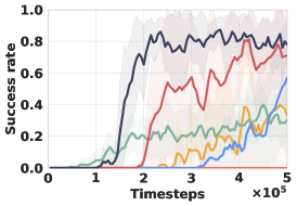
(a) Ant Maze (U-shape)

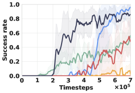
(b) Stochastic Ant Maze (U-shape)

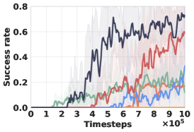
(c) Large Ant Maze (U-shape)

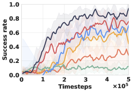
(d) Ant Maze (W-shape)

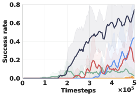
(e) Ant Maze-Bottleneck

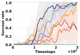
(f) Point Maze

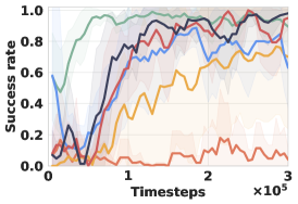
(g) Reacher

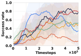
(h) Pusher

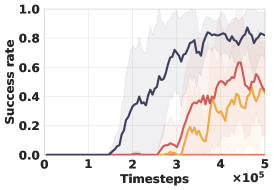
(i) Ant Maze (dense, U-shape)

Figure 2: The average success rate of multiple comparison methods on a set of environments. The solid lines represent the mean across five runs. The transparent areas represent the standard deviation. Note that in Figure 2i, the comparison on dense reward setting does not involve DHRL and PIG due to the scope and limitations of their applicability.

Comparison to existing goal-relabeling.

To justify the superiority of the proposed goal-relabeling approach over the others. We compared the proposed framework with different goal-relabeling technologies: (a) vanilla off-policy correction (OPC) in HIRO [30], (b) hindsight-based goal-relabeling in HAC [23], and (c) foresight goal inference (FGI) in MapGo [48], which is a model-based variant of vanilla hindsight-based goal-relabeling. Before making the comparison, we would like to first recognize the effectiveness of two tricks: the exponential weighting and soft-relabeling. [16] has been systematically explained that inaccuracies in learned models make long rollouts unreliable due to the compounding error. The gap between true returns and learned model returns cannot be eliminated, hence cumulative errors will be huge for too long rollouts. To address this, we employed an exponential weighting function along the horizontal axis to highlight shorter rollouts. Figure 3a illustrates the significance of the exponential weighting in suppressing cumulative errors. On the other hand, soft relabeling was utilized to enhance the robustness of goal relabeling against outliers, ensuring that the relabelled subgoals remain in close proximity to the original ones. Figure 3b provides insights into the impact of soft-relabeling on different goal-relabelling technologies. It can be observed that the soft-relabeling enhanced the robustness of different goal-relabelling technologies. In the end, we investigated the impact of the model-based gradient penalty on different goal-relabelling technologies. As shown in Figure 3c, all goal-relabelling technologies had a faster asymptotic convergence rate under gradient penalty. The result highlights the role of the gradient penalty in enhancing robustness against high-level errors, such as an unreachable or faraway goal. Figure 3c also demonstrates our proposed relabeling and HAC are comparable and outperform others.

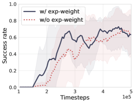
(a) Exponential Weighting

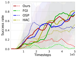
(b) Soft-Relabeling

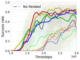
(c) Model-based Gradient Penalty

Figure 3: Figure shows the importance of components related to relabeling and compares the performance of different goal-relabeling technologies: (a) the learning curves of ACLG based on the proposed relabeling method with and without exponential weighting on Ant Maze (U-shape), (b) the learning curves of ACLG based on different goal-relabeling technologies with (solid line) and without (dotted line) the soft-relabeling on the Point Maze, and (c) the learning curves of ACLG based on different goal-relabeling technologies (after applying the soft-relabeling) with (solid line) and without (dotted line) gradient penalty on Ant Maze (U-shape).

5.2 Ablation study

In this section, we investigate the effectiveness of two crucial factors in our algorithm: the gradient penalty term and the one-step planning term. Considering that the number of lower-level critic training iterations was increased to alleviate the impact of the gradient penalty, we additionally provide a comprehensive analysis about the effects of increased iterations on various alternative methods. As depicted in Figure 4a, increasing the number of critic training iterations led to improved performance when compared to the original approach. Moreover, even without increasing the training iterations, ACLG+GCMR consistently outperformed other methods and overtook the ACLG with increased training iterations after several timesteps. The results demonstrate that the GCMR can enhance the robustness of HRL frameworks and prevent falling into local pitfalls.

Next, we highlight the importance of the hyper-parameters $\lambda_{gp}$ and $\lambda_{osrp}$. In Figure 4b, we investigate the effectiveness of $\lambda_{gp}$. Overall, the application of gradient penalty contributes to achieving better asymptotic performance compared to not using it. Furthermore, the best performance was obtained when the $\lambda_{gp}$ was set to 1.0. We validated it in multiple environments, and the value $\lambda_{gp}=1.0$ consistently emerges as optimal. In Figure 4c, we clarify the role of $\lambda_{osrp}$. One can find that a large $\lambda_{osrp}$ could powerfully and aggressively force the lower-level policy to follow the one-step rollout-based planning, leading to faster learning. However, if $\lambda_{osrp}$ is too large, the exploration capability of behavioral policy will be limited. The recommended range for the parameter $\lambda_{osrp}$ is between 0.0005 and 0.005.

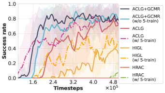
(a) The impact of increased critic iterations

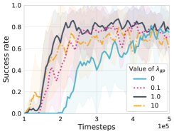
(b) Varying $\lambda_{gp}$

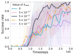
(c) Varying $\lambda_{osrp}$

Figure 4: Ablation studies on different algorithmic components. In (a), we investigate the impact of increased training iterations for critic on various HRL methods in the Ant Maze (U-shape) environment, where "5-train" indicates that the number of training iterations of lower-level critic network is increase to 5. Then, we measure the performance of ACLG+GCMR with varying number of (b) $\lambda_{gp}$ in Ant Maze (U-shape) and (c) $\lambda_{osrp}$ in Point Maze.

6 Discussion and conclusion

We present a new goal-conditioned HRL framework with Guided Cooperation via Model-based Rollout (GCMR), which uses the learned dynamics as a bridge for inter-level cooperation. Experimentally we instantiated several cooperation and communication mechanisms to improve the stability of hierarchy, achieving both data efficiency and learning efficiency. To our knowledge, very few prior works have discussed the model exploitation problem in goal-conditioned HRL. This research not only provides a SOTA HRL algorithm but also demonstrates the potential of integrating the learned dynamics model into goal-conditioned HRL, which is expected to draw the attention of researchers to such a direction.

Limitation.

This study has certain limitations. First, our experiments show that the GCMR achieved significant performance improvement, and such improvement came at the expense of more computational cost (see Table 4 in Appendix F.3 for a quantitative analysis of computational cost). However, the time-consuming issue only occurs during the training stage and will not affect the execution response time in the applications. Second, we need to clarify that the scope of applicability is off-policy goal-conditioned HRL. The effectiveness in general RL tasks or online tasks had not been validated. Third, the experimental environments used in this study have 7 or 30 dimensions. Moreover, our network architecture of transition dynamics models is relatively simple, leading to limited regression capability. Applications in environments that closely resemble real-world scenarios with high-dimensional state observation, like the large-scale point cloud environments encountered in autonomous driving, might face limitations. This issue will be investigated in our future work.

Appendix A Algorithms

We provide the GCMR algorithm below.

Algorithm 1 Guided Cooperation via Model-based Rollout (GCMR)

Input:

• Key hyper-parameters: the number of candidate goals $k$, gradient penalty loss coefficient $\lambda_{gp}$, one-step planning term coefficient$\lambda_{osrp}$, soft update rate of the shift magnitude within relabeling $\epsilon$.

• General hyper-parameters: the subgoal scheme $\eta$ (set to 0/1 for the relative/absolute scheme), training batch number $BN$, higher-level update frequency $H_{c}$, learning frequency of dynamics models $D_{c}$, initial steps without using dynamics models $t_{dm}$, usage frequencies of gradient penalty and planning term $GP_{c}$, $OP_{c}$.

Initialize all actor and critic networks with random parameters $\theta_{lo}$, $\theta_{hi}$, $\phi_{lo}$, $\phi_{hi}$.

Initialize the dynamics models $\Gamma_{\xi}$.

$\mathcal{D}_{lo}\leftarrow\emptyset$, $\mathcal{D}_{hi}\leftarrow\emptyset$ $\triangleright$ Initialize replay buffers

while True do

     $t\leftarrow 0$

     Reset the environment and get the state $s_{t}$ and episode terminal signal $done$.

     repeat

         if $t\equiv 0$ (mod $c$) then

              Generate subgoal $sg_{t}\sim\pi\left(sg|s_{t},g;\theta_{hi}\right)$.

         else

              Obtain goal through the transition function $sg_{t}=sg_{t-1}+(\neg\eta)\cdot\varphi(s_{t-1}-s_{t})$.

         end if

         $a_{t}\sim\pi\left(a|s_{t},sg_{t};\theta_{lo}\right)$ $\triangleright$ Sample lower-level action

         $s_{t+1}$, $r_{t}$ $\leftarrow{\rm env.step}(a_{t})$ $\triangleright$ Perform action $a_{t}$ in the environment

         $\mathcal{D}_{lo}\leftarrow\mathcal{D}_{lo}\cup\{\tau_{lo}\}$, $\mathcal{D}_{hi}\leftarrow\mathcal{D}_{hi}\cup\{\tau_{hi}\}$ $\triangleright$ Store transitions into buffers

         $t\leftarrow t+1$

     until $done$ is $true$.

     if $t>t_{dm}$ then

         if $t\equiv 0$ (mod $D_{c}$) then

              Train the dynamics models $\Gamma_{\xi}$.

         end if

         Randomly sample experiences from replay buffers.

         Relabel subgoals via the rollout-based off-policy correction.

         if $t\equiv 0$ (mod $GP_{c}$) then repeat 5 times

              $\mathcal{L}(\phi_{lo})\leftarrow\mathcal{L}_{gp}(\phi_{lo})+\mathcal{L}(\phi_{lo})$ $\triangleright$ Plug the gradient penalty into critic loss end repeat

         end if

         if $t\equiv 0$ (mod $OP_{c}\times H_{c}$) then

              $\mathcal{L}(\theta_{lo})\leftarrow\mathcal{L}_{osrp}+\mathcal{L}(\theta_{lo})$ $\triangleright$ Plug the planning term into actor loss

         end if

     end if

end while

Appendix B Disentangled Variant of HIGL [17]: ACLG

Adjacency Constraint.

For the high-level subgoal generation, reachability within $c$ steps is a sufficient condition for facilitating reasonable exploration. Zhang et al. [46, 47] mined the adjacency information from gathered trajectories by the changing behavioral policy over time during the training procedure. In that study, a $c$-step adjacency matrix was constructed to memorize $c$-step adjacent state-pairs appearing in the agent’s trajectories. To ensure this procedure is differentiable and can be generalized to newly-visited states, the adjacency information stored in such matrix was further distilled into an adjacency network $\psi$ parameterized by $\Phi$. Specifically, the adjacency network approximates a mapping from a goal space into an adjacency space. Subsequently, the resulted embeddings can be utilized to measure whether two states are $c$-step adjacent using the Euclidean distance. For example, the $c$-step adjacent estimation (or shortest transition distance) of two states $s_{i}$ and $s_{j}$ can be calculated as: $d_{st}(s_{i},s_{j};\Phi)\approx\frac{c}{\zeta_{c}}||\psi_{\Phi}(\varphi(s_{i}))-\psi_{\Phi}(\varphi(s_{j}))||_{2}$, where $\zeta_{c}$ is a scaling factor and the $\varphi$ function maps states into the goal space. Such an adjacency network can be learned by minimizing the following contrastive-like loss: $\mathcal{L}_{{\rm adj}}(\Phi)=\mathbb{E}_{s_{i},s_{j}\in\mathcal{S}}[l\cdot\max(||\psi_{\Phi}(\varphi(s_{i}))-\psi_{\Phi}(\varphi(s_{j}))||_{2}-\zeta_{c},0)+(1-l)\cdot\max(\zeta_{c}+\delta_{\rm adj}-||\psi_{\Phi}(\varphi(s_{i}))-\psi_{\Phi}(\varphi(s_{j}))||_{2},0)]$, where $\delta_{\rm adj}>0$ is a hyper-parameter indicating a margin between embeddings and $l\in\{0,1\}$ is the label indicating whether $s_{i}$ and $s_{j}$ are adjacent in the $k$-step.

Landmark-based Planning.

Graph-based navigation has become a popular technique for solving complex and sparse reward tasks by providing a long-term horizon. The relevant frameworks [35, 15, 8, 7, 42, 17, 45, 21, 18] commonly contain two components: (a) a graph built by sampling landmarks and (b) a graph planner to select waypoints. In a graph, each node corresponds to an observation state while edges between nodes are weighted using a distance estimation. Specifically, a set of observations randomly subsampling from the replay buffer are organized as nodes, where high-dimensional samples (e.g., images) may be embedded into low-dimensional representations [35, 8, 26, 42, 45]. However, operations over the direct subsampling of the replay buffer will be costly. The state aggregation [7] and landmark sampling based on farthest point sampling (FPS) were proposed for further sparsification [15, 17, 21, 18]. Our study follows prior works of Kim et al. [17, 18], in which FPS was employed to select a collection of landmarks, i.e., coverage-based landmarks ${LM}^{\rm cov}$, from the replay buffer. In addition to this, HIGL [17] used random network distillation [3] to explicitly sample novel landmarks, i.e., novelty-based landmarks ${LM}^{\rm nov}$, a set of states rarely visited in the past. Hence, the final collection of landmarks was ${LM}={LM}^{\rm cov}\cup{LM}^{\rm nov}$. Once landmarks are added to the graph, the edge weight between any two vertices can be estimated by a lower-level value function [15, 8, 17, 21, 18] or the (Euclidean-based or contrastive-loss-based) distance between low-dimensional embeddings of states [35, 42, 26, 46]. Following prior works [15, 17, 18], in this study, we estimated the edge weight via the lower-level value function, i.e., $-V_{lo}(s_{i},\varphi(s_{j}))\approx-Q(s_{i},\varphi(s_{j}),\pi\left(a|s_{i},\varphi(s_{j});\theta_{lo}\right);\phi_{lo}),\forall s_{i},s_{j}\in LM$. After that, unreachable edges were clipped by a preset threshold [15]. In the end, the shortest path planning algorithm was run to plan the next subgoal which is the very first landmark in the shortest path from the current state $s_{t}$ to the goal $g$:

$$sg_{t}^{\rm plan}=\arg\min_{\varphi(s_{i})}-[V_{lo}(s_{t},\varphi(s_{i}))+V_{lo}(s_{i},g)],\quad\forall s_{i}\in{LM}^{\rm cov}\cup{LM}^{\rm nov}.$$ (18)

Adjacency Constraint and Landmark-based Planning: ACLG.

In HIGL, after finding a landmark through landmark-based planning (see Equation 18), the raw selected landmark was shifted towards the current state $s_{t}$ for reachability: $sg_{t}^{\rm pseudo}=sg_{t}^{\rm plan}+\delta_{\rm pseudo}\cdot\frac{sg_{t}^{\rm plan}-\varphi(s_{t})}{||sg_{t}^{\rm plan}-\varphi(s_{t})||_{2}}$, where $\delta_{\rm pseudo}$ denotes the shift magnitude. Then the higher-level policy was guided to generate subgoals adjacent to the planned landmarks and the landmark loss of HIGL was formulated as:

$$\mathcal{L}^{\rm HIGL}_{\rm landmark}(\theta_{hi})=\lambda^{\rm HIGL}_{\rm landmark}\cdot\max(||\psi_{\Phi}(sg_{t}^{\rm pseudo})-\psi_{\Phi}(\pi(s_{t},g;\theta_{hi}))||-\zeta_{c},0)$$ (19)

Here, Kim et al. employed the adjacency constraint to encourage the generated subgoals to be in the $c$-step adjacent region to the planned landmark. However, the performance of HIGL is limited due to the entanglement between the adjacency constraint and landmark-based planning. Inspired by PIG [18], we proposed a disentangled variant of HIGL. We only made minor modifications to the landmark loss of HIGL, which was re-formulated as:

$$\mathcal{L}^{\rm ACLG}(\theta_{hi})= \lambda_{\rm adj}\cdot\max(||\psi_{\Phi}(\varphi(s_{t}))-\psi_{\Phi}(\pi(s_{t},g;\theta_{hi}))||-\zeta_{c},0)$$ (20)

$$+\lambda^{\rm ACLG}_{\rm landmark}\cdot||sg_{t}^{\rm pseudo}-\pi(s_{t},g;\theta_{hi})||^{2}_{2}$$

The former term is the Adjacency Constraint and the latter is the Landmark-Guided loss, so it was called ACLG. The hyperparameters $\lambda_{\rm adj}$ and $\lambda^{\rm ACLG}_{\rm landmark}$ were introduced to better balance the adjacency constraint and landmark-based planning.

Appendix C Lipschitz Property of the Q-function w.r.t. action

In this appendix, we provide a brief proof for Proposition 1. More detailed proof can be found in [13]. We start out with a lemma that helps with subsequent derivation.

Lemma 1.

Assume policy gradients w.r.t. input actions in an MDP admit a bound at any time $t$: $\|\frac{\partial\pi^{*}(a_{t+1}|s_{t+1})}{\partial a_{t}}\|_{F}\leq L_{\pi}$. Then the following holds for any non-negative integer $c$ and $t$:

$$\big{|}\nabla_{a_{t}}\mathbb{E}_{s_{t+c}|s_{t}}[r^{*}(s_{t+c},a_{t+c})]\big{|}\leq L_{\pi}\mathbb{E}_{s_{t+c}|s_{t}}\big{|}\nabla_{a_{t+1}}\mathbb{E}_{s_{t+c}|s_{t+1}}[r^{*}(s_{t+c},a_{t+c})]\big{|}$$ (21)

Proof.

$$\begin{split}\big{|}\nabla_{a_{t}}\mathbb{E}_{s_{t+c}|s_{t}}[r^{*}(s_{t+c},a_{t+c})]&=\big{|}\nabla_{a_{t}}\mathbb{E}_{s_{t+1}|s_{t}}\mathbb{E}_{s_{t+c}|s_{t+1}}[r^{*}(s_{t+c},a_{t+c})]\cdot\frac{\partial a_{t+1}}{\partial a_{t}}\big{|}\\ &\leq\big{|}\nabla_{a_{t}}\mathbb{E}_{s_{t+1}|s_{t}}\mathbb{E}_{s_{t+c}|s_{t+1}}[r^{*}(s_{t+c},a_{t+c})]\big{|}\cdot\big{|}\frac{\partial a_{t+1}}{\partial a_{t}}\big{|}\\ &\leq\big{|}\nabla_{a_{t}}\mathbb{E}_{s_{t+1}|s_{t}}\mathbb{E}_{s_{t+c}|s_{t+1}}[r^{*}(s_{t+c},a_{t+c})]\big{|}\cdot L_{\pi}\\ &=\mathbb{E}_{s_{t+1}|s_{t}}\big{|}\nabla_{a_{t}}\mathbb{E}_{s_{t+c}|s_{t+1}}[r^{*}(s_{t+c},a_{t+c})]\big{|}\cdot L_{\pi}\end{split}$$ (22)

∎

Remark 2.

Lemma 21 gives the discrepancy of reward gradients starting from adjacent states. We can apply this lemma sequentially and infer the upper bound of reward gradients:

$$\begin{split}\big{|}\nabla_{a_{t}}\mathbb{E}_{s_{t+c}|s_{t}}&[r^{*}(s_{t+c},a_{t+c})]\big{|}=\big{|}\nabla_{a_{t}}\mathbb{E}_{s_{t+1}|s_{t}}\mathbb{E}_{s_{t+c}|s_{t+1}}[r^{*}(s_{t+c},a_{t+c})]\cdot\frac{\partial a_{t+1}}{\partial a_{t}}\big{|}\\ &\leq\mathbb{E}_{s_{t+1}|s_{t}}\big{|}\nabla_{a_{t}}\mathbb{E}_{s_{t+c}|s_{t+1}}[r^{*}(s_{t+c},a_{t+c})]\big{|}\cdot L_{\pi}\\ &\leq\mathbb{E}_{s_{t+1}|s_{t}}\mathbb{E}_{s_{t+2}|s_{t+1}}\dots\mathbb{E}_{s_{t+c}|s_{t+c-1}}\big{|}\nabla_{a_{t}}\mathbb{E}_{s_{t+c}|s_{t+c}}[r^{*}(s_{t+c},a_{t+c})]\big{|}\cdot(L_{\pi})^{c}\\ &=\mathbb{E}_{s_{t+c}|s_{t}}\big{|}\nabla_{a_{t}}r^{*}(s_{t+c},a_{t+c})\big{|}\cdot(L_{\pi})^{c}\end{split}$$ (23)

Proposition 2.

Let $\pi^{*}(a_{t}|s_{t})$ and $r^{*}(s_{t},a_{t})$ be the policy and the reward function in an MDP. Suppose there are the upper bounds of Frobenius norm of the policy and reward gradients w.r.t. input actions, i.e., $\|\frac{\partial\pi^{*}(a_{t+1}|s_{t+1})}{\partial a_{t}}\|_{F}\leq L_{\pi}<1$ and $\|\frac{\partial r^{*}(s_{t+1},a_{t+1})}{\partial a_{t}}\|_{F}\leq L_{r}$. Then the gradient of the learned Q-function w.r.t. action can be upper-bounded as:

$$\|\nabla_{a_{t}}Q_{\pi^{*}}(s_{t},a_{t})\|_{F}\leq\frac{\sqrt{N}L_{r}}{1-\gamma L_{\pi}}$$ (24)

Where $N$ denotes the dimension of the action and $\gamma$ is the discount factor.

Proof.

$$\begin{split}\|\nabla_{a_{t}}Q_{\pi^{*}}(s_{t},a_{t})\|^{2}_{F}&=\sum_{i=0}^{N}\left(\nabla_{a^{i}_{t}}Q_{\pi^{*}}(s_{t},a_{t})\right)^{2}\\ &=\sum_{i=0}^{N}\left(\sum_{c=0}^{\infty}\gamma^{c}\nabla_{a^{i}_{t}}\mathbb{E}_{s_{t+c}|s_{t}}[r^{*}(s_{t+c},a_{t+c})]\right)^{2}\\ &\leq\sum_{i=0}^{N}\left(\sum_{c=0}^{\infty}\gamma^{c}\big{|}\nabla_{a^{i}_{t}}\mathbb{E}_{s_{t+c}|s_{t}}[r^{*}(s_{t+c},a_{t+c})]\big{|}\right)^{2}\end{split}$$ (25)

Meanwhile according to Remark 23, we have:

$$\begin{split}\big{|}\nabla_{a_{t}}\mathbb{E}_{s_{t+c}|s_{t}}[r^{*}(s_{t+c},a_{t+c})]\big{|}&\leq\mathbb{E}_{s_{t+c}|s_{t}}\big{|}\nabla_{a^{i}_{t}}r^{*}(s_{t+c},a_{t+c})\big{|}\cdot(L_{\pi})^{c}\\ &\leq\mathbb{E}_{s_{t+c}|s_{t}}L_{r}\cdot(L_{\pi})^{c}\\ &=L_{r}\cdot(L_{\pi})^{c}\end{split}$$ (26)

Replacing the above gradient term, then the formula 25 can be rewritten as:

$$\begin{split}\|\nabla_{a_{t}}Q_{\pi^{*}}(s_{t},a_{t})\|^{2}_{F}&\leq\sum_{i=0}^{N}\left(\sum_{c=0}^{\infty}\gamma^{c}\big{|}\nabla_{a_{t}}\mathbb{E}_{s_{t+c}|s_{t}}[r^{*}(s_{t+c},a_{t+c})]\big{|}\right)^{2}\\ &\leq\sum_{i=0}^{N}\left(\sum_{c=0}^{\infty}\gamma^{c}\cdot L_{r}\cdot L_{\pi}^{c}\right)^{2}=N\left(L_{r}\sum_{c=0}^{\infty}(\gamma\cdot L_{\pi})^{c}\right)^{2}\\ &=N\left(\frac{L_{r}}{1-\gamma L_{\pi}}\right)^{2}\end{split}$$ (27)

The above inequality on the sqrt function then implies:

$$\begin{split}\|\nabla_{a_{t}}Q_{\pi^{*}}(s_{t},a_{t})\|_{F}\leq\frac{\sqrt{N}L_{r}}{1-\gamma L_{\pi}}\end{split}$$ (28)

Which completes the proof. ∎

Appendix D Environment Details

Most experiments were conducted under the same environments as that in [17], including Point Maze, Ant Maze (W-shape), Ant Maze (U-shape), Pusher, and Reacher. Further detail is available in public repositories 1 . Besides, we introduced a more challenging locomotion environment, i.e., Ant Maze-Bottleneck, to validate the stability and robustness of the proposed GCMR in long-horizon and complicated tasks requiring delicate controls.

Ant Maze-Bottleneck

The Ant Maze-Bottleneck environment was first introduced in [21], which provided implementation details in public repositories in 1 . In this study, we resized it to be the same as the other mazes. Specifically, the size of the environment is $12\times 12$. At training time, a goal point was selected randomly from a two-dimensional planar where both $x$- and $y$-axes range from -2 to 10. At evaluation time, the goal was placed at (0, 8) (i.e., the top left corner). A minimum threshold of competence was set to an L2 distance of 2.5 from the goal. Each episode would be terminated after 600 steps.

Appendix E Experimental Configurations

E.1 Network Structure

For a fair comparison, we adopted the same architecture as [46, 17]. In detail, all actor and critic networks had two hidden layers composed of a fully connected layer with 300 units and a ReLU nonlinearity function. The output layer in actor networks had the same number of cells as the dimension of the action space and normalized the output to $[-1,1]$ using the $tanh$ function. After that, the output was rescaled to the range of action space.

For the dynamics model, the ensemble size $B$ was set to 5, a recommended value in [5]. Each of the ensembles was instantiated with three layers, similar to the above actor network. Yet, each hidden layer had 256 units and was followed by the Swish activation [34]. Note that units of the output layer were twice as much as the actor because the action distribution was represented with the mean and covariance of a Gaussian.

The Adam optimizer was utilized for all networks.

E.2 Hyper-Parameter Settings

We list hyper-parameters used across all environments in Table 1. Hyper-parameters that differ across the environments are presented in Table 2. These hyper-parameters involving HIGL remained the same as proposed by [17]. Besides, the update speed of the shift magnitude of goals was set at 0.01.

Table 1: Hyper-parameters across all environments.

Hyper-parameters	Value
	Higher-level	Lower-level
Actor learning rate	0.0001	0.0001
Critic learning rate	0.001	0.001
Soft update rate	0.005	0.005
$\gamma$	0.99	0.95
Reward scaling	0.1	1.0
Training frequency $H_{c}$	10	1
Batch size	128	128
Candidates’ number	10
$\lambda^{\rm ACLG}_{\rm landmark}$	1.0
$\lambda_{gp}$		1.0
$\lambda_{osrp}$		0.005 $\sim$ 0.0005*
$\lambda_{gp}$ usage frequencies $GP_{c}$		5
$\lambda_{osrp}$ usage frequencies $OP_{c}$		10
	Dynamics model
Ensemble number	5
Learning rate	0.005
Batch size	256
Training epochs	20 $\sim$ 50

• Only $\lambda_{osrp}=0.005$ for the Point Maze, while $\lambda_{osrp}$ are set to 0.0005 for others.

Table 2: Hyper-parameters that differ across the environments.

Hyper-parameters	Maze-baseda	Arm-basedb
	Higher-level
High-level action frequency	10	5
Exploration strategy	Gaussian ($\sigma=1.0$)	Gaussian ($\sigma=0.2$)
	Lower-level
Exploration strategy	Gaussian ($\sigma=1.0$)	Gaussian ($\sigma=0.1$)
$\lambda_{\rm adj}$	20.0	0
	Dynamics model
Training frequency $D_{c}$	2000	500
Initial steps w/o model $t_{dm}$	20000	10000

• Maze-based environments include Point Maze, Ant Maze (U/W-shape), and Ant Maze-Bottleneck.

• Arm-based environments are Pusher and Reacher.

Table 3: Number of Landmarks

Environments	GCMR$+$ACLG*	ACLG*	HIGL*	DHRL	PIG
Ant Maze (U-shape)	60$+$60		20$+$20	300	400
Ant Maze (W-shape)	60$+$60		60$+$60	300	400
Point Maze	60$+$60		20$+$20	300	200
Arm-based	20$+$20		20$+$20	300	80

• Where $+$ connects the numbers of coverage-based landmarks and novelty-based landmarks.

Appendix F Additional Experiments

F.1 Hyperparameters in ACLG

Additionally, we conduct experiments on Ant Maze (U-shape) to verify the effectiveness of hyperparameters, (1) the number of landmarks and (2) the balancing coefficient $\lambda^{\rm ACLG}_{\rm landmark}$.

Landmark Number Selection.

Since the number of landmarks plays an important role in the graph-related method, we explored the effects of different numbers of landmarks on performance. Here, we sample the same number of landmarks for each criterion, i.e., the same number for novelty-based and novelty-based landmarks ${LM}^{\rm nov}={LM}^{\rm nov}$. As shown in Figure 5a, overall, with the same number of landmarks, the ACLG significantly outperforms the HIGL since the disentanglement between the adjacency constraint and landmark-based planning further highlights the advantages of landmarks.

Balancing Coefficient $\lambda^{\rm ACLG}_{\rm landmark}$.

In Figure 5b, we investigate the effectiveness of the balancing coefficient $\lambda^{\rm ACLG}_{\rm landmark}$, which determines the effect of the landmark-based planning term in ACLG on performance. We find that ACLG with $\lambda^{\rm ACLG}_{\rm landmark}=1.0$ outperforms others. We find that PIG with $\lambda^{\rm ACLG}_{\rm landmark}\in\{1.0,10\}$ outperforms PIG with $\lambda^{\rm ACLG}_{\rm landmark}=0.1$, which shows a large value of $\lambda^{\rm ACLG}_{\rm landmark}$ helps unleash the guiding role of landmarks.

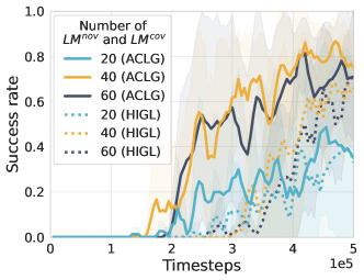
(a) Number of landmarks

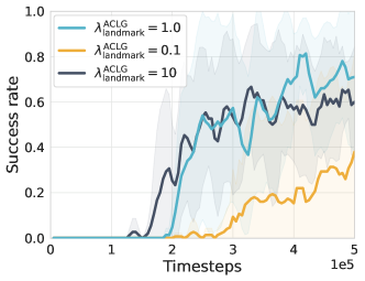
(b) Varying $\lambda^{\rm ACLG}_{\rm landmark}$

Figure 5: Ablation studies on landmark-related components. We measure the performance of ACLG by (a) varying number of landmarks and (b) varying balancing coefficient $\lambda^{\rm ACLG}_{\rm landmark}$ in Ant Maze (U-shape).

F.2 GCMR Solely Employed for Goal-Reaching Tasks

In our experiments, the proposed GCMR was used as an additional plugin. Of course, GCMR can be solely applicable to goal-reaching tasks. We conducted experiments in the Point Maze and Ant Maze (U-shape) tasks. As shown in Figure 6, the results indicate that GCMR can be used independently and achieve similar results to HIGL. Meanwhile, in Figure 7, we investigate how the gradient penalty term and the one-step planning term impact the final performance when solely using the GCMR method in Ant Maze (U-shape). Figure 7 illustrates similar conclusions as those in the previous Figure 4.

(a)

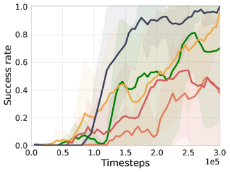
(a) Point Maze

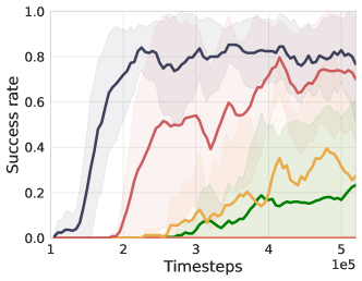
(b) Ant Maze (U-shape)

Figure 6: Performance when solely using the GCMR method in environments (a) Point Maze and (b) Ant Maze (U-shape). The solid lines represent the mean across five runs. The transparent areas represent the standard deviation.

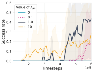
(a) Varying $\lambda_{gp}$

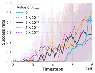
(b) Varying $\lambda_{osrp}$

Figure 7: Impact of varying (a) $\lambda_{gp}$ and (b) $\lambda_{osrp}$ in the Ant Maze (U-shape) environment, when solely using the GCMR method.

F.3 Quantification of Extra Computational Cost

The extra computational cost is primarily composed of three aspects:

• (1) dynamic model training,

• (2) model-based gradient penalty and one-step rollout planning in low-level policy training,

• (3) goal-relabeling in high-level policy training.

Therefore, we ran both methods ACLG+GCMR and ACLG on Ant Maze (U-shape) for $0.7\times 10^{5}$ steps to compare their runtime in these aspects.

Table 4: Quantification of Extra Computational Cost

Training time (s)	Total	Dynamic model	Low-level policy	High-level policy
ACLG+GCMR	5065.18	16.51	3603.01	854.64
ACLG	1845.63	0	632.97	614.01

References

- Andrychowicz et al. [2017] Marcin Andrychowicz, Filip Wolski, Alex Ray, Jonas Schneider, Rachel Fong, Peter Welinder, Bob McGrew, Josh Tobin, Abbeel Pieter, and Wojciech Zaremba. Hindsight experience replay. Advances in neural information processing systems, 30, 2017.
- Buckman et al. [2018] Jacob Buckman, Danijar Hafner, George Tucker, Eugene Brevdo, and Honglak Lee. Sample-efficient reinforcement learning with stochastic ensemble value expansion. Advances in neural information processing systems, 31, 2018.
- Burda et al. [2018] Yuri Burda, Harrison Edwards, Amos Storkey, and Oleg Klimov. Exploration by random network distillation. In International Conference on Learning Representations, 2018.
- Byravan et al. [2020] Arunkumar Byravan, Jost Tobias Springenberg, Abbas Abdolmaleki, Roland Hafner, Michael Neunert, Thomas Lampe, Noah Siegel, Nicolas Heess, and Martin Riedmiller. Imagined value gradients: Model-based policy optimization with tranferable latent dynamics models. In Conference on Robot Learning, pages 566–589. PMLR, 2020.
- Chua et al. [2018] Kurtland Chua, Roberto Calandra, Rowan McAllister, and Sergey Levine. Deep reinforcement learning in a handful of trials using probabilistic dynamics models. Advances in neural information processing systems, 31, 2018.
- Dayan and Hinton [1992] Peter Dayan and Geoffrey E Hinton. Feudal reinforcement learning. Advances in neural information processing systems, 5, 1992.
- Emmons et al. [2020] Scott Emmons, Ajay Jain, Misha Laskin, Thanard Kurutach, Pieter Abbeel, and Deepak Pathak. Sparse graphical memory for robust planning. Advances in Neural Information Processing Systems, 33:5251–5262, 2020.
- Eysenbach et al. [2019] Ben Eysenbach, Russ R Salakhutdinov, and Sergey Levine. Search on the replay buffer: Bridging planning and reinforcement learning. Advances in Neural Information Processing Systems, 32, 2019.
- Fedus et al. [2020] William Fedus, Prajit Ramachandran, Rishabh Agarwal, Yoshua Bengio, Hugo Larochelle, Mark Rowland, and Will Dabney. Revisiting fundamentals of experience replay. In International Conference on Machine Learning, pages 3061–3071. PMLR, 2020.
- Feinberg et al. [2018] Vladimir Feinberg, Alvin Wan, Ion Stoica, Michael I Jordan, Joseph E Gonzalez, and Sergey Levine. Model-based value expansion for efficient model-free reinforcement learning. In International Conference on Machine Learning, 2018.
- Florensa et al. [2017] Carlos Florensa, Yan Duan, and Pieter Abbeel. Stochastic neural networks for hierarchical reinforcement learning. In International Conference on Learning Representations, 2017.
- Fujimoto et al. [2018] Scott Fujimoto, Herke Hoof, and David Meger. Addressing function approximation error in actor-critic methods. In International conference on machine learning, pages 1587–1596. PMLR, 2018.
- Gao et al. [2022] Chengqian Gao, Ke Xu, Liu Liu, Deheng Ye, Peilin Zhao, and Zhiqiang Xu. Robust offline reinforcement learning with gradient penalty and constraint relaxation. CoRR, abs/2210.10469, 2022. doi: 10.48550/arXiv.2210.10469. URL https://doi.org/10.48550/arXiv.2210.10469.
- Gulrajani et al. [2017] Ishaan Gulrajani, Faruk Ahmed, Martin Arjovsky, Vincent Dumoulin, and Aaron C Courville. Improved training of wasserstein gans. Advances in neural information processing systems, 30, 2017.
- Huang et al. [2019] Zhiao Huang, Fangchen Liu, and Hao Su. Mapping state space using landmarks for universal goal reaching. Advances in Neural Information Processing Systems, 32, 2019.
- Janner et al. [2019] Michael Janner, Justin Fu, Marvin Zhang, and Sergey Levine. When to trust your model: Model-based policy optimization. Advances in neural information processing systems, 32, 2019.
- Kim et al. [2021] Junsu Kim, Younggyo Seo, and Jinwoo Shin. Landmark-guided subgoal generation in hierarchical reinforcement learning. Advances in Neural Information Processing Systems, 34:28336–28349, 2021.
- Kim et al. [2022] Junsu Kim, Younggyo Seo, Sungsoo Ahn, Kyunghwan Son, and Jinwoo Shin. Imitating graph-based planning with goal-conditioned policies. In The Eleventh International Conference on Learning Representations, 2022.
- Kumar et al. [2019] Aviral Kumar, Justin Fu, Matthew Soh, George Tucker, and Sergey Levine. Stabilizing off-policy q-learning via bootstrapping error reduction. Advances in Neural Information Processing Systems, 32, 2019.
- Kurutach et al. [2018] Thanard Kurutach, Ignasi Clavera, Yan Duan, Aviv Tamar, and Pieter Abbeel. Model-ensemble trust-region policy optimization. In International Conference on Learning Representations, 2018.
- Lee et al. [2022] Seungjae Lee, Jigang Kim, Inkyu Jang, and H Jin Kim. Dhrl: A graph-based approach for long-horizon and sparse hierarchical reinforcement learning. In Advances in Neural Information Processing Systems, 2022.
- Levine and Koltun [2013] Sergey Levine and Vladlen Koltun. Guided policy search. In International conference on machine learning, pages 1–9. PMLR, 2013.
- Levy et al. [2019] Andrew Levy, George Konidaris, Robert Platt, and Kate Saenko. Learning multi-level hierarchies with hindsight. In Proceedings of International Conference on Learning Representations, 2019.
- Li et al. [2021] Siyuan Li, Lulu Zheng, Jianhao Wang, and Chongjie Zhang. Learning subgoal representations with slow dynamics. In International Conference on Learning Representations, 2021.
- Lillicrap et al. [2016] Timothy P. Lillicrap, Jonathan J. Hunt, Alexander Pritzel, Nicolas Heess, Tom Erez, Yuval Tassa, David Silver, and Daan Wierstra. Continuous control with deep reinforcement learning. In International Conference on Learning Representations, 2016.
- Liu et al. [2020] Kara Liu, Thanard Kurutach, Christine Tung, Pieter Abbeel, and Aviv Tamar. Hallucinative topological memory for zero-shot visual planning. In International Conference on Machine Learning, pages 6259–6270. PMLR, 2020.
- Luo et al. [2023] Fan-Ming Luo, Tian Xu, Hang Lai, Xiong-Hui Chen, Weinan Zhang, and Yang Yu. A survey on model-based reinforcement learning. SCIENCE CHINA Information Sciences, 2023.
- Luo et al. [2019] Yuping Luo, Huazhe Xu, Yuanzhi Li, Yuandong Tian, Trevor Darrell, and Tengyu Ma. Algorithmic framework for model-based deep reinforcement learning with theoretical guarantees. In International Conference on Learning Representations, 2019.
- Moerland et al. [2023] Thomas M Moerland, Joost Broekens, Aske Plaat, Catholijn M Jonker, et al. Model-based reinforcement learning: A survey. Foundations and Trends® in Machine Learning, 16(1):1–118, 2023.
- Nachum et al. [2018] Ofir Nachum, Shixiang Shane Gu, Honglak Lee, and Sergey Levine. Data-efficient hierarchical reinforcement learning. Advances in neural information processing systems, 31, 2018.
- Nachum et al. [2019] Ofir Nachum, Shixiang Gu, Honglak Lee, and Sergey Levine. Near-optimal representation learning for hierarchical reinforcement learning. In International Conference on Learning Representations, 2019.
- Nair and Finn [2020] Suraj Nair and Chelsea Finn. Hierarchical foresight: Self-supervised learning of long-horizon tasks via visual subgoal generation. In International Conference on Learning Representations, 2020.
- Pong et al. [2018] Vitchyr Pong, Shixiang Gu, Murtaza Dalal, and Sergey Levine. Temporal difference models: Model-free deep rl for model-based control. In International Conference on Learning Representations, 2018.
- Ramachandran et al. [2018] Prajit Ramachandran, Barret Zoph, and Quoc V. Le. Searching for activation functions. In International Conference on Learning Representations, 2018. URL https://openreview.net/forum?id=SkBYYyZRZ.
- Savinov et al. [2018] Nikolay Savinov, Alexey Dosovitskiy, and Vladlen Koltun. Semi-parametric topological memory for navigation. In International Conference on Learning Representations, 2018.
- Shen et al. [2020] Jian Shen, Han Zhao, Weinan Zhang, and Yong Yu. Model-based policy optimization with unsupervised model adaptation. Advances in Neural Information Processing Systems, 33:2823–2834, 2020.
- Silver et al. [2014] David Silver, Guy Lever, Nicolas Heess, Thomas Degris, Daan Wierstra, and Martin Riedmiller. Deterministic policy gradient algorithms. In International conference on machine learning, pages 387–395. Pmlr, 2014.
- Simsek et al. [2005] Ozgür Simsek, Alicia P Wolfe, and Andrew G Barto. Identifying useful subgoals in reinforcement learning by local graph partitioning. In International conference on Machine learning, pages 816–823, 2005.
- Sutton [1991] Richard S Sutton. Dyna, an integrated architecture for learning, planning, and reacting. ACM Sigart Bulletin, 2(4):160–163, 1991.
- Vezhnevets et al. [2017] Alexander Sasha Vezhnevets, Simon Osindero, Tom Schaul, Nicolas Heess, Max Jaderberg, David Silver, and Koray Kavukcuoglu. Feudal networks for hierarchical reinforcement learning. In International Conference on Machine Learning, pages 3540–3549. PMLR, 2017.
- Wang et al. [2023] Vivienne Huiling Wang, Joni Pajarinen, Tinghuai Wang, and Joni-Kristian Küamüarüainen. State-conditioned adversarial subgoal generation. In Proceedings of the AAAI Conference on Artificial Intelligence, 2023.
- Yang et al. [2020] Ge Yang, Amy Zhang, Ari Morcos, Joelle Pineau, Pieter Abbeel, and Roberto Calandra. Plan2vec: Unsupervised representation learning by latent plans. In Learning for Dynamics and Control, pages 935–946. PMLR, 2020.
- Yu et al. [2020] Tianhe Yu, Garrett Thomas, Lantao Yu, Stefano Ermon, James Y Zou, Sergey Levine, Chelsea Finn, and Tengyu Ma. Mopo: Model-based offline policy optimization. Advances in Neural Information Processing Systems, 33:14129–14142, 2020.
- Yu et al. [2021] Tianhe Yu, Aviral Kumar, Rafael Rafailov, Aravind Rajeswaran, Sergey Levine, and Chelsea Finn. Combo: Conservative offline model-based policy optimization. Advances in neural information processing systems, 34:28954–28967, 2021.
- Zhang et al. [2021] Lunjun Zhang, Ge Yang, and Bradly C Stadie. World model as a graph: Learning latent landmarks for planning. In International Conference on Machine Learning, pages 12611–12620. PMLR, 2021.
- Zhang et al. [2020] Tianren Zhang, Shangqi Guo, Tian Tan, Xiaolin Hu, and Feng Chen. Generating adjacency-constrained subgoals in hierarchical reinforcement learning. Advances in Neural Information Processing Systems, 33:21579–21590, 2020.
- Zhang et al. [2022] Tianren Zhang, Shangqi Guo, Tian Tan, Xiaolin Hu, and Feng Chen. Adjacency constraint for efficient hierarchical reinforcement learning. IEEE Transactions on Pattern Analysis and Machine Intelligence, 45(4):4152–4166, 2022.
- Zhu et al. [2021] Menghui Zhu, Minghuan Liu, Jian Shen, Zhicheng Zhang, Sheng Chen, Weinan Zhang, Deheng Ye, Yong Yu, Qiang Fu, and Wei Yang. Mapgo: Model-assisted policy optimization for goal-oriented tasks. International Joint Conference on Artificial Intelligence, 2021.