Controller Synthesis of Collaborative Signal Temporal Logic Tasks for Multi-Agent Systems via Assume-Guarantee Contracts

Abstract

This paper considers the problem of controller synthesis of signal temporal logic (STL) specifications for large-scale multi-agent systems, where the agents are dynamically coupled and subject to collaborative tasks. A compositional framework based on continuous-time assume-guarantee contracts is developed to break the complex and large synthesis problem into subproblems of manageable sizes. We first show how to formulate the collaborative STL tasks as assume-guarantee contracts by leveraging the idea of funnel-based control. The concept of contracts is used to establish our compositionality result, which allows us to guarantee the satisfaction of a global contract by the multi-agent system when all agents satisfy their local contracts. Then, a closed-form continuous-time feedback controller is designed to enforce local contracts over the agents in a distributed manner, which further guarantees the global task satisfaction based on the compositionality result. Finally, the effectiveness of our results is demonstrated by two numerical examples.

I Introduction

Over the last few decades, multi-agent systems have received increasing attention with a wide range of applications in various areas, including multi-robot systems, social networks, autonomous driving, and smart grids. Revolving around the control of multi-agent systems, extensive research works have been established in the past two decades that deal with tasks such as formation control [1], consensus [2, 3], and coverage [4]; see [5] for an overview.

In recent years, there has been a growing trend in the planning and control of single- and multi-agent systems under more complex high-level specifications expressed as temporal logics. Temporal logics, such as linear temporal logics (LTL) and signal temporal logics (STL), can be used to express complex high-level specifications due to its resemblance to natural language. One potential solution that appeared more recently is the correct-by-construction synthesis scheme [6, 7], which is built upon formal methods-based approaches to formally verify or synthesize certifiable controllers against rich specifications given by temporal logic formulae. Planning and control of temporal logic formulae are addressed in [8, 9] for single agent and in [10, 11, 12, 13] for multi-agent systems. However, when encountering large-scale systems, most of the above-mentioned approaches suffer severely from the curse of dimensionality due to their high computational complexity, which limits their applications to systems of moderate size. To tackle this complexity issue, different compositional approaches were developed for the analysis and control of large-scale and interconnected systems. The most common types of compositional approaches are based on input-output properties (e.g., small-gain or dissipativity properties) [14, 15, 16, 17, 18, 19] and assume-guarantee contracts [17, 20, 21, 16, 22, 23, 24, 25, 26], respectively. Specifically, the notion of assume-guarantee contracts (AGCs) prescribes properties that a component must guarantee under assumptions on the behavior of its environment (or its neighboring agents)[27].

The main goal of this paper is to develop a compositional framework for the controller synthesis of signal temporal logic (STL) formulae on large-scale multi-agent systems. The synthesis of STL properties for control systems has attracted a lot of attention in the last few years. Despite the strong expressivity of STL formulae, the synthesis of control systems under STL specifications is known to be challenging due to its nonlinear, nonconvex, noncausal, and nonsmooth semantics. In [28], the problem of synthesizing STL tasks on discrete-time systems is handled using model predictive control (MPC) where space robustness is encoded as mixed-integer linear programs. The results in [29] established a connection between funnel-based control and the robust semantics of STL specifications, based on which continuous-time feedback control laws are derived for multi-agent systems [30, 31]. Barrier function-based approaches are proposed for the collaborative control of STL tasks for multi-agent systems [32].

In this paper, we consider continuous-time and interconnected multi-agent systems under a fragment of STL specifications. In this setting, each agent is subject to a local STL task that may depend on the behavior of other agents, whereas the interconnection of agents is induced by the dynamical couplings between each other. In order to provide a compositional framework to synthesize distributed controllers for a multi-agent system, we first formulate the desired STL formulae as funnel-based control problems, and then introduce assume-guarantee contracts for the agents by leveraging the derived funnels for the STL tasks. Two concepts of contract satisfaction, i.e., weak satisfaction and uniform strong satisfaction (cf. Definition III.4) are introduced to establish our compositionality results using assume-guarantee reasoning, i.e., if all agents satisfy their local contracts, then the global contract is satisfied by the multi-agent system. In particular, we show that weak satisfaction of the local contracts is sufficient to deal with multi-agent systems with acyclic interconnection topologies, while uniform strong satisfaction is needed to reason about general interconnection topologies containing cycles. Based on the compositional reasoning, we then present a controller synthesis approach in a distributed manner. In particular, continuous-time closed-form feedback controllers are derived for the agents that ensure the satisfaction of local contracts, thus leading to the satisfaction of global contract by the multi-agent system. To the best of our knowledge, this paper is the first to handle STL specifications on multi-agent systems using assume-guarantee contracts. Thanks to the derived closed-form control strategy and the distributed framework, our approach requires very low computational complexity compared to existing results in the literature, which mostly rely on discretizations in state space or time [6, 7].

A preliminary investigation of our results appeared in [33]. Our results here improve and extend those in [33] in the following directions. First, the compositional approach developed in [33] is tailored to interconnected systems without communication or collaboration among the components. Here, we deal with general multi-agent systems with both interconnection and communication topologies to facilitate collaborative tasks. Second, different from the result in [33], we present two compositionally results in the present paper by exploiting the interconnection graph of the multi-agent systems. Finally, a distributed controller design approach is developed here that can handle collaborative STL tasks, while [33] can only deal with non-collaborative ones.

Related work: While AGCs have been extensively used in the computer science community [27, 34], new frameworks of AGCs for dynamical systems with continuous state-variables have been proposed recently in [20, 22] for continuous-time systems, and  [17], [35, Chapter 2] for discrete-time systems. In this paper, we follow the same behavioural framework of AGCs for continuous-time systems proposed in [20]. In the following, we provide a comparison with the approach proposed in [22, 20]. A detailed comparison between the framework in [20], the one in [17] and existing approaches from the computer science community [27, 34] can be found in [20, Section 1].

The contribution of the paper is twofold:

1. At the level of compositionality rules: The authors in [20] rely on a notion of strong contract satisfaction to provide a compositionality result (i.e., how to go from the satisfaction of local contracts at the component’s level to the satisfaction of the global specification for the interconnected system) under the condition of the set of guarantees (of the contracts) being closed. In this paper, we are dealing with STL specifications, which are encoded as AGCs made of open sets of assumptions and guarantees. The non-closedness of the set of guarantees makes the concept of contract satisfaction proposed in [20] not sufficient to establish a compositionality result. For this reason, in this paper, we introduce the concept of uniform strong contract satisfaction and show how the proposed concept makes it possible to go from the local satisfaction of the contracts at the component’s level to the satisfaction of the global STL specification at the interconnected system’s level.

2. At the level of controller synthesis: When the objective is to synthesize controllers to enforce the satisfaction of AGCs for continuous-time systems, to the best of our knowledge, existing approaches in the literature can only deal with the particular class of invariance AGCs in [22], where the authors used symbolic control techniques to synthesize controllers. In this paper, we present a new approach to synthesize controllers for a more general class of AGCs, where the set of assumptions and guarantees are described by STL formulae, by leveraging tools in the spirit of funnel-based control. Moreover, compared to the results in [30] which use similar funnel-based strategies for the control of STL tasks for multi-agent systems, our proposed control law allows for distinct collaborative STL tasks over the agents, whereas [30] is restricted to identical STL tasks shared by all neighboring agents.

II Preliminaries and Problem Formulation

Notation: We denote by $\mathbb{R}$ and $\mathbb{N}$ the set of real and non-negative integers, respectively. These symbols are annotated with subscripts to restrict them in the usual way, e.g., $\mathbb{R}_{>0}$ denotes the positive real numbers. We denote by $\mathbb{R}^{n}$ an $n$-dimensional Euclidean space and by $\mathbb{R}^{n\times m}$ a space of real matrices with $n$ rows and $m$ columns. We denote by $I_{n}$ the identity matrix of size $n$, and by $\mathbf{1}_{n}=[1,\dots,1]^{\mathsf{T}}$ the vector of all ones of size $n$. We denote by $\textup{diag}(a_{1},\dots,a_{n})$ the diagonal matrix with diagonal elements being $a_{1},\dots,a_{n}$. Consider sets $S_{1},S_{2},\ldots,S_{n}$. We denote by $\prod_{i=1}^{n}S_{i}$ the Cartesian product of $S_{1},S_{2},\ldots,S_{n}$. For a set $K$, the cardinality of $K$ is denoted $|K|$. For each $j\in\{1,2,\ldots,n\}$, the $j$th projection on $S=\prod_{i=1}^{n}S_{i}$ is the mapping $\operatorname{proj}^{j}:S\rightarrow S_{j}$ defined by: $\operatorname{proj}^{j}\left(s_{1},s_{2},\ldots,s_{j},\ldots,s_{n}\right)=s_{j}$ for all $\left(s_{1},s_{2},\ldots,s_{n}\right)\in S$. Moreover, we further define $\overline{\textbf{Proj}}^{j}(S)=S_{j}$ for all $j\in\{1,2,\ldots,n\}$.

II-A Signal Temporal Logic (STL)

Signal temporal logic (STL) is a predicate logic based on continuous-time signals, which consists of predicates $\mu$ that are obtained by evaluating a continuously differentiable predicate function $\mathcal{P}:\mathbb{R}^{n}\rightarrow\mathbb{R}$ as $\mu:=\begin{cases}\top&\text{if}\ \mathcal{P}(x)\geq 0\\ \perp&\text{if}\ \mathcal{P}(x)<0,\end{cases}$ for $x\in\mathbb{R}^{n}$. The STL syntax is given by

$$\phi::=\top\mid\mu\mid\neg\phi\mid\phi_{1}\wedge\phi_{2}\mid\phi_{1}\mathcal{U}_{[a,b]}\phi_{2},$$

where $\phi_{1}$, $\phi_{2}$ are STL formulae, and $\mathcal{U}_{[a,b]}$ denotes the temporal until-operator with time interval $[a,b]$, where $a\leq b<\infty$. We use $(\mathbf{x},t)\models\phi$ to denote that the state trajectory $\mathbf{x}:\mathbb{R}_{\geq 0}\rightarrow X\subseteq\mathbb{R}^{n}$ satisfies $\phi$ at time $t$. The trajectory $\mathbf{x}:\mathbb{R}_{\geq 0}\rightarrow X\subseteq\mathbb{R}^{n}$ satisfying formula $\phi$ is denoted by $(\mathbf{x},0)\models\phi$. The semantics of STL [36, Definition 1] can be recursively given by: $(\mathbf{x},t)\models\mu$ if and only if $\mathcal{P}(\mathbf{x}(t))\geq 0,(\mathbf{x},t)\models\neg\phi$ if and only if $\neg((\mathbf{x},t)\models\phi),(\mathbf{x},t)\models\phi_{1}\wedge\phi_{2}$ if and only if $(\mathbf{x},t)\models\phi_{1}\wedge(\mathbf{x},t)\models\phi_{2}$, and $(\mathbf{x},t)\models\phi_{1}\mathcal{U}_{[a,b]}\phi_{2}$ if and only if $\exists t_{1}\in[t+a,t+b]$ s.t. $(\mathbf{x},\ t_{1})\models\phi_{2}\wedge\forall t_{2}\in[t,t_{1}]$, $(\mathbf{x},t_{2})\models\phi_{1}$. Note that the disjunction-, eventually-, and always-operator can be derived as $\phi_{1}\vee\phi_{2}=\neg(\neg\phi_{1}\wedge\neg\phi_{2})$, $F_{[a,b]}\phi=\top\mathcal{U}_{[a,b]}{\phi}$, and $G_{[a,b]}\phi=\neg F_{[a,b]}{\neg\phi}$, respectively.

Next, we introduce the robust semantics for STL (referred to as space robustness), which was originally presented in [37, Definition 3]:

$$\rho^{\mu}(\mathbf{x},t) :=\mathcal{P}(\mathbf{x}(t))$$

$$\rho^{\neg\phi}(\mathbf{x},t) :=-\rho^{\phi}(\mathbf{x},t)$$

$$\rho^{\phi_{1}\wedge\phi_{2}}(\mathbf{x},t) :=\min(\rho^{\phi_{1}}(\mathbf{x},t),\rho^{\phi_{2}}(\mathbf{x},t))$$

$$\rho^{F_{[a,b]}\phi}(\mathbf{x},t) :=\max_{t_{1}\in[t+a,t+b]}\rho^{\phi}(\mathbf{x},t_{1})$$

$$\rho^{G_{[a,b]}\phi}(\mathbf{x},t) :=\min_{t_{1}\in[t+a,t+b]}\rho^{\phi}(\mathbf{x},t_{1})$$

$$\rho^{F_{[\underline{a},\underline{b}]}G_{[\bar{a},\bar{b}]}\phi}(\mathbf{x},t) :=\max_{t_{1}\in[t+\underline{a},t+\underline{b}]}\min_{t_{2}\in[t_{1}+\bar{a},t_{1}+\bar{b}]}\rho^{\phi}(\mathbf{x},t_{2})$$

Note that $(\mathbf{x},t)\models\phi$ if $\rho^{\phi}(\mathbf{x},t)>{0}$ holds [38, Proposition 16]. Space robustness determines how robustly a signal $\mathbf{x}$ satisfies the STL formula $\phi$. In particular, for two signals $\mathbf{x}_{1},\mathbf{x}_{2}:\mathbb{R}_{\geq 0}\rightarrow X$ satisfying a STL formula $\phi$ with $\rho^{\phi}(\mathbf{x}_{2},t)>\rho^{\phi}(\mathbf{x}_{2},t)>{0}$, signal $\mathbf{x}_{2}$ is said to satisfy $\phi$ more robustly at time $t$ than $\mathbf{x}_{1}$ does. We abuse the notation as $\rho^{\phi}(\mathbf{x}(t)):=\rho^{\phi}(\mathbf{x},t)$ if $t$ is not explicitly contained in $\rho^{\phi}(\mathbf{x},t)$. For instance, $\rho^{\mu}(\mathbf{x}(t)):=\rho^{\mu}(\mathbf{x},t):=\mathcal{P}(\mathbf{x}(t))$ since $\mathcal{P}(x(t))$ does not contain $t$ as an explicit argument. However, $t$ is explicitly contained in $\rho^{\phi}(\mathbf{x},t)$ if temporal operators (eventually, always, or until) are used. Similarly as in [39], throughout the paper, the non-smooth conjunction is approximated by smooth functions as $\rho^{\phi_{1}\wedge\phi_{2}}(\mathbf{x},t)\approx-\ln(\exp(-\rho^{\phi_{1}}(\mathbf{x},t))+\exp(-\rho^{\phi_{2}}(\mathbf{x},t)))$.

In the remainder of the paper, we will focus on a fragment of STL introduced above. Consider

$$\psi ::=\top\mid\mu\mid\neg\mu\mid\psi_{1}\wedge\psi_{2},$$ (1)

$$\phi ::=G_{[a,b]}\psi\mid F_{[a,b]}\psi\mid F_{[\underline{a},\underline{b}]}G_{[\bar{a},\bar{b}]}\psi,$$ (2)

where $\mu$ is the predicate, $\psi$ in (2) and $\psi_{1},\psi_{2}$ in (1) are formulae of class $\psi$ given in (1). We refer to $\psi$ given in (1) as non-temporal formulae, i.e., boolean formulae, while $\phi$ is referred to as (atomic) temporal formulae due to the use of always- and eventually-operators.

Note that this STL fragment allows us to encode concave temporal tasks, which is a necessary assumption used later for the design of closed-form, continuous feedback controllers (cf. Assumption IV.1). It should be mentioned that by leveraging the results in e.g., [40], it is possible to expand our results to full STL semantics.

II-B Multi-agent systems and interconnection typologies

Consider a team of $N\in\mathbb{N}$ agents $\Sigma_{i}$, $i\in I=\{1,\dots,N\}$. Each agent $\Sigma_{i}$ is a tuple $\Sigma_{i}=(X_{i},U_{i},W_{i},f_{i},g_{i},h_{i})$, where

1. $X_{i}=\mathbb{R}^{n_{i}}$, $U_{i}=\mathbb{R}^{m_{i}}$ and $W_{i}=\mathbb{R}^{p_{i}}$ are the state, external input, and internal input spaces, respectively;

2. $f_{i}:\mathbb{R}^{n_{i}}\rightarrow\mathbb{R}^{n_{i}}$ is the flow drift, $g_{i}:\mathbb{R}^{n_{i}}\rightarrow\mathbb{R}^{n_{i}\times m_{i}}$ is the external input matrix, and $h_{i}:\mathbb{R}^{p_{i}}\rightarrow\mathbb{R}^{n_{i}}$ is the internal input map.

A trajectory of $\Sigma_{i}$ is an absolutely continuous map $(\mathbf{x}_{i},\mathbf{w}_{i})\!:\!\mathbb{R}_{\geq 0}\!\rightarrow\!X_{i}\!\times\!W_{i}$ such that for all $t\!\geq\!0$

$$\mathbf{\dot{x}}_{i}(t)=f_{i}(\mathbf{x}_{i}(t))+g_{i}(\mathbf{x}_{i}(t))\mathbf{u}_{i}(t)+h_{i}(\mathbf{w}_{i}(t)),$$ (3)

where $\mathbf{u}_{i}\!:\!\mathbb{R}_{\geq 0}\!\rightarrow\!U_{i}$ is the external input trajectory, and $\mathbf{w}_{i}:\!\mathbb{R}_{\geq 0}\rightarrow W_{i}$ is the internal input trajectory. Note that $u_{i}\in U_{i}$ are “external” inputs served as interfaces for controllers, and $w_{i}\in W_{i}$ are termed as “internal” inputs describing the physical interaction between agents which may be unknown to agent $\Sigma_{i}$.

A multi-agent system consisting of $N\in\mathbb{N}$ agents $\Sigma_{i}$ is formally defined as follows.

Definition II.1

(Multi-agent system) Given $N\in\mathbb{N}$ agents $\Sigma_{i}$, $i\in\{1,\ldots,N\}$, as described in (3). A multi-agent system denoted by $\Sigma=\mathcal{I}(\Sigma_{1},\dots,\Sigma_{N})$ is a tuple $\Sigma=(X,U,f,g)$ where

1. $X=\prod_{i\in I}X_{i}$ and $U=\prod_{i\in I}U_{i}$ are the state and external input spaces, respectively;

2. $f:\mathbb{R}^{n}\rightarrow\mathbb{R}^{n}$ is the flow drift and $g:\mathbb{R}^{n}\rightarrow\mathbb{R}^{n\times m}$ is the external input matrix defined as : $f(\mathbf{x}(t))=[f_{1}(\mathbf{x}_{1}(t))+h_{1}({\mathbf{w}_{1}(t)});\dots;f_{N}(\mathbf{x}_{N}(t))+h_{N}({\mathbf{w}_{N}(t)})]$, $g(\mathbf{x}(t))=\textup{diag}(g_{1}(\mathbf{x}_{1}(t)),$ $\dots,g_{N}(\mathbf{x}_{N}(t))),$ where $n=\sum_{i\in I}n_{i}$, $m=\sum_{i\in I}m_{i}$, $\mathbf{x}=[\mathbf{x}_{1};\dots;\mathbf{x}_{N}]$, $\mathbf{w}_{i}(t)=[\mathbf{x}_{j_{1}}(t);\dots;\mathbf{x}_{j_{|\mathcal{N}^{a}_{i}|}}(t)]$, for all $i\in I$, where $\mathcal{N}^{a}_{i}$ denotes the set of agents providing internal inputs to $\Sigma_{i}$.

A trajectory of $\Sigma$ is an absolutely continuous map $\mathbf{x}\!:\!\mathbb{R}_{\geq 0}\!\rightarrow\!X$ such that for all $t\geq 0$

$$\mathbf{\dot{x}}(t)=f(\mathbf{x}(t))+g(\mathbf{x}(t))\mathbf{u}(t),$$ (4)

where $\mathbf{u}=[\mathbf{u}_{1};\dots;\mathbf{u}_{N}]$ is the external input trajectory.

In this paper, we consider the existence of physical connections in terms of unknown dynamical couplings between agents, captured by $h_{i}(\mathbf{w}_{i})$ as in (3). Therefore, for each agent $i\in I$, the neighboring agents inducing dynamical couplings with agent $i\in I$ are regarded as its adversarial neighbors, denoted by $\mathcal{N}^{a}_{i}$. We denote by a directed graph $\mathcal{G}^{a}=(I,E^{a})$ as the interconnection graph capturing the dynamical couplings among the $N$ agents, where $I=\{1,\dots,N\}$, and $(j,i)\in E^{a}$, indicate that agent $j$ is an adversarial neighbor which provides internal inputs to agent $i$. Thus, we formally have $\mathcal{N}^{a}_{i}=\{j\in I|(j,i)\in E^{a}\}$. Given an interconnection graph $\mathcal{G}^{a}$, we define $I^{Init}=\{i\in I|\mathcal{N}^{a}_{i}=\emptyset\}$ as the set of agents who do not have any adversarial neighbors that impose unknown dynamical couplings on them. Note that in Definition II.1, the interconnection structure indicates that the internal input $\mathbf{w}_{i}$ of an agent $\Sigma_{i}$ is the stacked state $[\mathbf{x}_{j_{1}};\dots;\mathbf{x}_{j_{|\mathcal{N}^{a}_{i}|}}]$ of its adversarial neighbors $\Sigma_{j}$, $j\in\mathcal{N}^{a}_{i}$.

In this work, we are interested in the cycles in the interconnection graph $\mathcal{G}^{a}=(I,E^{a})$ of multi-agent systems. Note that cycles in a graph are paths that run along the edges in a graph which end where they started without any other vertices being repeated. Formally, a path is a sequence $v_{1}v_{2}\dots v_{m}$ of nodes in the graph, such that $(v_{i},v_{i+1})\in E^{a}$, $\forall i\in\{1,\dots,m-1\}$, i.e., every consecutive pair of nodes is an edge in the graph. A cycle is a path $v_{1}v_{2}\dots v_{m}$ where $v_{m}=v_{1}$ and the vertices $v_{1},\dots,v_{m-1}$ are distinct. A directed acyclic graph (DAG) is a directed graph with no directed cycles [41]. Moreover, we denote by an undirected graph $\mathcal{G}^{c}=(I,E^{c})$ the communication graph among the $N$ agents, where $I=\{1,\dots,N\}$, $(i,j)\in E^{c}$, $\forall i,j\in I$ are unordered pairs indicating communication links between agents $i$ and $j$. The existence of a communication link between agents $i$ and $j$ represents that these two agents can actively sense and communicate with each other.

II-C Problem statement

Consider a multi-agent system that is subject to a global STL specification $\bar{\phi}$, which is decomposed into local ones. Each agent $\Sigma_{i}$ is subject to a STL formula $\phi_{i}$ of class $\phi$ given as in (2). Satisfaction of $\phi_{i}$ depends on the behavior of $\Sigma_{i}$ and may also depend on the behavior of other agents $I\setminus\{i\}$. We say that $\phi_{i}$ depends on $\Sigma_{j}$ if the satisfaction of $\phi_{i}$ depends on the behavior of $\Sigma_{j}$, $j\in I\setminus\{i\}$, and $\phi_{i}$ is called a collaborative STL task in this setting. If $\phi_{i}$ only depends on the behavior of $\Sigma_{i}$, $\phi_{i}$ is called a non-collaborative STL task.

Example II.2

Consider a multi-agent system consisting of three agents $\Sigma_{i}$, $i\in\{1,2,3\}$. Agent $\Sigma_{1}$ is subject to a collaborative STL task $\phi_{1}:=G_{[0,10]}(\|\mathbf{x}_{1}-\mathbf{x}_{2}\|\leq 3)$, agent $\Sigma_{2}$ is subject to a non-collaborative STL task $\phi_{2}:=F_{[5,10]}(\|\mathbf{x}_{2}-[50,20]^{\mathsf{T}}\|\leq 5)$, and agent $\Sigma_{3}$ is subject to a non-collaborative STL task $\phi_{3}:=G_{[0,10]}(\|\mathbf{x}_{3}-[20,80]^{\mathsf{T}}\|\leq 10)$. Intuitively, $\phi_{1}$ requires agents 1 and 2 to always stay close to each other within time interval $[0,10]$; $\phi_{2}$ requires agent 2 to eventually move to a region around the goal point $[50,20]$ within time interval $[5,10]$; $\phi_{3}$ requires agent 3 to always stay around the goal point $[20,80]$ within time interval $[0,10]$.

We now have all the ingredients to provide a formal statement of the problem considered in the paper:

Problem II.3

Consider a multi-agent system $\Sigma\!=\!(X,$ $U,f,g)$ as in Definition II.1, consisting of $N$ agents $\Sigma_{i}$, $i\in\{1,\ldots,N\}$, and given an STL specification $\bar{\phi}$, where $\bar{\phi}=\land_{i=1}^{N}\phi_{i}$ and $\phi_{i}$ are STL tasks of the form in (2). Synthesize local controllers $\mathbf{u}_{i}$ for agents $\Sigma_{i}$ such that $\Sigma$ satisfies the specification $\bar{\phi}$.

In the remainder of the paper, we first model the task dependencies among the agents as a task dependency graph, and then split the agents into clusters according to the task dependency graph in Section III-A. The concepts of assume-guarantee contracts and contract satisfaction are introduced in Section III-B. Based on these notions of contracts, our main compositionality results are presented in Sections III-C and III-D, which are used to tackle acyclic and cyclic interconnection graphs, respectively. Then, we show that STL tasks can be casted as funnel functions in Section III-F, and then formulated as assume-guarantee contracts in Section III-G. A closed-form continuous-time control law is derived in Section IV to enforce local contracts over agents in a distributed manner.

III Assume-Guarantee Contracts and Compositional Reasoning

In this section, we present a compositional approach based on assume-guarantee contracts, which enables us to reason about the properties of a multi-agent system based on the properties of its components. We will first introduce the new notions of assume-guarantee contracts and contract satisfations for multi-agent systems. Then, two different compositionality results will be presented which are tailored to multi-agent systems with acyclic and cyclic interconnection topologies, respectively.

In the next subsection, we model the dependencies among the agents as a dependency graph. The agents are first split into clusters. The dependency graph will be leveraged in the compositional result using assume-guarantee contracts.

III-A Modeling the task dependencies

As mentioned in Subsection II-C, for each agent $\Sigma_{i}$, the STL formula $\phi_{i}$ only depends on the behavior of $\Sigma_{i}$ but may also depend on the behavior of other agents. To characterize the task dependencies in the multi-agent system, we denote by a directed graph $\mathcal{G}^{t}=(I,E^{t})$ as the task dependency graph, where $I=\{1,\dots,N\}$, and $(i,j)\in E^{t}$ if and only if the formula $\phi_{i}$ depends on $\Sigma_{j}$. We say that $I^{\prime}\subseteq I$ is a maximal dependency cluster [42] if for all $i,j\in I^{\prime}$, $i$ and $j$ are connected, and for all $k\in I\setminus I^{\prime}$, $i\in I^{\prime}$, $i$ and $k$ are not connected. Thus, a multi-agent system under $\{\phi_{1},\dots,\phi_{N}\}$ induces $K\leq N$ maximal dependency clusters $I_{k}$, $k\in\bar{I}=\{1,\dots,K\}$. Note that these clusters are maximal, i.e., there are no task dependencies between different clusters.

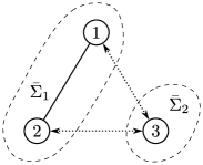
Figure 1: A multi-agent system with two clusters $I_{1}=\{1,2\}$ and $I_{2}=\{3\}$.

Example III.1

Consider a multi-agent system of three agents as described in Example II.2 and shown in Fig. 1, with STL tasks $\phi_{1}:=G_{[0,10]}(\|\mathbf{x}_{1}-\mathbf{x}_{2}\|\leq 3)$, $\phi_{2}:=F_{[5,10]}(\|\mathbf{x}_{2}-[50,20]^{\mathsf{T}}\|\leq 5)$, and $\phi_{3}:=G_{[0,10]}(\|\mathbf{x}_{3}-[20,80]^{\mathsf{T}}\|\leq 10)$. Here, $\phi_{1}$ is a collaborative task depending on agents $1$ and $2$, $\phi_{2}$ and $\phi_{3}$ are non-collaborative tasks depending on agent $2$ and $3$, respectively. The task dependency graph of the multi-agent system thus induces two maximal dependency clusters $I_{1}=\{1,2\}$ and $I_{2}=\{3\}$.

In the sequel, we construct a product system that captures the collaborative behavior of all the agents within a cluster. The product system for a cluster of agents is formally defined as follows.

Definition III.2

Consider a cluster of agents $\Sigma_{i}$, $i\in I_{k}=\{{k_{1}},\ldots,{k_{|I_{k}|}}\}$, $k\in\{1,\dots,K\}$, with each agent as described in (3). The product system for the cluster of agents denoted by $\bar{\Sigma}_{k}=\mathcal{I}(\Sigma_{k_{1}},\dots,\Sigma_{k_{|I_{k}|}})$ is a tuple $\bar{\Sigma}_{k}=(\bar{X}_{k},\bar{U}_{k},\bar{W}_{k},\bar{f}_{k},\bar{g}_{k},\bar{h}_{k})$ where

1. $\bar{X}_{k}=\prod_{i\in I_{k}}X_{i}$, $\bar{U}_{k}=\prod_{i\in I_{k}}U_{i}$, and $\bar{W}_{k}=\prod_{i\in I_{k}}W_{i}$ are the state, external input spaces, and internal input spaces, respectively;

2. $\bar{f}_{k}$ is the flow drift, $\bar{g}_{k}$ is the external input matrix, and $\bar{h}_{k}$ is the internal input matrix defined as: $\bar{f}_{k}(\bar{\mathbf{x}}_{k}(t))=[f_{k_{1}}(\mathbf{x}_{k_{1}}(t));\dots;f_{k_{|I_{k}|}}(\mathbf{x}_{k_{|I_{k}|}}(t))]$, $\bar{g}_{k}(\bar{\mathbf{x}}_{k}(t))=\textup{diag}(g_{k_{1}}(\mathbf{x}_{k_{1}}(t)),\dots,g_{k_{|I_{k}|}}(\mathbf{x}_{k_{|I_{k}|}}(t))$, $\bar{h}_{k}(\bar{\mathbf{w}}_{k}(t))=[h_{k_{1}}(\mathbf{w}_{k_{1}}(t));\dots;h_{k_{|I_{k}|}}(\mathbf{w}_{k_{|I_{k}|}}(t))],$ where $\bar{\mathbf{x}}_{k}=[\mathbf{x}_{k_{1}};\dots;\mathbf{x}_{k_{|I_{k}|}}]\in\mathbb{R}^{\bar{n}_{k}}$ with $\bar{n}_{k}={n_{k_{1}}}+\dots+{n_{k_{|I_{k}|}}}$, $\bar{\mathbf{w}}_{k}=[\mathbf{w}_{k_{1}};\dots;\mathbf{w}_{k_{|I_{k}|}}]\in\mathbb{R}^{\bar{p}_{k}}$ with $\bar{p}_{k}={p_{k_{1}}}+\dots+{p_{k_{|I_{k}|}}}$.

A trajectory of $\bar{\Sigma}_{k}$ is an absolutely continuous map $(\bar{\mathbf{x}}_{k},\bar{\mathbf{w}}_{k})\!:\!\mathbb{R}_{\geq 0}\!\rightarrow\!\bar{X}_{k}\!\times\!\bar{W}_{k}$ such that for all $t\!\geq\!0$

$$\dot{\bar{\mathbf{x}}}_{k}(t)=\bar{f}_{k}(\bar{\mathbf{x}}_{k}(t))+\bar{g}_{k}(\bar{\mathbf{x}}_{k}(t))\bar{\mathbf{u}}_{k}(t)+\bar{h}_{k}(\bar{\mathbf{w}}_{k}(t)),$$ (5)

where $\bar{\mathbf{u}}_{k}\!=[\mathbf{u}_{k_{1}};\dots;\mathbf{u}_{k_{|I_{k}|}}]$. We denote by $\mathcal{N}_{i}^{c}=I_{k}\setminus\{i\}$ the set of cooperative neighbors of each agent $\Sigma_{i}$, $i\in I_{k}$, and the cooperative internal input by the stacked state $\mathbf{z}_{i}(t)=[\mathbf{x}_{j_{1}}(t);\dots;\mathbf{x}_{j_{|I_{k}-1|}}(t)]$, with $Z_{i}=\prod_{j\in\mathcal{N}_{i}^{c}}X_{j}$. We assume for the sake of simplicity that $\mathcal{N}_{i}^{a}\cap\mathcal{N}_{i}^{c}=\emptyset$.

Note that, since an agent can only belong to one cluster, it can be shown easily that the interconnection of all the clusters forms the same multi-agent system as the interconnection of all the single agents as in Definition II.1, i.e., $\mathcal{I}(\Sigma_{1},\dots,\Sigma_{N})=\mathcal{I}(\bar{\Sigma}_{1},\dots,\bar{\Sigma}_{K})$ where $\bar{\Sigma}_{k}=\mathcal{I}(\Sigma_{k_{1}},\dots,\Sigma_{k_{|I_{k}|}})$ are the clusters in the multi-agent system.

We further define for each cluster $\bar{\Sigma}_{k}$ the STL formula as $\bar{\phi}_{k}=\land_{i=1}^{I_{k}}\phi_{i}$. If the satisfaction of $\bar{\phi}_{k}$ for each cluster $I_{k}$ is guaranteed, it holds by definition that the satisfaction of all the individual formulae $\phi_{i},i\in I_{k}$ is guaranteed as well. As defined earlier, the satisfaction of $\bar{\phi}_{k}$, $k\in\{1,\dots,K\}$, depends on the set of agents $I_{k}\subseteq I$. Note that we have by the definition of maximal dependency cluster that $I_{1}\cup\dots\cup I_{K}=I$ and $I_{k}\cap I_{k^{\prime}}=\emptyset$ for all $k,k^{\prime}\in\{1,\dots,K\}$ with $k\neq k^{\prime}$. Induced by the task dependency graph, the global STL specification can be written as $\bar{\phi}=\land_{k=1}^{K}\bar{\phi}_{k}$. Although there are no task dependencies between agents in different clusters $I_{k}$ and $I_{k^{\prime}}$, these agents might be dynamically coupled as shown in each agent’s dynamics (3) based on the interconnection graph $\mathcal{G}^{a}$. Moreover, we assume that the task dependencies are compatible with the communication graph topology of $\mathcal{G}$ as formally stated in the following.

Assumption III.3

For each $\phi_{i}$ depending on agent $\Sigma_{j}$, $j\in I$, agent $\Sigma_{i}$ can communicate with $\Sigma_{j}$, i.e., we have $\mathcal{G}^{t}\subseteq\mathcal{G}^{c}$ with $(i,j)\!\in\!E^{t}\!\implies\!(i,j)\!\in\!E^{c}$.

As mentioned in Subsection II-B, we defined the interconnection graph $\mathcal{G}^{a}=(I,E^{a})$ for the multi-agent system with each agent $\Sigma_{i}$ being a vertex in the graph. Fur future use, we further denote by a directed graph $\bar{\mathcal{G}}^{a}=(\bar{I},\bar{E}^{a})$ as the cluster interconnection graph capturing the dynamical couplings among the $K$ clusters in the multi-agent system, where $\bar{I}=\{1,\dots,K\}$, and $(j,i)\in\bar{E}^{a}$ indicate that cluster $I_{j}$ provides internal inputs to cluster $I_{i}$, i.e., $\exists j_{l}\in I_{j},i_{l^{\prime}}\in I_{i}$ such that $(j_{l},i_{l^{\prime}})\in E^{a}$.

III-B Assume-guarantee contracts for multi-agent systems

In this subsection, we introduce a notion of continuous-time assume-guarantee contracts to establish our compositional framework. A new concept of contract satisfaction is defined which is tailored to the funnel-based formulation of STL specifications as discussed in Subsection III-F.

Definition III.4

(Assume-guarantee contracts) Consider an agent $\Sigma_{i}\!=\!(X_{i},U_{i},W_{i},f_{i},g_{i},h_{i})$, and the cluster $\bar{\Sigma}_{k}$ that $\Sigma_{i}$ belongs to as in Definition III.2. An assume-guarantee contract for $\Sigma_{i}$ is a tuple $\mathcal{C}_{i}\!=\!(A_{i}^{a},G_{i})$ where

1. $A_{i}^{a}:\mathbb{R}_{\geq 0}\rightarrow W_{i}=\prod_{j\in\mathcal{N}_{i}^{a}}X_{j}$ is a set of assumptions on the adversarial internal input trajectories, i.e., the state trajectories of its adversarial neighboring agents;

2. $G_{i}:\mathbb{R}_{\geq 0}\rightarrow\bar{X}_{k}=X_{k_{1}}\times\ldots\times X_{i}\times\ldots\times X_{I_{k}}$ is a set of guarantees on the state trajectories and cooperative internal input trajectories.

We say that $\Sigma_{i}$ (weakly) satisfies $\mathcal{C}_{i}$, denoted by $\Sigma_{i}\models\mathcal{C}_{i}$, if for any trajectory $(\mathbf{x}_{i},\mathbf{w}_{i})\!:\!\mathbb{R}_{\geq 0}\!\rightarrow\!X_{i}\!\times\!W_{i}$ of $\Sigma_{i}$, the following holds: for all $t\in\mathbb{R}_{\geq 0}$, if $\mathbf{w}_{i}(s)\!\in\!A_{i}^{a}(s)$ for all $s\in[0,t]$, then we have $(\mathbf{x}_{i}(s),\mathbf{z}_{i}(s))\in G_{i}(s)$ for all $s\in[0,t]$.

We say that $\Sigma_{i}$ uniformly strongly satisfies $\mathcal{C}_{i}$, denoted by $\Sigma_{i}\models_{us}\mathcal{C}_{i}$, if for any trajectory $(\mathbf{x}_{i},\mathbf{w}_{i})\!:\!\mathbb{R}_{\geq 0}\!\rightarrow\!X_{i}\!\times\!W_{i}$ of $\Sigma_{i}$, the following holds: there exists $\delta_{i}>0$ such that for all $t\in\mathbb{R}_{\geq 0}$, if $\mathbf{w}_{i}(s)\!\in\!A_{i}^{a}(s)$ for all $s\in[0,t]$, then we have $(\mathbf{x}_{i}(s),\mathbf{z}_{i}(s))\in G_{i}(s)$ for all $s\in[0,t+\delta_{i}]$.

Note that $\Sigma_{i}\models_{us}\mathcal{C}_{i}$ implies $\Sigma_{i}\models\mathcal{C}_{i}$. An illustration of weak and strong satisfaction of a contract is depicted in Fig. 2.

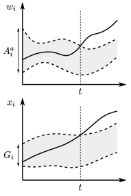
(a) Weak satisfaction.

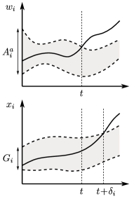
(b) Strong satisfaction.

Figure 2: An illustration of weak and strong satisfaction of a contract. Top: trajectories of the internal inputs $w_{i}$. Bottom: trajectories of the state $x_{i}$.

As it can be seen in the above definition, the set of guarantees $G_{i}$ for each agent $\Sigma_{i}$ is on both the state trajectories of $\Sigma_{i}$ and the cooperative internal input trajectories, i.e., the state trajectories of its cooperative neighbors $\Sigma_{j}$, $j\in\mathcal{N}_{i}^{c}$. For later use, let us define $\overline{\textbf{Proj}}^{i}(G_{i}(t)):=\{x_{i}\in X_{i}|\exists x_{k_{j}}\in X_{k_{j}},\forall{k_{j}}\in I_{k},\text{s.t. }[x_{k_{1}};\ldots;x_{i};\ldots;x_{k_{|}I_{k}|}]\in G_{i}(t)\}$.

It should be mentioned that multi-agent systems have no assumptions on internal inputs since they have trivial null internal input sets as in Definition II.1. Hence, an AGC for a multi-agent system $\Sigma=\mathcal{I}(\Sigma_{1},\dots,\Sigma_{N})$ will be denoted by $\mathcal{C}=(\emptyset,G)$ with $G\subseteq X$. The concept of contract satisfaction by a multi-agent system $\Sigma$ is similar to those for the single agents by removing the conditions on internal inputs:

We say that $\Sigma$ (weakly) satisfies $\mathcal{C}$, denoted by $\Sigma\models\mathcal{C}$, if for any trajectory $\mathbf{x}\!:\!\mathbb{R}_{\geq 0}\!\rightarrow\!X$ of $\Sigma$, and for all $s\in\mathbb{R}_{\geq 0}$, we have $\mathbf{x}(s)\in G(s)$.

Similarly, we can define assume-guarantee contracts for clusters of agents in the multi-agent system.

Definition III.5

Consider a cluster of agents $\bar{\Sigma}_{k}=(\bar{X}_{k},\bar{U}_{k},\bar{W}_{k},\bar{f}_{k},\bar{g}_{k},\bar{h}_{k})$ as in Definition III.2. An assume-guarantee contract for the cluster can be defined as $\bar{\mathcal{C}}_{k}\!=\!(\bar{A}_{k}^{a},\bar{G}_{k})$, where $\bar{A}_{k}^{a}:\mathbb{R}_{\geq 0}\rightarrow W_{i}=\prod_{i\in I_{k}}W_{i}$ and $\bar{G}_{k}:\mathbb{R}_{\geq 0}\rightarrow\bar{X}_{k}$.

The concept of contract satisfaction by the clusters can be defined similarly as in Definition III.4 and is provided in the Appendix in Definition .1.

The following proposition will be used to show the main compositionality result of this section.

Proposition III.6

Consider a cluster of agents $\bar{\Sigma}_{k}=\mathcal{I}(\Sigma_{k_{1}},\dots,\Sigma_{k_{|I_{k}|}})$, where each agent is associated with a local assume-guarantee contract $C_{i}\!=\!(A_{i}^{a},G_{i})$, $i\in I_{k}$. Consider the assume-guarantee contract $\bar{\mathcal{C}}_{k}\!=\!(\bar{A}_{k}^{a},\bar{G}_{k})$ for the cluster $\bar{\Sigma}_{k}$, as in Definition III.5 constructed from the local assume-guarantee contracts $\mathcal{C}_{i}$, $i\in I_{k}$ as follows: $\bar{A}_{k}^{a}=\prod_{i\in I_{k}}A_{i}^{a}$ and $\bar{G}_{k}=\cap_{i\in I_{k}}G_{i}$. Then, we have $\bar{\Sigma}_{k}\models\bar{\mathcal{C}}_{k}$ if $\Sigma_{i}\models\mathcal{C}_{i}$ for all $i\in I_{k}$; $\bar{\Sigma}_{k}\models_{us}\bar{\mathcal{C}}_{k}$ if $\Sigma_{i}\models_{us}\mathcal{C}_{i}$ for all $i\in I_{k}$.

Proof:

The proof can be found in the appendix. ∎

In the following subsections, we present our main compositionality results by providing conditions under which one can go from the satisfaction of local contracts at the agent’s level to the satisfaction of a global contract for the multi-agent system.

III-C Compositional reasoning for acyclic interconnections

In this subsection, we first present the compositionality result for multi-agent systems with acyclic interconnections among the clusters, i.e., the cluster interconnection graph is a directed acyclic graph (DAG).

Theorem III.7

Consider a multi-agent system $\Sigma=\mathcal{I}(\Sigma_{1},\dots,\Sigma_{N})$ as in Definition II.1 consisting of $K$ clusters induced by the task dependency graph. Assume that the cluster interconnection graph $\bar{\mathcal{G}}^{a}=(\bar{I},\bar{E}^{a})$ is a directed acyclic graph. Suppose each agent $\Sigma_{i}$ is associated with a contract $\mathcal{C}_{i}\!=\!(A_{i}^{a},G_{i})$. Let $\mathcal{C}=(\emptyset,G)=(\emptyset,\prod_{k\in\bar{I}}\bar{G}_{k})$ be the corresponding contract for $\Sigma$, with $\bar{G}_{k}=\cap_{i\in I_{k}}G_{i}$, $k\in\bar{I}$. Assume the following conditions hold:

1. for all $i\in I$, $\Sigma_{i}\models\mathcal{C}_{i}$;

2. for all $i\in I$, $\prod_{j\in\mathcal{N}_{i}^{a}}\overline{\textbf{Proj}}^{j}(G_{j}(t))\subseteq A_{i}^{a}(t)$ for all $t\in\mathbb{R}_{\geq 0}$.

Then, $\Sigma\models\mathcal{C}$.

Proof:

The proof can be found in the appendix. ∎

The above theorem provides us a compositionality result for multi-agent systems with acyclic cluster interconnection graphs via assume-guarantee contracts. However, we should mention that weak satisfaction is generally insufficient to reason about general networks with an interconnection graph containing cycles. Interested readers are referred to [20, Example 6] for a counter-example. A more general result is presented in the next subsection which allows us to deal with cyclic interconnections. An illustration of multi-agent systems with acyclic and cyclic cluster interconnection graphs is depicted in Fig. 3.

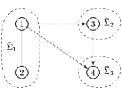
(a) Acyclic cluster interconnection graph.

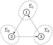
(b) Cyclic cluster interconnection graph.

Figure 3: An illustration of a multi-agent system with acyclic or cyclic cluster interconnection graphs. The solid lines indicate the communication links between agents, and the dotted lines with arrows indicate the dynamical couplings between clusters.

III-D Compositional reasoning for cyclic interconnections

Next, we present a compositionality result on multi-agent systems with possibly cyclic interconnections between the clusters.

Theorem III.8

Consider a multi-agent system $\Sigma=\mathcal{I}(\Sigma_{1},\dots,\Sigma_{N})$ as in Definition II.1 consisting of $K$ clusters induced by the task dependency graph. Suppose each agent $\Sigma_{i}$ is associated with a contract $\mathcal{C}_{i}\!=\!(A_{i}^{a},G_{i})$. Let $\mathcal{C}=(\emptyset,G)=(\emptyset,\prod_{k\in\bar{I}}\bar{G}_{k})$ be the corresponding contract for $\Sigma$, with $\bar{G}_{k}=\cap_{i\in I_{k}}G_{i}$, $k\in\bar{I}$. Assume the following conditions hold:

1. for all $i\in I$, for any trajectory $(\mathbf{x}_{i},\mathbf{w}_{i}):\mathbb{R}_{\geq 0}\rightarrow X_{i}\times W_{i}$ of $\Sigma_{i}$, $\mathbf{x}_{i}(0)\in\overline{\textbf{Proj}}^{i}(G_{i}(0))$;

2. for all $i\in I$, $\Sigma_{i}\models_{us}\mathcal{C}_{i}$;

3. for all $i\in I$, $\prod_{j\in\mathcal{N}_{i}^{a}}\overline{\textbf{Proj}}^{j}(G_{j}(t))\subseteq A_{i}^{a}(t)$ for all $t\in\mathbb{R}_{\geq 0}$.

Then, $\Sigma\models\mathcal{C}$.

Proof:

The proof can be found in the appendix. ∎

The above theorem presents a compositionality result that works for multi-agent systems with both acyclic and cyclic cluster interconnection graphs due to the fact that $\Sigma_{i}\models_{us}\mathcal{C}_{i}$ implies $\Sigma_{i}\models\mathcal{C}_{i}$.

Remark III.9

It is important to note that while in the definition of the strong contract satisfaction in [20] the parameter $\delta$ may depend on time, our definition of assume-guarantee contracts requires a uniform $\delta$ for all time. The reason for this choice is that the uniformity of $\delta$ is critical in our compositional reasoning, since we do not require the set of guarantees to be closed as in [20]. See [20, Example 9] for an example, showing that the compositionality result does not hold using the concept of strong satisfaction when the set of guarantees of the contract is open. Indeed, as it will be shown in the next section, the set of guarantees of the considered contracts are open and one will fail to provide a compositionality result based on the classical (non-uniform) notion of strong satisfaction in [20].

III-E From weak to strong satisfaction of contacts

Now, we provide an important result in Proposition III.11 to be used to prove the main theorem in next section, which shows how to go from weak to uniform strong satisfaction of AGCs by relaxing the assumptions. The following notion of $\varepsilon$-closeness of trajectories is needed to measure the distance between continuous-time trajectories.

Definition III.10

([43], $\varepsilon$-closeness of trajectories) Let $Z\subseteq\mathbb{R}^{n}$. Consider $\varepsilon>0$ and two continuous-time trajectories $z_{1}:\mathbb{R}_{\geq 0}\rightarrow Z$ and $z_{2}:\mathbb{R}_{\geq 0}\rightarrow Z$. Trajectory $z_{2}$ is said to be $\varepsilon$-close to $z_{1}$, if for all $t_{1}\in\mathbb{R}_{\geq 0}$, there exists $t_{2}\in\mathbb{R}_{\geq 0}$ such that $|t_{1}-t_{2}|\leq\varepsilon$ and $\|z_{1}(t_{1})-z_{2}(t_{2})\|\leq\varepsilon$. We define the $\varepsilon$-expansion of $z_{1}$ by : $\mathcal{B}_{\varepsilon}(z_{1})=\{z^{\prime}:\mathbb{R}_{\geq 0}\rightarrow Z\mid z^{\prime}\text{ is }\varepsilon\text{-close to }z_{1}\}$. For set $A=\{z:\mathbb{R}_{\geq 0}\rightarrow Z\}$, $\mathcal{B}_{\varepsilon}(A)=\cup_{z\in A}\mathcal{B}_{\varepsilon}(z)$.

Now, we introduce the following proposition which will be used later to prove our main theorem.

Proposition III.11

(From weak to uniformly strong satisfaction of AGCs) Consider an agent $\Sigma_{i}=(X_{i},U_{i},W_{i},f_{i},g_{i},h_{i})$ associated with a local AGC $\mathcal{C}_{i}\!=\!(A_{i}^{a},G_{i})$. If trajectories of $\Sigma_{i}$ are uniformly continuous and if there exists an $\varepsilon>0$ such that $\Sigma_{i}\models\mathcal{C}_{i}^{\varepsilon}$ with $\mathcal{C}_{i}^{\varepsilon}=(\mathcal{B}_{\varepsilon}(A_{i}^{a}),G_{i})$, then $\Sigma_{i}\models_{us}\mathcal{C}_{i}$.

Proof:

The proof can be found in the appendix. ∎

In the next subsection, we show how to cast STL formulae into time-varying funnel functions which will be leveraged later to design continuous-time assume-guarantee contracts.

III-F Casting STL as funnel functions

In this work, each agent in the multi-agent system is subject to an STL task $\phi_{i}$ which does not only depend on the behavior of agent $\Sigma_{i}$, but also on other agents $\Sigma_{j}$, $j\in I$. Let us denote by $I_{\phi_{i}}=\{i_{1},\ldots,i_{|P_{i}|}\}$ the set of agents that are involved in $\phi_{i}$, where $P_{i}$ indicates the total number of agents that are involved in $\phi_{i}$. We further define $\mathbf{x}_{\phi_{i}}(t)=[\mathbf{x}_{i_{1}}(t);\ldots;\mathbf{x}_{i_{|P_{i}|}}(t)]\in\mathbb{R}^{n_{P_{i}}}$, where $n_{P_{i}}:=n_{i_{1}}+\ldots+n_{i_{|P_{i}|}}$.

In order to formulate the STL tasks as assume-guarantee contracts, we first show in this subsection how to cast STL formulae into funnel functions. Note that the idea of casting STL as funnel functions was originally proposed in [29].

First, let us define a funnel function $\gamma_{i}(t)=(\gamma_{i}^{0}-\gamma_{i}^{\infty})\exp(-l_{i}t)+\gamma_{i}^{\infty}$, where $l_{i},t\in\mathbb{R}_{\geq 0}$, $\gamma_{i}^{0},\gamma_{i}^{\infty}\in\mathbb{R}_{>0}$ with $\gamma_{i}^{0}\geq\gamma_{i}^{\infty}$. Consider the robust semantics of STL introduced in Subsection II-A. For each agent with STL specification $\phi_{i}$ in (2) with the corresponding non-temporal formula $\psi_{i}$ inside the $F,G,FG$ operators as in (2), we can achieve $0<r_{i}\leq\rho_{i}^{\phi_{i}}(\mathbf{x}_{\phi_{i}},0)\leq\rho_{i}^{max}$ by prescribing a temporal behavior to $\rho_{i}^{\psi_{i}}(\mathbf{x}_{\phi_{i}}(t))$ through a properly designed function $\gamma_{i}$ and parameter $\rho_{i}^{max}$, and the funnel

$$-\gamma_{i}(t)+\rho_{i}^{max}<\rho_{i}^{\psi_{i}}(\mathbf{x}_{\phi_{i}}(t))<\rho_{i}^{max}$$

$$\iff-\gamma_{i}(t)<\rho_{i}^{\psi_{i}}(\mathbf{x}_{\phi_{i}}(t))-\rho_{i}^{max}<0.$$ (6)

Note that functions $\gamma_{i}:\mathbb{R}_{\geq 0}\rightarrow\mathbb{R}_{>0}$, $i\in\{1,\ldots,N\}$, are positive, continuously differentiable, bounded, and non-increasing [44]. The design of $\gamma_{i}$ and $\rho_{i}^{max}$ that leads to the satisfaction of $0<r_{i}\leq\rho_{i}^{\phi_{i}}(\mathbf{x}_{\phi_{i}},0)\leq\rho_{i}^{max}$ through (6) will be discussed in Remark IV.6 in Section IV-A.

To better illustrate the satisfaction of STL tasks using funnel-based strategy, we provide the next example with more intuitions.

Example III.12

(a) Funnel $(-\gamma_{1}(t)+\rho_{1}^{max},\rho_{1}^{max})$ (dashed lines) for $\phi_{1}:=F_{[0,8]}\psi_{1}$, s.t. $\rho_{1}^{\phi_{1}}(\mathbf{x},0)\geq r_{1}$ with $r_{1}=0.1$ (dotted line).

(b) Funnel $(-\gamma_{2}(t)+\rho_{2}^{max},\rho_{2}^{max})$ (dashed lines) for $\phi_{2}:=G_{[0,8]}\psi_{2}$, s.t. $\rho_{2}^{\phi_{2}}(\mathbf{x},0)\geq r_{2}$ with $r_{2}=0.1$ (dotted line).

Figure 4: Funnels for STL formulae.

Consider STL formulae $\phi_{1}:=F_{[0,8]}\psi_{1}$ and $\phi_{2}:=G_{[0,8]}\psi_{2}$ with $\psi_{1}=\mu_{1}$ and $\psi_{2}=\mu_{2}$, where $\mu_{1}$ and $\mu_{2}$ are associated with predicate functions $\mathcal{P}_{1}(\mathbf{x})=\mathcal{P}_{2}(\mathbf{x})=\mathbf{x}$. Figs. 4(a) and 4(b) show the funnel in (6) prescribing a desired temporal behavior to satisfy $\phi_{1}$ and $\phi_{2}$, respectively. Specifically, it can be seen that $\rho_{1}^{\psi_{1}}(\mathbf{x}(t))\in(-\gamma_{1}(t)+\rho_{1}^{max},\rho_{1}^{max})$ and $\rho_{2}^{\psi_{1}}(\mathbf{x}(t))\in(-\gamma_{2}(t)+\rho_{2}^{max},\rho_{2}^{max})$ for all $t\in\mathbb{R}_{\geq 0}$ as in Fig. 4. This shows that (6) is satisfied for all $t\in\mathbb{R}_{\geq 0}$. Then, the connection between atomic formulae $\rho_{i}^{\psi_{i}}(\mathbf{x}(t))$ and temporal formulae $\rho_{i}^{\phi_{i}}(\mathbf{x},0)$, is made by the choice of $\gamma_{1}$, $\gamma_{2}$, $\rho_{1}^{max}$, and $\rho_{2}^{max}$. For example, the lower funnel $-\gamma_{1}(t)+\rho_{1}^{max}$ in Fig. 4(a) ensures that $\rho_{1}^{\psi_{1}}(\mathbf{x}(t))\geq r_{1}=0.1$ for all $t\geq 6$, which guarantees that the STL task $\phi_{1}$ is robustly satisfied by $\rho_{1}^{\phi_{1}}(\mathbf{x},0)\geq r_{1}$.

In the sequel, STL tasks will be formulated as contracts by leveraging the above-presented funnel-based framework. We will then design local controllers enforcing the local contracts over the agents (cf. Section IV, Theorem IV.5).

III-G From STL tasks to assume-guarantee contracts

The objective of the paper is to synthesize local controllers $\mathbf{u}_{i}$, for agents $\Sigma_{i}$ to achieve the global STL specification $\phi$, where $\phi=\land_{i=1}^{N}\phi_{i}$ and $\phi_{i}$ is the STL task of $\Sigma_{i}$. Hence, in view of the interconnection between the agents and the distributed nature of the local controllers, one has to make some assumptions on the behaviour of the neighbouring components while synthesizing the local controllers. This property can be formalized in terms of contracts, where the contract should reflect the fact that the objective is to ensure that agent $\Sigma_{i}$ satisfies “the guarantee” $\phi_{i}$ under “the assumption” that: each of the adversarial neighboring agents $\Sigma_{j}$, satisfies its local task $\phi_{j}$, $j\in\mathcal{N}_{i}^{a}$. In this context, and using the concept of funnel function to cast the STL tasks as presented in Section III-F, a natural assignment of the local assume-guarantee contract $\mathcal{C}_{i}\!=\!(A_{i}^{a},G_{i})$ for the agents $\Sigma_{i}$, can be defined formally as follows:

1. $A_{i}^{a}=\prod_{j\in\mathcal{N}_{i}^{a}}\{\mathbf{x}_{j}:\mathbb{R}_{\geq 0}\rightarrow X_{j}\mid-\gamma_{j}(t)+\rho_{j}^{max}<\rho_{j}^{\psi_{j}}(\mathbf{x}_{\phi_{j}}(t))<\rho_{j}^{max},\forall t\in\mathbb{R}_{\geq 0}\}$;

2. $G_{i}=\{(\mathbf{x}_{i},\mathbf{z}_{i}):\mathbb{R}_{\geq 0}\rightarrow X_{i}\times Z_{i}\mid-\gamma_{i}(t)+\rho_{i}^{max}<\rho_{i}^{\psi_{i}}({\mathbf{x}}_{\phi_{i}}(t))<\rho_{i}^{max},\forall t\in\mathbb{R}_{\geq 0}\}$;

where $-\gamma,\rho^{\psi},\rho^{max}$ are the functions discussed in Subsection III-F corresponding to their STL tasks.

Once the specification $\phi$ is decomposed into local contracts and in view of Theorems III.7 and III.8, Problem II.3 can be solved by considering local control problems for each agent $\Sigma_{i}$. These control problems can be solved in a distributed manner and are formally defined as follows:

Problem III.13

Given an agent $\Sigma_{i}=(X_{i},U_{i},W_{i},f_{i},g_{i},h_{i})$ associated with an assume-guarantee contract $\mathcal{C}_{i}\!=\!(A_{i}^{a},G_{i})$, where $A_{i}^{a}$, and $G_{i}$ are given by STL formulae by means of funnel functions, synthesize a local controller $\mathbf{u}_{i}:\bar{X}_{k}\times\mathbb{R}_{\geq 0}\rightarrow U_{i}$ such that $\Sigma_{i}\models_{us}\mathcal{C}_{i}$.

IV Distributed Controller Design

In this section, we first provide a solution to Problem III.13 by designing controllers ensuring that local contracts for agents are uniformly strongly satisfied. Then, we show that based on our compositionality result proposed in the last section, the global STL task for the network is satisfied by applying the derived local controllers to agents individually.

First, we utilize the idea of funnel-based control (a.k.a prescribed performance control) [44] in order to enforce the satisfaction of local contracts by prescribing certain transient behavior of the funnels that constrain the closed-loop trajectories of the agents.

IV-A Local controller design

As discussed in Subsection III-F, one can enforce STL tasks via funnel-based strategy by prescribing the transient behavior of $\rho_{i}^{\psi_{i}}(\mathbf{x}_{\phi_{i}}(t))$ within the predefined region in

$$-\gamma_{i}(t)<\rho_{i}^{\psi_{i}}(\mathbf{x}_{\phi_{i}}(t))-\rho_{i}^{max}<0,$$ (7)

where $\psi_{i}$ is the corresponding non-temporal formula inside the $F,G,FG$ operators as in (2). In order to leverage the idea of funnel-based control to achieve this, an error term is first defined for each $\rho_{i}^{\psi_{i}}(\mathbf{x}_{\phi_{i}}(t))$ as $e_{i}(\mathbf{x}_{\phi_{i}}(t))=\rho_{i}^{\psi_{i}}(\mathbf{x}_{\phi_{i}}(t))-\rho_{i}^{max}$. We can then obtain the modulated error as $\hat{e}_{i}(\mathbf{x}_{\phi_{i}},t)=\frac{e_{i}(\mathbf{x}_{\phi_{i}}(t))}{\gamma_{i}(t)}$ and the prescribed performance region $\hat{\mathcal{D}_{i}}:=(-1,0)$. The transformed error is then defined as

$$\epsilon_{i}({\mathbf{x}}_{\phi_{i}},t):=T_{i}(\hat{e}_{i}(\mathbf{x}_{\phi_{i}},t))=\ln(-\frac{\hat{e}_{i}(\mathbf{x}_{\phi_{i}},t)+1}{\hat{e}_{i}(\mathbf{x}_{\phi_{i}},t)}).$$ (8)

The basic idea of funnel-based control is to derive a control policy such that $\epsilon_{i}({\mathbf{x}}_{\phi_{i}},t)$ is rendered bounded, which implies the satisfaction of (7). A more detailed description of the funnel-based strategy is provided in the Appendix -A.

We make the following two assumptions on functions $\rho_{i}^{\psi_{i}}$ for formulae $\psi_{i}$, which are required for the local controller design in the main result of this section.

Assumption IV.1

Each formula within class $\psi$ as in (1) has the following properties: (i) $\rho_{i}^{\psi_{i}}:\mathbb{R}^{n_{i}}\rightarrow\mathbb{R}$ is concave and (ii) the formula is well-posed in the sense that for all $C\in\mathbb{R}$ there exists $\bar{C}\geq 0$ such that for all $\mathbf{x}_{\phi_{i}}\in\mathbb{R}^{n_{P_{i}}}$ with $\rho_{i}^{\psi_{i}}(\mathbf{x}_{\phi_{i}})\geq C$, one has $\|\mathbf{x}_{\phi_{i}}\|\leq\bar{C}<\infty$.

Define the global maximum of $\rho_{i}^{\psi_{i}}(\mathbf{x}_{\phi_{i}})$ as $\rho_{i}^{opt}=\sup_{\mathbf{x}_{\phi_{i}}\in\mathbb{R}^{n_{P_{i}}}}\rho_{i}^{\psi_{i}}(\mathbf{x}_{\phi_{i}})$.

Assumption IV.2

The global maximum of $\rho_{i}^{\psi_{i}}(\mathbf{x}_{\phi_{i}})$ is positive, and $\frac{\partial\rho_{i}^{\psi_{i}}({\mathbf{x}}_{\phi_{i}})}{\partial\mathbf{x}_{i}}$ is a non-zero vector.

Note that the above assumption implies that $\psi_{i}$ and hence $\phi_{i}$ is locally feasible. The assumption on $\frac{\partial\rho_{i}^{\psi_{i}}({\mathbf{x}}_{\phi_{i}})}{\partial\mathbf{x}_{i}}$ being a non-zero vector is used to avoid local optima which can cause infeasibility issues. One can design proper funnel parameters such that the local optima are avoided.

The following assumptions are required on agents and the task dependency graphs of multi-agent systems in order to design controllers enforcing local contracts.

Assumption IV.3

Consider agent $\Sigma_{i}$ as in (3). The functions $f_{i}:\mathbb{R}^{n_{i}}\rightarrow\mathbb{R}^{n_{i}}$, $g_{i}:\mathbb{R}^{n_{i}}\rightarrow\mathbb{R}^{n_{i}\times m_{i}}$, and $h_{i}:\mathbb{R}^{p_{i}}\rightarrow\mathbb{R}^{n_{i}}$ are locally Lipschitz continuous, and $g_{i}(\mathbf{x}_{i})g_{i}(\mathbf{x}_{i})^{\top}$ is positive definite for all $\mathbf{x}_{i}\in\mathbb{R}^{n_{i}}$.

Assumption IV.4

The task dependency graph $\mathcal{G}^{t}=(I,E^{t})$ of the multi-agent system is a directed acyclic graph.

Now, we are ready to present the main result of this section solving Problem III.13 for the local controller design.

Theorem IV.5

Consider an agent $\Sigma_{i}$ as in (3) belonging to cluster $\bar{\Sigma}_{k}$ and satisfying Assumption IV.3. Given that $\Sigma_{i}$ is subject to STL task $\phi_{i}$, and is associated with its local assume-guarantee contract $\mathcal{C}_{i}\!=\!(A_{i}^{a},G_{i})$, where

1. $A_{i}^{a}=\prod_{j\in\mathcal{N}_{i}^{a}}\{\mathbf{x}_{j}:\mathbb{R}_{\geq 0}\rightarrow X_{j}\mid-\gamma_{j}(t)+\rho_{j}^{max}<\rho_{j}^{\psi_{j}}(\mathbf{x}_{\phi_{j}}(t))<\rho_{j}^{max},\forall t\in\mathbb{R}_{\geq 0}\}$;

2. $G_{i}=\{(\mathbf{x}_{i},\mathbf{z}_{i}):\mathbb{R}_{\geq 0}\rightarrow X_{i}\times Z_{i}\mid-\gamma_{i}(t)+\rho_{i}^{max}<\rho_{i}^{\psi_{i}}({\mathbf{x}}_{\phi_{i}}(t))<\rho_{i}^{max},\forall t\in\mathbb{R}_{\geq 0}\}$;

where $\psi_{i}$ is an atomic formula as in (1) satisfying Assumptions IV.1-IV.2. Assume $-\gamma_{i}(0)\!+\!\rho_{i}^{max}\!<\!\rho_{i}^{\psi_{i}}({\mathbf{x}}_{\phi_{i}}(0))\!<\!\rho_{i}^{max}\!<\!\rho_{i}^{opt}$, for all $i\in I_{k}$. If Assumption IV.4 holds, and all agents $\Sigma_{i}$ in the cluster apply the controller

$${{\color[rgb]{0,0,0}{\bf}\mathbf{u}_{i}(\bar{\mathbf{x}}_{k},t)\!=\!-g_{i}^{\top}(\mathbf{x}_{i})\!\sum_{j\in I_{k}}(\frac{\partial\rho_{j}^{\psi_{j}}({\mathbf{x}}_{\phi_{j}})}{\partial\mathbf{x}_{i}}\mathcal{J}_{j}(\hat{e}_{j},t)\epsilon_{j}({\mathbf{x}}_{\phi_{j}},t)),\!\!\!}}$$ (9)

then we have $\Sigma_{i}\models_{us}\mathcal{C}_{i}$ for all $i\in I_{k}$.

Proof:

The proof can be found in the appendix. ∎

Remark IV.6

(Funnel design) Remark that the connection between atomic formulae $\rho_{i}^{\psi_{i}}(\mathbf{x}_{\phi_{i}}(t))$ and temporal formulae $\rho_{i}^{\phi_{i}}(\mathbf{x}_{\phi_{i}},0)$ is made by $\gamma_{i}$ and $\rho_{i}^{max}$ as in (6), which need to be designed as instructed in [29]. Specifically, if Assumption IV.2 holds, select

$$\small t_{i}^{\ast}\in \begin{cases}a_{i}&\text{if}\ \phi_{i}=G_{[a_{i},b_{i}]}\psi_{i}\\ {[}a_{i},b_{i}]&\text{if}\ \phi_{i}=F_{[a_{i},b_{i}]}\psi_{i}\\ {[}\underline{a}_{i}+\bar{a}_{i},\underline{b}_{i}+\bar{a}_{i}]\!&\text{if}\ \phi_{i}=F_{[\underline{a}_{i},\underline{b}_{i}]}G_{[\bar{a}_{i},\bar{b}_{i}]}\psi_{i}\end{cases}$$ (10)

$$\rho_{i}^{\max}\in \left(\max(0,\rho_{i}^{\psi_{i}}(\mathbf{x}_{\phi_{i}}(0))),\rho_{{i}}^{\text{opt}}\right)$$ (11)

$$r_{i}\in (0,\rho_{i}^{\max})$$ (12)

$$\small\gamma_{i}^{0}\in \begin{cases}(\rho_{i}^{\max}-\rho_{i}^{\psi_{i}}(\mathbf{x}_{\phi_{i}}(0)),\infty)\ &\text{if}\ t_{i}^{\ast}>0\\ (\rho_{i}^{\max}-\rho_{i}^{\psi_{i}}(\mathbf{x}_{\phi_{i}}(0)),\rho_{i}^{\max}-r_{i}]\ &\text{else}\end{cases}$$ (13)

$$\gamma_{i}^{\infty}\in \left.\left(0,\min(\gamma_{i}^{0},\rho_{i}^{\max}-r_{i})\right]\right.$$ (14)

$$l_{i}\in \begin{cases}\mathbb{R}_{\geq 0}&\text{if}-\gamma_{i}^{0}+\rho_{i}^{\max}\geq r_{i}\\ \frac{-\ln\left(\frac{r_{i}+\gamma_{i}^{\infty}-\rho_{i}^{\max}}{-\gamma_{i}^{0}+\gamma_{i}^{\infty}}\right)}{t_{i}^{\ast}}&\text{else}.\end{cases}$$ (15)

With $\gamma_{i}$ and $\rho_{i}^{max}$ chosen properly (as shown above), one can achieve $0\!<\!r_{i}\!\leq\!\rho_{i}^{\phi_{i}}(\mathbf{x}_{\phi_{i}},0)\!\leq\!\rho_{i}^{max}$ by prescribing a temporal behavior to $\rho_{i}^{\psi_{i}}(\mathbf{x}_{\phi_{i}}(t))$ as in the set of guarantees $G_{i}$ in Theorem IV.5, i.e., $-\gamma_{i}(t)\!+\!\rho_{i}^{max}\!<\!\rho_{i}^{\psi_{i}}(\mathbf{x}_{\phi_{i}}(t))\!<\!\rho_{i}^{max}$ for all $t\!\geq\!0$.

IV-B Global task satisfaction

Here, we show that by applying the local controllers to the agents, the global STL task for the multi-agent system is also satisfied based on our compositionality result.

Corollary IV.7

Consider a multi-agent system $\Sigma=\mathcal{I}(\Sigma_{1},\dots,\Sigma_{N})$ as in Definition II.1 consisting of $K$ clusters induced by the task dependency graph. Suppose each agent $\Sigma_{i}$ is associated with a contract $\mathcal{C}_{i}\!=\!(A_{i}^{a},G_{i})$, and each cluster of agents is associated with a contract $\bar{\mathcal{C}}_{k}\!=\!(\bar{A}_{k}^{a},\bar{G}_{k})$ as in Definition III.5. If we apply the controllers as in (9) to agents $\Sigma_{i}$, then we get $\Sigma\models\mathcal{C}=(\emptyset,\prod_{k\in\bar{I}}\bar{G}_{k})$. This means that the control objective in Problem II.3 is achieved, i.e., system $\Sigma$ satisfies signal temporal logic task $\bar{\phi}$.

Proof:

The proof can be found in the appendix. ∎

V Case Study

We demonstrate the effectiveness of the proposed results on two case studies: a room temperature regulation and a mobile multi-robot control problem.

V-A Room Temperature Regulation

Here, we apply our results to the temperature regulation of a circular building with $N=1000$ rooms each equipped with a heater, as depicted in Fig. 5. The evolution of the temperature of the interconnected model is described by the differential equation:

$$\Sigma:\dot{\mathbf{T}}(t)= A\mathbf{T}(t)+\alpha_{h}T_{h}\nu(t)+\alpha_{e}T_{e},$$ (16)

adapted from [46], where $A\!\in\!\mathbb{R}^{N\!\times\!N}$ is a matrix with elements $\{A\}_{ii}\!=\!(-\!2\alpha\!-\!\alpha_{e}\!-\!\alpha_{h}\nu_{i})$, $\{A\}_{i,i+1}\!=\!\{A\}_{i+1,i}\!=\{A\}_{1,N}\!=\!\{A\}_{N,1}=\!\alpha$, $\forall i\in\{1,\dots,N-1\}$, and all other elements are identically zero, $\mathbf{T}(k)\!=\![\mathbf{T}_{1}(k);\dots;\mathbf{T}_{N}(k)]$, $T_{e}\!=\![T_{e1};\dots;T_{eN}]$, $\nu(k)\!=\![\nu_{1}(k);\dots;\nu_{N}(k)]$, where $\nu_{i}(k)\!\in\![0,1]$, $\forall i\!\in\!\{1,\dots,N\}$, represents the ratio of the heater valve being open in room $i$. Parameters $\alpha\!=\!0.05$, $\alpha_{e}\!=\!0.008$, and $\alpha_{h}\!=\!0.0036$ are heat exchange coefficients, $T_{ei}\!=\!-1\,^{\circ}C$ is the external environment temperature, and $T_{h}\!=\!50\,^{\circ}C$ is the heater temperature.

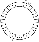
Figure 5: A circular building with $N$ rooms.

Now, by introducing $\Sigma_{i}$ described by

$$\Sigma_{i}:\dot{\mathbf{T}}_{i}(t)=a\mathbf{T}_{i}(t)+d\mathbf{w}_{i}(t)+\alpha_{h}T_{h}\nu_{i}(t)+\alpha_{e}T_{ei},$$

where $a=-\!2\alpha\!-\!\alpha_{e}\!-\!\alpha_{h}\nu_{i}$, $d=\alpha$, and $\mathbf{w}_{i}(t)=[\mathbf{T}_{i-1}(t);\mathbf{T}_{i+1}(t)]$ (with $\mathbf{T}_{0}=\mathbf{T}_{N}$ and $\mathbf{T}_{N+1}=\mathbf{T}_{1}$), one can readily verify that $\Sigma=\mathcal{I}(\Sigma_{1},\dots,\Sigma_{N})$ as in Definition II.1. The initial temperatures of these rooms are, respectively, $\mathbf{T}_{1}(0)=19\,^{\circ}C$, $\mathbf{T}_{2}(0)=25\,^{\circ}C$, $\mathbf{T}_{i}(0)=25\,^{\circ}C$ if $i\in\{i\text{ is odd }|i\in\{3,\dots,N\}\}$, and $\mathbf{T}_{i}(0)=31\,^{\circ}C$ if $i\in\{i\text{ is even }|i\in\{4,\dots,N\}\}$.

The room temperatures are subject to the following STL tasks $\phi_{1}$: $F_{[0,5]}G_{[10,20]}(\|\mathbf{T}_{1}-\mathbf{T}_{999}\|\leq 2)\wedge(\|\mathbf{T}_{1}-\mathbf{T}_{3}\|\leq 2)\wedge(\|\mathbf{T}_{1}-23\|\leq 0.5)$, $\phi_{2}$: $F_{[0,5]}G_{[10,20]}(\|\mathbf{T}_{2}-\mathbf{T}_{1000}\|\leq 2)\wedge(\|\mathbf{T}_{2}-\mathbf{T}_{4}\|\leq 2)\wedge(\|\mathbf{T}_{2}-29\|\leq 0.5)$, $\phi_{i}$: $F_{[0,5]}G_{[10,20]}(\|\mathbf{T}_{i}-\mathbf{T}_{i+2}\|\leq 2)$, for $i\in\{3,\ldots,N-2\}$, and $\phi_{N-1}$: $F_{[0,5]}G_{[10,20]}(\|\mathbf{T}_{N-1}-23\|\leq 0.5)$, and $\phi_{N}$: $F_{[0,5]}G_{[10,20]}(\|\mathbf{T}_{N}-29\|\leq 0.5)$. Intuitively, the STL tasks require the controllers (heaters) to be synthesized such that the temperature of every other rooms should eventually get close to each other, and the temperature of the rooms reach the specified region ($[22.5,23.5]$ for rooms $\Sigma_{1}$ and $\Sigma_{N-1}$, or $[28.5,29.5]$ for rooms $\Sigma_{2}$ and $\Sigma_{N}$) and remains there in the desired time slots. In this setting, the circular building consists of two clusters: $I_{1}=\{i\text{ is odd }|i\in\{1,\dots,N\}\}$ and $I_{2}=\{i\text{ is even }|i\in\{1,\dots,N\}\}$. The cluster interconnection graph is cyclic due to the dynamical couplings between the neighboring rooms.

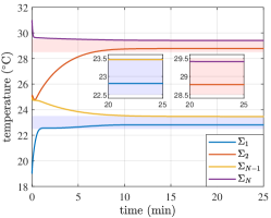
Figure 6: Trajectories of the temperature of the closed-loop agents $\Sigma_{1}$, $\Sigma_{2}$, $\Sigma_{N-1}$ and $\Sigma_{N}$, where $N=1000$, under control policy in (9).

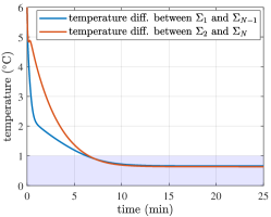
Figure 7: Trajectories of the temperature difference between the closed-loop agents $\Sigma_{1}$ and $\Sigma_{N-1}$, and between $\Sigma_{2}$ and $\Sigma_{N}$, where $N=1000$, under control policy in (9).

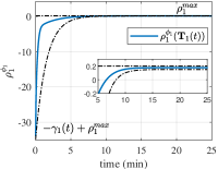
(a) Funnel for task $\phi_{1}$

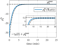
(b) Funnel for task $\phi_{2}$

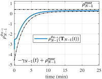
(c) Funnel for task $\phi_{N-1}$

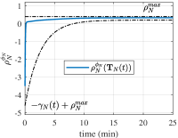
(d) Funnel for task $\phi_{N}$

Figure 8: Funnels for the STL tasks for agents $\Sigma_{1}$, $\Sigma_{2}$, $\Sigma_{N-1}$ and $\Sigma_{N}$, where $N=1000$. Performance bounds are indicated by dashed lines. Evolution of the prescribed performance of $\rho_{i}^{\phi_{i}}(\mathbf{T}_{i}(t))$ are depicted using solid lines.

To enforce the STL tasks on this large-scale multi-agent system, we apply the proposed compositional framework by leveraging the results in Theorem III.8 and applying the proposed funnel-based feedback controllers as in (9). Note that Assumptions IV.1-IV.3 on the STL formulae and the system dynamics are satisfied, and the task dependency graph also satisfies Assumption IV.4. We can thus apply the feedback controller as in (9) on the agents to enforce STL tasks in a distributed manner. Numerical implementations were performed using MATLAB on a computer with a processor Intel Core i7 3.6 GHz CPU. Note that the computation of local controllers took on average less than 0.1 ms, which is negligible. The computation cost is very cheap since the local controller $\boldsymbol{u}_{i}$ is given by a closed-form expression and computed in a distributed manner. The simulation results for agents $\Sigma_{1}$, $\Sigma_{2}$, $\Sigma_{N-1}$ and $\Sigma_{N}$ are shown in Figs. 6-8. The state trajectories of the closed-loop agents are depicted in Fig. 6. The shaded areas represent the desired temperature regions to be reached by the systems. Fig. 7 showcases the temperature difference between rooms $\Sigma_{1}$ and $\Sigma_{N-1}$, and between rooms $\Sigma_{2}$ and $\Sigma_{N}$. As can be seen from Figs. 6 and 7, all these agents satisfy their desired STL tasks. In Fig. 8, we present the temporal behaviors of $\rho_{i}^{\psi_{i}}(\mathbf{T}_{1}(t))$ for the four rooms $\Sigma_{1}$, $\Sigma_{2}$, $\Sigma_{N-1}$ and $\Sigma_{N}$. It can be readily seen that the prescribed performances of $\rho_{i}^{\psi_{i}}(\mathbf{T}_{i}(t))$ are satisfied with respect to the error funnels, which shows that the time bounds are also respected. Remark that the design parameters of the funnels are chosen according to the instructions listed in (10)-(15), which guarantees the satisfaction of temporal formulae $\rho_{i}^{\phi_{i}}(\mathbf{T}_{i},0)$ by prescribing temporal behaviors of atomic formulae $\rho_{i}^{\psi_{i}}(\mathbf{T}_{i}(t))$ as in Fig. 8. We can conclude that all STL tasks are satisfied within the desired time interval.

Note that the proposed compositional framework allows us to deal with multi-agent systems in a distributed manner, thus rendering the controller synthesis problem of large-scale multi-agent systems tractable. Moreover, the proposed local controller allows us to deal with STL tasks that not only depends on single agents but may also depend on multiple agents. Unlike the methods in [30] which require all agents in a cluster to be subject to the same STL task, our designed local controllers can handle different STL tasks in the same cluster. Therefore, the methods in [30], cannot be applied to deal with the considered problem in this paper.

V-B Mobile Robot Control

In this subsection, we demonstrate the effectiveness of the proposed results on a network of $N=5$ mobile robots, where the dynamic of each robot is adapted from [47] with induced dynamical couplings. Each mobile robot has three omni-directional wheels. The dynamics of each robot $\Sigma_{i}$, $i\in\{1,2,\ldots,5\}$ can be described by

$$\Sigma_{i}:\dot{\boldsymbol{x}}_{{i}}\!=\!A_{i}\left(B_{i}^{\top}\right)^{-1}\!\!R_{i}\boldsymbol{u}_{i}\!-\!\!f_{i}(\boldsymbol{x}),$$

where the state variable of each robot is defined as $\boldsymbol{x}_{i}:=[x_{i,1};x_{i,2};x_{i,3}]$ with $\boldsymbol{p}_{i}:=[x_{i,1};x_{i,2}]$ indicating the robot position and state $x_{i,3}$ indicating the robot orientation with respect to the $x_{i,1}$-axis; $R_{i}:=0.02$ m is the wheel radius of each robot; $A_{i}:=\begin{bmatrix}\cos(x_{i,3})\!&\!-\sin(x_{i,3})\!&\!0\\ \sin(x_{i,3})\!&\!\cos(x_{i,3})\!&\!0\\ 0\!&\!0\!&\!1\end{bmatrix}$, and $B_{i}:=\begin{bmatrix}0&\cos(\pi/6)&-\cos(\pi/6)\\ -1&\sin(\pi/6)&-\sin(\pi/6)\\ L_{i}&L_{i}&L_{i}\end{bmatrix}$ describes geometrical constraints with $L_{i}:=0.2$ m being the radius of the robot body; the term $f_{i}(\boldsymbol{x})=\sum_{j\in\mathcal{N}_{i}}k_{i}\frac{[\boldsymbol{p}_{i}-\boldsymbol{p}_{j};0]}{\|\boldsymbol{p}_{i}-\boldsymbol{p}_{j}\|+0.00001}$ is the induced dynamical coupling between agents that is used for the sake of collision avoidance, where $\boldsymbol{x}=[\boldsymbol{x}_{1};\ldots;\boldsymbol{x}_{N}]$, $k_{i}=0.1$, and $\boldsymbol{p}_{j}$, $j\in\mathcal{N}_{i}^{a}$, are the positions of $\Sigma_{i}$’s adversarial neighboring agents with $\mathcal{N}_{2}^{a}=\{4\}$, $\mathcal{N}_{3}^{a}=\{4,5\}$, $\mathcal{N}_{4}^{a}=\{2,3\}$, $\mathcal{N}_{5}^{a}=\{3\}$. Each element of the input vector $\boldsymbol{u}_{i}$ corresponds to the angular rate of one wheel. The initial states of the robots are, respectively, $\boldsymbol{x}_{1}(0)=[2;2;-\pi/4]$, $\boldsymbol{x}_{2}(0)=[4;0;0]$, $\boldsymbol{x}_{3}(0)=[6;2;\pi/4]$, $\boldsymbol{x}_{4}(0)=[8;0;0]$, $\boldsymbol{x}_{5}(0)=[10;2;-\pi/4]$.

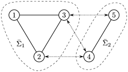
Figure 9: The multi-robot system with two clusters $\bar{\Sigma}_{1}=\{\Sigma_{1},\Sigma_{2},\Sigma_{3}\}$ and $\bar{\Sigma}_{2}=\{\Sigma_{4},\Sigma_{5}\}$. The solid lines indicate the communication links between agents and the dotted lines indicate the dynamical couplings between clusters.

The robots are subject to the following STL tasks:

$$\phi_{1} :=F_{[0,40]}G_{[0,20]}((\|\boldsymbol{p}_{1}-\boldsymbol{p}_{2}\|\leq 1)\wedge(\|\boldsymbol{p}_{1}-\boldsymbol{p}_{3}\|\leq 1)$$

$$\phi_{2} :=F_{[0,40]}G_{[0,20]}((\|\boldsymbol{p}_{2}-\boldsymbol{p}_{3}\|\leq 1)$$

$$\qquad\qquad\qquad\qquad\qquad\qquad\wedge(|\deg(x_{2,3})-\deg(x_{3,3})|\leq 7.5)$$

$$\phi_{3} :=F_{[0,40]}G_{[0,20]}((\|\boldsymbol{p}_{3}-[14;7]\|\leq 0.1)\wedge(|\deg(x_{3,3})|\leq 7.5)$$

$$\phi_{4} :=F_{[0,40]}G_{[0,20]}((\|\boldsymbol{p}_{4}-[14;7.5]\|\leq 0.1)\wedge(|\deg(x_{4,3})|\leq 7.5)$$

$$\phi_{5} :=F_{[0,40]}G_{[0,20]}((\|\boldsymbol{p}_{5}-\boldsymbol{p}_{4}\|\leq 1)$$

where $\deg(\cdot)$ converts angle units from radians to degrees. Intuitively, robots 3 and 4 are assigned to move to their predefined goal points $[14;7]$ and $[14;7.5]$, respectively, and stay there within the desired time interval, in the meanwhile satisfying the additional requirements on the robots’ orientation; robot 2 is required to chase and follow robot 3 within the desired time interval, in the meanwhile keeping a similar orientation as robot 3; robot 2 is required to chase and follow robots 2 and 3 within the desired time interval; and robot 5 is required to chase and follow robot 4. Induced by the task dependency graph, we obtain two clusters from the multi-agent system: $\bar{\Sigma}_{1}=\{\Sigma_{1},\Sigma_{2},\Sigma_{3}\}$ and $\bar{\Sigma}_{2}=\{\Sigma_{4},\Sigma_{5}\}$, as depicted in Fig. 9. Note that in Fig. 9, the solid lines indicate the communication links between agents, and the dotted lines indicate the dynamical couplings between clusters induced by the interconnection graph. Thus, the cluster interconnection graph is cyclic due to the dynamical couplings between the agents in different clusters.

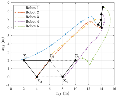
Figure 10: State trajectories of the closed-loop robot systems on the position plane. The triangles indicate the orientation of each robot. The initial states of the robots are, respectively, $\boldsymbol{x}_{1}(0)=[2;2;-\pi/4]$, $\boldsymbol{x}_{2}(0)=[4;0;0]$, $\boldsymbol{x}_{3}(0)=[6;2;\pi/4]$, $\boldsymbol{x}_{4}(0)=[8;0;0]$, $\boldsymbol{x}_{5}(0)=[10;2;-\pi/4]$. The goal positions of $\Sigma_{3}$ and $\Sigma_{4}$ are, respectively, $[14;7]$ and $[14;7.5]$.

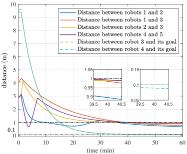
Figure 11: The evolution of the relative distances between the agents (or between an agent and its goal position) as time progresses.

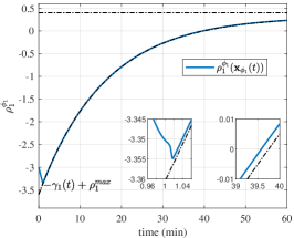
(a) Funnel for $\Sigma_{1}$ with task $\phi_{1}$

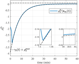
(b) Funnel for $\Sigma_{2}$ with task $\phi_{2}$

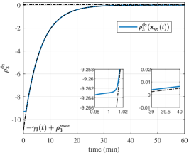
(c) Funnel for $\Sigma_{3}$ with task $\phi_{3}$

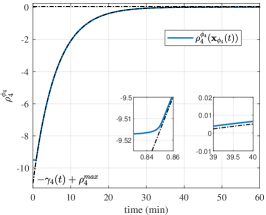
(d) Funnel for $\Sigma_{4}$ with task $\phi_{4}$

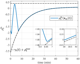
(e) Funnel for $\Sigma_{5}$ with task $\phi_{5}$

Figure 12: The funnels for the STL tasks. Performance bounds are indicated by dashed lines. Evolution of $\rho_{i}^{\phi_{i}}(\boldsymbol{x}_{\phi_{i}}(t))$ are depicted using solid lines.

To enforce the STL tasks on this 5-robot system, we apply the proposed compositional framework by leveraging the results in Theorem III.8 and applying the proposed feedback controllers as in (9). Note that Assumptions IV.1-IV.3 on the STL formulae and the system dynamics are satisfied, and the task dependency graph also satisfies Assumption IV.4. We can thus apply the feedback controller as in (9) on the agents to enforce the STL tasks in a distributed manner. Numerical implementations were performed using MATLAB on a computer with a processor Intel Core i7 3.6 GHz CPU. Note that the computation of local controllers took on average 0.1 ms, which is negligible since $\boldsymbol{u}_{i}$ is given by a closed-form expression and computed in a distributed manner. Simulation results are shown in Figs. 10-12. The state trajectories of each robot are depicted as in Fig. 10 on the position plane. The triangles are used to indicate the dynamical evolution of the orientation of each robot. The initial positions and final positions of the agents are represented by solid circles, the solid lines between the circles indicate communication links, and the dotted lines between the circles indicate dynamical couplings between the agents. In Fig. 11, we show the evolution of the relative distances between the agents (or between an agent and its goal position) as time progresses. As it can be seen from Figs. 10 and 11, all the agents satisfy their desired STL tasks. In particular, agents 3 and 4 finally achieved their tasks to reach and stay around their goal point within a certain distance (0.1 meter) after 40 minutes; agents 1, 2, and 5 achieved their tasks to chase and stay close to their desired agents within a certain distance (1 meter). In Fig. 12, we further present the temporal behaviors of $\rho_{i}^{\phi_{i}}(\mathbf{x}_{\phi_{i}}(t))$ for the 5 robots. It can be readily seen that the prescribed performances of $\rho_{i}^{\phi_{i}}(\mathbf{x}_{\phi_{i}}(t))$ are satisfied with respect to the error funnels, which verifies that the time bounds are also respected. We can conclude that all STL tasks are satisfied within the desired time interval.

VI Conclusions

We proposed a compositional approach for the synthesis of signal temporal logic tasks for large-scale multi-agent systems using assume-guarantee contracts. Each agent in the multi-agent system is subject to collaborative tasks in the sense that it does not only depend on the agent itself but may also depend on other agents. The STL tasks are first translated to assume-guarantee contracts so that the satisfaction of a contract guarantees the satisfaction of the signal temporal logic task. Two concepts of contract satisfaction were introduced to establish our compositionality results, where weak satisfaction was shown to be sufficient to deal with acyclic interconnections, and strong satisfaction was needed for cyclic interconnections. We then derived a continuous-time closed-form feedback controller to enforce the uniform strong satisfaction of local contracts in a distributed manner, thus guaranteeing the satisfaction of global STL task for the multi-agent system based on the proposed compositionality result. Finally, the theoretical results were validated via two numerical case studies.

Definition .1

(Satisfaction of assume-guarantee contracts by the clusters) Consider a cluster of agents $\bar{\Sigma}_{k}$ an assume-guarantee contract $\bar{\mathcal{C}}_{k}\!=\!(\bar{A}_{k}^{a},\bar{G}_{k})$ as in Definition III.5.

We say that $\bar{\Sigma}_{k}$ (weakly) satisfies $\bar{\mathcal{C}}_{k}$, denoted by $\bar{\Sigma}_{k}\models\bar{\mathcal{C}}_{k}$, if for any trajectory $(\bar{\mathbf{x}}_{k},\bar{\mathbf{w}}_{k})\!:\!\mathbb{R}_{\geq 0}\!\rightarrow\!\bar{X}_{k}\!\times\!\bar{W}_{k}$ of $\bar{\Sigma}_{k}$, the following holds: for all $t\in\mathbb{R}_{\geq 0}$ such that $\bar{\mathbf{w}}_{k}(s)\!\in\!\bar{A}_{k}^{a}(s)$ for all $s\in[0,t]$, we have $\bar{\mathbf{x}}_{k}(s)\in\bar{G}_{k}(s)$ for all $s\in[0,t]$.

We say that $\bar{\Sigma}_{k}$ uniformly strongly satisfies $\bar{\mathcal{C}}_{k}$, denoted by $\bar{\Sigma}_{k}\models_{us}\bar{\mathcal{C}}_{k}$, if for any trajectory $(\bar{\mathbf{x}}_{k},\bar{\mathbf{w}}_{k})\!:\!\mathbb{R}_{\geq 0}\!\rightarrow\!\bar{X}_{k}\!\times\!\bar{W}_{k}$ of $\bar{\Sigma}_{k}$, the following holds: there exists $\bar{\delta}_{k}>0$ such that for all $t\in\mathbb{R}_{\geq 0}$, $\bar{\mathbf{w}}_{k}(s)\!\in\!\bar{A}_{k}^{a}(s)$ for all $s\in[0,t]$, we have $\bar{\mathbf{x}}_{k}(s)\in\bar{G}_{k}(s)$ for all $s\in[0,t+\bar{\delta}_{k}]$.

-A Supplementaries on funnel-based control

In order to design feedback controllers to prescribe the transient behavior of $\rho_{i}^{\psi_{i}}(\mathbf{x}_{\phi_{i}}(t))$ within the predefined region:

$$-\gamma_{i}(t)<\rho_{i}^{\psi_{i}}(\mathbf{x}_{\phi_{i}}(t))-\rho_{i}^{max}<0,$$ (17)

one can translate the funnel functions into notions of errors as follows. First, define a one-dimensional error as $e_{i}(\mathbf{x}_{\phi_{i}}(t))=\rho_{i}^{\psi_{i}}(\mathbf{x}_{\phi_{i}}(t))-\rho_{i}^{max}$. Now, by normalizing the error $e_{i}(\mathbf{x}_{\phi_{i}}(t))$ with respect to the funnel function $\gamma_{i}$, we define the modulated error as

$$\hat{e}_{i}(\mathbf{x}_{\phi_{i}},t)=\frac{e_{i}(\mathbf{x}_{\phi_{i}}(t))}{\gamma_{i}(t)}.$$

Then, (17) can be rewritten as $-1<\hat{e}_{i}(t)<0$. We use $\hat{\mathcal{D}_{i}}:=(-1,0)$ to denote the performance region for $\hat{e}_{i}(t)$. Next, the modulated error is transformed through a transformation function $T_{i}:(-1,0)\rightarrow\mathbb{R}$ defined as

$$T_{i}(\hat{e}_{i}(\mathbf{x}_{\phi_{i}},t))=\ln(-\frac{\hat{e}_{i}(\mathbf{x}_{\phi_{i}},t)+1}{\hat{e}_{i}(\mathbf{x}_{\phi_{i}},t)}).$$

Note that the transformation function $T_{i}:(-1,0)\rightarrow\mathbb{R}$ is a strictly increasing function, bijective and hence admitting an inverse. By differentiating the transformed error $\epsilon_{i}:=T_{i}(\hat{e}_{i}(\mathbf{x}_{\phi_{i}},t))$ w.r.t time, we obtain

$$\dot{\epsilon}_{i}=\mathcal{J}_{i}(\hat{e}_{i},t)[\dot{e}_{i}+\alpha_{i}(t)e_{i}],$$ (18)

where $\mathcal{J}_{i}(\hat{e}_{i},t)\!=\!\frac{\partial{T_{i}(\hat{e}_{i})}}{\partial{\hat{e}_{i}}}\frac{1}{\gamma_{i}(t)}\!=\!-\frac{1}{\gamma_{i}(t)\hat{e}_{i}(1+\hat{e}_{i})}\!>\!0$, for all $\hat{e}_{i}\!\in\!(-1,0)$, is the normalized Jacobian of the transformation function, and $\alpha_{i}(t)\!=\!-\frac{\dot{\gamma}_{i}(t)}{\gamma_{i}(t)}\!>\!0$ for all $t\!\in\!\mathbb{R}_{\geq 0}$ is the normalized derivative of the performance function $\gamma_{i}$.

It can be seen that, if the transformed error $\epsilon_{i}$ is bounded for all $t$, then the modulated error $\hat{e}_{i}$ is constrained within the performance region $\hat{\mathcal{D}_{i}}$, which further implies that the error $e_{i}$ evolves within the prescribed funnel bounds as in (17).

-B Proofs not contained in the main body

Proof of Proposition III.6. We only provide the proof for the case of strong satisfaction of contracts. The case of weak satisfaction can be derived similarly.

Suppose that $\Sigma_{i}\models_{us}\mathcal{C}_{i}$ holds for all $i\in I_{k}$. Consider an arbitrary trajectory $(\bar{\mathbf{x}}_{k},\bar{\mathbf{w}}_{k})\!:\!\mathbb{R}_{\geq 0}\!\rightarrow\!\bar{X}_{k}\!\times\!\bar{W}_{k}$ of the cluster $\bar{\Sigma}_{k}$. Let us show the existence of $\bar{\delta}_{k}>0$ such that for all $t\in\mathbb{R}_{\geq 0}$ with $\bar{\mathbf{w}}_{k}(s)\in\bar{A}_{k}^{a}(s)$ for all $s\in[0,t]$, we have $\bar{\mathbf{x}}_{k}(s)\in\bar{G}_{k}(s)$ for all $s\in[0,t+\bar{\delta}_{k}]$.

First, given the trajectory $(\bar{\mathbf{x}}_{k},\bar{\mathbf{w}}_{k})\!:\!\mathbb{R}_{\geq 0}\!\rightarrow\!\bar{X}_{k}\!\times\!\bar{W}_{k}$, we have by Definition III.2 that $\bar{\mathbf{x}}_{k}=[\mathbf{x}_{k_{1}};\dots;\mathbf{x}_{k_{|I_{k}|}}]$ and $\bar{\mathbf{w}}_{k}=[\mathbf{w}_{k_{1}};\dots;\mathbf{w}_{k_{|I_{k}|}}]$, and thus, $(\mathbf{x}_{i},\mathbf{w}_{i}):\mathbb{R}_{\geq 0}\rightarrow X_{i}\times W_{i}$ is a trajectory of $\Sigma_{i}$ for all $i\in I_{k}$, where $\mathbf{w}_{i}(t)=[\mathbf{x}_{j_{1}}(t);\dots;\mathbf{x}_{j_{|\mathcal{N}_{i}^{a}|}}(t)]$. Now, consider any arbitrary $t\in\mathbb{R}_{\geq 0}$, such that $\bar{\mathbf{w}}_{k}(s)\in\bar{A}_{k}^{a}(s)$ for all $s\in[0,t]$, it follows that $\mathbf{w}_{i}(s)\in A_{i}^{a}$ for all $s\in[0,t]$ for all $i\in I_{k}$ since $\bar{A}_{k}^{a}=\prod_{i\in I_{k}}A_{i}^{a}$. Using the fact that $\Sigma_{i}\models_{us}\mathcal{C}_{i}$ for all $i\in I_{k}$, we have by Definition III.4 that for each $i\in I_{k}$ there exists $\delta_{i}$ such that $(\mathbf{x}_{i}(s),\mathbf{z}_{i}(s))\in G_{i}(s)$ for all $s\in[0,t+\delta_{i}]$, where $\mathbf{z}_{i}(t)=[\mathbf{x}_{j_{1}}(t);\dots;\mathbf{x}_{j_{|I_{k}-1|}}(t)]$ is the cooperative internal input (the stacked state of its cooperative agents that are involved in the same cluster). Let us define $\bar{\delta}_{k}=\min_{i\in I_{k}}\delta_{i}$. Then, using the fact that $\bar{G}_{k}=\cap_{i\in I_{k}}G_{i}$ we get that $\bar{\mathbf{x}}_{k}(s)=[\mathbf{x}_{k_{1}}(s);\dots;\mathbf{x}_{k_{|I_{k}|}}(s)]\in\bar{G}_{k}(s)$ for all $s\in[0,t+\bar{\delta}_{k}]$, where $G_{i}(s)\subseteq\bar{X}_{k}=X_{k_{1}}\times\ldots\times X_{i}\times\ldots\times X_{I_{k}}$. Therefore, we obtain that $\bar{\Sigma}_{k}\models_{us}\bar{\mathcal{C}}_{k}$. $\hfill\blacksquare$

Proof of Theorem III.7. Let $\mathbf{x}\!:\!\mathbb{R}_{\geq 0}\!\rightarrow\!X$ be a trajectory of the multi-agent system $\Sigma$. Then, from the definition of multi-agent systems, we have for all $i\in I$, $(\mathbf{x}_{i},\mathbf{w}_{i}):\mathbb{R}_{\geq 0}\rightarrow X_{i}\times W_{i}$ is a trajectory of $\Sigma_{i}$, where $\mathbf{x}=[\mathbf{x}_{1};\dots;\mathbf{x}_{N}]$, and $\mathbf{w}_{i}(t)=[\mathbf{x}_{j_{1}}(t);\dots;\mathbf{x}_{j_{|\mathcal{N}_{i}^{a}|}}(t)]$.

Since the cluster interconnection graph $\bar{\mathcal{G}}^{a}=(\bar{I},\bar{E}^{a})$ is a directed acyclic graph, there exists at least one initial cluster that does not have adversarial internal inputs. Now, consider the initial clusters $\{\bar{\Sigma}_{k}\}_{k\in\bar{I}^{Init}}$. First, we have by condition (i) that $\Sigma_{i}\models\mathcal{C}_{i}$ holds for all $i\in I$, and thus we obtain that $\bar{\Sigma}_{k}\models\bar{\mathcal{C}}_{k}$ by Proposition III.6. This implies that for all $t\in\mathbb{R}_{\geq 0}$ with $\bar{\mathbf{w}}_{k}(s)\in\bar{A}_{k}^{a}(s)$ for all $s\in[0,t]$, we have $\bar{\mathbf{x}}_{k}(s)\in\bar{G}_{k}(s)$ for all $s\in[0,t]$. Now consider a $t\in\mathbb{R}_{\geq 0}$ and assume that $\bar{\mathbf{w}}_{k}(s)\in\bar{A}_{k}^{a}(s)$ for all $s\in[0,t]$. Since the initial clusters do not have adversarial internal inputs, this implies that:

$$\bar{\mathbf{x}}_{k}(s)\in\bar{G}_{k}(s),\forall s\in[0,t],\forall k\in\bar{I}^{Init}.$$ (19)

Next, let us prove by contradiction that for all $k\in\bar{I}$, $\bar{\mathbf{x}}_{k}(s)\in\bar{G}_{k}(s)$, for all $s\in[0,t]$. Let us assume that there exists $k\in\bar{I}\setminus\bar{I}^{Init}$, such that $\bar{\mathbf{x}}_{k}(s)\notin\bar{G}_{k}(s)$, for some $s\in[0,t]$. Since by condition (i) we have $\Sigma_{i}\models\mathcal{C}_{i}$ for all $i\in I$, which implies that $\bar{\Sigma}_{k}\models\bar{\mathcal{C}}_{k}$ by Proposition III.6, we have that $\bar{\mathbf{w}}_{k}(s)\notin\bar{A}_{k}^{a}(s)$ for some $s\in[0,t]$. Since $\bar{\mathbf{w}}_{k}=[\mathbf{w}_{k_{1}};\dots;\mathbf{w}_{k_{|I_{k}|}}]$, this means that for some $i\in I_{k}$, $\mathbf{w}_{i}(s)\notin A_{i}^{a}(s)$. Then using the fact that: $\mathbf{w}_{i}(s)=[\mathbf{x}_{j_{1}}(s);\dots;\mathbf{x}_{j_{|\mathcal{N}_{i}^{a}|}}(s)]$ and $\prod_{j\in\mathcal{N}_{i}^{a}}\overline{\textbf{Proj}}^{j}(G_{j}(s)\subseteq A_{i}^{a}(s)$, we deduce the existence of $j\in\mathcal{N}_{i}^{a}$ such that $\mathbf{x}_{j}(s)\notin\overline{\textbf{Proj}}^{j}(G_{j}(s))$, which further implies that $\bar{\mathbf{x}}_{k^{\prime}}(s)\notin\bar{G}_{k^{\prime}}(s)$, for some $s\in[0,t]$ where $j\in I_{k^{\prime}}$. By using the structure of a DAG, and by iterating this argument, there exists $l\in\bar{I}^{Init}$ such that $\bar{\mathbf{x}}_{l}(s)\notin\bar{G}_{l}(s)$, which contradicts (19). Hence, we have for all $k\in\bar{I}$, $\bar{\mathbf{x}}_{k}(s)\in\bar{G}_{k}(s)$, for all $s\in[0,t]$, and thus, $\mathbf{x}(s)=[\bar{\mathbf{x}}_{1}(s);\ldots;\bar{\mathbf{x}}_{K}(s)]\in\prod_{k\in\bar{I}}\bar{G}_{k}(s)=G(s)$ for all $s\in[0,t]$. Therefore, $\Sigma\models\mathcal{C}$. $\hfill\blacksquare$

Proof of Theorem III.8. Let $\mathbf{x}\!:\!\mathbb{R}_{\geq 0}\!\rightarrow\!X$ be a trajectory of the multi-agent system $\Sigma$. Then, from the definition of multi-agent systems, we have for all $i\in I$, $(\mathbf{x}_{i},\mathbf{w}_{i}):\mathbb{R}_{\geq 0}\rightarrow X_{i}\times W_{i}$ is a trajectory of $\Sigma_{i}$, where $\mathbf{x}=[\mathbf{x}_{1};\dots;\mathbf{x}_{N}]$, and $\mathbf{w}_{i}(t)=[\mathbf{x}_{j_{1}}(t);\dots;\mathbf{x}_{j_{|\mathcal{N}_{i}^{a}|}}(t)]$.

We prove $\Sigma\models\mathcal{C}$ by showing the existence of $\delta>0$ such that $\mathbf{x}(s)\in G(s)$ for all $s\in[n\delta,(n+1)\delta)]$ for all $n\in\mathbb{N}$. First, we have from (i) that for all $i\in I$, $\mathbf{w}_{i}(0)\!=\![\mathbf{x}_{j_{1}}(0);\dots;\mathbf{x}_{j_{|\mathcal{N}_{i}^{a}|}}(0)]\in\prod_{j\in\mathcal{N}_{i}^{a}}\overline{\textbf{Proj}}^{j}(G_{j}(0))\subseteq A_{i}^{a}(0)$, where the set inclusion follows from (iii). Now, consider the clusters $\bar{\Sigma}_{k}$, $k\in\bar{I}$, in the multi-agent system. We have from (ii) that $\Sigma_{i}\models_{us}\mathcal{C}_{i}$ holds for all $i\in I$, and thus $\bar{\Sigma}_{k}\models_{us}\bar{\mathcal{C}}_{k}$ for all $k\in\bar{I}$ by Proposition III.6. Note that by the definition of clusters, we have $\bar{\mathbf{w}}_{k}(0)=[\mathbf{w}_{k_{1}}(0);\dots;\mathbf{w}_{k_{|I_{k}|}}(0)]\in\bar{A}_{k}^{a}(0)=\prod_{i\in I_{k}}A_{i}^{a}(0)$, since $\mathbf{w}_{i}(0)\in A_{i}^{a}(0)$ holds for all $i\in I$. Given that $\bar{\Sigma}_{k}\models_{us}\bar{\mathcal{C}}_{k}$, we thus have the existence of $\bar{\delta}_{k}>0$ such that for $\bar{\mathbf{w}}_{k}(0)\in\bar{A}_{k}^{a}(0)$, we have $\bar{\mathbf{x}}_{k}(s)=[\mathbf{x}_{k_{1}}(s);\dots;\mathbf{x}_{k_{|I_{k}|}}(s)]\in\bar{G}_{k}(s)$ for all $s\in[0,\bar{\delta}_{k}]$. Let us define $\delta>0$ as $\delta\!:=\!\min_{k\in\bar{I}}\bar{\delta}_{k}$. Then, it follows that $\mathbf{x}(s)=[\bar{\mathbf{x}}_{1}(s);\ldots;\bar{\mathbf{x}}_{K}(s)]\in\prod_{k\in\bar{I}}\bar{G}_{k}(s)=G(s)$ for all $s\in[0,\delta]$.

Next, let us show by induction that $\mathbf{x}(s)\in G(s)$ for all $s\in[n\delta,(n+1)\delta)]$. First, let us assume that $\mathbf{x}(s)\in G(s)$ for all $s\in[n\delta,(n+1)\delta)]$ and show that $\mathbf{x}(s)\in G(s)$ for all $s\!\in\![(n+1)\delta,(n+2)\delta)]$. By $\mathbf{x}(s)\in G(s)$ for all $s\in[n\delta,(n+1)\delta)]$, we obtain that $\bar{\mathbf{x}}_{k}(s)\in\bar{G}_{k}(s)$ for all $s\in[n\delta,(n+1)\delta)]$ for all $k\in\bar{I}$, since $\mathbf{x}(s)=[\bar{\mathbf{x}}_{1}(s);\ldots;\bar{\mathbf{x}}_{K}(s)]\in G(s)=\prod_{k\in\bar{I}}\bar{G}_{k}(s)$. This further implies that $(\mathbf{x}_{i}(s),\mathbf{z}_{i}(s))\in G_{i}(s)$ for all $s\in[n\delta,(n+1)\delta)]$ for all $i\in I$, since $\bar{\mathbf{x}}_{k}(s)=[\mathbf{x}_{k_{1}}(s);\dots;\mathbf{x}_{k_{|I_{k}|}}(s)]\in\bar{G}_{k}(s)=\cap_{i\in I_{k}}G_{i}(s)$, where $G_{i}(s)\subseteq\bar{X}_{k}=X_{k_{1}}\times\ldots\times X_{i}\times\ldots\times X_{I_{k}}$. Then, we obtain that for all $i\in I_{k}$, and for all $s\in[n\delta,(n+1)\delta]$, $\mathbf{w}_{i}(s)\!=\!$ $[\mathbf{x}_{j_{1}}(s);\dots;\mathbf{x}_{j_{|\mathcal{N}_{i}|}}(s)]\in\prod_{j\in\mathcal{N}_{i}^{a}}\overline{\textbf{Proj}}^{j}(G_{j}(s))\subseteq A_{i}^{a}(s)$, where the set inclusion follows from (iii). This implies that $\bar{\mathbf{w}}_{k}(s)=[\mathbf{w}_{k_{1}}(s);\dots;\mathbf{w}_{k_{|I_{k}|}}(s)]\in\prod_{i\in I_{k}}A_{i}^{a}(s)=\bar{A}_{k}^{a}(s)$ for all $s\in[n\delta,(n+1)\delta]$. Again, since $\bar{\Sigma}_{k}\models_{us}\bar{\mathcal{C}}_{k}$, one gets for all $k\in\bar{I}$, $\bar{\mathbf{x}}_{k}(s)=[\mathbf{x}_{k_{1}}(s);\dots;\mathbf{x}_{k_{|I_{k}|}}(s)]\in\bar{G}_{k}(s)$ for all $s\in[(n+1)\delta,(n+1)\delta+\bar{\delta}_{k}]$, which further implies that $\bar{\mathbf{x}}_{k}(s)\in\bar{G}_{k}(s)$ for all $s\in[(n+1)\delta,(n+2)\delta]$ since $\delta\!:=\!\min_{k\in\bar{I}}\bar{\delta}_{k}$. Hence, $\mathbf{x}(s)=[\bar{\mathbf{x}}_{1}(s);\ldots;\bar{\mathbf{x}}_{K}(s)]\in\prod_{k\in\bar{I}}\bar{G}_{k}(s)=G(s)$ for all $s\in[(n+1)\delta,(n+2)\delta)]$. Therefore, by induction, one has that $\mathbf{x}(s)\in G(s)$ for all $s\in[n\delta,(n+1)\delta)]$ for all $n\in\mathbb{N}$, and thus for all $s\geq 0$, which concludes that $\Sigma\models\mathcal{C}$. $\hfill\blacksquare$

Proof of Proposition III.11. Consider $\varepsilon>0$ such that $\Sigma_{i}\models\mathcal{C}_{i}^{\varepsilon}$. From uniform continuity of $\mathbf{w}_{i}:\mathbb{R}_{\geq 0}\rightarrow W_{i}$, and for $\varepsilon>0$, we have the existence of $\delta_{i}>0$ such that for all $t\geq 0$, if $\mathbf{w}_{i}(s)\in A_{i}^{a}(s)$, for all $s\in[0,t]$, then $\mathbf{w}_{i}(s)\in\mathcal{B}_{\varepsilon}(A_{i}^{a})(s)$, for all $s\in[0,t+\delta_{i}]$.

Let us now show the uniform strong satisfaction of contracts. Consider the $\delta_{i}>0$ defined above, and consider any $t\geq 0$ such that $\mathbf{w}_{i}(s)\in A_{i}^{a}(s)$ for all $s\in[0,t]$. First we have by the uniform continuity of $\mathbf{w}_{i}$, $\mathbf{w}_{i}(s)\in\mathcal{B}_{\varepsilon}(A_{i}^{a})(s)$, for all $s\in[0,t+\delta_{i}]$. Hence, from the weak satisfaction of $\mathcal{C}_{i}^{\varepsilon}$, one has that $(\mathbf{x}_{i}(s),\mathbf{z}_{i}(s))\in G_{i}(s)$ for all $s\in[0,t+\delta_{i}]$, which in turn implies the uniform strong satisfaction of the contract $\mathcal{C}_{i}$.

Hence, $\Sigma_{i}\models_{us}\mathcal{C}_{i}$. $\hfill\blacksquare$

Proof of Theorem IV.5. We prove the uniform strong satisfaction of the contract using Proposition III.11. Let $(\mathbf{x}_{i},\mathbf{w}_{i}):\mathbb{R}_{\geq 0}\rightarrow X_{i}\times W_{i}$ be a trajectory of $\Sigma_{i}$. Since $-\gamma_{i}(0)+\rho_{i}^{max}<\rho_{i}^{\psi_{i}}(\mathbf{x}_{i}(0))<\rho_{i}^{max}$ holds, we have $\mathbf{x}_{i}(0)\in G_{i}$. Now, consider $\varepsilon>0$. Let us prove $\Sigma_{i}\models\mathcal{C}_{i}^{\varepsilon}$, where $\mathcal{C}_{i}^{\varepsilon}=(\mathcal{B}_{\varepsilon}(A_{i}^{a}),G_{i})$. Let $s\in\mathbb{R}_{\geq 0}$, such that for all $t\in[0,s]$, $\mathbf{w}_{i}(t)\in\mathcal{B}_{\varepsilon}(A_{i}^{a})$, i.e., for all $j\in\mathcal{N}_{i}$, $-\gamma_{j}(t)+\rho_{j}^{max}-\varepsilon<\rho_{j}^{\psi_{j}}(\mathbf{x}_{j}(t))<\rho_{j}^{max}+\varepsilon$ holds for all $t\in[0,s]$. Next, we show that ${\mathbf{x}_{i}}_{|[0,s]}\in G_{i}$.

Consider the cluster of agents $\bar{\Sigma}_{k}$ with $i\in I_{k}$ where each agent is subject to STL task $\phi_{i}$. Let us define $\epsilon=[\epsilon_{1};\ldots;\epsilon_{|I_{k}|}]$. Consider a Lyapunov-like function $V:\mathbb{R}^{|I_{k}|}\rightarrow\mathbb{R}_{\geq 0}$ defined as $V(\epsilon)=\frac{1}{2}\epsilon^{\top}\epsilon$.

By differentiating $V$ with respect to time, we obtain $\dot{V}=\epsilon^{\top}\dot{\epsilon}$, where each $\dot{\epsilon}_{i}$ can be obtained by

$$\dot{\epsilon}_{i}\stackrel{{\scriptstyle\eqref{transerror_dynamics}}}{{=}} \mathcal{J}_{i}(\hat{e}_{i},t)[\dot{e}_{i}+\alpha_{i}(t)e_{i}]$$

$$= \mathcal{J}_{i}(\hat{e}_{i},t)[\frac{\partial{\rho_{i}^{\psi_{i}}(\mathbf{x}_{i})}}{\partial\mathbf{x}_{i}}^{\top}\mathbf{\dot{x}}_{i}(t)-\dot{\gamma}_{i}(t)\hat{e}_{i}].$$

Thus, $\dot{V}$ can be obtained as

$$\dot{V}=\epsilon^{\top}\dot{\epsilon}=\epsilon^{\top}\mathcal{J}(\Gamma\dot{\bar{\mathbf{x}}}_{k}-\mathbf{p}),$$ (20)

where $\mathcal{J}\in\mathbb{R}^{|I_{k}|\times|I_{k}|}$ is a diagonal matrix with diagonal entries $\mathcal{J}_{i}(\hat{e}_{i})\!=\!-\frac{1}{\gamma_{i}(t)\hat{e}_{i}(1+\hat{e}_{i})}$, $i\in I_{k}$, $\Gamma\in\mathbb{R}^{|I_{k}|\times\bar{n}_{k}}$ is a matrix with row vectors $\frac{\partial{\rho_{i}^{\psi_{i}}(\mathbf{x}_{\phi_{i}})}}{\partial\bar{\mathbf{x}}_{k}}^{\top}$, and $\mathbf{p}\in\mathbb{R}^{|I_{k}|}$ is a column vector with entries $\dot{\gamma}_{i}(t)\hat{e}_{i}$. By inserting the dynamics of $\dot{\bar{\mathbf{x}}}_{k}$ (5) into (20), we obtain that

$$\dot{V}= \epsilon^{\top}\mathcal{J}(\Gamma(\bar{f}_{k}(\bar{\mathbf{x}}_{k})+\bar{g}_{k}(\bar{\mathbf{x}}_{k})\bar{\mathbf{u}}_{k}+\bar{h}_{k}(\bar{\mathbf{w}}_{k}))-\mathbf{p})$$

$$= \epsilon^{\top}\mathcal{J}(\Gamma(\bar{f}_{k}(\bar{\mathbf{x}}_{k})+\bar{h}_{k}(\bar{\mathbf{w}}_{k}))-\mathbf{p})+\epsilon^{\top}\mathcal{J}\Gamma\bar{g}_{k}(\bar{\mathbf{x}}_{k})\bar{\mathbf{u}}_{k},$$ (21)

where $\bar{\mathbf{u}}_{k}\!=[\mathbf{u}_{k_{1}};\dots;\mathbf{u}_{k_{|I_{k}|}}]$, with the local control law $\mathbf{u}_{i}=-g_{i}^{\top}(\mathbf{x}_{i})\sum_{j\in I_{k}}(\frac{\partial\rho_{j}^{\psi_{j}}({\mathbf{x}}_{\phi_{j}})}{\partial\mathbf{x}_{i}}\mathcal{J}_{j}(\hat{e}_{j},t)\epsilon_{j}({\mathbf{x}}_{\phi_{j}},t))$ as in (9), $i\in I_{k}=\{{k_{1}},\ldots,{k_{|I_{k}|}}\}$. Then, we get

$$\dot{V}= \epsilon^{\top}\mathcal{J}(\Gamma(\bar{f}_{k}(\bar{\mathbf{x}}_{k})+\bar{h}_{k}(\bar{\mathbf{w}}_{k})-\Theta\mathbf{d})-\mathbf{p})$$ (22)

$$-\epsilon^{\top}\mathcal{J}\Gamma\Theta\Lambda\mathcal{J}\epsilon,$$

where $\Theta:=\textup{diag}(g_{k_{i}}(\mathbf{x}_{k_{i}})g_{k_{i}}^{\top}(\mathbf{x}_{k_{i}}))\in\mathbb{R}^{\bar{n}_{k}\times\bar{n}_{k}}$, $\mathbf{d}\in\mathbb{R}^{\bar{n}_{k}}$ is a column vector with entries $h_{i}(d_{i})$, and $\Lambda\in\mathbb{R}^{\bar{n}_{k}\times|I_{k}|}$ is a matrix with column vectors $\frac{\partial{\rho_{i}^{\psi_{i}}(\mathbf{x}_{\phi_{i}})}}{\partial\bar{\mathbf{x}}_{k}}=[\frac{\partial{\rho_{i}^{\psi_{i}}(\mathbf{x}_{\phi_{i}})}}{\partial{\mathbf{x}}_{i_{1}}};\ldots;\frac{\partial{\rho_{i}^{\psi_{i}}(\mathbf{x}_{\phi_{i}})}}{\partial{\mathbf{x}}_{i_{|P_{i}|}}}]$. Recall that $\Gamma\in\mathbb{R}^{|I_{k}|\times\bar{n}_{k}}$ is a matrix with row vectors $\frac{\partial{\rho_{i}^{\psi_{i}}(\mathbf{x}_{\phi_{i}})}}{\partial\bar{\mathbf{x}}_{k}}^{\top}$, we get that $\Gamma=\Lambda^{\top}$. Then by (22), and thus $-\epsilon^{\top}\mathcal{J}\Gamma\Theta\Lambda\mathcal{J}\epsilon=-\epsilon^{\top}\mathcal{J}\Lambda^{\top}\Theta\Lambda\mathcal{J}\epsilon$. Note that by Assumption IV.4, we get that $\Lambda$ is a block matrix that can be converted to an upper triangular form. Moreover, the diagonal entries of the block matrix $\Lambda$ are non-zero since $\frac{\partial\rho_{i}^{\psi_{i}}({\mathbf{x}}_{\phi_{i}})}{\partial\mathbf{x}_{i}}$ are non-zero. Therefore, we can obtain that the rank of matrix $\Lambda$ is $\text{rank}(\Lambda)=|I_{k}|$. Note that according to Assumption IV.3, $g_{i}(\mathbf{x}_{i})g_{i}(\mathbf{x}_{i})^{\top}$ is positive definite. Therefore, the matrix $\Lambda^{\top}\Theta\Lambda$ is positive definite. Then, we can obtain that $\Lambda^{\top}\Theta\Lambda\geq\alpha_{L}I_{|I_{k}|}$ for some $\alpha_{L}>0$. Recall that $\mathcal{J}\in\mathbb{R}^{|I_{k}|\times|I_{k}|}$ is a diagonal matrix with positive diagonal entries $\mathcal{J}_{i}(\hat{e}_{i})\!=\!-\frac{1}{\gamma_{i}(t)\hat{e}_{i}(1+\hat{e}_{i})}$, thus, $\mathcal{J}^{2}\geq\alpha_{J}I_{|I_{k}|}$, where $\alpha_{J}=\min_{i\in I_{k}}\{\frac{1}{\sup_{t\in\mathbb{R}_{\geq 0}}\gamma_{i}(t)^{2}}\min_{\hat{e}_{i}\in\hat{\mathcal{D}_{i}}}(\frac{1}{\hat{e}_{i}(1+\hat{e}_{i})})^{2}\}>0$. Hence, we obtain that $-\epsilon^{\top}\mathcal{J}\Lambda^{\top}\Theta\Lambda\mathcal{J}\epsilon\leq-\alpha_{L}\alpha_{J}\epsilon^{\top}\epsilon\leq-2\alpha_{L}\alpha_{J}V$. Hence, we get the chain of inequality

$$\dot{V}= \epsilon^{\top}\mathcal{J}(\Gamma(\bar{f}_{k}(\bar{\mathbf{x}}_{k})+\bar{h}_{k}(\bar{\mathbf{w}}_{k})-\Theta\mathbf{d})-\mathbf{p})$$

$$-\epsilon^{\top}\mathcal{J}\Lambda^{\top}\Theta\Lambda\mathcal{J}\epsilon,$$

$$\leq \epsilon^{\top}\mathcal{J}(\Gamma(\bar{f}_{k}(\bar{\mathbf{x}}_{k})+\bar{h}_{k}(\bar{\mathbf{w}}_{k})-\Theta\mathbf{d})-\mathbf{p})$$

$$-\epsilon^{\top}\mathcal{J}(\alpha_{L}-\xi)\mathcal{J}\epsilon-\xi\|\epsilon^{\top}\mathcal{J}\|^{2}$$

$$\leq {{\color[rgb]{0,0,0}{\bf}-\kappa V+\eta(t)}}$$ (23)

for some $\xi$ satisfying $0<\xi<\alpha_{L}$, where $\kappa=2(\alpha_{L}-\xi)\alpha_{J}$, $\eta(t)=\frac{1}{4\xi}(\|\Gamma\|(\|\bar{f}_{k}(\bar{\mathbf{x}}_{k})\|+\|\bar{h}_{k}(\bar{\mathbf{w}}_{k})\|+\|\Theta\mathbf{d}\|)+\|\mathbf{p}\|)^{2}$.

Now, we proceed with finding an upper bound of $\eta(t)$. Since $-\gamma_{i}(0)+\rho_{i}^{max}<\rho_{i}^{\psi_{i}}(\mathbf{x}_{\phi_{i}}(0))<\rho_{i}^{max}$, $\mathbf{x}_{\phi_{i}}(0)$ is such that $\hat{e}_{i}(\mathbf{x}_{\phi_{i}}(0),0)\in\hat{\mathcal{D}_{i}}=(-1,0)$. Now, define the set $\mathcal{X}_{i}(t):=\{\mathbf{x}_{\phi_{i}}\in\mathbb{R}^{n_{P_{i}}}|-1<\hat{e}_{i}(\mathbf{x}_{\phi_{i}},t)=\frac{\rho_{i}^{\psi_{i}}(\mathbf{x}_{\phi_{i}})-\rho_{i}^{max}}{\gamma_{i}(t)}<0\}$. Note that $\mathcal{X}_{i}(t)$ has the property that for $t_{1}<t_{2}$, $\mathcal{X}_{i}(t_{2})\subseteq\mathcal{X}_{i}(t_{1})$ holds since $\gamma_{i}(t)$ is non-increasing in $t$. Also note that $\mathcal{X}_{i}(t)$ is bounded due to condition (ii) of Assumption IV.1 and $\gamma_{i}$ is bounded by definition, for all $i\in I_{k}$. According to [48, Proposition 1.4.4], the inverse image of an open set under a continuous function is open. By defining $\hat{e}_{i,0}(\mathbf{x}_{\phi_{i}}):=\hat{e}_{i}(\mathbf{x}_{\phi_{i}},0)$, we obtain that the inverse image $\hat{e}_{i,0}^{-1}(\hat{\mathcal{D}_{i}})=\mathcal{X}_{i}(0)$ is open. Since $\mathbf{x}_{\phi_{i}}\in\mathcal{X}_{i}(0)$ is bounded, we obtain that $\mathbf{x}_{i}$ for all $i\in I_{\phi_{i}}$ are evolving in a bounded region. Thus, by the continuity of functions $f_{i}$, $g_{i}$ and $h_{i}$, it holds that $\|f_{i}(\mathbf{x}_{i})\|$ and $\|g_{i}(\mathbf{x}_{i})g_{i}(\mathbf{x}_{i})^{\top}h_{i}(d_{i}(t))\|$ are upper bounded, where $d_{i}(t)=[\gamma_{j_{1}}(t)\mathbf{1}_{n_{j_{1}}};\dots;\gamma_{j_{|\mathcal{N}_{i}|}}(t)\mathbf{1}_{n_{|\mathcal{N}_{i}|}}]$. Thus, $\|\bar{f}_{k}(\bar{\mathbf{x}}_{k})\|$ and $\|\Theta\mathbf{d}\|$ are bounded. Note that $\mathbf{p}$ is a column vector with entries $\dot{\gamma}_{i}(t)\hat{e}_{i}$. Since $|\dot{\gamma}_{i}(t)\hat{e}_{i}|\leq|\dot{\gamma}_{i}(0)|$ and $|\dot{\gamma}_{i}(0)|$ is bounded by definition, $\|\mathbf{p}\|$ is bounded as well. Moreover, by combining condition (ii) of Assumption IV.1 and the assumption in the assume-guarante contract that $\mathbf{w}_{i}(t)\in\mathcal{B}_{\varepsilon}(A_{W_{i}})$, for all $t\in[0,s]$, where $\mathbf{w}_{i}=[\mathbf{x}_{j_{1}};\dots;\mathbf{x}_{j_{|\mathcal{N}_{i}|}}]$, it holds that $\|h_{i}(\mathbf{w}_{i})\|$ is also upper bounded, and thus $\|\bar{h}_{k}(\bar{\mathbf{w}}_{k})\|$ is bounded as well. Additionally, note that $\frac{\partial{\rho_{i}^{\psi_{i}}(\mathbf{x}_{\phi_{i}})}}{\partial\mathbf{x}_{\phi_{i}}}=0$ if and only if $\rho_{i}^{\psi_{i}}(\mathbf{x}_{\phi_{i}})=\rho_{i}^{opt}$ since $\rho_{i}^{\psi}(\mathbf{x}_{\phi_{i}})$ is concave under Assumption IV.1. However, since $\rho_{i}^{\psi_{i}}(\mathbf{x}_{\phi_{i}}(0))<\rho_{i}^{max}<\rho_{i}^{opt}$, and for all states $\mathbf{x}_{\phi_{i}}\in\mathcal{X}_{i}(0)$, $\rho_{i}^{\psi_{i}}(\mathbf{x}_{\phi_{i}})<\rho_{i}^{max}$ holds, then, we have for all states $\mathbf{x}_{\phi_{i}}\in\mathcal{X}_{i}(0)$, $\frac{\partial{\rho_{i}^{\psi_{i}}(\mathbf{x}_{\phi_{i}})}}{\partial\mathbf{x}_{\phi_{i}}}\neq 0_{n_{i}}$, and $\|\frac{\partial{\rho_{i}^{\psi_{i}}(\mathbf{x}_{\phi_{i}})}}{\partial\mathbf{x}_{\phi_{i}}}\|^{2}\geq k_{\rho}>0$ holds for a positive constant $k_{\rho}$. Since $\Gamma$ is a matrix with row vectors $\frac{\partial{\rho_{i}^{\psi_{i}}(\mathbf{x}_{\phi_{i}})}}{\partial\bar{\mathbf{x}}_{k}}^{\top}$, we get that $\|\Gamma\|$ is bounded. Consequently, we can define an upper bound $\bar{\eta}$ of $\eta(t)$, for all $\mathbf{x}_{\phi_{i}}\in\mathcal{X}_{i}(0)$ for all $i\in I_{k}$.

Next, define $\hat{\mathcal{D}}:=\hat{\mathcal{D}}_{1}\times\ldots\times\hat{\mathcal{D}}_{|I_{k}|}$, $i\in I_{k}$, and $\hat{e}=[\hat{e}_{1};\ldots;\hat{e}_{|I_{k}|}]$. we show that $\hat{\mathcal{D}}$ is an attraction set. To do this, we first introduce a function $\mathcal{S}(\hat{e})=1-e^{-V(\hat{e})}$ for which $0<\mathcal{S}(\hat{e})<1$, $\forall\hat{e}_{i}\in\hat{\mathcal{D}_{i}}$ , $\forall i\in I_{k}$, and $\mathcal{S}(\hat{e})\rightarrow 1$ as $\hat{e}\rightarrow\partial\hat{\mathcal{D}}$. By differentiating $\mathcal{S}(\hat{e})$ we get

$$\dot{\mathcal{S}}(t)=\dot{V}(\hat{e})\big{(}1-\mathcal{S}(\hat{e})\big{)}.$$ (24)

By substituting (23) and inserting $V(\hat{e})=-\ln{(1-\mathcal{S}(\hat{e}))}$ in (24), we get

$$\dot{\mathcal{S}}(t)\leq-\kappa\big{(}1-\mathcal{S}(\hat{e})\big{)}\big{(}\ln{(e^{-\frac{\eta(t)}{\kappa}})}-\ln{(1-\mathcal{S}(\hat{e}))}\big{)}.$$ (25)

Note that by definition, we have $\kappa>0$ and $1-\mathcal{S}(\hat{e})>0$. Now define the region $\Omega_{\hat{e}}=\{\hat{e}\in\hat{\mathcal{D}}|\mathcal{S}(\hat{e})\leq 1-e^{-\frac{\bar{\eta}}{\kappa}}\}$. Since $-\gamma_{i}(0)+\rho_{i}^{max}<\rho_{i}^{\psi_{i}}(\mathbf{x}_{\phi_{i}}(0))<\rho_{i}^{max}$ holds $\forall i\in I_{k}$, then we obtain that $\hat{e}_{i}(\mathbf{x}_{\phi_{i}}(0))\in\hat{\mathcal{D}_{i}}=(-1,0)$ $\forall i\in I_{k}$, and consequently, $\mathcal{S}(\hat{e}(0))<1$ holds. Let us define $c=\mathcal{S}(\hat{e}(0))$ and the set $\Omega_{c}=\{\hat{e}\in\hat{\mathcal{D}}|\mathcal{S}(\hat{e})\leq c\}$. Now, consider the case when $c<1-e^{-\frac{\bar{\eta}}{\kappa}}$. In this case, $\Omega_{c}\subset\Omega_{\hat{e}}$, and by (25), $\dot{\mathcal{S}}(t)\leq 0$ for all $\hat{e}\in\partial{\Omega_{\hat{e}}}$, therefore, $\hat{e}(t)\in\Omega_{\hat{e}}$, $\forall t\in\mathbb{R}_{\geq 0}$. Next, consider the other case when $c\geq 1-e^{-\frac{\bar{\eta}}{\kappa}}$. In this case $\Omega_{\hat{e}}\subseteq\Omega_{c}$, and by (25), $\dot{\mathcal{S}}(t)<0$ for all $\hat{e}\in\Omega_{c}\setminus\Omega_{\hat{e}}$, hence, $\mathcal{S}(\hat{e})\rightarrow\Omega_{\hat{e}}$. Thus, starting from any point within the set $\Omega_{c}$, $\mathcal{S}(\hat{e}(t))$ remains less than $1$. Consequently, the modulated error $\hat{e}$ always evolves within a closed strict subset of $\hat{\mathcal{D}}$ (that is, set $\Omega_{\hat{e}}$ in the case that $c<1-e^{-\frac{\bar{\eta}}{\kappa}}$, or set $\Omega_{c}$ in the case that $c\geq 1-e^{-\frac{\bar{\eta}}{\kappa}}$), which implies that $\hat{e}$ is not approaching the boundary $\partial\hat{\mathcal{D}}$. It follows that the transformed error $\epsilon$ is bounded, and thus, $\epsilon_{i}$ is bounded for all $i\in I_{k}$. Thus, we can conclude that $\rho_{i}^{\psi_{i}}(\mathbf{x}_{\phi_{i}}(t))$ evolves within the predefined region (6), i.e., ${\mathbf{x}_{\phi_{i}}}(t))\in G_{i}$ for all $t\in\mathbb{R}_{\geq 0}$. Therefore, we have $\Sigma_{i}\models\mathcal{C}_{i}^{\varepsilon}$. By Proposition III.11, it implies that $\Sigma_{i}\models_{us}\mathcal{C}_{i}$. $\hfill\blacksquare$

Part of the proof above was inspired by [49, Thm. 1], where similar Lyapunov arguments were used in the context of funnel-based control of multi-agent systems. However, the results there deal with consensus control of multi-agent systems only and cannot handle temporal logic properties.

Proof of Corollary IV.7. From Theorem IV.5, one can verify that the closed-loop agents under controller (9) satisfy: for all $i\in I$, $\Sigma_{i}\models_{us}\mathcal{C}_{i}$, and for all $i\in I$, $\prod_{j\in\mathcal{N}_{i}^{a}}\overline{\textbf{Proj}}^{j}(G_{j})\subseteq A_{i}^{a}$. Moreover, for all $i\in I$ and for any trajectory $(\mathbf{x}_{i},\mathbf{w}_{i}):\mathbb{R}_{\geq 0}\rightarrow X_{i}\times W_{i}$ of $\Sigma_{i}$, the choice of parameters of the funnel as in (10)–(15) ensures that $\mathbf{x}_{i}(0)\in\overline{\textbf{Proj}}^{i}(G_{i})(0)$. Hence, all conditions required in Theorem III.8 are satisfied, and thus, we conclude that $\Sigma\models\mathcal{C}=(\emptyset,\prod_{k\in\bar{I}}\bar{G}_{k})$ as a consequence of Theorem III.8. Therefore, the multi-agent system $\Sigma$ satisfies the STL task $\bar{\phi}=\land_{i=1}^{N}\phi_{i}$. $\hfill\blacksquare$

References

- [1] H. G. Tanner, A. Jadbabaie, and G. J. Pappas, “Stable flocking of mobile agents, part i: Fixed topology,” in 42nd IEEE International Conference on Decision and Control (IEEE Cat. No. 03CH37475), vol. 2. IEEE, 2003, pp. 2010–2015.
- [2] W. Ren and R. W. Beard, “Consensus seeking in multiagent systems under dynamically changing interaction topologies,” IEEE Transactions on automatic control, vol. 50, no. 5, pp. 655–661, 2005.
- [3] R. Olfati-Saber, J. A. Fax, and R. M. Murray, “Consensus and cooperation in networked multi-agent systems,” Proceedings of the IEEE, vol. 95, no. 1, pp. 215–233, 2007.
- [4] J. Cortes, S. Martinez, T. Karatas, and F. Bullo, “Coverage control for mobile sensing networks,” IEEE Transactions on robotics and Automation, vol. 20, no. 2, pp. 243–255, 2004.
- [5] M. Mesbahi and M. Egerstedt, Graph theoretic methods in multiagent networks. Princeton University Press, 2010.
- [6] P. Tabuada, Verification and control of hybrid systems: a symbolic approach. Springer Science & Business Media, 2009.
- [7] C. Belta, B. Yordanov, and E. A. Gol, Formal methods for discrete-time dynamical systems. Springer, 2017, vol. 15.
- [8] M. Kloetzer and C. Belta, “A fully automated framework for control of linear systems from temporal logic specifications,” IEEE Transactions on Automatic Control, vol. 53, no. 1, pp. 287–297, 2008.
- [9] G. E. Fainekos, A. Girard, H. Kress-Gazit, and G. J. Pappas, “Temporal logic motion planning for dynamic robots,” Automatica, vol. 45, no. 2, pp. 343–352, 2009.
- [10] M. Egerstedt and X. Hu, “Formation constrained multi-agent control,” IEEE transactions on robotics and automation, vol. 17, no. 6, pp. 947–951, 2001.
- [11] S. G. Loizou and K. J. Kyriakopoulos, “Automatic synthesis of multi-agent motion tasks based on ltl specifications,” in 2004 43rd IEEE conference on decision and control (CDC)(IEEE Cat. No. 04CH37601), vol. 1. IEEE, 2004, pp. 153–158.
- [12] M. Guo and D. V. Dimarogonas, “Multi-agent plan reconfiguration under local ltl specifications,” The International Journal of Robotics Research, vol. 34, no. 2, pp. 218–235, 2015.
- [13] Z. Liu, B. Wu, J. Dai, and H. Lin, “Distributed communication-aware motion planning for multi-agent systems from stl and spatel specifications,” in 2017 IEEE 56th Annual Conference on Decision and Control (CDC). IEEE, 2017, pp. 4452–4457.
- [14] Z. P. Jiang, A. R. Teel, and L. Praly, “Small-gain theorem for iss systems and applications,” Mathematics of Control, Signals and Systems, vol. 7, pp. 95–120, 1994.
- [15] S. N. Dashkovskiy, B. S. Rüffer, and F. R. Wirth, “Small gain theorems for large scale systems and construction of iss lyapunov functions,” SIAM Journal on Control and Optimization, vol. 48, no. 6, pp. 4089–4118, 2010.
- [16] M. Zamani and M. Arcak, “Compositional abstraction for networks of control systems: A dissipativity approach,” IEEE Trans. Control Netw. Syst., vol. 5, no. 3, pp. 1003–1015, 2018.
- [17] E. S. Kim, M. Arcak, and S. A. Seshia, “A small gain theorem for parametric assume-guarantee contracts,” in 20th Int. Conf. Hybrid Syst., Comput. Control, 2017, pp. 207–216.
- [18] P. Jagtap, A. Swikir, and M. Zamani, “Compositional construction of control barrier functions for interconnected control systems,” in Proceedings of the 23rd International Conference on Hybrid Systems: Computation and Control, 2020, pp. 1–11.
- [19] S. Liu, N. Noroozi, and M. Zamani, “Symbolic models for infinite networks of control systems: A compositional approach,” Nonlinear Analysis: Hybrid Systems, vol. 43, p. 101097, 2021.
- [20] A. Saoud, A. Girard, and L. Fribourg, “Assume-guarantee contracts for continuous-time systems,” Automatica, vol. 134, p. 109910, 2021.
- [21] M. Sharf, B. Besselink, A. Molin, Q. Zhao, and K. H. Johansson, “Assume/guarantee contracts for dynamical systems: Theory and computational tools,” IFAC-PapersOnLine, vol. 54, no. 5, pp. 25–30, 2021.
- [22] A. Saoud, A. Girard, and L. Fribourg, “Contract-based design of symbolic controllers for safety in distributed multiperiodic sampled-data systems,” IEEE Trans. Autom. Control, vol. 66, no. 3, pp. 1055–1070, 2020.
- [23] M. Al Khatib and M. Zamani, “Controller synthesis for interconnected systems using parametric assume-guarantee contracts,” in Amer. Control Conf., 2020, pp. 5419–5424.
- [24] Y. Chen, J. Anderson, K. Kalsi, A. D. Ames, and S. Low, “Safety-critical control synthesis for network systems with control barrier functions and assume-guarantee contracts,” IEEE Trans. Control Netw. Syst., 2020.
- [25] K. Ghasemi, S. Sadraddini, and C. Belta, “Compositional synthesis via a convex parameterization of assume-guarantee contracts,” in 23rd Int. Conf. Hybrid Syst., Comput. Control, 2020, pp. 1–10.
- [26] B. M. Shali, A. van der Schaft, and B. Besselink, “Composition of behavioural assume-guarantee contracts,” IEEE Transactions on Automatic Control, pp. 1–16, 2022.
- [27] A. Benveniste, B. Caillaud, D. Nickovic, R. Passerone, J.-B. Raclet, P. Reinkemeier, A. Sangiovanni-Vincentelli, W. Damm, T. A. Henzinger, K. G. Larsen et al., “Contracts for system design,” 2018.
- [28] V. Raman, A. Donzé, M. Maasoumy, R. M. Murray, A. Sangiovanni-Vincentelli, and S. A. Seshia, “Model predictive control with signal temporal logic specifications,” in 53rd Conf. Decis. Control. IEEE, 2014, pp. 81–87.
- [29] L. Lindemann, C. K. Verginis, and D. V. Dimarogonas, “Prescribed performance control for signal temporal logic specifications,” in 56th Conf. Decis. Control, 2017, pp. 2997–3002.
- [30] L. Lindemann and D. V. Dimarogonas, “Feedback control strategies for multi-agent systems under a fragment of signal temporal logic tasks,” Automatica, vol. 106, pp. 284–293, 2019.
- [31] F. Chen and D. V. Dimarogonas, “Leader–follower formation control with prescribed performance guarantees,” IEEE Transactions on Control of Network Systems, vol. 8, no. 1, pp. 450–461, 2020.
- [32] L. Lindemann and D. V. Dimarogonas, “Barrier function based collaborative control of multiple robots under signal temporal logic tasks,” IEEE Transactions on Control of Network Systems, vol. 7, no. 4, pp. 1916–1928, 2020.
- [33] S. Liu, A. Saoud, P. Jagtap, D. V. Dimarogonas, and M. Zamani, “Compositional synthesis of signal temporal logic tasks via assume-guarantee contracts,” in 2022 IEEE 61st Conference on Decision and Control (CDC). IEEE, 2022, pp. 2184–2189.
- [34] P. Nuzzo, “Compositional design of cyber-physical systems using contracts,” Ph.D. dissertation, UC Berkeley, 2015.
- [35] A. Saoud, “Compositional and efficient controller synthesis for cyber-physical systems,” Ph.D. dissertation, Université Paris-Saclay (ComUE), 2019.
- [36] O. Maler and D. Nickovic, “Monitoring temporal properties of continuous signals,” in FORMATS - FTRTFT, 2004, pp. 152–166.
- [37] A. Donzé and O. Maler, “Robust satisfaction of temporal logic over real-valued signals,” in Int. Conf. FORMATS Syst., 2010, pp. 92–106.
- [38] G. E. Fainekos and G. J. Pappas, “Robustness of temporal logic specifications for continuous-time signals,” Theor. Comput. Sci., vol. 410, no. 42, pp. 4262–4291, 2009.
- [39] D. Aksaray, A. Jones, Z. Kong, M. Schwager, and C. Belta, “Q-learning for robust satisfaction of signal temporal logic specifications,” in 55th Conf. Decis. Control. IEEE, 2016, pp. 6565–6570.
- [40] L. Lindemann and D. V. Dimarogonas, “Efficient automata-based planning and control under spatio-temporal logic specifications,” in Amer. Control Conf. IEEE, 2020, pp. 4707–4714.
- [41] J. L. Gross and J. Yellen, Graph theory and its applications. CRC press, 2005.
- [42] M. Guo and D. V. Dimarogonas, “Reconfiguration in motion planning of single-and multi-agent systems under infeasible local ltl specifications,” in 52nd IEEE Conference on Decision and Control. IEEE, 2013, pp. 2758–2763.
- [43] R. Goedel, R. G. Sanfelice, and A. R. Teel, “Hybrid dynamical systems: modeling stability, and robustness,” 2012.
- [44] C. P. Bechlioulis and G. A. Rovithakis, “Robust adaptive control of feedback linearizable mimo nonlinear systems with prescribed performance,” IEEE Transactions on Automatic Control, vol. 53, no. 9, pp. 2090–2099, 2008.
- [45] M. Charitidou and D. V. Dimarogonas, “Signal temporal logic task decomposition via convex optimization,” IEEE Control Syst. Lett., 2021.
- [46] A. Girard, G. Gössler, and S. Mouelhi, “Safety controller synthesis for incrementally stable switched systems using multiscale symbolic models,” IEEE Trans. Autom. Control, vol. 61, no. 6, pp. 1537–1549, 2015.
- [47] Y. Liu, J. J. Zhu, R. L. Williams II, and J. Wu, “Omni-directional mobile robot controller based on trajectory linearization,” Robot. Auton. Syst., vol. 56, no. 5, pp. 461–479, 2008.
- [48] J.-P. Aubin and H. Frankowska, Set-valued analysis. Springer Science & Business Media, 2009.
- [49] Y. Karayiannidis, D. V. Dimarogonas, and D. Kragic, “Multi-agent average consensus control with prescribed performance guarantees,” in 51st Conf. Decis. Control. IEEE, 2012, pp. 2219–2225.