Communication-Constrained Multi-Robot Exploration
with Intermittent Rendezvous

Abstract

This paper deals with the Multi-robot Exploration (MRE) under communication constraints problem. We propose a novel intermittent rendezvous method that allows robots to explore an unknown environment while sharing maps at rendezvous locations through agreements. In our method, robots update the agreements to spread the rendezvous locations during the exploration and prioritize exploring unknown areas near them. To generate the agreements automatically, we reduce the MRE to instances of the Job Shop Scheduling Problem (JSSP) and ensured intermittent communication through a temporal connectivity graph. We evaluate our method in simulation in various virtual urban environments and a Gazebo simulation using the Robot Operating System (ROS). Our results suggest that our method can be better than using relays or maintaining intermittent communication with a base station since we can explore faster without additional hardware to create a relay network.

I Introduction

The exploration of unknown environments using multiple robots is an important task with several potential applications such as environmental mapping, search and rescue, space exploration, among others. To perform this task efficiently, robots have to coordinate themselves in order to define exploration goals, navigate, collect and share information, preferably in a distributed way. However, coordinating autonomous robots in unknown environments poses challenges such as communication limitations, dynamic obstacles, and navigation uncertainties.

Intermittent communication helps robots to accomplish an MRE mission, because they can share their maps more efficiently and finish the exploration faster. Several mechanisms can be used in this regard, such as sharing maps through a base station, a relay network, or through rendezvous encounters [1]. Robot in MRE can coordinate [2, 3, 4] using utility functions obtained from the known area boundaries and decide where to explore by maximizing them and also through state machines [5, 6, 7]. Decentralized Partially Observable Markov Decision Process (DEC-POMDP) [8] can also be used to help prioritize places to explore by assigning an appropriate action space and optimizing policies to select them through the average or discounted reward cases.

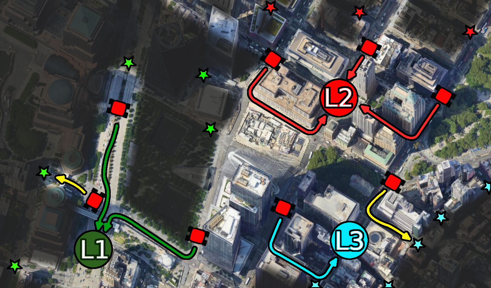
Figure 1: Intermittent communication schematics of robots meeting at rendezvous locations spread in a section of New York City. L1, L2, and L3 are our hypothetical rendezvous locations, stars from the same color are potential exploration zones near those locations, and arrows of the same color as the rendezvous indicate robots going to meet others and share maps.

Recently, [9, 10, 11] proposed approaches that aim at keeping the robots connected all the time to accomplish tasks in a known environment, while [12] propose a distributed control strategy that relies on local sensing in unknown ones. These approaches can deliver all-time communication connectivity in an MRE mission. However, keeping the robots connected is restrictive for exploration with a limited number of robots and increases exploration times. Differently, [13] makes robots decide when to deliver maps to a base-station through a Lyapunov Function and [14] allows robots to rendezvous when they have enough information.

To ensure intermittent communication, [15, 16] propose joint path planning with proximity graphs [17] allowing robots to rendezvous [18] during navigation. However, they are unfeasible for MRE because the environment is dynamic and unknown, and robots constantly update their paths to ensure robustness. A different approach would be letting them maximize the underlying DEC-POMDP by selecting promising places to explore and, at the same time, attending agreed rendezvous locations scheduled during the exploration (e.g., Fig. 1). One way to achieve scheduling in robotics is through instances of the Job Shop Scheduling Problem (JSSP) [19, 20, 21, 22] to make robots meet time constraints to collect data or to explore a region. However, to our knowledge, we have not seen such methods for frontier-based approaches.

In this paper, we propose a frontier-based method that maximizes the average reward case by exploring new locations while keeping track of where and when to rendezvous with others. Differently from [16, 11], in our approach, the robots create rendezvous agreements and explore in a distributed manner because our environment is dynamic and unknown. In this fashion, we also allow the robots to avoid the limiting constraint of full connectivity during the entire deployment. We can provide intermittent communication by first reducing the problem to instances of the JSSP that can repeat infinitely often and finding one that generates a connected proximity graph in a time interval. To avoid robots sharing maps at the same location, we propose to spread the rendezvous agreements by dynamically updating them during exploration. We further allow the robots to efficiently explore an unknown region by making them prioritize places to explore near the rendezvous locations they are assigned.

Our contributions are a frontier-based exploration method with intermittent rendezvous through agreements between robots, where each agreement specifies which and where robots should meet. We provide a method to dynamically update the rendezvous locations from the agreements to spread the exploration on the assigned mission area and a reward function for rendezvous prioritization that makes robots explore regions near their rendezvous. Furthermore, we provide means to generate the agreements automatically through a multi-objective optimization over JSSP instances obtained from reducing the MRE problem. We ensure that it provides intermittent communication because we also maximize the connectivity of its proximity graph for a time interval.

To evaluate our method, we ran a frontier-based stack in a virtual environment with several robots simultaneously. We also virtually benchmark on real-world urban maps and evaluate how many steps the robots take to explore a region. Due to the vast MRE literature, we designed two baselines based on [6, 9, 14] using a distributed frontier-based exploration method that delivers information to a base station and maintains a relay network. We show through our comparisons that our approach can explore faster without spending extra robots or relays to maintain a connected network against our baselines. We also provide a proof of concept deployment using Gazebo Simulator and the Robot Operating System (ROS).

II Problem Statement

Given a sequence of discrete time steps in the set $\mathcal{T}=\{1,2,3,...\}$ and an unknown bounded environment $\Omega\subset\mathbb{R}^{2}$, the objective of the multi-robot exploration is to deploy a group of robots from the set $\mathcal{R}=\{r_{1},...,r_{n}\}$ to explore $\Omega$ spending the minimum amount of time steps as possible. Sometimes secondary tasks are also considered, such as delivering information to a ground team through a communication network infrastructure or spreading information across all robots from $\mathcal{R}$. Frontier-based methods assist the exploration process by assigning unexplored areas into a frontier set $\mathcal{F}=\{f_{1},...,f_{k}\}$ and letting the robots pick which one to go at each time step, where each frontier represents a position inside $\Omega$. The exploration ends when there are no frontier locations to explore. While exploring, robots can avoid visiting the same places by sharing maps and their relative pose with others and doing coordination.

II-A Multi-Robot Exploration as Decentralized Partially Observable Markov Decision Process

From the perspective of a frontier-exploration method, we model the MRE setting as a Decentralized Partially Observable Markov Decision Process (DEC-POMDP) over $\Omega$, where at each time step $t\in\mathcal{T}$ a robot $r_{i}$ can select where to explore based on a state $s_{i}$ from a state set $\mathcal{S}$. We define $s_{i}$ as a tuple containing a set of all the current maps for each robot and a set of all relative poses known by each robot at time step $t$. In this model, an action comprises computing a path towards a frontier from the frontier set $\mathcal{F}_{i}$ and navigating towards it. We model the action space of each robot as $A_{i}=\{a_{1},...,a_{k},a_{k+1}\}$, where $a_{1}$ trough $a_{k}$ represent a sequence of procedures a robot executes to navigate to frontiers from $\mathcal{F}_{i}$ and $a_{k+1}$ represents an additional action that allow robot $r_{i}$ to continue executing the last action selected within ${A}_{i}\backslash a_{k+1}$. For this model, we describe the joint action space as $\mathcal{A}=A_{1}\times...\times A_{n}$. The set of transition probabilities $T$ and conditional observations $O$ are unknown. The reward function $\mathcal{R}_{reward}:\mathcal{S}\times\mathcal{A}\rightarrow\mathbb{R}$ is a real-valued function that maps the amount of area covered by the whole team per time step, where the objective is to find an action policy to select joint-actions from $A$ at each time step $t$ that maximizes the average or discounted reward.

In this paper, we propose an action inside the action set $A_{i}$ to make robots follow an intermittent communication plan. This plan ensures that maps will be shared among all team members while maximizing the average reward with an action selection policy dictated by a frontier-based exploration method. Next, we define the Intermittent Communication problem.

II-B Intermittent Communication

We model the connectivity among robots for each time step $t$ from $\mathcal{T}$ as a graph $\mathcal{G}(t)=(\mathcal{V},\mathcal{E}(t))$, where $v_{i}$ from $\mathcal{V}$ is a robot and each $e(t)=(v_{i},v_{j})$ from $\mathcal{E}(t)$ represents the connectivity between robots $v_{i}$ and $v_{j}$. We use a communication model based on a communication range $\phi$, therefore, we consider the distance between two robots to establish a communication link. At each time step, an edge $e(t)=(v_{i},v_{j})$ exists only if $||q_{i}(t)–q_{j}(t)||^{2}\leq\phi$, where $q_{i}(t),q_{j}(t)\in\Omega$ are the position of robots $v_{i}$ and $v_{j}$ at time $t$, respectively. Robots are intermittently connected only if the union of all proximity graphs $\mathcal{G}(t)$’s during an interval $[t_{n},t_{m}]$ forms a connected graph. We define the Frontier-based Multi-robot Exploration with Intermittent Connectivity problem as follows.

Problem 1

Let $\mathcal{R}$ be a set of robots exploring an unknown bounded environment $\Omega$ and let the set $\mathcal{P}_{i}=\{p_{1},p_{2},...\}$ be composed of all possible rendezvous locations for a robot $r_{i}\in\mathcal{R}$. Let the action space for robot $r_{i}$ in a DEC-POMDP be defined as $A_{i}=\{a_{1},...,a_{k+1}\}\cup\mathcal{Z}(\mathcal{P}_{i})$, such that $\mathcal{Z}:p_{j}\rightarrow a_{j}\ \forall\ p_{j}\in\mathcal{P}_{i}$ is a function that maps each rendezvous position $p_{j}$ to an action $a_{j}$ composed of finding a path and navigating through it until reaching $p_{j}$. Let the proximity graph $\mathcal{G}(t)$ represent the connectivity of robots at a time step $t$. Provide a method that maximizes the average reward represented by the sum of the area the whole team covers per time step through a frontier-based approach. Ensure that the union of all proximity graphs $\mathcal{G}(t)$ generates a connected graph for a time interval during the exploration.

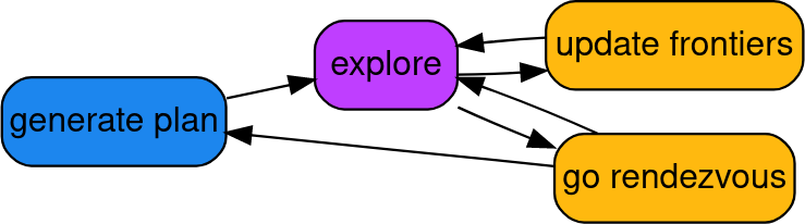
Figure 2: Simplified general overview of the rendezvous integrated as a decouple action in a frontier-based method.

III Methodology

In our method, robots explore with an intermittent communication plan with a frontier-based exploration stack, as displayed in the Finite State Machine shown in Fig. 2. During exploration, they can decide to follow an agreement with other robots generated in the generate plan state. They follow a robust frontier-based method through the explore and update frontiers states. When they meet at specific locations to honor some agreements, through the go rendezvous state. We update the team’s entire intermittent communication plan and repeat the process when appropriate. Next, we introduce how we ensure intermittent communication.

Firstly, we propose creating a rendezvous plan as actions from $A_{i}$ that are dynamically updated as exploration happens with a frontier-based method. We define a rendezvous plan with two matrices, $\mathcal{W}$ and $\mathcal{K}$, and a tuple $l=(l_{1},...,l_{f})$ composed of rendezvous locations. Columns in both matrices represent robots, rows represent rendezvous agreements, and variables from $l$ are rendezvous locations assigned to each agreement. Each $w_{ij}$ from $\mathcal{W}$ is a binary variable, where robot $r_{j}$ should participate in the $i$th agreement if $w_{ij}=1$. Differently, each $k_{ij}$ from $\mathcal{K}$ is a real value that specifies the number of exploration steps a robot should do before going to the $i$th rendezvous location in $l$.

III-1 Agreement Fulfillment and Update

Robots fulfill an agreement from the $i$th row of $\mathcal{W}$ when they meet at their assigned location from $l$. Agreements are fulfilled from the first to the last and repeat in order. Every time robots fulfill their last agreement, we dynamically update all rendezvous locations inside $l$ and distribute new plans. We purposefully let all robots participate in the last agreement from $\mathcal{W}$ and we define it as a synchronization point. We provide more insights about the synchronization later.

III-2 Agreement Maintenance during Execution

During the exploration, we maintain agreements for a robot $r_{j}$ inside a circular list and keep track of the current one with a pointer that starts at its first element. Each element of this list is a tuple $(r_{1}^{w},r_{2}^{w},...,\mathcal{L},\mathcal{Y},id)$ of the $ith$ agreement from $\mathcal{W}$, where each $r_{i}^{w}$ is the unique identifier for a robot that $r_{j}$ should meet, $\mathcal{L}$ is a value ($k_{ij}$) from $\mathcal{K}$, $\mathcal{Y}$ is the rendezvous location ($l_{i}$) of this agreement, and $id$ is the $ith$ row number. We use the row number to identify the agreement the robots have to fulfill. We initialize all $\mathcal{Y}$ for all robots with the same starting position from $\Omega$. After $r_{j}$ fulfills its current agreement, we increment the pointer to the next one on the list and follow with subsequent exploration. A robot keeps track of how much time it is effectively exploring new locations, and if this time is higher than $\mathcal{L}$, it will navigate to its current agreement rendezvous location.

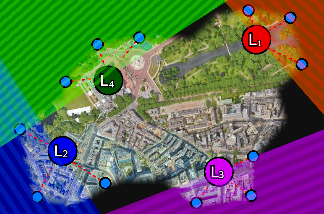
Figure 3: Example of rendezvous locations $l_{1}$ to $l_{4}$ in Buckingham Palace, London, UK. The blue circles are frontiers used by the KNN algorithm and colored zones represent the areas that robots will prioritize.

III-3 Dynamically Updating Rendezvous Locations

We dynamically update the rendezvous locations from $l$ during execution for all agreements after all robots fulfill the synchronization point. We generate the new locations by running a modified K-Nearest Neighbors (KNN) algorithm to assemble a frontier set $F_{c}=\{f_{c1},f_{c2},...\}$, where $c$ stands for centroid, based on $\mathcal{F}_{j}$ given their nearest neighbors. Next, we select which $f_{ci}$ to assign as new rendezvous location. First, we pick the farthest $f_{ci}$ from the current synchronization location and add it to a control list. We do all the subsequent selections by picking a new frontier from $F_{c}$ with the maximum distance to all others already inserted into the control list. We repeat the process until we have picked enough frontiers to update all rendezvous locations inside $l$. Fig. 3 illustrates an example of new rendezvous locations for four agreements in one of our simulated environments. Finally, we update all $\mathcal{Y}$ variables from each circular list held by the robots.

III-A Frontier Exploration with Rendezvous Prioritization

Each robot $r_{i}$ has its cell decomposition $\mathcal{C}_{i}$ obtained from $\Omega$ that can be shared with others when able to communicate and is used for planning. We will assume that a robot must find a shortest-length path $\delta(f_{i})$ in $\mathcal{C}_{i}$ to navigate towards a frontier $f_{i}$ with local and global planners.

We propose to prioritize regions in $\Omega$ to explore by considering the rendezvous locations in $l$ when robots are exploring. Let $x$ be the last rendezvous location of the synchronization point, $y$ be the rendezvous location of the current agreement of a robot. We define the reward of visiting a frontier $f_{i}$ through the following function

$$u(f_{i})=\alpha\frac{\mathcal{N}_{f_{i}}}{\Phi(f_{i})}+\beta\langle\vec{xf_{i}},\vec{yf_{i}}\rangle$$ (1)

where $\mathcal{N}_{f_{i}}$ is the total uncovered area while the robot is following $\delta(f_{i})$, $\Phi(f_{i})$ is the path length, $\vec{xf_{i}}=(f_{i}-x)$, and $\vec{yf_{i}}=(f_{i}-y)$. We use $\alpha$ and $\beta$ as scalars to regulate each term’s importance. In Fig. 3, we highlight the prioritized regions of $\Omega$ for each agreement in a rendezvous plan with locations $l_{1}$ to $l_{4}$. If the current agreement location of a robot is $l_{1}$, then it will prioritize the region highlighted with the same color as the rendezvous location. During the exploration, our method follows two strategies to select frontiers to explore, Local Coordination and Multi-robot Coordination, and we describe them as follows.

III-A1 Local Coordination Strategy

Let $\mathcal{D}$ be a set, such that each of its elements is a tuple $(f_{i},u_{i})$, where $f_{i}$ is a frontier and $u_{i}:=u(f_{i})$ its associated utility. A robot $r_{i}$ follows the local coordination strategy if there are no other robots in its communication range by finding the most promising frontier as $\{(f_{i},u_{i})\in\mathcal{D}:u_{i}\geq u_{j}\ \forall\ {(f_{j},u_{j})}\in\mathcal{D}\}$ and tries to navigate towards it using the path $\delta(f_{i})$.

	Philly	NY	DC	Tokyo	Beijing	Dubai	Moscow	Berlin	Lisbon	London	Paris	Rio
CSBS	${6760\pm 660}$	${4297\pm 606}$	${6841\pm 1221}$	${6034\pm 999}$	${6137\pm 883}$	${8336\pm 1214}$	${7069\pm 1119}$	${7337\pm 827}$	${4984\pm 521}$	${6583\pm 954}$	${6257\pm 867}$	${7367\pm 1120}$
CRN1R	${5969\pm 622}$	${3644\pm 597}$	${6426\pm 845}$	${5637\pm 903}$	${5884\pm 886}$	${7647\pm 1375}$	${7333\pm 1128}$	${6096\pm 746}$	${4895\pm 1035}$	${5777\pm 956}$	${5629\pm 669}$	${6089\pm 773}$
CRN2R	${5699\pm 680}$	${3337\pm 421}$	${6034\pm 652}$	${5116\pm 558}$	${5693\pm 751}$	${6850\pm 810}$	${5852\pm 968}$	${6154\pm 824}$	${4754\pm 811}$	${5500\pm 915}$	${5453\pm 712}$	${6063\pm 828}$
Ours	$\mathbf{4083\pm 403}$	$\mathbf{2668\pm 189}$	$\mathbf{4137\pm 244}$	$\mathbf{4030\pm 297}$	$\mathbf{3986\pm 322}$	$\mathbf{5150\pm 505}$	$\mathbf{4034\pm 368}$	$\mathbf{4276\pm 364}$	$\mathbf{3202\pm 234}$	$\mathbf{3925\pm 163}$	$\mathbf{4417\pm 382}$	$\mathbf{4108\pm 470}$
	prk01	prk02	prk03	prk04	air01	air02	air03	air04	cons01	cons02	cons03	cons04
CSBS	${5937\pm 971}$	${1799\pm 305}$	${4933\pm 1109}$	${2692\pm 461}$	${4059\pm 390}$	${6237\pm 686}$	${4452\pm 545}$	${5488\pm 999}$	${7308\pm 1126}$	${4628\pm 790}$	${5340\pm 927}$	${3865\pm 407}$
CRN1R	${5756\pm 826}$	${1709\pm 291}$	${4830\pm 881}$	${2775\pm 449}$	${4049\pm 271}$	${5739\pm 710}$	${4584\pm 453}$	${5006\pm 618}$	${6682\pm 912}$	${4215\pm 474}$	${4779\pm 601}$	${3378\pm 337}$
CRN2R	${5379\pm 533}$	${1726\pm 349}$	${4114\pm 479}$	${2948\pm 481}$	${3790\pm 288}$	${5692\pm 561}$	$\mathbf{4298\pm 330}$	${4959\pm 454}$	${6188\pm 900}$	${4126\pm 535}$	${4608\pm 527}$	${3009\pm 381}$
Ours	$\mathbf{3603\pm 389}$	$\mathbf{1624\pm 181}$	$\mathbf{3363\pm 362}$	$\mathbf{2307\pm 298}$	$\mathbf{3572\pm 394}$	$\mathbf{4812\pm 639}$	${4327\pm 489}$	$\mathbf{4137\pm 424}$	$\mathbf{4406\pm 418}$	$\mathbf{3362\pm 230}$	$\mathbf{3908\pm 524}$	$\mathbf{2827\pm 361}$

TABLE I: Benchmark results for our dataset composed of cities, parking lots (prk), airport sections (air), and constructions sites (cons).

III-A2 Multi-robot Coordination Strategy

Otherwise, if other robots are in the range of communication of $r_{i}$, we coordinate them in a distributed manner by maximizing the local Social Welfare. We define the local Social Welfare as a choice from $A$ where each robot nearby $r_{i}$ simultaneously selects a frontier to explore. Consider $\mathcal{O}=\mathcal{F}_{b}\times...\times\mathcal{F}_{z}$ as the set of all possible outcomes, where $o_{j}\in\mathcal{O}$ is a tuple containing the frontiers each nearby robot $\{r_{b},...,r_{z}\}$ should select. We approximate $\max\sum_{f\in o_{j}}u(f),\forall\ o_{j}\in\mathcal{O}$ and assign each frontier from this outcome to each robot involved in the calculation. To do this assignment, we designed a consensus algorithm based on unique identifiers. Importantly, we penalize all rewards tied to frontiers at the same location with a negative weight to prevent redundancy.

III-B Generating Rendezvous Agreements

The rendezvous plan should enable robots to connect during the exploration. However, due to differences in values from matrix $\mathcal{K}$, robots can be locked, waiting for others more often, increasing the exploration time. To make plans repeatable, we generate them in three parts. The first is the agreement, which specifies how robots should communicate over time. Differently, the second one is a reduce, making subgroups of robots meet and share maps to prepare for a full team meetup. The last part is an agreement between all robots we use to synchronize the plan, allowing a re-planing window. We propose to run an optimization procedure over a condensed proximity graph $\mathcal{G}_{c}$ and an instance $\mathcal{I}$ of the Job Shop Scheduling Problem (JSSP) [19] obtained from a reduction on a rendezvous plan. Next, we propose the following reduction.

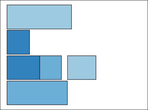
(a) Agreement

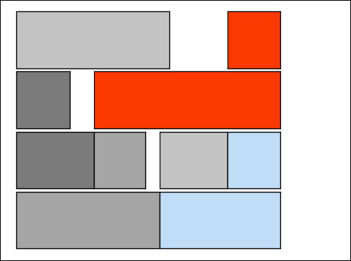
(b) Reduce

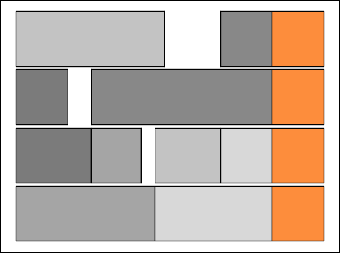
(c) Synchronize

(d) Optimized

Figure 4: Jobs with the same color allocated to different robots (lines) represent one rendezvous agreement. Robots should explore the environment until their job ends and go to the assigned rendezvous location. The X-axis represents time steps.

Before introducing our reduction algorithm, consider that machines in the JSSP instance are robots that can execute jobs. Also, consider that jobs are composed of tasks that robots should do, such as navigating and exploring a region through actions in $\mathcal{A}_{i}$.

III-B1 Reduction to JSSP Instance

Let $\mathcal{I}$ be an instance of a JSSP containing $|\mathcal{R}|$ machines that represent the rendezvous plan agreements for a sequence of time steps. Consider that $\mathcal{W}$ and $\mathcal{K}$ were given and that the execution time of a job is the total time needed to trigger a plan obtained from $\mathcal{K}$. Furthermore, consider that jobs have an identifier to show which row of $\mathcal{W}$ they are associated. We store an array $t_{\mathcal{I}}$ that holds the ending time of the previously allocated jobs for all machines and use it to create new jobs. Next, for each row $i$ of $\mathcal{W}$, we verify which robots should participate in the agreement and create a new job $j$ with length $k_{ij}$ for each. We set the starting time of each newly-created $j$ as $\max(t)$ for all participating robots to ensure locking resources, set ending time as $t_{i}+k_{ij}$, and set their identifier to $i$. We store the ending times of the current iteration inside a list $t_{e}$. Finally, we update $t_{i}$ from the participating robots as $\max(t_{e})$, store all jobs in a jobs list $J_{\mathcal{I}}$ and repeat the process until all agreements are processed.

From the JSSP instance $\mathcal{I}$, we calculate the normalized total number of jobs as

$$g_{1}(\mathcal{I})=|J_{\mathcal{I}}|\mu_{1}$$ (2)

where $\mu_{1}$ is a normalization factor; the total normalized exploration steps

$$g_{2}(\mathcal{I})=(1+\sum_{\text{job}_{i}\in J_{\mathcal{I}}}{job}_{i})^{-1}$$ (3)

where $\text{job}_{i}$ is the length of the $ith$ job from the jobs list $J_{\mathcal{I}}$; the normalized makespan

$$g_{3}(\mathcal{I})=max_{\forall t_{i}\in t_{\mathcal{I}}}(t_{i})(1+max_{\forall t_{i}\in t_{\mathcal{I}}}(t_{i}))^{-1}$$ (4)

where $t_{\mathcal{I}}$ is the ending times array we create during the reduction; and the normalized standard deviation of the distances between each agreement fulfillment

$$g_{4}(\mathcal{I})=\sigma_{\mathcal{I}}(1+\sigma_{\mathcal{I}})^{-1}$$ (5)

The intuition behind equations 2 and 4 is to quantify how often robots share maps through the number of agreements per time step. We use eq. 3 to measure how much exploration we expect to have and how much time they should explore before fulfilling their agreements through eq. 5. We exemplify the result of this reduction in Fig. 4(a) for a plan composed of four robots and three agreements. We define plan locks as situations where robots wait for others at a rendezvous location. We illustrate these locks as white gaps in the JSSP instance from Fig. 4(b).

III-B2 Reduce Agreements

Repeating the JSSP instance $\mathcal{I}$ will generate several locks because of the allocation shifts. Consequently, we generate a reduce structure to make the plan repeatable. We let the reduce be composed of $\lfloor\frac{n}{2}\rfloor$ new agreements if $n>3$, where $n$ is the number of robots. Otherwise, we create only one new agreement. To assign robots to the created agreements, we put them into a queue and do the assignment while the queue has elements. At each iteration, we process two robots, $r_{i}$ and $r_{j}$, by removing them from the queue and creating new jobs, $j_{i}$ and $j_{j}$, with the same unique job identifier. We set the starting time of $j_{i}$ and $j_{j}$ as $t_{i}$ and $t_{j}$. Differently, we set their ending times as $t_{i}+\frac{\mu_{jobs}}{2}$ and $t_{j}+\frac{\mu_{jobs}}{2}$, respectively, where $\mu_{jobs}$ is the average job length. We update each element from $t$ with the newly created jobs ending time. In Fig. 4(b), we show the procedure results for four robots when appended into the JSSP instance $\mathcal{I}$ from Fig. 4(a). The intuition behind these new agreements is to make the rendezvous plan repeatable without adding extra locks.

III-B3 Synchronize Agreement

To create a re-planning window where robots can dynamically update the entire rendezvous plan without adding locks, shifts, or undesired behaviors, we propose the concept of a synchronization agreement. Consequently, we create a new job for each robot, set their starting time to $t_{i}$ and ending time to $t_{i}+\frac{\mu_{jobs}}{2}$, and give them the same unique job identifier. We finally append all created jobs to $I$ as exemplified in Fig. 4(c).

III-B4 Optimizing the Rendezvous Plan

Let $\mathcal{H}$ be a function that generate a condensed proximity graph $\mathcal{G}=(\mathcal{V},\mathcal{E})$ that represents each time step in our JSSP instance $\mathcal{I}$. We use $\mathcal{G}$ to help evaluate the quality of the rendezvous plan. We create an edge between two robots only if they have a common agreement from $\mathcal{I}$ that can be fulfilled. From $\mathcal{G}$ we extract the connectivity index

$$g_{5}(\mathcal{I})=\mathcal{C}(\mathcal{H}(\mathcal{I}))(1+\mathcal{C}(\mathcal{H}(\mathcal{I})))^{-1}$$ (6)

where $\mathcal{C}(\mathcal{H}(\mathcal{I}))$ is a function that returns the length of the biggest connected component of $\mathcal{H}(\mathcal{I})$. We also extract the number of edges

$$g_{6}(\mathcal{I})=|\mathcal{E}_{\mathcal{H}(\mathcal{I})}|$$ (7)

where $\mathcal{E}_{\mathcal{H}(\mathcal{I})}$ is the set of edges from $\mathcal{G}$. The intuition behind eq. 6 is to see if the plan makes the robots intermittently share their maps if repeated. We use eq. 7 to count how many robots are inside the same agreement.

To generate plans, we developed a customized SGA (Simple Genetic Algorithm) [23] with genetic operators that allow us to iterate over solutions with different numbers of agreements and robots. Each individuals in the population holds a matrix $\mathcal{W}$ and $\mathcal{K}$. To evaluate them, we perform our JSSP reduction, create its condensed proximity graph, and minimize the following multi-objective optimization composed from equations 2 to 7

$$\begin{split}I^{*}=&\ \underset{\mathcal{I}}{\arg\min}\ (g_{1}(\mathcal{I}),...,g_{5}(\mathcal{H}(\mathcal{I})),g_{6}(\mathcal{H}(\mathcal{I})))\\ &\quad\text{s.t.}\\ &g_{1}(\mathcal{I}),...,g_{6}(\mathcal{H}(\mathcal{I}))\geq 0\end{split}$$ (8)

where the intuition behind this optimization is to generate a plan where the robots will keep exploring as much as possible at the cost of sharing their maps at a rate. We provide an example of a JSSP instance for a plan we generate with our method in Fig. 4(d).

IV Simulation Results

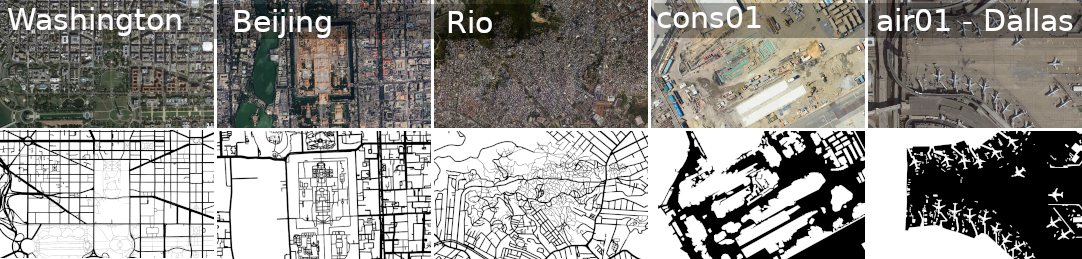
Figure 5: Samples from our benchmark and simulator. (From left to right) Washington DC, Beijing, Rio de Janeiro, construction site, Dallas International Airport.

To evaluate our method, we assembled a dataset composed of $24$ urban environments at different scales from satellite images (e.g., Fig. 5) we collected from Google Maps and prepared their cell decomposition in advance. We ran the robots in our simulator, where each robot performs a frontier exploration stack [1], and measured the total number of simulation steps to finish the exploration as done in previous MRE benchmarks [24, 25, 26]. Our experiments are: i) Benchmark: We benchmark the method against our baselines to evaluate its overall performance. ii) Consistency: We evaluate the dispersion of the results on $4$ instances of the dataset. iii) Bigger Mission Areas: We got an instance (cons01) from our dataset and doubled its dimensions to evaluate the impact of bigger areas.

We designed some baselines inspired by [6, 9, 14] to compare our method: a Constrained Static Base Station (CSBS), a Constrained Relay Network One Relay (CRN1R), and a Constrained Relay Network Two Relays (CRN2R) methods. We collected the average explored area per simulation step and its standard deviation between $10$ runs with $4$ robots for $50000$ steps each, where they have $5$ cells as visibility range and $4$ cells of communication diameter, which resembles low-spec robots. At each run, we let the robots start at the same position on the map picked randomly. The base station from the CSBS and relays have a communication range of $12$ cells on the cell decomposition. In the CRN1R each robot can place $1$ extra relay after $2000$ simulation steps at the communication boundaries to the base station or other relays, while robots in the CRN2R can place $2$ of them.

IV-1 Benchmarks Results

In Table I, we show the average number of steps robots took to complete the exploration for all $12$ environments in our dataset. The overall results suggest that our method can portray better performance than all our baselines in all city sections. They took a maximum of $5150$ and a minimum of $2668$ to explore Dubai and New York City, respectively. This behavior happened because Dubai is more structured with less feasible routes, while New York has many possible ones that facilitates the mission. For airports, parking lots, and construction sites, our method took a maximum average of $4812$ (air02) and a minimum of $1624$ (prk02). In particular, air02 has more confined structures than prk02.

IV-2 Consistency

We show the spread of the results for the cons01 and Tokyo city sections in Fig. 6. The results suggest that our method is more stable with less variation between runs. We obtained substantial gains compared to the CSBS since we spread the exploration and rendezvous through the mission area. We can also have gains by extending the base station range through relays with the CRN1R and CRN2R. However, extending this range towards infinity or keeping the robots connected might be impossible, and we expect that our method could achieve even better results for bigger areas, which we present next.

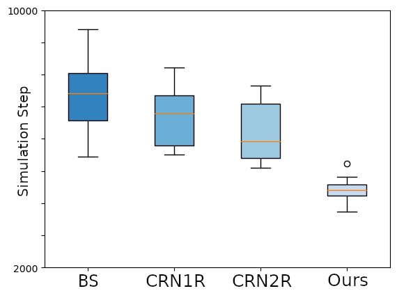
(a) cons01

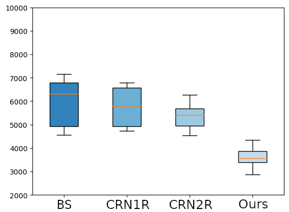
(b) prk01

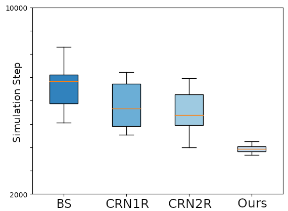
(c) London

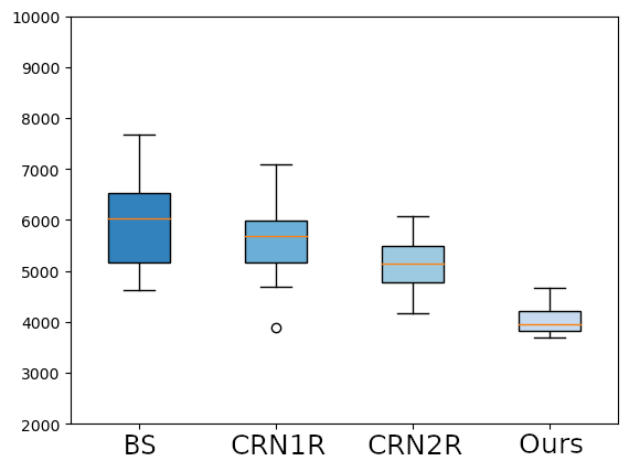
(d) Tokyo

Figure 6: Interquartile range of our baselines against our method. The Y-axis represents simulation steps.

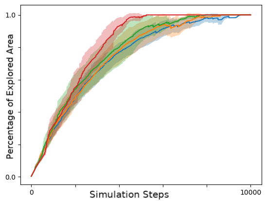
(a) cons01

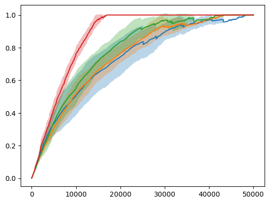
(b) cons01 scaled

Figure 7: Percentage of explored area for each simulation step. X-axis represents simulation steps and Y-axis is the percentage of area explored going from 0 to 1.

IV-3 Bigger Mission Area

Fig. 7 compares our method against the others in the cons01 instance from our dataset. We scaled its cell decomposition by $2$ in both dimensions to obtain the cons01 scaled. These results show that the other methods struggle because they have to deliver information to accomplish the mission. In contrast, the gains we see for our method are related to spreading the rendezvous across the area and making robots explore and share maps near undiscovered regions. On the other hand, the prioritized reward function we propose prevents robots from traveling long distances and provides a more steady behavior during exploration regarding the percentage of area explored per time step.

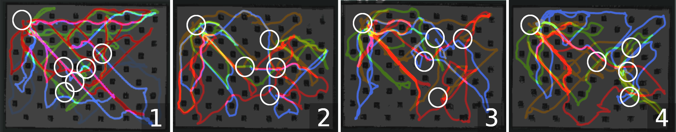
Figure 8: Traffic in rendezvous zones for $4$ trials in Gazebo simulation while executing intermittent rendezvous agreements. White circles are rendezvous locations and colored lines are trajectories.

IV-4 Gazebo Simulations

We deployed our method in non-holonomic robots using Gazebo, and we let them perform Simultaneous Localization and Mapping (SLAM) [27] with the gmapping package. We set our communication range to $2$m and stitch their maps when they can communicate. We designed a safety heuristic that reduces the robot’s velocities when near each other to prevent accidents in rendezvous zones. Our robots navigate with Roadmaps and a local planner based on Artificial Potential Fields [28]. We simplified KNN, eq. 1, and picked rendezvous updates for this deployment. We evaluated the agreement behavior in $4$ different trials.

Fig. 8, shows the overlayed trajectories of robots when executing the rendezvous agreements. We observed that the communication between robots in ROS made the integration significantly harder, and we had to design a synchronization mechanism to coordinate robots in their corresponding rendezvous agreement. Particularly, trial $1$ was the most difficult to accomplish, and we had to intervene due to rendezvous locations close to each other. Nevertheless, we show that the deployment is feasible and that we could coordinate the agreements in a distributed manner with ROS.

V Conclusion

This paper proposes a frontier-based exploration method with intermittent rendezvous. We model the problem as a DEC-POMDP to maximize the reward of visiting frontiers and propose a modification that prioritizes the ones near rendezvous locations that we update dynamically. We provide means to automatically generate rendezvous plans for several robots by reducing the MRE problem into an instance of the JSSP and optimizing it to reduce delay. We ensure intermittent communication by also maximizing the connectivity of proximity graphs obtained from this instance. To our knowledge, this is the first approach to integrate such methods to provide intermittent communication through frontier-based approaches.

We designed a benchmark of several urban environments obtained from satellite images to evaluate our method. We show through our evaluation that we can perform better without using relays. We also provide a working integration with ROS that makes little assumptions and serves as a proof-of-concept. Further research directions involve incorporating uncertainties into the model to generate better plans, deploying several decoupled ones for better coverage, or making it completely distributed.

References

- [1] F. Amigoni, J. Banfi, and N. Basilico, “Multirobot exploration of communication-restricted environments: A survey,” IEEE Intelligent Systems, vol. 32, no. 6, pp. 48–57, 2017.
- [2] K. M. Wurm, C. Stachniss, and W. Burgard, “Coordinated multi-robot exploration using a segmentation of the environment,” in 2008 IEEE/RSJ International Conference on Intelligent Robots and Systems, 2008, pp. 1160–1165.
- [3] C. M. Gifford, R. Webb, J. Bley, D. Leung, M. Calnon, J. Makarewicz, B. Banz, and A. Agah, “A novel low-cost, limited-resource approach to autonomous multi-robot exploration and mapping,” Robotics and Autonomous Systems, vol. 58, no. 2, pp. 186–202, 2010, selected papers from the 2007 European Conference on Mobile Robots (ECMR ’07). [Online]. Available: https://www.sciencedirect.com/science/article/pii/S0921889009001535
- [4] A. Bautin, O. Simonin, and F. Charpillet, “Sywap: Synchronized wavefront propagation for multi-robot assignment of spatially-situated tasks,” in 2013 16th International Conference on Advanced Robotics (ICAR), 2013, pp. 1–7.
- [5] E. A. Jensen and M. Gini, “Rolling dispersion for robot teams,” in Proceedings of the Twenty-Third International Joint Conference on Artificial Intelligence, ser. IJCAI ’13. AAAI Press, 2013, p. 2473–2479.
- [6] V. Spirin, S. Cameron, and J. de Hoog, “Time preference for information in multi-agent exploration with limited communication,” in Towards Autonomous Robotic Systems, A. Natraj, S. Cameron, C. Melhuish, and M. Witkowski, Eds. Berlin, Heidelberg: Springer Berlin Heidelberg, 2014, pp. 34–45.
- [7] L. Bravo, U. Ruiz, R. Murrieta-Cid, G. Aguilar, and E. Chavez, “A distributed exploration algorithm for unknown environments with multiple obstacles by multiple robots,” in 2017 IEEE/RSJ International Conference on Intelligent Robots and Systems (IROS), 2017, pp. 4460–4466.
- [8] L. Matignon, L. Jeanpierre, and A.-I. Mouaddib, “Coordinated multi-robot exploration under communication constraints using decentralized markov decision processes,” in Proceedings of the Twenty-Sixth AAAI Conference on Artificial Intelligence, ser. AAAI’12. AAAI Press, 2012, p. 2017–2023.
- [9] E. A. Jensen, “Restricted communication in online multi-robot exploration,” in Proceedings of the Twenty-Seventh International Joint Conference on Artificial Intelligence, IJCAI-18. International Joint Conferences on Artificial Intelligence Organization, 7 2018, pp. 5767–5768. [Online]. Available: https://doi.org/10.24963/ijcai.2018/827
- [10] P. Ong, B. Capelli, L. Sabattini, and J. Cortés, “Network connectivity maintenance via nonsmooth control barrier functions,” in 2021 60th IEEE Conference on Decision and Control (CDC), 2021, pp. 4786–4791.
- [11] ——, “Nonsmooth control barrier function design of continuous constraints for network connectivity maintenance,” Automatica, vol. 156, p. 111209, 2023. [Online]. Available: https://www.sciencedirect.com/science/article/pii/S0005109823003709
- [12] F. Pratissoli, B. Capelli, and L. Sabattini, “On coverage control for limited range multi-robot systems,” in 2022 IEEE/RSJ International Conference on Intelligent Robots and Systems (IROS), 2022, pp. 9957–9963.
- [13] L. Clark, J. Galante, B. Krishnamachari, and K. Psounis, “A queue-stabilizing framework for networked multi-robot exploration,” IEEE Robotics and Automation Letters, vol. 6, no. 2, pp. 2091–2098, 2021.
- [14] L. Bramblett, R. Peddi, and N. Bezzo, “Coordinated multi-agent exploration, rendezvous, task allocation in unknown environments with limited connectivity,” in 2022 IEEE/RSJ International Conference on Intelligent Robots and Systems (IROS), 2022, pp. 12 706–12 712.
- [15] G. A. Hollinger and S. Singh, “Multirobot coordination with periodic connectivity: Theory and experiments,” IEEE Transactions on Robotics, vol. 28, no. 4, pp. 967–973, 2012.
- [16] H. Rovina, T. Salam, Y. Kantaros, and M. Ani Hsieh, “Asynchronous adaptive sampling and reduced-order modeling of dynamic processes by robot teams via intermittently connected networks,” in 2020 IEEE/RSJ International Conference on Intelligent Robots and Systems (IROS), 2020, pp. 4798–4805.
- [17] F. Bullo, J. Cortes, and S. Martinez, Distributed Control of Robotic Networks: A Mathematical Approach to Motion Coordination Algorithms. USA: Princeton University Press, 2009.
- [18] Y. Kantaros, M. Guo, and M. M. Zavlanos, “Temporal logic task planning and intermittent connectivity control of mobile robot networks,” IEEE Transactions on Automatic Control, vol. 64, no. 10, pp. 4105–4120, 2019.
- [19] K. Gao, Z. Cao, L. Zhang, Z. Chen, Y. Han, and Q. Pan, “A review on swarm intelligence and evolutionary algorithms for solving flexible job shop scheduling problems,” IEEE/CAA Journal of Automatica Sinica, vol. 6, no. 4, pp. 904–916, 2019.
- [20] Y. Fang, C. Peng, P. Lou, Z. Zhou, J. Hu, and J. Yan, “Digital-twin-based job shop scheduling toward smart manufacturing,” IEEE Transactions on Industrial Informatics, vol. 15, no. 12, pp. 6425–6435, 2019.
- [21] R. Li, W. Gong, L. Wang, C. Lu, and C. Dong, “Co-evolution with deep reinforcement learning for energy-aware distributed heterogeneous flexible job shop scheduling,” IEEE Transactions on Systems, Man, and Cybernetics: Systems, pp. 1–11, 2023.
- [22] W. Song, X. Chen, Q. Li, and Z. Cao, “Flexible job-shop scheduling via graph neural network and deep reinforcement learning,” IEEE Transactions on Industrial Informatics, vol. 19, no. 2, pp. 1600–1610, 2023.
- [23] K. Tang, K. Man, S. Kwong, and Q. He, “Genetic algorithms and their applications,” IEEE Signal Processing Magazine, vol. 13, no. 6, pp. 22–37, 1996.
- [24] J. Faigl and M. Kulich, “On benchmarking of frontier-based multi-robot exploration strategies,” in 2015 European Conference on Mobile Robots (ECMR), 2015, pp. 1–8.
- [25] U. Jain, R. Tiwari, and W. W. Godfrey, “Comparative study of frontier based exploration methods,” in 2017 Conference on Information and Communication Technology (CICT), 2017, pp. 1–5.
- [26] N. Payandeh, F. Mehrabi, R. Fesharakifard, and Y. AlizadehVaghasloo, “A comparison between rapidly randomized tree and efficient frontier methods for autonomous mobile robot exploration,” in 2022 10th RSI International Conference on Robotics and Mechatronics (ICRoM), 2022, pp. 466–471.
- [27] M. Dissanayake, P. Newman, S. Clark, H. Durrant-Whyte, and M. Csorba, “A solution to the simultaneous localization and map building (slam) problem,” IEEE Transactions on Robotics and Automation, vol. 17, no. 3, pp. 229–241, 2001.
- [28] C. Warren, “Global path planning using artificial potential fields,” in Proceedings, 1989 International Conference on Robotics and Automation, 1989, pp. 316–321 vol.1.