Portrait Stylization: Artistic Style Transfer with
Auxiliary Networks for Human Face Stylization

Abstract

Today’s image style transfer methods have difficulty retaining humans face individual features after the whole stylizing process. This occurs because the features like face geometry and people’s expressions are not captured by the general-purpose image classifiers like the VGG-19 pre-trained models. This paper proposes the use of embeddings from an auxiliary pre-trained face recognition model to encourage the algorithm to propagate human face features from the content image to the final stylized result.

1 Introduction

The style transfer technique is currently one of the most studied areas in deep learning applied to digital art. It consists in reconstructing a given content image – the image that will seed the overall structure of the resulting image, e.g. an animal, a landscape or a human portrait – with the style of a given style image – the image that will seed the texture of the resulting image, e.g. an oil painting or an abstract art – producing the final stylized result image output.

This technique made possible new forms of digital art, like reproducing classical paintings with the content of modern days or creating amazing new effects that weren’t previously possible. Despite that, actual state-of-the-art algorithms show limitations when applied to images with human faces. These methods yield face deformations in the final result image, which makes it difficult to recreate portrait paintings such as The Mona Lisa from Leonardo da Vinci or Self Portrait from Vincent Van Gogh.

The main cause of this is that the human face geometry is not passed as an important content criterion, as the VGG-Network [Simonyan and Zisserman 2015] can’t capture so much relevant features about the human face. This problem can be solved by simply using a face recognition model like FaceNet [Schroff et al. 2015] as an auxiliary model for content feature extraction. So, in that way, the human face geometry and other relevant facial features can be propagated to the final result image.

2 Background

This problem can be formulated as Finding the optimal changes for a content image that minimizes the difference between its texture and the texture from a style image without losing the high-level information contained in it. These content and style differences can be calculated through the internal representations of a pre-trained deep convolutional neural network like the VGG-Network given that, following the paper A Neural Algorithm of Artistic Style [Gatys et al. 2015], the higher layers from these networks can capture high-level information – like textures and color palettes – from its input images, at the same time that its lower layers can capture low-level information like the object’s geometry and its colors.

There are many ways of finding these optimal changes, but here the focus goes to the traditional optimization technique. This technique was first introduced by Gatys’ 2015 paper and uses the quasi-Newton optimization algorithm Limited-memory BFGS optimizer [Liu and Nocedal 1989] to solve the style transfer problem by optimizing the pixels of an initial image, that can be a noise or the own content image, in the same way that the weights of a deep learning model are optimized, through the minimization of a criterion function (Eq. 1).

This criterion function is the weighted sum between a content loss function (Eq. 3) and a style loss function (Eq. 6), This means that the content and style weights can be controlled by $\alpha$ and $\beta$ factors respectively, giving the user more control over the result image. The function is defined as follows:

$$\mathcal{L}_{total}(\vec{c},\vec{s},\vec{x})=\alpha\mathcal{L}_{content}(\vec{c},\vec{x})+\beta\mathcal{L}_{style}(\vec{s},\vec{x})$$ (1)

Where $\vec{c}$ is the content image, $\vec{s}$ the style image and $\vec{x}$ the result image.

2.1 Content Loss

The content of a given image can be represented by the responses from convolutional filters of lower layers in a pre-trained VGG-Network that will be called here feature representations. The responses from a given layer $l$ can be stored in a matrix $F^{l}\in\mathbb{R}^{N_{l}\times M_{l}}$ where $N_{l}$ represents the number of filters contained in layer $l$, $M_{l}$ represents the number of pixels – product between width and height – of the filters contained in layer $l$, and $F^{l}_{ij}$ are the output activations from the $i^{th}$ filter at position $j$ from layer $l$.

In that way, the content loss function for a given layer $l$ can be defined as the mean squared error between the content image feature representations $C^{l}$ and the result image feature representations $X^{l}$:

$$\mathcal{L}_{content}(\vec{c},\vec{x},l)=\frac{1}{N}\sum_{i,j}^{N}(C^{l}_{ij}-X^{l}_{ij})^{2}$$ (2)

Then, being $L$ the total number of content layers and $W_{l}^{c}$ the relative weight of content layer $l$, the final content loss function can be calculated by the weighted sum of all the content layer losses:

$$\mathcal{L}_{content}(\vec{c},\vec{x})=\sum_{l=0}^{L}W_{l}^{c}\times\mathcal{L}_{content}(\vec{c},\vec{x},l)$$ (3)

2.2 Style Loss

Like the content feature representations, the style of a given image is also represented by the responses from convolutional filters of a pre-trained VGG-Network. Nevertheless, it is actually represented by higher layers of the network and not directly, but through the correlations between the filter responses. These correlations are given by the Gram Matrix $G^{l}\in\mathbb{R}^{N_{l}\times N_{l}}$, where:

$$G^{l}_{ij}=\sum_{k}F^{l}_{ik}\times F^{l}_{jk}$$ (4)

From that way, the style loss function from a given layer $l$ can be defined as the mean squared error between the Gram Matrix of layer $l$ from the style image $S^{l}$ and the Gram Matrix of layer $l$ from the result image $A^{l}$:

$$\mathcal{L}_{style}(\vec{s},\vec{x},l)=\frac{1}{4N_{l}^{2}M_{l}^{2}}\sum_{i,j}(S^{l}_{ij}-A^{l}_{ij})^{2}$$ (5)

Finally, being $L$ the total number of style layers and $W_{l}^{s}$ the relative weight of style layer $l$, the final style loss function can be calculated by the weighted sum of all the style layer losses:

$$\mathcal{L}_{style}(\vec{s},\vec{x})=\sum_{l=0}^{L}W_{l}^{s}\times\mathcal{L}_{style}(\vec{s},\vec{x},l)$$ (6)

2.3 The Problem of High Resolution

Beautiful synthetic images can be generated by applying the Gatys’ method to a given content image and style image, like the ones at Figure 1.

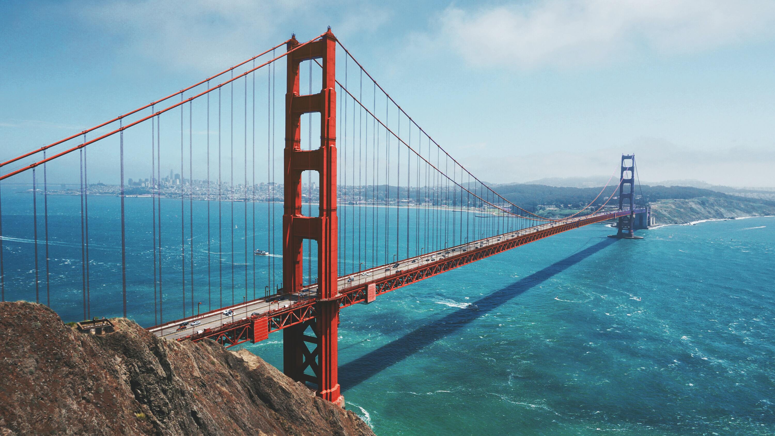
(a) Content Image

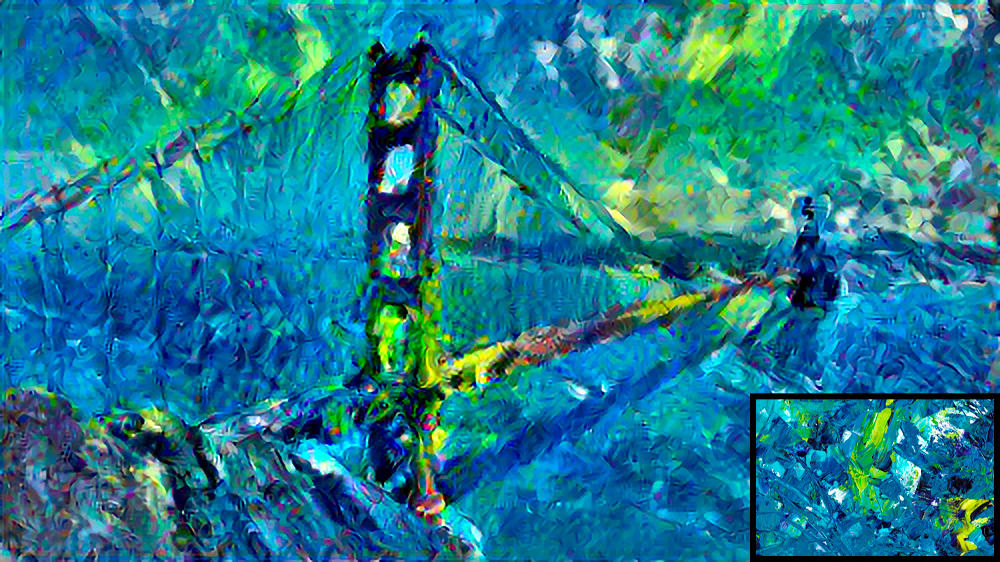
(b) Style 1

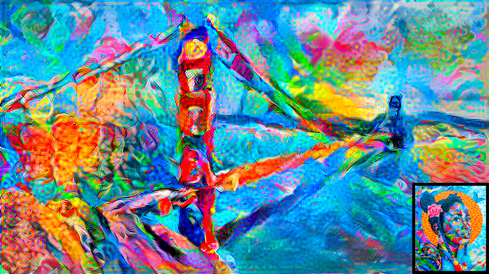
(c) Style 2

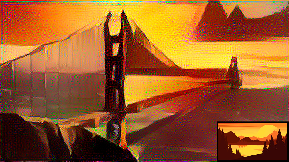
(d) Style 3

Figure 1: An image from The Golden Gates Bridge stylized with different style images through the Gatys’ 2015 method. All samples are generated at a 500px resolution, and each style used is minimized at the right-bottom edge of each sample.

Nevertheless, this method has limitations when applied to high resolution images (e.g. 1080px or 1440px), resulting in only some color changes and almost no structural change (Figure 2). This phenomenon occurs because the receptive fields of convolutional neural networks have fixed sizes, and in higher-resolution images its becomes relatively small, what makes the VGG-Network to pay attention only to small structures of the image during the stylization process, ignoring the overall image structure.

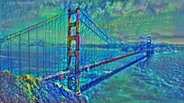
(a) Style 1

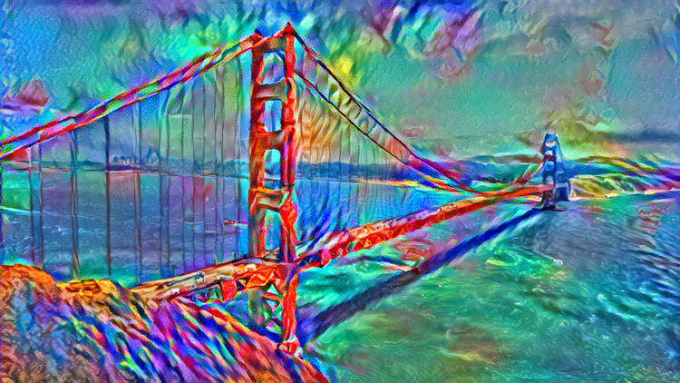
(b) Style 2

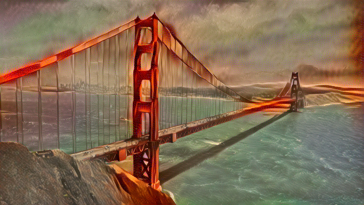
(c) Style 3

Figure 2: An image from The Golden Gates Bridge stylized with the respective style images from Figure 1 in high resolution (1080px). These samples show the limitations of the method when applied to high-resolution images.

Following the paper Controlling Perceptual Factors in Neural Style Transfer  [Gatys et al. 2016], the optimal resolution size of input images when using the VGG-Network for style transfer is around 500px, where bigger structural changes occurs while image content is well-preserved, like in Figure 1(c).

3 Improving the Quality of the Generations

The Gatys’ 2016 paper also proposes that the quality of generations at high resolution can be improved through the coarse-to-fine technique. It consists of dividing the stylizing process into two stages, where given a high-resolution content and style images $\vec{c}$ and $\vec{s}$ with $N$ number of pixels, is defined by the following processes:

In the first stage, the images are downsampled by a $K$ factor, such that $N/K$ corresponds to the resolution where the stylization will be performed, e.g. $500^{2}$px for VGG-Network. After this process, the stylization is performed with the downsampled images, generating a low-resolution result image $\vec{z}$.

Now, at the second stage, the generated image $\vec{z}$ is upsampled to $N$ pixels and then used as initial image for the stylization process of the original input images $\vec{c}$ and $\vec{s}$, generating the final result image $\vec{x}$. This process causes the algorithm to fill in the high-resolution information without losing the overall style structure of the $\vec{z}$ image (Figure 3(b)).

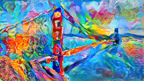
(a) Low resolution (500px)

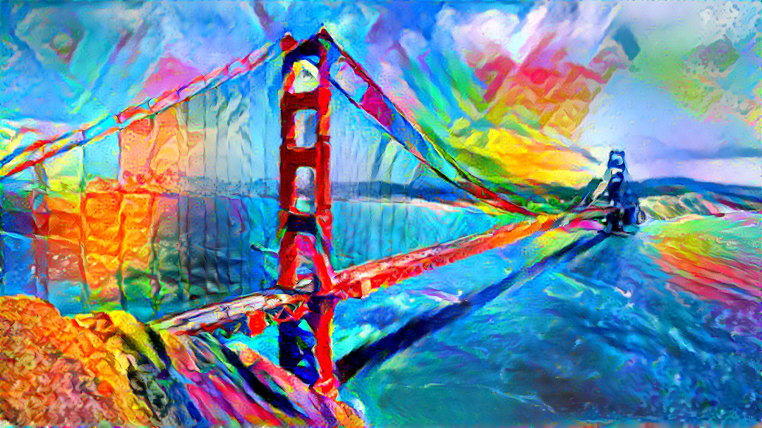
(b) Upsampled (1080px)

Figure 3: An example of the coarse-to-fine process applied to The Golden Gates Brigde stylized image from Figure 1(c).

The method proposed in this paper is based on Crowson’s Neural Style Transfer implementation [Crowson 2021]. Various relevant changes were made to the stylizing process to improve the quality of the generated images, but here only some of those will be discussed.

First, the coarse-to-fine technique is divided into $s$ stages, rather than one stage for low-resolution stylization and another to high-resolution one. The stylization process is started at an initial resolution $r_{i}$ and then is applied to progressively larger scales, each greater by a factor $k=\sqrt{2}$ until it reaches a final resolution $r_{f}$. In this way, the resolution $R(s)$ at a given stage $s$ is defined as:

$$R(s)=\min\{r_{f},r_{i}\times k^{s-1}\}$$ (7)

To improve the use of available memory, the Adam optimizer [Kingma and Ba 2015] is used instead of the L-BFGS optimizer, which allows the processing of higher resolution images while still producing similar results.

The algorithm’s style perception can be improved to yield more expressive results by setting a different weight for each style layer. The layers used for stylization are the same as in Gatys’ 2015 method: relu1_1, relu2_1, relu3_1, relu4_1 and relu5_1, and the weights assigned to respectively each layer is $256,64,16,4$ and $1$, what is then normalized through the softmax function.

To approximate the effects of gradient normalization and produce better visual effects, a variation of the mean squared error function is used to compute the content and style losses. Here, the traditional squared error is divided by the sum of the absolute difference of the inputs, in a way that the gradient L1-norm of the resulting function will be $\approx 1$. For a given input $y$, a target $\hat{y}$ and an $\epsilon=1\mathrm{e}{-8}$ value to avoid zero divisions, the normalized squared error function is defined as:

$$NSE(y,\hat{y})=\frac{\sum_{i}(y_{i}-\hat{y}_{i})^{2}}{\sum_{i}|y_{i}-\hat{y}_{i}|+\epsilon}$$ (8)

The Gram Matrix for style representation was also changed. Now it is normalized by the number of filters contained in each style layer:

$$G^{l}_{ij}=\frac{\sum_{k}F^{l}_{ik}\times F^{l}_{jk}}{N_{l}}$$ (9)

Finally, following the paper Understanding Deep Image Representations by Inverting Them [Mahendran and Vedaldi 2014], spatial smoothness in the resulting image $\vec{x}$ can be encouraged by the L2 total variation loss, defined as:

$$TV_{loss}(\vec{x})=\frac{1}{N}\sum_{i,j}^{N}\Bigl{(}(\vec{x}_{i,j+1}-\vec{x}_{ij})^{2}+(\vec{x}_{i+1,j}-\vec{x}_{ij})^{2}\Bigr{)}$$ (10)

So, it is summed with the content and style losses with a weight control value $\gamma$, defining the final total loss as:

$$\mathcal{L}_{total}(\vec{c},\vec{s},\vec{x})=\alpha\mathcal{L}_{content}(\vec{c},\vec{x})+\beta\mathcal{L}_{style}(\vec{s},\vec{x})+\gamma TV_{loss}(\vec{x})$$ (11)

With all these changes and a few others that can be found in Crowson’s repository, the results of the style transfer process are even improved, resulting in smoother images, with well-preserved content and more expressive strokes (Figure 4(b)).

(a) Gatys et al.

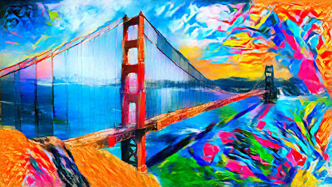
(b) K. Crowson

Figure 4: Comparison between the Gatys’ 2016 style transfer method before (a) and after (b) Crowson’s changes. After these improvements, the image content becomes well-preserved while the stylized regions are more expressive.

3.1 Limitations

Despite those improvements, the method still produces facial deformations when applied to content images with human faces (Figure 5(c)), as the content layer relu4_2 can’t output meaningful representations of human facial features.

(a) Content Image

(b) Style Image

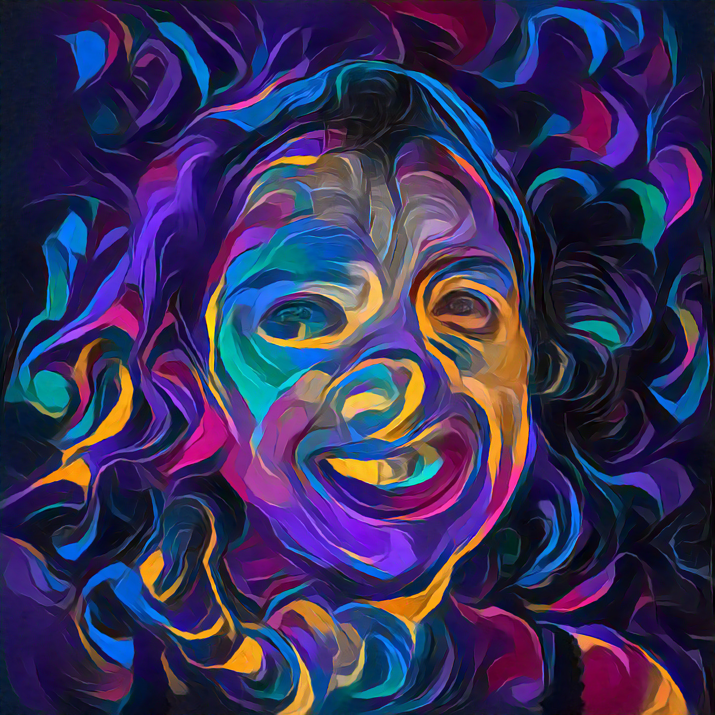
(c) K. Crowson

Figure 5: A failure case of the Crowson’s method, where the facial features of the content image are not propagated to the final result image, making the face contained in the result unrecognizable.

These distortions in the generated results (Figure 5(c)) occurs because the VGG-Network layers used for content extraction (relu4_2 in the Gatys’ and Crowson’s methods) can’t output meaningful activations about human faces when exposed to it, as this network was trained for the general-purpose image classification task and not for domain-specific tasks like face recognition.

4 Proposed Method

This paper proposes a new method, that will be called as Portrait Stylization, to solve the face distortion problem in Crowson’s algorithm. It solves the problem by adding to the total loss function a new domain-specific content loss, called here as FaceID loss, that uses the responses from the convolutional filters of a pre-trained face recognition algorithm, like the state-of-the-art FaceNet [Schroff et al. 2015], to compute the difference between the facial features of the content image $\vec{c}$ and the result image $\vec{x}$.

These responses are extracted from an Inception-Resnet-V1 FaceNet model, pretrained on the VGGFace2 [Cao et al. 2017] dataset, and will be called here as facial features. The layers selected for extracting these facial features are: conv_1a, conv_2a, maxpool_3a, conv_4a and conv_4b, with the same weight assigned to each one. It was empirically selected, following the idea that higher layers in a feed-forward convolutional neural network architecture are better in extracting general-features.

The FaceID loss function can be defined as the weighted sum of the normalized squared error (Eq. 8) between the content image facial features $C^{l}$ and the result image facial features $X^{l}$, being $W_{l}^{f}$ the weight for a given FaceNet layer $l$:

$$\mathcal{L}_{facial}(\vec{c},\vec{x})=\delta\times\sum_{l=0}^{L}W_{l}^{f}\times NSE(C^{l},X^{l})$$ (12)

Where $\delta$ is the face weight value, that gives the user control of how similar the faces contained in the result image will be in comparison to the faces in the content image.

This auxiliary criterion helps the algorithm retain the facial features of the human faces in the content image after the stylizing process, which avoids drastic facial deformations while still producing expressive stylization results (Figure 6(b)).

(a) K. Crowson

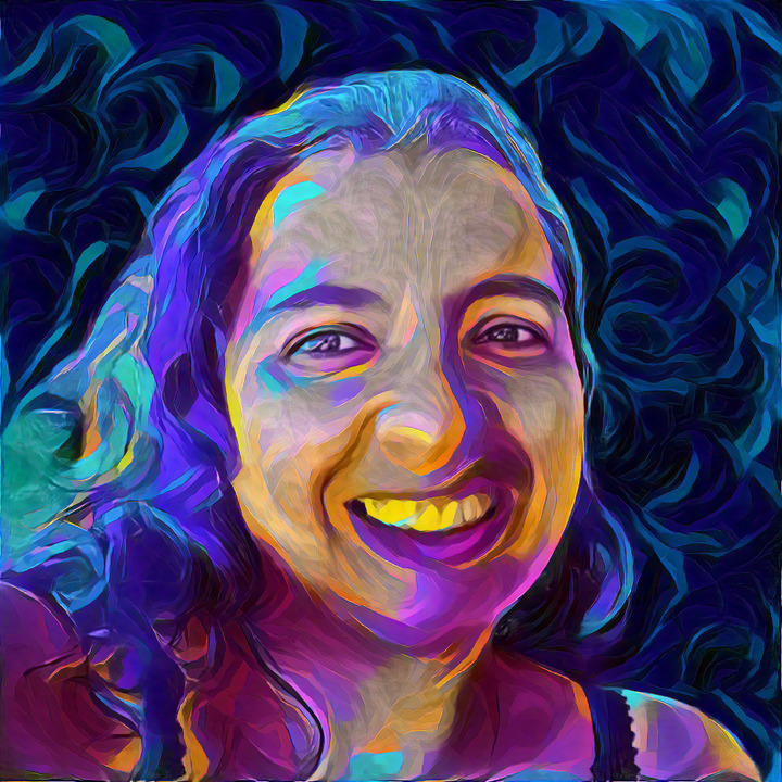
(b) P.S. Method

Figure 6: Comparison between the Crowson’s style transfer method before (a) and after (b) the addition of the FaceID Loss.

Nevertheless, even with those improvements, using only the facial features as a criterion for the face reconstruction don’t give the user much control about the style of result image, as the style strokes becomes lower expressive as the $\delta$ value increases (Figure 7).

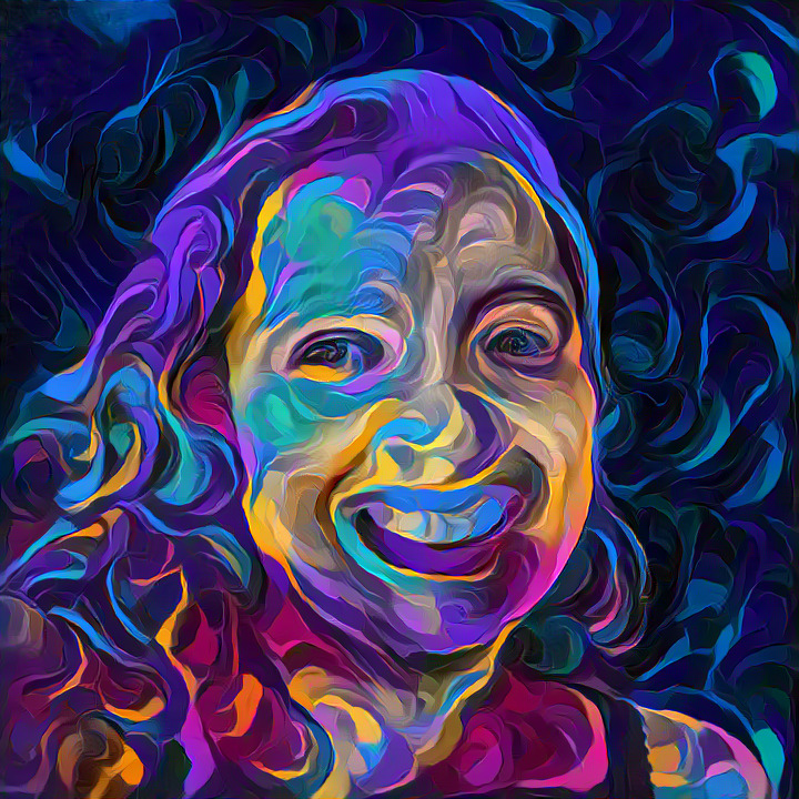
(a) $\delta=0.05$

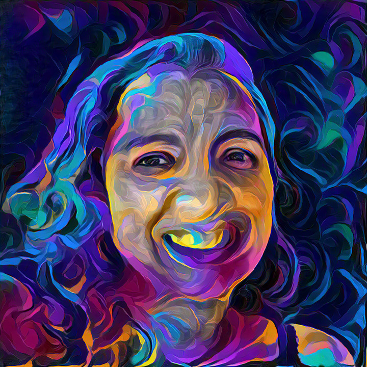
(b) $\delta=0.15$

(c) $\delta=0.25$

(d) $\delta=0.35$

(e) $\delta=0.45$

Figure 7: Changes caused by the FaceID loss, from $\delta=0.05$ until $\delta=0.45$, with a step size of $\Delta=0.1$. All these experiments use $\alpha=0.05$ and $\beta=1.0$, with the same content and style images from Figure 5.

In that way, to improve the control of the face geometry in the result image while maintaining the expressive stylization results, the differentiable output from the FaceMesh [Kartynnik et al. 2019] algorithm can be used to compute the difference between the surface geometry of the faces contained in the content and result images.

The FaceMesh algorithm is a feed-forward convolutional neural network trained to approximate a 3D mesh representation of human faces from only RGB image inputs (Figure 8). It outputs a relatively dense mesh model of 468 vertices that was designed for face-based augmented reality effects.

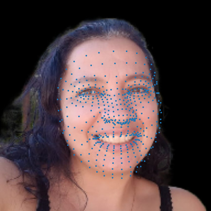
(a)

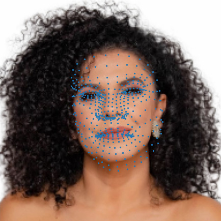
(b)

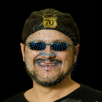
(c)

Figure 8: Examples of mesh models generated by the FaceMesh algorithm applied to content images with real human faces. To produce high-precision meshes, the faces on the input image need to be cropped and resized to 192x192 resolution.

So, the new FaceID loss can be defined by adding to the old one the normalized squared error (Eq. 8) between the content mesh model $C_{M}$ and the result mesh model $X_{M}$:

$$\mathcal{L}_{facial}(\vec{c},\vec{x})=\eta NSE(C_{M},X_{M})+\delta\sum_{l=0}^{L}W_{l}^{f}\times NSE(C^{l},X^{l})$$ (13)

Where $\eta$ is the meshes weight value, that gives the user control of how much similar the surface geometry of faces contained in the result image will be in relation to the ones in the content image.

This encourages the algorithm to reproduce the face geometries contained on the content image, on the result image, while still allows it to produce expressive strokes, as the other facial features like the skin texture or micro expressions is not represented by the mesh model.

(a) $\delta=0.00,\eta=0.00$

(b) $\delta=0.00,\eta=0.015$

(c) $\delta=0.25,\eta=0.00$

(d) $\delta=0.25,\eta=0.015$

Figure 9: Changes caused by the new FaceMesh term in different algorithm settings. All these experiments use $\alpha=0.05$ and $\beta=1.0$, with the same content and style images from Figure 5.

This new term improves the quality of face reconstructions in the result image even when it is used alone. When used jointly with the facial features (with $\delta>0.00$), makes the algorithm produce even better results, helping the user to adjust fine facial geometry details like the nose or mouth formats, producing facial expressions most similar to the ones in the content image (Figure 9(d)).

5 Image Preprocessing

To improve the stylization results of the algorithms used here, making it focus only on the faces contained in the content image and avoiding possible confusion caused by the background texture, the background was removed and replaced by a flat color through the MODNet Trimap-Free Portrait Matting [Ke et al. 2020] algorithm (Figure 10).

(a) Original

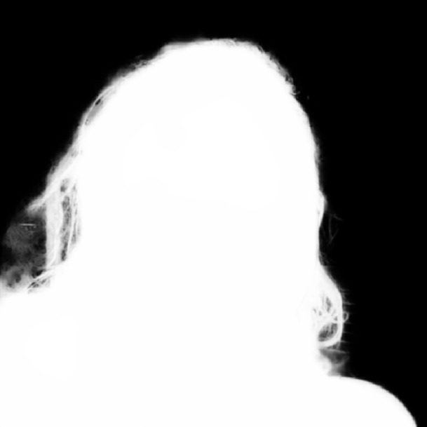
(b) Mask

(c) Result

Figure 10: An example of a content image before (a) and after (c) the background removal process. All the black pixels in the mask (b) are replaced by a black color in the resulting image, and the white pixels are maintained with the same color values.

This step is not needed by the algorithms, but it improves their overall performance in portrait images. The Portrait Stylization method can generate an image with only a few facial distortions even with its background, but the other algorithms seem to yields bigger distortions when applied to this same case (Figure 11).

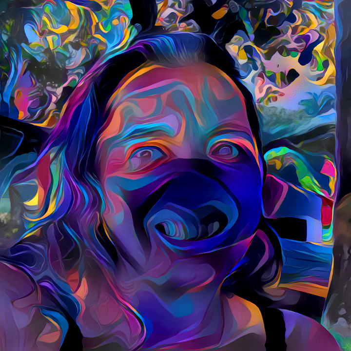
(a) Gatys et al.

(b) K. Crowson

(c) P.S. Method

Figure 11: The results of stylizing a portrait image without removing its background. To generate these samples, the same style image and hyperparameters from Figure 9(d) were used.

6 Style Transfer with Multiple Face Portraits

To enable the support of stylizing images that contain more than one human face, a few changes need to be made to the algorithm. A face detection algorithm like the state-of-the-art MTCNN [Zhang et al. 2016] is used to extract the coordinates of the faces contained in the content image. With this coordinates, the facial regions in the content and result images are cropped, generating sub-images from the ground truth and generated faces (Figure 12).

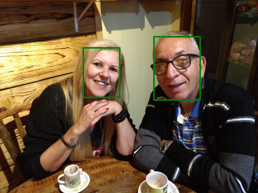
(a) Content Image

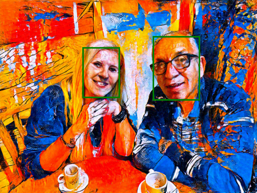
(b) Result Image

Figure 12: An example of how the MTCNN algorithm extracts the face coordinates from the content image and uses them to crop the faces in the result image. This process ensures that the faces in the generated image will always be detected, no matter what changes the styling process does.

The facial features of all these sub-images are extracted through the FaceNet and FaceMesh models. The features from the content image faces are concatenated layer by layer, generating a tuple of vectors $G$ that represents the ground truth facial geometries of all faces. At the same time, the extracted features from the result image faces are too concatenated layer by layer, generating a tuple of vectors $H$ that represents the actual geometries of the faces in the generated image.

After these processes, the FaceID Loss are calculated using these concatenated vectors as facial representations rather than using the facial features extracted from the entire image pixels.

$$\mathcal{L}_{facial}(\vec{c},\vec{x})=\eta NSE(G_{M},H_{M})+\delta\sum_{l=0}^{L}W_{l}^{f}\times NSE(G_{f}^{l},H_{f}^{l})$$ (14)

Where $G_{M}$ and $G_{f}^{l}$ are the concatenated mesh models and facial features from the faces in the content image, and $H_{M}$ and $H_{f}^{l}$ are the concatenated mesh models and facial features from the faces in the result image.

7 Performance Comparisons

The Portrait Stylization method produces significant visual improvements, compared to the current state-of-the-art methods, when applied to images that contain human faces (Table 1). This still can be applied to any other image types as the method becomes exactly the same as Crowson’s method when $\delta=0.00$ and $\eta=0.00$.

#	Input	Gatys et al.	K. Crowson	P.S. Method
1
2
3
4

Table 1: Some experiments were made to compare the performance between the Gatys’ 2016 method, the Crowson’s method and the Portrait Stylization method when applied to portrait images. The content and style image of each sample is shown in the Input column.

8 Conclusion

This paper proposes improvements to the Crowson’s algorithm to improve the quality of the results in images that contain one or more human faces. These improvements show that this algorithm can be optimized for specific image groups (e.g. portraits, cars, or animals) through changes in the total loss function.

The addition of auxiliary models, pre-trained on domain-specific tasks, can help the stylization process giving the user more control over how the style and content will be merged in the generated image. So, in the same way that face detectors can help in the portrait styling process, other domain-specific models like a pre-trained pose-estimation algorithm, could help in the stylization of full-body images.

This is a great experiment to explore in future research, jointly with the possibility of fine-tuning the VGG-Network with a stacked dataset of open-domain and specific-domain images. This could enable a single content extraction model, optimizing the memory usage and the speed of the whole stylization process.

References

- [Cao et al. 2017] Cao, Q., Shen, L., Xie, W., Parkhi, O. M., and Zisserman, A. (2017). Vggface2: A dataset for recognising faces across pose and age. CoRR, abs/1710.08092.
- [Crowson 2021] Crowson, K. (2021). An implementation of neural style transfer (a neural algorithm of artistic style) in pytorch. https://github.com/crowsonkb/style-transfer-pytorch/tree/1107fe68639a59bd54bcda018e25dd770819ab19.
- [Gatys et al. 2015] Gatys, L. A., Ecker, A. S., and Bethge, M. (2015). A neural algorithm of artistic style. CoRR, abs/1508.06576.
- [Gatys et al. 2016] Gatys, L. A., Ecker, A. S., Bethge, M., Hertzmann, A., and Shechtman, E. (2016). Controlling perceptual factors in neural style transfer. CoRR, abs/1611.07865.
- [Kartynnik et al. 2019] Kartynnik, Y., Ablavatski, A., Grishchenko, I., and Grundmann, M. (2019). Real-time facial surface geometry from monocular video on mobile gpus. CoRR, abs/1907.06724.
- [Ke et al. 2020] Ke, Z., Li, K., Zhou, Y., Wu, Q., Mao, X., Yan, Q., and Lau, R. W. H. (2020). Is a green screen really necessary for real-time portrait matting? CoRR, abs/2011.11961.
- [Kingma and Ba 2015] Kingma, D. P. and Ba, J. (2015). Adam: A method for stochastic optimization. In Bengio, Y. and LeCun, Y., editors, 3rd International Conference on Learning Representations, ICLR 2015, San Diego, CA, USA, May 7-9, 2015, Conference Track Proceedings.
- [Liu and Nocedal 1989] Liu, D. C. and Nocedal, J. (1989). On the limited memory bfgs method for large scale optimization. Math. Program., 45.
- [Mahendran and Vedaldi 2014] Mahendran, A. and Vedaldi, A. (2014). Understanding deep image representations by inverting them. CoRR, abs/1412.0035.
- [Schroff et al. 2015] Schroff, F., Kalenichenko, D., and Philbin, J. (2015). Facenet: A unified embedding for face recognition and clustering. CoRR, abs/1503.03832.
- [Simonyan and Zisserman 2015] Simonyan, K. and Zisserman, A. (2015). Very deep convolutional networks for large-scale image recognition. In Bengio, Y. and LeCun, Y., editors, 3rd International Conference on Learning Representations, ICLR 2015, San Diego, CA, USA, May 7-9, 2015, Conference Track Proceedings.
- [Zhang et al. 2016] Zhang, K., Zhang, Z., Li, Z., and Qiao, Y. (2016). Joint face detection and alignment using multi-task cascaded convolutional networks. CoRR, abs/1604.02878.