Epidemic Forecast Follies

Abstract

We introduce a simple multiplicative model to describe the temporal behavior and the ultimate outcome of an epidemic. Our model accounts, in a minimalist way, for the competing influences of imposing public-health restrictions when the epidemic is severe, and relaxing restrictions when the epidemic is waning. Our primary results are that different instances of an epidemic with identical starting points have disparate outcomes and each epidemic temporal history is strongly fluctuating.

I Background

Now that the most severe (we hope) manifestations of the Covid-19 epidemic have passed, one can’t help but realize that many of the early forecasts of the Covid-19 epidemic toll were wildly inaccurate and inconsistent with each other. Moreover, individual forecasts could change dramatically over a period of few days. For the USA, in particular, the earliest estimates for the Covid-19 epidemic death toll ranged from tens of thousands to many millions, with the current death toll (as of September 2023) reported to be 1.175 million out of a total of 108.5 million cases (all data taken from Cov (2023)). Perhaps even more striking are the huge fluctuations and the dramatically different time courses in the daily death rate in different countries.

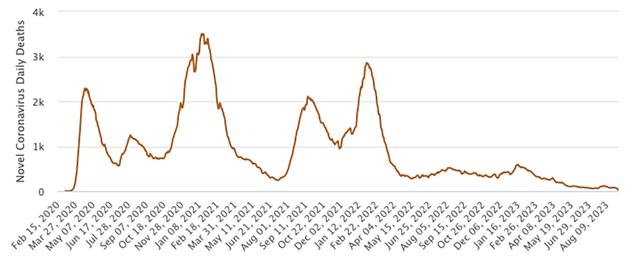
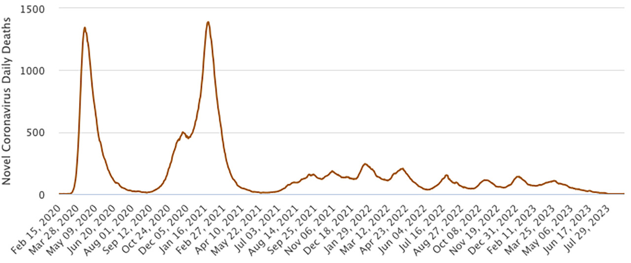
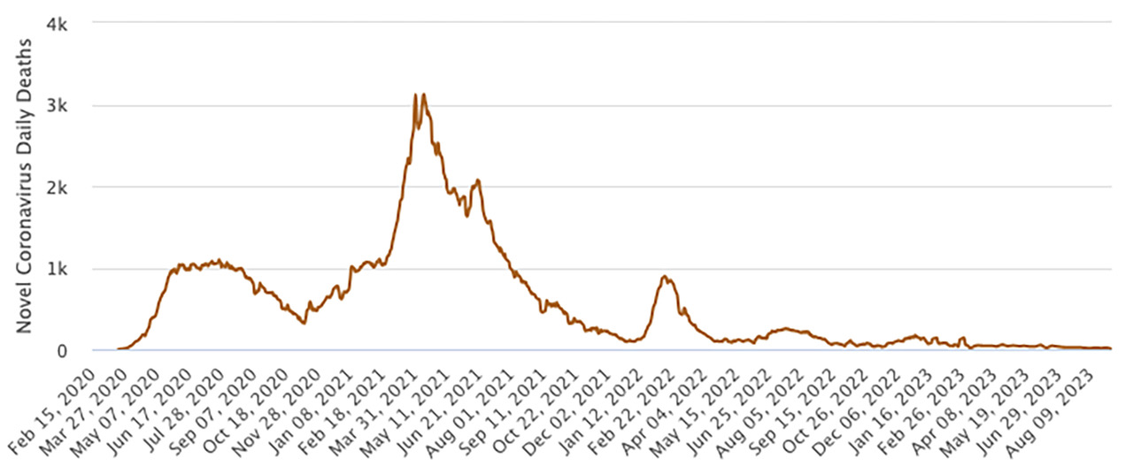
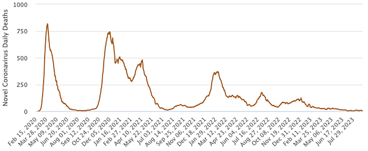
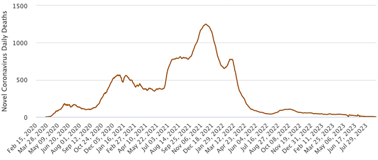
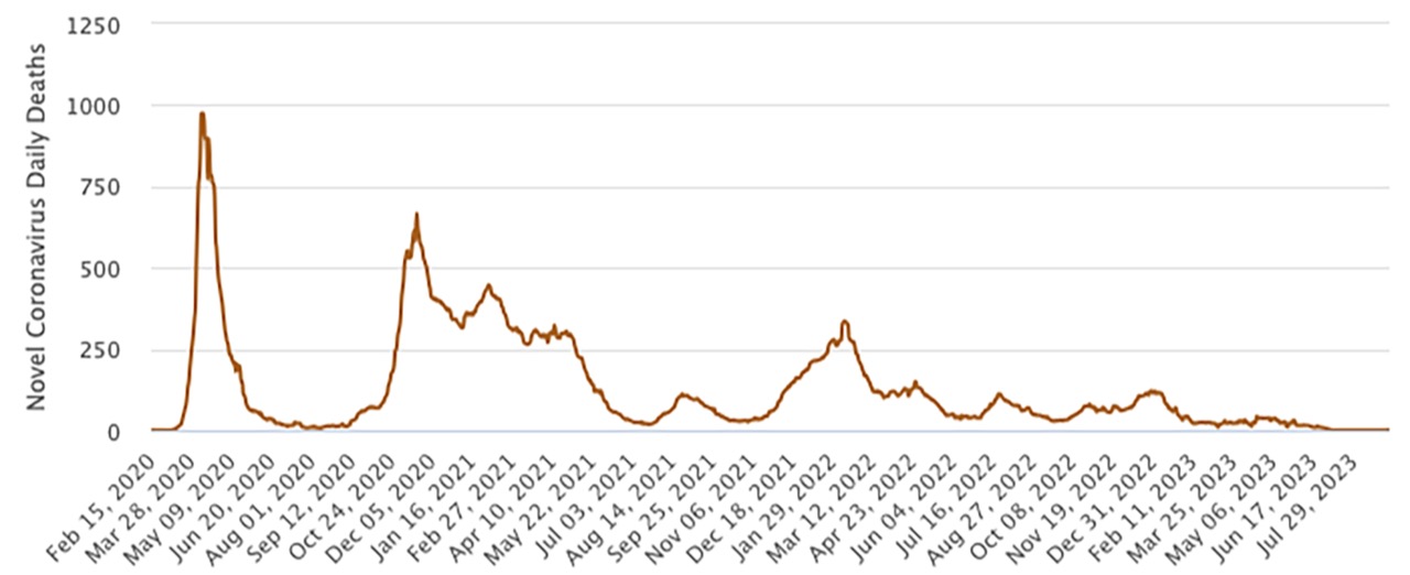
Figure 1: The reported time dependences of the daily Covid death rates (7-day moving average) for the (a) USA, (b) UK, (c) Brazil, (d) Italy, (e) Russia, and (f) France. These data cover the period from Feb. 15 2020 until July 29, 2023 and are all taken from Ref. Cov (2023).

To illustrate these statements, Fig. 1 plots the reported daily death rates for the six countries in the world with populations greater than 60 million and with the largest total death rates. They are: USA (3.507 deaths/1000), UK (3.339/1000), Brazil (3.275/1000), Italy (3.174/1000), Russia (2.743/1000), and France (2.556/1000). For reference, the country with the largest reported total death rate is Peru (6.582/1000), while the world average is (0.887/1000). For many reasons, the accuracy of the data may vary widely from country to country so that some of the numbers reported in Ref. Cov (2023), such as the suspicious smoothness of the data for Russia, should be interpreted with caution.

One of the many confounding features of Covid-19 is asymptomatic transmission, in which the epidemic may be unknowingly spread by individuals who did not know that they were contagious. Partly because of this feature, a wide variety of increasingly sophisticated multi-compartment models were developed that build on the classic SIR and SIS models of epidemic spread. These models typically attempted to faithfully account for subpopulations in various stages of the disease and recovery, as well as the transitions between these stages. Models of this type gave rise to complex dynamical behaviors that could sometimes mirror reality in a specific setting or over a limited time range. However, embellishments of SIR and SIS-type models still seem to be incomplete because of the difficulty in simultaneously accounting for both the disease dynamics and its interaction with social forces.

The discrepancy between the observed wildly varying features of Covid-19 and supposedly deterministic outcomes of SIR and SIS models is especially striking. In fact the determinism of the SIR and SIS models is actually illusory. The SIR model, for example, is an inherently stochastic process Bailey (1950, 1987) that is characterized by the reproductive number $R_{0}$. This quantity is defined as the average number of individuals to whom a single infected individual transmits the infection before this single individual recovers. In the supercritical regime, $R_{0}>1$, it is possible that the outbreak may quickly die out. This happy event occurs with probability $R_{0}^{-1}$ if one individual was initially infected. Otherwise, the infection quickly spreads, and the behavior becomes effectively deterministic. Namely a finite fraction $c=c(R_{0})$ individuals catch the disease, with $c$ implicitly determined by the criterion Hethcote (2000)

$$c+e^{-cR_{0}}=1$$ (1)

Conversely, if $R_{0}<1$, the outbreak quickly dies out, so while the subcritical SIR process is still manifestly stochastic, it is not a threat to the population at large. The interesting and the most strongly stochastic behavior emerges in critical SIR and SIS models Ridler-Rowe (1967); Grassberger (1983); Martin-Löf (1998); Ben-Naim and Krapivsky (2004); Kessler and Shnerb (2007); Kessler (2008); Gordillo et al. (2008); Greenwood and Gordillo (2009); Van der Hofstad et al. (2010); Antal and Krapivsky (2012); Ben-Naim and Krapivsky (2012); Krapivsky (2021). For the SIR mode, in particular, the distribution of the number of infected individuals has a power-law tail. For a finite population of size $N$ the critical SIR model does not lead to a pandemic, because the average number of individuals who contract the disease scales as $N^{1/3}$.

Here we argue that significant forecasting uncertainties are an integral feature of processes caused by the interplay between the dynamics of the disease transmission and the social forces that arise in response to the epidemic. Each attribute alone typically leads to either exponential growth (due to disease transmission at early times) or to exponential decay (due to effective mitigation strategies). Within our model, the competition between these two exponential processes leads to a dynamics that is extremely sensitive to seemingly minor details. The basic mechanism in our modeling is that the reproductive number $R_{0}$ can sometimes decrease, due to the imposition of public-health measures, such as social distancing, vaccinations, etc., and sometimes increase, because of the relaxation of these measures. Focusing only on the dynamics of the reproductive number serves as a useful proxy for the myriad of influences that control the true epidemic dynamics. Within this framework, we will determine the duration of an epidemic, the time dependence of the number of infected individuals, and the total number of individuals infected when an epidemic finally ends. All three quantities exhibit huge fluctuations that are reminiscent of the actual data.

II Systematic Mitigation

As a preliminary, we first investigate what we term as the systematic mitigation strategy. Here increasingly stringent controls are imposed as soon as an outbreak is detected until the reproductive number $R_{0}$ is reduced to below 1. Once $R_{0}<1$, progressively fewer individuals are infected after each incubation period, so that the epidemic soon disappears. The condition $R_{0}=1$ defines the end of the epidemic. Because society is a complicated, with many competing social forces in play, we posit that it is not possible to reduce $R_{0}$ instantaneously, but rather, the reduction happens gradually. We therefore assume that after each successive incubation period $R_{0}$ is decreased by a random number $r$ whose average value $\langle r\rangle$ is less than 1. While additional individuals will become infected after $R_{0}$ has been reduced to less than 1, their number decays exponentially with time and constitute a negligible contribution to the total number of infections.

Define $R_{k}$ as the reproductive number on the $k^{\rm th}$ period. Then $R_{k}$ is given by

$$R_{k}=r_{k}\,R_{k-1}=r_{k}\,r_{k-1}\ldots r_{2}\,r_{1}\,R_{0}\,,$$ (2)

where $r_{k}$ is the value of the random variable $r$ in the $k^{\rm th}$ period. The typical number of periods $k$ until $R_{0}$ reaches 1 is determined by $R_{0}\,\langle r\rangle^{k}=1$. In what follows, we assume that when the epidemic is first detected, the reproductive number $R_{0}=2.5$, and we take $\langle r\rangle=0.95$ for illustration. With these conventions,

$$k=\frac{\ln(1/R_{0})}{\ln\langle r\rangle}=\frac{\ln(1/2.5)}{\ln(0.95)}\approx 17.86$$

Thus the epidemic typically disappears after 18 periods. However, because of the inherent randomness in the mitigation, with $R_{0}$ sometimes decreasing by less than 0.95 and sometimes by more than 0.95, the true epidemic dynamics can be very different, as illustrated in Fig. 2.

  

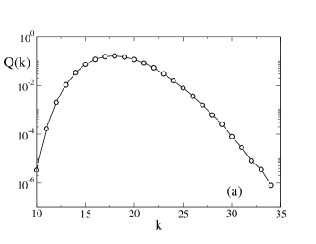
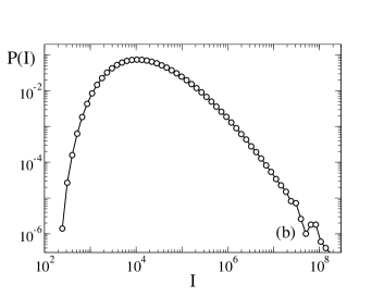
Figure 2: Systematic mitigation: (a) The probability $Q(k)$ that the epidemic lasts $k$ periods. (b) The probability $P(I)$ that the epidemic has ultimately infected $I$ people (under the assumption that the initial epidemic size is one person).

We simulate the systematic mitigation strategy by starting with a single infected individual and reproductive number $R_{0}=2.5$. We then choose a set of random numbers $r_{1},r_{2},r_{3},\ldots$, each of which are uniformly distributed between 0.9 and 1, so that $\langle r\rangle=0.95$. We first measure how long it takes until $R_{k}$, the reproductive number in the $k^{\rm th}$ period, is reduced to 1, which signals the end of the epidemic. We perform this same measurement for $5\times 10^{6}$ different choices of the set of random numbers $r_{1},r_{2},\ldots,r_{k}$. As shown in Fig. 2(a), the probability $Q(k)$ that the epidemic is extinguished in $k$ periods is peaked at roughly 18 periods, consistent with the naive estimate above. If one is lucky, that is, if most of the reduction factors $r_{i}$ are close to 0.9, the epidemic can be extinguished in as little as 11 periods. If one is unlucky (many of the $r_{i}$ are close to 1), the epidemic can last more than 30 periods.

While the distribution of epidemic durations is fairly narrow, the size of an epidemic, namely, the total number $I$ of people who were infected during the course of an epidemic,

$$I=R_{0}+R_{1}+R_{2}+\ldots+R_{k}\,,$$ (3)

can vary by several orders of magnitude. It is important to point out that the number of newly infected people is based on the assumption that this number is small compared to the total population size, so that the growth in the number of new infections is truly exponential. As shown in Fig. 2(b), while the most probable epidemic size is $\approx 10^{4}$ (again starting with a single infected individual), there is a non-vanishing probability that the outbreak size can be as small as a few thousand or greater than $10^{7}$. This large disparity in outbreak sizes illustrates how small changes in the way that the epidemic is mitigated can lead to huge changes in the outbreak size.

More dramatically, suppose that the mitigation strategy is slightly less effective and that the reproductive number is reduced at each period by a uniform random variable that lies between $[0.95,1]$ rather than between $[0.9,1]$. Now the epidemic can last between 22 and 55 periods, with a most probable duration of 36 periods. However, the epidemic size ranges between roughly $10^{5}$ and $10^{12}$, with a most probable size of roughly $7\times 10^{7}$. The upper value is much larger than the world population and the finiteness of the population would now provide the upper bound. Although this second epidemic lasts twice as long as the first one, it typically infects 7,000 times more people! We emphasize that the stochastic nature of the random variables $r_{j}$ plays a decisive role. Very different behaviors emerge in the deterministic case Bianconi and Krapivsky (2020).

We also mention that the systematic mitigation strategy is analytically tractable because of a close relation between the epidemic size in (3) and Kesten variables Kesten (1973), which appear in probability theory, one-dimensional disordered systems, and various other subjects. We explain this connection in Appendix A and also several analytical results that qualitatively agree with our numerical observations. As one example, we show that the slightly faster than exponential decay of $P(I)$ suggested by Fig. 2 may be close to a factorial decay.

III Vacillating Mitigation

During the acute period of the pandemic in 2020–2021, there was considerable and even vitriolic debate about the efficacy of various mitigation strategies, or even about the utility of any mitigation. If the epidemic is severe, as quantified by the reproductive number $R_{k}$ in the $k^{\rm th}$ period being substantially greater than 1, people may be more likely to accept restrictions on their behaviors, such as isolating, masking, vaccinating, etc., to reduce their risk of getting sick. These adaptations will reduce the reproductive number. If, however, the reproductive number becomes less than 1, then people will want to relax their vigilance and may also advocate for the opening of various public venues, such as schools, theaters, stadiums, etc. We model this tug-of-war between increased and decreased restrictions by what we term as the vacillating mitigation strategy. This perspective of treating the competition between epidemiology and social behavior was previously treated in more sophisticated models Manrubia and Zanette (2022); Tkachenko et al. (2021). We emphasize that our model merely a proxy for the two competing influences of epidemiology and social behavior.

The two competing steps of the vacillating strategy are the following:

• Mitigation: if $R_{k}>1$, decrease $R_{k}$ by a factor $r$ that is uniformly distributed in $[a,1]$, with $a<1$.

• Relaxation: if $R_{k}<1$, change $R_{k}$ by a factor $s$ that is uniformly distributed in $[a,3-2a]$.

The first option is the same as in the systematic mitigation strategy. We construct the second option by requiring that $\langle s\rangle=1+\frac{1}{2}(1-a)$ and $\langle r\rangle=1-\frac{1}{2}(1-a)$ are symmetrically located about 1. That is, the average decrease in $R_{k}$ in a mitigation step equals the average increase in $R_{k}$ in the relaxation step. This symmetrical construction seems appropriate to probe the long-term influence of vacillation on the dynamics. If the vacillation strategy was biased towards relaxation, $R_{0}$ would remain greater than 1 and the entire planet would be infected. If this strategy was biased towards mitigation, the epidemic would be similar to that in systematic mitigation. Neither of these cases is interesting from the viewpoint of probing long-time behaviors.

  

  

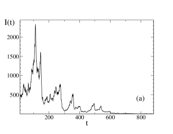
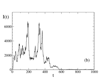
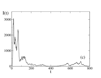
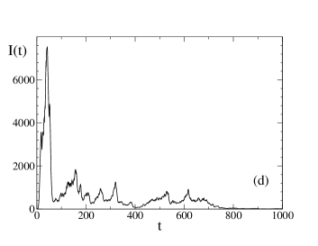
Figure 3: Representative trajectories for the number of people $I(t)$ infected at time $t$ for the vacillating mitigation strategy when starting with $R_{0}=1$ and a single infected person.

In this vacillating strategy, $R_{k}$ varies between values greater than 1 and values less than 1. This would lead to an eternal epidemic. To avoid this unrealistic outcome, the other important feature of the relaxation step is that the value of $R_{k}$ could still decrease during a relaxation step because $a<1$. This possibility ensures that eventually less than one person will be infected in the current incubation period. We now define this event as signaling the end of the epidemic.

Figure 3 shows a few representative trajectories of the number of people infected $I(t)$ as a function of time (incubation periods) from the same initial condition of a single infected person and $R_{0}=2.5$. While there are some qualitative differences between the trajectories of Fig. 1 and the model outcomes, the important points that are common to the real data and the simulation results are the disparities in the individual trajectories and the strongly fluctuating temporal behavior.

    

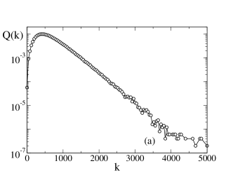
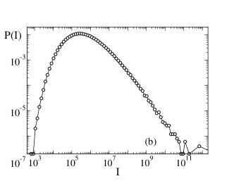
Figure 4: Vacillating mitigation: (a) The probability $Q(k)$ that the epidemic lasts $k$ periods. (b) The probability $P(s)$ that the epidemic has ultimately infected $s$ people (under the assumption that the initial epidemic size is one person).

For the vacillating strategy and for the choice $a=0.9$, the most likely duration of the epidemic is roughly 400 periods (Fig. 4(a)), compared to 18 periods for the systematic strategy. The probability that the epidemic lasts much longer than the most likely value decays exponentially with time. An even more dramatic feature of the vacillating strategy is the number of people that are ultimately infected. The most probable outcome is that $3\times 10^{5}$ people are infected when the epidemic ends (Fig. 4(b)). However, the typical size of the epidemic can range from $10^{4}$ to $10^{8}$. Compared to the systematic mitigation strategy with a reduction factor uniformly in the range $[0.9,1]$, the epidemic now lasts roughly 20 times longer and infects a factor 30 more individuals.

IV Concluding Remarks

This work should not be construed to mean that public-health measures should be ignored. Indeed, the extremely rapid development of a vaccine that is effective against Covid-19 is an outstanding triumph of modern medical science. It should also be pointing out that some of the many forecasting models for Covid-19 were useful during the early stages of the pandemic. However, when social influences with competing viewpoints began to dictate individual and collective policy decisions, much of the predictive power of forecasting models was lost.

We also emphasize that our simplistic model has little connection to the actual epidemiological and social processes that determine the spread of the epidemic and the changes in individual and collective behaviors in response to the epidemic. Nevertheless, our model seems to capture the tug of war between public-health mandates to control the spread of the disease and the social forces that often advocate for a more laissez-faire approach. Our main message is that there are huge uncertainties in predicting the time course of an epidemic, its ultimate duration, and the final outbreak size. This unpredictability seems to be intrinsic to the dynamics of epidemics where epidemiological influences occur in concert with social forces. In this setting, forecasting ambiguity is unavoidable.

We thank J. M. Luck for helpful correspondence. This research was partially supported by NSF grant DMR-1910736.

Appendix A Kesten variables

We outline an analytical treatment of the systematic mitigation strategy. Since the terms in the sum in Eq. (3) decay exponentially in the number of factors in the product, we can replace the finite sum in (3) by the infinite sum

$$R=1+r_{1}+r_{1}r_{2}+r_{1}r_{2}r_{3}+\ldots,\qquad R=I/R_{0}\,,$$ (4)

because it changes the outcome just by a finite number. Random variables that are defined by (4) are known Kesten variables, which have fundamental implications Kesten (1973); Solomon (1975); Vervaat (2010) and a variety of applications Derrida and Hilhorst (1983); de Calan et al. (1985); Luck and Nieuwenhuizen (1988); Nieuwenhuizen and van Rossum (1991); Buraczewski et al. (2013); Gautié et al. (2021); Gueneau et al. (2023).

We now show how to probe the probability distribution $P(R)$ using Kesten variables. The definition of Kesten variables implies that $P(R)$ satisfies the integral equation

$$P(R)=\int dr\,\rho(r)\int dQ\,P(Q)\,\delta[R-1-rQ]\,.$$ (5)

By performing the Laplace transform

$$\widehat{P}(s)=\int_{1}^{\infty}dR\,P(R)\,e^{-sR}\,,$$ (6)

the Laplace transform of the probability distribution $P(R)$ can be expressed as

$$\widehat{P}(s)=\int_{1}^{\infty}dQ\,P(Q)\int dr\,\rho(r)\,e^{-s-srQ}\,.$$ (7)

As a simple example, let us treat the uniform distribution, $\rho(r)=1$ when $r\in[0,1]$. Then Eq. (7) becomes

$$s\,e^{s}\widehat{P}(s)=\int_{1}^{\infty}dQ\,P(Q)\,\frac{1-e^{-sQ}}{Q}\,.$$ (8)

Differentiating with respect to $s$ we obtain

$$\frac{d\Pi(s)}{ds}=s^{-1}e^{-s}\,\Pi(s),\qquad\Pi(s)=s\,e^{s}\,\widehat{P}(s)\,,$$ (9)

whose solution is

$$\widehat{P}(s)=|s|^{-1}\exp[-s-\gamma+\text{Ei}(-s)]\,,$$ (10)

where $\gamma=0.577\,215\ldots$ is the Euler constant and $\text{Ei}(\cdot)$ is the exponential integral.

Because this Laplace transform exists for all $s\in\mathbb{R}$, $P(R)$ decays faster than exponentially in $R$ for $R\to\infty$; this bound ensures that the Laplace transform (6) remains well-defined when $s\to-\infty$. Using (10) we find

$$\ln\widehat{P}(-\sigma)=\text{Ei}(\sigma)+\sigma-\ln\sigma-\gamma\,,$$ (11)

which grows as $\sigma^{-1}e^{\sigma}$ when $\sigma\gg 1$. This limiting behavior leads to

$$\ln P(R)\simeq-R\,\ln R$$ (12)

for $R\gg 1$. This is essentially a factorial decay: $P(R)\propto 1/\Gamma(R)$, where $\Gamma(\cdot)$ is the Euler gamma function. This behavior is consistent with the faster than exponential decay of $P(R)$ observed in simulations (Fig. 2(b)). For the small-$R$ behavior, we use the asymptotic $\widehat{P}(s)\simeq s^{-1}\exp[-s-\gamma]$ as $s\gg 1$ to give $P(1)=e^{-\gamma}=0.561\,459\ldots$. This disagrees with simulations (see Fig. 2(b)), where $\rho(r)$ was chosen from a uniform distribution in $[a,1]$, with $a=0.9$. The reason for this discrepancy is simple: when $\rho(r)$ vanishes for $r<a$, it is very unlikely to generate a value of $R$ that is close to the minimum value $R_{\text{min}}=(1-a)^{-1}$ because it requires each $r_{i}$ to be close to $a$.

If the support $[a,b]$ of the distribution $\rho(r)$ is not inside $[0,1]$, that is, $b>1$, the Kesten variable still has a stationary distribution if

$$\int_{a}^{b}dr\,\rho(r)\ln r<0$$ (13)

Here, the large-$R$ behavior of $P(R)$ is again algebraic Kesten (1973), $P(R)\sim R^{-\beta}$, where $\beta$ is the smallest root of the equation $\int_{a}^{b}dr\,\rho(r)r^{\beta-1}=1$ that also satisfies $\beta>1$. For example, for an arbitrary distribution with support that is symmetric about $r=1$ (so that it satisfies $\rho(r)=\rho(2-r)$), the requirement (13) is always obeyed, so the Kesten variable is stationary. Here the decay exponent is universal: $\beta=2$. Thus, already the first moment $\int dR\,RP(R)$ diverges.

Mitigation strategies are necessarily successful when $\rho(r)$ has its support inside $[0,1]$. For distributions $\rho(r)$ defined in $[a,b]$ with $b>1$, even if the stationarity requirement (13) is obeyed, the distribution for for the outbreak size $P(R)$ has an algebraic tail, which implies that a finite fraction of population contracted the disease. While the emergence of these heavy-tailed distributions sparked interest Kesten (1973); Solomon (1975); Vervaat (2010); Derrida and Hilhorst (1983); de Calan et al. (1985); Luck and Nieuwenhuizen (1988); Nieuwenhuizen and van Rossum (1991) in Kesten variables, in the context of pandemics, such a feature is to be avoided.

References

- Cov (2023) “Covid-19 coronavirus pandemic,” https://www.worldometers.info/coronavirus (2023).
- Bailey (1950) N. T. J. Bailey, “A simple stochastic epidemic,” Biometrika 37, 193–202 (1950).
- Bailey (1987) N. T. J. Bailey, The Mathematical Theory of Infectious Diseases (Oxford University Press, Oxford, 1987).
- Hethcote (2000) H. W. Hethcote, “The mathematics of infectious diseases,” SIAM Rev. 42, 599–653 (2000).
- Ridler-Rowe (1967) C. Ridler-Rowe, “On a stochastic model of an epidemic,” J. Appl. Prob. 4, 19–33 (1967).
- Grassberger (1983) P. Grassberger, “On the critical behavior of the general epidemic process and dynamical percolation,” Math. Biosciences 63, 157–172 (1983).
- Martin-Löf (1998) A. Martin-Löf, “The final size of a nearly critical epidemic, and the first passage time of a Wiener process to a parabolic barrier,” J. Appl. Probab. 35, 671–682 (1998).
- Ben-Naim and Krapivsky (2004) E. Ben-Naim and P. L. Krapivsky, “Size of outbreaks near the epidemic threshold,” Phys. Rev. E 69, 050901 (2004).
- Kessler and Shnerb (2007) D. A. Kessler and N. M. Shnerb, “Solution of an infection model near threshold,” Phys. Rev. E 76, 010901 (2007).
- Kessler (2008) D. A. Kessler, “Epidemic size in the SIS model of endemic infections,” J. Appl. Probab. 45, 757–778 (2008).
- Gordillo et al. (2008) L. F. Gordillo, S. A. Marion, A. Martin-Löf, and P. E. Greenwood, “Bimodal epidemic size distributions for near-critical SIR with vaccination,” Bull. Math. Biol. 70, 589–602 (2008).
- Greenwood and Gordillo (2009) P. E. Greenwood and L. F. Gordillo, “Stochastic epidemic modeling,” in Mathematical and Statistical Estimation Approaches in Epidemiology, edited by G. Chowell, J. M. Hyman, L. M. A. Bettencourt, and C. Castillo-Chavez (Springer Netherlands, Dordrecht, 2009) pp. 31–52.
- Van der Hofstad et al. (2010) R. Van der Hofstad, A. Janssen, and J. Van Leeuwaarden, “Critical epidemics, random graphs, and Brownian motion with a parabolic drift,” Adv. Appl. Probab. 42, 1187–1206 (2010).
- Antal and Krapivsky (2012) T. Antal and P. L. Krapivsky, “Outbreak size distributions in epidemics with multiple stages,” J. Stat. Mech. 2012, P07018 (2012).
- Ben-Naim and Krapivsky (2012) E. Ben-Naim and P. L. Krapivsky, “Scaling behavior of threshold epidemics,” Eur. Phys. J. B 85, 145 (2012).
- Krapivsky (2021) P. L. Krapivsky, “Infection process near criticality: influence of the initial condition,” J. Stat. Mech. 2021, 013501 (2021).
- Bianconi and Krapivsky (2020) G. Bianconi and P. L. Krapivsky, “Epidemics with containment measures,” Phys. Rev. E 102, 032305 (2020).
- Kesten (1973) H. Kesten, “Random difference equations and Renewal theory for products of random matrices,” Acta Math. 131, 207–248 (1973).
- Manrubia and Zanette (2022) S. Manrubia and D. H. Zanette, “Individual risk-aversion responses tune epidemics to critical transmissibility (R=1),” Royal Society Open Science 9, 211667 (2022).
- Tkachenko et al. (2021) A. V. Tkachenko, S. Maslov, T. Wang, A. Elbana, G. N. Wong, and N. Goldenfeld, “Stochastic social behavior coupled to Covid-19 dynamics leads to waves, plateaus, and an endemic state,” Elife 10, e68341 (2021).
- Solomon (1975) F. Solomon, “Random walks in a random environment,” Ann. Probab. 3, 1–31 (1975).
- Vervaat (2010) W. Vervaat, “On a stochastic difference equation and a representation of non-negative infinitely divisible random variables,” Adv. Appl. Probab. 11, 750–783 (2010).
- Derrida and Hilhorst (1983) B. Derrida and H. J. Hilhorst, “Singular behaviour of certain infinite products of random matrices,” J. Phys. A 16, 2641 (1983).
- de Calan et al. (1985) C. de Calan, J. M. Luck, Th. M. Nieuwenhuizen, and D Petritis, “On the distribution of a random variable occurring in 1D disordered systems,” J. Phys. A 18, 501–523 (1985).
- Luck and Nieuwenhuizen (1988) J. M. Luck and Th. M. Nieuwenhuizen, “Lifshitz tails and long-time decay in random systems with arbitrary disorder,” J. Stat. Phys. 52, 1–22 (1988).
- Nieuwenhuizen and van Rossum (1991) Th. M. Nieuwenhuizen and M. C. W. van Rossum, “Universal fluctuations in a simple disordered system,” Phys. Lett. A 160, 461–464 (1991).
- Buraczewski et al. (2013) D. Buraczewski, E. Damek, T. Mikosch, and J. Zienkiewicz, “Large deviations for solutions to stochastic recurrence equations under Kesten’s condition,” Ann. Probab. 41, 2755–2790 (2013).
- Gautié et al. (2021) T. Gautié, J.-P. Bouchaud, and P. Le Doussal, “Matrix Kesten recursion, inverse-Wishart ensemble and fermions in a Morse potential,” J. Phys. A 54, 255201 (2021).
- Gueneau et al. (2023) M. Gueneau, S. N. Majumdar, and G. Schehr, “Active particle in a harmonic trap driven by a resetting noise: an approach via Kesten variables,” arXiv:2306.09453 (2023).