Gaining Insights into Denoising by Inpainting

Abstract

The filling-in effect of diffusion processes is a powerful tool for various image analysis tasks such as inpainting-based compression and dense optic flow computation. For noisy data, an interesting side effect occurs: The interpolated data have higher confidence, since they average information from many noisy sources. This observation forms the basis of our denoising by inpainting (DbI) framework. It averages multiple inpainting results from different noisy subsets. Our goal is to obtain fundamental insights into key properties of DbI and its connections to existing methods. Like in inpainting-based image compression, we choose homogeneous diffusion as a very simple inpainting operator that performs well for highly optimized data. We propose several strategies to choose the location of the selected pixels. Moreover, to improve the global approximation quality further, we also allow to change the function values of the noisy pixels. In contrast to traditional denoising methods that adapt the operator to the data, our approach adapts the data to the operator. Experimentally we show that replacing homogeneous diffusion inpainting by biharmonic inpainting does not improve the reconstruction quality. This again emphasizes the importance of data adaptivity over operator adaptivity. On the foundational side, we establish deterministic and probabilistic theories with convergence estimates. In the non-adaptive 1-D case, we derive equivalence results between DbI on shifted regular grids and classical homogeneous diffusion filtering via an explicit relation between the density and the diffusion time.

65D18, 68U10, 94A08

1 Introduction

One of the most fascinating properties of certain variational models in image analysis is their filling-in effect: The smoothness term (regularizer) inserts information at locations where the data term is absent or small in magnitude. This is a key concept to create powerful models for image inpainting and optic flow computation. The gradient flow for minimizing the variational energy functional leads to partial differential equations (PDEs) with a diffusion term. In our paper, we are particularly interested in an unconventional application of diffusion-based inpainting models, where we explore their filling-in effect for the purpose of denoising.

Image inpainting is the task of reconstructing missing parts of an image from only a subset of known image data [10, 31, 39, 63, 76]. When this subset – the so-called mask – is a scattered set of pixels, the inpainting is termed sparse inpainting. The filling-in effect of diffusion processes can be applied to image inpainting problems by setting the known data as boundary values for the diffusion equation. Sophisticated nonlinear diffusion processes can achieve remarkable reconstruction quality for sparse inpainting, enabling efficient lossy image codecs [37, 50, 75] competitive to JPEG [66] and JPEG2000 [79]. Surprisingly, already the simplest linear diffusion method – homogeneous diffusion [46] – can produce excellent, structure-preserving sparse inpainting results, as long as the location and values of the known pixels are optimized carefully [8, 12, 13, 22, 41, 61]. Especially on piecewise constant images, such as cartoon images, depth maps or flow fields, homogeneous diffusion inpainting in conjunction with edge or segment information performs very well [17, 38, 43, 48, 49, 59, 60]. This even allows some of these methods [48, 49] to outperform HEVC [77] on such data.

If diffusion-based inpainting is performed on noisy data, the noisy mask pixels remain unchanged during the process, while the unknown areas in between are interpolated smoothly by averaging information from the noisy pixels. We thus have a scenario, where the inpainted data can be more reliable than the known data – an observation that may appear paradoxical at first glance. For variational optic flow estimation [45, 64, 83] a similar effect occurs: In [14], the authors show that the parts of the flow field that are filled in by the diffusion-like regularization terms are usually the ones with the highest confidence. These considerations, which we visualize in Figure 1, suggest to study this filling-in effect for the denoising of images and to pursue the unconventional idea of denoising by inpainting.

(a) original	(b) noisy	(c) mask	(d) inpainting
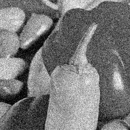
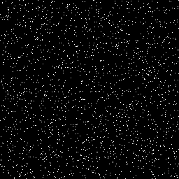
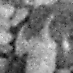
peppers	$\sigma_{n}=30$	$3\%$ density	HD inpainting

Figure 1: Homogeneous diffusion (HD) inpainting on the test image peppers ($256\times 256$ pixels, image range $[0,255]$) with additive Gaussian noise of standard deviation $\sigma_{n}=30$ that we do not clip. The mask pixels are randomly selected. Note that the inpainted pixels are more reliable, since they average noisy information from the neighborhood. This filling-in effect is the motivation for denoising by inpainting. The visual difference is also reflected by the mean squared error (MSE): The MSE of the noisy image in (b) is 904. Since the mask pixels are chosen randomly and are not changed by the inpainting, the MSE at mask pixel locations in (d) is still approximately 900. However, the total image MSE in (d) is only 475.

1.1 Our Contribution

The goal of our work is to shed some light on the connections between PDE-based inpainting and denoising, two tasks which have coexisted for a long time, while their links have hardly been studied so far. We aim to close this gap by investigating the denoising potential of sparse inpainting. Our intention is not to achieve state-of-the-art denoising performance, but rather to gain valuable theoretical and algorithmic insights. For surveys on highest quality denoising methods, we refer to [33, 58]. We focus on homogeneous diffusion, since this process is widely used in inpainting-based compression and is particularly simple, such that a rigorous theoretical analysis is possible. Since denoising methods can also be used as Plug-and-Play priors in algorithms for solving inverse problems [57, 73, 80], our relations between inpainting and denoising approaches may have an even broader application spectrum.

The present paper builds upon our previous conference publication [1], in which the basic denoising by inpainting framework is presented. This framework reconstructs a denoised version of an image by averaging the results of multiple inpaintings obtained from distinct masks. Furthermore, two concrete implementations of this framework are proposed in [1]: The first uses shifted regular masks and allows to establish a relation between denoising by inpainting and classical diffusion filtering in 1D, while the second uses probabilistic densification to adapt the masks to the image structures and enables an edge-preserving denoising behavior. We extend the aforementioned results by providing a broad study that includes a theory and practical improvements of the framework in [1]:

• We provide deterministic and probabilistic theories for the DbI framework that has only been heuristically motivated so far [1]. This allows us to better explain the observed denoising performance of the framework and to formulate a convergence rate for the proposed methods.

• For regular masks in 1D, we prove a general relation between the mask density and the diffusion time. We also propose a generalization of this result to 2D for uniform random masks.

• We add an additional step that optimizes the gray values at mask pixels (tonal optimization) to the denoising by inpainting framework [1]. We examine its interplay with different mask selection strategies and gain insights about the potential of tonal optimization in the noisy setting.

• We devise a practical adaptive mask selection method for denoising by inpainting. It exploits the newly added tonal optimization step and is orders of magnitude faster than the one presented in [1], while even outperforming it in terms of denoising quality.

• We extend the DbI framework to a higher-order linear inpainting operator – biharmonic inpainting – and show that for optimized data, this more complex operator does not yield better quality. This justifies our shift in focus from operator optimization to data optimization.

1.2 Related Work

Since we use inpainting methods for image denoising, we give an overview of some relevant methods from both fields and relate them to our work. This also elucidates the close connection between the two tasks.

PDE-based Denoising and Inpainting

Our proposed methods borrow several ideas from sparse PDE-based inpainting methods [37] that are useful e.g., for inpainting-based compression. We mostly restrict ourselves to homogeneous diffusion inpainting [17], which can be implemented very efficiently [5, 23, 44, 51, 52, 60], and – in spite of its simplicity – can produce convincing results for suitably chosen data [8, 12, 22, 41, 42, 61, 65]. Nonlinear diffusion inpainting methods, e.g., edge-enhancing diffusion (EED) inpainting [37, 84], can improve reconstruction quality but are more complex due to their nonlinearity. This complexity also carries over to the data optimization process. Higher-order inpainting operators can also be used for sparse inpainting [16, 22, 37, 75, 78], but can be more sensitive to noise. The quality of PDE-based sparse inpainting approaches strongly depends on mask optimization, and in our denoising by inpainting framework we rely heavily on spatial optimization [8, 12, 22, 23, 41, 42, 60, 61, 65] and tonal optimization [22, 23, 42, 61, 68].

For fairness reasons, we compare the quality of our proposed method to classical diffusion-based image denoising methods, namely homogeneous diffusion [46], linear space-variant diffusion [36] as well as nonlinear diffusion [66]. We choose these methods because they are closest conceptually so we expect useful insights about our method. Furthermore, we compare to total variation (TV) regularization [74], which is a classical PDE-based denoising method that has also been used for image inpainting [19].

Patch-based Denoising and Inpainting

Aside from PDE-based approaches, there exist other classes of methods for inpainting, one of them being patch- or exemplar-based methods. These methods work especially well with textured data. The idea is to copy similar patches from known to unknown regions. Efros and Leung have proposed the first exemplar-based inpainting method [31], but many versions have been developed since then (e.g., [2, 6, 7, 27]), including the method of Facciolo et al. for sparse inpainting [34]. Inpainting approaches combining PDE-based and patch-based methods have also been presented [11, 70].

Inspired by the method of Efros and Leung [31], a patch-based denoising method called NL-means [15] has been proposed. It denoises an image based on a nonlocal weighted averaging of similar image patches. Other algorithms such as the famous BM3D algorithm [28] are also based on the filtering of image patches. These observations further substantiate the ties between denoising and inpainting. The NL-means method can even be interpreted as a case of a denoising by inpainting approach, although it does not use the inpainting ideas as directly as we do. Of course, a direct application of patch-based inpainting techniques would lead to the copying of erroneous noisy data, and not to a denoising effect. Since adapting patch-based inpainting methods to denoising appears to be highly nontrivial, we restrict ourselves only to diffusion-based approaches in this work.

Sparse Signal Approximation

Another popular approach in the field of image denoising relies on the idea that signals (and images) can be represented as a linear combination of a smaller number of basis signals, that are selected from a so-called dictionary [32]. This is often done by applying a transform which can be implemented efficiently (e.g., a wavelet transform [62] or a discrete cosine transform (DCT) [3]), that makes the signal representation sparse. In these cases, the dictionary is the set of basis vectors of the transformed domain. Small coefficients are ignored as they are assumed to be induced by the noise, and the image is represented only by the basis vectors corresponding to larger coefficients. The famous wavelet shrinkage algorithm [30] is an example of such an approach. Starting with a shift-invariant wavelet transform [25], a number of overcomplete dictionaries have been proposed in the literature. It has been demonstrated that redundancy introduced through an overcomplete basis can improve denoising performance over orthogonal transforms [71].

To fill in missing information in images, several authors also consider sparse representations in some transform domain such as the DCT [40] or the shearlet domain [54]. This shows another bridge between the two tasks of denoising and inpainting. Hoffmann et al. [44] relate linear PDE-based inpainting methods to concepts from sparse signal approximation. They solve the inpainting problem with the help of discrete Green’s functions [9, 24], which can be interpreted as atoms in a dictionary. This allows for a sparse representation of the inpainting solution. Kalmoun et al. [51] follow a similar approach by solving homogeneous diffusion inpainting with the charge simulation method [53, 56]. An application of homogeneous diffusion inpainting with Green’s functions is the video codec by Andris et al. [5].

We justify certain design choices of our proposed method with results from this field. Specifically, our approach also exploits the redundancy introduced by overcomplete bases.

Cross-Validation

We also see the work of Craven and Wahba [26] on (generalized) cross-validation as conceptually related to parts of our work. Cross-validation can be used to optimize parameters in denoising models [26, 86]. It removes data points from given noisy observations and judges the quality of a parameter selection in terms of the model’s capability to reconstruct the data at these locations. Related ideas are also pursued in [18]. Probabilistic densification [43] and sparsification [61], two concepts from spatial optimization that we consider in our framework, also use the error of the inpainted reconstruction at left out locations – in our case also on noisy data. Yet, both applications differ, as the goal of the latter methods is to construct an inpainting mask and not to optimize model parameters.

Neural Denoising and Inpainting

In recent years, many very powerful methods for inpainting and denoising have been proposed that rely on neural networks. They are, however, not a topic of our paper, since we aim at gaining structural insights into the connections between inpainting and denoising. This requires simple and transparent models. It is our hope that in the long run, our insights can also be generalized to neural approaches.

1.3 Paper Organization

In Section 2 we briefly introduce the basic idea behind diffusion filtering and its application to image denoising and image inpainting. In Section 3 we present the general framework for denoising by inpainting from [1] and provide a deterministic and probabilistic theory for it, along with an interpretation of its potential performance. In Section 4 we devise different mask optimization strategies following ideas from image compression and adapt them such that they fit the task of denoising by inpainting. Our experiments and results are presented in Section 5, and we conclude the paper in Section 6.

2 Basics of Diffusion Filtering

In its original context of physics, diffusion is a process that equilibrates particle concentrations. When working with images, we interpret the gray values as particle concentrations and use diffusion processes as smoothing filters that balance gray value differences. To this end, we define the original grayscale image as a function $f:\Omega\to\mathbb{R}$, with $\Omega\subset\mathbb{R}^{2}$ being a rectangular image domain. Similarly, $u:\Omega\times[0,\infty)\to\mathbb{R}$ denotes the evolving, filtered image. Then the diffusion evolution is described by the following PDE:

(1) $$\partial_{t}u(\bm{x},t)=\operatorname{div}(g\bm{\nabla}u(\bm{x},t))\quad\textnormal{for }\bm{x}\in\Omega,\,\,t\in(0,\infty).$$

Here $t$ denotes time, $\bm{\nabla}=(\partial_{x},\partial_{y})^{\top}$ is the spatial gradient, $\operatorname{div}(\bm{v})=\partial_{x}v_{x}+\partial_{y}v_{y}$ is the spatial divergence, and the diffusivity $g$ determines the local smoothing strength. Note that $g$ can be extended to a diffusion tensor to introduce anisotropy into the process [81], but since we do not consider such a case in this paper, we refrain from discussing it here. We equip the PDE with an initial condition at time $t=0$ and reflecting boundary conditions at the image boundary $\partial\Omega$:

(2) $$u(\bm{x},0) =f(\bm{x})\quad \bm{x}\in\Omega,$$ for

(3) $$\partial_{\bm{n}}u(\bm{x},t) =0\quad \bm{x}\in\partial\Omega,\,\,t\in(0,\infty),$$ for

where $\bm{n}$ is the outer normal vector at the image boundary. Solving this initial boundary value problem for $u$ yields a family of filtered images $\{u(\cdot,t)\colon t\geq 0\}$.

2.1 Diffusion for Image Denoising

In image denoising the image $f$ is a noisy version of the noise-free ground truth image $f_{r}$. In our case we assume zero-mean additive white Gaussian noise, i.e., $f=f_{r}+n_{\sigma_{n}}$ with $n_{\sigma_{n}}\in\mathcal{N}(0,\sigma_{n}^{2})$. Diffusion processes are good candidates for image denoising tasks thanks to their smoothing properties. Depending on the form of the diffusivity $g$, different processes are obtained.

2.1.1 Homogeneous Diffusion

By setting $g\equiv 1$, Eq. 1 simplifies to $\partial_{t}u=\Delta u$, with $\Delta u=\partial_{xx}u+\partial_{yy}u$ being the Laplacian operator. The resulting process is known as homogeneous diffusion [46]. Its analytical solution in the unbounded image domain $\mathbb{R}^{2}$ is given by a convolution of the original image with a Gaussian kernel $K_{\sigma}$ with standard deviation $\sigma=\sqrt{2t}$. The resulting images $\{u(\cdot,t)\colon t\geq 0\}$ constitute the so-called Gaussian scale-space [46, 82]. Since $g$ is selected to be constant, the smoothing strength is the same across the entire image. Therefore, not only the noise is reduced, but also semantically important image structures such as edges are smoothed.

2.1.2 Linear Space-Variant Diffusion

To overcome the drawbacks of homogeneous diffusion, one can make the process space-variant by selecting a diffusivity function that varies depending on the structure of the initial image $f$ [36]. This is called linear space-variant diffusion. If edges and other high-gradient features are to be preserved, the diffusivity should be decreasing with increasing gradient magnitude of the image, so that that the smoothing would be reduced at edges. An example for a suitable function is the Charbonnier diffusivity [21]:

(4) $$g(|\bm{\nabla}f|^{2})=\frac{1}{\sqrt{1+\frac{|\bm{\nabla}f|^{2}}{\lambda^{2}}}},$$

where $|\cdot|$ denotes the Euclidean norm. The contrast parameter $\lambda>0$ is used to distinguish locations where smoothing should be applied (for $|\bm{\nabla}f|\ll\lambda$, we get $g_{\lambda}\to 1$) and locations where it should be reduced (for $|\bm{\nabla}f|\gg\lambda$, we obtain $g_{\lambda}\to 0$).

2.1.3 Nonlinear Diffusion

Alternatively, one can make the diffusivity function $g$ dependent on the evolving image $u$. This allows to update the locations where smoothing is reduced during the evolution, by choosing them based on the image $u$, which becomes gradually smoother and less noisy. The resulting process $\partial_{t}u=\operatorname{div}(g(|\bm{\nabla}u|^{2})\bm{\nabla}u)$ is nonlinear [67]. The feedback mechanism throughout the evolution helps steering the process to achieve better results.

2.2 Diffusion for Image Inpainting

Diffusion processes can also be used to fill in missing information in images [17, 20, 84]. Particularly, they allow to reconstruct an image from only a small number of pixels by propagating information from known to unknown areas [37]. The set of known pixels is called the inpainting mask and is denoted by $K\subset\Omega$. To recover the image, the information at the unknown locations is computed as the steady state ($t\to\infty$) of a diffusion process, while the values at mask locations are preserved. The parabolic inpainting formulation is obtained by modifying Eqs. 1 and 2 accordingly:

(5) $$\partial_{t}u(\bm{x},t) =\operatorname{div}(g\bm{\nabla}u(\bm{x},t))\quad \bm{x}\in\Omega\setminus K,\,\,t\in(0,\infty),$$ for

(6) $$u(\bm{x},t) =f(\bm{x})\quad \bm{x}\in K\,,\,t\in[0,\infty),$$ for

(7) $$u(\bm{x},0) =0\quad \bm{x}\in\Omega\setminus K,$$ for

(8) $$\partial_{\bm{n}}u(\bm{x},t) =0\quad \bm{x}\in\partial\Omega,\,\,t\in(0,\infty).$$ for

For $g\equiv 1$, Eq. 5 is the homogeneous diffusion PDE [46] and we talk about homogeneous diffusion inpainting (also called harmonic inpainting). We almost exclusively consider homogeneous diffusion inpainting in the remainder of this paper, so we set $g\equiv 1$ in the following. Instead of computing the steady state of the parabolic diffusion equation, we may solve the corresponding homogeneous diffusion inpainting boundary value problem:

(9) $$-\Delta u(\bm{x}) =0\quad \bm{x}\in\Omega\setminus K,$$ for

(10) $$u(\bm{x}) =f(\bm{x})\quad \bm{x}\in K,$$ for

(11) $$\partial_{\bm{n}}u(\bm{x}) =0\quad \bm{x}\in\partial\Omega.$$ for

The problem may be reformulated equivalently using the variational formulation

(12) $$\min_{u}\int_{\Omega}|\nabla u(\bm{x})|^{2}\,d\bm{x},\text{ such that }u(\bm{x})=f(\bm{x})\text{ for }\bm{x}\in K.$$

This suggests the interpretation that the inpainting is designed to penalize the gradient magnitude of the reconstruction, i.e., it inherently promotes smoothness. In order to simplify the discretization of the boundary value problem formulation, we introduce a mask indicator function $c=\mathds{1}_{K}$ (we use the term mask synonymously for the set $K$ and the function $c$), that takes the value 1 at points from $K$ and 0 elsewhere. This allows us to combine Eqs. 9 and 10 into a single equation

(13) $$\bigl{(}c(\bm{x})+(1-c(\bm{x}))(-\Delta)\bigr{)}u(\bm{x})=c(\bm{x})f(\bm{x})\quad\text{for }\bm{x}\in\Omega.$$

2.3 Discrete Homogeneous Diffusion Inpainting

Since we are working with digital images, the above considerations need to be translated to the discrete setting. We therefore discretize the images on a regular pixel grid of size $n_{x}\times n_{y}$. Then we write them as vectors of length $N=n_{x}n_{y}$ that are obtained by stacking the discrete images column-by-column, e.g., $\bm{f},\bm{u}\in\mathbb{R}^{N}$. Furthermore, $\bm{L}\in\mathbb{R}^{N\times N}$ denotes the five-point stencil discretization matrix of the negated Laplacian $(-\Delta)$ with reflecting boundary conditions $\partial_{\bm{n}}u(\bm{x})=0$ for $\bm{x}\in\partial\Omega$. Additionally, let $\bm{C}=\operatorname{diag}(\bm{c})$ be the diagonal matrix with the mask vector $\bm{c}\in\{0,1\}^{N}$ discretizing $c$, and let $\bm{I}$ be the $N\times N$ identity matrix. Then the discrete version of homogeneous diffusion inpainting Eq. 13 can be formulated as the linear system of equations:

(14) $$\left(\bm{C}+(\bm{I}-\bm{C})\bm{L}\right)\bm{u}=\bm{C}\bm{f},$$

and the reconstruction can be written explicitly as

(15) $$\bm{u}=\bm{r}(\bm{c},\bm{f})=\left(\bm{C}+(\bm{I}-\bm{C})\bm{L}\right)^{-1}\bm{C}\bm{f}.$$

The inverse of the inpainting matrix $\bm{M}\coloneqq\bm{C}+(\bm{I}-\bm{C})\bm{L}$ exists as long as $\bm{C}\neq\bm{0}$ [60]. Additionally, we observe that the reconstruction is linear in $\bm{f}$. This motivates us to write the reconstruction as a linear combination of basis vectors with weights given by $\bm{f}$. Let $\bm{B}\coloneqq\bm{M}^{-1}$ be the inverse of the inpainting matrix, with columns $\left(\bm{b}\right)_{k=1}^{N}$, i.e., $\bm{B}=\left[\bm{b}_{1}\,\ldots\,\bm{b}_{N}\right]$. Then we can write the reconstruction as

(16) $$\bm{u}=\bm{r}(\bm{c},\bm{f})=\bm{B}\bm{C}\bm{f}=\sum_{k=1}^{N}f_{k}\,c_{k}\,\bm{b}_{k}.$$

Thus, the columns of $\bm{B}$ corresponding to mask pixels are the basis vectors induced from $\bm{c}$. We denote the collection of basis vectors for a mask $\bm{c}$ using $\mathcal{B}(\bm{c})\coloneqq\{\bm{b}_{k}\colon c_{k}=1,1\leq k\leq N\}$, then the span of $\mathcal{B}(\bm{c})$ is a subspace of $\mathbb{R}^{N}$. The basis vectors are also termed inpainting echoes [61].

2.4 The Filling-In Effect of Diffusion

The filling-in effect of diffusion is the main motivation behind the idea of denoising by inpainting (see Fig. 1). In the context of image inpainting, when the stored data is optimized carefully, the filling-in effect allows diffusion processes to achieve a high-quality reconstruction in the unknown areas. This is the reason for the success of sparse inpainting in image compression. As we have seen in Fig. 1, in the case of noisy data, the filled-in areas can even be more reliable than the known mask pixels, as they average the erroneous data from their neighborhood. However, this observation is not new: In [14], Bruhn and Weickert present a similar concept in the context of variational optic flow estimation. Variational models for optic flow typically consist of a data term and a regularization term. The data term imposes constancy assumptions on the data to search for correspondences which allow for a flow field estimation. These correspondences can typically only be computed at some locations, since they require gradient information that is not present in smooth areas. The regularization term plays a vital role for the generation of a dense flow field from the sparse information obtained through the data term. It gives rise to a diffusion-like process, which fills in those areas where no prediction can be made. Interestingly, Bruhn and Weickert [14] found that the filled-in flow vectors are particularly reliable. This is because the flow information provided by the data term is prone to errors which occur due to noise or occlusions. The data in the filled-in areas on the other hand average the information from many locations in the neighborhood – the same effect that we exploit for denoising by inpainting.

3 Denoising by Inpainting Framework

We now present the general idea and the framework for denoising by inpainting proposed in our conference paper [1]. As previously mentioned, we use diffusion-based inpainting – specifically homogeneous diffusion inpainting – for image denoising, by only keeping a sparse subset of the noisy input data and by reconstructing the rest. Inpainting on noisy images differs from the classical setting and poses additional challenges. During the inpainting process, gray values at mask locations are not altered. As they might contain errors from the noise, these mask pixels are less trustworthy than inpainted pixels, which combine information from their surrounding mask pixels. While we want to exploit this filling-in effect in unknown areas, this observation implies that a single inpainted image cannot give satisfactory denoising results. Therefore, we compute multiple inpaintings with different masks and obtain the final result by averaging them. This ensures that none of the pixels remain unchanged (unless a pixel is contained in all masks). If we denote the $n$ different masks by $\{\bm{c}^{\ell}\}_{\ell=1}^{n}$, we can generate the inpaintings $\{\bm{v}^{\ell}\}_{\ell=1}^{n}$ via

(17) $$\bm{v}^{\ell}=\bm{r}(\bm{c}^{\ell},\bm{f})=\left(\bm{C}^{\ell}+\left(\bm{I}-\bm{C}^{\ell}\right)\bm{L}\right)^{-1}\bm{C}^{\ell}\bm{f}.$$

We obtain the final denoising result $\bm{u}$ by averaging:

(18) $$\bm{u}=\frac{1}{n}\sum_{\ell=1}^{n}\bm{v}^{\ell}=\frac{1}{n}\sum_{\ell=1}^{n}\bm{r}(\bm{c}^{\ell},\bm{f}).$$

As we fix the inpainting operator (for a discussion of denoising by biharmonic inpainting see Section 5.4), the only freedom in the framework lies in the selection of the different masks. To this end, we make use of several ideas from mask optimization for image compression. To obtain multiple different masks as our framework requires, we rely on some degree of randomness in the mask generation processes, which we describe in Section 4.

3.1 Probabilistic Theory

As explained, the denoised image is a result of averaging $n$ inpaintings from $n$ different masks Eq. 18 that are generated by some mask optimization process. In the following, we interpret this denoising by inpainting framework from a probabilistic point of view, which allows us to investigate the convergence behavior and to better understand why we can expect good denoising performance. We interpret the masks $\{\bm{c}^{\ell}\}_{\ell=1}^{n}$ as independent and identically distributed samples from a predetermined distribution of masks, with a probability mass function (pmf) $p$. Then $\bm{u}$ is calculated by averaging the reconstructions corresponding to a number of $n$ samples (i.e., $n$ masks $\{\bm{c}^{\ell}\}_{\ell=1}^{n}$). Thus, the estimator $\bm{u}$ converges to the expectation for $n\to\infty$:

(19) $$\mathbb{E}[\bm{u}]=\mathbb{E}\left[\frac{1}{n}\sum_{\ell=1}^{n}\bm{r}(\bm{c}^{\ell},\bm{f})\right]=\frac{1}{n}\sum_{\ell=1}^{n}\mathbb{E}[\bm{r}(\bm{c},\bm{f})]=\sum_{\bm{c}\in\{0,1\}^{N}}\bm{r}(\bm{c},\bm{f})p(\bm{c}).$$

The second equality holds because the masks are identically distributed, and thus $\mathbb{E}[\bm{r}(\bm{c}^{\ell},\bm{f})]=\mathbb{E}[\bm{r}(\bm{c},\bm{f})]$ for any $\bm{c}$ sampled with the same pmf $p$. The third equality follows from the definition of expectation. This means that $\bm{u}$ is approximating the population mean which is given by a weighted average of the reconstructions over all possible subspaces $\{\operatorname{span}\left(\mathcal{B}(\bm{c})\right)\,:\,\bm{c}\in\{0,1\}^{N}\}$, where the weights are the probabilities $p(\bm{c})$ of generating the respective masks. This gives us a representation of $\bm{f}$ in the overcomplete basis $\bigcup_{\bm{c}\in\{0,1\}^{N}}\mathcal{B}(\bm{c})$.

3.1.1 Convergence

We would now like to quantify how the approximation error scales with the number of samples. To this end we calculate the mean squared error (MSE) between the estimator $\bm{u}$ and the noise-free image $\bm{f}_{r}$ and decompose it into a variance and bias part:

(20) $$\begin{split}\text{MSE}(\bm{u},\bm{f}_{r})&=\mathbb{E}\bigl{[}|\bm{u}-\bm{f}_{r}|^{2}\bigr{]}\\ &=\mathbb{E}\bigl{[}|\bm{u}-\mathbb{E}[\bm{u}]|^{2}\bigr{]}+|\mathbb{E}[\bm{u}]-\bm{f}_{r}|^{2}\\ &=\mathbb{V}[\bm{u}]+\operatorname{Bias}(\bm{u},\bm{f}_{r})^{2}.\end{split}$$

We have seen in Eq. 19 that $\bm{u}$ is an unbiased estimator for $\mathbb{E}[\bm{r}(\bm{c},\bm{f})]$, thus it is biased for $\bm{f}_{r}$ and $\operatorname{Bias}(\bm{u},\bm{f}_{r})>0$. The variance $\mathbb{V}[\bm{u}]$ is given by

(21) $$\mathbb{V}[\bm{u}]=\mathbb{V}\left[\frac{1}{n}\sum_{\ell=1}^{n}\bm{r}(\bm{c}^{\ell},\bm{f})\right]=\frac{1}{n^{2}}\sum_{\ell=1}^{n}\mathbb{V}\left[\bm{r}(\bm{c},\bm{f})\right]=\frac{1}{n}\mathbb{V}[\bm{r}(\bm{c},\bm{f})].$$

The second equality holds because the masks are independent and identically distributed. If we assume that the variance $\mathbb{V}[\bm{r}(\bm{c},\bm{f})]$ is finite, the root mean square error $\sqrt{\operatorname{MSE}(\bm{u},\mathbb{E}[\bm{u}])}$ between the estimator $\bm{u}$ and its expectation $\mathbb{E}[\bm{u}]$ thus scales as $O(n^{-1/2})$. Note that the bias remains, as the error between the reference $\bm{f}_{r}$ and the expectation $\mathbb{E}[\bm{u}]$ is usually nonzero for a noisy image $\bm{f}$. Nevertheless, as we discuss next, the bias is typically much smaller than the error between the reference $\bm{f}_{r}$ and a single realization $\bm{v}=\bm{r}(\bm{c},\bm{f})$.

3.1.2 Interpretation for Denoising

As noted in Section 3.1.1, the estimator $\bm{u}$ converges to the mean $\mathbb{E}[\bm{u}]$ rather than to the reference $\bm{f}_{r}$. Naturally the question arises why one would expect $\mathbb{E}[\bm{u}]$ to be a good denoised version of $\bm{f}$, i.e., why one would expect $\operatorname{Bias}(\bm{u},\bm{f}_{r})=|\mathbb{E}[\bm{u}]-\bm{f}_{r}|$ to be small. Our main motivation relies on insights from the denoising literature.

Firstly, one observes that the weighted averaging in Eq. 19 plays the role of a redundant representation of $\bm{f}$ in the overcomplete basis $\bigcup_{\bm{c}\in\{0,1\}^{N}}\mathcal{B}(\bm{c})$. The main component determining the character of the overcomplete basis is the reconstruction operator $\bm{r}$. In our case it is the solution of the homogeneous diffusion boundary value problem Eq. 16, which penalizes large gradient magnitude deviations Eq. 12, and thus the basis functions are inherently smooth. This means that the collection of bases can reproduce smooth signals robustly, while they penalize higher frequency structures such as noise. Similar ideas relying on redundant representations have been leveraged previously in denoising [71] with promising results.

The second component involved in the averaging is the weight – the probability mass function $p$ for the distribution of masks. As noted, the resulting bases penalize high frequency deviations while they preserve low frequency details. For a constant $p$ we get a process similar to isotropic homogeneous diffusion denoising, and it is in fact approximately equivalent to it in the 1-D and 2-D case, as we demonstrate later in Section 4.1.1 and Section 4.1.2. As such it also shares its drawbacks, i.e., smoothing equally over image structures and noise. More sophisticated denoising methods such as nonlinear diffusion allow for steering the smoothing away from image structures by relying on a guidance image such as the gradient magnitude $|\bm{\nabla}u|$. Similarly, we may use the probability mass function $p$ to guide the denoising. One instance of a probability mass function that we consider is inspired by a result for mask selection in inpainting. Belhachmi et al. [8] have argued that the local density of an optimal inpainting mask $\bm{c}$ should be proportional to the pixelwise magnitude of the Laplacian $|\bm{L}\bm{f}|$. In our setting this translates to constructing a probability mass function $p$ such that $\mathbb{E}[\bm{c}]\sim|\bm{L}\bm{f}|$.

One of the main advantages of denoising by homogeneous diffusion inpainting over global transform-based methods, such as ones relying on the discrete cosine transform, is that the amount of smoothing can be adapted locally through a judicious choice of the used masks. The local density of a mask is proportional to the frequencies that can be represented locally – for denser mask regions we can represent higher frequency details faithfully (including high-frequency textures and noise), while in low density regions the smoothing is more pronounced. The local density of masks can be fully captured by the probability mass function $p$, and we discuss how to construct suitable $p$ in Section 4.2. In our setting, the average global density of the masks $\frac{1}{N}\|\mathbb{E}[\bm{c}]\|_{1}$ can be interpreted as a regularization parameter. It needs to be defined by the user – ideally it should be inversely proportional to the standard deviation of the noise.

3.1.3 Acceleration by Low-Discrepancy Sequences

When the masks are random variables, as noted in Section 3.1.1, we have a somewhat slow convergence of $O(n^{-1/2})$. Informally this means that to decrease the root mean square error $\sqrt{\operatorname{MSE}(\bm{u},\mathbb{E}[\bm{u}])}$ by a factor 4 we would need 16 times as many samples. The natural question arises whether we can do better by trading randomness for a more structured sampling strategy. The answer is positive, as in the context of integration (and our problem can be framed as such w.r.t. the counting measure), a prominent approach for speeding up convergence is the use of low-discrepancy sequences. These sequences fill up space more uniformly than random sequences. The uniformity is typically quantified using the (star) discrepancy of the sequence. Theoretically, the Koksma-Hlawka inequality [55] allows one to bound the numerical integration error, i.e., $|\bm{u}-\mathbb{E}[\bm{u}]|$ in our case, by using the product of the discrepancy of the sequence and the variation of the integrand. In practice this usually translates to a convergence of approximately $O(n^{-1})$ which is much better than the $O(n^{-1/2})$ convergence for the purely random case.

3.2 Tonal Optimization

Until this point the framework considered reconstructions that interpolate $\bm{f}$ at mask points Eq. 15. This is not very robust to noise, as it also interpolates the noise at mask pixels. As explained, our framework tries to resolve this by averaging multiple inpaintings with different masks. Additionally, we now propose another way to treat this problem: tonal optimization. In inpainting-based image compression, this step is essential for achieving high reconstruction quality [61]. It is performed by replacing $\bm{r}(\bm{c},\bm{f})$ with $\bm{r}(\bm{c},\bm{g}^{\ast})$, where $\bm{g}^{\ast}$ is the solution of the approximation problem

(22) $$\bm{g}^{\ast}\in\operatorname*{\textrm{argmin}}_{\bm{g}\in\mathbb{R}^{N}}|\bm{r}(\bm{c},\bm{g})-\bm{f}|^{2}.$$

While tonal optimization, i.e., solving the approximation instead of the interpolation problem, generally increases the error w.r.t. $\bm{f}$ at mask points (which may even be helpful for noisy pixels), it decreases the error in the entire image. This is because the approximation problem causes the reconstruction $\bm{r}(\bm{c},\bm{f})$ to be close to $\bm{f}$ everywhere, and not only at the mask points. In the noisy case, a reduction of the MSE w.r.t. $\bm{f}$ does not automatically entail a reduction of the MSE w.r.t. the ground truth $\bm{f}_{r}$. Nonetheless, the above is meant to make the denoising by inpainting process more robust, as the values of the reconstruction at mask pixels become functions of the whole image $\bm{f}$ and not just its values at the mask pixels. Additionally, $\bm{r}(\bm{c},\bm{g}^{\ast})$ can be interpreted as the orthogonal projection of the image $\bm{f}$ onto the basis $\mathcal{B}(\bm{c})$. Figure 2 shows the effect of tonal optimization on a single inpainting using a fully random mask. Here, it is able to greatly improve the reconstruction. In Section 5 we show that the quality gain achieved by this step depends on the spatial mask selection procedure.

(a) noisy	(b) mask	(c) no tonal	(d) tonal
peppers with $\sigma_{n}=30$	$3\%$ density	HD inpainting	HD inpainting

Figure 2: Homogeneous diffusion (HD) inpainting without and with tonal optimization on the test image peppers with $\sigma_{n}=30$. The mask pixels are randomly selected. Note that these are only individual inpaintings and not averaged results according to the framework. Using tonal optimization yields a much better reconstruction.

4 Mask Selection

As mentioned in Section 3.1.2, the denoising quality of our framework strongly depends on the choice of the mask distribution. Therefore, an adequate mask selection strategy is required. Contrary to the usual setting in image compression, we do not have access to the original, noise-free image, so the mask selection process has to be performed on the noisy image, and reconstruction quality cannot be evaluated w.r.t. the ground truth. Thus, while resorting to commonly used ideas for mask selection is generally possible, they have to be adapted appropriately. In the following, we examine different strategies that allow to construct the masks required in our framework. We start with a simple strategy that does not adapt the location of mask pixels to the individual images before looking at adaptive mask optimization strategies.

4.1 Regular Masks

A straightforward way of creating masks is by generating a regular pattern with each $r$-th pixel in $x$- and each $s$-th pixel in $y$-direction being added to the mask. We can then shift such a mask in both directions to obtain multiple masks. If we assume an $n_{x}\times n_{y}$ pixel grid, we can create such a regular mask via

(23) $$c_{i,j}=\begin{cases}1&\text{if }i\bmod r=0\text{ and }j\bmod s=0,\\ 0&\text{else.}\end{cases}$$

We have $s$ options of shifting this regular mask in $x$-direction and $r$ options in $y$-direction, adding up to $n=rs$ total possible configurations. Denoting by $p\in\{0,\dots,r-1\}$ and $q\in\{0,\dots,s-1\}$ the shift in $x$- and $y$-direction, respectively, we can write the shifted masks as

(24) $$c^{ps+q+1}_{i,j}=\begin{cases}1&\text{if }i\bmod r=p\text{ and }j\bmod s=q,\\ 0&\text{else.}\end{cases}$$

Clearly, the created masks are independent of the image. Furthermore, the mask density is constant over the entire image, leading to the same smoothing strength at all locations, solely determined by the total mask density, i.e., by the spacing. If $r=s$, this smoothing is equally strong in $x$- and $y$-direction. Visually one then observes a smoothing behavior that resembles the one of homogeneous diffusion filtering (see Figure 3(c) and Figure 3(d)). The influence of the mask density on the smoothing strength can be observed in Figure 3(d) and Figure 3(e).

(a) original	(b) noisy	(c) HD	(d) DbI-R	(e) DbI-R
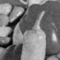
peppers	$\sigma_{n}=30$	$T=1.35$	$r=s=3$	$r=s=5$

Figure 3: Comparison of homogeneous diffusion (HD) and denoising by inpainting with regular masks (DbI-R) on the test image peppers with $\sigma_{n}=30$. Figure 3(c) and Figure 3(d) show the visual similarities of both methods. The diffusion time $T$ for homogeneous diffusion has been chosen to maximize the similarity to the denoising by inpainting result. Figure 3(d) and Figure 3(e) illustrate the influence of the expected density $\frac{1}{N}\|\mathbb{E}[\bm{c}]\|_{1}$ on the smoothness of the reconstruction: Figure 3(e) was intentionally chosen with a density that is too low resulting in too much smoothing.

The similarity between the methods can not only be observed visually, but also established theoretically. Next we provide a derivation in the 1-D case for regular grid masks relating the diffusion time of homogeneous diffusion to the mask density in DbI. Using the relationship from the 1-D case as an ansatz we experimentally find a relationship for the 2-D case.

4.1.1 Theoretical Analysis in 1D

We consider a discrete 1-D signal $\bm{f}$ and regular inpainting masks with spacing $r$ and shift $p\in\{0,\dots,r-1\}$. It is known that in 1D, homogeneous diffusion inpainting and linear interpolation are equivalent. Thus, an inpainted pixel at position $i$ can be described in terms of its two neighboring mask pixels. We denote the distance between the pixel $i$ and its neighboring mask pixel on the left by $\ell\coloneqq|i-p|\bmod r$, which implies that for mask pixels we have $\ell=0$. Accordingly, the distance to the mask pixel on the right is given by $r-\ell$. The interpolated value at pixel $i$ for mask $\ell+1$ is then

(25) $$v_{i}^{\ell+1}=\frac{r-\ell}{r}f_{i-\ell}+\frac{\ell}{r}f_{i+r-\ell}.$$

To obtain the final result, the inpaintings from the $r$ shifted masks are averaged. We get

(26) $$\begin{split}u_{i}=\frac{1}{r}\sum_{\ell=0}^{r-1}v_{i}^{\ell+1}&=\frac{1}{r}\left(f_{i}+\sum_{\ell=1}^{r-1}\frac{r-\ell}{r}f_{i-\ell}+\frac{\ell}{r}f_{i+r-\ell}\right)\\ &=\frac{1}{r^{2}}\left(rf_{i}+\sum_{\ell=1}^{r-1}\ell\left(f_{i-(r-\ell)}+f_{i+(r-\ell)}\right)\right),\end{split}$$

where the last line reveals the general form of the filter in dependence of the spacing $r$: The filter is given by a hat kernel with central weight $1/r$ and width $2r-1$. In Theorem 4.1 we demonstrate that this kernel can be seen as a consistent discretization of $\partial_{t}u=\partial_{xx}u$. Consequently, convolution with such a kernel approximates Gaussian smoothing, which explains the visual similarity of the results in Figure 3. Since the spacing $r$ determines the size of the smoothing kernel, we explicitly see the connection between the mask density and the smoothing strength. For the special case of $r=2$, Eq. 26 yields

(27) $$u_{i}=\frac{f_{i-1}+2f_{i}+f_{i+1}}{4},$$

which is exactly a single step of an explicit scheme for homogeneous diffusion with step size $T=\frac{1}{4}$ and initial signal $\bm{f}$ (assuming grid size $h=1$). If we reformulate Eq. 26 in a way that resembles an explicit scheme for homogeneous diffusion, we can derive a general connection between the spacing $r$ (and thus the density) of denoising by inpainting with regular masks and the time step size of such an explicit scheme, which we state in Theorem 4.1.

Theorem 4.1 (Connection between mask density and diffusion time).

Given the $r$ shifted regular inpainting masks in 1D, each of density $d=1/r$, denoising by inpainting approximates explicit homogeneous diffusion at time

$$T=\frac{1-d^{2}}{12d^{2}}.$$

Proof 4.2.

In Eq. 26 we derived the general form of the filter corresponding to denoising by inpainting with regular masks of spacing $r$ as

(28) $$u_{i}=\frac{1}{r^{2}}\left(rf_{i}+\sum_{\ell=1}^{r-1}\ell\left(f_{i-(r-\ell)}+f_{i+(r-\ell)}\right)\right).$$

We can rewrite this in the following manner:

(29) $$\begin{split}u_{i}&=\frac{1}{r^{2}}\left(rf_{i}+\sum_{\ell=1}^{r-1}\ell\left(f_{i-(r-\ell)}+f_{i+(r-\ell)}\right)\right)\\ &=\frac{1}{r^{2}}\left(r^{2}f_{i}-2\sum_{\ell=1}^{r-1}\ell f_{i}+\sum_{\ell=1}^{r-1}\ell\left(f_{i-(r-\ell)}+f_{i+(r-\ell)}\right)\right)\\ &=f_{i}+\frac{1}{r^{2}}\sum_{\ell=1}^{r-1}\ell\left(f_{i-(r-\ell)}-2f_{i}+f_{i+(r-\ell)}\right),\end{split}$$

where we have used that $\sum_{\ell=1}^{r-1}\ell=\frac{(r-1)r}{2}$. Then we may write

(30) $$\begin{split}u_{i}-f_{i}&=\frac{1}{r^{2}}\sum_{\ell=1}^{r-1}\ell\left(f_{i-(r-\ell)}-2f_{i}+f_{i+(r-\ell)}\right)\\ &=\frac{1}{r^{2}}\sum_{\ell=1}^{r-1}\ell(r-\ell)^{2}\,\frac{f_{i-(r-\ell)}-2f_{i}+f_{i+(r-\ell)}}{(r-\ell)^{2}}\\ &=\sum_{\ell=1}^{r-1}\frac{\ell(r-\ell)^{2}}{r^{2}}\,\frac{f_{i-(r-\ell)}-2f_{i}+f_{i+(r-\ell)}}{(r-\ell)^{2}}.\end{split}$$

By approximating $f_{i\pm(r-\ell)}$ via a Taylor expansion and using the sampling distance $h$, we can derive the time step size as

(31) $$\begin{split}u_{i}-f_{i}&=\sum_{\ell=1}^{r-1}\frac{\ell(r-\ell)^{2}}{r^{2}}\,\frac{f_{i-(r-\ell)}-2f_{i}+f_{i+(r-\ell)}}{(r-\ell)^{2}}\\ &=\sum_{\ell=1}^{r-1}\left(\frac{\ell(r-\ell)^{2}}{r^{2}}\right)\left(h^{2}\left.\partial_{xx}f\right|_{i}+\frac{h^{4}(r-\ell)^{2}}{12}\left.\partial_{xxxx}f\right|_{i}+\mathcal{O}(h^{6})\right)\\ &=h^{2}\sum_{\ell=1}^{r-1}\left(\frac{\ell(r-\ell)^{2}}{r^{2}}\right)\left(\left.\partial_{xx}f\right|_{i}+\mathcal{O}(h^{2})\right)\\ &\approx h^{2}\sum_{\ell=1}^{r-1}\left(\frac{\ell(r-\ell)^{2}}{r^{2}}\right)\left.\partial_{xx}f\right|_{i}\\ &\approx\left(h^{2}\sum_{\ell=1}^{r-1}\left(\frac{\ell(r-\ell)^{2}}{r^{2}}\right)\right)\frac{f_{i-1}-2f_{i}+f_{i+1}}{h^{2}}.\end{split}$$

We end up with an approximation of an explicit scheme with time step size

(32) $$T=h^{2}\sum_{\ell=1}^{r-1}\frac{\ell(r-\ell)^{2}}{r^{2}}=\frac{h^{2}(r^{2}-1)}{12}.$$

Using that the density is the inverse of the grid spacing and setting $h=1$, we derive the final relation between $T$ and the density $d$, given by

(33) $$T=\frac{1-d^{2}}{12d^{2}}.$$

To confirm that this relation allows for a good estimate of the diffusion time in practice, we perform an experiment on a one-dimensional signal, which is generated by extracting the 128th row of the peppers test image. Homogeneous diffusion is implemented using explicit Euler and the spatial discretization from Eq. 27 with the number of iterations chosen such that the desired diffusion time $T$ is reached. The experiment in Fig. 4 demonstrates that the diffusion time obtained via Theorem 4.1 is a good approximation.

(a) $r=5,T=2.0$	(b) $r=10,T=8.25$

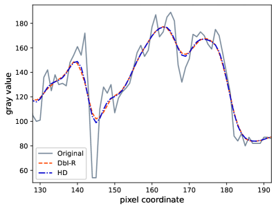
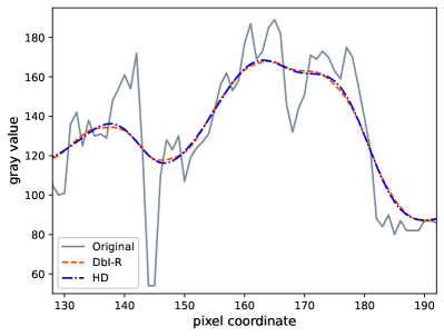
Figure 4: Comparison of denoising by inpainting with shifted regular masks (DbI-R) and homogeneous diffusion (HD) on a one-dimensional signal (128th row of the test image peppers). We display a section from the original signal and filtered versions obtained with denoising by inpainting with regular masks of spacing $r$ and homogeneous diffusion filtering with diffusion time $T$, calculated according to Theorem 4.1. We see that both filters lead to very similar results, confirming that the approximation from the theorem is indeed realistic.

4.1.2 Analysis in 2D

To derive the relationship to the diffusion time in the 1-D case we use the fact that the solution of the Laplace equation with Dirichlet boundaries is given by linear interpolation. That is, we know the closed form of the inpainting echoes in 1D. In 2D a closed form solution for those is not known, however they may be computed numerically. Thus our goal is to establish a relationship between the diffusion time and the density numerically.

We take as a starting point the ansatz from the 1-D case that the diffusion time $T$ is given as $\frac{1-d^{2}}{12d^{2}}$, but generalize it to the form $T\approx\frac{1-d^{\gamma}}{\beta d^{\gamma}}$. Provided that this conjecture is correct we only need to find the constants $\beta$ and $\gamma$. Since regular masks only allow for a stepwise adaptation of the mask density, they are not well-suited for generating a large number of data points at different densities. Therefore, we use uniform random masks instead. Note that they have, just like regular masks, a constant expectation, i.e., $\mathbb{E}[\bm{c}]=\text{const}$.

First we numerically tabulate the relationship between the density and the diffusion time. That is, given a density $d$ we find the diffusion time $T(d)$ which minimizes the difference between the filter matrices:

(34) $$T(d)=\underset{T\geq 0}{\operatorname*{\textrm{argmin}}}\,\|\bm{A}_{DbI}(d)-\bm{A}_{HD}(T)\|^{2}_{F}.$$

Here $\|\cdot\|_{F}$ is the Frobenius norm, and the matrices are the DbI filter matrix resulting from a probability mass function for masks with expected density $d$, and the matrix modeling homogeneous diffusion at time $T$ using an implicit Euler discretization:

(35) $$\bm{A}_{DbI}(d) \coloneqq\mathbb{E}\left[\left(\bm{C}+\left(\bm{I}-\bm{C}\right)\bm{L}\right)^{-1}\bm{C}\right],\quad\frac{1}{N}\|\mathbb{E}[\bm{c}]\|_{1}=d,$$

(36) $$\bm{A}_{HD}(T) \coloneqq\left(\bm{I}+T\bm{L}\right)^{-1}.$$

We estimate $\bm{A}_{DbI}$ using 1024 sampled masks. Then, having the relationship $d\mapsto T(d)$ we find that $T(d)\approx\frac{1-d^{\gamma}}{\beta d^{\gamma}}$ for $\beta=4.58$, $\gamma=1.3$, which is illustrated in Figure 5.

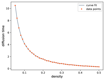
Figure 5: The fit based on the ansatz $\frac{1-d^{\gamma}}{\beta d^{\gamma}}$ with $\beta=4.58$, $\gamma=1.3$ and the tabulated correspondence between density and diffusion time. The results are obtained with denoising by inpainting with uniform random masks and an implicit scheme for homogeneous diffusion.

4.2 Adaptive Masks

A notable drawback of the regular grid masks is the space-invariant smoothing behavior. To retain important structures with homogeneous diffusion inpainting it is necessary to optimize the inpainting masks for the given image. There exist a number of mask selection strategies for the noise-free case, some of which we now consider and adapt to our setting.

4.2.1 Densification Method

Among the most successful mask selection strategies are probabilistic sparsification [61] and densification [43], which build the mask in an iterative way using a top-down and a bottom-up strategy, respectively.

In probabilistic sparsification, one starts with a full mask and takes away the least important pixels from a number of randomly selected candidates in each iteration. To identify those pixels, one temporarily excludes all candidates from the mask and computes an inpainting. Then the candidate locations with the highest local (i.e., pixelwise) reconstruction error are added back to the mask as they are assumed to be the most important, while the others remain permanently excluded. This process is repeated until the desired mask density is reached. In probabilistic densification, the initial mask is empty and again a number of candidate pixels are selected. Given an inpainting with the current mask (in the first step some pixels have to be chosen at random) one selects and adds those candidates to the mask that have the highest local reconstruction error.

In the noisy setting, special care is required as the pixel selection based on the local reconstruction error is not reliable. The local error does not allow the algorithm to distinguish between noise and important image structures, such as edges. If a pixel contains strong noise, this creates a large local error because – just like edges – the noise cannot be reconstructed by the smooth inpainting. Introducing such a noisy pixel into the mask is not desirable. We cure this problem by judging the importance of a pixel based on its effect on the global reconstruction error. We do this by calculating a full inpainting for each candidate pixel. While this improves the quality of the selected mask, it drastically increases the run time.

While in the noise-free setting densification and sparsification yield results of comparable quality [42], this is different when handling noisy data. For sparsification we initially have very dense masks. If we exclude candidate pixels from such masks, the reconstructions often only differ at the locations of these pixels. Therefore, sparsification tends to keep noisy pixels in the mask, even when a global reconstruction error is computed. This problem does not occur in probabilistic densification, as for a sparse mask, the candidate pixels have a global influence. The result of this effect is illustrated in Figure 6. Here, densification is able to select appropriate pixels that lead to an almost perfect result while sparsification fails to reconstruct the image properly.

Thus, we opt for a probabilistic densification algorithm based on a global error computation, which is described in Algorithm 1 and has been proposed in [1]. An additional advantage of this probabilistic densification method is that it does not only select pixels at useful locations (e.g., close to edges), but also implicitly avoids picking pixels that are too noisy, as they would have a negative impact on the reconstruction quality. The method can be interpreted according to the probabilistic mask generation framework from Section 3. The calculation of the corresponding probability mass function can be found in Appendix A.

(a) input	(b) sparsification	(c) densification
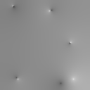
original	MSE: $76.07$	MSE: $1.98$
noisy ($\sigma_{n}=30$)	optimized mask	optimized mask

Figure 6: Comparison of sparsification and densification on a synthetic test image with $\sigma_{n}=30$ [1]. For both methods, the mask density $d$ was optimized with a grid search w.r.t. the MSE. The noisy gradient image is not reconstructed adequately by sparsification, since it favors keeping noisy pixels in the first iterations due to localization. Densification does not suffer from this problem and thereby achieves a better denoised reconstruction.

Algorithm 1 Mask densification with global error computation [1].

 

Input:

Noisy image $\bm{f}\in\mathbb{R}^{N}$, number of candidates $\alpha$, desired final mask density $d$.

Initialization:

Mask $\bm{c}=0$ is empty.

Compute:

do

1. Choose randomly a set $A\subset\{k\in\{1,...,N\}\,|\,c_{k}=0\}$ with $\alpha$ candidates.
   for all $i\in A$ do

   1. Set temporary mask $\bm{m}^{i}$ such that $\forall k\in\{1,...,\alpha\}\setminus\{i\}:m^{i}_{k}=c_{k}$, $m^{i}_{i}=1$.

   2. Compute reconstruction $\bm{u}^{i}$ from mask $\bm{m}^{i}$ and image data $\bm{f}$.

   end for

2. Set $\bm{c}=\underset{\bm{m}^{i},\,i\,\in A}{\operatorname*{\textrm{argmin}}}\,\textnormal{MSE}(\bm{u}^{i},\bm{f})$. This adds one mask point to $\bm{c}$.

while pixel density of $\bm{c}$ smaller than $d$.

Output:

Mask $\bm{c}$ of density $d$.
 

4.2.2 Analytic Method

As the global error computation in the previous approach requires calculating an inpainting for each candidate pixel, the run time is substantial. Therefore, we propose another approach, with the goal of a faster mask generation process. Belhachmi et al. [8] have shown that the mask density for homogeneous diffusion inpainting should be proportional to the pointwise magnitude of the Laplacian $|\bm{L}\bm{f}|$. Additionally, they suggest using the Gaussian-smoothed version $\bm{f}_{\sigma}\coloneqq\bm{K}_{\sigma}\ast\bm{f}$ of $\bm{f}$ even in the noise-free setting. Here $\bm{K}_{\sigma}$ is a discrete approximation of a Gaussian with standard deviation $\sigma$. This step proves even more beneficial in our setting, since we are calculating the Laplacian of noisy data, and regularizing $\bm{f}$ helps considerably for constructing a reasonable guidance image $|\bm{L}\bm{f}_{\sigma}|$.

As we require multiple different binary masks for our framework, we sample from $|\bm{L}\bm{f}_{\sigma}|$ by using a simple and fast Poisson sampling. Given a density image $\bm{d}\in[0,1]^{N}$, we can sample a mask according to it by generating a uniform random number $v_{i}\sim U[0,1]$ for each pixel $i$ and then thresholding at $d_{i}$:

(37) $$c_{i}=\begin{cases}1&\text{if }v_{i}\leq d_{i},\\ 0&\text{if }v_{i}>d_{i}.\end{cases}$$

Then the probability mass function $p_{\bm{d}}$ for sampling a mask $\bm{c}$ given the density image $\bm{d}$ is

(38) $$p_{\bm{d}}(\bm{c})=\frac{1}{P}\prod_{i=1}^{N}(d_{i})^{c_{i}}(1-d_{i})^{1-c_{i}},\quad P=\sum_{\bm{c}\in\{0,1\}^{N}}\prod_{i=1}^{N}(d_{i})^{c_{i}}(1-d_{i})^{1-c_{i}}.$$

By construction the mask would have an expected density equal to the mean value of $\bm{d}$. In our approach we set the per pixel probabilities to

(39) $$\bm{d}=\min\left\{C|\bm{L}\bm{f}_{\sigma}|,\bm{1}\right\},$$

where the minima are taken pointwise, and $C$ is a constant chosen such that the mean value of $\bm{d}$ is equal to the desired mask density. Figure 7 shows the pipeline for mask generation with this method. One can observe in Figure 7(b) that $\bm{d}$ is strongly affected by the noise despite the pre-smoothing. This is because we calculate second-order derivatives that are even more sensitive to noise. When sampling from this image the mask is drawn towards noisy pixels. To counteract this, we propose to perform an additional outer smoothing of the probability image $\bm{d}$, after the absolute value of the Laplacian is taken, thus modifying it to

(40) $$\bm{d}=\min\left\{C\left(\bm{K}_{\rho}\ast|\bm{L}\bm{f}_{\sigma}|\right),\bm{1}\right\},$$

with a post-smoothing parameter $\rho$. Our proposed selection strategy offers an instant generation of adaptive masks, in a sense that it does not require the calculation of any inpainting. On the other hand, contrary to probabilistic densification it does not have a mechanism to avoid noisy mask pixels. To obtain the best possible results, the pre-smoothing parameter $\sigma$, the post-smoothing parameter $\rho$, and the desired mask density have to be optimized depending on the image content and the noise level.

Note that Belhachmi et al. [8] apply Floyd-Steinberg dithering [35], which includes an error diffusion in the binarization process. This strategy can be equipped with a random component in order to generate multiple masks, which makes it an alternative to Poisson sampling for us. We have tested both methods and found that there is no advantage in using Floyd-Steinberg dithering, thus we opt for the simple Poisson sampling. Nonetheless, we give the mask probabilities for sampling with error diffusion methods in Appendix B.

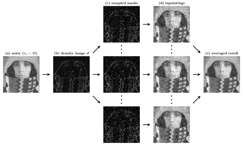
Figure 7: Pipeline for mask generation with the analytic method. (a) Test image trui with $\sigma_{n}=30$. (b) Target image (without post-smoothing) from which masks are sampled. (c) Three examples of Poisson-sampled masks. (d) Corresponding homogeneous diffusion inpaintings. (e) Averaged inpaintings (from 32 masks), final denoising result.

5 Experiments

To assess the denoising capacities of our proposed framework, we first evaluate the results for the different spatial optimization methods. As our main goal is insights about our denoising by inpainting models, we compare them to PDE-based methods of similar structural complexity. Therefore, we choose homogeneous diffusion, linear space-variant diffusion, nonlinear diffusion, and TV regularization for comparison. Furthermore, we investigate how tonal optimization affects the denoising quality of our models. Then we study denoising by biharmonic inpainting as a representative of a higher-order linear inpainting operator. Lastly, we test the convergence with low-discrepancy sequences from Section 3.1.3.

5.1 Experimental Setup

We evaluate the framework on three standard test images (trui, peppers, walter) with a resolution of $256\times 256$, that are corrupted with additive Gaussian noise with standard deviations $\sigma_{n}\in\{10,20,30\}$ that we do not clip. To ensure a fair comparison, we optimize the mask density and if required the pre- and post-smoothing parameter for the denoising by inpainting methods w.r.t. the MSE to the original image. We do this individually for each image and for each noise level using a grid search. In practice, these parameters need to be adapted to the noise level and the image content. We create 32 masks with each of the mask selection methods, except for the regular masks where the number is determined by the spacing and thus by the density. For the proposed probabilistic densification algorithm we set the number of candidate pixels per iteration to 16.

5.2 Spatial Mask Selection

In a first step, we investigate the different spatial selection strategies proposed in Section 4 and compare the denoising results with the standard diffusion methods presented in Section 2.1 as well as with TV regularization [74]. For the diffusion methods we optimize the stopping time and if required the contrast parameter of the Charbonnier diffusivity [21]. For TV regularization we optimize the regularization parameter.

As can be seen in Table 1, inpainting with regular masks leads to unsatisfying results, slightly worse than those obtained with homogeneous diffusion filtering. This is expected given the connections derived in Section 4.1. Note that the stopping time in homogeneous diffusion filtering can be tuned continuously, while the spacing of the regular mask can only be adapted in integer steps. The analytic method based on Poisson sampling of the smoothed Laplacian magnitude improves the results, especially at lower noise levels. Figure 8(c) shows how the mask pixels accumulate around important image structures, enabling an edge-preserving filtering behavior. The densification method is able to further improve those results. The reason for this improvement can be seen in Figure 8(d). On top of selecting pixels at reasonable positions, the error in the mask is reduced drastically in comparison to the analytic method, because the methods implicitly avoids noisy pixels. The adaptive mask selection strategies enable the denoising by inpainting method to produce results that are similar or even superior to linear space-variant diffusion filtering. Nevertheless, it cannot reach the quality of nonlinear diffusion. This is not surprising, as a feedback mechanism throughout the inpainting process is missing. The quality of TV regularization on the other hand is matched by the densification method on the test image trui.

Although qualitatively the densification approach is better than the analytic method, its required run time is orders of magnitude larger, and this only gets worse for images of higher resolution. Due to the required number of inpaintings, the densification method takes about an hour to create a single mask with 10% density for our $256\times 256$ pixel test images. In contrast, the analytic and the regular approaches allow instant mask creation in approximately a millisecond. Thus, our analytic method yields a reasonable spatial mask pixel distribution in a very short time and clearly has potential, if the error in the mask pixels can be reduced. To this end, we complement the mask selection strategies with tonal optimization.

Table 1: Results (MSE) for denoising by inpainting with regular masks, the densification method and the analytic method with 32 masks (less masks for the regular mask method). Comparison to classical diffusion-based denoising methods and TV regularization.

	trui			peppers			walter
noise level $\sigma_{n}$	$10$	$20$	$30$	$10$	$20$	$30$	$10$	$20$	$30$
regular	$27.30$	$57.29$	$86.46$	$35.31$	$64.40$	$91.79$	$22.63$	$50.13$	$79.16$
densification	$19.34$	$42.72$	$68.01$	$24.36$	$47.27$	$69.89$	$13.40$	$29.65$	$47.65$
analytic	$21.49$	$49.71$	$79.79$	$25.14$	$51.70$	$79.91$	$16.41$	$37.83$	$62.08$
homogeneous	$24.12$	$50.18$	$76.12$	$32.16$	$59.77$	$84.58$	$19.65$	$42.76$	$66.87$
linear space-variant	$20.10$	$47.07$	$74.13$	$24.99$	$51.77$	$78.27$	$15.06$	$37.22$	$62.10$
nonlinear	$\bm{16.55}$	$\bm{36.32}$	$\bm{56.63}$	$\bm{22.17}$	$\bm{40.90}$	$\bm{58.75}$	$\bm{11.97}$	$\bm{26.33}$	$\bm{41.76}$
TV regularization	$19.70$	$43.53$	$68.07$	$23.45$	$44.57$	$65.22$	$14.91$	$32.57$	$50.89$

(a) input	(b) regular	(c) densification	(d) analytic
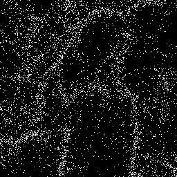
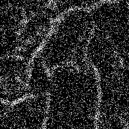
original	Mask MSE: $405.09$	Mask MSE: $345.23$	Mask MSE: $410.63$
noisy ($\sigma_{n}=20$)	MSE: $64.40$	MSE: $47.27$	MSE: $51.70$

Figure 8: Results for denoising by inpainting with 32 masks (six masks for the regular mask method) for the different spatial optimization methods on the test image peppers with $\sigma_{n}=20$. Top row: (a) original image, (b)-(d) one representative out of all the masks for every method. The MSE is computed at mask pixels. Bottom row: (a) noisy image, (b)-(d) denoising by inpainting results with optimized parameters and the MSE in the entire image. We see that our analytic method and the densification method adapt the mask point locations to the structure of the image. Densification additionally avoids choosing noisy mask pixels, leading to a smaller error in the mask pixels and eventually to a better reconstruction.

5.3 Tonal Optimization

To evaluate the effect of tonal optimization, we apply it to the masks obtained by each of our spatial optimization methods. We optimize the tonal values for each individual mask, before once again averaging the respective inpaintings to obtain the final denoised result.

The results in Table 2 reveal that the methods that do not consider the noise in the selection process get the greatest boost in performance. This confirms the conjecture that tonal optimization is able to mitigate the negative effect of noisy mask pixels selection. We also observe that tonal optimization decreases the error for the mask pixels for those methods. In Figure 8, the MSE at mask locations decreases from 405.09 to 271.80 for the regular mask, and from 410.63 to 306.62 for the analytic method. For probabilistic densification, tonal optimization barely changes the final results (see Table 1 and Table 2), as well as the mask MSE (which even increases slightly from 345.23 to 356.12 in the example).

Thus, tonal optimization enables our proposed analytic method to produce results comparable in quality to those of the densification method. Although the tonal optimization step takes some additional seconds, the analytic method with tonal optimization is still orders of magnitude faster than the densification method. Figure 9 shows a selection of resulting images comparing the two adaptive methods with tonal optimization.

Table 2: Results (MSE) for denoising by inpainting with regular masks, the densification method and the analytic method with 32 masks (less masks for the regular mask method) including tonal optimization.

	trui			peppers			walter
noise level $\sigma_{n}$	$10$	$20$	$30$	$10$	$20$	$30$	$10$	$20$	$30$
regular	$22.32$	$48.77$	$76.06$	$32.65$	$60.92$	$87.05$	$16.36$	$39.54$	$64.45$
densification	$18.46$	$41.56$	$67.72$	$24.42$	$47.28$	$70.21$	$12.35$	$28.13$	$45.92$
analytic	$\bm{17.24}$	$\bm{39.49}$	$\bm{63.17}$	$\bm{23.68}$	$\bm{46.43}$	$\bm{68.55}$	$\bm{12.08}$	$\bm{27.66}$	$\bm{45.36}$

(a) original	(b) noisy	(c) densification	(d) analytic
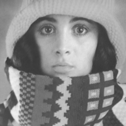
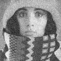
trui	$\sigma_{n}=30$	MSE: $67.72$	MSE: $63.17$
peppers	$\sigma_{n}=20$	MSE: $47.28$	MSE: $46.43$
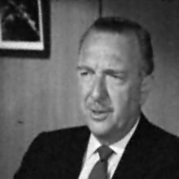
walter	$\sigma_{n}=10$	MSE: $12.35$	MSE: $12.08$

Figure 9: Visual comparison of denoising by inpainting with the densification method and the analytic method on three test images with noise. Both methods are using tonal optimization.

5.4 Biharmonic Inpainting

Another interesting test case consists of evaluating higher order polyharmonic operators. It has been shown that the biharmonic operator can have quality advantages over homogeneous diffusion (i.e., the harmonic operator) in classical sparse inpainting [22, 37, 75]. Biharmonic inpainting is given by the PDE

(41) $$\bigl{(}c(\bm{x})+(1-c(\bm{x}))\Delta^{2}\bigr{)}u(\bm{x})=c(\bm{x})f(\bm{x})\quad\text{for }\bm{x}\in\Omega,$$

with $\Delta^{2}u=\partial_{xxxx}u+2\partial_{xxyy}u+\partial_{yyyy}u$ and reflecting boundary conditions $\partial_{\bm{n}}u(\bm{x})=0$ and $\partial_{\bm{n}}\Delta u(\bm{x})=0$ for $\bm{x}\in\partial\Omega$. It can be derived from the following variational formulation (analogously to Eq. 12):

(42) $$\min_{u}\int_{\Omega}(\Delta u(\bm{x}))^{2}\,d\bm{x},\textrm{ such that }u(\bm{x})=f(\bm{x})\textrm{ for }\bm{x}\in K.$$

This shows that biharmonic inpainting penalizes second-order derivatives. Biharmonic inpainting does not suffer from the typical singularities at mask points that homogeneous diffusion inpainting produces. On the other hand it can produce over- and undershoots, since it does not guarantee a maximum-minimum principle. We evaluate the potential of biharmonic inpainting for denoising by comparing it to homogeneous diffusion inpainting. To ensure that the results reflect the quality of the operators, we perform the experiment on fully random masks.

Our results in Table 3 show that biharmonic inpainting does lead to an improvement, and it is largest at low noise levels. This is to be expected, as the method promotes less smoothness than homogeneous diffusion inpainting, by penalizing second degree derivatives instead of first degree. However, if tonal optimization is applied, this advantage is neutralized and the two methods perform similarly. Figure 10 displays the results for peppers at noise level $\sigma_{n}=30$. These results support our reasoning that data optimization plays a significant role for the denoising abilities of our framework, being more important than the use of more complex, higher-order models. Further experiments on spatially optimized masks (see Table 4) confirm our findings, and even shift the advantage towards homogeneous diffusion inpainting. When comparing these experiments to results from classical sparse image inpainting, one has to consider that the singularities, that homogeneous diffusion inpainting suffers from, are suppressed by the averaging in the DbI framework. Thus, this disadvantage of homogeneous diffusion inpainting does not come into play in our scenario. Lastly, one should keep in mind that biharmonic inpainting leads to a higher condition number of the inpainting matrix, and consequently each inpainting is numerically more burdensome and less efficient.

Table 3: Results (MSE) for denoising by inpainting with 32 random masks using homogeneous diffusion (HD) and biharmonic (BI) inpainting, without and with tonal optimization (TO).

	trui			peppers			walter
noise level $\sigma_{n}$	$10$	$20$	$30$	$10$	$20$	$30$	$10$	$20$	$30$
HD, without TO	$30.53$	$65.51$	$100.51$	$36.01$	$71.20$	$104.21$	$26.93$	$60.21$	$94.37$
BI, without TO	$\bm{24.23}$	$\bm{56.37}$	$\bm{93.51}$	$\bm{33.28}$	$\bm{66.61}$	$\bm{102.49}$	$\bm{19.16}$	$\bm{48.19}$	$\bm{82.92}$
HD, with TO	$23.10$	$49.83$	$\bm{76.57}$	$\bm{31.98}$	$\bm{59.75}$	$\bm{85.28}$	$18.09$	$41.79$	$66.40$
BI, with TO	$\bm{22.21}$	$\bm{49.74}$	$77.25$	$33.27$	$61.84$	$87.92$	$\bm{16.52}$	$\bm{39.53}$	$\bm{65.03}$

(a) HD	(b) HD + TO	(c) BI	(d) BI + TO
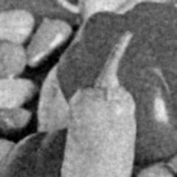
MSE: $104.21$	MSE: $85.28$	MSE: $102.49$	MSE: $87.92$

Figure 10: Results for denoising by homogeneous diffusion (HD) inpainting and biharmonic (BI) inpainting on the test image peppers with $\sigma_{n}=30$. Both methods are using 32 random masks. We display results without and with tonal optimization (TO).

Table 4: Results (MSE) for denoising by inpainting with 32 masks obtained with the analytic method using homogeneous diffusion (HD) and biharmonic (BI) inpainting, without and with tonal optimization (TO).

	trui			peppers			walter
noise level $\sigma_{n}$	$10$	$20$	$30$	$10$	$20$	$30$	$10$	$20$	$30$
HD, without TO	$21.49$	$49.71$	$\bm{79.79}$	$\bm{25.14}$	$\bm{51.70}$	$\bm{79.91}$	$16.41$	$37.83$	$\bm{62.08}$
BI, without TO	$\bm{19.01}$	$\bm{47.47}$	$82.39$	$25.83$	$55.42$	$90.28$	$\bm{14.16}$	$\bm{37.15}$	$68.25$
HD, with TO	$17.24$	$\bm{39.49}$	$\bm{63.17}$	$\bm{23.68}$	$\bm{46.43}$	$\bm{68.55}$	$12.08$	$27.66$	$\bm{45.36}$
BI, with TO	$\bm{17.18}$	$40.45$	$66.13$	$25.35$	$49.27$	$72.68$	$\bm{11.74}$	$\bm{27.22}$	$45.70$

5.5 Low-Discrepancy Sampling

As mentioned in Section 3.1.3, the goal of using low-discrepancy sequences is faster convergence. We test if we can exploit this in our analytic method by replacing Poisson sampling by sampling with a low-discrepancy sequence. In our experiments we use the R2 low-discrepancy sequence [72] to create a sampling threshold in each pixel (see [72] for details). This leads to a more regular sampling pattern compared to Poisson sampling.

Our results in Table 5 show that when no tonal optimization is applied, the low-discrepancy sequences lead to better results than Poisson sampling for 32 masks. The plots in Figure 11 show that this also holds consistently over all mask counts. Equivalently, they show that one can achieve the same results as Poisson sampling for a substantially lower mask number. Interestingly, in Table 5 there are some cases where this sampling strategy yields results even superior to Poisson sampling with tonal optimization performed additionally. This, however, changes for larger mask numbers (see Figure 11), where tonal optimization with Poisson sampling yields better results consistently. Unfortunately, the low-discrepancy sampling does not benefit as much from tonal optimization as Poisson sampling. Even though it yields the slightly better results on trui and walter than its Poisson-sampled counterpart, it performs worse on peppers. For large numbers of masks, the results become very similar, although on average, Poisson sampling is slightly better. In general, our results show that low-discrepancy sequences can be an attractive choice if one does not want to apply tonal optimization. If tonal optimization is used, the two strategies yield similar results. For a small number of masks, low-discrepancy sequences have a small advantage. However, if one has no restriction on the number of masks, Poisson sampling should be preferred.

Table 5: Results (MSE) for denoising by inpainting with 32 masks for the analytic method with Poisson sampling (PS) vs. low-discrepancy sampling (LD), without and with tonal optimization (TO).

	trui			peppers			walter
noise level $\sigma_{n}$	$10$	$20$	$30$	$10$	$20$	$30$	$10$	$20$	$30$
PS, without TO	$21.49$	$49.71$	$79.79$	$25.14$	$51.70$	$79.91$	$16.41$	$37.83$	$62.08$
LD, without TO	$18.68$	$42.35$	$68.10$	$\bm{23.47}$	$46.58$	$70.65$	$13.95$	$31.70$	$51.72$
PS, with TO	$17.24$	$39.49$	$63.17$	$23.68$	$\bm{46.43}$	$\bm{68.55}$	$12.08$	$27.66$	$45.36$
LD, with TO	$\bm{16.56}$	$\bm{38.53}$	$\bm{62.58}$	$24.13$	$46.98$	$69.01$	$\bm{11.30}$	$\bm{26.34}$	$\bm{43.83}$

(a) peppers with $\sigma_{n}=10$	(b) walter with $\sigma_{n}=30$

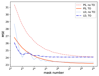
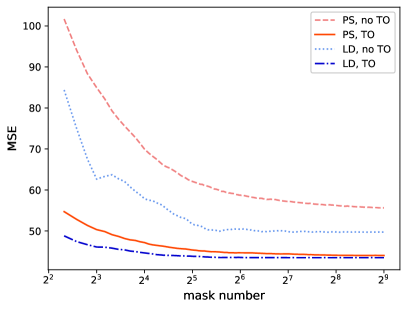
Figure 11: Results for denoising by inpainting with the analytic method with Poisson sampling (PS) vs. low-discrepancy sequence based sampling (LD), without and with tonal optimization (TO). We display the MSE in dependence of the mask number on two example test cases.

6 Conclusions

Our work is the first journal paper that analyzes the denoising abilities of PDE-based inpainting methods in a systematic way. Our denoising by inpainting (DbI) framework achieves denoising by averaging inpainting results with different sparse masks of the same density. We justify this approach both from a deterministic and a probabilistic viewpoint, and we provide convergence estimates for both.

In the 1-D case with homogeneous diffusion inpainting and shifted regular masks, we have established a one-to-one relationship between the mask density and the diffusion time. Space-variant filtering behavior can be achieved when we supplement homogeneous diffusion inpainting with adaptive data selection strategies.

Furthermore, we have presented two distinct, fundamental strategies for the adaptive data optimization. The densification method from our conference paper [1] aims at finding pixels that represent the data well. Thereby, it implicitly avoids the selection of noisy mask pixels during spatial optimization. On the contrary, we have proposed a new approach, where the selection of noisy pixels is tolerated in the spatial optimization but is compensated for by the tonal optimization. It leads to a considerable speedup while achieving superior quality.

While biharmonic inpainting can be more powerful than homogeneous diffusion inpainting [22, 37, 75], this can no longer be observed for denoising by inpainting with optimized data. This underlines the importance of choosing appropriate data over more complex operators.

Our work constitutes an unconventional, new approach to image denoising: By using a simple inpainting operator but focusing on adequate data selection we shift the priority from optimizing the filter model to optimizing the considered data. Moreover, our densification strategy allows us to find the most trustworthy pixels in the data. This shows that simple filter operators such as homogeneous diffusion can give deep insights into data. Last but not least, we have seen that the filling-in effect is not only useful in variational optic flow models and in PDE-based inpainting, but also in denoising. This emphasizes its fundamental role in digital image analysis, which is in full agreement with classical results from biological vision [85].

While our focus in the present paper is on gaining fundamental insights into the potential of inpainting ideas for denoising, our future work will deal with various modifications to make these ideas more competitive to state-of-the-art denoising methods. To this end, we are going to consider more sophisticated inpainting operators [75] and data selection strategies [29], including neural ones [4, 69], and the incorporation of more advanced types of data [47].

Appendix A Probability for Probabilistic Densification Masks

In the denoising framework of Adam et al. [1] a probabilistic densification algorithm is used in order to construct the masks. At the beginning of step $s+1$ the algorithm has already inserted $s$ mask pixels yielding the mask $\bm{c}^{s}$. At the end of step $s+1$ we want to have inserted a new mask pixel that is not in $\bm{c}^{s}$. Consequently, we can select a pixel only from the set $\mathcal{I}^{s}$, with $|\mathcal{I}^{s}|=N-s$ remaining empty mask pixel locations. The algorithm samples a set $\mathcal{X}$ of $\alpha$ distinct candidates from $\mathcal{I}^{s}$ uniformly at random (there are $C^{N-s}_{\alpha}$ different ways to do so):

(43) $$\mathcal{X}=\{X_{1},\ldots,X_{\alpha}\in\mathcal{I}^{s}\,:\,X_{i}\neq X_{j}\text{ for }i\neq j\}.$$

Then one chooses the candidate $X^{*}\in\mathcal{X}$ with lowest reconstruction error (w.r.t. the noisy image $\bm{f}$):

$$X^{*}\in\mathcal{X}^{*}=\underset{X\in\mathcal{X}}{\operatorname*{\textrm{argmin}}}\,E^{s}(X),\quad E^{s}(X)\coloneqq|\bm{r}(\bm{c}^{s}+\bm{e}_{X},\bm{f})-\bm{f}|^{2},$$

where $\bm{e}_{X}\in\mathbb{R}^{N}$ is the zero vector modified with a one at the location corresponding to mask point $X$. The minimizer does not have to be unique; in fact the set of minimizers

(44) $$\mathcal{X}^{*}=\{X_{i}\in\mathcal{X}\,:\,E^{s}(X_{i})=\min_{X\in\mathcal{X}}E^{S}(X)\}$$

may have more than one element ($|\mathcal{X}^{*}|>1$) in which case we choose $X^{*}$ uniformly at random from $\mathcal{X}^{*}$ with probability $\frac{1}{|\mathcal{X}^{*}|}$. This completes step $s+1$, now with a specific $X^{*}=x^{*}$ and corresponding mask $\bm{c}^{s+1}=\bm{c}^{s}+\bm{e}_{x^{*}}$. If the desired number of mask points have been achieved the algorithm ends, otherwise one proceeds to step $s+2$ in the exact same manner.

After we have inserted mask pixel $x^{*}\in\mathcal{I}^{s}$ we want to be able to compute the probability $\Pr(X^{*}=x^{*})$ of this occurring. This is equal to the probability of $x^{*}$ having been selected as a candidate:

(45) $$\Pr(x^{*}\in\mathcal{X})=C^{N-s-1}_{\alpha-1}/C^{N-s}_{\alpha}=\frac{\alpha}{N-s},$$

multiplied by the probability $\Pr(x^{*}\in\mathcal{X}^{*}\,|\,x^{*}\in\mathcal{X})$ that $x^{*}$ ends up in $\mathcal{X}^{*}$, which is in turn multiplied by the probability $\Pr(X^{*}=x^{*}\,|\,x^{*}\in\mathcal{X}^{*})=\frac{1}{|\mathcal{X}^{*}|}$ of having picked $x^{*}$ from $\mathcal{X}^{*}$ uniformly at random. We thus have the following chain of conditional probabilities:

(46) $$\begin{split}\Pr(X^{*}=x^{*})&=\Pr(X^{*}=x^{*}\,|\,x^{*}\in\mathcal{X}^{*})\Pr(x^{*}\in\mathcal{X}^{*})\\ &=\Pr(X^{*}=x^{*}\,|\,x^{*}\in\mathcal{X}^{*})\Pr(x^{*}\in\mathcal{X}^{*}\,|\,x^{*}\in\mathcal{X})\Pr(x^{*}\in\mathcal{X})\\ &=\frac{1}{|\mathcal{X}^{*}|}\Pr(x^{*}\in\mathcal{X}^{*}\,|\,x^{*}\in\mathcal{X})\frac{\alpha}{N-s}.\end{split}$$

We can rewrite the terms involving $\mathcal{X}^{*}$ in the following manner:

(47) $$\frac{1}{|\mathcal{X}^{*}|}\Pr(x^{*}\in\mathcal{X}^{*}\,|\,x^{*}\in\mathcal{X})=\sum_{\beta=1}^{\alpha}\frac{1}{\beta}\Pr(x^{*}\in\mathcal{X}^{*}\land|\mathcal{X}^{*}|=\beta\,|\,x^{*}\in\mathcal{X}).$$

The probability on the right-hand side can be rewritten as requiring $\beta$ of the candidates to have energy equal to $E^{s}(x^{*})$ and the remaining $\alpha-\beta$ having a strictly larger energy:

(48) $$\begin{gathered}\Pr(x^{*}\in\mathcal{X}^{*}\land|\mathcal{X}^{*}|=\beta\,|\,x^{*}\in\mathcal{X})=\\ =\Pr\left(\left(\bigwedge_{i=1}^{\beta}E^{s}(X_{i})=E^{s}(x^{*})\right)\land\left(\bigwedge_{j=\beta+1}^{\alpha}E^{s}(X_{j})>E^{s}(x^{*})\right)\,\Bigg{|}\,x^{*}\in\mathcal{X}\right).\end{gathered}$$

To compute the above probabilities we would need to know the total number of pixels from $\mathcal{I}^{s}$ with energy equal to $E^{s}(x^{*})$:

(49) $$N_{eq}\coloneqq|\{x\in\mathcal{I}^{s}\,:\,E^{s}(x)=E^{s}(x^{*})\}|,$$

and the total number of pixels from $\mathcal{I}^{s}$ having a strictly higher energy:

(50) $$N_{gt}\coloneqq|\{x\in\mathcal{I}^{s}\,:\,E^{s}(x)>E^{s}(x^{*})\}|.$$

From the requirement $|\mathcal{X}^{*}|=\beta$, it follows that we need to choose $\beta$ pixels that have energy equal to $E^{s}(x^{*})$. However, $x^{*}\in\mathcal{X}$ so $E^{s}(X)=E^{s}(x^{*})$ with probability $1$ for at least one candidate $X=x^{*}$. Then $\beta-1$ elements $X_{i}$ remain to be selected from $(N_{eq}-1)$ locations, the total number of possibilities being $C^{N_{eq}-1}_{\beta-1}$. Finally the remaining $\alpha-\beta$ candidates must be selected from $N_{gt}$ locations, resulting in $C^{N_{gt}}_{\alpha-\beta}$ options. Using this we can compute the probability

(51) $$\frac{1}{|\mathcal{X}^{*}|}\Pr(x^{*}\in\mathcal{X}^{*}\,|\,x^{*}\in\mathcal{X})=\sum_{\beta=1}^{\alpha}\frac{1}{\beta}\frac{C^{N_{eq}-1}_{\beta-1}C^{N_{gt}}_{\alpha-\beta}}{C^{N-s-1}_{\alpha-1}}.$$

Ultimately we get the following probability for a single step:

(52) $$\Pr(X^{*}=x^{*})=\frac{\alpha}{N-s}\sum_{\beta=1}^{\alpha}\frac{1}{\beta}\frac{C^{N_{eq}-1}_{\beta-1}C^{N_{gt}}_{\alpha-\beta}}{C^{N-s-1}_{\alpha-1}}=\sum_{\beta=1}^{\alpha}\frac{1}{\beta}\frac{C^{N_{eq}-1}_{\beta-1}C^{N_{gt}}_{\alpha-\beta}}{C^{N-s}_{\alpha}}.$$

Through the probabilistic densification procedure the exact same mask $\bm{c}$, with $|\bm{c}|$ mask pixels, can be constructed in $|\bm{c}|!$ different ways (the same set of mask pixels being introduced in all possible orders). That is, we get the probability mass function $p$ over masks that also retain the order of insertion of their mask pixels (e.g., we can modify $\bm{c}$ by setting entries equal to one, to be equal to $s$: the step in which those were inserted). To get the usual probability mass function over binary masks we need to sum up the above probabilities over all $|\bm{c}|!$ permutations of point insertion orders. The main issue for practicality is that $N_{eq}$ and $N_{gt}$ must be known, which would require evaluating all possible $|\mathcal{I}^{s}|=N-s$ inpaintings for a single step.

Appendix B Probability for Error Diffusion Masks

Error diffusion halftoning (e.g., Floyd-Steinberg dithering [35]) can be used to produce a binary mask $\bm{c}\in\{0,1\}^{N}$ from a continuous density image $\bm{d}\in[0,1]^{N}$. The process involves iterating over the image pixels (e.g., in serpentine order), binarizing a single pixel at a given step, and then diffusing the error arising from the binarization to the set of currently non-visited pixels. This results in a sequence of images $\bm{d}=\bm{d}^{1},\bm{d}^{2},\ldots,\bm{d}^{N+1}=\bm{c}$. The binarization happens according to a thresholding step, which usually reads $d^{k}_{k}<0.5\implies d^{k+1}_{k}=0,\,c_{k}=0$ and $d^{k}_{k}\geq 0.5\implies d^{k+1}_{k}=1,\,c_{k}=1$. Since we want to get multiple masks stochastically, we randomize the process by sampling a uniform random number $v_{k}\in[0,1]$ for pixel $k$, and then perform thresholding: $d^{k-1}_{k}\geq v_{k}\implies c_{k}=1$ and $d^{k-1}_{k}<v_{k}\implies c_{k}=0$. Then the probability mass function for mask $\bm{c}$ constructed from density image $\bm{d}$ is

(53) $$p_{\bm{d}}(\bm{c})=\frac{1}{P}\prod_{k=1}^{N}(d^{k}_{k}(\bm{c}))^{c_{k}}(1-d^{k}_{k}(\bm{c}))^{1-c_{k}},\quad P=\sum_{\bm{c}\in\{0,1\}^{N}}\prod_{k=1}^{N}(d^{k}_{k}(\bm{c}))^{c_{k}}(1-d^{k}_{k}(\bm{c}))^{1-c_{k}}.$$

In the above $d^{k}_{k}(\bm{c})$ are assumed to be clamped to $[0,1]$. Note that while this bears similarity to Poisson sampling, the probability $d^{k}_{k}(\bm{c})$ is conditional on the probabilities in the $k$ previous steps. However, algorithmically it is trivial to compute the numerator of the probability during the error diffusion process.

References

- [1] R. D. Adam, P. Peter, and J. Weickert, Denoising by inpainting, in Scale Space and Variational Methods in Computer Vision, F. Lauze, Y. Dong, and A. B. Dahl, eds., vol. 10302 of Lecture Notes in Computer Science, Springer, Cham, 2017, pp. 121–132.
- [2] C. Aguerrebere, A. Almansa, J. Delon, Y. Gousseau, and P. Musé, A Bayesian hyperprior approach for joint image denoising and interpolation, with an application to HDR imaging, IEEE Transactions on Computational Imaging, 3 (2017), pp. 633–646.
- [3] N. Ahmed, T. Natarajan, and K. Rao, Discrete cosine transform, IEEE Transactions on Computers, C-23 (1974), pp. 90–93.
- [4] T. Alt, P. Peter, and J. Weickert, Learning sparse masks for diffusion-based image inpainting, in Pattern Recognition and Image Analysis, A. J. Pinho, P. Georgieva, L. F. Teixeira, and J. A. Sánchez, eds., vol. 13256 of Lecture Notes in Computer Science, Springer, Cham, 2022, pp. 528–539.
- [5] S. Andris, P. Peter, R. M. K. Mohideen, J. Weickert, and S. Hoffmann, Inpainting-based video compression in FullHD, in Scale Space and Variational Methods in Computer Vision, A. Elmoataz, J. Fadili, Y. Quéau, J. Rabin, and L. Simon, eds., vol. 12679 of Lecture Notes in Computer Science, Springer, Cham, 2021, pp. 425–436.
- [6] J.-F. Aujol, S. Ladjal, and S. Masnou, Exemplar-based inpainting from a variational point of view, SIAM Journal on Mathematical Analysis, 42 (2010), pp. 1246–1285.
- [7] C. Barnes, E. Shechtman, A. Finkelstein, and D. B. Goldman, PatchMatch: A randomized correspondence algorithm for structural image editing, ACM Transactions on Graphics, 28 (2009), pp. 1–11.
- [8] Z. Belhachmi, D. Bucur, B. Burgeth, and J. Weickert, How to choose interpolation data in images, SIAM Journal on Applied Mathematics, 70 (2009), pp. 333–352.
- [9] J. M. Berger and G. J. Lasher, The use of discrete Green’s functions in the numerical solution of Poisson’s equation, Illinois Journal of Mathematics, 2 (1958), pp. 593–607.
- [10] M. Bertalmío, G. Sapiro, V. Caselles, and C. Ballester, Image inpainting, in Proc. SIGGRAPH 2000, New Orleans, LI, July 2000, pp. 417–424.
- [11] M. Bertalmío, L. Vese, G. Sapiro, and S. Osher, Simultaneous structure and texture image inpainting, IEEE Transactions on Image Processing, 12 (2003), pp. 882–889.
- [12] S. Bonettini, I. Loris, F. Porta, M. Prato, and S. Rebegoldi, On the convergence of a linesearch based proximal-gradient method for nonconvex optimization, Inverse Problems, 33 (2017), Article 055005.
- [13] M. Breuß, L. Hoeltgen, and G. Radow, Towards PDE-based video compression with optimal masks prolongated by optic flow, Journal of Mathematical Imaging and Vision, 63 (2021), pp. 144–156.
- [14] A. Bruhn and J. Weickert, A confidence measure for variational optic flow methods, in Geometric Properties from Incomplete Data, R. Klette, R. Kozera, L. Noakes, and J. Weickert, eds., vol. 31 of Computational Imaging and Vision, Springer, Dordrecht, 2006, pp. 283–297.
- [15] A. Buades, B. Coll, and J.-M. Morel, A review of image denoising algorithms, with a new one, Multiscale Modeling and Simulation, 4 (2005), pp. 490–530.
- [16] M. Burger, L. He, and C.-B. Schönlieb, Cahn–Hilliard inpainting and a generalization for grayvalue images, SIAM Journal on Imaging Sciences, 2 (2009), pp. 1129–1167.
- [17] S. Carlsson, Sketch based coding of grey level images, Signal Processing, 15 (1988), pp. 57–83.
- [18] R. H. Chan, C.-W. Ho, and M. Nikolova, Salt-and-pepper noise removal by median-type noise detectors and detail-preserving regularization, IEEE Transactions on Image Processing, 14 (2005), pp. 1479–1485.
- [19] T. F. Chan and J. Shen, Mathematical models for local nontexture inpaintings, SIAM Journal on Applied Mathematics, 62 (2001), pp. 1019–1043.
- [20] T. F. Chan and J. Shen, Non-texture inpainting by curvature-driven diffusions (CDD), Journal of Visual Communication and Image Representation, 12 (2001), pp. 436–449.
- [21] P. Charbonnier, L. Blanc-Féraud, G. Aubert, and M. Barlaud, Deterministic edge-preserving regularization in computed imaging, IEEE Transactions on Image Processing, 6 (1997), pp. 298–311.
- [22] Y. Chen, R. Ranftl, and T. Pock, A bi-level view of inpainting-based image compression, in Proc. 19th Computer Vision Winter Workshop, Křtiny, Czech Republic, Feb. 2014, pp. 19–26.
- [23] V. Chizhov and J. Weickert, Efficient data optimisation for harmonic inpainting with finite elements, in Computer Analysis of Images and Patterns, N. Tsapatsoulis, A. Panayides, T. Theocharides, A. Lanitis, C. Pattichis, and M. Vento, eds., vol. 13053 of Lecture Notes in Computer Science, Springer, Cham, 2021, pp. 432–441.
- [24] F. Chung and S.-T. Yau, Discrete Green’s functions, Journal of Combinatorial Theory, Series A, 91 (2000), pp. 191–214.
- [25] R. R. Coifman and D. Donoho, Translation invariant denoising, in Wavelets in Statistics, A. Antoniadis and G. Oppenheim, eds., Springer, New York, 1995, pp. 125–150.
- [26] P. Craven and G. Wahba, Smoothing noisy data with spline functions, Numerische Mathematik, 31 (1978), pp. 377–403.
- [27] A. Criminisi, P. Pérez, and K. Toyama, Region filling and object removal by exemplar-based image inpainting, IEEE Transactions on Image Processing, 13 (2004), pp. 1200–1212.
- [28] K. Dabov, A. Foi, V. Katkovnik, and K. Egiazarian, Image denoising by sparse 3-D transform-domain collaborative filtering, IEEE Transactions on Image Processing, 16 (2007), pp. 2080–2095.
- [29] V. Daropoulos, M. Augustin, and J. Weickert, Sparse inpainting with smoothed particle hydrodynamics, SIAM Journal on Imaging Sciences, 14 (2021), pp. 1669–1705.
- [30] D. L. Donoho and I. M. Johnstone, Ideal spatial adaptation by wavelet shrinkage, Biometrica, 81 (1994), pp. 425–455.
- [31] A. A. Efros and T. K. Leung, Texture synthesis by non-parametric sampling, in Proc. Seventh IEEE International Conference on Computer Vision, vol. 2, Corfu, Greece, Sept. 1999, pp. 1033–1038.
- [32] M. Elad, Sparse and Redundant Representations: From Theory to Applications in Signal and Image Processing, Springer, New York, 2010.
- [33] M. Elad, B. Kawar, and G. Vaksman, Image denoising: The deep learning revolution and beyond — a survey paper, SIAM Journal on Imaging Sciences, 16 (2023), pp. 1594–1654.
- [34] G. Facciolo, P. Arias, V. Caselles, and G. Sapiro, Exemplar-based interpolation of sparsely sampled images, in Energy Minimization Methods in Computer Vision and Pattern Recognition, D. Cremers, Y. Boykov, A. Blake, and F. Schmidt, eds., vol. 5681 of Lecture Notes in Computer Science, Springer, Berlin, 2009, pp. 331–344.
- [35] R. W. Floyd and L. Steinberg, An adaptive algorithm for spatial grey scale, Proceedings of the Society of Information Display, 17 (1976), pp. 75–77.
- [36] D. S. Fritsch, A medial description of greyscale image structure by gradient-limited diffusion, in Visualization in Biomedical Computing ’92, R. A. Robb, ed., vol. 1808 of Proceedings of SPIE, SPIE Press, Bellingham, 1992, pp. 105–117.
- [37] I. Galić, J. Weickert, M. Welk, A. Bruhn, A. Belyaev, and H.-P. Seidel, Image compression with anisotropic diffusion, Journal of Mathematical Imaging and Vision, 31 (2008), pp. 255–269.
- [38] J. Gautier, O. Le Meur, and C. Guillemot, Efficient depth map compression based on lossless edge coding and diffusion, in Proc. 2012 Picture Coding Symposium, Kraków, Poland, 2012, pp. 81–84.
- [39] C. Guillemot and O. Le Meur, Image inpainting: Overview and recent advances, IEEE Signal Processing Magazine, 31 (2014), pp. 127–144.
- [40] O. Guleryuz, Iterated denoising for image recovery, in Proc. 2002 Data Compression Conference, Snowbird, UT, 2002, IEEE Computer Society Press, pp. 3–12.
- [41] L. Hoeltgen, S. Setzer, and J. Weickert, An optimal control approach to find sparse data for Laplace interpolation, in Energy Minimization Methods in Computer Vision and Pattern Recognition, A. Heyden, F. Kahl, C. Olsson, M. Oskarsson, and X.-C. Tai, eds., vol. 8081 of Lecture Notes in Computer Science, Springer, Berlin, 2013, pp. 151–164.
- [42] S. Hoffmann, Competitive Image Compression with Linear PDEs, PhD thesis, Faculty for Mathematics and Computer Science, Saarland University, Saarbrücken, Germany, Dec. 2016.
- [43] S. Hoffmann, M. Mainberger, J. Weickert, and M. Puhl, Compression of depth maps with segment-based homogeneous diffusion, in Scale-Space and Variational Methods in Computer Vision, A. Kuijper, K. Bredies, T. Pock, and H. Bischof, eds., vol. 7893 of Lecture Notes in Computer Science, Springer, Berlin, 2013, pp. 319–330.
- [44] S. Hoffmann, G. Plonka, and J. Weickert, Discrete Green’s functions for harmonic and biharmonic inpainting with sparse atoms, in Energy Minimization Methods in Computer Vision and Pattern Recognition, X.-C. Tai, E. Bae, T. F. Chan, and M. Lysaker, eds., vol. 8932 of Lecture Notes in Computer Science, Springer, Berlin, 2015, pp. 169–182.
- [45] B. Horn and B. Schunck, Determining optical flow, Artificial Intelligence, 17 (1981), pp. 185–203.
- [46] T. Iijima, Basic theory on normalization of pattern (in case of typical one-dimensional pattern), Bulletin of the Electrotechnical Laboratory, 26 (1962), pp. 368–388. In Japanese.
- [47] F. Jost, V. Chizhov, and J. Weickert, Optimising different feature types for inpainting-based image representations, in Proc. 2023 IEEE International Conference on Acoustics, Speech and Signal Processing, Rhodes Island, Greece, 2023, IEEE Computer Society Press.
- [48] F. Jost, P. Peter, and J. Weickert, Compressing flow fields with edge-aware homogeneous diffusion inpainting, in Proc. 2020 IEEE International Conference on Acoustics, Speech and Signal Processing, Barcelona, Spain, 2020, IEEE Computer Society Press, pp. 2198–2202.
- [49] F. Jost, P. Peter, and J. Weickert, Compressing piecewise smooth images with the Mumford-Shah cartoon model, in Proc. 2020 European Signal Processing Conference, Amsterdam, Netherlands, 2021, IEEE Computer Society Press, pp. 511–515.
- [50] I. Jumakulyyev and T. Schultz, Fourth-order anisotropic diffusion for inpainting and image compression, in Anisotropy Across Fields and Scales, E. Özarslan, T. Schultz, E. Zhang, and A. Fuster, eds., Cham, 2021, Springer, pp. 99–124.
- [51] E. M. Kalmoun and M. M. S. Nasser, Harmonic image inpainting using the charge simulation method, Pattern Analysis and Applications, 25 (2022), pp. 795–806.
- [52] N. Kämper and J. Weickert, Domain decomposition algorithms for real-time homogeneous diffusion inpainting in 4K, in Proc. 2022 IEEE International Conference on Acoustics, Speech and Signal Processing, Singapore, Singapore, 2022, IEEE Computer Society Press, pp. 1680–1684.
- [53] M. Katsurada, A mathematical study of the charge simulation method by use of peripheral conformal mappings, Memoirs of the Institute of Sciences and Technology, Meiji University, 37 (1999), pp. 195–212.
- [54] E. J. King, G. Kutyniok, and W.-Q. Lim, Image inpainting: Theoretical analysis and comparison of algorithms, in Wavelets and Sparsity XV, D. Van De Ville, V. K. Goyal, and M. Papadakis, eds., vol. 8858 of Proceedings of SPIE, Bellingham, 2013, SPIE Press, Article 885802.
- [55] L. Kuipers and H. Niederreiter, Uniform Distribution of Sequences, Dover, New York, 2005.
- [56] V. Kupradze and M. Aleksidze, The method of functional equations for the approximate solution of certain boundary value problems, USSR Computational Mathematics and Mathematical Physics, 4 (1964), pp. 82–126.
- [57] R. Laumont, V. D. Bortoli, A. Almansa, J. Delon, A. Durmus, and M. Pereyra, Bayesian imaging using Plug & Play priors: When Langevin meets Tweedie, SIAM Journal on Imaging Sciences, 15 (2022), pp. 701–737.
- [58] M. Lebrun, M. Colom, A. Buades, and J. M. Morel, Secrets of image denoising cuisine, Acta Numerica, 21 (2012), pp. 475–576.
- [59] Y. Li, M. Sjostrom, U. Jennehag, and R. Olsson, A scalable coding approach for high quality depth image compression., in Proc. 3DTV-Conference: The True Vision - Capture, Transmission and Display of 3D Video, Zurich, Switzerland, Oct. 2012, pp. 1–4.
- [60] M. Mainberger, A. Bruhn, J. Weickert, and S. Forchhammer, Edge-based compression of cartoon-like images with homogeneous diffusion, Pattern Recognition, 44 (2011), pp. 1859–1873.
- [61] M. Mainberger, S. Hoffmann, J. Weickert, C. H. Tang, D. Johannsen, F. Neumann, and B. Doerr, Optimising spatial and tonal data for homogeneous diffusion inpainting., in Scale Space and Variational Methods in Computer Vision, A. Bruckstein, B. ter Haar Romeny, A. Bronstein, and M. Bronstein, eds., vol. 6667 of Lecture Notes in Computer Science, Springer, Berlin, 2011, pp. 26–37.
- [62] S. Mallat, A Wavelet Tour of Signal Processing, Academic Press, San Diego, second ed., 1999.
- [63] S. Masnou and J.-M. Morel, Level lines based disocclusion, in Proc. 1998 IEEE International Conference on Image Processing, vol. 3, Chicago, IL, Oct. 1998, pp. 259–263.
- [64] H.-H. Nagel and W. Enkelmann, An investigation of smoothness constraints for the estimation of displacement vector fields from image sequences, IEEE Transactions on Pattern Analysis and Machine Intelligence, 8 (1986), pp. 565–593.
- [65] P. Ochs, Y. Chen, T. Brox, and T. Pock, iPiano: Inertial proximal algorithm for nonconvex optimization, SIAM Journal on Applied Mathematics, 7 (2014), pp. 1388–1419.
- [66] W. B. Pennebaker and J. L. Mitchell, JPEG: Still Image Data Compression Standard, Springer, New York, 1992.
- [67] P. Perona and J. Malik, Scale space and edge detection using anisotropic diffusion, IEEE Transactions on Pattern Analysis and Machine Intelligence, 12 (1990), pp. 629–639.
- [68] P. Peter, Fast inpainting-based compression: Combining Shepard interpolation with joint inpainting and prediction, in Proc. 2019 IEEE International Conference on Image Processing, Taipei, Taiwan, 2019, IEEE Computer Society Press, pp. 3557–3561.
- [69] P. Peter, K. Schrader, T. Alt, and J. Weickert, Deep spatial and tonal data optimisation for homogeneous diffusion inpainting, Pattern Analysis and Applications, (2023).
- [70] P. Peter and J. Weickert, Compressing images with diffusion- and exemplar-based inpainting, in Scale-Space and Variational Methods in Computer Vision, J.-F. Aujol, M. Nikolova, and N. Papadakis, eds., vol. 9087 of Lecture Notes in Computer Science, Springer, Berlin, 2015, pp. 154–165.
- [71] M. Raphan and E. P. Simoncelli, Optimal denoising in redundant representations, IEEE Transactions on Image Processing, 17 (2008), pp. 1342–1352.
- [72] M. Roberts, The unreasonable effectiveness of quasirandom sequences, Apr. 2018, http://extremelearning.com.au/unreasonable-effectiveness-of-quasirandom-sequences/ (accessed 2023-03-06).
- [73] Y. Romano, M. Elad, and P. Milanfar, The little engine that could: Regularization by denoising (RED), SIAM Journal on Imaging Sciences, 10 (2017), pp. 1804–1844.
- [74] L. I. Rudin, S. Osher, and E. Fatemi, Nonlinear total variation based noise removal algorithms, Physica D, 60 (1992), pp. 259–268.
- [75] C. Schmaltz, P. Peter, M. Mainberger, F. Ebel, J. Weickert, and A. Bruhn, Understanding, optimising, and extending data compression with anisotropic diffusion, International Journal of Computer Vision, 108 (2014), pp. 222–240.
- [76] C.-B. Schönlieb, Partial Differential Equation Methods for Image Inpainting, Cambridge University Press, Cambridge, UK, 2015.
- [77] G. J. Sullivan, J.-R. Ohm, W.-J. Han, and T. Wiegand, Overview of the high efficiency video coding (HEVC) standard, IEEE Transactions on Circuits, Systems and Video Technology, 22 (2012), pp. 1649–1668.
- [78] X.-C. Tai, J. Hahn, and G. J. Chung, A fast algorithm for Euler’s elastica model using augmented Lagrangian method, SIAM Journal on Imaging Sciences, 4 (2011), pp. 313–344.
- [79] D. S. Taubman and M. W. Marcellin, eds., JPEG 2000: Image Compression Fundamentals, Standards and Practice, Kluwer, Boston, 2002.
- [80] S. V. Venkatakrishnan, C. A. Bouman, and B. Wohlberg, Plug-and-Play priors for model based reconstruction, in Proc. 2013 IEEE Global Conference on Signal and Information Processing, Austin, TX, 2013, IEEE Computer Society Press, pp. 945–948.
- [81] J. Weickert, Anisotropic Diffusion in Image Processing, Teubner, Stuttgart, 1998.
- [82] J. Weickert, S. Ishikawa, and A. Imiya, Linear scale-space has first been proposed in Japan, Journal of Mathematical Imaging and Vision, 10 (1999), pp. 237–252.
- [83] J. Weickert and C. Schnörr, A theoretical framework for convex regularizers in PDE-based computation of image motion, International Journal of Computer Vision, 45 (2001), pp. 245–264.
- [84] J. Weickert and M. Welk, Tensor field interpolation with PDEs, in Visualization and Processing of Tensor Fields, J. Weickert and H. Hagen, eds., Springer, Berlin, 2006, pp. 315–325.
- [85] H. Werner, Studies on contour, The American Journal of Psychology, 47 (1935), pp. 40–64.
- [86] N. Weyrich and G. T. Warhola, Wavelet shrinkage and generalized cross validation for image denoising, IEEE Transactions on Image Processing, 7 (1998), pp. 82–90.