A Unified Scheme of ResNet and Softmax

Large language models (LLMs) have brought significant changes to human society. Softmax regression and residual neural networks (ResNet) are two important techniques in deep learning: they not only serve as significant theoretical components supporting the functionality of LLMs but also are related to many other machine learning and theoretical computer science fields, including but not limited to image classification, object detection, semantic segmentation, and tensors.

Previous research works studied these two concepts separately. In this paper, we provide a theoretical analysis of the regression problem:

$$\|\langle\exp(Ax)+Ax,{\bf 1}_{n}\rangle^{-1}(\exp(Ax)+Ax)-b\|_{2}^{2},$$

where $A$ is a matrix in $\mathbb{R}^{n\times d}$, $b$ is a vector in $\mathbb{R}^{n}$, and ${\bf 1}_{n}$ is the $n$-dimensional vector whose entries are all $1$. This regression problem is a unified scheme that combines softmax regression and ResNet, which has never been done before. We derive the gradient, Hessian, and Lipschitz properties of the loss function. The Hessian is shown to be positive semidefinite, and its structure is characterized as the sum of a low-rank matrix and a diagonal matrix. This enables an efficient approximate Newton method.

As a result, this unified scheme helps to connect two previously thought unrelated fields and provides novel insight into loss landscape and optimization for emerging over-parameterized neural networks, which is meaningful for future research in deep learning models.

1 Introduction

Softmax regression and residual neural networks (ResNet) are two emerging techniques in deep learning that have driven advances in computer vision and natural language processing tasks. In previous research, these two methods were studied separately.

Definition 1.1 (Softmax regression, [27]).

Given a matrix $A\in\mathbb{R}^{n\times d}$ and a vector $b\in\mathbb{R}^{n}$, the goal of the softmax regression is to compute the following problem:

$$\min_{x\in\mathbb{R}^{d}}\|\langle\exp(Ax),{\bf 1}_{n}\rangle^{-1}\exp(Ax)-b\|_{2}^{2},$$

where ${\bf 1}_{n}$ denotes the $n$-dimensional vector whose entries are all $1$.

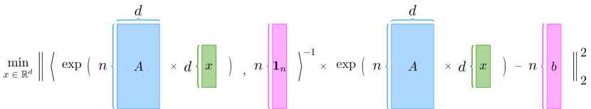
Figure 1: The visualization of the softmax regression (see Definition 1.1). $A$ is a matrix in $\mathbb{R}^{n\times d}$. $b,{\bf 1}_{n}\in\mathbb{R}^{n}$ and $x\in\mathbb{R}^{d}$ are vectors. First, we compute $\exp(Ax)$ by multiplying $A$ with $x$ and then calculating the exponential of each entry in their product. Second, we compute the inner product of $\exp(Ax)$ and ${\bf 1}_{n}$ and then find the multiplicative inverse of it. Third, we multiply the results of the first and the second step and subtract $b$ from it. Finally, we compute the minimum of the square of the $\ell_{2}$ norm of result of the third step. The blue rectangles represent the $n\times d$ matrices. The pink rectangles represent the $n$-dimensional vectors. The green rectangles represent the $d$-dimensional vectors.

Because of the explosive development of large language models (LLMs), there is an increasing amount of work focusing on the theoretical aspect of LLMs, aiming to improve the ability of LLMs from different aspects, including sentiment analysis [96], natural language translation [45], creative writing [67, 68], and language modeling [65]. One of the most important components of an LLM is its ability to identify and focus on the relevant information from the input text. Theoretical works [37, 60, 27, 16, 39, 34, 8, 106] analyze the attention computation to support this ability.

Definition 1.2 (Attention computation).

Let $Q$, $K$, and $V$ be $n\times d$ matrices whose entries are all real numbers.

Let $A=\exp(QK^{\top})$ and $D=\operatorname{diag}(A{\bf 1}_{n})$ be $n$-dimensional square matrices, where $\operatorname{diag}(A{\bf 1}_{n})$ is a diagonal matrix whose entries on the $i$-th row and $i$-th column is the same as the $i$-th entry of the vector $A{\bf 1}_{n}$.

The static attention computation is defined as

$$\mathsf{Att}(Q,K,V):=D^{-1}AV.$$

In attention computation, the matrix $Q$ is denoted as the query tokens, which are derived from the previous hidden state of decoders. $K$ and $V$ represent the key tokens and values. When computing $A$, the softmax function is applied to get the attention weight, namely $A_{i,j}$. Inspired by the role of the exponential functions in attention computation, prior research [34, 60] has built a theoretical framework of hyperbolic function regression, which includes the functions $f(x)=\exp(Ax),\cosh(Ax)$, and $\sinh(Ax)$.

Definition 1.3 (Hyperbolic regression, [60]).

Given a matrix $A\in\mathbb{R}^{n\times d}$ and a vector $b\in\mathbb{R}^{n}$, the goal of the hyperbolic regression problem is to compute the following regression problem:

$$\min_{x\in\mathbb{R}^{d}}\|f(x)-b\|_{2}.$$

The approach developed by [27] for analyzing the hyperbolic regression is to consider the normalization factor, namely $\langle f(x),{\bf 1}_{n}\rangle^{-1}=\langle\exp(Ax),{\bf 1}_{n}\rangle^{-1}$. By focusing on the $\exp$, [27] transform the hyperbolic regression problem (see Definition 1.3) to the softmax regression problem (see Definition 1.1). Later on, [59] studies the in-context learning based on a softmax regression of attention mechanism in the Transformer, which is an essential component within LLMs since it allows the model to focus on particular input elements. Moreover, [36] utilize a tensor-trick from [94, 105, 25, 85, 87, 28] simplifying the multiple softmax regression into a single softmax regression.

ResNet is a certain type of deep learning model: the weight layers can learn the residual functions [47]. It is characterized by skip connections, which may perform identity mappings by adding the layer’s output to the initial input. This mechanism is similar to the Highway Network in [82] that the gates are opened through highly positive bias weights. This innovation facilitates the training of deep learning models with a substantial number of layers, allowing them to achieve better accuracy as they become deeper. These identity skip connections, commonly known as “residual connections”, are also employed in various other systems, including Transformer [98], BERT [24], and ChatGPT [67]. Moreover, ResNets have achieved state-of-the-art performance across many computer vision tasks, including image classification [63, 83], object detection [70, 55, 57, 42], and semantic segmentation [33, 103, 99, 31]. Mathematically, it is defined as

$$Y_{j+1}=Y_{j}+F(Y_{j},\theta_{j})$$ (1)

where $Y_{j+1},Y_{j},F(Y_{j},\theta_{j})\in\mathbb{R}^{d}$: $Y_{j}$ represents the feature values at the $j$-th layer, while $\theta_{j}$ denotes the network parameters specific to that layer. The objective of the training process is to learn the network parameters $\theta$.

In this paper, we combine the softmax regression (see Definition 1.1) with ResNet and give a theoretical analysis of this problem. We formally define it as follows:

Definition 1.4 (Soft-Residual Regression).

Given a matrix $A\in\mathbb{R}^{n\times d}$ and a vector $b\in\mathbb{R}^{n}$, the goal is to compute the following regression problem:

$$\|\langle\exp(Ax)+Ax,{\bf 1}_{n}\rangle^{-1}(\exp(Ax)+Ax)-b\|_{2}^{2}$$

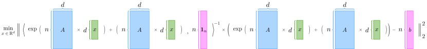
Figure 2: The visualization of the soft-residual regression (see Definition 1.4). $A$ is a matrix in $\mathbb{R}^{n\times d}$. $b,{\bf 1}_{n}\in\mathbb{R}^{n}$ and $x\in\mathbb{R}^{d}$ are vectors. First, we compute $\exp(Ax)$ by multiplying $A$ with $x$ and then calculating the exponential of each entry in their product. Second, we add $\exp(Ax)$ with $Ax$. Third, we compute the inner product of $\exp(Ax)+Ax$ and ${\bf 1}_{n}$ and then find the multiplicative inverse of it. Fourth, we multiply the results of the third step with $\exp(Ax)+Ax$ and subtract $b$ from it. Finally, we compute the minimum of the square of the $\ell_{2}$ norm of the result of the fourth step. The blue rectangles represent the $n\times d$ matrices. The pink rectangles represent the $n$-dimensional vectors. The green rectangles represent the $d$-dimensional vectors.

We are motivated by the fact that the softmax regression and ResNets have mostly been studied separately in prior works. We would like to provide a theoretical analysis for combining them together. The unified perspective and analysis of the loss landscape could provide insights into optimization and generalization for emerging overparametrized models. We firmly believe that this lays the groundwork for further research at the intersection of softmax classification and residual architectures.

Roadmap

In Section 2, we introduce the related work. In Section 3, we introduce the basic notations we use and present basic mathematical facts that may support the mathematical properties developed in this paper. In Section 4, we compute the gradient of the functions we defined earlier. In Section 5, we compute the Hessian of these functions based on their gradient. In Section 6, we formally define the key functions that appear in the Hessian and rewrite the Hessian functions in a more formal way. In Section 7, we show that the Hessian is positive semidefinite (PSD). In Section 8, we show that the Hessian is Lipschitz. In Section 9, we summarize the mathematical properties we developed in the previous sections and explain how they may support the main result of this paper. In Section 10, we conclude this paper, present the meaningfulness of our work, and discuss future research directions.

2 Related Work

In this section, we introduce the previous related research works.

Residual Neural Networks

ResNets were introduced by [47] for the purpose of simplifying the training of networks that are significantly deeper than those that were used previously. Its design is inspired by residual learning. [47] demonstrated state-of-the-art performance on image recognition benchmarks using extremely deep ResNets with over $100$ layers. By adding shortcut connections, ResNets were able to successfully train far deeper networks than previous architectures.

After being introduced, ResNets have become a prevalent research area in computer vision and its application. Many subsequent works were built based on the original ResNet model. In [102], ResNeXt is proposed: it splits each layer into smaller groups to increase the cardinality, which is defined as the size of the set of transformations. It is shown that the increase in cardinality leads to higher classification accuracy and is more effective than going deeper and wider when the capacity is increased. Moreover, [107] propose a novel architecture called wide residual networks (WRNs), and based on their experimental study, it is shown that residual networks with a reduced number of layers and an increased number of the network’s width are far superior to the thin and deep counterparts. In addition, ResNets is also studied with efficiency [46, 53, 78], video analysis [95, 71, 109, 1, 5], and breast cancer [97, 48, 4, 54, 64].

Moreover, ResNets has been found a connection with ordinary differential equations (ODEs). ResNets, as shown in Eq. (1), is a difference equation (or a discrete dynamical system). ODEs consider the continuous change of a dynamical system with respect to time. Therefore, a small parameter $h>0$ is introduced in Eq. (1), which makes this equation become continuous:

$$\frac{Y_{j+1}-Y_{j}}{h}=F(Y_{j},\theta_{j}),$$

which implies

$$\frac{\mathrm{d}Y(t)}{\mathrm{d}t}\approx F(Y(t),\theta(t)),~{}Y(0)=Y_{0}.$$

Due to the lack of general guidance to network architecture design, [62] connect the concept of ResNets with numerical differential equations, showing that ResNet can be interpreted as forward Euler discretizations of differential equations. Follow-up works expand this connection: [23] improves the accuracy by introducing more stable and adaptive ODE solvers for the use of ResNets, [44] establishes a new architecture based on ODEs to resolve the challenge of the vanishing gradient, and [22] construct a theoretical framework studying stability and reversibility of deep neural networks: there are three reversible neural network architectures that are developed, which theoretically can go arbitrary deep.

Attention

The attention matrix is a square matrix, which contains the associations between words or tokens in natural language text. Each row and column of an attention matrix align with the corresponding token, and the values within it signify the level of connection between these tokens. When generating the output, the attention matrix has a huge influence on determining the significance of individual input tokens within a sequence. Under this attention mechanism, each input token is assigned a weight or score that reflects its relevance with the current output generation.

There are various methods that have been developed to approximate the prominent entries of the attention matrix: methods like k-means clustering [26] and Locality Sensitive Hashing (LSH) [88, 20, 51] are to restrict the attention to nearby tokens, and other methods like [19] approximate the attention matrix by using the random feature maps based on Gaussian or exponential kernels. Furthermore, [17] presented that combining LSH-based and random feature-based methods is a more effective technique for estimating the attention matrix.

As presented in the recent works [37, 16, 106, 8, 34, 39, 60, 27] the calculation of inner product attention is a critical task. It is essential in training LLMs, like Transformer [98], GPT-1 [79], BERT [24], GPT-2 [81], GPT-3 [12], and ChatGPT, all of which have shown the extraordinary performance in handling natural language processing tasks, compared to smaller language models and traditional algorithms. Various studies have delved into different aspects of attention computation, such as softmax regression exploration [34, 27], exponential regression analysis [60], algorithms and complexity analysis for static attention computation [8], private computation of the attention matrix [37], and maintaining the attention matrix dynamically [16]. Additionally, there’s an algorithm for rescaled softmax regression [39], which presents an alternative formulation compared to exponential [60] and softmax regression methods [27]. [93] studies the attention kernel regression problem through the pre-conditioner. [35] studies the single layer of attention via the tensor and SVM tricks.

Softmax Regression

The softmax unit is a fundamental component of LLMs and serves a vital purpose: it enables the model to create a probability distribution concerning the possible following words or phrases when presented with a sequence of input words. Additionally, the softmax unit may allow the models to adapt their neural network’s weights and biases based on the available data. Under convex optimization, the softmax function is utilized for managing the progress and stability of potential functions, as shown in [15, 21]. Drawing inspiration from the concept of the softmax unit, [27] introduces a problem known as softmax regression. The studies study three particular formulations: exponential regression [34, 60], softmax regression [27, 59, 84, 101, 110], the rescaled softmax regression [39], and multiple softmax regression [36].

Convergence and Optimization

There are numerous studies analyzing the optimization and convergence to enhance training methods. [56] reveals that stochastic gradient descent may efficiently optimize over-parameterized neural networks for the structured data. Similarly, [32] shows that the gradient descent can also optimize over-parameterized neural networks. After that, [10] introduces a convergence theory for over-parameterized deep neural networks using gradient descent. Meanwhile, [11] investigates the rate at which training recurrent neural networks converge.

[2] gives an in-depth analysis of the optimization and generalization of over-parameterized two-layer neural networks. Moreover, [3] analyzes the exact computation using infinitely wide neural networks. On the other hand, [18] proposes the Gram-Gauss-Newton method, which is used to optimize over-parameterized neural networks.

In [104], global convergence of stochastic gradient descent is analyzed during the training of deep neural networks, which requires less over-parameterization compared to previous research. Furthermore, the works like [108, 50, 69] focus on the optimization and generalization aspects, whereas [60, 34] emphasize the convergence rate and stability.

Moreover, there are works such as [105, 6, 13, 66, 94] that concentrate on specialized optimization algorithms and techniques for training neural networks. Finally, [43, 58] centers their efforts on harnessing the structural aspects of neural networks for specific purposes.

In addition, there is a significant amount of work [90, 86, 85, 77, 80, 61, 73, 72, 76, 74, 75, 91, 30, 92, 38, 40] that analyze sketching: a technique to speed up machine learning algorithms and optimization.

3 Preliminary

In this section, we first introduce the basic notations we use. Then, in section 3.1, we introduce the definition of the functions we analyze in the later sections. In Section 3.2, we present the basic mathematical properties of the derivative, vectors, norms, and matrices.

Notations

Now, we define the notations used in this paper.

First, we define the notations related to sets. Let $\operatorname*{\mathbb{Z}}_{+}$ be the set containing all the positive integers, namely $\{1,2,3,\dots\}$. Let $n,d$ be arbitrary elements in $\operatorname*{\mathbb{Z}}_{+}$. We define $[n]:=\{1,2,\dots,n\}$. We define $\mathbb{R},\mathbb{R}^{n},\mathbb{R}^{n\times d}$ to be the set containing all real numbers, the set containing all $n$-dimensional vectors whose entries are all real numbers, and the set containing all $n\times d$ matrices whose entries are all real numbers, respectively.

Then, we define the notations related to vectors. Let $x,y$ be arbitrary elements in $\mathbb{R}^{n}$. We use $x_{i}$ to denote the $i$-th entry of $x$, for all $i\in[n]$. $\|x\|_{2}\in\mathbb{R}$ denotes the $\ell_{2}$ norm of the vector $x$, which is defined as $\|x\|_{2}:=(\sum_{i=1}^{n}x_{i}^{2})^{1/2}$. $\langle x,y\rangle\in\mathbb{R}$ represents the inner product of $x$ and $y$, which is defined as $\langle x,y\rangle:=\sum_{i=1}^{n}x_{i}y_{i}$. We use $\circ$ to denote a binary operation between $x$ and $y$, called the Hadamard product. $x\circ y\in\mathbb{R}^{n}$ is defined as $(x\circ y)_{i}:=x_{i}\cdot y_{i}$, for all $i\in[n]$. ${\bf 1}_{n}\in\mathbb{R}^{n}$ denotes a vector, where $({\bf 1}_{n})_{i}:=1$ for all $i\in[n]$, and ${\bf 0}_{n}\in\mathbb{R}^{n}$ denotes a vector, where $({\bf 0}_{n})_{i}:=0$ for all $i\in[n]$.

After that, we introduce the notations related to matrices. Let $A$ be an arbitrary element in $\mathbb{R}^{n\times d}$. We use $A_{i,j}$ to denote the entry of $A$ which is at the $i$-th row and $j$-th column, for all $i\in[n]$ and $j\in[d]$. We define $A_{*,i}\in\mathbb{R}^{n}$ as $(A_{*,i})_{j}:=A_{j,i}$, for all $j\in[n]$ and $i\in[d]$. We use $\|A\|$ to denote the spectral norm of $A$, i.e., $\|A\|:=\max_{x\in\mathbb{R}^{d}}\|Ax\|_{2}/\|x\|_{2}$. This also implies that for any $x\in\mathbb{R}^{d}$, $\|Ax\|_{2}\leq\|A\|\cdot\|x\|_{2}$. For any $x\in\mathbb{R}^{d}$, we define $\operatorname{diag}(x)\in\mathbb{R}^{d\times d}$ as $(\operatorname{diag}(x))_{i,j}:=x_{i}$ for all $i=j$ and $(\operatorname{diag}(x))_{i,j}:=0$ for all $i\neq j$, where $i,j\in[d]$. We use $A^{\top}\in\mathbb{R}^{d\times n}$ to denote the transpose of $A$, namely $(A^{\top})_{i,j}:=A_{j,i}$, for all $i\in[d]$ and $j\in[n]$. We use $I_{n}$ to denote the $n$-dimensional identity matrix. Let $B$ and $C$ be arbitrary symmetric matrices. We say $B\preceq C$ if, for all vector $x$, we have $x^{\top}Bx\leq x^{\top}Cx$. We say $B$ is positive semidefinite (or $B$ is a PSD matrix), denoted as $B\succeq 0$, if, for all vectors $x$, we have $x^{\top}Bx\geq 0$.

Finally, we define the notations related to functions. We define $\phi:\mathbb{R}\to\mathbb{R}$ as $\phi(z):=\max\{z,0\}$. For a differentiable function $f$, we use $\frac{\mathrm{d}f}{\mathrm{d}x}$ to denote the derivative of $f$.

3.1 Basic Definitions

In this section, we define the basic functions which are analyzed in the later sections.

Definition 3.1 (Basic functions).

Let $A\in\mathbb{R}^{n\times d}$ be an arbitrary matrix. Let $x\in\mathbb{R}^{d}$ be an arbitrary vector. Let $b\in\mathbb{R}^{n}$ be a given vector. Let $i\in[d]$ be an arbitrary positive integer. We define the functions $u_{1},u_{2},u,f,c,z,v_{i}:\mathbb{R}^{d}\to\mathbb{R}^{n}$ and $\alpha,L,\beta_{i}:\mathbb{R}^{d}\to\mathbb{R}$ as

$$u_{1}(x) :=Ax u_{2}(x) :=\exp(Ax)$$

$$u(x) :=u_{1}(x)+u_{2}(x) \alpha(x) :=\langle u(x),{\bf 1}_{n}\rangle$$

$$f(x) :=\alpha(x)^{-1}u(x) c(x) :=f(x)-b$$

$$L(x) :=0.5\|c(x)\|_{2}^{2} z(x) :=u_{2}(x)+{\bf 1}_{n}$$

$$v_{i}(x) :=(u_{2}(x)+{\bf 1}_{n})\circ A_{*,i} \beta_{i}(x) :=\langle v_{i}(x),{\bf 1}_{n}\rangle.$$

3.2 Basic Facts

In this section, we present the basic mathematical properties which are used to support our analysis in later sections.

Fact 3.2.

Let $f$ be a differentiable function. Then, we have

• Part 1. $\frac{\mathrm{d}}{\mathrm{d}x}\exp(x)=\exp(x)$

• Part 2. For any $j\neq i$, $\frac{\mathrm{d}}{\mathrm{d}x_{i}}f(x_{j})=0$

Fact 3.3.

For all vectors $u,v,w\in\mathbb{R}^{n}$, we have

• $\langle u,v\rangle=\langle u\circ v,{\bf 1}_{n}\rangle=u^{\top}\mathrm{diag}(v){\bf 1}_{n}$

• $\langle u\circ v,w\rangle=\langle u\circ w,v\rangle$

• $\langle u\circ v,w\rangle=\langle u\circ v\circ w,{\bf 1}_{n}\rangle=u^{\top}\operatorname{diag}(v)w$

• $\langle u\circ v\circ w\circ z,{\bf 1}_{n}\rangle=u^{\top}\operatorname{diag}(v\circ w)z$

• $u\circ v=v\circ u=\operatorname{diag}(u)\cdot v=\operatorname{diag}(v)\cdot u$

• $u^{\top}(v\circ w)=v^{\top}(u\circ w)=w^{\top}(u\circ v)=u^{\top}\operatorname{diag}(v)w=v^{\top}\operatorname{diag}(u)w=w^{\top}\operatorname{diag}(u)v$

• $\operatorname{diag}(u)\cdot\operatorname{diag}(v)\cdot{\bf 1}_{n}=\operatorname{diag}(u)v$

• $\operatorname{diag}(u\circ v)=\operatorname{diag}(u)\operatorname{diag}(v)$

• $\operatorname{diag}(u)+\operatorname{diag}(v)=\operatorname{diag}(u+v)$

• $\langle u,v\rangle=\langle v,u\rangle$

• $\langle u,v\rangle=u^{\top}v=v^{\top}u$

• $u+vw^{\top}a=u+vu^{\top}w=(I_{n}+vw^{\top})u$

• $u+v^{\top}wu=(1+v^{\top}w)u$

Fact 3.4.

Let $f:\mathbb{R}^{d}\to\mathbb{R}^{n}$. Let $q:\mathbb{R}^{d}\to\mathbb{R}$. Let $g:\mathbb{R}^{d}\rightarrow\mathbb{R}^{n}$. Therefore, we have for any arbitrary $x\in\mathbb{R}^{d}$, $q(x)\in\mathbb{R}$, $f(x)\in\mathbb{R}^{n}$, and $g(x)\in\mathbb{R}^{n}$. Let $a\in\mathbb{R}$ be an arbitrary constant.

Then, we have

• $\frac{\mathrm{d}q(x)^{a}}{\mathrm{d}x}=a\cdot q(x)^{a-1}\cdot\frac{\mathrm{d}q(x)}{\mathrm{d}x}$

• $\frac{\mathrm{d}\|f(x)\|^{2}_{2}}{\mathrm{d}t}=2\langle f(x),\frac{\mathrm{d}f(x)}{\mathrm{d}t}\rangle$

• $\frac{\mathrm{d}\langle f(x),g(x)\rangle}{\mathrm{d}t}=\langle\frac{\mathrm{d}f(x)}{\mathrm{d}t},g(x)\rangle+\langle f(x),\frac{\mathrm{d}g(x)}{\mathrm{d}t}\rangle$

• $\frac{\mathrm{d}(g(x)\circ f(x))}{\mathrm{d}t}=\frac{\mathrm{d}g(x)}{\mathrm{d}t}\circ f(x)+g(x)\circ\frac{\mathrm{d}f(x)}{\mathrm{d}t}$ (product rule for Hadamard product)

Fact 3.5 (Basic Vector Norm Bounds).

For vectors $u,v,w\in\mathbb{R}^{n}$, we have

• Part 1. $\langle u,v\rangle\leq\|u\|_{2}\cdot\|v\|_{2}$ (Cauchy-Schwarz inequality)

• Part 2. $\|\operatorname{diag}(u)\|\leq\|u\|_{\infty}$

• Part 3. $\|u\circ v\|_{2}\leq\|u\|_{\infty}\cdot\|v\|_{2}$

• Part 4. $\|u\|_{\infty}\leq\|u\|_{2}\leq\sqrt{n}\|u\|_{\infty}$

• Part 5. $\|u\|_{2}\leq\|u\|_{1}\leq\sqrt{n}\|u\|_{2}$

• Part 6. $\|\exp(u)\|_{\infty}\leq\exp(\|u\|_{\infty})\leq\exp(\|u\|_{2})$

• Part 7. Let $\alpha$ be a scalar, then $\|\alpha\cdot u\|_{2}=|\alpha|\cdot\|u\|_{2}$

• Part 8. $\|u+v\|_{2}\leq\|u\|_{2}+\|v\|_{2}$

• Part 9. $\|uv^{\top}\|\leq\|u\|_{2}\|v\|_{2}$

• Part 10. if $\|u\|_{2},\|v\|_{2}\leq R$, then $\|\exp(u)-\exp(v)\|_{2}\leq\exp(R)\|u-v\|_{2}$

Fact 3.6 (Matrices Norm Basics).

For any matrices $U,V\in\mathbb{R}^{n\times n}$, given a scalar $\alpha\in\mathbb{R}$ and a vector $v\in\mathbb{R}^{n}$, we have

• Part 1. $\|U^{\top}\|=\|U\|$

• Part 2. $\|U\|\geq\|V\|-\|U-V\|$

• Part 3. $\|U+V\|\leq\|U\|+\|V\|$

• Part 4. $\|U\cdot V\|\leq\|U\|\cdot\|V\|$

• Part 5. If $U\preceq\alpha\cdot V$, then $\|U\|\preceq\alpha\cdot\|V\|$

• Part 6. $\|\alpha\cdot U\|\leq|\alpha|\|U\|$

• Part 7. $\|Uv\|_{2}\leq\|U\|\cdot\|v\|_{2}$

• Part 8. $\|UU^{\top}\|\leq\|U\|^{2}$

Fact 3.7 (Basic algebraic properties).

Let $x$ be an arbitrary element in $\mathbb{R}$.

Then, we have

• Part 1. $\exp(x^{2})\geq 1$.

• Part 2. $\exp(x^{2})\geq x$.

Proof.

Proof of Part 1.

Consider

$$\frac{\mathrm{d}\exp(x^{2})}{\mathrm{d}x}=2x\exp(x^{2})=0.$$

This implies that

$$x=0$$

since

$$\exp(x^{2})\neq 0,\forall x\in\mathbb{R}.$$

Furthermore, since

$$\frac{\mathrm{d}\exp(x^{2})}{\mathrm{d}x}<0,\text{ when }x<0$$

and

$$\frac{\mathrm{d}\exp(x^{2})}{\mathrm{d}x}>0,\text{ when }x>0,$$

we have that

$$(0,\exp(0))$$

is the local minimum of $\exp(x^{2})$.

Since $x=0$ is the only critical point of $\exp(x^{2})$ and $\exp(x^{2})$ is differentiable over all $x\in\mathbb{R}$, so we have

$$\exp(x^{2})\geq\exp(0^{2})=1,$$

which completes the proof of the first part.

Proof of Part 2.

This strategy of proofing this part is the same as the first part by considering the derivative of $\exp(x^{2})-x$ and showing that the local minimum of $\exp(x^{2})-x$ is greater than $0$, so we omit the proof here. ∎

Fact 3.8.

For any vectors $u,v\in\mathbb{R}^{n}$, we have

• Part 1. $uu^{\top}\preceq\|u\|_{2}^{2}\cdot I_{n}$

• Part 2. $\operatorname{diag}(u)\preceq\|u\|_{2}\cdot I_{n}$

• Part 3. $\operatorname{diag}(u\circ u)\preceq\|u\|_{2}^{2}\cdot I_{n}$

• Part 4. $uv^{\top}+vu^{\top}\preceq uu^{\top}+vv^{\top}$

• Part 5. $uv^{\top}+vu^{\top}\succeq-(uu^{\top}+vv^{\top})$

• Part 6. $(v\circ u)(v\circ u)^{\top}\preceq\|v\|^{2}_{\infty}uu^{\top}$

• Part 7. $\operatorname{diag}(u\circ v)\preceq\|u\|_{2}\|v\|_{2}\cdot I_{n}$

4 Gradient

In this section, we compute the first-order derivatives of the functions defined earlier.

Lemma 4.1.

Let $x\in\mathbb{R}^{d}$ be an arbitrary vector. Let $u_{1}(x),u_{2}(x),u(x),f(x),c(x),z(x),v_{i}(x)\in\mathbb{R}^{n}$ be defined as in Definition 3.1. Let $\alpha(x),L(x),\beta_{i}(x)\in\mathbb{R}$ be defined as in Definition 3.1.

Then for each $i\in[d]$, we have

• Part 1. $\frac{\mathrm{d}u_{1}(x)}{\mathrm{d}x_{i}}=A_{*,i}$

• Part 2. $\frac{\mathrm{d}u_{2}(x)}{\mathrm{d}x_{i}}=u_{2}(x)\circ A_{*,i}$

• Part 3. $\frac{\mathrm{d}u(x)}{\mathrm{d}x_{i}}=v_{i}(x)$

• Part 4. $\frac{\mathrm{d}\alpha(x)}{\mathrm{d}x_{i}}=\beta_{i}(x)$

• Part 5. $\frac{\mathrm{d}\alpha(x)^{-1}}{\mathrm{d}x_{i}}=\alpha(x)^{-2}\cdot\beta_{i}(x)$

• Part 6. $\frac{\mathrm{d}f(x)}{\mathrm{d}x_{i}}=\alpha(x)^{-1}(I_{n}-f(x)\cdot{\bf 1}_{n}^{\top})\cdot v_{i}(x)$

• Part 7. $\frac{\mathrm{d}c(x)}{\mathrm{d}x_{i}}=\frac{\mathrm{d}f(x)}{\mathrm{d}x_{i}}=\alpha(x)^{-1}(I_{n}-f(x)\cdot{\bf 1}_{n}^{\top})\cdot v_{i}(x)$

• Part 8. $\frac{\mathrm{d}L(x)}{\mathrm{d}x_{i}}=\alpha(x)^{-1}c(x)^{\top}\cdot(I_{n}-f(x)\cdot{\bf 1}_{n}^{\top})\cdot v_{i}(x)$

  

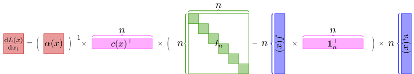
  Figure 3: The visualization of Part 8 of Lemma 4.1. We have $\alpha(x)\in\mathbb{R}$, $c(x),f(x),{\bf 1}_{n},v_{i}(x)\in\mathbb{R}^{n}$, and $I_{n}\in\mathbb{R}^{n\times n}$. First, we subtract the product of $f(x)$ and ${\bf 1}_{n}^{\top}$ from $I_{n}$. Then, we multiply the multiplicative inverse of $\alpha(x)$, $c(x)^{\top}$, the result from the first step, and $v_{i}(x)$, which gives us a scalar. The blue rectangles represent the $n$-dimensional vectors. The pink rectangles represent the transposes of $n$-dimensional vectors. The red squares represent the scalar. The green squares represent the identity matrix $I_{n}$.

• Part 9. $\frac{\mathrm{d}\beta_{i}(x)}{\mathrm{d}x_{i}}=\langle u_{2}(x),A_{*,i}\circ A_{*,i}\rangle$

• Part 10. For $j\in[d]\backslash\{i\}$, $\frac{\mathrm{d}\beta_{i}(x)}{\mathrm{d}x_{j}}=\langle u_{2}(x),A_{*,i}\circ A_{*,j}\rangle$

• Part 11. $\frac{\mathrm{d}v_{i}(x)}{\mathrm{d}x_{i}}=u_{2}(x)\circ A_{*,i}\circ A_{*,i}$

• Part 12. For $j\in[d]\backslash\{i\}$, $\frac{\mathrm{d}v_{i}(x)}{\mathrm{d}x_{j}}=u_{2}(x)\circ A_{*,j}\circ A_{*,i}$

Proof.

Proof of Part 1. For each $i\in[d]$, we have

$$\frac{\mathrm{d}Ax}{\mathrm{d}x_{i}}=~{} \frac{A\mathrm{d}x}{\mathrm{d}x_{i}}$$

$$=~{} A_{*,i}$$

where the first step follows from simple algebra and the last step follows from the fact that only the $i$-th entry of $\frac{\mathrm{d}x}{\mathrm{d}x_{i}}$ is $1$ and other entries of it are $0$.

Note that by definition 3.1,

$$u_{1}(x)=Ax.$$

Therefore, we have

$$\frac{\mathrm{d}u_{1}(x)}{\mathrm{d}x_{i}}=A_{*,i}.$$

Proof of Part 2. For each $i\in[d]$, we have

$$\frac{\mathrm{d}(u_{2}(x))_{i}}{\mathrm{d}x_{i}}= ~{}\frac{\mathrm{d}(\exp(Ax))_{i}}{\mathrm{d}x_{i}}$$

$$= ~{}\exp(Ax)_{i}\cdot\frac{\mathrm{d}(Ax)_{i}}{\mathrm{d}x_{i}}$$

$$= ~{}\exp(Ax)_{i}\cdot A_{*,i}$$

$$= ~{}(u_{2}(x))_{i}\cdot A_{*,i},$$

where the first step follows from the definition of $(u_{2}(x))_{i}$ (see Definition 3.1), the second step follows from Fact 3.2, the third step follows from Part 1, and the last step follows from the definition of $(u_{2}(x))_{i}$ (see Definition 3.1).

Thus, we have

$$\frac{\mathrm{d}u_{2}(x)}{\mathrm{d}x_{i}}=u_{2}(x)\circ A_{*,i}$$

Proof of Part 3.

We have

$$\frac{\mathrm{d}u(x)}{\mathrm{d}x_{i}}= ~{}\frac{\mathrm{d}(u_{1}(x)+u_{2}(x))}{\mathrm{d}x_{i}}$$

$$= ~{}\frac{\mathrm{d}(u_{1}(x))}{\mathrm{d}x_{i}}+\frac{\mathrm{d}(u_{2}(x))}{\mathrm{d}x_{i}}$$

$$= ~{}A_{*,i}+u_{2}(x)\circ A_{*,i}$$

$$= ~{}(u_{2}(x)+{\bf 1}_{n})\circ A_{*,i}$$

$$= ~{}v_{i}(x),$$

where the first step follows from the definition of $u(x)$ (see Definition 3.1), the second step follows from the basic derivative rule, the third step follows from results from Part 1 and Part 2, the fourth step follows from the basic properties of Hadamard product, and the last step follows from the definition of $v_{i}(x)$ (see Definition 3.1).

Proof of Part 4.

$$\frac{\mathrm{d}\alpha(x)}{\mathrm{d}x_{i}}= ~{}\frac{\mathrm{d}(\langle u(x),{\bf 1}_{n}\rangle)}{\mathrm{d}x_{i}}$$

$$= ~{}\langle\frac{\mathrm{d}u(x)}{\mathrm{d}x_{i}},{\bf 1}_{n}\rangle$$

$$= ~{}\langle v_{i}(x),{\bf 1}_{n}\rangle$$

$$= ~{}\beta_{i}(x)$$

where the first step follows from the definition of $\alpha(x)$ (see Definition 3.1), the second step follows from Fact 3.4, the third step follows from Part 3, and the fourth step follows from the definition of $\beta_{i}(x)$ (see Definition 3.1).

Proof of Part 5.

$$\frac{\mathrm{d}\alpha(x)^{-1}}{\mathrm{d}x_{i}}= ~{}-1\cdot\alpha(x)^{-2}\cdot\frac{\mathrm{d}\alpha(x)}{\mathrm{d}x_{i}}$$

$$= ~{}-\alpha(x)^{-2}\cdot\beta_{i}(x)$$

where the first step follows from the Fact 3.4, where the second step follows from the results of Part 4.

Proof of Part 6.

$$\frac{\mathrm{d}f(x)}{\mathrm{d}x_{i}}= ~{}\frac{\mathrm{d}\alpha(x)^{-1}}{\mathrm{d}x_{i}}u(x)+\alpha(x)^{-1}\cdot\frac{\mathrm{d}u(x)}{\mathrm{d}x_{i}}$$

$$= ~{}-\alpha(x)^{-2}\cdot\beta_{i}(x)\cdot u(x)+\alpha(x)^{-1}\cdot v_{i}(x)$$

$$= ~{}-\alpha(x)^{-1}f(x)\cdot\beta_{i}(x)+\alpha(x)^{-1}\cdot v_{i}(x)$$

$$= ~{}\alpha(x)^{-1}\cdot(v_{i}(x)-f(x)\cdot\beta_{i}(x))$$

$$= ~{}\alpha(x)^{-1}\cdot(v_{i}(x)-f(x)\cdot\langle v_{i}(x),{\bf 1}_{n}\rangle)$$

$$= ~{}\alpha(x)^{-1}\cdot(v_{i}(x)-f(x)\cdot{\bf 1}_{n}^{\top}v_{i}(x))$$

$$= ~{}\alpha(x)^{-1}\cdot(I_{n}-f(x)\cdot{\bf 1}_{n}^{\top})\cdot v_{i}(x)$$

where the first step follows from the product rule and the definition of $f(x)$ (see Definition 3.1), the second step follows from results of Part 3, 5, the third step follows from the definition of $f(x)$ (see Definition 3.1), the fourth step follows from simple algebra, the fifth step follows from the definition of $\beta_{i}$ (see Definition 3.1), the sixth step follows from Fact 3.3, and the last step follows from simple algebra.

Proof of Part 7.

$$\frac{\mathrm{d}c(x)}{\mathrm{d}x_{i}}= ~{}\frac{\mathrm{d}(f(x)-b)}{\mathrm{d}x_{i}}$$

$$= ~{}\frac{\mathrm{d}f(x)}{\mathrm{d}x_{i}}$$

where the first step follows from the definition of $c(x)$ (see Definition 3.1), the second step follows from derivative rules.

Proof of Part 8.

$$\frac{\mathrm{d}L(x)}{\mathrm{d}x_{i}}= ~{}\frac{\mathrm{d}0.5\|c(x)\|_{2}^{2}}{\mathrm{d}x_{i}}$$

$$= ~{}c(x)^{\top}\cdot\frac{\mathrm{d}c(x)}{\mathrm{d}x_{i}}$$

$$= ~{}\alpha(x)^{-1}\cdot c(x)^{\top}\cdot(I_{n}-f(x)\cdot{\bf 1}_{n}^{\top})\cdot v_{i}(x)$$

where the first step follows from the definition of $L(x)$ (see Definition 3.1), the second step follows from Fact 3.4, and the last step follows from the results from Part 6 and 7.

Proof of Part 9.

$$\frac{\mathrm{d}\beta_{i}(x)}{\mathrm{d}x_{i}}= ~{}\frac{\mathrm{d}(\langle v_{i}(x),{\bf 1}_{n}\rangle)}{\mathrm{d}x_{i}}$$

$$= ~{}\frac{\mathrm{d}(\langle(u_{2}(x)+{\bf 1}_{n})\circ A_{*,i},{\bf 1}_{n}\rangle)}{\mathrm{d}x_{i}}$$

$$= ~{}\frac{\mathrm{d}\langle u_{2}(x)+{\bf 1}_{n},A_{*,i}\rangle}{\mathrm{d}x_{i}}$$

$$= ~{}\langle\frac{\mathrm{d}(u_{2}(x)+{\bf 1}_{n})}{\mathrm{d}x_{i}},A_{*,i}\rangle$$

$$= ~{}\langle u_{2}(x)\circ A_{*,i},A_{*,i}\rangle$$

$$= ~{}\langle u_{2}(x),A_{*,i}\circ A_{*,i}\rangle$$

where the first step follows from the definition of $\beta_{i}(x)$ (see Definition 3.1), the second step follows from the definition of $v_{i}(x)$ (see Definition 3.1), the third step follows from Fact 3.3, the fourth step follows from Fact 3.4, the fifth step follows from Part 2, and the last step follows from Fact 3.3.

Proof of Part 10.

$$\frac{\mathrm{d}\beta_{i}(x)}{\mathrm{d}x_{j}}= ~{}\frac{\mathrm{d}(\langle v_{i}(x),{\bf 1}_{n}\rangle)}{\mathrm{d}x_{j}}$$

$$= ~{}\frac{\mathrm{d}(\langle(u_{2}(x)+{\bf 1}_{n})\circ A_{*,i},{\bf 1}_{n}\rangle)}{\mathrm{d}x_{j}}$$

$$= ~{}\frac{\mathrm{d}\langle u_{2}(x)+{\bf 1}_{n},A_{*,i}\rangle}{\mathrm{d}x_{j}}$$

$$= ~{}\langle\frac{\mathrm{d}(u_{2}(x)+{\bf 1}_{n})}{\mathrm{d}x_{j}},A_{*,i}\rangle$$

$$= ~{}\langle u_{2}(x)\circ A_{*,j},A_{*,i}\rangle$$

$$= ~{}\langle u_{2}(x),A_{*,j}\circ A_{*,i}\rangle$$

where the first step follows from the definition of $\beta_{i}(x)$ (see Definition 3.1), the second step follows from the definition of $v_{i}(x)$ (see Definition 3.1), the third step follows from Fact 3.3, the fourth step follows from Fact 3.4, the fifth step follows from Part 2, and the last step follows from Fact 3.3.

Proof of Part 11.

$$\frac{\mathrm{d}v_{i}(x)}{\mathrm{d}x_{i}}= ~{}\frac{\mathrm{d}(u_{2}(x)+{\bf 1}_{n})\circ A_{*,i}}{\mathrm{d}x_{i}}$$

$$= ~{}\frac{\mathrm{d}(u_{2}(x)+{\bf 1}_{n})}{\mathrm{d}x_{i}}\circ A_{*,i}$$

$$= ~{}u_{2}(x)\circ A_{*,i}\circ A_{*,i}$$

where the first step follows from the definition of $v_{i}(x)$ (see Definition 3.1), the second step follows from Fact 3.4 as $\frac{\mathrm{d}A_{*,i}}{\mathrm{d}x_{i}}=0$, and the last step follows from the results of Part 2.

Proof of Part 12.

$$\frac{\mathrm{d}v_{i}(x)}{\mathrm{d}x_{j}}= ~{}\frac{\mathrm{d}(u_{2}(x)+{\bf 1}_{n})\circ A_{*,i}}{\mathrm{d}x_{j}}$$

$$= ~{}\frac{\mathrm{d}(u_{2}(x)+{\bf 1}_{n})}{\mathrm{d}x_{j}}\circ A_{*,i}$$

$$= ~{}u_{2}(x)\circ A_{*,j}\circ A_{*,i}$$

where the first step follows from the definition of $v_{i}(x)$ (see Definition 3.1), the second step follows from Fact 3.4 as $\frac{\mathrm{d}A_{*,i}}{\mathrm{d}x_{j}}=0$, and the last step follows from the results of Part 2.

∎

5 Hessian

In Section 5.1, we introduce the basic definition of the matrices containing $B_{1}(x),B_{2}(x),B_{3}(x)\in\mathbb{R}^{n\times n}$, used for simplifying the expression of Hessian. In Section 5.2, we compute the second-order derivatives of the functions defined earlier. In Section 5.3, we present a helpful lemma. In Section 5.4, we decompose the matrices $B_{1}(x),B_{2}(x),B_{3}(x)\in\mathbb{R}^{n\times n}$ into low-rank matrices and diagonal matrices.

5.1 Basic Definition

In this section, we give the definition of the matrices containing $B_{1}(x),B_{2}(x),B_{3}(x)\in\mathbb{R}^{n\times n}$.

Definition 5.1.

Let $x\in\mathbb{R}^{d}$ be an arbitrary vector. Let $u_{1}(x),u_{2}(x),u(x),f(x),c(x),z(x),v_{i}(x)\in\mathbb{R}^{n}$ and $\alpha(x),L(x),\beta_{i}(x)\in\mathbb{R}$ be defined as in Definition 3.1. Let $K(x)=(I_{n}-f(x)\cdot{\bf 1}_{n}^{\top})\in\mathbb{R}^{n\times n}$. Let $\widetilde{c}(x)=K(x)^{\top}c(x)\in\mathbb{R}^{n}$. We define

• $B_{1}(x)\in\mathbb{R}^{n\times n}$ as

  $$~{}A_{*,i}^{\top}B_{1}(x)A_{*,j}$$

  $$:= ~{}\underbrace{\alpha(x)^{-2}}_{\mathrm{scalar}}\underbrace{v_{i}(x)^{\top}}_{1\times n}\underbrace{K(x)^{\top}}_{n\times n}\underbrace{K(x)}_{n\times n}\underbrace{v_{i}(x)}_{n\times 1}$$

• $B_{2}(x)\in\mathbb{R}^{n\times n}$ as

  $$~{}A_{*,i}^{\top}B_{2}(x)A_{*,j}$$

  $$:= ~{}-\underbrace{\alpha(x)^{-2}}_{\mathrm{scalar}}\cdot\underbrace{\widetilde{c}(x)^{\top}}_{1\times n}\cdot(\underbrace{v_{j}(x)}_{n\times 1}\cdot\underbrace{\beta_{i}(x)}_{\mathrm{scalar}}+\underbrace{v_{i}(x)\cdot\beta_{j}(x)}_{n\times 1})$$

• $B_{3}(x)\in\mathbb{R}^{n\times n}$ as

  $$A_{*,i}^{\top}B_{3}(x)A_{*,j}:=\underbrace{\alpha(x)^{-1}}_{\mathrm{scalar}}\cdot\underbrace{A_{*,i}^{\top}}_{1\times n}\mathrm{diag}(\underbrace{\widetilde{c}(x)}_{n\times 1}\circ\underbrace{u_{2}(x)}_{n\times 1})\underbrace{A_{*,j}}_{n\times 1}$$

5.2 Computation of Hessian

In this section, we present the computation of Hessian.

Lemma 5.2.

Let $x\in\mathbb{R}^{d}$ be an arbitrary vector. Let $u_{1}(x),u_{2}(x),u(x),f(x),c(x),z(x),v_{i}(x)\in\mathbb{R}^{n}$ and $\alpha(x),L(x),\beta_{i}(x)\in\mathbb{R}$ be defined as in Definition 3.1. Let $K(x)\in\mathbb{R}^{n\times n}$ and $\widetilde{c}(x)\in\mathbb{R}^{n}$ be defined as in Definition 5.1.

Then for each $i,j\in[d]$, and $j\neq i$, we have

• Part 1.

  $$\frac{\mathrm{d}^{2}u_{1}(x)}{\mathrm{d}x_{i}^{2}}={\bf 0}_{n}$$

• Part 2.

  $$\frac{\mathrm{d}^{2}u_{1}(x)}{\mathrm{d}x_{i}\mathrm{d}x_{j}}={\bf 0}_{n}$$

• Part 3.

  $$\frac{\mathrm{d}^{2}u_{2}(x)}{\mathrm{d}x_{i}^{2}}=A_{*,i}\circ u_{2}(x)\circ A_{*,i}$$

• Part 4.

  $$\frac{\mathrm{d}^{2}u_{2}(x)}{\mathrm{d}x_{i}\mathrm{d}x_{j}}=A_{*,i}\circ u_{2}(x)\circ A_{*,j}$$

• Part 5.

  $$\frac{\mathrm{d}^{2}u(x)}{\mathrm{d}x_{i}^{2}}=A_{*,i}\circ u_{2}(x)\circ A_{*,i}$$

• Part 6.

  $$\frac{\mathrm{d}^{2}u(x)}{\mathrm{d}x_{i}\mathrm{d}x_{j}}=A_{*,i}\circ u_{2}(x)\circ A_{*,j}$$

• Part 7.

  $$\frac{\mathrm{d}^{2}\alpha(x)}{\mathrm{d}x_{i}^{2}}=\langle u_{2}(x),A_{*,i}\circ A_{*,i}\rangle$$

• Part 8.

  $$\frac{\mathrm{d}^{2}\alpha(x)}{\mathrm{d}x_{i}\mathrm{d}x_{j}}=\langle u_{2}(x),A_{*,j}\circ A_{*,i}\rangle$$

• Part 9.

  $$\frac{\mathrm{d}^{2}\alpha(x)^{-1}}{\mathrm{d}x_{i}^{2}}=\underbrace{\alpha(x)^{-2}}_{\mathrm{scalar}}(\underbrace{\langle u_{2}(x),A_{*,i}\circ A_{*,i}\rangle}_{\mathrm{scalar}}-2\underbrace{\alpha(x)^{-1}\cdot\beta_{i}(x)^{2})}_{\mathrm{scalar}}$$

• Part 10.

  $$\frac{\mathrm{d}^{2}\alpha(x)^{-1}}{\mathrm{d}x_{i}\mathrm{d}x_{j}}=\underbrace{\alpha(x)^{-2}}_{\mathrm{scalar}}(\underbrace{\langle u_{2}(x),A_{*,i}\circ A_{*,j}\rangle}_{\mathrm{scalar}}-2\underbrace{\alpha(x)^{-1}\cdot\beta_{i}(x)\beta_{j}(x))}_{\mathrm{scalar}}$$

• Part 11.

  $$\frac{\mathrm{d}^{2}f(x)}{\mathrm{d}x_{i}^{2}}= ~{}-2\underbrace{\alpha(x)^{-2}}_{\mathrm{scalar}}\cdot\underbrace{\beta_{i}(x)}_{\mathrm{scalar}}\cdot\underbrace{(I_{n}-f(x)\cdot{\bf 1}_{n}^{\top})}_{n\times n}\cdot\underbrace{v_{i}(x)}_{n\times 1}+\underbrace{\alpha(x)^{-1}}_{\mathrm{scalar}}\cdot\underbrace{(I_{n}-f(x)\cdot{\bf 1}_{n}^{\top})}_{n\times n}\cdot\underbrace{(u_{2}(x)\circ A_{*,i}\circ A_{*,i})}_{n\times 1}$$

• Part 12.

  $$\frac{\mathrm{d}^{2}f(x)}{\mathrm{d}x_{i}\mathrm{d}x_{j}}= ~{}-\underbrace{\alpha(x)^{-2}}_{\mathrm{scalar}}\cdot\underbrace{(I_{n}-f(x)\cdot{\bf 1}_{n}^{\top})}_{n\times n}\cdot(\underbrace{v_{j}(x)}_{n\times 1}\cdot\underbrace{\beta_{i}(x)}_{\mathrm{scalar}}+\underbrace{v_{i}(x)}_{n\times 1}\cdot\underbrace{\beta_{j}(x)}_{\mathrm{scalar}})$$

  $$+ ~{}\underbrace{\alpha(x)^{-1}}_{\mathrm{scalar}}\underbrace{(I_{n}-f(x)\cdot{\bf 1}_{n}^{\top})}_{n\times n}\cdot\underbrace{(u_{2}(x)\circ A_{*,j}\circ A_{*,i})}_{n\times 1}$$

• Part 13.

  $$\frac{\mathrm{d}^{2}L(x)}{\mathrm{d}x_{i}^{2}}= ~{}\underbrace{\alpha(x)^{-2}}_{\mathrm{scalar}}\cdot\underbrace{A_{*,i}^{\top}}_{1\times n}\underbrace{B_{1}(x)}_{n\times n}\underbrace{A_{*,i}}_{n\times 1}-\underbrace{\alpha(x)^{-2}}_{\mathrm{scalar}}\cdot\underbrace{A_{*,i}^{\top}}_{1\times n}\underbrace{B_{2}(x)}_{n\times n}\underbrace{A_{*,i}}_{n\times 1}+\underbrace{\alpha(x)^{-1}}_{\mathrm{scalar}}\cdot\underbrace{A_{*,i}^{\top}}_{1\times n}\underbrace{B_{3}(x)}_{n\times n}\underbrace{A_{*,i}}_{n\times 1}$$

• Part 14.

  $$\frac{\mathrm{d}^{2}L(x)}{\mathrm{d}x_{i}\mathrm{d}x_{j}}= ~{}\underbrace{\alpha(x)^{-2}}_{\mathrm{scalar}}\cdot\underbrace{A_{*,i}^{\top}}_{1\times n}\underbrace{B_{1}(x)}_{n\times n}\underbrace{A_{*,j}}_{n\times 1}-\underbrace{\alpha(x)^{-2}}_{\mathrm{scalar}}\cdot\underbrace{A_{*,i}^{\top}}_{1\times n}\underbrace{B_{2}(x)}_{n\times n}\underbrace{A_{*,j}}_{n\times 1}+\underbrace{\alpha(x)^{-1}}_{\mathrm{scalar}}\cdot\underbrace{A_{*,i}^{\top}}_{1\times n}\underbrace{B_{3}(x)}_{n\times n}\underbrace{A_{*,j}}_{n\times 1}$$

Figure 4: The visualization of Part 14 of Lemma 5.2. We have $\alpha(x)\in\mathbb{R}$, $A_{*,i},A_{*,j}\in\mathbb{R}^{n}$, and $B_{1}(x),B_{2}(x),B_{3}(x)\in\mathbb{R}^{n\times n}$. First, we multiply $A_{*,i}^{\top}$ with $B_{1}(x)$, $B_{2}(x)$, $B_{3}(x)$, respectively, and use their product to multiply with $A_{*,j}$. Then, we use $\alpha(x)^{-2}$ to multiply with $A_{*,i}^{\top}B_{1}(x)A_{*,j}$ and with $A_{*,i}^{\top}B_{2}(x)A_{*,j}$, and we use $\alpha(x)^{-1}$ to multiply with $A_{*,i}^{\top}B_{3}(x)A_{*,j}$. Finally, we subtract $\alpha(x)^{-2}A_{*,i}^{\top}B_{2}(x)A_{*,j}$ from $\alpha(x)^{-2}A_{*,i}^{\top}B_{1}(x)A_{*,j}$, and we add this difference with $\alpha(x)^{-1}A_{*,i}^{\top}B_{3}(x)A_{*,j}$. The red squares represent scalars, the pink rectangles represent $1\times n$ matrices, the green squares represent the $n\times n$ squares, and the blue rectangles represent $n$-dimensional vectors.

Proof.

Proof of Part 1

$$\frac{\mathrm{d}^{2}u_{1}(x)}{\mathrm{d}x_{i}^{2}}= ~{}\frac{\mathrm{d}}{\mathrm{d}x_{i}}(\frac{\mathrm{d}u_{1}(x)}{\mathrm{d}x_{i}})$$

$$= ~{}\frac{\mathrm{d}A_{*,i}}{\mathrm{d}x_{i}}$$

$$= ~{}{\bf 0}_{n}$$

where the first step follows from the expansion of the Hessian, the second step follows from Part 1 of Lemma 4.1, and the last step follows from derivative rules.

Proof of Part 2

$$\frac{\mathrm{d}^{2}u_{1}(x)}{\mathrm{d}x_{i}\mathrm{d}x_{j}}= ~{}\frac{\mathrm{d}}{\mathrm{d}x_{j}}(\frac{\mathrm{d}u_{1}(x)}{\mathrm{d}x_{i}})$$

$$= ~{}\frac{\mathrm{d}A_{*,i}}{\mathrm{d}x_{j}}$$

$$= ~{}{\bf 0}_{n}$$

where the first step follows from the expansion of the Hessian, the second step follows from Part 1 of Lemma 4.1, and the last step follows from derivative rules.

Proof of Part 3

$$\frac{\mathrm{d}^{2}u_{2}(x)}{\mathrm{d}x_{i}^{2}}= ~{}\frac{\mathrm{d}}{\mathrm{d}x_{i}}(\frac{\mathrm{d}u_{2}(x)}{\mathrm{d}x_{i}})$$

$$= ~{}\frac{\mathrm{d}(u_{2}(x)\circ A_{*,i})}{\mathrm{d}x_{i}}$$

$$= ~{}A_{*,i}\circ\frac{\mathrm{d}u_{2}(x)}{\mathrm{d}x_{i}}$$

$$= ~{}A_{*,i}\circ u_{2}(x)\circ A_{*,i}$$

where the first step follows from the expansion of Hessian, the second step follows from Part 2 of Lemma 4.1, the third step follows from Fact 3.4, and the last step follows from Part 2 of Lemma 4.1.

Proof of Part 4

$$\frac{\mathrm{d}^{2}u_{2}(x)}{\mathrm{d}x_{i}x_{j}}= ~{}\frac{\mathrm{d}}{\mathrm{d}x_{j}}(\frac{\mathrm{d}u_{2}(x)}{\mathrm{d}x_{i}})$$

$$= ~{}\frac{\mathrm{d}(u_{2}(x)\circ A_{*,i})}{\mathrm{d}x_{j}}$$

$$= ~{}A_{*,i}\circ\frac{\mathrm{d}u_{2}(x)}{\mathrm{d}x_{j}}$$

$$= ~{}A_{*,i}\circ u_{2}(x)\circ A_{*,j}$$

where the first step follows from the expansion of Hessian, the second step follows from Part 2 of Lemma 4.1, the third step follows from Fact 3.4, and the last step follows from Part 2 of Lemma 4.1.

Proof of Part 5

$$\frac{\mathrm{d}^{2}u(x)}{\mathrm{d}x_{i}^{2}}= ~{}\frac{\mathrm{d}}{\mathrm{d}x_{i}}(\frac{\mathrm{d}u_{1}(x)+u_{2}(x)}{\mathrm{d}x_{i}})$$

$$= ~{}\frac{\mathrm{d}}{\mathrm{d}x_{i}}\frac{\mathrm{d}u_{1}(x)}{\mathrm{d}x_{i}}+\frac{\mathrm{d}}{\mathrm{d}x_{i}}\frac{\mathrm{d}u_{2}(x)}{\mathrm{d}x_{i}}$$

$$= ~{}A_{*,i}\circ u_{2}(x)\circ A_{*,i}$$

where the first step follows from the expansion of Hessian and Definition 3.1, the second step follows from the expansion of derivative, the third step follows from Part 1 and Part 3 of this Lemma.

Proof of Part 6

$$\frac{\mathrm{d}^{2}u(x)}{\mathrm{d}x_{i}x_{j}}= ~{}\frac{\mathrm{d}}{\mathrm{d}x_{j}}(\frac{\mathrm{d}u_{1}(x)+u_{2}(x)}{\mathrm{d}x_{i}})$$

$$= ~{}\frac{\mathrm{d}}{\mathrm{d}x_{j}}\frac{\mathrm{d}u_{1}(x)}{\mathrm{d}x_{i}}+\frac{\mathrm{d}}{\mathrm{d}x_{j}}\frac{\mathrm{d}u_{2}(x)}{\mathrm{d}x_{i}}$$

$$= ~{}A_{*,i}\circ u_{2}(x)\circ A_{*,j}$$

where the first step follows from the expansion of Hessian and Definition 3.1, the second step follows from the expansion of derivative, the third step follows from Part 2 and Part 4 of this Lemma.

Proof of Part 7

$$\frac{\mathrm{d}^{2}\alpha(x)}{\mathrm{d}x_{i}^{2}}= ~{}\frac{\mathrm{d}}{\mathrm{d}x_{i}}(\frac{\mathrm{d}\alpha(x)}{\mathrm{d}x_{i}})$$

$$= ~{}\frac{\mathrm{d}\beta_{i}(x)}{\mathrm{d}x_{i}}$$

$$= ~{}\langle u_{2}(x),A_{*,i}\circ A_{*,i}\rangle$$

where the first step follows from the expansion of Hessian, the second step follows from Part 4 of Lemma 4.1, and the last step follows from Part 9 of Lemma 4.1.

Proof of Part 8

$$\frac{\mathrm{d}^{2}\alpha(x)}{\mathrm{d}x_{i}x_{j}}= ~{}\frac{\mathrm{d}}{\mathrm{d}x_{j}}(\frac{\mathrm{d}\alpha(x)}{\mathrm{d}x_{i}})$$

$$= ~{}\frac{\mathrm{d}\beta_{i}(x)}{\mathrm{d}x_{j}}$$

$$= ~{}\langle u_{2}(x),A_{*,j}\circ A_{*,i}\rangle$$

where the first step follows from the expansion of Hessian, the second step follows from Part 4 of Lemma 4.1, and the last step follows from Part 10 of Lemma 4.1.

Proof of Part 9

$$\frac{\mathrm{d}^{2}\alpha(x)^{-1}}{\mathrm{d}x_{i}^{2}}= ~{}\frac{\mathrm{d}}{\mathrm{d}x_{i}}(\frac{\mathrm{d}\alpha(x)^{-1}}{\mathrm{d}x_{i}})$$

$$= ~{}\frac{\mathrm{d}(\alpha(x)^{-2}\cdot\beta_{i}(x))}{\mathrm{d}x_{i}}$$

$$= ~{}\frac{\mathrm{d}\alpha(x)^{-2}}{\mathrm{d}x_{i}}\cdot\beta_{i}(x)+\alpha(x)^{-2}\cdot\frac{\mathrm{d}\beta_{i}(x)}{\mathrm{d}x_{i}}$$

$$= ~{}-2\alpha(x)^{-3}\cdot\frac{\mathrm{d}\alpha(x)}{\mathrm{d}x_{i}}\cdot\beta_{i}(x)+\alpha(x)^{-2}\cdot\langle u_{2}(x),A_{*,i}\circ A_{*,i}\rangle$$

$$= ~{}-2\alpha(x)^{-3}\cdot\beta_{i}(x)^{2}+\alpha(x)^{-2}\cdot\langle u_{2}(x),A_{*,i}\circ A_{*,i}\rangle$$

$$= ~{}\alpha(x)^{-2}(\langle u_{2}(x),A_{*,i}\circ A_{*,i}\rangle-2\alpha(x)^{-1}\cdot\beta_{i}(x)^{2})$$

where the first step follows from the expansion of Hessian, the second step follows from Part 5 of Lemma 4.1, the third step follows from the product rule of derivative, the fourth step follows from Fact 3.4 and Part 9 of Lemma 4.1, the fifth step follows from Part 4 of Lemma 4.1, and the last step follows from simple algebra.

Proof of Part 10

$$\frac{\mathrm{d}^{2}\alpha(x)^{-1}}{\mathrm{d}x_{i}x_{j}}= ~{}\frac{\mathrm{d}}{\mathrm{d}x_{j}}(\frac{\mathrm{d}\alpha(x)^{-1}}{\mathrm{d}x_{i}})$$

$$= ~{}\frac{\mathrm{d}(\alpha(x)^{-2}\cdot\beta_{i}(x))}{\mathrm{d}x_{j}}$$

$$= ~{}\frac{\mathrm{d}\alpha(x)^{-2}}{\mathrm{d}x_{j}}\cdot\beta_{i}(x)+\alpha(x)^{-2}\cdot\frac{\mathrm{d}\beta_{i}(x)}{\mathrm{d}x_{j}}$$

$$= ~{}-2\alpha(x)^{-3}\cdot\frac{\mathrm{d}\alpha(x)}{\mathrm{d}x_{j}}\cdot\beta_{i}(x)+\alpha(x)^{-2}\cdot\langle u_{2}(x),A_{*,j}\circ A_{*,i}\rangle$$

$$= ~{}-2\alpha(x)^{-3}\cdot\beta_{i}(x)\cdot\beta_{j}(x)+\alpha(x)^{-2}\cdot\langle u_{2}(x),A_{*,j}\circ A_{*,i}\rangle$$

$$= ~{}\alpha(x)^{-2}(\langle u_{2}(x),A_{*,j}\circ A_{*,i}\rangle-2\alpha(x)^{-1}\cdot\beta_{i}(x)\cdot\beta_{j}(x))$$

where the first step follows from the expansion of Hessian, the second step follows from Part 5 of Lemma 4.1, the third step follows from the product rule of derivative, the fourth step follows from Fact 3.4 and Part 10 of Lemma 4.1, the fifth step follows from Part 4 of Lemma 4.1, and the last step follows from simple algebra.

Proof of Part 11

We first analyze the following equation:

$$\alpha(x)^{-1}\cdot(\frac{\mathrm{d}(I_{n}-f(x)\cdot{\bf 1}_{n}^{\top})}{\mathrm{d}x_{i}}\cdot v_{i}(x))= ~{}\alpha(x)^{-1}\cdot(\frac{\mathrm{d}I_{n}}{\mathrm{d}x_{i}}-\frac{\mathrm{d}f(x)\cdot{\bf 1}_{n}^{\top}}{\mathrm{d}x_{i}}\cdot v_{i}(x))$$

$$= ~{}\alpha(x)^{-1}\cdot(-\frac{\mathrm{d}f(x)}{\mathrm{d}x_{i}}\cdot{\bf 1}_{n}^{\top}\cdot v_{i}(x))$$

$$= ~{}\alpha(x)^{-1}\cdot(-\alpha(x)^{-1}(I_{n}-f(x)\cdot{\bf 1}_{n}^{\top})\cdot v_{i}(x)\cdot{\bf 1}_{n}^{\top}\cdot v_{i}(x))$$

$$= ~{}-\alpha(x)^{-2}\cdot(I_{n}-f(x)\cdot{\bf 1}_{n}^{\top})\cdot\beta_{i}(x)\cdot v_{i}(x),$$ (2)

where the first step follows from the basic derivative rule, the second step follows from the product rule, the third step follows from Part 6 of Lemma 4.1, and the last step follows from simple algebra and the definition of $\beta_{i}(x)$ (see Definition 3.1).

Then, we have

$$\frac{\mathrm{d}^{2}f(x)}{\mathrm{d}x_{i}^{2}}= ~{}\frac{\mathrm{d}}{\mathrm{d}x_{i}}(\frac{\mathrm{d}f(x)}{\mathrm{d}x_{i}})$$

$$= ~{}\frac{\mathrm{d}(\alpha(x)^{-1}\cdot(I_{n}-f(x)\cdot{\bf 1}_{n}^{\top})\cdot v_{i}(x))}{\mathrm{d}x_{i}}$$

$$= ~{}\frac{\mathrm{d}\alpha(x)^{-1}}{\mathrm{d}x_{i}}\cdot(I_{n}-f(x)\cdot{\bf 1}_{n}^{\top})\cdot v_{i}(x)+\alpha(x)^{-1}\cdot\frac{\mathrm{d}(I_{n}-f(x)\cdot{\bf 1}_{n}^{\top})\cdot v_{i}(x)}{\mathrm{d}x_{i}}$$

$$= ~{}-\alpha(x)^{-2}\cdot\beta_{i}(x)\cdot(I_{n}-f(x)\cdot{\bf 1}_{n}^{\top})\cdot v_{i}(x)$$

$$+ ~{}\alpha(x)^{-1}\cdot(\frac{\mathrm{d}(I_{n}-f(x)\cdot{\bf 1}_{n}^{\top})}{\mathrm{d}x_{i}}\cdot v_{i}(x)+(I_{n}-f(x)\cdot{\bf 1}_{n}^{\top})\cdot\frac{\mathrm{d}v_{i}(x)}{\mathrm{d}x_{i}})$$

$$= ~{}-\alpha(x)^{-2}\cdot\beta_{i}(x)\cdot(I_{n}-f(x)\cdot{\bf 1}_{n}^{\top})\cdot v_{i}(x)$$

$$+ ~{}-\alpha(x)^{-2}\cdot(I_{n}-f(x)\cdot{\bf 1}_{n}^{\top})\cdot v_{i}(x)\cdot\beta_{i}(x)+\alpha(x)^{-1}\cdot(I_{n}-f(x)\cdot{\bf 1}_{n}^{\top})\cdot(u_{2}(x)\circ A_{*,i}\circ A_{*,i})$$

$$= ~{}-2\alpha(x)^{-2}\cdot\beta_{i}(x)\cdot(I_{n}-f(x)\cdot{\bf 1}_{n}^{\top})\cdot v_{i}(x)+\alpha(x)^{-1}\cdot(I_{n}-f(x)\cdot{\bf 1}_{n}^{\top})\cdot(u_{2}(x)\circ A_{*,i}\circ A_{*,i})$$

where the first step follows from the expansion of Hessian, the second step follows from Part 6 of Lemma 4.1, the third step follows from the product rule of derivative, the fourth step follows from Part 5 of Lemma 4.1 and the product rule, the fifth step follows Eq. (5.2) and Part 11 of Lemma 4.1, and the last step follows from simple algebra.

Proof of Part 12

We first analyze the following equation:

$$\alpha(x)^{-1}\cdot(\frac{\mathrm{d}(I_{n}-f(x)\cdot{\bf 1}_{n}^{\top})}{\mathrm{d}x_{j}}\cdot v_{i}(x))= ~{}\alpha(x)^{-1}\cdot(\frac{\mathrm{d}I_{n}}{\mathrm{d}x_{j}}-\frac{\mathrm{d}f(x)\cdot{\bf 1}_{n}^{\top}}{\mathrm{d}x_{j}}\cdot v_{i}(x))$$

$$= ~{}\alpha(x)^{-1}\cdot(-\frac{\mathrm{d}f(x)}{\mathrm{d}x_{j}}\cdot{\bf 1}_{n}^{\top}\cdot v_{i}(x))$$

$$= ~{}\alpha(x)^{-1}\cdot(-\alpha(x)^{-1}(I_{n}-f(x)\cdot{\bf 1}_{n}^{\top})\cdot v_{j}(x)\cdot{\bf 1}_{n}^{\top}\cdot v_{i}(x))$$

$$= ~{}-\alpha(x)^{-2}\cdot(I_{n}-f(x)\cdot{\bf 1}_{n}^{\top})\cdot\beta_{i}(x)\cdot v_{j}(x),$$ (3)

where the first step follows from the basic derivative rule, the second step follows from the product rule, the third step follows from Part 6 of Lemma 4.1, and the last step follows from simple algebra and the definition of $\beta_{i}(x)$ (see Definition 3.1).

Then, we have

$$\frac{\mathrm{d}^{2}f(x)}{\mathrm{d}x_{i}x_{j}}= ~{}\frac{\mathrm{d}}{\mathrm{d}x_{j}}(\frac{\mathrm{d}f(x)}{\mathrm{d}x_{i}})$$

$$= ~{}\frac{\mathrm{d}(\alpha(x)^{-1}\cdot(I_{n}-f(x)\cdot{\bf 1}_{n}^{\top})\cdot v_{i}(x))}{\mathrm{d}x_{j}}$$

$$= ~{}\frac{\mathrm{d}\alpha(x)^{-1}}{\mathrm{d}x_{j}}\cdot(I_{n}-f(x)\cdot{\bf 1}_{n}^{\top})\cdot v_{i}(x)+\alpha(x)^{-1}\cdot\frac{\mathrm{d}(I_{n}-f(x)\cdot{\bf 1}_{n}^{\top})\cdot v_{i}(x))}{\mathrm{d}x_{j}}$$

$$= ~{}-\alpha(x)^{-2}\cdot\beta_{j}(x)\cdot(I_{n}-f(x)\cdot{\bf 1}_{n}^{\top})\cdot v_{i}(x)$$

$$+ ~{}\alpha(x)^{-1}\cdot(\frac{\mathrm{d}(I_{n}-f(x)\cdot{\bf 1}_{n}^{\top})}{\mathrm{d}x_{j}}\cdot v_{i}(x)+(I_{n}-f(x)\cdot{\bf 1}_{n}^{\top})\cdot\frac{\mathrm{d}v_{i}(x)}{\mathrm{d}x_{j}})$$

$$= ~{}-\alpha(x)^{-2}\cdot\beta_{j}(x)\cdot(I_{n}-f(x)\cdot{\bf 1}_{n}^{\top})\cdot v_{i}(x)$$

$$+ ~{}-\alpha(x)^{-2}\cdot(I_{n}-f(x)\cdot{\bf 1}_{n}^{\top})\cdot v_{j}(x)\cdot\beta_{i}(x)+\alpha(x)^{-1}\cdot(I_{n}-f(x)\cdot{\bf 1}_{n}^{\top})\cdot(u_{2}(x)\circ A_{*,j}\circ A_{*,i})$$

$$= ~{}-\alpha(x)^{-2}\cdot(I_{n}-f(x)\cdot{\bf 1}_{n}^{\top})\cdot(v_{j}(x)\cdot\beta_{i}(x)+v_{i}(x)\cdot\beta_{j}(x))$$

$$+ ~{}\alpha(x)^{-1}(I_{n}-f(x)\cdot{\bf 1}_{n}^{\top})\cdot(u_{2}(x)\circ A_{*,j}\circ A_{*,i})$$

where the first step follows from the expansion of Hessian, the second step follows from Part 6 of Lemma 4.1, the third step follows from the product rule of derivative, the fourth step follows from Part 5 of Lemma 4.1 and product rule, the fifth step follows from Eq. (5.2) and Part 12 of Lemma 4.1, and the last step follows from simple algebra.

Proof of Part 13

$$\frac{\mathrm{d}^{2}L(x)}{\mathrm{d}x_{i}^{2}}= ~{}\frac{\mathrm{d}}{\mathrm{d}x_{i}}(\frac{\mathrm{d}L(x)}{\mathrm{d}x_{i}})$$

$$= ~{}\frac{\mathrm{d}}{\mathrm{d}x_{i}}\langle c(x),\frac{\mathrm{d}c(x)}{\mathrm{d}x_{i}}\rangle$$

$$= ~{}\frac{\mathrm{d}}{\mathrm{d}x_{i}}\langle c(x),\frac{\mathrm{d}f(x)}{\mathrm{d}x_{i}}\rangle$$

$$= ~{}\langle\frac{\mathrm{d}c(x)}{\mathrm{d}x_{i}},\frac{\mathrm{d}f(x)}{\mathrm{d}x_{i}}\rangle+c(x)^{\top}\cdot\frac{\mathrm{d}^{2}f(x)}{\mathrm{d}^{2}x_{i}}$$

$$= ~{}(\alpha(x)^{-1}\cdot(I_{n}-f(x)\cdot{\bf 1}_{n}^{\top})\cdot v_{i}(x))^{\top}\cdot\alpha(x)^{-1}\cdot(I_{n}-f(x)\cdot{\bf 1}_{n}^{\top})\cdot v_{i}(x)$$

$$+ ~{}c(x)^{\top}\cdot-2\alpha(x)^{-2}\cdot\beta_{i}(x)\cdot(I_{n}-f(x)\cdot{\bf 1}_{n}^{\top})\cdot v_{i}(x)$$

$$+ ~{}\alpha(x)^{-1}\cdot c(x)^{\top}\cdot(I_{n}-f(x)\cdot{\bf 1}_{n}^{\top})\cdot(u_{2}(x)\circ A_{*,i}\circ A_{*,i})$$

$$= ~{}\alpha(x)^{-2}v_{i}(x)^{\top}K(x)^{\top}K(x)v_{i}(x)$$

$$+ ~{}-2\alpha(x)^{-2}\cdot\widetilde{c}(x)^{\top}\cdot v_{i}(x)\cdot\beta_{i}(x)$$

$$+ ~{}\alpha(x)^{-1}\cdot A_{*,i}^{\top}\mathrm{diag}(\widetilde{c}(x)\circ u_{2}(x))A_{*,i}$$

$$= ~{}A_{*,i}^{\top}B_{1}(x)A_{*,i}+A_{*,i}^{\top}B_{2}(x)A_{*,i}+A_{*,i}^{\top}B_{3}(x)A_{*,i}$$

where the first step follows from the expansion of Hessian, the second step follows from Fact 3.4, the third step follows from Part 7 of Lemma 4.1, the fourth step follows from Fact 3.4, the fifth step follows from Part 7 of Lemma 4.1 and Part 11 of Lemma 5.2, the sixth step follows from Definition of $\widetilde{c},K$ (See Definition 5.1), and the last step follow from Definitions of $B_{1},B_{2},B_{3}$ (See Definition 5.1).

Proof of Part 14

$$\frac{\mathrm{d}^{2}L(x)}{\mathrm{d}x_{i}x_{j}}= ~{}\frac{\mathrm{d}}{\mathrm{d}x_{j}}(\frac{\mathrm{d}L(x)}{\mathrm{d}x_{i}})$$

$$= ~{}\frac{\mathrm{d}}{\mathrm{d}x_{j}}\langle c(x),\frac{\mathrm{d}c(x)}{\mathrm{d}x_{i}}\rangle$$

$$= ~{}\frac{\mathrm{d}}{\mathrm{d}x_{j}}\langle c(x),\frac{\mathrm{d}f(x)}{\mathrm{d}x_{i}}\rangle$$

$$= ~{}\frac{\mathrm{d}c(x)^{\top}}{\mathrm{d}x_{j}}\cdot\frac{\mathrm{d}f(x)}{\mathrm{d}x_{i}}+c(x)^{\top}\cdot\frac{\mathrm{d}^{2}f(x)}{\mathrm{d}x_{i}x_{j}}$$

$$= ~{}(\alpha(x)^{-1}\cdot(I_{n}-f(x)\cdot{\bf 1}_{n}^{\top})\cdot v_{j}(x))^{\top}\cdot\alpha(x)^{-1}\cdot(I_{n}-f(x)\cdot{\bf 1}_{n}^{\top})\cdot v_{i}(x)$$

$$+ ~{}c(x)^{\top}\cdot(-\alpha(x)^{-2}\cdot(I_{n}-f(x)\cdot{\bf 1}_{n}^{\top})\cdot(v_{j}(x)\cdot\beta_{i}(x)+v_{i}(x)\cdot\beta_{j}(x))$$

$$+ ~{}\alpha(x)^{-1}(I_{n}-f(x)\cdot{\bf 1}_{n}^{\top})\cdot(u_{2}(x)\circ A_{*,j}\circ A_{*,i}))$$

$$= ~{}\alpha(x)^{-2}v_{i}(x)^{\top}K(x)^{\top}K(x)v_{j}(x)$$

$$+ ~{}-\alpha(x)^{-2}\cdot\widetilde{c}(x)^{\top}\cdot(v_{j}(x)\cdot\beta_{i}(x)+v_{i}(x)\cdot\beta_{j}(x))$$

$$+ ~{}\alpha(x)^{-1}\cdot A_{*,i}^{\top}\mathrm{diag}(\widetilde{c}(x)\circ u_{2}(x))A_{*,j}$$

$$= ~{}A_{*,i}^{\top}B_{1}(x)A_{*,j}+A_{*,i}^{\top}B_{2}(x)A_{*,j}+A_{*,i}^{\top}B_{3}(x)A_{*,j}$$

where the first step follows from the expansion of Hessian, the second step follows from Fact 3.4, the third step follows from Part 7 of Lemma 4.1, the fourth step follows from Fact 3.4, the fifth step follows from Part 7 of Lemma 4.1 and Part 12 of Lemma 5.2, the sixth step follows from Definition of $\widetilde{c},K$ (See Definition 5.1), and the last step follow from Definitions of $B_{1},B_{2},B_{3}$ (See Definition 5.1). ∎

5.3 Helpful Lemma

In this section, we present a helpful lemma that is used for further analysis of Hessian.

Lemma 5.3.

Let $x\in\mathbb{R}^{d}$ be an arbitrary vector. Let $u_{1}(x),u_{2}(x),u(x),f(x),c(x),z(x),v_{i}(x)\in\mathbb{R}^{n}$ and $\alpha(x),L(x),\beta_{i}(x)\in\mathbb{R}$ be defined as in Definition 3.1. Let $K(x)\in\mathbb{R}^{n\times n}$ and $\widetilde{c}(x)\in\mathbb{R}^{n}$ be defined as in Definition 5.1.

Then, for each $i,j\in[d]$,

• Part 1.

  $$~{}\alpha(x)^{-2}\cdot v_{i}(x)^{\top}K(x)^{\top}K(x)v_{j}(x)$$

  $$= ~{}\underbrace{A_{*,i}^{\top}}_{1\times n}\cdot\underbrace{\alpha(x)^{-2}}_{\mathrm{scalar}}\cdot\underbrace{\operatorname{diag}(z(x))}_{n\times n}$$

  $$\cdot ~{}\underbrace{K(x)^{\top}}_{n\times n}\underbrace{K(x)}_{n\times n}\cdot\operatorname{diag}(\underbrace{z(x)}_{n\times 1})\cdot\underbrace{A_{*,j}}_{n\times 1}$$

• Part 2.

  $$~{}\alpha(x)^{-2}\cdot\widetilde{c}(x)^{\top}\cdot(v_{j}(x)\cdot\beta_{i}(x)+v_{i}(x)\cdot\beta_{j}(x))$$

  $$= ~{}\underbrace{A_{*,i}^{\top}}_{1\times n}\cdot\underbrace{\alpha(x)^{-2}}_{\mathrm{scalar}}\cdot\underbrace{z(x)}_{n\times 1}\cdot\underbrace{\widetilde{c}(x)^{\top}}_{1\times n}\cdot\underbrace{\operatorname{diag}(z(x))}_{n\times n}\cdot\underbrace{A_{*,j}}_{n\times 1}$$

  $$+ ~{}\underbrace{A_{*,i}^{\top}}_{1\times n}\cdot\underbrace{\alpha(x)^{-2}}_{\mathrm{scalar}}\cdot\underbrace{\operatorname{diag}(z(x))}_{n\times n}\cdot\underbrace{\widetilde{c}(x)}_{n\times 1}\cdot\underbrace{z(x)^{\top}}_{1\times n}\cdot\underbrace{A_{*,j}}_{n\times 1}$$

• Part 3.

  $$~{}\alpha(x)^{-1}\cdot A_{*,i}^{\top}\mathrm{diag}(\widetilde{c}(x)\circ u_{2}(x))A_{*,j}$$

  $$= ~{}\underbrace{A_{*,i}^{\top}}_{1\times n}\cdot\underbrace{\alpha(x)^{-1}}_{\mathrm{scalar}}\cdot\underbrace{\mathrm{diag}(\widetilde{c}(x)\circ u_{2}(x))}_{n\times n}\underbrace{A_{*,j}}_{n\times 1}$$

Proof.

Proof of Part 1.

$$~{}\alpha(x)^{-2}\cdot v_{i}(x)^{\top}K(x)^{\top}K(x)v_{j}(x)$$

$$= ~{}\alpha(x)^{-2}\cdot((z(x)\circ A_{*,i})^{\top}\cdot K(x)^{\top}K(x)\cdot(z(x)\circ A_{*,j}))$$

$$= ~{}\alpha(x)^{-2}\cdot(\operatorname{diag}(z(x))\cdot A_{*,i})^{\top}\cdot K(x)^{\top}K(x)\cdot\operatorname{diag}(z(x))\cdot A_{*,j}$$

$$= ~{}A_{*,i}^{\top}\cdot\alpha(x)^{-2}\cdot\operatorname{diag}(z(x))\cdot K(x)^{\top}K(x)\cdot\operatorname{diag}(z(x))\cdot A_{*,j}$$

where the first step follows from the definition of $v_{i}(x)$ (see Definition 3.1), the second step follows from Fact 3.3, and the last step follows from simple algebra and the definition of $z(x)$ (see Definition 3.1).

Proof of Part 2.

$$~{}\alpha(x)^{-2}\cdot\widetilde{c}(x)^{\top}\cdot(v_{j}(x)\cdot\beta_{i}(x)+v_{i}(x)\cdot\beta_{j}(x))$$

$$= ~{}\alpha(x)^{-2}\cdot\widetilde{c}(x)^{\top}\cdot z(x)\circ A_{*,j}\cdot\langle z(x),A_{*,i}\rangle$$

$$+ ~{}\alpha(x)^{-2}\cdot\widetilde{c}(x)^{\top}\cdot z(x)\circ A_{*,i}\cdot\langle z(x),A_{*,j}\rangle$$

$$= ~{}\alpha(x)^{-2}\cdot\widetilde{c}(x)^{\top}\operatorname{diag}(z(x))\cdot A_{*,j}\cdot z(x)^{\top}\cdot A_{*,i}$$

$$+ ~{}\alpha(x)^{-2}\cdot\widetilde{c}(x)^{\top}\operatorname{diag}(z(x))\cdot A_{*,i}\cdot z(x)^{\top}\cdot A_{*,j}$$

$$= ~{}(A_{*,j}^{\top}\cdot\alpha(x)^{-2}\cdot\operatorname{diag}(z(x))\cdot\widetilde{c}(x)\cdot z(x)^{\top}\cdot A_{*,i})^{\top}$$

$$+ ~{}A_{*,i}^{\top}\cdot\alpha(x)^{-2}\cdot\operatorname{diag}(z(x))\cdot\widetilde{c}(x)\cdot(z(x))^{\top}\cdot A_{*,j}$$

$$= ~{}A_{*,i}^{\top}\cdot\alpha(x)^{-2}\cdot z(x)\cdot\widetilde{c}(x)^{\top}\cdot\operatorname{diag}(z(x))\cdot A_{*,j}$$

$$+ ~{}A_{*,i}^{\top}\cdot\alpha(x)^{-2}\cdot\operatorname{diag}(z(x))\cdot\widetilde{c}(x)\cdot z(x)^{\top}\cdot A_{*,j}$$

where the first step follows from the definition of $\beta_{i}(x)$ and $v_{i}(x)$ (see Definition 3.1), the second step follows from Fact 3.3, the third step follows from Fact 3.3, and the last step follows from simple algebra and the definition of $z(x)$ (see Definition 3.1).

Proof of Part 3.

$$~{}\alpha(x)^{-1}\cdot A_{*,i}^{\top}\mathrm{diag}(\widetilde{c}(x)\circ u_{2}(x))A_{*,i}$$

$$= ~{}A_{*,i}^{\top}\cdot\alpha(x)^{-1}\cdot\mathrm{diag}(\widetilde{c}(x)\circ u_{2}(x))A_{*,i}$$

where the first step follows from the simple algebra.

∎

5.4 Decomposing $B_{1}(x),B_{2}(x)$ and $B_{3}(x)$ into low rank plus diagonal

In this section, we decompose the matrices $B_{1}(x)$, $B_{2}(x)$, and $B_{3}(x)$ into low rank plus diagonal.

Lemma 5.4.

Let $x\in\mathbb{R}^{d}$ be an arbitrary vector. Let $u_{1}(x),u_{2}(x),u(x),f(x),c(x),z(x),v_{i}(x)\in\mathbb{R}^{n}$ and $\alpha(x),L(x),\beta_{i}(x)\in\mathbb{R}$ be defined as in Definition 3.1. Let $K(x),B_{1}(x),B_{2}(x),B_{3}(x)\in\mathbb{R}^{n\times n}$ and $\widetilde{c}(x)\in\mathbb{R}^{n}$ be defined as in Definition 5.1 and $B(x)=B_{1}(x)+B_{2}(x)+B_{3}(x)\in\mathbb{R}^{n\times n}$.

Then, we show that

• Part 1. For $B_{1}(x)\in\mathbb{R}^{n\times n}$, we have

  $$B_{1}(x)=\underbrace{\alpha(x)^{-2}}_{\mathrm{scalar}}\cdot\underbrace{\operatorname{diag}(z(x))}_{n\times n}\cdot\underbrace{K(x)^{\top}}_{n\times n}\underbrace{K(x)}_{n\times n}\cdot\operatorname{diag}(\underbrace{z(x)}_{n\times 1})$$

• Part 2. For $B_{2}(x)\in\mathbb{R}^{n\times n}$, we have

  $$B_{2}(x)= ~{}-\underbrace{\alpha(x)^{-2}}_{\mathrm{scalar}}\cdot\underbrace{\widetilde{c}(x)}_{n\times 1}\cdot\underbrace{z(x)^{\top}}_{1\times n}\cdot\underbrace{\operatorname{diag}(z(x))}_{n\times n}$$

  $$- ~{}\underbrace{\alpha(x)^{-2}}_{\mathrm{scalar}}\cdot\underbrace{\operatorname{diag}(z(x))}_{n\times n}\cdot\underbrace{z(x)}_{n\times 1}\cdot\underbrace{\widetilde{c}(x)^{\top}}_{1\times n}$$

• Part 3. For $B_{3}(x)\in\mathbb{R}^{n\times n}$, we have

  $$B_{3}(x)=\underbrace{\alpha(x)^{-1}}_{\mathrm{scalar}}\cdot\mathrm{diag}(\underbrace{\widetilde{c}(x)}_{n\times 1}\circ\underbrace{u_{2}(x)}_{n\times 1})$$

• Part 4. For $B(x)\in\mathbb{R}^{n\times n}$, we have

  $$B(x)= ~{}\underbrace{\alpha(x)^{-2}}_{\mathrm{scalar}}\underbrace{\operatorname{diag}(z(x))}_{n\times n}\cdot\underbrace{K(x)^{\top}}_{n\times n}\underbrace{K(x)}_{n\times n}\cdot\operatorname{diag}(\underbrace{z(x)}_{n\times 1})$$

  $$- ~{}\underbrace{\alpha(x)^{-2}}_{\mathrm{scalar}}\cdot\underbrace{\widetilde{c}(x)}_{n\times 1}\cdot\underbrace{z(x)^{\top}}_{1\times n}\cdot\underbrace{\operatorname{diag}(z(x))}_{n\times n}$$

  $$- ~{}\underbrace{\alpha(x)^{-2}}_{\mathrm{scalar}}\cdot\underbrace{\operatorname{diag}(z(x))}_{n\times n}\cdot\underbrace{z(x)}_{n\times 1}\cdot\underbrace{\widetilde{c}(x)^{\top}}_{1\times n}$$

  $$+ ~{}\underbrace{\alpha(x)^{-1}}_{\mathrm{scalar}}\cdot\mathrm{diag}(\underbrace{\widetilde{c}(x)}_{n\times 1}\circ\underbrace{u_{2}(x)}_{n\times 1})$$

Proof.

Proof of Part 1

$$A_{*,i}^{\top}B_{1}(x)A_{*,j}= ~{}\underbrace{\alpha(x)^{-2}}_{\mathrm{scalar}}\cdot\underbrace{v_{i}(x)^{\top}}_{1\times n}\underbrace{K(x)^{\top}}_{n\times n}\underbrace{K(x)}_{n\times n}\underbrace{v_{i}(x)}_{n\times 1}$$

$$= ~{}A_{*,i}^{\top}\cdot\alpha(x)^{-2}\cdot\operatorname{diag}(z(x))^{\top}\cdot K(x)^{\top}K(x)\cdot\operatorname{diag}(z(x))\cdot A_{*,j}$$

where the first step follows from Definition 5.1, and the last step follows from Lemma 5.3.

Thus, by extracting $A_{*,i}^{\top}$ and $A_{*,j}$, we get:

$$B_{1}(x)=\alpha(x)^{-2}\cdot\operatorname{diag}(z(x))^{\top}\cdot K(x)^{\top}K(x)\cdot\operatorname{diag}(z(x))$$

Proof of Part 2.

$$~{}A_{*,i}^{\top}B_{2}(x)A_{*,j}$$

$$= ~{}-\alpha(x)^{-2}\cdot\widetilde{c}(x)^{\top}\cdot(v_{j}(x)\cdot\beta_{i}(x)+v_{i}(x)\cdot\beta_{j}(x))$$

$$= ~{}-(A_{*,i}^{\top}\cdot\alpha(x)^{-2}\cdot z(x)\cdot\widetilde{c}(x)^{\top}\cdot\operatorname{diag}(z(x))\cdot A_{*,j}$$

$$+ ~{}A_{*,i}^{\top}\cdot\alpha(x)^{-2}\cdot\operatorname{diag}(z(x))\cdot\widetilde{c}(x)\cdot z(x)^{\top}\cdot A_{*,j})$$

where the first step follows from the Definition of $A_{*,i}^{\top}B_{2}(x)A_{*,j}$ (see Definition 5.1), and the last step follows from Lemma 5.3.

Thus, by extracting $A_{*,i}^{\top}$ and $A_{*,j}$, we get:

$$B_{2}(x)= ~{}-(\alpha(x)^{-2}\cdot z(x)\cdot\widetilde{c}(x)^{\top}\cdot\operatorname{diag}(z(x))$$

$$+ ~{}\alpha(x)^{-2}\cdot\operatorname{diag}(z(x))\cdot\widetilde{c}(x)\cdot z(x)^{\top})$$

Proof of Part 3.

$$A_{*,i}^{\top}B_{3}(x)A_{*,j}= ~{}A_{*,i}^{\top}\cdot\alpha(x)^{-1}\cdot\mathrm{diag}(\widetilde{c}(x)\circ u_{2}(x))A_{*,j}$$

where the first step follows from Lemma 5.3.

Thus, by extracting $A_{*,i}^{\top}$ and $A_{*,j}$, we get:

$$B_{3}(x)=\alpha(x)^{-1}\cdot\mathrm{diag}(\widetilde{c}(x)\circ u_{2}(x))$$

Proof of Part 4.

Since $B(x)=B_{1}(x)+B_{2}(x)+B_{3}(x)$, by combining the first three part, we can get $B(x)$.

∎

6 Rewrite Hessian

In this section, we rewrite the hessian. For convenience of analysis, we formally make a definition block for $B(x)$.

Definition 6.1.

Let $x\in\mathbb{R}^{d}$ be an arbitrary vector. Let $u_{1}(x),u_{2}(x),u(x),f(x),c(x),z(x),v_{i}(x)\in\mathbb{R}^{n}$ and $\alpha(x),L(x),\beta_{i}(x)\in\mathbb{R}$ be defined as in Definition 3.1. Let $K(x)\in\mathbb{R}^{n\times n}$ and $\widetilde{c}(x)\in\mathbb{R}^{n}$ be defined as in Definition 5.1.

Then, we define $B(x)\in\mathbb{R}^{n\times n}$ as follows:

$$B(x):= ~{}\alpha(x)^{-2}\cdot\operatorname{diag}(z(x))\cdot K(x)^{\top}K(x)\cdot\operatorname{diag}(z(x))$$

$$- ~{}\alpha(x)^{-2}\cdot z(x)\cdot\widetilde{c}(x)^{\top}\cdot\operatorname{diag}(z(x))-\alpha(x)^{-2}$$

$$\cdot ~{}\operatorname{diag}(z(x))\cdot\widetilde{c}(x)\cdot z(x)^{\top}$$

$$+ ~{}\alpha(x)^{-1}\cdot\mathrm{diag}(\widetilde{c}(x)\circ u_{2}(x)).$$

Furthermore, we defined $B_{\operatorname{mat}}(x),B_{\operatorname{rank}}(x),B_{\operatorname{diag}}(x)\in\mathbb{R}^{n\times n}$ as follows:

$$B_{\operatorname{mat}}(x):= ~{}\alpha(x)^{-2}\cdot\operatorname{diag}(z(x))\cdot K(x)^{\top}K(x)\cdot\operatorname{diag}(z(x))$$

$$B_{\operatorname{rank}}(x):= ~{}\alpha(x)^{-2}\cdot(z(x)\cdot\widetilde{c}(x)^{\top}\cdot\operatorname{diag}(z(x))$$

$$+ ~{}\operatorname{diag}(z(x))\cdot\widetilde{c}(x)\cdot z(x)^{\top})$$

$$B_{\operatorname{diag}}(x):= ~{}\alpha(x)^{-1}\cdot\operatorname{diag}(\widetilde{c}(x)\circ u_{2}(x)),$$

so that

$$B(x)=B_{\operatorname{mat}}(x)-B_{\operatorname{rank}}(x)+B_{\operatorname{diag}}(x).$$

7 Hessian is PSD

In this section, we mainly prove Lemma 7.1.

7.1 PSD Lower Bound

Lemma 7.1.

Let $x\in\mathbb{R}^{d}$ be an arbitrary vector. Let $u_{1}(x),u_{2}(x),u(x),f(x),c(x),z(x),v_{i}(x)\in\mathbb{R}^{n}$ and $\alpha(x),L(x),\beta_{i}(x)\in\mathbb{R}$ be defined as in Definition 3.1. Let $K(x),B(x),B_{\operatorname{mat}}(x),B_{\operatorname{rank}}(x),B_{\operatorname{diag}}(x)\in\mathbb{R}^{n\times n}$ and $\widetilde{c}(x)\in\mathbb{R}^{n}$ be defined as in Definition 6.1. Let $\beta\in(0,0.1)$ and $\beta<\alpha(x)$.

Then, we have

• Part 1.

  $$0\preceq B_{\operatorname{mat}}(x)\preceq\beta^{-2}\cdot 16n^{2}\exp(2R^{2})\cdot I_{n}$$

• Part 2.

  $$-10\beta^{-2}n\exp(R^{2})\cdot I_{n}\preceq-B_{\operatorname{rank}}(x)\preceq 10\beta^{-2}n\exp(R^{2})\cdot I_{n}$$

• Part 3.

  $$-4\beta^{-1}n\exp(R^{2})\cdot I_{n}\preceq B_{\operatorname{diag}}(x)\preceq 4\beta^{-1}n\exp(R^{2})\cdot I_{n}$$

• Part 4.

  $$-14\beta^{-2}n\exp(R^{2})\cdot I_{n}\preceq B(x)\preceq 30\beta^{-2}n^{2}\exp(2R^{2})\cdot I_{n}$$

Proof.

Proof of Part 1.

On the one hand,

$$B_{\operatorname{mat}}= ~{}\alpha(x)^{-2}\cdot\operatorname{diag}(z(x))\cdot K(x)^{\top}K(x)\cdot\operatorname{diag}(z(x))$$

$$\preceq ~{}\alpha(x)^{-2}\|\operatorname{diag}(z(x))K(x)^{\top}\|^{2}\cdot I_{n}$$

$$\preceq ~{}\alpha(x)^{-2}\|\operatorname{diag}(z(x))\|^{2}\|K(x)^{\top}\|^{2}\cdot I_{n}$$

$$\preceq ~{}\alpha(x)^{-2}\|z(x)\|_{2}^{2}\cdot 4n\cdot I_{n}$$

$$\preceq ~{}\beta^{-2}\cdot 16n^{2}\exp(2R^{2})\cdot I_{n}$$

where the first step follows from definition of $B_{\operatorname{mat}}$, the second step follows from Part 1 of Fact 3.8, the third step follows from Part 4 of Fact 3.6, the fourth step follows from Part 2,4 of Fact 3.5 and Part 7 of Lemma 8.2, and the final step follows from Part 8 of Lemma 8.2 and $\alpha(x)>\beta$.

On the other hand, since $B_{\operatorname{mat}}$ is a positive semi-definite matrix, then $B_{\operatorname{mat}}\succeq 0$.

Proof of Part 2

On the one hand

$$B_{\operatorname{rank}}(x)= ~{}\alpha(x)^{-2}\cdot z(x)\cdot\widetilde{c}(x)^{\top}\cdot\operatorname{diag}(z(x))$$

$$+ ~{}\alpha(x)^{-2}\cdot\operatorname{diag}(z(x))\cdot\widetilde{c}(x)\cdot z(x)^{\top}$$

$$\preceq ~{}\alpha(x)^{-2}\cdot(z(x)z(x)^{\top}$$

$$+ ~{}\widetilde{c}(x)^{\top}\cdot\operatorname{diag}(z(x))\cdot(\widetilde{c}(x)^{\top}\cdot\operatorname{diag}(z(x)))^{\top})$$

$$\preceq ~{}\alpha(x)^{-2}(\|z(x)\|_{2}^{2}+\|\widetilde{c}(x)^{\top}\operatorname{diag}(z(x))\|_{2}^{2})\cdot I_{n}$$

$$\preceq ~{}\alpha(x)^{-2}(2\sqrt{n}\exp(R^{2})+\|\widetilde{c}(x)\|_{2}^{2}\|z(x)\|_{2}^{2})\cdot I_{n}$$

$$\preceq ~{}\alpha(x)^{-2}(2\sqrt{n}\exp(R^{2})+8n\exp(R^{2}))\cdot I_{n}$$

$$\preceq ~{}10\beta^{-2}n\exp(R^{2})\cdot I_{n}$$

where the first step follows from the definition of $B_{\operatorname{rank}}(x)$, the second step follows from Part 4 of Fact 3.8, the third step follows from Part 1 of Fact 3.8, the fourth step follows from Part 8 of Lemma 8.2 and Part 9 of Fact 3.5, the fifth step follows from Part 8, 10 of Lemma 8.2, and the last step follows from $n>1$ and $\alpha(x)>\beta$.

Then, by multiplying $-1$ on both sides, we can get

$$-B_{\operatorname{rank}}(x)\succeq-10\beta^{-2}n\exp(R^{2})\cdot I_{n}$$

On the other hand, the proof of the lower bound is similar to the previous one, so we omit it here.

Proof of Part 3

On the one hand

$$B_{\operatorname{diag}}(x)= ~{}\alpha(x)^{-1}\cdot\operatorname{diag}(\widetilde{c}(x)\circ u_{2}(x))$$

$$\preceq ~{}\alpha(x)^{-1}\|\widetilde{c}(x)\|_{2}\|u_{2}(x)\|_{2}\cdot I_{n}$$

$$\preceq ~{}4\beta^{-1}n\exp(R^{2})\cdot I_{n}$$

where the first step follows from the definition of $B_{\operatorname{diag}}(x)$, the second step follows from Part 7 of Fact 3.8, and the last step follows from Part 1, 10 of Lemma 8.2 and $\alpha(x)>\beta$.

On the other hand, the proof of the lower bound is similar to the previous one, so we omit it here.

Proof of Part 4

On the one hand

$$B(x)= ~{}B_{\operatorname{mat}}(x)-B_{\operatorname{rank}}(x)+B_{\operatorname{diag}}(x)$$

$$\preceq ~{}\beta^{-2}\cdot 16n^{2}\exp(2R^{2})\cdot I_{n}+10\beta^{-2}n\exp(R^{2})\cdot I_{n}$$

$$+ ~{}4\beta^{-1}n\exp(R^{2})\cdot I_{n}$$

$$\preceq ~{}30\beta^{-2}n^{2}\exp(2R^{2})\cdot I_{n}$$

where the first step follows from Definition 6.1, the second step follows Part 1, 2, 3, and the last step follows from $\beta^{-1}>1,n>1$, and $\exp(2R^{2})>\exp(R^{2})$.

On the other hand, we have

$$B(x)= ~{}B_{\operatorname{mat}}(x)-B_{\operatorname{rank}}(x)+B_{\operatorname{diag}}(x)$$

$$\succeq ~{}-10\beta^{-2}n\exp(R^{2})\cdot I_{n}-4\beta^{-1}n\exp(R^{2})\cdot I_{n})$$

$$\succeq ~{}-14\beta^{-2}n\exp(R^{2})\cdot I_{n}$$

where the first step follows from Definition 6.1, the second step follows Part 1, 2, 3, and the last step follows from $\beta^{-1}>1$. ∎

8 Hessian is Lipschitz

In this section, we find the upper bound of $\|\nabla^{2}L(x)-\nabla^{2}L(y)\|$ and thus proved that $\nabla^{2}L$ is Lipschitz. More specifically, in section 8.1, we give a summary of the main properties developed in this whole section. In Section 8.2, we present the upper bound of the norms of the functions we analyzed before. In Section 8.3, we present the Lipschitz properties of the functions we analyzed before. In Section 8.4, we summarize the four steps of the Lipschitz for matrix functions. In Section 8.5, we analyze the first step of the Lipschitz for matrix function $\alpha(x)^{-2}\cdot\operatorname{diag}(z(x))^{\top}\cdot K(x)^{\top}K(x)\cdot\operatorname{diag}(z(x))$. In Section 8.6, we analyze the second step of the Lipschitz for matrix function $\alpha(x)^{-2}\cdot z(x)\cdot\widetilde{c}(x)^{\top}\cdot\operatorname{diag}(z(x))$. In Section 8.7, we analyze the third step of the Lipschitz for matrix function $\alpha(x)^{-2}\cdot\operatorname{diag}(z(x))\cdot\widetilde{c}(x)\cdot z(x)^{\top}$. In Section 8.8, we analyze the fourth step of the Lipschitz for matrix function $\alpha(x)^{-1}\cdot\mathrm{diag}(\widetilde{c}(x)\circ u_{2}(x))$.

8.1 Main results

In this section, we present the main lemma which is the summary of the properties developed in this whole section.

Lemma 8.1.

Let $H(x)=\frac{\mathrm{d}^{2}L}{\mathrm{d}x^{2}}$.

Then we have

$$\|H(x)-H(y)\|\leq 20\beta^{-5}n^{3.5}\exp(8R^{2})\|x-y\|_{2}$$

Proof.

The definition of $G_{i}$ is as follows

• $G_{1}(x)=\alpha(x)^{-2}\cdot\operatorname{diag}(z(x))\cdot K(x)^{\top}K(x)\cdot\operatorname{diag}(z(x))$

• $G_{2}(x)=-\alpha(x)^{-2}\cdot z(x)\cdot\widetilde{c}(x)^{\top}\cdot\operatorname{diag}(z(x))$

• $G_{3}(x)=-\alpha(x)^{-2}\cdot\operatorname{diag}(z(x))\cdot\widetilde{c}(x)\cdot z(x)^{\top}$

• $G_{4}(x)=\alpha(x)^{-1}\cdot\mathrm{diag}(\widetilde{c}(x)\circ u_{2}(x))$,

which we define and analyze in Lemma 8.5, 8.6, 8.7, 8.8, respectively.

Then, we have

$$\|H(x)-H(y)\|= ~{}\|A\|\|\sum_{i=1}^{4}G_{i}(x)-G_{i}(y)\|\|A\|$$

$$\leq ~{}R^{2}\cdot\|\sum_{i=1}^{4}G_{i}(x)-G_{i}(y)\|$$

$$\leq ~{}R^{2}\cdot 20\beta^{-5}n^{3.5}\exp(7R^{2})\|x-y\|_{2}$$

$$\leq ~{}20\beta^{-5}n^{3.5}\exp(8R^{2})\|x-y\|_{2}$$

where the first step follows from the definition of $G_{i}$ (see Lemma 8.4) and matrix spectral norm, the second step follows from $\|A\|\leq R$, the second step follows from Lemma 8.4, and the last step follows from $R^{2}\leq\exp(R^{2})$ ∎

8.2 A core Tool: Upper Bound for Several Basic Functions

In this section, we find the upper bound for the norms of the functions we analyze.

Lemma 8.2.

Let $R\geq 4$. Let $A\in\mathbb{R}^{n\times d}$ and $x\in\mathbb{R}^{d}$ satisfy $\|A\|\leq R$ and $\|x\|_{2}\leq R$. Let $b\in\mathbb{R}^{n}$ satisfy $\|b\|_{1}\leq 1$. Let $u_{1}(x),u_{2}(x),u(x),f(x),c(x),z(x),v_{i}(x)\in\mathbb{R}^{n}$ and $\alpha(x),L(x),\beta_{i}(x)\in\mathbb{R}$ be defined as in Definition 3.1. Let $K(x),B(x),B_{\operatorname{mat}}(x),B_{\operatorname{rank}}(x),B_{\operatorname{diag}}(x)\in\mathbb{R}^{n\times n}$ and $\widetilde{c}(x)\in\mathbb{R}^{n}$ be defined as in Definition 6.1. Let $\beta\in(0,0.1)$, and $\langle\exp(Ax),{\bf 1}_{n}\rangle$, $\langle\exp(Ay),{\bf 1}_{n}\rangle$, $\langle\exp(Ax)+Ax,{\bf 1}_{n}\rangle$, and $\langle\exp(Ay)+Ay,{\bf 1}_{n}\rangle$ be greater than or equal to $\beta$, respectively. Let $R_{f}=2\beta^{-1}\cdot(R\exp(R^{2})+R)\cdot(n\cdot\exp(R^{2})+\sqrt{n}\cdot R^{2})$. We define $R_{f,2}\in\mathbb{R}$ as $R_{f,2}:=2\sqrt{n}\beta^{-1}\exp(R^{2})$.

Then, we have

• Part 1. $\|\exp(Ax)\|_{2}\leq\sqrt{n}\exp(R^{2})$

• Part 2. $\|\exp(Ax)+Ax\|_{2}\leq 2\sqrt{n}\exp(R^{2})$

• Part 3. $|\alpha(x)|\geq\beta$

• Part 4. $|\alpha(x)^{-1}|\leq\beta^{-1}$

• Part 5. $\|f(x)\|_{2}\leq R_{f,2}$

• Part 6. $\|c(x)\|_{2}\leq 2R_{f,2}$

• Part 7. $\|K(x)\|\leq 3\sqrt{n}\cdot R_{f,2}$

• Part 8 $\|z(x)\|_{2}\leq 2\sqrt{n}\cdot\exp(R^{2})$

• Part 9 $|\alpha(x)^{-2}|\leq\beta^{-2}$

• Part 10 $\|\widetilde{c}(x)\|_{2}\leq 10\sqrt{n}R_{f,2}^{2}$

Proof.

Proof of Part 1

$$\|\exp(Ax)\|_{2}\leq ~{}\sqrt{n}\cdot\|\exp(Ax)\|_{\infty}$$

$$\leq ~{}\sqrt{n}\cdot\exp(\|(Ax)\|_{\infty})$$

$$\leq ~{}\sqrt{n}\cdot\exp(\|(Ax)\|_{2})$$

$$\leq ~{}\sqrt{n}\cdot\exp(R^{2})$$

where the first step follows from Fact 3.5, the second step follows from Part 6 of Fact 3.5, the third step follows from Part 6 of Fact 3.5, and the last step follows from $\|A\|\leq R$ and $\|x\|_{2}\leq R$.

Proof of Part 2

$$\|\exp(Ax)+Ax\|_{2}\leq ~{}\|\exp(Ax)\|_{2}+\|Ax\|_{2}$$

$$\leq ~{}\sqrt{n}\cdot\exp(R^{2})+R^{2}$$

$$\leq ~{}2\sqrt{n}\exp(R^{2})$$

where the first step follows from Part 8 of Fact 3.5, the second step follows from Part 1 and $\|A\|\leq R,\|x\|_{2}\leq R$, and the last step follows from $n>1,\exp(R^{2})\geq R^{2}$.

Proof of Part 3

$$|\alpha(x)|= ~{}|\langle u(x),{\bf 1}_{n}\rangle|$$

$$\geq ~{}|\langle\exp(Ax)+Ax,{\bf 1}_{n}\rangle|$$

$$\geq ~{}\beta$$

where the first step follows from the definition of $\alpha(x)$ (see Definition 3.1), the second step follows the definition of $u(x)$ (see Definition 3.1), and the last step follows from the assumption $\langle\exp(Ax)+Ax,{\bf 1}_{n}\rangle\geq\beta$.

Proof of Part 4

We have

$$|\alpha(x)^{-1}|\leq ~{}|\beta^{-1}|$$

$$\leq ~{}\beta^{-1}$$

where the first step follows from Part 3 of Lemma 8.2, the second step follows from $\beta^{-1}>0$.

Proof of Part 5

First, we analyze the following equation:

$$|\langle\exp(Ax)+Ax,{\bf 1}_{n}\rangle^{-1}|= ~{}|\langle\exp(Ax)+Ax,{\bf 1}_{n}\rangle|^{-1}$$

$$\leq ~{}\beta^{-1},$$ (4)

where the first step follows from simple algebra and the second step follows from the assumption in the Lemma statement.

Then, we have

$$\|f(x)\|_{2}= ~{}\|\alpha(x)^{-1}u(x)\|_{2}$$

$$= ~{}\|\langle\exp(Ax)+Ax,{\bf 1}_{n}\rangle^{-1}(\exp(Ax)+Ax)\|_{2}$$

$$= ~{}|\langle\exp(Ax)+Ax,{\bf 1}_{n}\rangle^{-1}|\cdot\|(\exp(Ax)+Ax)\|_{2}$$

$$\leq ~{}\beta^{-1}\cdot\|(\exp(Ax)+Ax)\|_{2}$$

$$\leq ~{}2\sqrt{n}\beta^{-1}\exp(R^{2})$$

$$= ~{}R_{f,2},$$

where the first step follows from the definition of $f(x)$ (see Definition 3.1), the second step follows from the definition of $\alpha(x)$ and $u(x)$ (see Definition 3.1), the third step follows from Fact 3.5, the fourth step follows from Eq. (8.2), and the fifth step follows from Part 2, and the last step follows from the definition of $R_{f,2}$.

Proof of Part 6

$$\|c(x)\|_{2}= ~{}\|f(x)-b\|_{2}$$

$$\leq ~{}\|f(x)\|_{2}+\|b\|_{2}$$

$$\leq ~{}R_{f,2}+1$$

$$\leq ~{}2R_{f,2},$$

where the first step follows from the definition of $c(x)$ (see Definition 3.1), the second step follows from Part 8 of Fact 3.5, the third step follows from Part 5 of Lemma 8.2 and $\|b\|_{2}\leq\|b\|_{1}\leq 1$, and the last step follows from $R_{f,2}\geq 1$.

Proof of Part 7

$$\|K(x)\|= ~{}\|(I_{n}-f(x)\cdot{\bf 1}_{n}^{\top})\|$$

$$\leq ~{}\|I_{n}\|+\|f(x)\cdot{\bf 1}_{n}^{\top}\|$$

$$\leq ~{}1+\|f(x)\|_{2}\cdot\|{\bf 1}_{n}^{\top}\|_{2}$$

$$\leq ~{}1+2\sqrt{n}\beta^{-1}\exp(R^{2})\cdot\sqrt{n}$$

$$\leq ~{}3\sqrt{n}R_{f,2},$$

where the first step follows from the definition of $K(x)$, the second step follows from the Part 3 of Fact 3.6, the third step follows from $\|I_{n}\|=1$ and Part 9 of Fact 3.5, and the fourth step follows from Part 5 of Lemma 8.2, and the last step follows from the simple algebra.

Proof of Part 8

$$\|z(x)\|_{2}= ~{}\|u_{2}(x)+{\bf 1}_{n}\|$$

$$\leq ~{}\|u_{2}(x)\|_{2}+\|{\bf 1}_{n}\|_{2}$$

$$\leq ~{}\sqrt{n}\cdot(\exp(R^{2})+1)$$

$$\leq ~{}2\sqrt{n}\exp(R^{2})$$

where the first step follows from the the definition of $z(x)$ (see Definition 3.1), the second step follows from Part 8 of Fact 3.5, the third step follows from Part 1 of Lemma 8.2, and the last step follows from Fact 3.7.

Proof of Part 9

$$|\alpha(x)^{-2}|= ~{}|\alpha(x)^{-1}|^{2}$$

$$\leq ~{}\beta^{-2}$$

where the first step follows from simple algebra, and the last step follows from Part 4 of Lemma 8.2.

Proof of Part 10

$$\|\widetilde{c}(x)\|_{2}= ~{}\|K(x)^{\top}c(x)\|_{2}$$

$$\leq ~{}\|K(x)\|\|c(x)\|_{2}$$

$$\leq ~{}3\sqrt{n}R_{f,2}\cdot 2R_{f,2}$$

$$\leq ~{}10\sqrt{n}R_{f,2}^{2},$$

where the first step follows from Definition of $\widetilde{c}(x)$, the second step follows from Part 7 of Fact 3.6, the third step follows from Part 6 and 7 of Lemma 8.2, and the last step follows from simple algebra. ∎

8.3 A core Tool: Lipschitz Property for Several Basic Functions

In this section, we present the Lipschitz property for the functions we analyze.

Lemma 8.3 (Basic Functions Lipschitz Property).

Let $R\geq 4$. Let $A\in\mathbb{R}^{n\times d}$ and $x\in\mathbb{R}^{d}$ satisfy $\|A\|\leq R$ and $\|x\|_{2}\leq R$. Let $b\in\mathbb{R}^{n}$ satisfy $\|b\|_{1}\leq 1$. Let $u_{1}(x),u_{2}(x),u(x),f(x),c(x),z(x),v_{i}(x)\in\mathbb{R}^{n}$ and $\alpha(x),L(x),\beta_{i}(x)\in\mathbb{R}$ be defined as in Definition 3.1. Let $K(x),B(x),B_{\operatorname{mat}}(x),B_{\operatorname{rank}}(x),B_{\operatorname{diag}}(x)\in\mathbb{R}^{n\times n}$ and $\widetilde{c}(x)\in\mathbb{R}^{n}$ be defined as in Definition 6.1. Let $\beta\in(0,0.1)$, and $\langle\exp(Ax),{\bf 1}_{n}\rangle$, $\langle\exp(Ay),{\bf 1}_{n}\rangle$, $\langle\exp(Ax)+Ax,{\bf 1}_{n}\rangle$, and $\langle\exp(Ay)+Ay,{\bf 1}_{n}\rangle$ be greater than or equal to $\beta$, respectively. Let $R_{f}=6\beta^{-2}\cdot n\cdot\exp(3R^{2})$.

Then, we have

• Part 1. $\|Ax-Ay\|_{2}\leq R\cdot\|x-y\|_{2}$

• Part 2. $\|\exp(Ax)-\exp(Ay)\|_{2}\leq R\exp(R^{2})\cdot\|x-y\|_{2}$

• Part 3. $|\alpha(x)-\alpha(y)|\leq 2\sqrt{n}R\exp(R^{2})\|x-y\|_{2}$

• Part 4. $|\alpha(x)^{-1}-\alpha(y)^{-1}|\leq\beta^{-2}\cdot|\alpha(x)-\alpha(y)|$

• Part 5. $\|f(x)-f(y)\|_{2}\leq R_{f}\cdot\|x-y\|_{2}$

• Part 6. $\|c(x)-c(y)\|_{2}\leq R_{f}\cdot\|x-y\|_{2}$

• Part 7. $\|z(x)-z(y)\|_{2}\leq R\exp(R^{2})\|x-y\|_{2}$

• Part 8. $\|K(x)-K(y)\|\leq\sqrt{n}\cdot R_{f}\cdot\|x-y\|_{2}$

• Part 9. $\|\operatorname{diag}(z(x))-\operatorname{diag}(z(y))\|\leq R\exp(R^{2})\|x-y\|_{2}$

• Part 10. $|\alpha(x)^{-2}-\alpha(y)^{-2}|\leq 4\beta^{-3}\sqrt{n}R\exp(R^{2})\cdot\|x-y\|_{2}$

• Part 11. $\|\widetilde{c}(x)-\widetilde{c}(y)\|_{2}\leq 5\sqrt{n}\cdot R_{f}\cdot R_{f,2}\cdot\|x-y\|_{2}$

• Part 12. $\|\operatorname{diag}(\widetilde{c}(x)\circ u_{2}(x))-\operatorname{diag}(\widetilde{c}(y)\circ u_{2}(y))\|\leq 10n\cdot R_{f}\cdot R_{f,2}\cdot\exp(2R^{2})\|x-y\|_{2}$

Proof.

Proof of Part 1

$$\|Ax-Ay\|_{2}\leq ~{}\|A\|\|x-y\|_{2}$$

$$\leq ~{}R\cdot\|x-y\|_{2}$$

where the first step follows from Part 7 of Fact 3.6, and the last step follows from $\|A\|\leq R$.

Proof of Part 2

$$\|\exp(Ax)-\exp(Ay)\|_{2}\leq ~{}\exp(R^{2})\|Ax-Ay\|_{2}$$

$$\leq ~{}\exp(R^{2})\|A\|\|x-y\|_{2}$$

$$\leq ~{}R\exp(R^{2})\|x-y\|_{2}$$

where the first step follows from Part 10 of Fact 3.5, the second step follows from Part 7 of Fact 3.6, the third step follows from $\|A\|\leq R$.

Proof of Part 3

$$~{}|\alpha(x)-\alpha(y)|$$

$$= ~{}|\langle(\exp(Ax)+Ax)-(\exp(Ay)+Ay),{\bf 1}_{n}\rangle|$$

$$\leq ~{}\|(\exp(Ax)+Ax)-(\exp(Ay)+Ay)\|_{2}\cdot\sqrt{n}$$

$$\leq ~{}(\|\exp(Ax)-\exp(Ay)\|_{2}+\|Ax-Ay\|_{2})\cdot\sqrt{n}$$

$$\leq ~{}\sqrt{n}(R\exp(R^{2})+R)\cdot\|x-y\|_{2}$$

$$\leq ~{}2\sqrt{n}R\exp(R^{2})\cdot\|x-y\|_{2}$$

where the first step follows from the definition of $\alpha(x)$ (see Definition 3.1), the second step follows from Part 1 of Fact 3.5 (Cauchy-Schwarz inequality), the third step follows from Part 8 of Fact 3.5, the fourth step follows from Part 1 and 2 of Lemma 8.3, and the last step follows from Part 1 of Fact 3.7.

Proof of Part 4

$$|\alpha(x)^{-1}-\alpha(y)^{-1}|= ~{}\alpha(x)^{-1}\cdot\alpha(y)^{-1}|\alpha(x)-\alpha(y)|$$

$$\leq ~{}\beta^{-2}\cdot|\alpha(x)-\alpha(y)|$$

where the first step follows from the simple algebra, and the last step follows from $\alpha(x),\alpha(y)\geq\beta$.

Proof of Part 5

$$~{}\|f(x)-f(y)\|_{2}$$

$$= ~{}\|\alpha(x)^{-1}\cdot(\exp(x)+Ax)-\alpha(y)^{-1}\cdot(\exp(y)+Ay)\|_{2}$$

$$\leq ~{}\|\alpha(x)^{-1}\cdot(\exp(x)+Ax)-\alpha(x)^{-1}\cdot(\exp(y)+Ay)\|_{2}$$

$$+ ~{}\|\alpha(x)^{-1}\cdot(\exp(y)+Ay)-\alpha(y)^{-1}\cdot(\exp(y)+Ay)\|_{2}$$

$$\leq ~{}\alpha(x)^{-1}\cdot\|(\exp(x)+Ax)-(\exp(y)+Ay)\|_{2}$$

$$+ ~{}|\alpha(x)^{-1}-\alpha(y)^{-1}|\|\exp(Ay)+Ay\|,$$ (5)

where the first step follows from the definition of $f(x)$ and $u(x)$ (see Definition 3.1), the second step follows from triangle inequality (Part 8 of Fact 3.5), and the last step follows from Part 7 of Fact 3.5.

For the first term in the above, we have

$$~{}\alpha(x)^{-1}\cdot\|(\exp(x)+Ax)-(\exp(y)+Ay)\|_{2}$$

$$\leq ~{}\beta^{-1}\cdot\|(\exp(x)+Ax)-(\exp(y)+Ay)\|_{2}$$

$$\leq ~{}\beta^{-1}\cdot(\|\exp(x)-\exp(y)\|_{2}+\|Ax-Ay\|_{2})$$

$$\leq ~{}\beta^{-1}\cdot(R\exp(R^{2})\|x-y\|_{2}+R\cdot\|x-y\|_{2})$$

$$= ~{}\beta^{-1}\cdot(R\exp(R^{2})+R)\cdot\|x-y\|_{2}$$

$$\leq ~{}2\beta^{-1}\cdot R\exp(R^{2})\cdot\|x-y\|_{2}$$ (6)

where the first step follows from $\alpha(x)\geq\beta$, the second step follows from Part 8 of Fact 3.5, the third step follows from Part 1 and Part 2 of Lemma 8.3, the fourth step follows from simple algebra, and the last step follows from Fact 3.7.

For the second term in the above, we have

$$~{}|\alpha(x)^{-1}-\alpha(y)^{-1}|\|\exp(Ay)+Ay\|_{2}$$

$$\leq ~{}\beta^{-2}\cdot|\alpha(x)-\alpha(y)|\cdot\|\exp(Ay)+Ay\|_{2}$$

$$\leq ~{}\beta^{-2}\cdot|\alpha(x)-\alpha(y)|\cdot 2\sqrt{n}\exp(R^{2})$$

$$\leq ~{}\beta^{-2}\cdot 2R\exp(R^{2})\cdot\|x-y\|_{2}\cdot\sqrt{n}\cdot 2\sqrt{n}\exp(R^{2})$$

$$= ~{}4\beta^{-2}\cdot R\cdot n\exp(2R^{2})\cdot\|x-y\|_{2}$$ (7)

where the first step follows from the result of Part 4 of Lemma 8.3, the second step follows from the result of Part 2 of Lemma 8.2, the third step follows from the result of Part 3 of Lemma 8.3, and the last step follows from simple algebra.

Combining Eq. (8.3), Eq. (8.3), and Eq. (8.3) together, we have

$$\|f(x)-f(y)\|_{2}\leq ~{}2\beta^{-1}\cdot R\exp(R^{2})\cdot\|x-y\|_{2}$$

$$+ ~{}4\beta^{-2}\cdot n\cdot R\exp(2R^{2})\cdot\|x-y\|_{2}$$

$$\leq ~{}6\beta^{-2}\cdot n\cdot\exp(3R^{2})\cdot\|x-y\|_{2}$$

where the last step follows from $\beta^{-1}\geq 1$, $n\geq 1$, $R\geq 4$, and Fact 3.7.

Proof of Part 6

$$\|c(x)-c(y)\|_{2}= ~{}\|f(x)-f(y)\|_{2}$$

$$\leq ~{}R_{f}\cdot\|x-y\|_{2}$$

where the first step follows from the definition of $c(x)$ (see Definition 3.1), and the last step follows from Part 5 of Lemma 8.3.

Proof of Part 7

$$\|z(x)-z(y)\|_{2}= ~{}\|u_{2}(x)+{\bf 1}_{n}-u_{2}(y)-{\bf 1}_{n}\|$$

$$= ~{}\|u_{2}(x)-u_{2}(y)\|_{2}$$

$$\leq ~{}R\exp(R^{2})\|x-y\|_{2}$$

where the first step follows from the definition of $z(x)$ (see Definition 3.1), the second step follows from simple algebra, and the last step follows from the definition of $u_{2}(x)$ (see Definition 3.1) and Part 2 of Lemma 8.3.

Proof of Part 8

$$\|K(x)-K(y)\|= ~{}\|(I_{n}-f(x)\cdot{\bf 1}_{n}^{\top})-(I_{n}-f(y)\cdot{\bf 1}_{n}^{\top})\|$$

$$= ~{}\|-(f(x)-f(y))\cdot{\bf 1}_{n}^{\top}\|$$

$$\leq ~{}\|f(x)-f(y)\|_{2}\cdot\|{\bf 1}_{n}^{\top}\|_{2}$$

$$\leq ~{}\sqrt{n}\cdot R_{f}\cdot\|x-y\|_{2}$$

where the first step follows from the definition of $K(x)$, the second step follows from the simple algebra, the third step follows from Part 9 of Fact 3.5, and the last step follows from Part 5 of Lemma 8.3.

Proof of Part 9

$$\|\operatorname{diag}(z(x))-\operatorname{diag}(z(y))\|= ~{}\|\operatorname{diag}(z(x)-z(y))\|$$

$$\leq ~{}\|z(x)-z(y)\|_{\infty}$$

$$\leq ~{}\|z(x)-z(y)\|_{2}$$

$$\leq ~{}R\exp(R^{2})\|x-y\|_{2}$$

where the first step follows from the simple algebra, the second step follows from Part 2 of Fact 3.5, the third step follows from Part 4 of Fact 3.5, and the last step follows from Part 7 of Lemma 8.3.

Proof of Part 10

$$|\alpha(x)^{-2}-\alpha(y)^{-2}|= ~{}|(\alpha(x)^{-1}-\alpha(y)^{-1})(\alpha(x)^{-1}+\alpha(y)^{-1})|$$

$$\leq ~{}|\alpha(x)^{-1}-\alpha(y)^{-1}||\alpha(x)^{-1}+\alpha(y)^{-1}|$$

$$\leq ~{}\beta^{-2}\cdot|\alpha(x)-\alpha(y)|\cdot|2\beta^{-1}|$$

$$\leq ~{}2\beta^{-3}|\alpha(x)-\alpha(y)|$$

$$\leq ~{}4\beta^{-3}\sqrt{n}R\exp(R^{2})\cdot\|x-y\|_{2}$$

where the first step follows from the simple algebra, the second step follows from the simple algebra, the third step follows from Part 4 of Lemma 8.2 and Part 4 of Lemma 8.3, the fourth step follows from the simple algebra, and the last step follows from Part 3 of Lemma 8.3.

Proof of Part 11

$$~{}\|\widetilde{c}(x)-\widetilde{c}(y)\|_{2}$$

$$= ~{}\|K(x)^{\top}c(x)-K(y)^{\top}c(y)\|$$

$$\leq ~{}\|K(x)^{\top}c(x)-K(y)^{\top}c(x)\|+\|K(y)^{\top}c(x)-K(y)^{\top}c(y)\|$$

$$\leq ~{}\|K(x)^{\top}-K(y)^{\top}\|\cdot\|c(x)\|_{2}+\|K(y)^{\top}\|\cdot\|c(x)-c(y)\|_{2}$$

$$\leq ~{}\sqrt{n}R_{f}\cdot\|x-y\|_{2}\cdot 2R_{f,2}+3\sqrt{n}\cdot R_{f,2}\cdot R_{f}\cdot\|x-y\|_{2}$$

$$\leq ~{}5\sqrt{n}\cdot R_{f}\cdot R_{f,2}\cdot\|x-y\|_{2}$$

where the first step follows from the definition of $\widetilde{c}(x)$, the second step follows from the triangle inequality, the third step follows from Part 7 of Fact 3.6, the fourth step follows from Part 6, 8 of Lemma 8.3 and Part 6, 7 of Lemma 8.2, and the last step follows from the simple algebra.

Proof of Part 12

$$~{}\|\operatorname{diag}(\widetilde{c}(x)\circ u_{2}(x))-\operatorname{diag}(\widetilde{c}(y)\circ u_{2}(y))\|$$

$$\leq ~{}\|\operatorname{diag}(\widetilde{c}(x))\operatorname{diag}(u_{2}(x))-\operatorname{diag}(\widetilde{c}(y))\operatorname{diag}(u_{2}(y))\|$$

$$\leq ~{}\|\operatorname{diag}(\widetilde{c}(x))\operatorname{diag}(u_{2}(x))-\operatorname{diag}(\widetilde{c}(x))\operatorname{diag}(u_{2}(y))\|$$

$$+ ~{}\|\operatorname{diag}(\widetilde{c}(y))\operatorname{diag}(u_{2}(x))-\operatorname{diag}(\widetilde{c}(y))\operatorname{diag}(u_{2}(y))\|$$

$$\leq ~{}\|\operatorname{diag}(\widetilde{c}(x))-\operatorname{diag}(\widetilde{c}(y))\|\|\operatorname{diag}(u_{2}(x))\|$$

$$+ ~{}\|\operatorname{diag}(\widetilde{c}(y))\|\|\operatorname{diag}(u_{2}(x))-\operatorname{diag}(u_{2}(y))\|$$

$$\leq ~{}\|\widetilde{c}(x)-\widetilde{c}(y)\|_{2}\cdot\|u_{2}(x)\|_{2}+\|\widetilde{c}(y)\|_{2}\cdot\|u_{2}(x)-u_{2}(y)\|_{2}$$

$$\leq ~{}5\sqrt{n}\cdot R_{f,2}\cdot R_{f}\|x-y\|_{2}\sqrt{n}\exp(R^{2})+4\sqrt{n}R\exp(R^{2})\|x-y\|_{2}$$

$$\leq ~{}10n\cdot R_{f}\cdot R_{f,2}\cdot\exp(2R^{2})\|x-y\|_{2}$$

where the first step follows from Fact 3.3, the second step follows from triangle inequality, the third step follows from Fact 3.6, the fourth step follows from Fact 3.5, the fifth step follows from Part 2,11 of Lemma 8.3 and Part 1,10 of Lemma 8.2, and the last step follows from $R_{f}>1$, $R_{f,2}>1$, $n>1$, $\beta^{-1}>1$, and Fact 3.7.

∎

8.4 Summary of Four Steps

In this section, we summarize the four steps which are discussed in the next four sections, respectively.

Lemma 8.4.

If the following conditions hold

• $G_{1}(x)=\alpha(x)^{-2}\cdot\operatorname{diag}(z(x))\cdot K(x)^{\top}K(x)\cdot\operatorname{diag}(z(x))$

• $G_{2}(x)=-\alpha(x)^{-2}\cdot z(x)\cdot\widetilde{c}(x)^{\top}\cdot\operatorname{diag}(z(x))$

• $G_{3}(x)=-\alpha(x)^{-2}\cdot\operatorname{diag}(z(x))\cdot\widetilde{c}(x)\cdot z(x)^{\top}$

• $G_{4}(x)=\alpha(x)^{-1}\cdot\mathrm{diag}(\widetilde{c}(x)\circ u_{2}(x))$

Then, we have

$$\sum_{i=1}^{4}\|G_{i}(x)-G_{i}(y)\|\leq 20\beta^{-5}n^{3.5}\exp(7R^{2})\|x-y\|_{2}$$

Proof.

$$\sum_{i=1}^{4}\|G_{i}(x)-G_{i}(y)\|\leq ~{}5\beta^{-5}n^{3.5}\exp(7R^{2})\cdot\|x-y\|_{2}$$

$$+ ~{}4\beta^{-5}n^{3}\exp(7R^{2})\cdot\|x-y\|_{2}$$

$$+ ~{}4\beta^{-5}n^{3}\exp(7R^{2})\cdot\|x-y\|_{2}$$

$$+ ~{}2\beta^{-4}n^{3}\cdot\exp(7R^{2})\|x-y\|_{2}$$

$$\leq ~{}20\beta^{-5}n^{3.5}\exp(7R^{2})\|x-y\|_{2}$$

where the first step follows from Lemma 8.5, 8.6, 8.7, 8.8, the last step follows from $\beta^{-1}>1,n>1,R>4$. ∎

8.5 Calculation: Step 1 Lipschitz for Matrix Function $\alpha(x)^{-2}\cdot\operatorname{diag}(z(x))^{\top}\cdot K(x)^{\top}K(x)\cdot\operatorname{diag}(z(x))$

In this section, we analyze the first step, namely the Lipschitz for the matrix function $\alpha(x)^{-2}\cdot\operatorname{diag}(z(x))^{\top}\cdot K(x)^{\top}K(x)\cdot\operatorname{diag}(z(x))$.

Lemma 8.5.

Let $G_{1}(x)=\alpha(x)^{-2}\cdot\operatorname{diag}(z(x))\cdot K(x)^{\top}K(x)\cdot\operatorname{diag}(z(x))$.

Then we have

$$\|G_{1}(x)-G_{1}(y)\|\leq 5\beta^{-5}n^{3.5}\exp(7R^{2})\cdot\|x-y\|_{2}$$

Proof.

We define

$$G_{1,1}:= ~{}\alpha(x)^{-2}\operatorname{diag}(z(x))K(x)^{\top}K(x)\operatorname{diag}(z(x))$$

$$- ~{}\alpha(y)^{-2}\operatorname{diag}(z(x))K(x)^{\top}K(x)\operatorname{diag}(z(x))$$

$$G_{1,2}:= ~{}\alpha(y)^{-2}\operatorname{diag}(z(x))K(x)^{\top}K(x)\operatorname{diag}(z(x))$$

$$- ~{}\alpha(y)^{-2}\operatorname{diag}(z(y))K(x)^{\top}K(x)\operatorname{diag}(z(x))$$

$$G_{1,3}:= ~{}\alpha(y)^{-2}\operatorname{diag}(z(y))K(x)^{\top}K(x)\operatorname{diag}(z(x))$$

$$- ~{}\alpha(y)^{-2}\operatorname{diag}(z(y))K(y)^{\top}K(x)\operatorname{diag}(z(x))$$

$$G_{1,4}:= ~{}\alpha(y)^{-2}\operatorname{diag}(z(y))K(y)^{\top}K(x)\operatorname{diag}(z(x))$$

$$- ~{}\alpha(y)^{-2}\operatorname{diag}(z(y))K(y)^{\top}K(y)\operatorname{diag}(z(x))$$

$$G_{1,5}:= ~{}\alpha(y)^{-2}\operatorname{diag}(z(y))K(y)^{\top}K(y)\operatorname{diag}(z(x))$$

$$- ~{}\alpha(y)^{-2}\operatorname{diag}(z(y))K(y)^{\top}K(y)\operatorname{diag}(z(y))$$

we have

$$G_{1}=G_{1,1}+G_{1,2}+G_{1,3}+G_{1,4}+G_{1,5}$$

Let’s prove the $G_{1,1}$ first

$$~{}\|G_{1,1}\|$$

$$= ~{}\|\alpha(x)^{-2}\operatorname{diag}(z(x))K(x)^{\top}K(x)\operatorname{diag}(z(x))$$

$$- ~{}\alpha(y)^{-2}\operatorname{diag}(z(x))K(x)^{\top}K(x)\operatorname{diag}(z(x))\|$$

$$\leq ~{}|\alpha(x)^{-2}-\alpha(y)^{-2}|\cdot\|\operatorname{diag}(z(x))K(x)^{\top}K(x)\operatorname{diag}(z(x)\|$$

$$\leq ~{}|\alpha(x)^{-2}-\alpha(y)^{-2}|$$

$$\cdot ~{}\|\operatorname{diag}(z(x))\|\cdot\|K(x)^{\top}\|\|K(x)\|\cdot\|\operatorname{diag}(z(x))\|$$

$$\leq ~{}|\alpha(x)^{-2}-\alpha(y)^{-2}|\cdot\|z(x)\|_{\infty}^{2}\cdot\|K(x)\|^{2}$$

$$\leq ~{}4\beta^{-3}\sqrt{n}R\exp(R^{2})\cdot\|x-y\|_{2}\cdot\|z(x)\|_{2}^{2}\cdot(3\sqrt{n}R_{f,2})^{2}$$

$$\leq ~{}4\beta^{-3}\sqrt{n}R\exp(R^{2})\cdot\|x-y\|_{2}\cdot(2\sqrt{n}\exp(R^{2}))^{2}\cdot(3\sqrt{n}R_{f,2})^{2}$$

$$\leq ~{}200\beta^{-3}n^{2.5}\exp(4R^{2})\cdot(2\sqrt{n}\beta^{-1}\exp(R^{2}))^{2}\|x-y\|_{2}$$

$$\leq ~{}\beta^{-5}n^{3.5}\exp(7R^{2})\|x-y\|_{2}$$

where the first step follows from the definition of $G_{1,1}$, the second step follows from Part 6 of Fact 3.6, the third step follows from Part 4 of Fact 3.6, the fourth step follows from Part 2 of Fact 3.5, the fifth step follows from Part 4 of Fact 3.5, Part 10 of Lemma 8.3, and Part 7 of Lemma 8.2, the sixth step follows from Part 8 of Lemma 8.2, the seventh step follows from the definition of $R_{f,2}$, and the last step follows from simple algebra.

Then let’s prove the $G_{1,2}$

$$~{}\|G_{1,2}\|$$

$$= ~{}\|\alpha(y)^{-2}\operatorname{diag}(z(x))K(x)^{\top}K(x)\operatorname{diag}(z(x))$$

$$- ~{}\alpha(y)^{-2}\operatorname{diag}(z(y))K(x)^{\top}K(x)\operatorname{diag}(z(x))\|$$

$$\leq ~{}\|\operatorname{diag}(z(x))-\operatorname{diag}(z(y))\|$$

$$\cdot ~{}\|\alpha(y)^{-2}K(x)^{\top}K(x)\operatorname{diag}(z(x))\|$$

$$\leq ~{}R\exp(R^{2})\|x-y\|_{2}\cdot|\alpha(y)^{-2}|\|K(x)^{\top}\|\|K(x)\|\cdot\|\operatorname{diag}(z(x))\|$$

$$\leq ~{}R\exp(R^{2})\|x-y\|_{2}\cdot\beta^{-2}\cdot 2\sqrt{n}\exp(R^{2})\cdot(3\sqrt{n}R_{f,2})^{2}$$

$$\leq ~{}24\beta^{-2}\cdot n^{1.5}\cdot R\exp(3R^{2})\cdot(2\sqrt{n}\beta^{-1}\exp(R^{2}))^{2}\|x-y\|_{2}$$

$$\leq ~{}\beta^{-4}n^{2.5}\exp(6R^{2})\|x-y\|_{2}$$

where the first step follows from the Definition of $G_{1,2}$, the second step follows from the Part 4 of Fact 3.6, the third step follows from Part 4 and 6 of Fact 3.6 and Part 9 of Lemma 8.3, the fourth step follows from the Part 7, 8, 9 of Lemma 8.2, the fifth step follows from the definition of $R_{f,2}$, and the last step follows from simple algebra.

Let’s prove the $G_{1,3}$

$$~{}\|G_{1,3}\|$$

$$= ~{}\|\alpha(y)^{-2}\operatorname{diag}(z(y))K(x)^{\top}K(x)\operatorname{diag}(z(x))$$

$$- ~{}\alpha(y)^{-2}\operatorname{diag}(z(y))K(y)^{\top}K(x)\operatorname{diag}(z(x))\|$$

$$\leq ~{}\|K(x)^{\top}-K(y)^{\top}\|\cdot\|\alpha(y)^{-2}\operatorname{diag}(z(y))K(x)\operatorname{diag}(z(x))\|$$

$$\leq ~{}\|K(x)^{\top}-K(y)^{\top}\||\alpha(y)^{-2}|\cdot\|\operatorname{diag}(z(y))\|\cdot\|K(x)\|$$

$$\cdot ~{}\|\operatorname{diag}(z(x))\|$$

$$\leq ~{}\sqrt{n}\cdot R_{f}\cdot\|x-y\|_{2}\cdot\beta^{-2}\cdot\|z(y)\|_{2}\cdot\|z(x)\|_{2}\cdot 3\sqrt{n}R_{f,2}$$

$$\leq ~{}3n\cdot\beta^{-2}\cdot R_{f}\cdot R_{f,2}\cdot(2\sqrt{n}\cdot\exp(R^{2}))^{2}\cdot\|x-y\|_{2}$$

$$\leq ~{}12\beta^{-2}\cdot n^{2}\cdot\exp(2R^{2})\cdot(6\beta^{-2}\cdot n\cdot\exp(3R^{2}))\cdot(2\sqrt{n}\beta^{-1}\exp(R^{2}))\cdot\|x-y\|_{2}$$

$$\leq ~{}\beta^{-5}\cdot n^{3.5}\cdot\exp(7R^{2})\cdot\|x-y\|_{2}$$

where the first step follows from the Definition of $G_{1,3}$, the second step follows from Part 4 of Fact 3.6, the third step follows from Part 4, 6 of Fact 3.6, the fourth step follows from Part 8 of Lemma 8.3, Part 9 of Lemma 8.2, and Part 3 of Fact 3.5, the fifth step follows from Part 8 of Lemma 8.2, the sixth step follows from the definition of $R_{f},R_{f,2}$, and the last step follows from the simple algebra.

Proof of $G_{1,4}$ is similar to $G_{1,3}$, and the proof of $G_{1,5}$ is similar to $G_{1,2}$, so we omit them.

Then, by combining all results we get

$$\|G_{1}(x)-G_{1}(y)\|= ~{}\|G_{1,1}+G_{1,2}+G_{1,3}+G_{1,4}+G_{1,5}\|$$

$$\leq ~{}\beta^{-5}n^{3.5}\exp(7R^{2})\|x-y\|_{2}$$

$$+ ~{}2\beta^{-4}n^{2.5}\exp(6R^{2})\|x-y\|_{2}$$

$$+ ~{}2\beta^{-5}n^{3.5}\exp(7R^{2})\|x-y\|_{2}$$

$$\leq ~{}5\beta^{-5}n^{3.5}\exp(7R^{2})\cdot\|x-y\|_{2}$$

where the first step follows from the Definitions of $G_{1,1},G_{1,2},G_{1,3},G_{1,4},G_{1,5}$, the second step follows from previous results, and the last step follows from simple algebra

∎

8.6 Calculation: Step 2 Lipschitz for Matrix Function $\alpha(x)^{-2}\cdot z(x)\cdot\widetilde{c}(x)^{\top}\cdot\operatorname{diag}(z(x))$

In this section, we analyze the second step, namely the Lipschitz for the matrix function $\alpha(x)^{-2}\cdot z(x)\cdot\widetilde{c}(x)^{\top}\cdot\operatorname{diag}(z(x))$.

Lemma 8.6.

Let $G_{2}(x)=\alpha(x)^{-2}\cdot z(x)\cdot\widetilde{c}(x)^{\top}\cdot\operatorname{diag}(z(x))$.

Then we have

$$\|G_{2}(x)-G_{2}(y)\|\leq 4\beta^{-5}n^{3}\exp(7R^{2})\cdot\|x-y\|_{2}$$

Proof.

We define

$$G_{2,1}:= ~{}-(\alpha(x)^{-2}\cdot z(x)\cdot\widetilde{c}(x)^{\top}\cdot\operatorname{diag}(z(x))$$

$$- ~{}\alpha(y)^{-2}\cdot z(x)\cdot\widetilde{c}(x)^{\top}\cdot\operatorname{diag}(z(x)))$$

$$G_{2,2}:= ~{}-(\alpha(y)^{-2}\cdot z(x)\cdot\widetilde{c}(x)^{\top}\cdot\operatorname{diag}(z(x))$$

$$- ~{}\alpha(y)^{-2}\cdot z(y)\cdot\widetilde{c}(x)^{\top}\cdot\operatorname{diag}(z(x)))$$

$$G_{2,3}:= ~{}-(\alpha(y)^{-2}\cdot z(y)\cdot\widetilde{c}(x)^{\top}\cdot\operatorname{diag}(z(x))$$

$$- ~{}\alpha(y)^{-2}\cdot z(y)\cdot\widetilde{c}(y)^{\top}\cdot\operatorname{diag}(z(x)))$$

$$G_{2,4}:= ~{}-(\alpha(y)^{-2}\cdot z(y)\cdot\widetilde{c}(y)^{\top}\cdot\operatorname{diag}(z(x))$$

$$- ~{}\alpha(y)^{-2}\cdot z(y)\cdot\widetilde{c}(y)^{\top}\cdot\operatorname{diag}(z(y)))$$

Then let’s prove $G_{2,1}$ first

$$~{}\|G_{2,1}\|$$

$$= ~{}\|-(\alpha(x)^{-2}\cdot z(x)\cdot\widetilde{c}(x)^{\top}\cdot\operatorname{diag}(z(x))$$

$$- ~{}\alpha(y)^{-2}\cdot z(x)\cdot\widetilde{c}(x)^{\top}\cdot\operatorname{diag}(z(x)))\|$$

$$\leq ~{}|\alpha(x)^{-2}-\alpha(y)^{-2}|\cdot\|z(x)\cdot\widetilde{c}(x)^{\top}\cdot\operatorname{diag}(z(x))\|$$

$$\leq ~{}4\beta^{-3}\sqrt{n}R\exp(R^{2})\cdot\|x-y\|_{2}\cdot\|z(x)\|_{2}\cdot\|\widetilde{c}(x)^{\top}\|_{2}$$

$$\cdot ~{}\|z(x)\|_{2}$$

$$\leq ~{}4\beta^{-3}\sqrt{n}R\exp(R^{2})\cdot\|x-y\|_{2}\cdot 4n\cdot\exp(2R^{2})\cdot 10\sqrt{n}R_{f,2}^{2}$$

$$\leq ~{}160\beta^{-3}n^{2}\cdot\exp(4R^{2})\cdot(2\sqrt{n}\beta^{-1}\exp(R^{2}))^{2}\|x-y\|_{2}$$

$$\leq ~{}\beta^{-5}n^{3}\cdot\exp(7R^{2})\|x-y\|_{2}$$

where the first step follows from definition of $G_{2,1}$, the second step follows from Part 6 of Fact 3.6, the third step follows from Part 10 of Lemma 8.3 and Part 7 of Fact 3.6, the fourth step follows from Part 8, 10 of Lemma 8.2, the fifth step follow from the definition of $R_{f,2}$, and the last step follows from the simple algebra.

Let’s prove $G_{2,2}$

$$~{}\|G_{2,2}\|$$

$$= ~{}\|-(\alpha(y)^{-2}\cdot z(x)\cdot\widetilde{c}(x)^{\top}\cdot\operatorname{diag}(z(x))$$

$$- ~{}\alpha(y)^{-2}\cdot z(y)\cdot\widetilde{c}(x)^{\top}\cdot\operatorname{diag}(z(x)))\|$$

$$\leq ~{}\|z(x)-z(y)\|_{2}\cdot\|\alpha(y)^{-2}\cdot\widetilde{c}(x)^{\top}\cdot\operatorname{diag}(z(x))\|_{2}$$

$$\leq ~{}R\exp(R^{2})\cdot\|x-y\|_{2}\cdot|\alpha(y)^{-2}|\cdot\|\widetilde{c}(x)^{\top}\|_{2}\cdot\|z(x)\|_{2}$$

$$\leq ~{}R\exp(R^{2})\cdot\|x-y\|_{2}\cdot\beta^{-2}\cdot 10\sqrt{n}R_{f,2}^{2}\cdot 2\sqrt{n}\exp(R^{2})$$

$$\leq ~{}20\beta^{-2}n\exp(3R^{2})\cdot(2\sqrt{n}\beta^{-1}\exp(R^{2}))^{2}\|x-y\|_{2}$$

$$\leq ~{}\beta^{-4}n^{2}\exp(6R^{2})\|x-y\|_{2}$$

where the first step follows from the definition of $G_{2,2}$, the second step follows from Part 9 of Fact 3.5, the third step follows from Part 7 of Lemma 8.3 and Part 2, 4, and 7 of Fact 3.5, the fourth step follows from Part 8, 9, and 10 of Lemma 8.2, the fifth step follows from the definition of $R_{f,2}$ and Fact 3.7, and the last step follows from the simple algebra.

Let’s prove $G_{2,3}$

$$\|G_{2,3}\|= ~{}\|-(\alpha(y)^{-2}\cdot z(y)\cdot\widetilde{c}(x)^{\top}\cdot\operatorname{diag}(z(x))$$

$$- ~{}\alpha(y)^{-2}\cdot z(y)\cdot\widetilde{c}(y)^{\top}\cdot\operatorname{diag}(z(x)))\|$$

$$\leq ~{}\|\widetilde{c}(x)^{\top}-\widetilde{c}(y)^{\top}\|_{2}\cdot\|\alpha(y)^{-2}\cdot z(y)\cdot\operatorname{diag}(z(x))\|_{2}$$

$$\leq ~{}5\sqrt{n}\cdot R_{f}\cdot R_{f,2}\cdot\|x-y\|_{2}\cdot|\alpha(y)^{-2}|\cdot\|z(y)\|_{2}\cdot\|z(x)\|_{2}$$

$$\leq ~{}5\sqrt{n}\cdot R_{f}\cdot R_{f,2}\cdot\beta^{-2}4n\exp(2R^{2})\cdot\|x-y\|_{2}$$

$$\leq ~{}\beta^{-5}n^{3}\exp(7R^{2})\|x-y\|_{2}$$

where the first step follows from the definition of $G_{2,3}$, the second step follows from Part 9 of Fact 3.5, the third step follows from Part 11 of Lemma 8.3, the fourth step follows from Part 8 and 9 of Lemma 8.2, and the last step follows from $R_{f}=6\beta^{-2}\cdot n\cdot\exp(3R^{2})$ and $R_{f,2}=2\sqrt{n}\beta^{-1}\exp(R^{2})$.

Let’s prove $G_{2,4}$

$$\|G_{2,4}\|= ~{}\|-(\alpha(y)^{-2}\cdot z(y)\cdot\widetilde{c}(y)^{\top}\cdot\operatorname{diag}(z(x))$$

$$- ~{}\alpha(y)^{-2}\cdot z(y)\cdot\widetilde{c}(y)^{\top}\cdot\operatorname{diag}(z(y)))\|$$

$$\leq ~{}\|\alpha(y)^{-2}\cdot z(y)\cdot\widetilde{c}(y)^{\top}\|\|\operatorname{diag}(z(x))-\operatorname{diag}(z(y))\|$$

$$\leq ~{}|\alpha(y)^{-2}|\cdot\|z(y)\|_{2}\cdot\|\widetilde{c}(x)^{\top}\|_{2}\cdot R\exp(R^{2})\cdot\|x-y\|_{2}$$

$$\leq ~{}\beta^{-2}\cdot 2\sqrt{n}\cdot\exp(R^{2})\cdot 10\sqrt{n}R_{f,2}^{2}\cdot\|x-y\|_{2}$$

$$\leq ~{}\beta^{-4}n^{2}\exp(4R^{2})\|x-y\|_{2}$$

where the first step follows from the definition of $G_{2,4}$, the second step follows from Part 4 of Fact 3.6, the third step follows from Part 7 of Fact 3.5 and Part 9 of Lemma 8.3, the fourth step follows from Part 8, 9, and 10 of Lemma 8.2, and the last step follows from $R_{f,2}=2\sqrt{n}\beta^{-1}\exp(R^{2})$.

Finally, by combining above results we can get

$$\|G_{2}(x)-G_{2}(y)\|= ~{}\|G_{2,1}+G_{2,2}+G_{2,3}+G_{2,4}\|$$

$$\leq ~{}\beta^{-5}n^{3}\cdot\exp(7R^{2})\|x-y\|_{2}$$

$$+ ~{}\beta^{-4}n^{2}\exp(6R^{2})\|x-y\|_{2}$$

$$+ ~{}\beta^{-5}n^{3}\exp(7R^{2})\|x-y\|_{2}$$

$$+ ~{}\beta^{-4}n^{2}\exp(4R^{2})\|x-y\|_{2}$$

$$\leq ~{}4\beta^{-5}n^{3}\exp(7R^{2})\cdot\|x-y\|_{2}$$

where the first step follows from the definitions of $G_{2,1},G_{2,2},G_{2,3},G_{2,4}$, the second step follows from previous results, and the last step follows from simple algebra. ∎

8.7 Calculation: Step 3 Lipschitz for Matrix Function $\alpha(x)^{-2}\cdot\operatorname{diag}(z(x))\cdot\widetilde{c}(x)\cdot z(x)^{\top}$

In this section, we analyze the third step, namely the Lipschitz for the matrix function $\alpha(x)^{-2}\cdot\operatorname{diag}(z(x))\cdot\widetilde{c}(x)\cdot z(x)^{\top}$.

Lemma 8.7.

Let $G_{3}=\alpha(x)^{-2}\cdot\operatorname{diag}(z(x))\cdot\widetilde{c}(x)\cdot z(x)^{\top}$.

Then we have

$$\|G_{3}(x)-G_{3}(y)\|\leq 4\beta^{-5}n^{3}\exp(7R^{2})\cdot\|x-y\|_{2}$$

Proof.

The proof of $\|G_{3}(x)-G_{3}(y)\|$ is similar to $\|G_{2}(x)-G_{2}(y)\|$, so we omit it here. ∎

8.8 Calculation: Step 4 Lipschitz for Matrix Function $\alpha(x)^{-1}\cdot\mathrm{diag}(\widetilde{c}(x)\circ u_{2}(x))$

In this section, we analyze the fourth step, namely the Lipschitz for the matrix function $\alpha(x)^{-1}\cdot\mathrm{diag}(\widetilde{c}(x)\circ u_{2}(x))$.

Lemma 8.8.

Let $G_{4}=\alpha(x)^{-1}\cdot\mathrm{diag}(\widetilde{c}(x)\circ u_{2}(x))$.

Then we have

$$\|G_{4}(x)-G_{4}(y)\|\leq 2\beta^{-4}n^{3}\cdot\exp(7R^{2})\|x-y\|_{2}$$

Proof.

We define

$$G_{4,1}:= ~{}\alpha(x)^{-1}\cdot\mathrm{diag}(\widetilde{c}(x)\circ u_{2}(x))$$

$$- ~{}\alpha(y)^{-1}\cdot\mathrm{diag}(\widetilde{c}(x)\circ u_{2}(x))$$

$$G_{4,2}:= ~{}\alpha(y)^{-1}\cdot\mathrm{diag}(\widetilde{c}(x)\circ u_{2}(x))$$

$$- ~{}\alpha(y)^{-1}\cdot\mathrm{diag}(\widetilde{c}(y)\circ u_{2}(y))$$

Let’s prove $G_{4,1}$ first,

$$~{}\|G_{4,1}\|$$

$$= ~{}\|\alpha(x)^{-1}\cdot\mathrm{diag}(\widetilde{c}(x)\circ u_{2}(x))-\alpha(y)^{-1}\cdot\mathrm{diag}(\widetilde{c}(x)\circ u_{2}(x))\|$$

$$\leq ~{}|\alpha(x)^{-1}-\alpha(y)^{-1}|\cdot\|\operatorname{diag}(\widetilde{c}(x)\circ u_{2}(x))\|$$

$$\leq ~{}|\alpha(x)^{-1}-\alpha(y)^{-1}|\cdot\|\operatorname{diag}(\widetilde{c}(x))\|\cdot\|\operatorname{diag}(u_{2}(x))\|$$

$$\leq ~{}4\beta^{-2}\cdot R\cdot n\exp(2R^{2})\cdot\|x-y\|_{2}\cdot\|\widetilde{c}(x)\|_{2}\cdot\|u_{2}(x)\|_{2}$$

$$\leq ~{}4\beta^{-2}\cdot R\cdot n\exp(2R^{2})\cdot\|x-y\|_{2}\cdot 10\sqrt{n}R_{f,2}^{2}\sqrt{n}\exp(R^{2})$$

$$\leq ~{}\beta^{-4}n^{3}\exp(7R^{2})\|x-y\|_{2}$$

where the first step follows from definition of $G_{4,1}$, the second step follows from Part 6 of Fact 3.6, the third step follows from Fact 3.3, the fourth step follows from Part 4 of Lemma 8.3 and Part 2 and 4 of Fact 3.5, the fifth step follows from Part 1, 10 of Lemma 8.2, and the last step follows from Fact 3.7 and $R_{f,2}=2\sqrt{n}\beta^{-1}\exp(R^{2})$.

Then let’s prove $G_{4,2}$

$$~{}\|G_{4,2}\|$$

$$= ~{}\|\alpha(y)^{-1}\cdot\mathrm{diag}(\widetilde{c}(x)\circ u_{2}(x))-\alpha(y)^{-1}\cdot\mathrm{diag}(\widetilde{c}(y)\circ u_{2}(y))\|$$

$$\leq ~{}\|\mathrm{diag}(\widetilde{c}(x)\circ u_{2}(x))-\mathrm{diag}(\widetilde{c}(y)\circ u_{2}(y))\||\alpha(y)^{-1}|$$

$$\leq ~{}10\beta^{-1}n\cdot R_{f}\cdot R_{f,2}\cdot\exp(2R^{2})\|x-y\|_{2}$$

$$\leq ~{}\beta^{-4}n^{2.5}\cdot\exp(7R^{2})\|x-y\|_{2}$$

where the first step follows from the definition of $G_{4,2}$, the second step follows from Part 7 of Fact 3.5, and the second step follows from Part 12 of Lemma 8.3 and Part 4 of Lemma 8.2, and the last step follows from $R_{f}=6\beta^{-2}\cdot n\cdot\exp(3R^{2})$ and $R_{f,2}=2\sqrt{n}\beta^{-1}\exp(R^{2})$.

By combining the above results, we can get

$$~{}\|G_{4}(x)-G_{4}(y)\|$$

$$= ~{}\|G_{4,1}+G_{4,2}\|$$

$$\leq ~{}\beta^{-4}n^{3}\exp(7R^{2})\|x-y\|_{2}+\beta^{-4}n^{2.5}\cdot\exp(7R^{2})\|x-y\|_{2}$$

$$\leq ~{}2\beta^{-4}n^{3}\cdot\exp(7R^{2})\|x-y\|_{2}$$

where the first step follows from the definitions of $G_{4,1},G_{4,2}$, the second step follows from previous results, and the last step follows from simple algebra. ∎

9 Main Result

Now, we present our main theorem and algorithm.

Algorithm 1 Main algorithm of solving the Soft-Residual Regression problem in Definition 1.4.

1:procedure IterativeSoftResidualRegression($A\in\mathbb{R}^{n\times d},b\in\mathbb{R}^{n},w\in\mathbb{R}^{n},\epsilon,\delta$) $\triangleright$ Theorem 9.1

2:     Choose $x_{0}$ (suppose it satisfies Definition A.4)

3:     We use $T\leftarrow\log(\|x_{0}-x^{*}\|_{2}/\epsilon)$ to denote the number of iterations.

4:     for $t=0\to T$ do

5:         $D\leftarrow B_{\operatorname{diag}}(x_{t})+\operatorname{diag}(w\circ w)$

6:         $\widetilde{D}\leftarrow\textsc{SubSample}(D,A,\epsilon_{1}=\Theta(1),\delta_{1}=\delta/T)$ $\triangleright$ Lemma A.8

7:         $g\leftarrow A^{\top}(f(x_{t})\langle c(x_{t}),f(x_{t})\rangle+\operatorname{diag}(f(x_{t}))c(x_{t}))$

8:         $\widetilde{H}\leftarrow A^{\top}\widetilde{D}A$

9:         $x_{t+1}\leftarrow x_{t}+\widetilde{H}^{-1}g$

10:     end for

11:     $\widetilde{x}\leftarrow x_{T+1}$

12:     return $\widetilde{x}$

13:end procedure

Theorem 9.1 (Main theorem).

Let $A$ be an arbitrary matrix in $\mathbb{R}^{n\times d}$. Let $b$ and $w$ be arbitrary vectors in $\mathbb{R}^{n}$. Let $f(x)=\langle\exp(Ax)+Ax,\mathbf{1}_{n}\rangle^{-1}(\exp(Ax)+Ax)\in\mathbb{R}^{n}$ be defined as in Definition 3.1. Let $x^{*}$ as the optimal solution of

$$\|\langle\exp(Ax)+Ax,{\bf 1}_{n}\rangle^{-1}(\exp(Ax)+Ax)-b\|_{2}^{2},$$

for $g(x^{*})=\nabla f(x^{*})={\bf 0}_{d}$ and $\|x^{*}\|_{2}\leq R$, with $R>4$. Suppose $\|A\|\leq R$, each entry of $b$ is greater than or equal to $0$, $\|b\|_{1}\leq 1$, $w_{i}^{2}\geq 100+l/\sigma_{\min}(A)^{2}$ for all $i\in[n]$, and $M=n^{1.5}\exp(30R^{2})$.

Let $x_{0}$ denote an initial point for which it holds that $M\|x_{0}-x^{*}\|_{2}\leq 0.1l$.

Then for all accuracy parameter $\epsilon\in(0,0.1)$ and failure probability $\delta\in(0,0.1)$, there exists a randomized algorithm (Algorithm 1) such that, with probability at least $1-\delta$, it runs $T=\log(\|x_{0}-x^{*}\|_{2}/\epsilon)$ iterations and outputs a vector $\widetilde{x}\in\mathbb{R}^{d}$ such that

$$\|\widetilde{x}-x^{*}\|_{2}\leq\epsilon,$$

and the time cost per iteration is

$$O((\operatorname{nnz}(A)+d^{\omega})\cdot\operatorname{poly}(\log(n/\delta)).$$

Here $\omega$ denotes the exponent of matrix multiplication. Currently $\omega\approx 2.373$ [100, 52, 9].

Proof.

The proof follows from Lemma A.8, Lemma A.10 and Lemma A.11. ∎

10 Conclusion

In this paper, we propose a unified scheme of combining the softmax regression and ResNet by analyzing the regression problem

$$\|\langle\exp(Ax)+Ax,{\bf 1}_{n}\rangle^{-1}(\exp(Ax)+Ax)-b\|_{2},$$

where $A\in\mathbb{R}^{n\times d}$ and $b\in\mathbb{R}^{n}$. The softmax regression focuses on analyzing $\exp(Ax)$, and the ResNet focuses on analyzing $F(x)+x$. We combine these together and study $\exp(Ax)+Ax$.

Specifically, we formally define this regression problem. We show that the Hessian matrix is positive semidefinite with the loss function $L(x)$. We analyze the Lipschitz properties and approximate Newton’s method. Our unified scheme builds a connection between two previously thought unrelated areas in machine learning, providing new insight into the loss landscape and optimization for the emerging over-parametrized neural networks.

In the future, researchers may implement an experiment with the proposed unified scheme on large datasets to test our theoretical analysis. Moreover, extending the current analysis to multi-layer networks is another promising direction. We believe that our unified perspective between softmax regression and ResNet will inspire more discoveries at the intersection of theory and practice of deep learning.

Appendix A Approximate Newton Method

In Section A.1, we introduce the basic definitions and the update rule. In Section A.2, we present the approximation of Hessian and update rule.

A.1 Definition and Update Rule

In this section, we introduce the basic definitions. We focus on analyzing the following function:

$$\min_{x\in\mathbb{R}^{d}}L(x).$$

Here, we give the definition of $(l,M)$-good Loss function.

Definition A.1 ($l$-local Minimum).

Let $L:\mathbb{R}^{d}\rightarrow\mathbb{R}$ be a function.

Let $l>0$ be a positive real number.

There exists $x^{*}\in\mathbb{R}^{d}$ such that

$$\nabla L(x^{*})={\bf 0}_{d}$$

and

$$\nabla^{2}L(x^{*})\succeq l\cdot I_{d}.$$

Definition A.2 (Hessian is $M$-Lipschitz).

Let $L:\mathbb{R}^{d}\rightarrow\mathbb{R}$ be a function.

Let $M>0$ be a positive real number.

The Hessian of $L$ is $M$-Lipschitz if

$$\|\nabla^{2}L(y)-\nabla^{2}L(x)\|\leq M\cdot\|y-x\|_{2}$$

Definition A.3 (Good Initialization Point).

Let $L:\mathbb{R}^{d}\rightarrow\mathbb{R}$ be a function.

Let $x_{0}\in\mathbb{R}^{d}$ be the initialization point.

Let $x^{*}\in\mathbb{R}^{d}$.

Let $r_{0}=\|x_{0}-x^{*}\|_{2}\in\mathbb{R}$.

Let $M>0$ be a positive real number.

If $r_{0}$ satisfy $r_{0}M\leq 0.1l$, then we say $x_{0}$ is a good initialization point .

Definition A.4 ($(l,M)$-good Loss function).

Let $L:\mathbb{R}^{d}\rightarrow\mathbb{R}$ be a function.

$L$ is called a $(l,M)$-good function if it satisfies $l$-local Minimum (Definition A.1), Hessian is $M$-Lipschitz (Definition A.2), and good initialization point (Definition A.3).

Then, we define the gradient and Hessian.

Definition A.5 (Gradient and Hessian).

Let $L:\mathbb{R}^{d}\rightarrow\mathbb{R}$ be a function.

The function $g:\mathbb{R}^{d}\rightarrow\mathbb{R}^{d}$, which is defined as

$$g(x):=\nabla L(x),$$

is called the gradient of the function $L$.

The function $H:\mathbb{R}^{d}\rightarrow\mathbb{R}^{d\times d}$, which is defined as

$$H(x):=\nabla^{2}L(x),$$

is called the Hessian of the function $L$.

After that, we introduce the definition of the exact update of Newton’s method.

Definition A.6 (Exact update of the Newton method).

$$x_{t+1}=x_{t}-H(x_{t})^{-1}\cdot g(x_{t})$$

A.2 Approximate of Hessian and Update Rule

In this section, we introduce the approximate of Hessian and update rule. We define the approximate Hessian as follows.

Definition A.7 (Approximate Hessian).

Let $H$ be defined as in Definition A.5.

We define $\widetilde{H}:\mathbb{R}^{d}\rightarrow\mathbb{R}^{d\times d}$ to be a function satisfying:

$$(1-\epsilon_{0})\cdot H(x_{t})\preceq\widetilde{H}(x_{t})\preceq(1+\epsilon_{0})\cdot H(x_{t}).$$

$\widetilde{H}$ is the approximated Hessian. We apply Lemma 4.5 in [29] to get the approximated Hessian.

Lemma A.8 ([89, 29]).

Let $\epsilon_{0}=0.01\in\mathbb{R}$, which is called the constant precision parameter.

Let $A\in\mathbb{R}^{n\times d}$.

Let $D\in\mathbb{R}^{n\times n}$ be an arbitrary positive diagonal matrix.

There is an algorithm that can run in a time complexity of approximately

$$O((\operatorname{nnz}(A)+d^{\omega})\operatorname{poly}(\log(n/\delta))).$$

This algorithm produces a sparse diagonal matrix $\widetilde{D}$ which is in $\mathbb{R}^{n\times n}$.

The key property of is that it satisfies the following equation:

$$(1-\epsilon_{0})A^{\top}DA\preceq A^{\top}\widetilde{D}A\preceq(1+\epsilon_{0})A^{\top}DA.$$

It is worth noting that $\omega$ represents the exponent related to matrix multiplication, with an approximate value of $\omega\approx 2.373$ (see [52, 100, 9]).

Following the standard in the literature on Approximate Newton Hessian, as in [7, 49, 14, 94, 41, 60], we take into account the following.

Definition A.9 (Approximate update).

We examine the following procedure:

$$x_{t+1}=x_{t}-\widetilde{H}(x_{t})^{-1}\cdot g(x_{t}).$$

We present a technique from previous research.

Lemma A.10 (Iterative shrinking Lemma, Lemma 6.9 of [60]).

Let $L:\mathbb{R}^{d}\rightarrow\mathbb{R}$ be a $(l,M)$-good function, as defined in Definition A.4.

Let $\epsilon_{0}$ be a positive real number in $(0,0.1)$.

Let $x_{t},x^{*}\in\mathbb{R}^{d}$ and $r_{t}:=\|x_{t}-x^{*}\|_{2}\in\mathbb{R}$.

Let $M>0$ be a positive real number and $\overline{r}_{t}:=M\cdot r_{t}$.

Then,

$$r_{t+1}\leq 2\cdot(\epsilon_{0}+\overline{r}_{t}/(l-\overline{r}_{t}))\cdot r_{t}.$$

To represent the total number of iterations of the algorithm, let’s use the symbol $T$. In order to utilize Lemma A.10, we need the following induction hypothesis. This lemma is a well-established concept in the literature in [60].

Lemma A.11 (Induction hypothesis, Lemma 6.10 on page 34 of [60]).

Let $i$ be an arbitrary element in $[t]$.

Let $x_{i},x^{*}\in\mathbb{R}^{d}$ and $r_{i}:=\|x_{i}-x^{*}\|_{2}\in\mathbb{R}$.

Let $\epsilon_{0}$ be a positive real number in $(0,0.1)$.

Let $0.4\cdot r_{i-1}\geq r_{i}$.

Let $0.1l\geq M\cdot r_{i}$, where $M>0$.

Then,

• $0.4r_{t}\geq r_{t+1}$

• $0.1l\geq M\cdot r_{t+1}$

References

- AAC+ [20] Aman Kumar Agrawal, Kadamb Agarwal, Jitendra Choudhary, Aradhita Bhattacharya, Srihitha Tangudu, Nishkarsh Makhija, and B Rajitha. Automatic traffic accident detection system using resnet and svm. In 2020 Fifth International Conference on Research in Computational Intelligence and Communication Networks (ICRCICN), pages 71–76. IEEE, 2020.
- [2] Sanjeev Arora, Simon Du, Wei Hu, Zhiyuan Li, and Ruosong Wang. Fine-grained analysis of optimization and generalization for overparameterized two-layer neural networks. In International Conference on Machine Learning, pages 322–332. PMLR, 2019.
- [3] Sanjeev Arora, Simon S Du, Wei Hu, Zhiyuan Li, Russ R Salakhutdinov, and Ruosong Wang. On exact computation with an infinitely wide neural net. Advances in neural information processing systems, 32, 2019.
- AG [22] Madallah Alruwaili and Walaa Gouda. Automated breast cancer detection models based on transfer learning. Sensors, 22(3):876, 2022.
- AK [21] Ali Abedi and Shehroz S Khan. Improving state-of-the-art in detecting student engagement with resnet and tcn hybrid network. In 2021 18th Conference on Robots and Vision (CRV), pages 151–157. IEEE, 2021.
- ALS+ [22] Josh Alman, Jiehao Liang, Zhao Song, Ruizhe Zhang, and Danyang Zhuo. Bypass exponential time preprocessing: Fast neural network training via weight-data correlation preprocessing. arXiv preprint arXiv:2211.14227, 2022.
- Ans [00] Kurt M Anstreicher. The volumetric barrier for semidefinite programming. Mathematics of Operations Research, 2000.
- AS [23] Josh Alman and Zhao Song. Fast attention requires bounded entries. arXiv preprint arXiv:2302.13214, 2023.
- AW [21] Josh Alman and Virginia Vassilevska Williams. A refined laser method and faster matrix multiplication. In Proceedings of the 2021 ACM-SIAM Symposium on Discrete Algorithms (SODA), pages 522–539. SIAM, 2021.
- [10] Zeyuan Allen-Zhu, Yuanzhi Li, and Zhao Song. A convergence theory for deep learning via over-parameterization. In International conference on machine learning, pages 242–252. PMLR, 2019.
- [11] Zeyuan Allen-Zhu, Yuanzhi Li, and Zhao Song. On the convergence rate of training recurrent neural networks. Advances in neural information processing systems, 32, 2019.
- BMR+ [20] Tom Brown, Benjamin Mann, Nick Ryder, Melanie Subbiah, Jared D Kaplan, Prafulla Dhariwal, Arvind Neelakantan, Pranav Shyam, Girish Sastry, Amanda Askell, et al. Language models are few-shot learners. Advances in neural information processing systems, 33:1877–1901, 2020.
- BPSW [20] Jan van den Brand, Binghui Peng, Zhao Song, and Omri Weinstein. Training (overparametrized) neural networks in near-linear time. arXiv preprint arXiv:2006.11648, 2020.
- BPSW [21] Jan van den Brand, Binghui Peng, Zhao Song, and Omri Weinstein. Training (overparametrized) neural networks in near-linear time. In ITCS, 2021.
- Bra [20] Jan van den Brand. A deterministic linear program solver in current matrix multiplication time. In Proceedings of the Fourteenth Annual ACM-SIAM Symposium on Discrete Algorithms, pages 259–278. SIAM, 2020.
- BSZ [23] Jan van den Brand, Zhao Song, and Tianyi Zhou. Algorithm and hardness for dynamic attention maintenance in large language models. arXiv e-prints, pages arXiv–2304, 2023.
- CDW+ [21] Beidi Chen, Tri Dao, Eric Winsor, Zhao Song, Atri Rudra, and Christopher Ré. Scatterbrain: Unifying sparse and low-rank attention. Advances in Neural Information Processing Systems, 34:17413–17426, 2021.
- CGH+ [19] Tianle Cai, Ruiqi Gao, Jikai Hou, Siyu Chen, Dong Wang, Di He, Zhihua Zhang, and Liwei Wang. Gram-gauss-newton method: Learning overparameterized neural networks for regression problems. arXiv preprint arXiv:1905.11675, 2019.
- CLD+ [20] Krzysztof Choromanski, Valerii Likhosherstov, David Dohan, Xingyou Song, Andreea Gane, Tamas Sarlos, Peter Hawkins, Jared Davis, Afroz Mohiuddin, Lukasz Kaiser, et al. Rethinking attention with performers. arXiv preprint arXiv:2009.14794, 2020.
- CLP+ [21] Beidi Chen, Zichang Liu, Binghui Peng, Zhaozhuo Xu, Jonathan Lingjie Li, Tri Dao, Zhao Song, Anshumali Shrivastava, and Christopher Re. Mongoose: A learnable lsh framework for efficient neural network training. In International Conference on Learning Representations, 2021.
- CLS [21] Michael B Cohen, Yin Tat Lee, and Zhao Song. Solving linear programs in the current matrix multiplication time. Journal of the ACM (JACM), 68(1):1–39, 2021.
- CMH+ [18] Bo Chang, Lili Meng, Eldad Haber, Lars Ruthotto, David Begert, and Elliot Holtham. Reversible architectures for arbitrarily deep residual neural networks. In Proceedings of the AAAI conference on artificial intelligence, volume 32, 2018.
- CRBD [18] Ricky TQ Chen, Yulia Rubanova, Jesse Bettencourt, and David K Duvenaud. Neural ordinary differential equations. Advances in neural information processing systems, 31, 2018.
- DCLT [18] Jacob Devlin, Ming-Wei Chang, Kenton Lee, and Kristina Toutanova. Bert: Pre-training of deep bidirectional transformers for language understanding. arXiv preprint arXiv:1810.04805, 2018.
- DJS+ [19] Huaian Diao, Rajesh Jayaram, Zhao Song, Wen Sun, and David Woodruff. Optimal sketching for kronecker product regression and low rank approximation. Advances in neural information processing systems, 32, 2019.
- DKOD [20] Giannis Daras, Nikita Kitaev, Augustus Odena, and Alexandros G Dimakis. Smyrf-efficient attention using asymmetric clustering. Advances in Neural Information Processing Systems, 33:6476–6489, 2020.
- DLS [23] Yichuan Deng, Zhihang Li, and Zhao Song. Attention scheme inspired softmax regression. arXiv preprint arXiv:2304.10411, 2023.
- DSSW [18] Huaian Diao, Zhao Song, Wen Sun, and David Woodruff. Sketching for kronecker product regression and p-splines. In International Conference on Artificial Intelligence and Statistics, pages 1299–1308. PMLR, 2018.
- DSW [22] Yichuan Deng, Zhao Song, and Omri Weinstein. Discrepancy minimization in input-sparsity time. arXiv preprint arXiv:2210.12468, 2022.
- DSY [23] Yichuan Deng, Zhao Song, and Junze Yin. Faster robust tensor power method for arbitrary order. arXiv preprint arXiv:2306.00406, 2023.
- DZL+ [21] Lei Ding, Kai Zheng, Dong Lin, Yuxing Chen, Bing Liu, Jiansheng Li, and Lorenzo Bruzzone. Mp-resnet: Multipath residual network for the semantic segmentation of high-resolution polsar images. IEEE Geoscience and Remote Sensing Letters, 19:1–5, 2021.
- DZPS [18] Simon S Du, Xiyu Zhai, Barnabas Poczos, and Aarti Singh. Gradient descent provably optimizes over-parameterized neural networks. arXiv preprint arXiv:1810.02054, 2018.
- FEF+ [17] Damien Fourure, Rémi Emonet, Elisa Fromont, Damien Muselet, Alain Tremeau, and Christian Wolf. Residual conv-deconv grid network for semantic segmentation. arXiv preprint arXiv:1707.07958, 2017.
- GMS [23] Yeqi Gao, Sridhar Mahadevan, and Zhao Song. An over-parameterized exponential regression. arXiv preprint arXiv:2303.16504, 2023.
- GSWY [23] Yeqi Gao, Zhao Song, Weixin Wang, and Junze Yin. A fast optimization view: Reformulating single layer attention in llm based on tensor and svm trick, and solving it in matrix multiplication time. arXiv preprint arXiv:2309.07418, 2023.
- GSX [23] Yeqi Gao, Zhao Song, and Shenghao Xie. In-context learning for attention scheme: from single softmax regression to multiple softmax regression via a tensor trick. arXiv preprint arXiv:2307.02419, 2023.
- [37] Yeqi Gao, Zhao Song, and Xin Yang. Differentially private attention computation. arXiv preprint arXiv:2305.04701, 2023.
- [38] Yeqi Gao, Zhao Song, and Junze Yin. Gradientcoin: A peer-to-peer decentralized large language models. arXiv preprint arXiv:2308.10502, 2023.
- [39] Yeqi Gao, Zhao Song, and Junze Yin. An iterative algorithm for rescaled hyperbolic functions regression. arXiv preprint arXiv:2305.00660, 2023.
- GSYZ [23] Yuzhou Gu, Zhao Song, Junze Yin, and Lichen Zhang. Low rank matrix completion via robust alternating minimization in nearly linear time. arXiv preprint arXiv:2302.11068, 2023.
- HJS+ [22] Baihe Huang, Shunhua Jiang, Zhao Song, Runzhou Tao, and Ruizhe Zhang. Solving sdp faster: A robust ipm framework and efficient implementation. In 2022 IEEE 63rd Annual Symposium on Foundations of Computer Science (FOCS), pages 233–244. IEEE, 2022.
- HLK [19] Md Foysal Haque, Hye-Youn Lim, and Dae-Seong Kang. Object detection based on vgg with resnet network. In 2019 International Conference on Electronics, Information, and Communication (ICEIC), pages 1–3. IEEE, 2019.
- HLSY [21] Baihe Huang, Xiaoxiao Li, Zhao Song, and Xin Yang. Fl-ntk: A neural tangent kernel-based framework for federated learning analysis. In International Conference on Machine Learning, pages 4423–4434. PMLR, 2021.
- HR [17] Eldad Haber and Lars Ruthotto. Stable architectures for deep neural networks. Inverse problems, 34(1):014004, 2017.
- HWL [21] Weihua He, Yongyun Wu, and Xiaohua Li. Attention mechanism for neural machine translation: a survey. In 2021 IEEE 5th Information Technology, Networking, Electronic and Automation Control Conference (ITNEC), volume 5, pages 1485–1489. IEEE, 2021.
- HZC+ [17] Andrew G Howard, Menglong Zhu, Bo Chen, Dmitry Kalenichenko, Weijun Wang, Tobias Weyand, Marco Andreetto, and Hartwig Adam. Mobilenets: Efficient convolutional neural networks for mobile vision applications. arXiv preprint arXiv:1704.04861, 2017.
- HZRS [16] Kaiming He, Xiangyu Zhang, Shaoqing Ren, and Jian Sun. Deep residual learning for image recognition. In Proceedings of the IEEE conference on computer vision and pattern recognition, pages 770–778, 2016.
- IJF+ [22] Warid Islam, Meredith Jones, Rowzat Faiz, Negar Sadeghipour, Yuchen Qiu, and Bin Zheng. Improving performance of breast lesion classification using a resnet50 model optimized with a novel attention mechanism. Tomography, 8(5):2411–2425, 2022.
- JKL+ [20] Haotian Jiang, Tarun Kathuria, Yin Tat Lee, Swati Padmanabhan, and Zhao Song. A faster interior point method for semidefinite programming. In 2020 IEEE 61st annual symposium on foundations of computer science (FOCS), pages 910–918. IEEE, 2020.
- JT [19] Ziwei Ji and Matus Telgarsky. Polylogarithmic width suffices for gradient descent to achieve arbitrarily small test error with shallow relu networks. arXiv preprint arXiv:1909.12292, 2019.
- KKL [20] Nikita Kitaev, Łukasz Kaiser, and Anselm Levskaya. Reformer: The efficient transformer. arXiv preprint arXiv:2001.04451, 2020.
- LG [14] François Le Gall. Powers of tensors and fast matrix multiplication. In Proceedings of the 39th international symposium on symbolic and algebraic computation, pages 296–303, 2014.
- LHWW [20] Shengyu Lu, Qingqi Hong, Beizhan Wang, and Hongji Wang. Efficient resnet model to predict protein-protein interactions with gpu computing. IEEE Access, 8:127834–127844, 2020.
- Liu [23] Suxing Liu. Enhancing breast cancer classification using transfer resnet with lightweight attention mechanism. arXiv preprint arXiv:2308.13150, 2023.
- LKNR [19] Xin Lu, Xin Kang, Shun Nishide, and Fuji Ren. Object detection based on ssd-resnet. In 2019 IEEE 6th International Conference on Cloud Computing and Intelligence Systems (CCIS), pages 89–92. IEEE, 2019.
- LL [18] Yuanzhi Li and Yingyu Liang. Learning overparameterized neural networks via stochastic gradient descent on structured data. Advances in neural information processing systems, 31, 2018.
- LLGZ [19] Zhenyu Lu, Jia Lu, Quanbo Ge, and Tianming Zhan. Multi-object detection method based on yolo and resnet hybrid networks. In 2019 IEEE 4th International Conference on Advanced Robotics and Mechatronics (ICARM), pages 827–832. IEEE, 2019.
- LSS+ [20] Jason D Lee, Ruoqi Shen, Zhao Song, Mengdi Wang, et al. Generalized leverage score sampling for neural networks. Advances in Neural Information Processing Systems, 33:10775–10787, 2020.
- LSX+ [23] Shuai Li, Zhao Song, Yu Xia, Tong Yu, and Tianyi Zhou. The closeness of in-context learning and weight shifting for softmax regression. arXiv preprint arXiv:2304.13276, 2023.
- [60] Zhihang Li, Zhao Song, and Tianyi Zhou. Solving regularized exp, cosh and sinh regression problems. arXiv preprint arXiv:2303.15725, 2023.
- [61] S. Cliff Liu, Zhao Song, Hengjie Zhang, Lichen Zhang, and Tianyi Zhou. Space-efficient interior point method, with applications to linear programming and maximum weight bipartite matching. In International Colloquium on Automata, Languages and Programming (ICALP), pages 88:1–88:14, 2023.
- LZLD [18] Yiping Lu, Aoxiao Zhong, Quanzheng Li, and Bin Dong. Beyond finite layer neural networks: Bridging deep architectures and numerical differential equations. In International Conference on Machine Learning, pages 3276–3285. PMLR, 2018.
- MC [19] Arpana Mahajan and Sanjay Chaudhary. Categorical image classification based on representational deep network (resnet). In 2019 3rd International conference on Electronics, Communication and Aerospace Technology (ICECA), pages 327–330. IEEE, 2019.
- MMA [23] Md Ishtyaq Mahmud, Muntasir Mamun, and Ahmed Abdelgawad. A deep analysis of transfer learning based breast cancer detection using histopathology images. In 2023 10th International Conference on Signal Processing and Integrated Networks (SPIN), pages 198–204. IEEE, 2023.
- MMS+ [19] Louis Martin, Benjamin Muller, Pedro Javier Ortiz Suárez, Yoann Dupont, Laurent Romary, Éric Villemonte de La Clergerie, Djamé Seddah, and Benoit Sagot. Camembert: a tasty french language model. arXiv preprint arXiv:1911.03894, 2019.
- MOSW [22] Alexander Munteanu, Simon Omlor, Zhao Song, and David Woodruff. Bounding the width of neural networks via coupled initialization a worst case analysis. In International Conference on Machine Learning, pages 16083–16122. PMLR, 2022.
- Ope [22] OpenAI. Optimizing language models for dialogue, 2022.
- Ope [23] OpenAI. Gpt-4 technical report, 2023.
- OS [20] Samet Oymak and Mahdi Soltanolkotabi. Toward moderate overparameterization: Global convergence guarantees for training shallow neural networks. IEEE Journal on Selected Areas in Information Theory, 1(1):84–105, 2020.
- OYZ+ [19] Xianfeng Ou, Pengcheng Yan, Yiming Zhang, Bing Tu, Guoyun Zhang, Jianhui Wu, and Wujing Li. Moving object detection method via resnet-18 with encoder–decoder structure in complex scenes. IEEE Access, 7:108152–108160, 2019.
- PSB+ [22] Manoj Kumar Panda, Akhilesh Sharma, Vatsalya Bajpai, Badri Narayan Subudhi, Veerakumar Thangaraj, and Vinit Jakhetiya. Encoder and decoder network with resnet-50 and global average feature pooling for local change detection. Computer Vision and Image Understanding, 222:103501, 2022.
- QJS+ [22] Lianke Qin, Rajesh Jayaram, Elaine Shi, Zhao Song, Danyang Zhuo, and Shumo Chu. Adore: Differentially oblivious relational database operators. In VLDB, 2022.
- QRS+ [22] Lianke Qin, Aravind Reddy, Zhao Song, Zhaozhuo Xu, and Danyang Zhuo. Adaptive and dynamic multi-resolution hashing for pairwise summations. In BigData, 2022.
- QSW [23] Lianke Qin, Zhao Song, and Yitan Wang. Fast submodular function maximization. arXiv preprint arXiv:2305.08367, 2023.
- QSY [23] Lianke Qin, Zhao Song, and Yuanyuan Yang. Efficient sgd neural network training via sublinear activated neuron identification. arXiv preprint arXiv:2307.06565, 2023.
- QSZ [23] Lianke Qin, Zhao Song, and Ruizhe Zhang. A general algorithm for solving rank-one matrix sensing. arXiv preprint arXiv:2303.12298, 2023.
- QSZZ [23] Lianke Qin, Zhao Song, Lichen Zhang, and Danyang Zhuo. An online and unified algorithm for projection matrix vector multiplication with application to empirical risk minimization. In International Conference on Artificial Intelligence and Statistics (AISTATS), pages 101–156. PMLR, 2023.
- REKL [19] Haoyu Ren, Mostafa El-Khamy, and Jungwon Lee. Dn-resnet: Efficient deep residual network for image denoising. In Computer Vision–ACCV 2018: 14th Asian Conference on Computer Vision, Perth, Australia, December 2–6, 2018, Revised Selected Papers, Part V 14, pages 215–230. Springer, 2019.
- RNS+ [18] Alec Radford, Karthik Narasimhan, Tim Salimans, Ilya Sutskever, et al. Improving language understanding by generative pre-training. OpenAI, 2018.
- RSZ [22] Aravind Reddy, Zhao Song, and Lichen Zhang. Dynamic tensor product regression. In Conference on Neural Information Processing Systems (NeurIPS), pages 4791–4804, 2022.
- RWC+ [19] Alec Radford, Jeffrey Wu, Rewon Child, David Luan, Dario Amodei, Ilya Sutskever, et al. Language models are unsupervised multitask learners. OpenAI blog, 1(8):9, 2019.
- SGS [15] Rupesh Kumar Srivastava, Klaus Greff, and Jürgen Schmidhuber. Highway networks. arXiv preprint arXiv:1505.00387, 2015.
- SPBA [21] Devvi Sarwinda, Radifa Hilya Paradisa, Alhadi Bustamam, and Pinkie Anggia. Deep learning in image classification using residual network (resnet) variants for detection of colorectal cancer. Procedia Computer Science, 179:423–431, 2021.
- SSZ [23] Ritwik Sinha, Zhao Song, and Tianyi Zhou. A mathematical abstraction for balancing the trade-off between creativity and reality in large language models. arXiv preprint arXiv:2306.02295, 2023.
- SWYZ [21] Zhao Song, David Woodruff, Zheng Yu, and Lichen Zhang. Fast sketching of polynomial kernels of polynomial degree. In International Conference on Machine Learning (ICML), pages 9812–9823. PMLR, 2021.
- SWYZ [23] Zhao Song, Yitan Wang, Zheng Yu, and Lichen Zhang. Sketching for first order method: efficient algorithm for low-bandwidth channel and vulnerability. In International Conference on Machine Learning (ICML), pages 32365–32417. PMLR, 2023.
- SWZ [19] Zhao Song, David P Woodruff, and Peilin Zhong. Relative error tensor low rank approximation. In Proceedings of the Thirtieth Annual ACM-SIAM Symposium on Discrete Algorithms, pages 2772–2789. SIAM, 2019.
- SYY [21] Zhiqing Sun, Yiming Yang, and Shinjae Yoo. Sparse attention with learning to hash. In International Conference on Learning Representations, 2021.
- SYYZ [22] Zhao Song, Xin Yang, Yuanyuan Yang, and Tianyi Zhou. Faster algorithm for structured john ellipsoid computation. arXiv preprint arXiv:2211.14407, 2022.
- [90] Zhao Song, Xin Yang, Yuanyuan Yang, and Lichen Zhang. Sketching meets differential privacy: fast algorithm for dynamic kronecker projection maintenance. In International Conference on Machine Learning (ICML), pages 32418–32462. PMLR, 2023.
- [91] Zhao Song, Mingquan Ye, Junze Yin, and Lichen Zhang. Efficient alternating minimization with applications to weighted low rank approximation. arXiv preprint arXiv:2306.04169, 2023.
- [92] Zhao Song, Mingquan Ye, Junze Yin, and Lichen Zhang. A nearly-optimal bound for fast regression with guarantee. In International Conference on Machine Learning (ICML), pages 32463–32482. PMLR, 2023.
- SYZ [23] Zhao Song, Junze Yin, and Lichen Zhang. Solving attention kernel regression problem via pre-conditioner. arXiv preprint arXiv:2308.14304, 2023.
- SZZ [21] Zhao Song, Lichen Zhang, and Ruizhe Zhang. Training multi-layer over-parametrized neural network in subquadratic time. arXiv preprint arXiv:2112.07628, 2021.
- TWT+ [18] Du Tran, Heng Wang, Lorenzo Torresani, Jamie Ray, Yann LeCun, and Manohar Paluri. A closer look at spatiotemporal convolutions for action recognition. In Proceedings of the IEEE conference on Computer Vision and Pattern Recognition, pages 6450–6459, 2018.
- UAS+ [20] Mohd Usama, Belal Ahmad, Enmin Song, M Shamim Hossain, Mubarak Alrashoud, and Ghulam Muhammad. Attention-based sentiment analysis using convolutional and recurrent neural network. Future Generation Computer Systems, 113:571–578, 2020.
- VRD+ [18] Sulaiman Vesal, Nishant Ravikumar, AmirAbbas Davari, Stephan Ellmann, and Andreas Maier. Classification of breast cancer histology images using transfer learning. In Image Analysis and Recognition: 15th International Conference, ICIAR 2018, Póvoa de Varzim, Portugal, June 27–29, 2018, Proceedings 15, pages 812–819. Springer, 2018.
- VSP+ [17] Ashish Vaswani, Noam Shazeer, Niki Parmar, Jakob Uszkoreit, Llion Jones, Aidan N Gomez, Łukasz Kaiser, and Illia Polosukhin. Attention is all you need. Advances in neural information processing systems, 30, 2017.
- WCY+ [18] Panqu Wang, Pengfei Chen, Ye Yuan, Ding Liu, Zehua Huang, Xiaodi Hou, and Garrison Cottrell. Understanding convolution for semantic segmentation. In 2018 IEEE winter conference on applications of computer vision (WACV), pages 1451–1460. Ieee, 2018.
- Wil [12] Virginia Vassilevska Williams. Multiplying matrices faster than coppersmith-winograd. In Proceedings of the forty-fourth annual ACM symposium on Theory of computing, pages 887–898, 2012.
- WYW+ [23] Junda Wu, Tong Yu, Rui Wang, Zhao Song, Ruiyi Zhang, Handong Zhao, Chaochao Lu, Shuai Li, and Ricardo Henao. Infoprompt: Information-theoretic soft prompt tuning for natural language understanding. arXiv preprint arXiv:2306.04933, 2023.
- XGD+ [17] Saining Xie, Ross Girshick, Piotr Dollár, Zhuowen Tu, and Kaiming He. Aggregated residual transformations for deep neural networks. In Proceedings of the IEEE conference on computer vision and pattern recognition, pages 1492–1500, 2017.
- XYZ [19] Kai-jian Xia, Hong-sheng Yin, and Yu-dong Zhang. Deep semantic segmentation of kidney and space-occupying lesion area based on scnn and resnet models combined with sift-flow algorithm. Journal of medical systems, 43:1–12, 2019.
- ZG [19] Difan Zou and Quanquan Gu. An improved analysis of training over-parameterized deep neural networks. Advances in neural information processing systems, 32, 2019.
- Zha [22] Lichen Zhang. Speeding up optimizations via data structures: Faster search, sample and maintenance. PhD thesis, Master’s thesis, Carnegie Mellon University, 2022.
- ZHDK [23] Amir Zandieh, Insu Han, Majid Daliri, and Amin Karbasi. Kdeformer: Accelerating transformers via kernel density estimation. arXiv preprint arXiv:2302.02451, 2023.
- ZK [16] Sergey Zagoruyko and Nikos Komodakis. Wide residual networks. arXiv preprint arXiv:1605.07146, 2016.
- ZPD+ [20] Yi Zhang, Orestis Plevrakis, Simon S Du, Xingguo Li, Zhao Song, and Sanjeev Arora. Over-parameterized adversarial training: An analysis overcoming the curse of dimensionality. Advances in Neural Information Processing Systems, 33:679–688, 2020.
- ZQDEJL+ [22] Qian Zhang, Ren Qing-Dao-Er-Ji, Na Li, et al. Research on animated gifs emotion recognition based on resnet-convgru. Mathematical Problems in Engineering, 2022, 2022.
- ZSZ+ [23] Zhenyu Zhang, Ying Sheng, Tianyi Zhou, Tianlong Chen, Lianmin Zheng, Ruisi Cai, Zhao Song, Yuandong Tian, Christopher Ré, Clark Barrett, et al. H o: Heavy-hitter oracle for efficient generative inference of large language models. arXiv preprint arXiv:2306.14048, 2023.