Axion-Neutrino Couplings, Late-time Phase Transitions and the Far Infrared Physics

Abstract

The far infrared physics is a fascinating topic for theoretical physics, since the foundation of quantum field theory and neutrinos seem to be strongly related with the far infrared physics of our Universe. In this work we shall explore the possibility of a late-time thermal phase transition caused by the axion-neutrino interactions. The axion is assumed to be the misalignment axion which is coupled primordially to a chiral symmetric neutrino. The chiral symmetry is supposed to be broken either spontaneously or explicitly, and two distinct phenomenological models of axion-neutrinos are constructed. The axion behaves as cold dark matter during all its evolution eras, however if we assume that the axion and the neutrino fields interact coherently in a classical way as fields, or as ensembles, then we consider thermal effects in the axion sector, due to the values of operators $\phi$ for the axion and $\bar{\nu}\nu$ due to the neutrinos. The thermal equilibrium between the two has no effect to the axion effective potential for a wide temperature range. As we show, contrary to the existing literature, the axion never becomes destabilized due to the finite temperature effects, however if axion-Higgs higher order non-renormalizable operators are present in the Lagrangian, the axion potential is destabilized in the temperature range $T\sim 0.1\,$MeV down to $T\sim 0.01\,$eV and a first order phase transition takes place. The initial axion vacuum decays to the energetically more favorable axion vacuum, and the latter decays to the Higgs vacuum which is more preferable. This late-time phase transition might take place in the redshift range $z\sim 385-37$ and thus it may cause density fluctuations in the post-recombination era. This might be the source of large scale matter structure at high redshifts $z\geq 9$. Following the literature, we qualitatively discuss the implications of such a late-time phase transition at the astrophysical and cosmological level.

I Introduction

The far infrared physics is an unexplored scientific area, and is not accessible in accelerator experiments. However, the infrared physics might play a crucial role in nature, especially at late times in the post Cosmic Microwave Background (CMB) era. An intriguing coincidence motivating such way of thinking is the fact that the Universe’s vacuum energy is of the order $(0.003\,\mathrm{eV})^{4}$, while the absolute rest mass of the neutrino is believed to be $m_{\nu}\sim\mathcal{O}(10^{-1}-10^{-3})\,$eV, hence it seems that loosely speaking, the current vacuum energy of the Universe is of the order $\sim\mathcal{O}(m_{\nu}^{4})$. These arguments are rather theoretical motivations based on infrared physics which fascinate theoretical physicists with deep knowledge of quantum field theory foundations. Apart from these arguments, there are by far more compelling reasons on why should late-time infrared physics be more complicated in comparison to the standard $\Lambda$-Cold-Dark-Matter ($\Lambda$CDM) model. The most important reason is the possible existence of large scale matter structure at high redshifts, higher than $z=6$, and the tensions of the $\Lambda$CDM model between late-time matter sources and the CMB, including the clustering problem of the $\Lambda$CDM. There exist indications of large scale structure in high redshifts, and it is usually said that this would put in peril the $\Lambda$CDM model, usually with some desperate expressions. But the $\Lambda$CDM model is not the actual description of nature at late times, it is a general relativistic framework with basic dark matter which seems to be compatible with the CMB polarization anisotropies. It is basically a cosmological constant with dark matter, so no one knows if general relativity is sufficient to describe late-time physics, for example modified gravity [1, 2, 3, 4, 5] can also mimic the $\Lambda$CDM and provide a dynamical dark energy component in the Universe. Regardless of that perspective, large scale matter structure at high redshifts is rather difficult to be explained with a standard nearly scale invariant power spectrum of primordial scalar perturbations and the $\Lambda$CDM.

There exists an appealing possibility for explaining the high redshift matter structure, already proposed in the literature, the late-time phase transitions which might have occurred in the post-CMB era [6, 7, 8, 9, 10, 11, 12, 13, 14, 15, 16]. Indeed, such late-time phase transitions might lead to density fluctuations in the post-CMB era, which can serve for seeds of high redshift matter structure [10, 16]. Such late-time phase transitions do not disturb the CMB temperature anisotropy $\delta T/T$, and therefore the CMB last scattering remains smooth. If these phase transitions occurred earlier than the CMB, we would see remnants of this transition in the CMB photons. It is remarkable that late-time phase transitions may lead to structure formation at redshifts which belong to a forbidden region of the $\Lambda$CDM model and to mass scales up to $M\sim 10^{18}M_{\odot}$ [11], although such massive objects have never be observed. These massive objects if they exist, will be a challenge for the $\Lambda$CDM model to explain.

In this line of research, in this paper we shall explore the possibility that neutrinos interact primordially with the misalignment axion [17, 18, 19, 20, 21, 22, 23, 24, 25, 26, 27, 28, 29, 30, 31, 32, 33, 34, 35, 36, 37, 38, 39, 40, 41, 42, 43, 44, 45, 46, 47, 48, 49, 50, 51, 52, 53, 54, 55]. We shall consider two models which both have a primordial chiral symmetry, which is either broken explicitly or spontaneously. The former case is aligned with the naturalness argument and the axion mass occurs due to fermion one-loop corrections. In both cases, the axion is thermalized via its interaction with the neutrino, in a classical way, if the axion and the neutrino are considered as classical particle/field ensembles, in a coherent interaction between the axion and neutrino fields. The thermalization of the axion does not occur in a microphysical way, via its interactions with the neutrino and the corresponding decay rates, its a coherent effect. One can consider such interaction as a collective classical interaction of the coherent axion oscillations with the neutrino thermal bath. If we accept physically this procedure, we find some remarkable results. Specifically, when specific higher order operators with axion-Higgs interactions are considered [50], we show that once the neutrino decouples from the electroweak sector at a temperature $T\sim 1\,$MeV phase transitions occur in the axion-neutrino sector, in the temperature range $T\sim 1\,$MeV to $T\sim 0.01\,$eV, with the lower bound being assumed to be absolute neutrino rest mass. When the temperature is of the same order as the neutrino mass, the neutrino decouples from the axion-neutrino thermal equilibrium. Such thermal phase transitions have been studied in the literature, however as we point out there is no thermal phase transition in this system without the Higgs-axion operators. In fact, it proves that the neutrino sector plays a crucial role in this late-time thermal phase transition, which proves to be first order. Accordingly, we discuss the astrophysical and cosmological implications of such a late-time thermal phase transition in the neutrino-axion sector.

This paper is organized as follows: In section II we briefly review the misalignment axion mechanism and we discuss the role of the axion as a dark matter particle. In section III we develop the axion-neutrino chiral symmetric models, in which the primordial chiral symmetry is broken either explicitly or spontaneously. We explain how the axion-neutrino interactions may thermalize these particles in the temperature range $T\sim 1\,$MeV to $T\sim 0.01\,$eV and we demonstrate that no thermal phase transitions occur in this system. However, as we show the Higgs portal in the axion sector in the form of higher order non-renormalizable operators can induce such a thermal phase transition at so low temperatures and actually the neutrinos play a fundamental role in these late-time phase transitions. In section IV we discuss the qualitative astrophysical and cosmological effects of such late-time thermal phase transitions, which actually occur in the redshift range $z\sim 385-37$. Finally, the conclusions follow at the end of the article.

II A Brief Overview of the Misalignment Axion

To date, no sign of weakly interacting massive particles (WIMPs) has ever been found. There is however an alternative to WIMPs, the axion particle which is believed to have a very small mass. Indeed, the axion is believed to have a mass in the sub-eV region $10^{-6}-10^{-27}$eV [20]. Apart from the QCD axion, which is rather constrained, there is another appealing axionic model, the misalignment axion [20, 24], in which the axion emerges as the angular component of a complex scalar field which has a primordial broken Peccei-Quinn $U(1)$ symmetry. This symmetry is also believed to be broken during inflation, and the axion begins misaligned its evolution to the potential minimum, with a large initial vacuum expectation value $\phi_{i}\sim f_{a}$, with $f_{a}$ being the axion decay constant, which is of the order $f_{a}>10^{9}\,$GeV. The axion potential is,

$$V_{a}(\phi)=m_{a}^{2}f_{a}^{2}\left(1-\cos\left(\frac{\phi}{f_{a}}\right)\right)\,,$$ (1)

and as the axion rolls to its minimum, it holds true that $\phi/f_{a}<1$, thus the axion potential behaves as,

$$V_{a}(\phi)\simeq\frac{1}{2}m_{a}^{2}\phi^{2}\,.$$ (2)

The misalignment axion has two distinct versions, the canonical misalignment [20], in which the axion rolls with zero initial kinetic energy and the kinetic misalignment axion [24] in which the axion rolls with non-zero kinetic energy. Regardless of the model, when the Hubble rate becomes of the order of the axion mass, the axion starts to oscillate around its potential minimum and redshifts as cold dark matter. The difference between the two models is that in the case of the kinetic axion, the axion oscillations commence at a later time, deeply in the reheating era. In this work we shall provide a mechanism of generation for the cosine axion potential and we shall explore how the axion oscillations may be disrupted and this may lead to a late-time phase transition.

III Late-time Phase Transitions with Axion-neutrino Couplings and Higgs-axion Higher Order Operators

In this paper we shall consider the possibility that late-time phase transitions occur only due to the existence of axion-neutrino couplings. As we will show, this is not possible when one solely includes the axion scalar contributions to the neutrino effective potential. In similar works in the literature, in order to generate late-time phase transitions, only the fermion contribution to the effective potential was considered, which as we show, this result is simply wrong. In addition, several cancellations in the effective potential, using the $\overline{\mathrm{MS}}$ renormalization scheme, indicate that $Z_{N}$-symmetric chiral neutrino-axions Lagrangians do not induce any late-time phase transitions, as we will show explicitly. However, if higher-order operators between the axion and Higgs are combined with neutrino-axion couplings, these may eventually induce late-time phase transitions, as we will show. In fact, the late-time phase transitions in the latter case are induced due to the non-trivial neutrino-axion couplings.

We shall consider two types of phenomenological axion-neutrino models, each of which has its own advantages. In both the axion-neutrino models we shall consider, there is a primordial chiral symmetry in the neutrino sector, which shall be broken either explicitly or spontaneously. Each of the two models has its own inherent phenomenological significance as we shall demonstrate. The phenomenologically more important model, which contains an explicit chiral symmetry breaking term, containing a coupling of a single neutrino species $\nu_{L},\nu_{R}$ with the angular component $\phi$ of a pseudo Nambu-Goldstone boson $\Phi$ originating by the primordial breaking of a $U(1)$ Peccei-Quinn symmetry, so the Lagrangian of this simple model has the following form,

$$\mathcal{L}=\frac{1}{2}\partial^{\mu}\phi\partial_{\mu}\phi+i\bar{\nu}_{L}\gamma^{\mu}\partial_{\mu}\nu_{L}+i\bar{\nu}_{R}\gamma^{\mu}\partial_{\mu}\nu_{R}+m_{0}\bar{\nu}_{L}\nu_{R}e^{i\frac{\phi}{f}}-\epsilon\bar{\nu}_{L}\nu_{R}+\Lambda_{a}^{4}+\mathrm{H.C.}\,,$$ (3)

where the term which couples the axion with the neutrino may arise from a direct Yukawa coupling between the neutrino with a complex scalar field $\Phi$ associated with the spontaneous symmetry breaking of the primordial $U(1)$ Peccei-Quinn symmetry which gave rise to the axion. This primordial Yukawa coupling term is of the form $g\Phi\bar{\nu}_{L}\nu_{R}$, and when the complex scalar field $\Phi$ acquires a non-zero vacuum expectation value of the form $\langle\Phi\rangle=\frac{1}{\sqrt{2}}fe^{i\frac{\phi}{f}}$, the term $\sim m_{0}\bar{\nu}_{L}\nu_{R}e^{i\frac{\phi}{f}}$ arises, with $m_{0}=\frac{gf}{\sqrt{2}}$. The scale $\Lambda_{a}$ is basically connected with the energy scale at which the spontaneous breaking of the primordial $U(1)$ Peccei-Quinn symmetry breaking occurs. We have to note that the above Lagrangian does not include a coupling of the axion to the photons. This however can be generated by 1-loop effects from the Weyl anomaly even if it is absent at tree order, see Ref. [54] for a similar procedure. Then in principle such a coupling, in combination with the axion-neutrino coupling, could potentially lead to a neutrino magnetic moment at 1-loop level, which is generally constrained. This effect could indirectly constrain the axion-neutrino coupling. However this task exceeds the aims and scopes of the present work, we just discuss it though for completeness since it is quite intriguing to think this aspect of axion-neutrino couplings. Now the important feature of this model, apart from the interaction between the axion and the neutrino, is the explicit chiral symmetry breaking term $\sim\epsilon\nu_{L}\nu_{R}$, which breaks the chiral symmetry primordially. The most important effect of this term and of the term $\sim m_{0}\bar{\nu}_{L}\nu_{R}e^{i\frac{\phi}{f}}$ is that at one-loop they induce a quadratic divergence in the Lagrangian of the form,

$$\mathcal{L}^{1-loop}=-\frac{m_{0}\epsilon\Lambda^{2}}{8\pi^{2}}\cos(\frac{\phi}{f})\,,$$ (4)

where $\Lambda$ is a cutoff of the theory which can be of the order of the axion decay constant $f$ or larger. We can choose without loss of generality,

$$\Lambda_{a}^{2}=\frac{m_{0}\epsilon\Lambda^{2}}{8\pi^{2}}\,,$$ (5)

where $\Lambda_{a}$ appeared firstly in the Lagrangian (3), thus the total Lagrangian including the one-loop correction term reads,

$$\mathcal{L}^{1-loop}=\frac{1}{2}\partial^{\mu}\phi\partial_{\mu}\phi+i\bar{\nu}_{L}\gamma^{\mu}\partial_{\mu}\nu_{L}+i\bar{\nu}_{R}\gamma^{\mu}\partial_{\mu}\nu_{R}+m_{0}\bar{\nu}_{L}\nu_{R}e^{i\frac{\phi}{f}}-\epsilon\bar{\nu}_{L}\nu_{R}+\Lambda_{a}^{4}\left(1-\cos(\frac{\phi}{f})\right)+\mathrm{H.C.}\,,$$ (6)

therefore, even though the initial Lagrangian did not contain any mass term for the axion field $\phi$, a mass term is generated at one-loop due to the presence of the explicit chiral symmetry breaking term. This is one of the attributes of the present model, since this explicit chiral symmetry breaking may serve as a mechanism for generating the axion mass term in the form of a cosine potential. Such cosine potentials are known to be generated in a non-perturbative way, see for example [20]. In our case, the explicit breaking of the primordial chiral symmetry leads to the generation of a cosine mass term for the axion due to one-loop effects. Now let us proceed to the analysis of the above model. The induced cosine potential term of the axion further acts as a spontaneous symmetry breaking term which breaks the chiral symmetry in the neutrino sector down to a residual $Z_{2}$ shift symmetry $\phi\to\phi+n\pi f$, which also further protects the axion from having extra quadratic corrections in its mass from 1-loop contributions. Such cosine potentials may arise in the theory in a non-perturbative way if the associated symmetry has an anomalous current. We provided a physical way on how this axion mass term may arise in the theory. Furthermore, the explicit chiral symmetry breaking term has important implications in the neutrino sector since it induces a fifth force between neutrinos, due to induced existence of the derivative couplings of the form $\sim\frac{1}{f}\partial^{\mu}\phi\bar{\nu}\gamma_{5}\gamma_{\mu}\nu$. Thus the axion $\phi$ will be the mediator of a fifth force in the neutrino sector. The relative strength of this extra force coupling constant $G$, compared with the coupling of the Newton gravity $G_{N}$, has the following form [56],

$$\frac{G}{G_{N}}\sim\frac{\epsilon^{2}M_{P}^{2}}{m_{0}^{2}f^{2}}\,,$$ (7)

where $M_{P}$ is the reduced Planck mass. At a later point, when we use phenomenological arguments to determine the values of the free parameters, we shall also discuss the value of the fifth force coupling constant. In the absence of the explicit chiral symmetry breaking term accompanied with CP-violation, the Adler decoupling is violated, and thus no fifth forces arise in the neutrino sector, mediated by the axion. The second model we shall consider in a later section will exactly deal with this case. Also we shall not take into account the effects of gauge fields $F$, via the axial anomaly $\bar{\nu}\gamma_{5}\gamma_{\mu}\nu=c\,\tilde{F}F$ which if are present in plasma state, can trigger a late-time phase transition via the axial anomaly term $\sim c\,\phi\tilde{F}F$ [7]. This could explicitly break the symmetries of the system via loops and can cause late-time phase transitions [7], but we shall not take into account gauge fields at all in this letter. Diagonalizing the fermion sector, the effective Lagrangian of the axion-neutrino sector including the one-loop corrections reads,

$$\mathcal{L}^{1-loop}=\frac{1}{2}\partial^{\mu}\phi\partial_{\mu}\phi+i\bar{\nu}\not{\partial}\nu-\frac{1}{2}\partial^{\mu}\phi\bar{\nu}\gamma_{\mu}\gamma_{5}\nu+m_{\nu}\bar{\nu}\nu+\Lambda_{a}^{4}\left(1-\cos(\frac{\phi}{f})\right)\,,$$ (8)

where the effective mass for the neutrino reads,

$$m^{2}_{\nu}=m_{0}^{2}+\epsilon^{2}-2m_{0}\epsilon\cos(\frac{\phi}{f})\,.$$ (9)

We can easily calculate the finite-temperature corrected effective potential for the axion-neutrino model, including the zero temperature one-loop corrections and the tree-order effective potential of the misalignment axion,

$$V(\phi)=V_{tree}+V^{1-loop}_{T=0}(\phi)+V^{1-loop}_{T\neq 0}(\phi)\,,$$ (10)

where for the tree potential,

$$V_{tree}=\frac{m_{a}^{2}}{2}\phi^{2}-\frac{\Lambda_{a}^{4}}{24f^{4}}\phi^{4}\,,$$ (11)

we considered small displacements of the axion field from the minimum of the potential ($\frac{\phi}{f}\ll 1$), also $m_{a}^{2}=\Lambda^{4}/f^{2}$ and with $V^{1-loop}_{T=0}(\phi)$ being equal to,

$$V^{1-loop}_{T=0}(\phi)=\frac{m_{\phi}^{4}}{64\pi^{2}}\left(\ln\frac{m_{\phi}^{2}}{\mu^{2}}-\frac{3}{2}\right)-\frac{3}{16}\frac{m_{\nu}^{4}}{\pi^{2}}\left(\ln\frac{m_{\nu}^{2}}{\mu^{2}}-\frac{3}{2}\right)\,,$$ (12)

with $\mu$ being an arbitrary for the moment renormalization scale and $m_{\phi}^{2}=\frac{d^{2}V_{tree}}{d\phi^{2}}$. Also the one-loop finite-temperature correction term $V^{1-loop}_{T\neq 0}(\phi)$ reads,

$$V^{1-loop}_{T\neq 0}(\phi)=\frac{m_{\nu}T^{2}}{4}+\frac{3}{16\pi^{2}}m_{\nu}^{4}\ln\left(\frac{m_{\nu}^{2}}{a_{f}T^{2}}\right)+\frac{m_{\phi}^{2}T^{2}}{24}-\frac{1}{12\pi}m_{\phi}^{3}T-\frac{m_{\phi}^{4}}{64\pi^{2}}\ln\left(\frac{m_{\phi}^{2}}{a_{b}T^{2}}\right)\,,$$ (13)

with $\ln(a_{b})=5.4076$ and $\ln(a_{f})=2.6351$. Notice the cancellation between the mass-dependent one-loop terms at finite temperature and zero temperature for both the neutrino and the axion, therefore, the resulting effective potential reads,

$$V(\phi)=\frac{m_{a}^{2}}{2}\phi^{2}-\frac{\Lambda_{a}^{4}}{24f^{4}}\phi^{4}+\frac{m_{\phi}^{2}T^{2}}{24}-\frac{1}{12\pi}m_{\phi}^{3}T+\frac{m_{\nu}T^{2}}{4}+\frac{m_{\phi}^{4}}{64\pi^{2}}\left(\ln\left(\frac{a_{b}T^{2}}{\mu^{2}}\right)-\frac{3}{2}\right)-\frac{3m_{\nu}^{4}}{16\pi^{2}}\left(\ln\left(\frac{a_{f}T^{2}}{\mu^{2}}\right)-\frac{3}{2}\right)\,.$$ (14)

Now let us discuss an important issue having to do with the thermalization of the axion, before proceeding to the study of the finite temperature effective potential. The neutrino decouples from the electroweak thermal bath at a temperature $T_{D}\sim 1\,$MeV. On the other hand, the only way that the axion is thermalized is via its couplings with the neutrinos and recall that the Yukawa coupling which controls this interaction has the form $g\Phi\bar{\nu}_{L}\nu_{R}$, with $\langle\Phi\rangle=\frac{1}{\sqrt{2}}fe^{i\frac{\phi}{f}}$. The condition that the axion field $\phi$ is at thermal equilibrium with the neutrino bath is $T\geq\frac{f^{2}}{M_{P}}$ so for an axion decay constant of the order $f\sim 10^{9}\,$GeV, the temperature above which the axion can be considered at thermal equilibrium with the axion background is approximately beyond $T_{c}\sim 10^{9}\,$eV. Thus the axion decouples thermally from its background via decay rates quite early in the Universe’s evolution, if such high reheating temperature was achieved. Even in the case that the reheating temperature was not so high, the axion would never thermalize via its interactions with the neutrino. However, we can consider that the thermal equilibrium between the axion and the neutrino occurs in a classical way between ensembles, identical to the thermal equilibrium considered in Ref. [7]. So in a way the axion-neutrino thermal equilibrium is not due small interaction rates between axion and neutrinos with given incoherent scattering between neutrinos and axions, but it is by considering the neutrinos and axions as classical coherent fields and classical ensembles. One can consider such interaction as a collective classical interaction of the coherent axion oscillations with the neutrino thermal bath. Effectively, the temperature corrections are justified by calculating values of operators to which the axion couples, such as $\bar{\nu}\nu$, in an appropriate density matrix for neutrinos. Using the argument of Ref. [7], this thermal interaction, without taking into account the microphysical decay rates between axions and neutrinos, is similar in the way that a classical massive body can feel the gravity of another massive object, that is, it is not of importance to consider the reaction rate of gravitons on baryons. Thus the thermal equilibrium of the axion with the neutrino background is justified above $T_{c}\sim 0.01\,$eV, at which temperature the neutrino decouples. Even if someone considers that the axion would be thermalized with the Standard Model particles, by particle interactions with the neutrino, for a reheating temperature as high as 1000GeV this would not be true. To have an idea on this, the axion-neutrino interactions that keep the axion in thermal equilibrium have rates of the order $\Gamma\sim\frac{T^{3}}{f^{2}}$ hence for $T\sim 1000\,$GeV, the rate of the reaction is $\Gamma\sim\mathcal{O}(1)\,$eV. On the other hand, the cross sections of the weak interactions beyond the neutrino decoupling temperature are of the order $\sigma\sim\frac{G_{F}^{2}\,s}{\pi}$ with $G_{F}=\frac{g_{w}^{2}}{8m_{w}^{2}}$ and $s=(2E)^{2}$ where $E$ is the center of mass energy of the particles participating in the interaction. Typical electroweak interactions in which the neutrino participates are $W^{-}\to e^{-}\nu_{e}$ and $Z\to\nu_{e}\bar{\nu}_{e}$, with the first having a rate of the order $\Gamma(W^{-}\to e^{-}\nu_{e})=2.1\,$GeV and a branching ratio of the order $BR(W^{-}\to e^{-}\nu_{e})=67\%$ while the second has a rate $\Gamma(Z\to\nu_{e}\bar{\nu}_{e})=167\,$MeV and a branching ratio $BR(Z\to\nu_{e}\bar{\nu}_{e})=21\%$. Apparently, it is by far more likely for a neutrino to participate to an electroweak interaction beyond the neutrino decoupling temperature, compared to the neutrino participation in an axion-neutrino interaction. Finally, it would be important to justify the thermal bath constituted by neutrinos in the post neutrino decoupling epoch. In the post neutrino decoupling epoch, the neutrino distribution function is described by that of a particle at thermal equilibrium, at least when the temperature is still larger that the neutrino mass [7], with the effective neutrino thermal bath temperature $T$ at the cosmic time instance $t$ being $T\sim\frac{a(t_{D})T_{D}}{a(t)}$, where $a(t)$ is the scale factor, $T_{D}$ the decoupling temperature, and $t_{D}$ is the cosmic time instance at the neutrino decoupling. Of course it is conceivable that the axion decouples from the thermal equilibrium when the temperature becomes of the order of the neutrino mass $m_{0}$, since the thermal equilibrium at $T\sim m_{0}$ is abruptly disrupted.

Now let us proceed to the analysis of the effective potential at finite temperature given in Eq. (14). We shall consider an neutrino absolute rest mass of the order $m_{0}\sim 0.01\,$eV. This choice is compatible with current constraints on the rest mass of neutrinos, which come from both experimental evidence and theoretical constraints. The observational constraints on the absolute rest mass of neutrinos come from cosmological observations based on the CMB, and the Lyman-$\alpha$ forest. According to the latest Planck data the sum of the masses of the three neutrinos is constrained to be $\sum_{i}^{3}m_{m_{\nu_{i}}}<0.12$ at 95$\,\%\,$CL [57] in the absence of sterile neutrinos.

Now let us use some phenomenological arguments in order to determine the value of $\epsilon$. So let us assume that the axion has a mass of the order $m_{a}\sim 10^{-10}\,$eV which is highly motivated by recent studies which predict such a mass for the axion, and are based on relative Gamma Ray Burst observations [58, 59]. Also in the context of the present model $\Lambda_{a}^{4}=m_{a}^{2}f^{2}$, thus we choose the renormalization scale $\Lambda$ to be $\Lambda=10^{9}\,$GeV which is of the same order as the axion decay constant. By using these assumptions, it follows that $\epsilon\sim\mathcal{O}(10^{-7})\,$GeV. For these values for the free parameters, the relative strength of the fifth force, compared to Newton’s gravity constant, given in Eq. (7), is of the order $\frac{G}{G_{N}}\sim 10^{-10}$, which is well compatible with the current constraints on the fifth force. Let us study now numerically the behavior of the effective potential at finite temperature. For the plots, we shall also assume that $\phi\ll f$, hence the effective mass of the axion at tree order is $m_{eff}^{2}=m_{a}^{2}-\frac{\phi^{2}}{24f^{4}}$. The effective potential at $T\sim 0.01\,$eV and $T\sim 10^{5}\,$eV is plotted in Fig. 1.

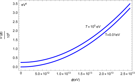
Figure 1: The effective potential (units in eV⁴) of the axion-neutrino thermal bath, for the model of Eq. (8), below $T_{D}\sim 1\,$MeV and down to $T\sim 0.01\,$eV, for two characteristic values of the temperature. No sign of a thermal phase transition exists for this simple interacting system.

As it can be seen in Fig. 1, no phase transition occurs. Indeed, the axion-neutrino effective potential has only one minimum at the origin, both at zero temperature and at high temperature. Thus in effect, the axion oscillations are not disturbed, even though the axion gets thermalized with the neutrino bath. This result is in contrast to Ref. [7], and now let us demonstrate the difference between our result and that of Ref. [7]. The problem between our approach and that of Ref. [7] is that in practise, the mass dependent logarithmic contributions between the zero temperature one-loop fermion and boson contributions are cancelled with the finite-temperature contributions, and specifically the cancellation occurs between the terms containing $\frac{m_{\phi}^{4}}{64\pi^{2}}\ln\left(m_{\phi}^{2}\right)$ for the boson part and $\frac{12m_{\nu}^{4}}{64\pi^{2}}\ln\left(m_{\nu}^{2}\right)$ for the neutrino contribution. In Ref. [7], this cancellation is not taken into account and thus it seems that the result is not valid, plus no other temperature dependent-mass containing terms are also not taken into account. We believe that our result is transparent, and no phase transition occurs at late-times for the thermalized axion-neutrino system. Let us note here that the era in which a possible phase transition is checked in the case at hand is in the temperature range $T\sim(0.1,0.01)\,$eV so basically in the redshift range $z\sim(385,37)$. Hence, if a phase transition occurs at late times, it has to occur when the temperature drops well below the neutrino decoupling temperature. The critical temperature should in principle be of the order of the neutrino mass, $m_{0}\sim 0.01$ so $T\sim 0.01$eV so it is expected that any possible phase transition will take place somewhere at the redshift interval $z\sim(385,37)$.

The absence of finite temperature phase transitions persists even if we consider a generalization of the above axion-neutrino system, considering $N$ different fermion flavors, with a $Z_{N}$ symmetric Lagrangian [7],

$$\mathcal{L}=\frac{1}{2}\partial_{\mu}\phi\partial^{\mu}\phi+\sum_{j=0}^{N-1}\left(i\bar{\nu}_{j}\gamma^{\mu}\partial_{\mu}\nu_{j}+\left(m_{0}+\epsilon^{i(\frac{\phi}{f}+\frac{2\pi j}{N})}\right)\bar{\nu}_{jL}\nu_{jR}\right)+\Lambda_{a}^{4}\left(1-\cos(\frac{\phi}{f})\right)\,.$$ (15)

The explicit chiral symmetry breaking terms generate quadratic divergences at one-loop level, so the effective Lagrangian further contains the following terms,

$$\sum_{j=0}^{N-1}\frac{m_{0}\epsilon\Lambda^{2}}{8\pi^{2}}\cos\left(\frac{\phi}{f}+\frac{2pj}{N}\right)\,.$$ (16)

the fermion masses in this case are,

$$M_{j}^{2}=m_{0}^{2}+\epsilon^{2}+2m_{0}\epsilon\cos\left(\frac{\phi}{f}+\frac{2pj}{N}\right)\,,$$ (17)

and due to the $Z_{N}$ symmetry we have the following relations that hold true,

$$\sum_{j=0}^{N-1}M_{j}^{2}=N(m_{0}^{2}+\epsilon^{2})\,,$$ (18)

$$\sum_{j=0}^{N-1}M_{j}^{4}=N\left(2m_{0}^{2}\epsilon^{2}+(m_{0}^{2}+\epsilon^{2})^{2}\right)\,.$$ (19)

In the $\bar{\mathrm{MS}}$ renormalization scheme, the one-loop finite temperature corrected axion-neutrino effective potential reads,

$$V(\phi) =\Lambda_{a}^{4}\left(1-\cos(\frac{\phi}{f})\right)+\frac{m_{\phi}^{4}}{64\pi^{2}}\left(\frac{a_{b}\,T^{2}}{\mu^{2}}-\frac{3}{2}\right)+\frac{m_{\phi}^{2}T^{2}}{24}-\frac{1}{12\pi}\left(m_{\phi}^{3/2}\right)T$$ (20)

$$-\sum_{j=0}^{N-1}\frac{3}{16}\frac{M_{j}^{4}}{\pi^{4}}\left(\log\left(\frac{M_{j}^{2}}{\mu^{2}}\right)-\frac{3}{2}\right)+\frac{3}{16\pi^{2}}\sum_{j=0}^{N-1}M_{j}^{4}\log\left(\frac{M_{j}^{2}}{a_{f}\,T^{2}}\right)+\sum_{j=0}^{N-1}M_{j}^{2}\frac{T^{2}}{4}\,,$$

where $\mu$ is the renormalization scale, and due to the fact that,

$$-\sum_{j=0}^{N-1}\frac{3}{16}\frac{M_{j}^{4}}{\pi^{4}}\left(\log\left(\frac{M_{j}^{2}}{\mu^{2}}\right)-\frac{3}{2}\right)+\frac{3}{16\pi^{2}}\sum_{j=0}^{N-1}M_{j}^{4}\log\left(\frac{M_{j}^{2}}{a_{f}\,T^{2}}\right)=$$ (21)

$$\sum_{j=0}^{N-1}\frac{3}{16}M_{j}^{4}\frac{3}{2}-\sum_{j=0}^{N-1}\frac{M_{j}^{4}}{\pi^{2}}\left(\log M_{j}^{2}-\log\mu^{2}\right)+\frac{3}{16\pi^{2}}\sum_{j=0}^{N-1}M_{j}^{4}\left(\log M_{j}^{4}-\log\left(a_{f}T^{2}\right)\right)\,,$$

the last two terms in the effective potential (20) can be written as follows,

$$-\sum_{j=0}^{N-1}\frac{3}{16}\frac{M_{j}^{4}}{\pi^{4}}\left(\log\left(\frac{a_{f}\,T^{2}}{\mu^{2}}\right)-\frac{3}{2}\right)+\sum_{j=0}^{N-1}M_{j}^{2}\frac{T^{2}}{4}\,.$$ (22)

Due to relations (18) and (19), the two terms above can be written as, (20),

$$-\sum_{j=0}^{N-1}\frac{3}{16}\frac{M_{j}^{4}}{\pi^{4}}\left(\log\left(\frac{a_{f}\,T^{2}}{\mu^{2}}\right)-\frac{3}{2}\right)=N\left(2m_{0}^{2}\epsilon^{2}+(m_{0}^{2}+\epsilon^{2})^{2}\right)\left(\log\left(\frac{a_{f}\,T^{2}}{\mu^{2}}\right)-\frac{3}{2}\right)\,,$$ (23)

and

$$\sum_{j=0}^{N-1}M_{j}^{2}\frac{T^{2}}{4}=\frac{N}{4}\left(m_{0}^{2}+\epsilon^{2}\right)T^{2}\,,$$ (24)

which are both field independent. This feature can also be seen by adding the relevant terms in Ref. [7], so basically the result of Ref. [7] cannot be correct, because in the fermion sector there is no field dependent term. Thus only the axion contributes to the $Z_{N}$ symmetric axion-neutrino system, and it can easily be shown that there is no phase transition regardless the value of the temperature, which is in contrast with the result of Ref. [7]. The discrepancy occurs due to the cancellation of the field dependent contributions in the effective potential, which we demonstrated above, which can also be observed in Ref. [7] but is not taken into account.

Now let us consider the axion and a single neutrino sector in the presence of a spontaneous breaking term of the chiral symmetry in the form $\sim\cos\left(\frac{\phi}{f}\right)$, in the absence of an explicit breaking term. The simple chiral symmetric axion-neutrino Lagrangian with a single neutrino species containing the cosine spontaneous chiral symmetry breaking potential for the axion scalar is,

$$\mathcal{L}=\frac{1}{2}\partial^{\mu}\phi\partial_{\mu}\phi+i\bar{\nu}_{L}\gamma^{\mu}\partial_{\mu}\nu_{L}+i\bar{\nu}_{R}\gamma^{\mu}\partial_{\mu}\nu_{R}+m_{0}\bar{\nu}_{L}\nu_{R}e^{i\frac{\phi}{f}}+\Lambda_{a}\left(1-\cos\left(\frac{\phi}{f}\right)\right)+\mathrm{H.C.}\,,$$ (25)

where in the same way as in the previous models, the term which couples the axion field with the neutrino may arise from a direct Yukawa coupling between the complex scalar field $\Phi$ associated with the spontaneous symmetry breaking of the primordial $U(1)$ Peccei-Quinn symmetry which gave rise to the axion. In the present case, the scale $\Lambda_{a}$ is basically connected with the energy scale at which the spontaneous breaking of the primordial $U(1)$ Peccei-Quinn symmetry breaking occurs. The cosine potential term of the axion breaks the chiral symmetry in the neutrino sector down to a residual $Z_{2}$ shift symmetry $\phi\to\phi+n\pi f$, which also protects the axion from having quadratic corrections in its mass from 1-loop contributions. Thus in the present case, the axion receives its mass by an undetermined non-perturbative mechanism and the residual $Z_{2}$ shift symmetry of the cosine potential protects the axion from receiving corrections to its mass due to one loop quadratic divergences. Such cosine potentials may arise in the theory in a non-perturbative way if the associated symmetry has an anomalous current. For the purposes of this letter, we shall assume that this cosine potential term does not arise from a fundamental theoretical process, but it is of unknown origin, or some non-perturbative arguments of the underlying theory give rise to this term. Also in the present context, one has not to take into account fifth forces in the neutrino sector, due to induced existence of the derivative couplings of the form $\sim\frac{1}{f}\partial^{\mu}\phi\bar{\nu}\gamma_{5}\gamma_{\mu}\nu$, because for small $\phi$ momentum, the $\phi$ emission and absorption amplitudes will tend to zero [7]. Due to this decoupling procedure, the axion $\phi$ will not be the mediator of a fifth force in the neutrino sector. However, as we showed in the previous models, in the presence of an explicit chiral symmetry breaking term accompanied with CP-violation, the Adler decoupling we discussed is violated, and thus fifth forces may arise in the neutrino sector, mediated by the axion. We can easily calculate the finite-temperature corrected effective potential for the axion-neutrino model, including the zero temperature one-loop corrections and the tree-order effective potential of the misalignment axion,

$$V(\phi)=V_{tree}+V^{1-loop}_{T=0}(\phi)+V^{1-loop}_{T\neq 0}(\phi)\,,$$ (26)

where for the tree potential,

$$V_{tree}=\frac{m_{a}^{2}}{2}\phi^{2}-\frac{\Lambda_{a}^{4}}{24f^{4}}\phi^{4}\,,$$ (27)

we again considered small displacements of the axion field from the minimum of the potential ($\frac{\phi}{f}\ll 1$), which are valid for the misalignment axion models. Also $m_{a}^{2}=\Lambda^{4}/f^{2}$ and with $V^{1-loop}_{T=0}(\phi)$ being equal to,

$$V^{1-loop}_{T=0}(\phi)=\frac{m_{\phi}^{4}}{64\pi^{2}}\left(\ln\frac{m_{\phi}^{2}}{\mu^{2}}-\frac{3}{2}\right)-\frac{3}{16}\frac{m_{0}^{4}}{\pi^{2}}\left(\ln\frac{m_{0}^{2}}{\mu^{2}}-\frac{3}{2}\right)\,,$$ (28)

with $\mu$ being again an arbitrary for the moment renormalization scale and $m_{\phi}^{2}=\frac{d^{2}V_{tree}}{d\phi^{2}}$. Also the one-loop finite-temperature correction term $V^{1-loop}_{T\neq 0}(\phi)$ reads,

$$V^{1-loop}_{T\neq 0}(\phi)=\frac{m_{0}T^{2}}{4}+\frac{3}{16\pi^{2}}m_{0}^{4}\ln\left(\frac{m_{0}^{2}}{a_{f}T^{2}}\right)+\frac{m_{\phi}^{2}T^{2}}{24}-\frac{1}{12\pi}m_{\phi}^{3}T-\frac{m_{\phi}^{4}}{64\pi^{2}}\ln\left(\frac{m_{\phi}^{2}}{a_{b}T^{2}}\right)\,,$$ (29)

and recall that $\ln(a_{b})=5.4076$ and $\ln(a_{f})=2.6351$. Notice again the cancellation between the mass-dependent one-loop terms at finite temperature and zero temperature for both the neutrino and the axion fields, therefore, the resulting effective potential reads,

$$V(\phi)=\frac{m_{a}^{2}}{2}\phi^{2}-\frac{\Lambda_{a}^{4}}{24f^{4}}\phi^{4}+\frac{m_{\phi}^{2}T^{2}}{24}-\frac{1}{12\pi}m_{\phi}^{3}T+\frac{m_{0}T^{2}}{4}+\frac{m_{\phi}^{4}}{64\pi^{2}}\left(\ln\left(\frac{a_{b}T^{2}}{\mu^{2}}\right)-\frac{3}{2}\right)-\frac{3m_{0}^{4}}{16\pi^{2}}\left(\ln\left(\frac{a_{f}T^{2}}{\mu^{2}}\right)-\frac{3}{2}\right)\,.$$ (30)

The same thermalization arguments for the neutrino-axion system hold true, as in the previous models thus the temperature above which the axion can be at thermal equilibrium with the axion background is beyond $T_{c}\sim 0.01\,$eV and below the neutrino electroweak decoupling temperature $T_{D}\sim 1\,$MeV, above which the neutrino is at thermal equilibrium with the particles which interact with it via the weak interactions.

Also in the context of the present model $\Lambda_{a}=\sqrt{m_{a}f}$. For the plots, we shall also assume that $\phi\ll f$, hence the effective mass of the axion at tree order is $m_{eff}^{2}=m_{a}^{2}-\frac{\phi^{2}}{24f^{4}}$. The effective potential at $T\sim 0.1\,$eV, $T\sim 10^{3}\,$eV and $T\sim 10^{5}\,$eV is plotted in Fig. 2.

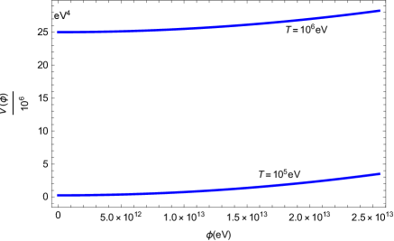
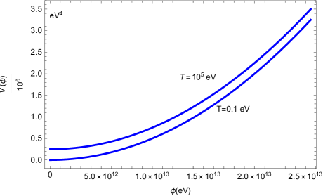
Figure 2: The effective potential (units in eV⁴) of the axion-neutrino thermal bath below $T_{D}\sim 1\,$MeV and up to $T\sim 0.1\,$eV, for three characteristic values of the temperature. No sign of a thermal phase transition exists for this simple interacting system.

As in the previous cases, it can be seen in Fig. 2, no phase transition occurs as the axion-neutrino effective potential has only one minimum at the origin, a situation which occurs both at zero temperature and at high temperature. Thus in effect, the axion oscillations are not disturbed in this case too, regardless the axion thermalization with the neutrino bath. The attribute of the first model we presented in this section, compared to the second model is that the first model respects the naturalness argument. Recall that by naturalness it is meant that, the mass scales of all particles participating in a Lagrangian must not be fined tuned, but instead must appear as a inherent to the theory consequence of some mechanism. As t’Hooft also claims, a parameter is considered naturally small if in its limit to zero, the symmetry structure of the Lagrangian is enhanced. In such a case the parameter will in general be multiplicatively renormalizable and can remain small at all orders in perturbation theory. Also, in a more restrictive way, in the strong naturalness case, the mass of ultralight particles must emerge on some symmetry breaking ground and not being fixed by hand. In the case at hand, the first model provides a mechanism for the generation of the axion mass, via an explicit chiral symmetry breaking term, so it is more complete from a phenomenological point of view, compared to the second model.

IV Late-time Phase Transitions Caused by the Higgs Portal Interactions of the Axion

Now let us consider an alternative scenario in which the Higgs portal affects the axion via higher order non-renormalizable operators. Such a scenario was recently considered in Ref. [50]. Specifically we shall assume that the axion is interacting with the Higgs particle via dimension six and dimension eight non-renormalizable operators. We assume that the Universe experiences the standard reheating era epoch and that the electroweak breaking occurs during the radiation domination era. Also we assume that the Universe reached a large reheating temperature, which is larger than $T\sim 100\,$GeV. When the temperature drops below $T\sim 100\,$GeV, the electroweak breaking occurs and thus the Higgs particle acquires a non-zero vacuum expectation value and via the Yukawa couplings and other interactions, gives mass to the Standard Model particles. With regard to the axion sector, without for the moment taking into account the neutrino sector, the axion potential has the form,

$$V_{a}(\phi)=m_{a}^{2}f_{a}^{2}\left(1-\cos\left(\frac{\phi}{f_{a}}\right)\right)\,,$$ (31)

which when $\phi/f_{a}<1$, can be approximated as,

$$V_{a}(\phi)\simeq\frac{1}{2}m_{a}^{2}\phi^{2}\,.$$ (32)

When considering the axion-neutrino sector, such a potential may arise in the way we described in the previous section, thus by a spontaneous symmetry breaking term of the chiral symmetry in the neutrino sector, or via an explicit breaking term of the chiral symmetry in the neutrino sector, which induces an axion mass via a one-loop quadratic divergence. Returning back to the Higgs-axion interaction, the dimension six and dimension eight non-renormalizable operators of the Higgs to the axion scalar are of the form [50] $\sim\lambda\frac{|H|^{2}\phi^{4}}{M^{2}}$ and $\sim g\frac{|H|^{2}\phi^{6}}{M^{4}}$, and thus the axion-Higgs effective potential at tree order is,

$$V(\phi,h)=V_{a}(\phi)-m_{H}^{2}|H|^{2}+\lambda_{H}|H|^{4}-\lambda\frac{|H|^{2}\phi^{4}}{M^{2}}+g\frac{|H|^{2}\phi^{6}}{M^{4}}\,,$$ (33)

with $V_{a}(\phi)$ appearing in Eq. (31). The Higgs scalar before the electroweak breaking has the form $H=\frac{h+ih_{1}}{\sqrt{2}}$ and the Higgs particle mass is $m_{H}=125$ GeV, while the Higgs self-coupling is defined through the relation $\frac{v}{\sqrt{2}}=\left(\frac{-m_{H}^{2}}{\lambda_{H}}\right)^{\frac{1}{2}}$, with $v$ being the electroweak symmetry breaking scale which is $v\simeq 246\,$GeV. The scale $M$ denotes the scale at which the effective field theory scale of the non-renormalizable dimension six and dimensions eight operators at which they originate from and are active. We shall assume that this effective scale $M$ is way higher than the electroweak breaking scale, and specifically we assume that $M$ is of the order $M=20-100\,$TeV. This choice is not accidental and is highly motivated by the fact that no particle has ever been observed at the LHC beyond the electroweak scale and up to energies of the order $\sim 15\,$TeV center-of-mass. Regarding the parameters $\lambda$ and $g$ these are the Wilson coefficients of the higher order effective field theory of the Higgs-axion sector, which will be assumed to be of the order $\lambda\sim\mathcal{O}(10^{-20})$ and $g\sim\mathcal{O}(10^{-5})$ for phenomenological reasons, see Ref. [50]. After the electroweak breaking, the standard thermal history in the Standard Model sector occurs, with a first order phase transition taking place. We shall mainly be interested in the axion sector and for temperatures below the neutrino decoupling sector. As we shall see, the presence of neutrinos accompanied with the higher order Higgs-axion interactions can cause a physically interesting situation, with a late-time phase transition occurring. The couplings of the Higgs to the axion do not affect the electroweak sector, the operators are non-renormalizable and thus the effects are significantly suppressed, but these operators can affect the late-time axion-neutrino system, causing a late-time phase transition during the post neutrino decoupling era. After the electroweak breaking, the Higgs particle obtains a vacuum expectation value, thus $H=v+\frac{h+ih_{1}}{\sqrt{2}}$, and therefore the higher dimensional operators are affected. Therefore, in the post electroweak breaking era, the axion effective potential $\mathcal{V}_{a}(\phi)$ becomes,

$$\mathcal{V}_{a}(\phi)=V_{a}(\phi)-\lambda\frac{v^{2}\phi^{4}}{M^{2}}+g\frac{v^{2}\phi^{6}}{M^{6}}\,,$$ (34)

where we defined $V_{a}(\phi)$ in Eq. (31). The behavior of the axion during the radiation domination era in this framework was studied in Ref. [50], but in this work we shall focus on the post neutrino decoupling era. Thus, let us write in a compact way the current theory, in which case the Lagrangian before the electroweak breaking is,

$$\mathcal{L}=\frac{1}{2}\partial^{\mu}H^{+}\partial_{\mu}H-m_{H}^{2}|H|^{2}+\lambda_{H}|H|^{4}-\lambda\frac{|H|^{2}\phi^{4}}{M^{2}}+g\frac{|H|^{2}\phi^{6}}{M^{4}}$$ (35)

$$+\frac{1}{2}\partial^{\mu}\phi\partial_{\mu}\phi+i\bar{\nu}_{L}\gamma^{\mu}\partial_{\mu}\nu_{L}+i\bar{\nu}_{R}\gamma^{\mu}\partial_{\mu}\nu_{R}+m_{0}\bar{\nu}_{L}\nu_{R}e^{i\frac{\phi}{f}}+\Lambda_{a}\left(1-\cos\left(\frac{\phi}{f}\right)\right)+\mathrm{H.C.}\,,$$

thus the tree order effective potential of the axion and neutrino system, during the post electroweak epoch is,

$$\mathcal{V}_{a}(\phi)=\frac{m_{a}^{2}}{2}\phi^{2}-\frac{\Lambda_{a}^{4}}{24f^{4}}\phi^{4}-\lambda\frac{v^{2}\phi^{4}}{M^{2}}+g\frac{v^{2}\phi^{6}}{M^{6}}\,,$$ (36)

and the tree order effective mass for the axion is $m_{eff}^{2}(\phi)$,

$$m_{eff}^{2}(\phi)=\frac{\partial^{2}V(\phi,h)}{\partial\phi^{2}}=m_{a}^{2}-\frac{6\lambda v^{2}\phi^{2}}{M^{2}}+\frac{15gv^{2}\phi^{4}}{M^{4}}\,,$$ (37)

which is derived from the second derivative of the tree order axion effective potential with respect to the axion field, that is $m_{eff}^{2}(\phi)=\frac{\partial^{2}\mathcal{V}_{a}(\phi)}{\partial\phi^{2}}$. Including the zero and finite temperature contributions to the effective potential for the axion-neutrino system, the final form of the effective potential is in the high temperature limit,

$$V_{a}^{1-loopT\neq 0}=\frac{m_{a}^{2}}{2}\phi^{2}-\frac{\Lambda_{a}^{4}}{24f^{4}}\phi^{4}-\lambda\frac{v^{2}\phi^{4}}{M^{2}}+g\frac{v^{2}\phi^{6}}{M^{6}}+\frac{m_{eff}^{2}(\phi)}{24}T^{2}$$ (38)

$$-\frac{T}{12\pi}\left(m_{eff}^{2}(\phi)\right)^{3/2}+\frac{m_{eff}^{4}(\phi)}{64\pi^{2}}\left(\ln a_{b}-\frac{3}{2}\right)++\frac{m_{eff}^{4}(\phi)}{64\pi^{2}}\ln\left(\frac{T^{2}}{\mu^{2}}\right)+\frac{m_{0}\,T^{2}}{4}-\frac{3\,m_{0}^{4}}{16\pi^{2}}\left(\ln\left(\frac{a_{f}T^{2}}{\mu^{2}}\right)-\frac{3}{2}\right)\,.$$

It can also be observed in this case that the logarithmic mass terms proportional to $m_{eff}^{4}(\phi)$ and $m_{0}^{4}$, both cancel in the $\bar{\mathrm{MS}}$ renormalization scheme, for both the fermion and boson sectors. The form of the potential in Eq. (38) is valid only in the high temperature limit, when $\frac{m_{eff}^{2}(\phi)}{T^{2}}\ll 1$ and $\frac{m_{0}}{T}\ll 1$. As we discussed thoroughly in the previous section, the axion and the neutrino can be considered at a coherent classical thermal equilibrium between ensembles of particles, beyond $T\sim m_{\nu}$. The thermal equilibrium between the axion and the neutrino continues until the temperature becomes of the order of the neutrino mass, at which point the neutrino decouples from the thermal equilibrium. Therefore, for the axion and the neutrino are considered to be at a coherent thermal equilibrium for $T\sim>0.01\,$eV, and the phase transition occurs approximately at $T\sim m_{0}\sim 0.01\,$eV, which we cannot approach in a perturbative way. In Fig. 3 we plot the behavior of the effective potential at high and low temperatures, in the temperature range $T\sim 10^{6}-0.01\,$eV, using three characteristic temperatures $T=10^{6}\,$eV, $T=10^{5}\,$eV and $T=0.1\,$eV. As it can be seen in Fig. 3, the potential at high temperature, which is very close to the era when the neutrino decouples from the electroweak thermal bath, has one minimum at the origin, and this picture continues to hold true until approximately $T\sim 10^{5}\,$eV where a second minimum is developed, with the two minima being separated by a potential barrier. The same physical picture continues to hold true until the temperature drops to $T=0.1\,$eV, however at $T\sim 10^{5}\,$eV the two minima are equally favorable energetically, but when the temperature drops to $T=0.1\,$eV, the second minimum away from the origin becomes more favorable energetically. This physical behavior points out to one thing only, a first order phase transition is likely to take place. The exciting thing is that this first order phase transition will take place at temperatures of the order $T\sim\mathcal{O}(0.1-0.01)$eV until the temperature becomes of the order of the neutrino mass, which we assumed to be of the order $m_{0}\sim 0.01\,$eV. This is a very interesting physical situation, since this first order phase transition is actually a late-time phase transition which happens globally to the Universe at the redshift corresponding to the phase transition temperature. Now the interesting part is the phase transition era’s redshift range, so if we assume that the temperature range at which the first order phase transition might take place is $T\sim 0.1-0.01\,$eV, the redshift range is $z\sim 385-37$, so it is possible to have a global, literally Universal, first order phase transition occurring in the era after the recombination, which occurred at $z\sim 1100$, at which era the CMB originates. It is vital to note that if the neutrino is absent from the model we presented in this section, the first order phase transition does not occur at all.

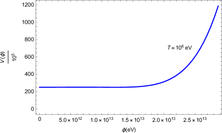
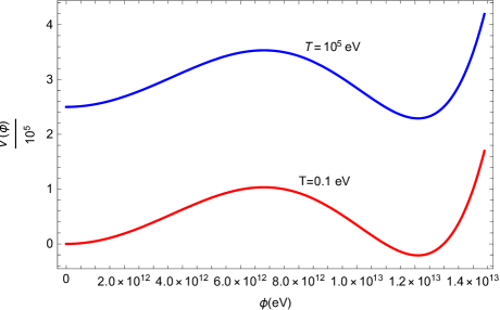
Figure 3: The effective potential (units in eV⁴) of the axion-neutrino thermal bath below $T_{D}\sim 1\,$MeV and down to $T\sim 0.01\,$eV, for three characteristic values of the temperature including the effects of a Higgs-axion coupling via higher order non-renormalizable operators. There is a clear indication of a first order phase transition in the system, which is controlled by the fermionic contribution.

This is a physically interesting situation from many aspects, and this scenario tights well with many astrophysical problems and potential issues, and also with the $H_{0}$-tension problems as we will discuss in the next section. In the model at hand, before the phase transition occurs, the axion is well protected at the origin of the effective potential, continuing its oscillations, not destabilized and thus it describes perfectly cold dark matter, however once the first order phase transition occurs, the axion is at the second minimum, which compared with the Higgs electroweak vacuum minimum is less energetically favorable, thus this minimum decays to the Higgs vacuum, as it was shown in [50]. The interesting part though is the phase transition itself, since such a physical picture destabilizes the whole dark matter of the Universe even instantaneously. Notice that this behavior occurs well beyond the neutrino decoupling from the electroweak sector, and until the temperature of the Universe is of the order of the neutrino mass. Also there is high possibility that this first order phase transition may give rise to gravitational radiation, which is rather unreachable to us via the interferometric gravitational wave experiments. Perhaps though it may have some observable effects on the CMB, but this needs further investigation, which we will not consider in this article though.

V A Qualitative Discussion on the Astrophysical and Cosmological Effects of a Late-time Phase Transition

In this section we shall qualitatively discuss the astrophysical and cosmological implications of a late-time first order phase transition in the Universe. As we shall see, these implications could be important for the post-CMB Universe and may play a crucial role on the generation of matter structure at high redshifts.

The early Universe is known to be very smooth and homogeneous, but it should have a mechanism that has generated small fluctuations in the total density of matter and radiation, which eventually grew into the large scale cosmological structure observed at present time. The $\Lambda$CDM model, is currently a benchmark model which predicts that the overall growth of the large scale structure should unavoidably be influenced by the properties of cold dark matter, which is currently thought to be the dominant form of matter in the Universe. In principle, the observations of the large scale structure of our Universe at high redshifts, which correspond to an age at which the Universe was quite younger, can certainly provide important information about the properties of dark matter at earlier times of our Universe. But these observations are rather challenging since they require precise measurements of distant and rather currently faint objects. Recent observations, for example the ones of the Dark Energy Survey and the Hyper Suprime-Cam survey [60], also provide constraints on the high redshift large scale structure. Overall, these observations indicate that the $\Lambda$CDM model is compatible with the data, but some discrepancies also exist that must explained. Specifically, the most persisting problem is the $\sigma_{8}$ issue having to do with the clustering at high redshifts with the large scale structure seeming more clustered than the predictions of the $\Lambda$CDM indicate. This indicates that the large scale the growth of structure which was formed after the CMB photons decoupled, was more efficient than the $\Lambda$CDM model predicts, thus unknown processes, like late-time phase transitions, may have taken place at the post-recombination era and these phase transitions may explain these discrepancies.

Furthermore, regarding the clustering issue, recent observations coming from the Lyman-alpha forest, which basically is a series of absorption lines observed in the spectrum of quasars which is caused by neutral hydrogen gas in the intergalactic medium, indicate that the clustering properties of these absorption lines can directly be used to probe the large scale structure of the Universe. Recent observations of the high redshift Lyman-alpha forest, indicate that the clustering of matter at high redshifts is stronger than the predictions of the $\Lambda$CDM model. Also the clustering of the temperature fluctuations of the CMB also indicates a larger clustering of matter, compared to the predictions of the $\Lambda$CDM model. The creation of large scale cosmological matter structure is very important, and we shall further discuss it, in the perspective of late-time first order phase transitions, which is exactly the type of phase transitions we presented in this paper. The observational data provided evidence for high redshift supermassive black holes [61, 62, 63, 64], and these redshifts correspond to an epoch in which the Universe was a billion years old. The explanation of the existence of such massive objects so far back in time is a challenge for the $\Lambda$CDM model accompanied with a standard inflationary scenario with Gaussian fluctuations. There exist works in the literature which discuss such challenges in a concrete way [65, 66, 67, 68, 69, 70, 71, 72, 73, 74]. Late-time phase transitions in the form of first order phase transitions can generate density fluctuations at relative high redshifts and thus can explain high redshift structure formation, without affecting significantly the large-angle CMB temperature anisotropies. Indeed, detailed studies already exist on this, which point out that late-time first order phase transitions can produce non-linear fluctuations that can generate massive structures of the order $M\sim 10^{6}-10^{10}\,M_{\odot}$, at redshifts $z\sim 10$ for a phase transition occurring at redshifts $z\sim 50-500$, see for example [16], which covers our scenario proposed in this paper which predicts phase transitions in the redshift range $z=[350,37]$. These density fluctuations which occur due to the first order phase transition, can be the source of anisotropies on the CMB polarization, and can be spotted in the integrated Sachs-Wolfe (ISW) effect. The CMB photons pass through these first order phase transition originating late-time density fluctuations, before these arrive to the detectors, and thus the overall effect is the sum of all the ISW contributions from all the distinct fluctuations. Also we need to mention the possibility of late-time stochastic gravitational waves caused by the bubble collisions of the first order phase transitions, however such a low frequency gravitational radiation cannot easily be verified experimentally. Several promising experiments related with the 21cm hydrogen line can in principle probe high redshift matter formation, up to a redshift of the order $z\sim 200$ [75, 76, 77, 78, 79, 80, 81]. These low-frequency radio array observations which are based on the redshift 21cm radiation, can be used to constrain late-time phase transition scenarios, matter formation and growth for redshifts up to $z\sim 200$. Late-time phase transitions might govern early matter formation, growth and clustering, and these physical scenarios can result to physically distinct situations compared to the $\Lambda$CDM model. It is notable, that apart from the fact that the late-time phase transitions can perhaps explain to some extent the high redshift matter formation and growth, it is also possible to provide evidence for the evolution and distribution of dwarf galaxies, which are at the core of $\Lambda$CDM’s shortcomings [16].

Late-time phase transitions are linked intrinsically with infrared physics. Phase transitions are likely to have occurred in the late-time Universe, at some point after the decoupling of the photons which form the cosmic microwave background (CMB) radiation. The reason is that the temperature anisotropy of the CMB, namely $\delta T/T$ would be affected if phase transitions occurred before the decoupling of the photons. The CMB last scattering surface is very smooth, thus if any phase transitions occurred prior to the decoupling, remnants of this transitions would disturb the CMB because the phase transitions lead to curvature perturbations which would have a direct effect on the CMB last scattering surface. In principle the density fluctuations at late times can be the source of structure formation at late times at the post decoupling of photons era, and at redshifts belonging in the forbidden region of the $\Lambda$CDM, at redshifts $z\geq 9$ and to mass scales of the order $M\sim 10^{18}M_{\odot}$ [11]. It is also possible that soft topological defects may be have been generated during the late-time phase transitions, which would have cause minimal effects on the CMB temperature anisotropy, thus the late-time phase transitions may be an alternative to the inflationary scenario, as a model that can explain the origin of structure in the Universe. Thus late-time phase transitions may generate large scale structure without conflict with the inflationary scenario. Indeed, such curvature fluctuations generated by late-time phase transitions may have secondary effects on the temperature anisotropy of the CMB, which will be generated by the propagation of the CMB photons through the late-time density fluctuations, causing a redshifting/blueshifting in the temperature anisotropy. One should also bare in mind that the late-time phase transitions may explain ionization and star formation at large redshifts $z\geq 30$, which could generate ionization. An interesting feature of late-time phase transitions is that they lead to large peculiar velocities at the time of the phase transition, due to large variations in density [11]. In addition, the cluster-cluster correlation may be explained by the fractal character generated from the late-time phase transitions [11].

It is finally worth to discuss the possible implications of a late-time phase transition on the $H_{0}$-tension. It is rather tempting to question the direct effects of the late-time phase transitions via the axion-neutrino couplings on the $H_{0}$-tension. In the context of the present paper, there exists the prediction of a fifth force among the neutrinos mediated by the axions. It is known [94] that strongly interacting 2-to-2 neutrino scatterings with an additional contribution to $\Delta N_{eff}$ is able to resolve the $H_{0}$-tension, see also [83]. Thus it would be interesting to examine such a perspective. Also, quite recently the effect the coupling of dark matter to neutrinos has been considered [84], in view of the Planck data, and the data hint towards a non-trivial interaction at 1$\sigma$. See also [85] for the impact of neutrinos on inflationary parameters. An additional motivation to investigate the implications of a late-time phase transition on the $H_{0}$-tension is the fact that such an abrupt physics change at late-times is known to affect the Cepheid variables [86, 87, 88], see also Refs. [89, 90] for similar scenarios. It is thus tempting to investigate the effects of late-time phase transitions on the $H_{0}$-tension from the abrupt physics change perspective. Another interesting perspective, potentially related with the $H_{0}$-tension, is how a late-time phase transition may change the expansion rate at the era of the phase transition, and thus change directly the calibration of observations related with the era of the phase transition. Finally, it is important to note that fifth forces, like the ones predicted in one of the models we presented, are also connected to the resolution of the $H_{0}$-tension [91, 92, 93] and also neutrinos are also connected to the $H_{0}$-tension [94, 95]. For a novel approach on probing fifth forces, see also [96] and also similar approaches for axion as mediators of the fifth force between neutrons, see [97, 98].

These questions should be answered in a focused and concrete way, but are out of the scopes of the present article. In the present section we only sketched on the possible late-time astrophysical effects of a late-time first order phase transition, without getting into actual details. Instead of this rather qualitative approach, detailed hydrodynamical calculations must be performed in order to see in a quantitative way the actual astrophysical implications of a late-time phase transitions on all the phenomena described qualitatively above. This task stretches far beyond the purposes of this article.

VI Conclusions

In this work we considered the possibility of a thermal late-time phase transition caused by some non-trivial axion-neutrino interaction which existed primordially. The axion-neutrino system is supposed to be coupled and the neutrino has a primordial chiral symmetry which is either broken spontaneously or explicitly. The two cases of broken chiral symmetry correspond to two distinct models of axion-neutrinos and we considered the phenomenological implications of both models. In the case of explicit chiral symmetry breaking, the axion receives its mass due to one-loop neutrino corrections and this model is compatible with the strong naturalness argument. In both cases, the axion is considered to be the misalignment axion from the primordial era up to the point at which the first order phase transition might take place, and below $T\sim m_{\nu}$, the neutrino decouples from the coherent/classical thermal interaction of neutrino and axion classical ensembles. Thus the axion acts a cold dark matter when no phase transition takes place, and it oscillates around the minimum of its cosine potential. As we demonstrated, there is no phase transition in the axion-neutrino system, since its effective potential is not destabilized from the origin due to thermal corrections, contrary to the existing literature. However, if the axion interacts with the Higgs particle via higher order non-renormalizable operators, the axion-neutrino effective potential is destabilized and a second energetically more favorable minimum is developed. Thus a first order phase transition occurs caused by the axion-neutrino interaction, in which as it seems, the neutrino plays an important role. Thus in this scenario, the axion acted as cold dark matter from the primordial era of the Universe, down to the point that the temperature of the Universe is $T\sim 1\,$MeV, at which point, the axion is destabilized and a first order phase transition occurs somewhere in the temperature range $T\sim 0.1-0.01\,$eV, and the axion vacuum penetrates to the more energetically favorable vacuum. However, the Higgs vacuum is more energetically favorable than the axion, and thus the axion minimum decays instantly to the Higgs vacuum. The late-time phase transition occurs at the redshift range $z\sim 385-37$, thus it is a post-CMB phase transition, with no effect on the temperature anisotropy of the CMB. However, such late-time phase transitions affect the density fluctuations, which can be sources for late-time structure formation. Thus high redshift large scale structure and clustering beyond $z\geq 9$ may be explained by such late-time phase transitions. It is challenging for astronomers to find hints of large scale structure at high redshifts and the James Webb Space Telescope might help towards this perspective. We explored in detail, in a qualitative way, the phenomenological implications of late-time first order phase transitions in the axion-neutrino sector both at the astrophysical and cosmological level. What now remains is to quantitatively address the issues discussed here qualitatively, at both cosmological and astrophysical level. This paper’s aim was to point out that the physics of the far infrared might have more to offer than meets the eye.

References

- [1] S. Nojiri, S. D. Odintsov and V. K. Oikonomou, Phys. Rept. 692 (2017) 1 [arXiv:1705.11098 [gr-qc]].
-
[2]
S. Capozziello, M. De Laurentis,
Phys. Rept. 509, 167 (2011);
V. Faraoni and S. Capozziello, Fundam. Theor. Phys. 170 (2010). - [3] S. Nojiri, S.D. Odintsov, eConf C0602061, 06 (2006) [Int. J. Geom. Meth. Mod. Phys. 4, 115 (2007)].
- [4] S. Nojiri, S.D. Odintsov, Phys. Rept. 505, 59 (2011);
- [5] G. J. Olmo, Int. J. Mod. Phys. D 20 (2011) 413 [arXiv:1101.3864 [gr-qc]].
- [6] E. W. Kolb and Y. Wang, Phys. Rev. D 45 (1992), 4421-4427 doi:10.1103/PhysRevD.45.4421
- [7] J. A. Frieman, C. T. Hill and R. Watkins, Phys. Rev. D 46 (1992), 1226-1238 doi:10.1103/PhysRevD.46.1226
- [8] G. M. Fuller and D. N. Schramm, Phys. Rev. D 45 (1992), 2595-2600 doi:10.1103/PhysRevD.45.2595
- [9] J. R. Primack and M. A. Sher, Nature 288 (1980), 680-681 doi:10.1038/288680a0
- [10] I. Wasserman, Phys. Rev. Lett. 57 (1986), 2234-2236 doi:10.1103/PhysRevLett.57.2234
- [11] C. T. Hill, D. N. Schramm and J. N. Fry, Comments Nucl. Part. Phys. 19 (1989) no.1, 25-39 FERMILAB-PUB-88-120-A.
- [12] W. H. Press, B. S. Ryden and D. N. Spergel, Phys. Rev. Lett. 64 (1990), 1084 doi:10.1103/PhysRevLett.64.1084
- [13] X. c. Luo and D. N. Schramm, Astrophys. J. 421 (1994), 393-399 doi:10.1086/173658
- [14] S. Dutta, S. D. H. Hsu, D. Reeb and R. J. Scherrer, Phys. Rev. D 79 (2009), 103504 doi:10.1103/PhysRevD.79.103504 [arXiv:0902.4699 [astro-ph.CO]].
- [15] N. Ramberg, W. Ratzinger and P. Schwaller, JCAP 02 (2023), 039 doi:10.1088/1475-7516/2023/02/039 [arXiv:2209.14313 [hep-ph]].
- [16] A. V. Patwardhan and G. M. Fuller, Phys. Rev. D 90 (2014) no.6, 063009 doi:10.1103/PhysRevD.90.063009 [arXiv:1401.1923 [astro-ph.CO]].
- [17] J. Preskill, M. B. Wise and F. Wilczek, Phys. Lett. 120B (1983) 127. doi:10.1016/0370-2693(83)90637-8
- [18] L. F. Abbott and P. Sikivie, Phys. Lett. 120B (1983) 133. doi:10.1016/0370-2693(83)90638-X
- [19] M. Dine and W. Fischler, Phys. Lett. 120B (1983) 137. doi:10.1016/0370-2693(83)90639-1
- [20] D. J. E. Marsh, Phys. Rept. 643 (2016) 1 [arXiv:1510.07633 [astro-ph.CO]].
- [21] P. Sikivie, Lect. Notes Phys. 741 (2008) 19 [astro-ph/0610440].
- [22] G. G. Raffelt, Lect. Notes Phys. 741 (2008) 51 [hep-ph/0611350].
- [23] A. D. Linde, Phys. Lett. B 259 (1991) 38.
- [24] R. T. Co, L. J. Hall and K. Harigaya, Phys. Rev. Lett. 124 (2020) no.25, 251802 doi:10.1103/PhysRevLett.124.251802 [arXiv:1910.14152 [hep-ph]].
- [25] R. T. Co, L. J. Hall, K. Harigaya, K. A. Olive and S. Verner, JCAP 08 (2020), 036 doi:10.1088/1475-7516/2020/08/036 [arXiv:2004.00629 [hep-ph]].
- [26] B. Barman, N. Bernal, N. Ramberg and L. Visinelli, [arXiv:2111.03677 [hep-ph]].
- [27] M. C. D. Marsh, H. R. Russell, A. C. Fabian, B. P. McNamara, P. Nulsen and C. S. Reynolds, JCAP 1712 (2017) no.12, 036 [arXiv:1703.07354 [hep-ph]].
- [28] S. D. Odintsov and V. K. Oikonomou, Phys. Rev. D 99 (2019) no.6, 064049 [arXiv:1901.05363 [gr-qc]].
- [29] S. D. Odintsov and V. K. Oikonomou, Phys. Rev. D 99 (2019) no.10, 104070 [arXiv:1905.03496 [gr-qc]].
- [30] A.S.Sakharov and M.Yu.Khlopov, Yadernaya Fizika (1994) V. 57, PP. 514- 516. ( Phys.Atom.Nucl. (1994) V. 57, PP. 485-487)
- [31] V. Anastassopoulos et al. [CAST Collaboration], Nature Phys. 13 (2017) 584 [arXiv:1705.02290 [hep-ex]].
- [32] P. Sikivie, Phys. Rev. Lett. 113 (2014) no.20, 201301 [arXiv:1409.2806 [hep-ph]].
- [33] P. Sikivie, Phys. Lett. B 695 (2011) 22 [arXiv:1003.2426 [astro-ph.GA]].
- [34] P. Sikivie and Q. Yang, Phys. Rev. Lett. 103 (2009) 111301 [arXiv:0901.1106 [hep-ph]].
- [35] E. Masaki, A. Aoki and J. Soda, arXiv:1909.11470 [hep-ph].
- [36] J. Soda and D. Yoshida, Galaxies 5 (2017) no.4, 96.
- [37] J. Soda and Y. Urakawa, Eur. Phys. J. C 78 (2018) no.9, 779 [arXiv:1710.00305 [astro-ph.CO]].
- [38] A. Aoki and J. Soda, Phys. Rev. D 96 (2017) no.2, 023534 [arXiv:1703.03589 [astro-ph.CO]].
- [39] A. Arvanitaki, S. Dimopoulos, M. Galanis, L. Lehner, J. O. Thompson and K. Van Tilburg, arXiv:1909.11665 [astro-ph.CO].
- [40] A. Arvanitaki, M. Baryakhtar, S. Dimopoulos, S. Dubovsky and R. Lasenby, Phys. Rev. D 95 (2017) no.4, 043001 [arXiv:1604.03958 [hep-ph]].
- [41] C. S. Machado, W. Ratzinger, P. Schwaller and B. A. Stefanek, arXiv:1912.01007 [hep-ph].
- [42] T. Tenkanen and L. Visinelli, JCAP 1908 (2019) 033 [arXiv:1906.11837 [astro-ph.CO]].
- [43] G. Y. Huang and S. Zhou, Phys. Rev. D 100 (2019) no.3, 035010 [arXiv:1905.00367 [hep-ph]].
- [44] D. Croon, R. Houtz and V. Sanz, JHEP 1907 (2019) 146 [arXiv:1904.10967 [hep-ph]].
- [45] F. V. Day and J. I. McDonald, JCAP 1910 (2019) no.10, 051 [arXiv:1904.08341 [hep-ph]].
- [46] V. K. Oikonomou, EPL 139 (2022) no.6, 69004 doi:10.1209/0295-5075/ac8fb2 [arXiv:2209.08339 [hep-ph]].
- [47] V. K. Oikonomou, Phys. Rev. D 106 (2022) no.4, 044041 doi:10.1103/PhysRevD.106.044041 [arXiv:2208.05544 [gr-qc]].
- [48] S. D. Odintsov and V. K. Oikonomou, EPL 129 (2020) no.4, 40001 doi:10.1209/0295-5075/129/40001 [arXiv:2003.06671 [gr-qc]].
- [49] V. K. Oikonomou, Phys. Rev. D 103 (2021) no.4, 044036 doi:10.1103/PhysRevD.103.044036 [arXiv:2012.00586 [astro-ph.CO]].
- [50] V. K. Oikonomou, Phys. Rev. D 107 (2023) no.6, 064071 doi:10.1103/PhysRevD.107.064071 [arXiv:2303.05889 [hep-ph]].
- [51] L. Di Luzio, M. Giannotti, E. Nardi and L. Visinelli, Phys. Rept. 870 (2020), 1-117 doi:10.1016/j.physrep.2020.06.002 [arXiv:2003.01100 [hep-ph]].
- [52] L. Visinelli and S. Vagnozzi, Phys. Rev. D 99 (2019) no.6, 063517 doi:10.1103/PhysRevD.99.063517 [arXiv:1809.06382 [hep-ph]].
- [53] K. Mazde and L. Visinelli, JCAP 01 (2023), 021 doi:10.1088/1475-7516/2023/01/021 [arXiv:2209.14307 [astro-ph.CO]].
- [54] G. Lambiase, L. Mastrototaro and L. Visinelli, JCAP 01 (2023), 011 doi:10.1088/1475-7516/2023/01/011 [arXiv:2207.08067 [hep-ph]].
- [55] N. Ramberg and L. Visinelli, Phys. Rev. D 99 (2019) no.12, 123513 doi:10.1103/PhysRevD.99.123513 [arXiv:1904.05707 [astro-ph.CO]].
- [56] C. T. Hill and G. G. Ross, Nucl. Phys. B 311 (1988), 253-297 doi:10.1016/0550-3213(88)90062-4
- [57] N. Aghanim et al. [Planck], Astron. Astrophys. 641 (2020), A6 [erratum: Astron. Astrophys. 652 (2021), C4] doi:10.1051/0004-6361/201833910 [arXiv:1807.06209 [astro-ph.CO]].
- [58] S. Hoof and L. Schulz, JCAP 03 (2023), 054 doi:10.1088/1475-7516/2023/03/054 [arXiv:2212.09764 [hep-ph]].
- [59] H. J. Li and W. Chao, Phys. Rev. D 107 (2023) no.6, 063031 doi:10.1103/PhysRevD.107.063031 [arXiv:2211.00524 [hep-ph]].
- [60] T. M. C. Abbott et al. [DES], Phys. Rev. D 99 (2019) no.12, 123505 doi:10.1103/PhysRevD.99.123505 [arXiv:1810.02499 [astro-ph.CO]].
- [61] X. Fan et al. [SDSS], Astron. J. 122 (2001), 2833 doi:10.1086/324111 [arXiv:astro-ph/0108063 [astro-ph]].
- [62] X. Fan et al. [SDSS], Astron. J. 125 (2003), 1649 doi:10.1086/368246 [arXiv:astro-ph/0301135 [astro-ph]].
- [63] C. J. Willott, R. J. McLure and M. J. Jarvis, Astrophys. J. Lett. 587 (2003), L15-L18 doi:10.1086/375126 [arXiv:astro-ph/0303062 [astro-ph]].
- [64] D. J. Mortlock, S. J. Warren, B. P. Venemans, M. Patel, P. C. Hewett, R. G. McMahon, C. Simpson, T. Theuns, E. A. Gonzales-Solares and A. Adamson, et al. Nature 474 (2011), 616 doi:10.1038/nature10159 [arXiv:1106.6088 [astro-ph.CO]].
- [65] Z. Haiman and A. Loeb, Astrophys. J. 552 (2001), 459 doi:10.1086/320586 [arXiv:astro-ph/0011529 [astro-ph]].
- [66] J. Yoo and J. Miralda-Escude, Astrophys. J. Lett. 614 (2004), L25-L28 doi:10.1086/425416 [arXiv:astro-ph/0406217 [astro-ph]].
- [67] S. L. Shapiro, Astrophys. J. 620 (2005), 59-68 doi:10.1086/427065 [arXiv:astro-ph/0411156 [astro-ph]].
- [68] M. Y. Khlopov, S. G. Rubin and A. S. Sakharov, Astropart. Phys. 23 (2005), 265 doi:10.1016/j.astropartphys.2004.12.002 [arXiv:astro-ph/0401532 [astro-ph]].
- [69] M. Volonteri and M. J. Rees, Astrophys. J. 633 (2005), 624-629 doi:10.1086/466521 [arXiv:astro-ph/0506040 [astro-ph]].
- [70] M. Volonteri and M. J. Rees, Astrophys. J. 650 (2006), 669-678 doi:10.1086/507444 [arXiv:astro-ph/0607093 [astro-ph]].
- [71] A. R. King and J. E. Pringle, Mon. Not. Roy. Astron. Soc. 373 (2006), L93-L97 doi:10.1111/j.1745-3933.2006.00249.x [arXiv:astro-ph/0609598 [astro-ph]].
- [72] Y. X. Li, L. Hernquist, B. Robertson, T. J. Cox, P. F. Hopkins, V. Springel, L. Gao, T. Di Matteo, A. R. Zentner and A. Jenkins, et al. Astrophys. J. 665 (2007), 187-208 doi:10.1086/519297 [arXiv:astro-ph/0608190 [astro-ph]].
- [73] N. Kawakatu and K. Wada, Astrophys. J. 706 (2009), 676-686 doi:10.1088/0004-637X/706/1/676 [arXiv:0910.1379 [astro-ph.CO]].
- [74] D. Sijacki, V. Springel and M. G. Haehnelt, Mon. Not. Roy. Astron. Soc. 400 (2009), 100 doi:10.1111/j.1365-2966.2009.15452.x [arXiv:0905.1689 [astro-ph.CO]].
- [75] A. Loeb and M. Zaldarriaga, Phys. Rev. Lett. 92 (2004), 211301 doi:10.1103/PhysRevLett.92.211301 [arXiv:astro-ph/0312134 [astro-ph]].
- [76] S. Furlanetto, S. P. Oh and F. Briggs, Phys. Rept. 433 (2006), 181-301 doi:10.1016/j.physrep.2006.08.002 [arXiv:astro-ph/0608032 [astro-ph]].
- [77] M. F. Morales and J. S. B. Wyithe, Ann. Rev. Astron. Astrophys. 48 (2010), 127-171 doi:10.1146/annurev-astro-081309-130936 [arXiv:0910.3010 [astro-ph.CO]].
- [78] J. C. Pober, A. Liu, J. S. Dillon, J. E. Aguirre, J. D. Bowman, R. F. Bradley, C. L. Carilli, D. R. DeBoer, J. N. Hewitt and D. C. Jacobs, et al. Astrophys. J. 782 (2014), 66 doi:10.1088/0004-637X/782/2/66 [arXiv:1310.7031 [astro-ph.CO]].
- [79] M. Zaldarriaga, S. R. Furlanetto and L. Hernquist, Astrophys. J. 608 (2004), 622-635 doi:10.1086/386327 [arXiv:astro-ph/0311514 [astro-ph]].
- [80] M. F. Morales, B. Hazelton, I. Sullivan and A. Beardsley, Astrophys. J. 752 (2012), 137 doi:10.1088/0004-637X/752/2/137 [arXiv:1202.3830 [astro-ph.IM]].
- [81] J. R. Pritchard and A. Loeb, Rept. Prog. Phys. 75 (2012), 086901 doi:10.1088/0034-4885/75/8/086901 [arXiv:1109.6012 [astro-ph.CO]].
- [82] C. D. Kreisch, F. Y. Cyr-Racine and O. Doré, Phys. Rev. D 101 (2020) no.12, 123505 doi:10.1103/PhysRevD.101.123505 [arXiv:1902.00534 [astro-ph.CO]].
- [83] M. Park, C. D. Kreisch, J. Dunkley, B. Hadzhiyska and F. Y. Cyr-Racine, Phys. Rev. D 100 (2019) no.6, 063524 doi:10.1103/PhysRevD.100.063524 [arXiv:1904.02625 [astro-ph.CO]].
- [84] P. Brax, C. van de Bruck, E. Di Valentino, W. Giarè and S. Trojanowski, [arXiv:2305.01383 [astro-ph.CO]].
- [85] M. Gerbino, K. Freese, S. Vagnozzi, M. Lattanzi, O. Mena, E. Giusarma and S. Ho, Phys. Rev. D 95 (2017) no.4, 043512 doi:10.1103/PhysRevD.95.043512 [arXiv:1610.08830 [astro-ph.CO]].
- [86] L. Perivolaropoulos and F. Skara, New Astron. Rev. 95 (2022), 101659 doi:10.1016/j.newar.2022.101659 [arXiv:2105.05208 [astro-ph.CO]].
- [87] L. Perivolaropoulos and F. Skara, Phys. Rev. D 104 (2021) no.12, 123511 doi:10.1103/PhysRevD.104.123511 [arXiv:2109.04406 [astro-ph.CO]].
- [88] L. Perivolaropoulos, Universe 8 (2022) no.5, 263 doi:10.3390/universe8050263 [arXiv:2201.08997 [astro-ph.EP]].
- [89] S. D. Odintsov and V. K. Oikonomou, EPL 137 (2022) no.3, 39001 doi:10.1209/0295-5075/ac52dc [arXiv:2201.07647 [gr-qc]].
- [90] S. D. Odintsov and V. K. Oikonomou, EPL 139 (2022) no.5, 59003 doi:10.1209/0295-5075/ac8a13 [arXiv:2208.07972 [gr-qc]].
- [91] H. Desmond and J. Sakstein, Phys. Rev. D 102 (2020) no.2, 023007 doi:10.1103/PhysRevD.102.023007 [arXiv:2003.12876 [astro-ph.CO]].
- [92] J. Sakstein, H. Desmond and B. Jain, Phys. Rev. D 100 (2019) no.10, 104035 doi:10.1103/PhysRevD.100.104035 [arXiv:1907.03775 [astro-ph.CO]].
- [93] H. Desmond, B. Jain and J. Sakstein, Phys. Rev. D 100 (2019) no.4, 043537 [erratum: Phys. Rev. D 101 (2020) no.6, 069904; erratum: Phys. Rev. D 101 (2020) no.12, 129901] doi:10.1103/PhysRevD.100.043537 [arXiv:1907.03778 [astro-ph.CO]].
- [94] C. D. Kreisch, F. Y. Cyr-Racine and O. Doré, Phys. Rev. D 101 (2020) no.12, 123505 doi:10.1103/PhysRevD.101.123505 [arXiv:1902.00534 [astro-ph.CO]].
- [95] J. Venzor, G. Garcia-Arroyo, A. Pérez-Lorenzana and J. De-Santiago, [arXiv:2303.12792 [astro-ph.CO]].
- [96] Y. D. Tsai, Y. Wu, S. Vagnozzi and L. Visinelli, JCAP 04 (2023), 031 doi:10.1088/1475-7516/2023/04/031 [arXiv:2107.04038 [hep-ph]].
- [97] A. Capolupo, S. M. Giampaolo and A. Quaranta, Eur. Phys. J. C 81 (2021) no.12, 1116 doi:10.1140/epjc/s10052-021-09888-x [arXiv:2102.13206 [hep-ph]].
- [98] A. Capolupo, S. M. Giampaolo and A. Quaranta, [arXiv:2305.07536 [hep-ph]].