MBIR Training for a 2.5D DL network in X-ray CT

Abstract In computed tomographic imaging, model based iterative reconstruction methods have generally shown better image quality than the more traditional, faster filtered backprojection technique. The cost we have to pay is that MBIR is computationally expensive. In this work we train a 2.5D deep learning (DL) network to mimic MBIR quality image. The network is realized by a modified Unet, and trained using clinical FBP and MBIR image pairs. We achieve the quality of MBIR images faster and with a much smaller computation cost. Visually and in terms of noise power spectrum (NPS), DL-MBIR images have texture similar to that of MBIR, with reduced noise power. Image profile plots, NPS plots, standard deviation, etc. suggest that the DL-MBIR images result from a successful emulation of an MBIR operator.

1 Introduction

X-ray computed tomography has become a important tool in applications such as healthcare diagnostics, security inspection, and non-destructive testing. The industry preferred method of reconstruction is filtered backprojection (FBP) and its popularity is owed to its speed and low computational cost. Iterative methods such as model-based iterative reconstruction (MBIR) generally have better image quality than FBP and do better in limiting image artifacts [1, 2].

MBIR is a computationally expensive and potentially slow reconstruction method since it entails repeated forward projection of the estimated image and back projection of the sinogram residual error. Even with fast GPUs becoming the norm, MBIR may take minutes compared to an FBP reconstruction that can be performed in seconds. The computational cost and reconstruction time have been deterents in wide adoption of MBIR.

In recent years, deep learning has made serious inroads in CT applications. It is applied in sinogram and image domains and sometimes in both. It has been applied in low signal correction [3], image denoising [4, 5], and metal artifact reduction [6].

Ziabari, et al [7] showed that a 2.5D deep neural network, with proper training, can effectively learn a mapping from an FBP image to MBIR. In this paper we expand on their work and study the characteristics of output from networks trained to simulate MBIR with a highly efficient neural network implementation.

2 Methods

We will first train a deep neural network, which we will, similarly to [7], entitle DL-MBIR. Our aim is to train the network to closely approximate MBIR images from FBP images. The training input is FBP images and the target is MBIR images from the same data. Let $X_{FBP}$ be the input to the network, $X_{MBIR}$ be the target, and $\sigma$ represents a hypothetical mapping such that $\sigma:X_{MBIR}\rightarrow X_{FBP}$. Let $f_{DL\text{-}MBIR_{Z}}$ be the DL neural network with $Z$ number of input channels. During the training phase:

$$\hat{f}_{DL\text{-}MBIR_{Z}}=\operatorname*{argmin}_{f_{DL\text{-}MBIR_{Z}}}{\big{|}}{\big{|}}f_{DL\text{-}MBIR_{Z}}(X_{FBP})-X_{MBIR}{\big{|}}{\big{|}}_{2}$$ (1)

$f_{DL\text{-}MBIR_{Z}}$ can be thought of as the inverse of $\sigma$, i.e. $f_{DL\text{-}MBIR_{Z}}=\sigma^{-1}$. During the training phase, the weights of $f_{DL\text{-}MBIR_{Z}}$ are randomly initialized and then adjusted in several iterations using error backpropagation. Once the number of iterations is exhausted or the convergence criteria is met, the training stops.

For training, 4 pairs of clinical exams were selected. Each pair had one FBP image volume and the corresponding MBIR volume. Each image volume had about 200 slices, resulting in about 800 training image pairs. A modified version of Unet [8] was chosen as the network architecture. The learning rate was set to $0.0001$ and 2 GPUs were used. Training and inferencing were done on Tensorflow/Keras. Training was run for 300 epochs. 3 versions of DL-MBIR were trained: $DL\text{-}MBIR_{1}$ was trained with inputs with 1 channel i.e. 1 axial slice, $DL\text{-}MBIR_{3}$ was trained with 3-channel inputs and $DL\text{-}MBIR_{5}$ was trained with 5-channel inputs. Having adjacent slices in the input provides additional information to the DL network [7] and helps train it better. Figure 1 shows the DL architecture and the training setup.

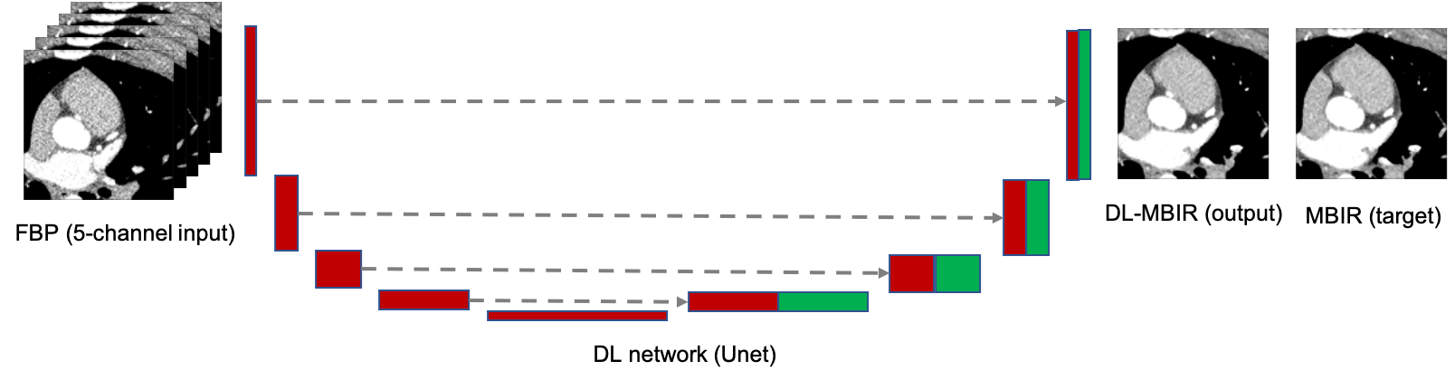
Figure 1: DL architecture and training setup. This is a modified form of Unet. Layers on the left denote the contracting path where features are compressed from image towards latent space but the number of features increases. Layers on the right denote the expanding path where feature are decompressed from latent space towards corrected image but the number of features decreases.

3 Results

A cardiac FBP image was inferenced on the trained DL-MBIR network. Inference time for every network was between 4 and 6 seconds, and it goes up with the increase in the number of input channels. The MBIR version of the same exam was also available. Figure 3 shows a comparison, for 4 slices – LABEL:sub@fig:Image_10, LABEL:sub@fig:Image_50, LABEL:sub@fig:Image_90, and LABEL:sub@fig:Image_170 in the image volume, among MBIR image, FBP image, and the outputs of $DL\text{-}MBIR_{Z}$, where $Z=1,\ 3,\ 5$. Figure 4 shows a comparison, for the same slices in the image volume, among difference between images and the MBIR images. Figure 5 has a profile plot to show the comparison of $DL\text{-}MBIR_{Z}$ and FBP images w.r.t the MBIR images.

Peak signal to noise ratio (PSNR) is another measure of similarity between images and is closely related to mean squared error. A higher value would mean that the image is closer to the reference image. Figure 2 is a plot of PSNR of all slices within the images with MBIR as the reference image. Table 1 has some other metrics of comparison among the images, such as averaged (across slices) PSNR, standard deviation (std) within regions of interest (RoIs), and average CT number within those RoIs.

The noise power spectrum (NPS) is a reliable tool for demonstrating similarity in the image texture. To measure NPS, uniform region patches from one of the cardiac chambers were extracted from each image. Then NPS was measured for all patches and averaged. Then 1D radial profile was measured from the 2D NPS. Figure 6 shows NPS in the uniform region within one of the cardiac chambers.

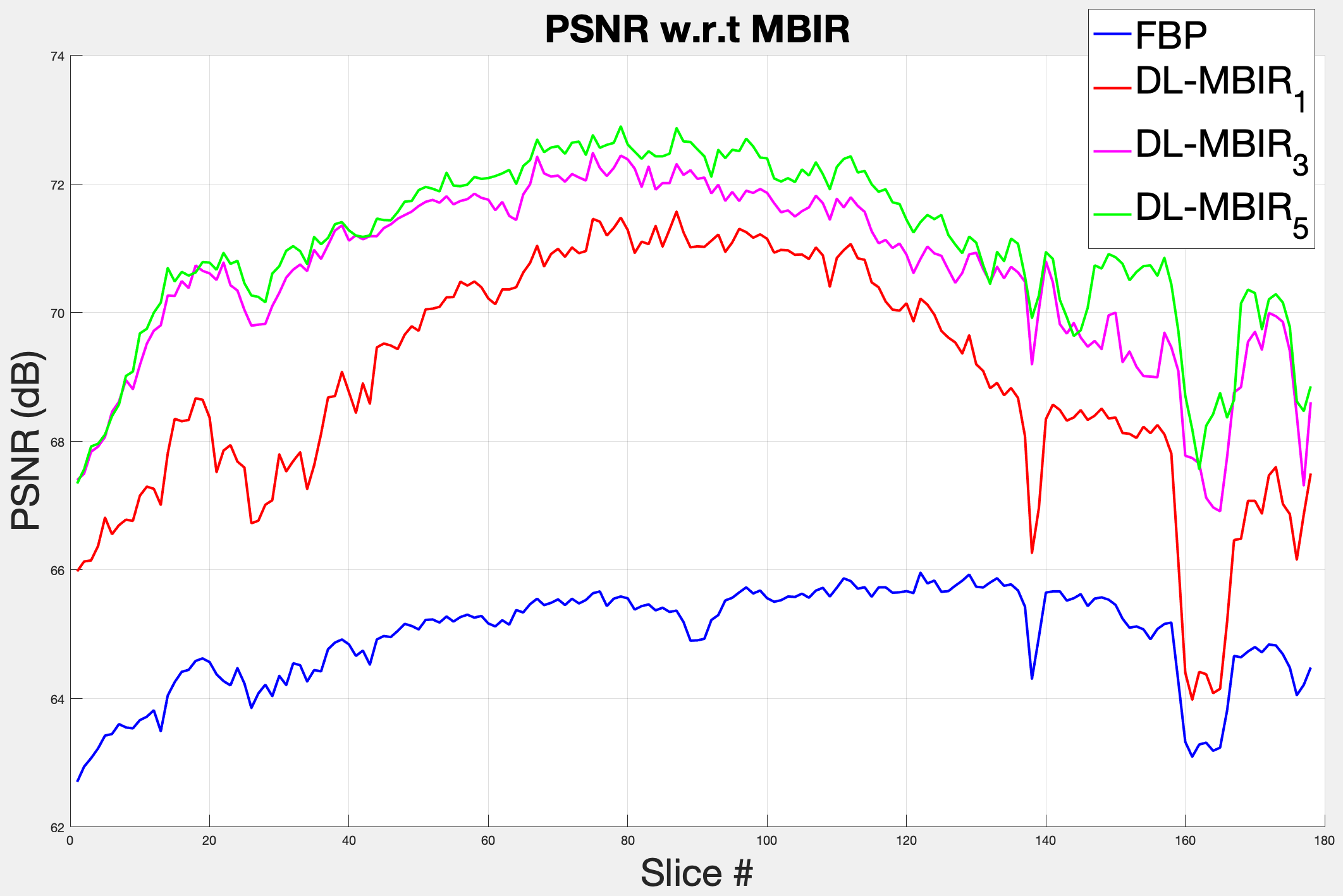
Figure 2: PSNR (with MBIR image as reference). PSNR values are in dB. X axis represents the axial slices in the image volume.

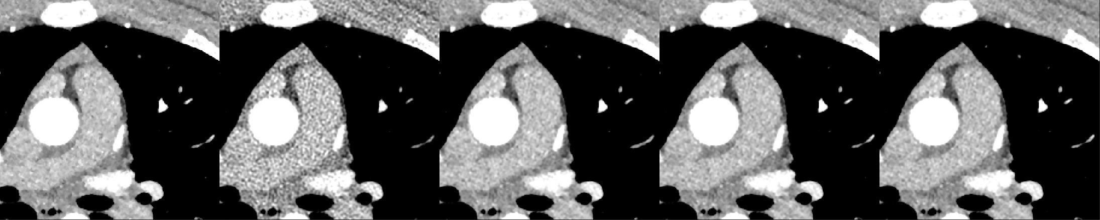
(a)

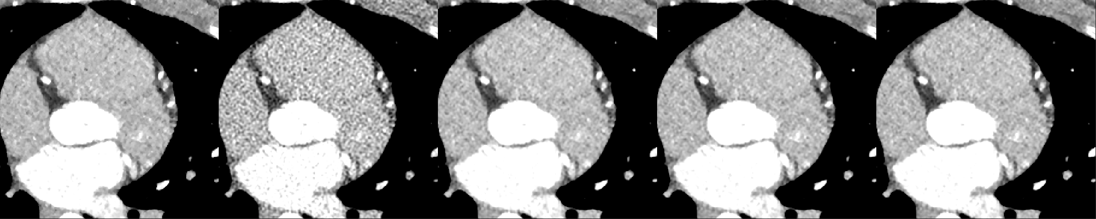
(b)

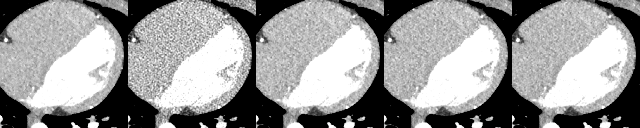
(c)

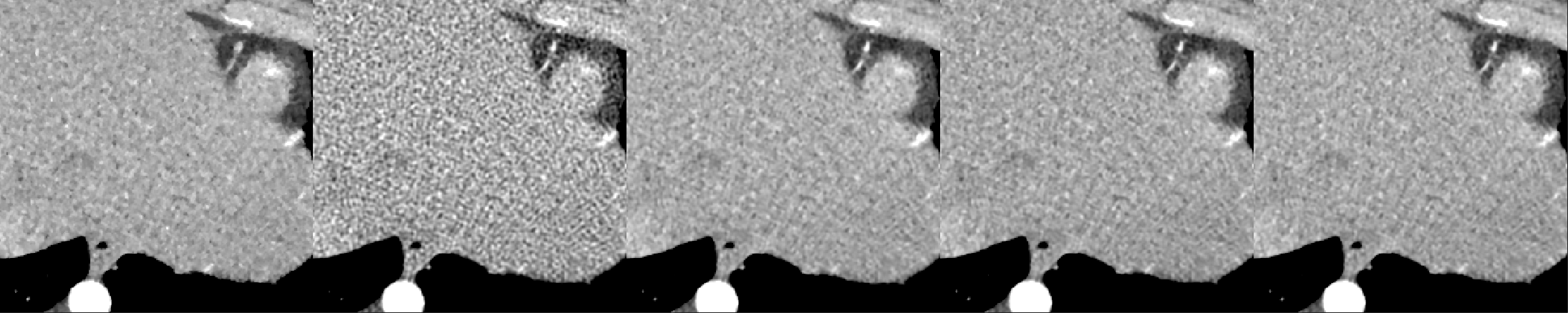
(d)

Figure 3: Reconstructed image. (left to right): $MBIR$, $FBP$, $DL\text{-}MBIR_{1}$, $DL\text{-}MBIR_{3}$, $DL\text{-}MBIR_{5}$. LABEL:sub@fig:Image_10, LABEL:sub@fig:Image_50, LABEL:sub@fig:Image_90 and LABEL:sub@fig:Image_170 represent different slices in the image volume. WW/WL 450/0 HU.

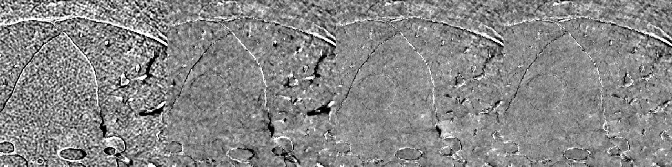
(a)

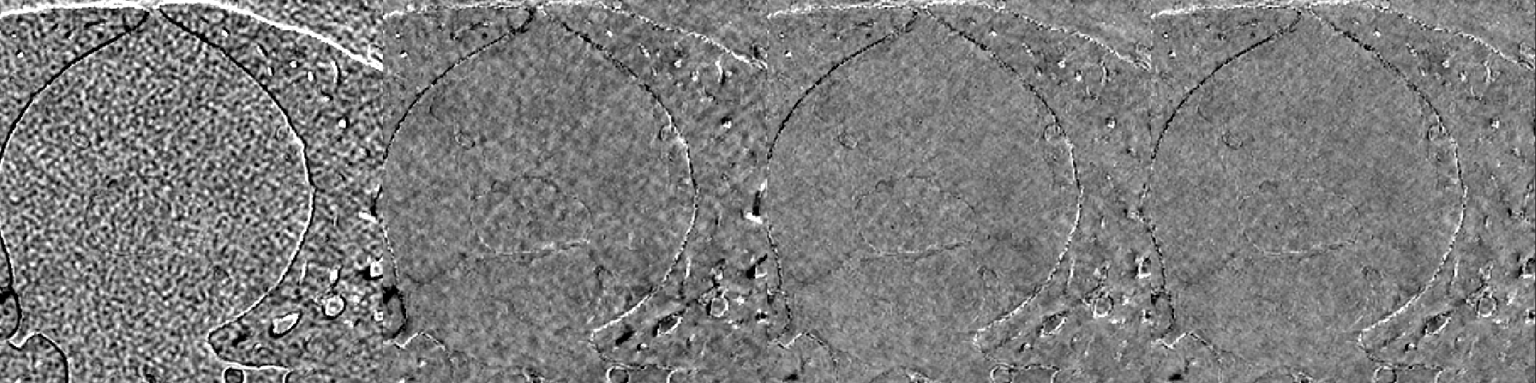
(b)

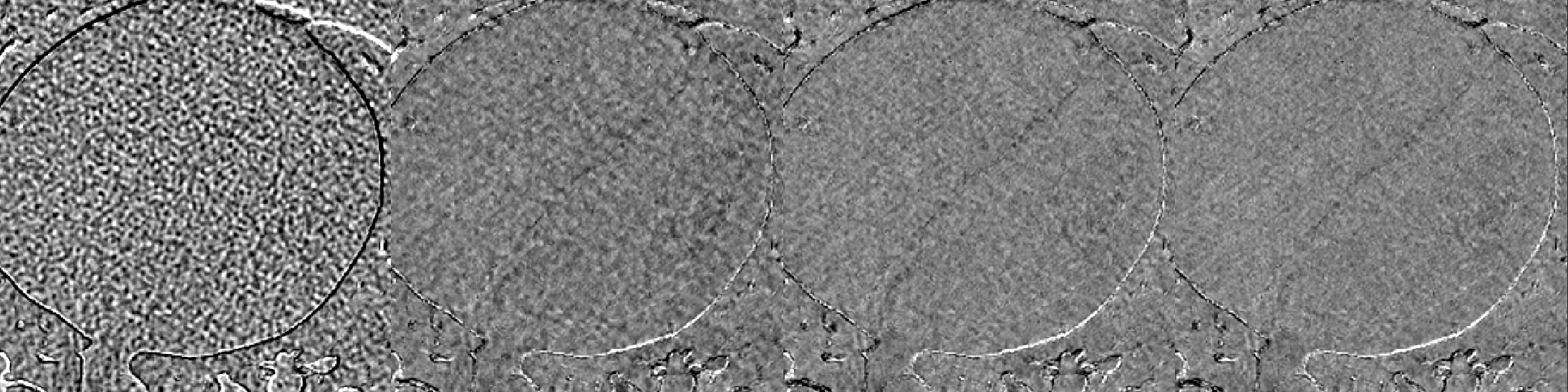
(c)

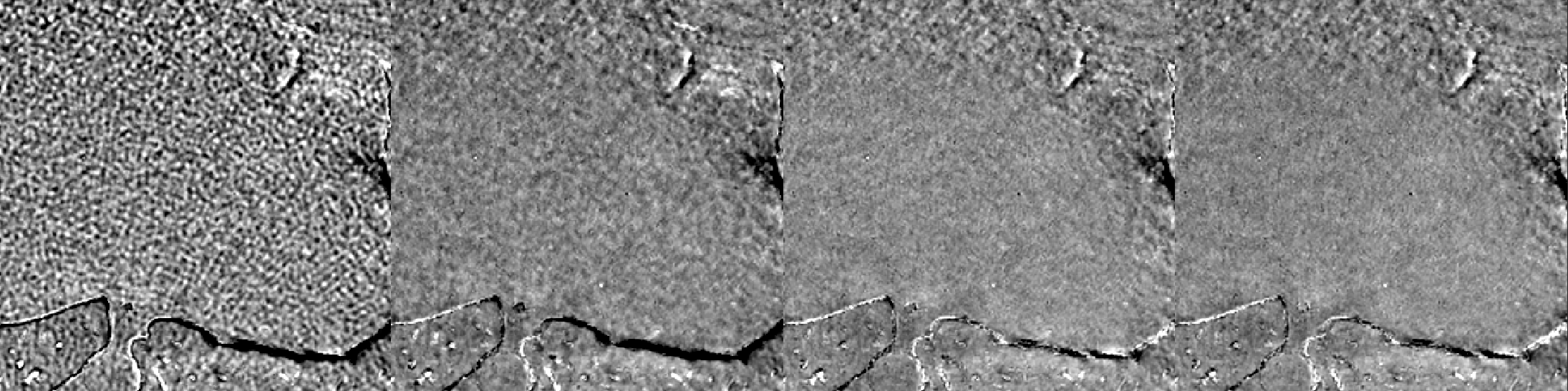
(d)

Figure 4: Difference image w.r.t. MBIR. (left to right): $FBP$, $DL\text{-}MBIR_{1}$, $DL\text{-}MBIR_{3}$, $DL\text{-}MBIR_{5}$. LABEL:sub@fig:Error_10, LABEL:sub@fig:Error_50, LABEL:sub@fig:Error_90 and LABEL:sub@fig:Error_170 represent different slices in the image volume. WW/WL 150/0 HU.

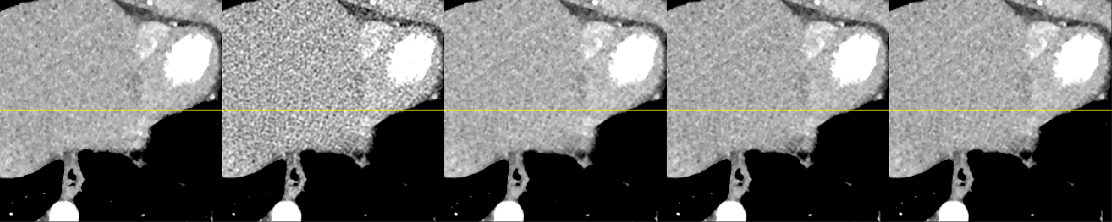
(a)

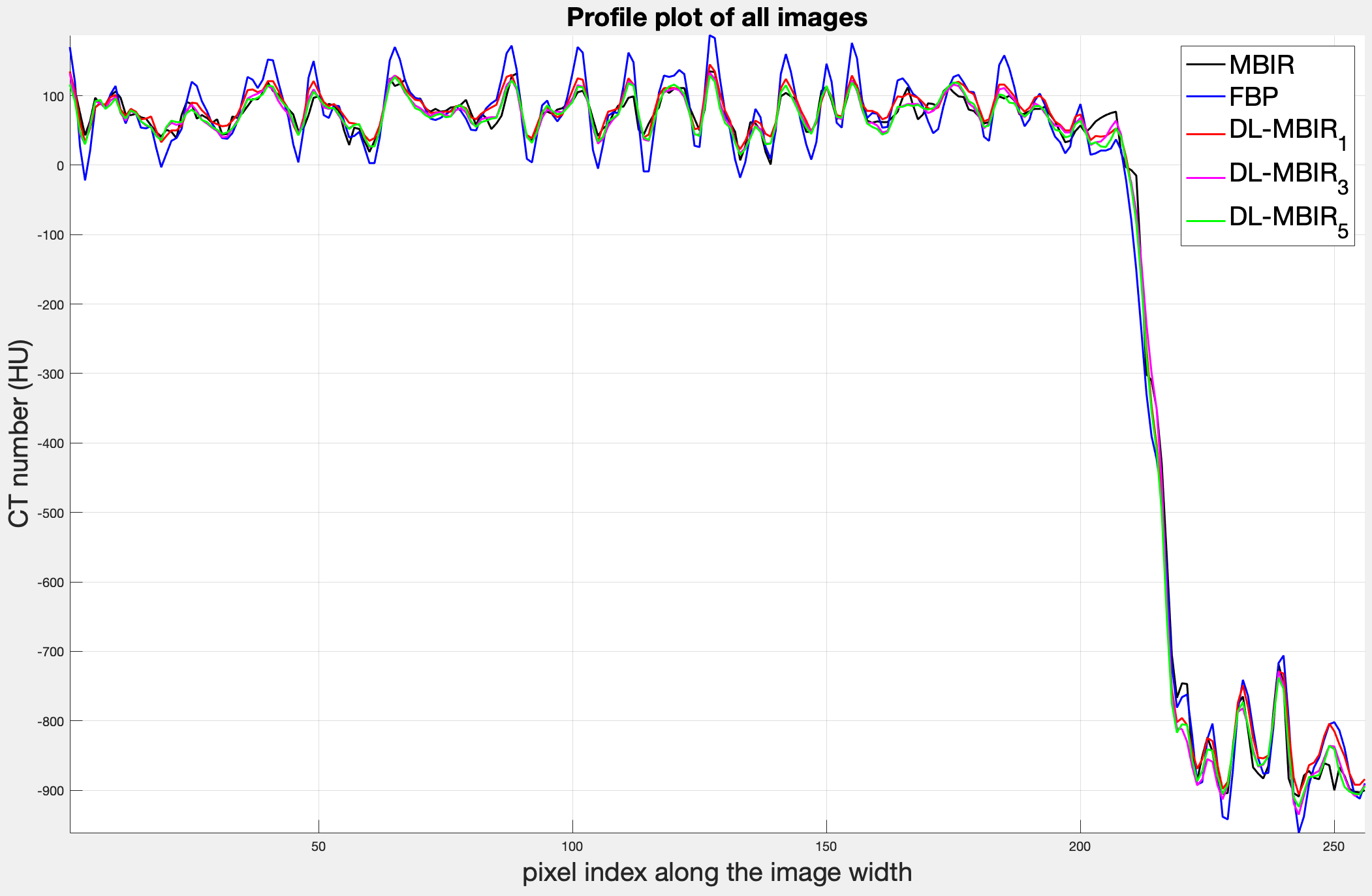
(b)

Figure 5: Image profile. LABEL:sub@fig:Image_160_yline One axial slice, from left to right, of: $MBIR$, $FBP$, $DL\text{-}MBIR_{1}$, $DL\text{-}MBIR_{3}$, $DL\text{-}MBIR_{5}$ LABEL:sub@fig:Profile_160 Profile plot of the images along the yellow line.

	$MBIR$	$FBP$	$DL\text{-}MBIR_{1}$	$DL\text{-}MBIR_{3}$	$DL\text{-}MBIR_{5}$
PSNR	-	64.98	68.99	70.63	71.08
std	25.07	46.65	26.39	27.24	25.85
average	74.68	75.20	77.0	71.52	74.43

Table 1: Performance metrics. PSNR (dB) is calculated w.r.t the MBIR images and averaged for all axial slices. Standard deviation (std) and the average value are in HU, with water being 0 and air -1000.

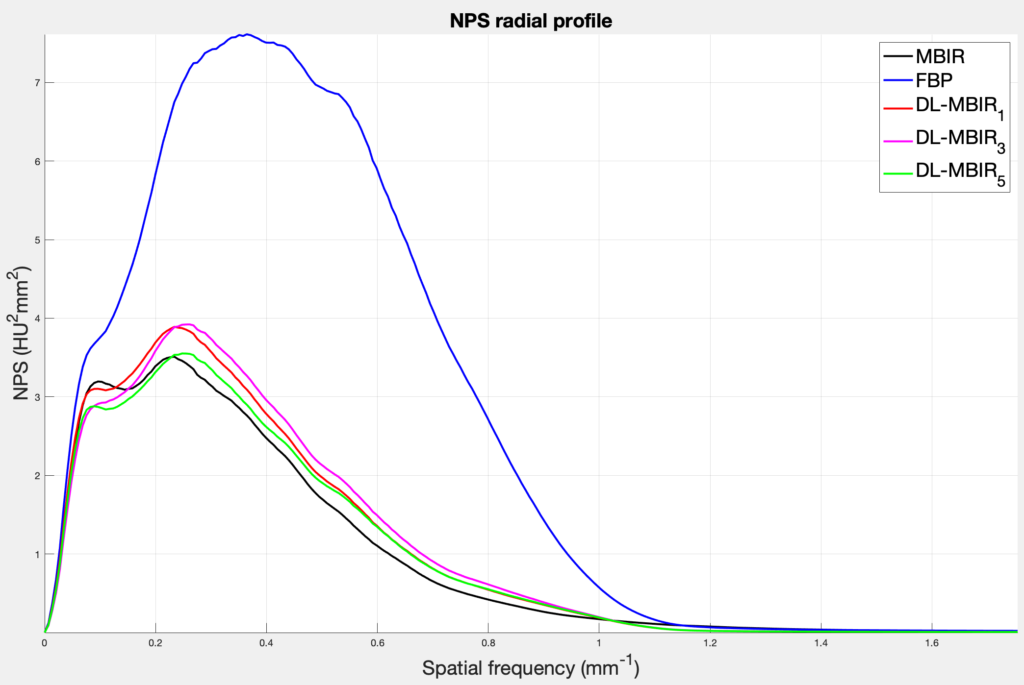
Figure 6: NPS plot demonstrating similar behavior of DL-MBIR with MBIR for noise power.

4 Discussion

Visually, all DL-MBIR images bear close resemblance to the MBIR images in figure 3. It is confirmed by the difference images in figure 4. In the profile plot of Figure 5, the DL-MBIR profiles closely follow that of MBIR.

All DL-MBIR images have higher PSNR than that of FBP, with $DL\text{-}MBIR_{5}$ having the best. Ziabari, et al [7] achieved a PSNR gain over FBP of 3.4 dB for $DL\text{-}MBIR_{1}$, compared to 4.1 dB with the current implementation. For $DL\text{-}MBIR_{5}$, we have improved the result from 4.25 dB to 6.1 dB over FBP. DL-MBIR images have standard deviations nearly the same as MBIR, with $DL\text{-}MBIR_{5}$ outperforming the rest. The average within the chosen RoI is more or less preserved in all images.

In figure 6, noise power spectrum (NPS) plots of DL-MBIR images are quite close to that of MBIR, indicating that the DL-MBIR image texture is also similar to that of MBIR, and it appears this attribute is learned well by the network. Due to its type of adaptive regularization, MBIR may create distinctive texture in the surviving image noise. The attenuation of noise is a clear gain; however this texture and its effect on low-contrast detectability may be of concern to some users.

5 Conclusion

We trained a U-net, 2.5D DL network that effectively estimates MBIR results from FBP input images. The computation cost is also signifcantly less than that of MBIR. All metrics – NPS, PSNR, standard deviation, profile plots demonstrate that DL-MBIR images have all the features of MBIR including noise reduction and noise texture.

References

- [1] Jean-Baptiste Thibault, Ken D Sauer, Charles A Bouman and Jiang Hsieh “A three-dimensional statistical approach to improved image quality for multislice helical CT” In Medical physics 34.11 Wiley Online Library, 2007, pp. 4526–4544
- [2] Zhou Yu et al. “Fast model-based X-ray CT reconstruction using spatially nonhomogeneous ICD optimization” In IEEE Transactions on image processing 20.1 IEEE, 2010, pp. 161–175
- [3] Mingrui Geng et al. “Unsupervised/semi-supervised deep learning for low-dose CT enhancement” In arXiv preprint arXiv:1808.02603, 2018
- [4] Qingsong Yang et al. “Low-dose CT image denoising using a generative adversarial network with Wasserstein distance and perceptual loss” In IEEE transactions on medical imaging 37.6 IEEE, 2018, pp. 1348–1357
- [5] Masakazu Matsuura, Jian Zhou, Naruomi Akino and Zhou Yu “Feature-Aware Deep-Learning Reconstruction for Context-Sensitive X-ray Computed Tomography” In IEEE Transactions on Radiation and Plasma Medical Sciences 5.1 IEEE, 2020, pp. 99–107
- [6] Muhammad Usman Ghani and W Clem Karl “Fast enhanced CT metal artifact reduction using data domain deep learning” In IEEE Transactions on Computational Imaging 6 IEEE, 2019, pp. 181–193
- [7] Amirkoushyar Ziabari et al. “2.5 D deep learning for CT image reconstruction using a multi-GPU implementation” In 2018 52nd Asilomar Conference on Signals, Systems, and Computers, 2018, pp. 2044–2049 IEEE
- [8] Olaf Ronneberger, Philipp Fischer and Thomas Brox “U-net: Convolutional networks for biomedical image segmentation” In International Conference on Medical image computing and computer-assisted intervention, 2015, pp. 234–241 Springer