D-Separation for Causal Self-Explanation

Abstract

Rationalization is a self-explaining framework for NLP models. Conventional work typically uses the maximum mutual information (MMI) criterion to find the rationale that is most indicative of the target label. However, this criterion can be influenced by spurious features that correlate with the causal rationale or the target label. Instead of attempting to rectify the issues of the MMI criterion, we propose a novel criterion to uncover the causal rationale, termed the Minimum Conditional Dependence (MCD) criterion, which is grounded on our finding that the non-causal features and the target label are d-separated by the causal rationale. By minimizing the dependence between the unselected parts of the input and the target label conditioned on the selected rationale candidate, all the causes of the label are compelled to be selected. In this study, we employ a simple and practical measure of dependence, specifically the KL-divergence, to validate our proposed MCD criterion. Empirically, we demonstrate that MCD improves the F1 score by up to $13.7\%$ compared to previous state-of-the-art MMI-based methods. Our code is available at: https://github.com/jugechengzi/Rationalization-MCD.

1 Introduction

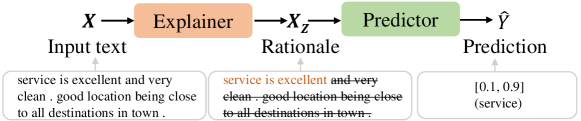
Figure 1: The standard rationalization framework RNP. $X$ is the original full text. $X_{Z}$ is the selected rationale candidate and $\hat{Y}$ is the predictor’s output.

With the success of deep learning, there is growing concern about the interpretability of deep learning models, particularly as they are rapidly being deployed in various critical fields (Lipton, 2018). Ideally, the explanation for a prediction should be both faithful (reflecting the model’s actual behavior) and plausible (aligning with human understanding) (Chan et al., 2022).

Post-hoc explanations, which are trained separately from the prediction process, may not faithfully represent an agent’s decision, despite appearing plausible (Lipton, 2018). Sometimes, faithfulness should be considered a prerequisite that precedes plausibility in explanations of neural networks, especially when these networks are employed to assist in critical decision-making processes, as this factor determines the trustworthiness of the explanations. In contrast to post-hoc methods, ante-hoc (or self-explaining) techniques typically offer increased transparency (Lipton, 2018) and faithfulness (Yu et al., 2021), as the prediction is made based on the explanation itself.

A model-agnostic ante-hoc explanation framework, called Rationalizing Neural Predictions (RNP), was proposed by Lei et al. (2016) and is also known as rationalization. RNP utilizes a cooperative game between an explainer and a predictor, where the explainer identifies a human-interpretable subset of the input (referred to as rationale) and passes it to the subsequent predictor for making predictions, as shown in Figure 1. The explainer and predictor are trained cooperatively to maximize prediction accuracy. A significant advantage of RNP-based rationalization is its certification of exclusion, which guarantees that any unselected part of the input has no contribution to the prediction. This property ensures the maintenance of faithfulness, enabling us to focus solely on plausibility (Yu et al., 2021). Notably, although RNP was initially proposed in the field of NLP and and its enhancement schemes have primarily been validated using text data, its framework can also be applied to other domains, e.g., explaining image classification (Yuan et al., 2022) and graph neural networks (Luo et al., 2020).

Previous rationalization methods generally utilize the maximum mutual information (MMI) criterion to determine the rationale, defined as the subset most indicative of the target label. However, this criterion merely uncovers associations rather than causal relationships between the rationale and the label. Consequently, MMI is easily affected by spurious correlations and the plausibility of chosen rationales might be diminished, even though the rationales still faithfully report the predictor’s behavior (Chang et al., 2020). In rationalization, there are two stages from which correlations may arise. The first type of correlation originates from the process of dataset generation, and we refer to it as feature correlation. A typical example of feature correlation, as pointed out in LIME (Ribeiro et al., 2016), is that wolves often appear together with snow. Consequently, whether the background features snow or not can serve as a strong indicator for classifying an image as depicting a wolf. Another instance of feature correlation is demonstrated in the first row of Table 1. Within a beer review, a favorable taste often correlates with an appealing aroma. Comments regarding the taste can serve as a strong indicator for the smell label. The predictor might inadvertently overfit to such correlations, leading to local optima. Consequently, the suboptimal predictor could mislead the explainer to select these spurious correlations. Another type of correlation stems from the rationale (mask) selection stage, and we call it mask correlation. An example of mask correlation is depicted in the second row of Table 1. Consider a situation where the explainer has implicitly learned the category of $X$, and selects a $``$-$"$ for all negative inputs while excluding it from all positive inputs. In this case, the predictor only needs to determine whether the input rationale includes a $``$-$"$ or not. Even though this phenomenon has not been analyzed from the perspective of spurious correlation, it has been observed and named as degeneration in prior research (Yu et al., 2019).

Some methods have been developed to address either feature correlation or degeneration separately. INVRAT (Chang et al., 2020) attempts to tackle feature correlation using invariant risk minimization (IRM) (Arjovsky et al., 2019). The main idea is to emphasize spurious (non-causal) variations by splitting the dataset into distinct environments. However, IRM-based methods have several limitations. For instance, they require strong prior knowledge about the relationships between non-causal and causal features (e.g., the extra labels of non-causal features) in order to divide the dataset (Lin et al., 2022b). Moreover, IRM-based methods are limited to addressing only a finite set of predetermined non-causal features, neglecting the potential existence of numerous unknown non-causal features. In fact, a recent study (Lin et al., 2022b) in the field of IRM has theoretically demonstrated that it is nearly impossible to partition a dataset into different environments to eliminate all non-causal features using IRM. Other challenges, such as the tendency to overfit, difficulty in applying to larger models (Zhou et al., 2022; Lin et al., 2022a), and the marginal shift risk of the input (Rosenfeld et al., 2021), have also been identified within the realm of IRM. Inter_RAT (Yue et al., 2023) attempts to eliminate feature correlation through backdoor adjustment, intervening directly with the confounders. However, it is extremely hard to measure the confounders since they are usually not observable in the dataset. As for degeneration, although not explicitly associated with spurious correlation until this study, some efforts have been tried to fix the problem. The common idea is to introduce auxiliary modules that have access the full texts to regularize the original explainer (Yu et al., 2021) or the predictor (Yu et al., 2021; Liu et al., 2022). Regularized by these auxiliary modules, the predictor can somewhat disregard the mask correlation, and degeneration is partially alleviated.

Although these methods have tried to fix the problems resulted from spurious correlations, they are still MMI-based methods and how the problems come into being is not well explored. In this study, we first identify the two stages that the spurious correlations may come from, and link the important degeneration problem to a more general mask correlation. Then, we identify that the target label $Y$ and all the non-causal features (including the rationale masks) in the input $X$ are d-separated by the causal features, meaning that the non-causal features are independent of $Y$ given the causal features. This leads to a new avenue for addressing feature correlation and mask correlation simultaneously: we only need to penalize the dependence between the target label and the unselected features conditioned on the selected rationale candidate, such that all the direct causal features will be included in the selected rationale candidate. Based on this observation, we develop a new criterion for the causal rationale, namely minimum conditional dependence (MCD). Various methods can be adopted to measure the dependence, such as mutual information, the Hilbert-Schmidt Independence Criterion (HSIC) (Gretton et al., 2007), and so on. In this paper, we adopt a simple and practical measurement for independence, the KL-divergence, to verify the effectiveness of the proposed criterion. Then, we conduct experiments on two widely used benchmarks to validate the effectiveness of MCD.

Table 1: The examples of feature correlation and mask correlation. Human-annotated rationales are underlined. Rationales from RNP are highlighted in red.

RNP

Dataset: Beer-Aroma.   Label: Positive. Predition: Positive. Problem: feature correlation

Text: the appearance was nice . dark gold with not much of a head but nice lacing when it started to dissipate .  the smell was ever so hoppy with a hint of the grapefruit flavor that ’s contained within .   the taste was interesting , up front tart grapefruit , not sweet in the least . more like grapefruit rind even . $\cdots\cdots.$

Dataset: Beer-Aroma.  Label: Negative. Predition: Negative. Problem: mask correlation

Text: 12 oz bottle poured into a pint glass - a - pours a transparent , pale golden color . the head is pale white with no cream , one finger ’s height , and abysmal retention . i looked away for a few seconds and the head was gone   s - stale cereal grains dominate . hardly any other notes to speak of . very mild in strength t - sharp corn/grainy notes throughout it ’s entirety . $\cdots\cdots.$

In summary, our contributions are:

• To the best of our knowledge, we are the first to identify the degeneration problem as a form of spurious correlation. Leveraging probabilistic graphical models, we are the first to comprehensively elucidate feature correlation and degeneration under a unified perspective.

• We find that the target label and non-causal features are d-separated by the direct causal features. Based on this insight, we propose the MCD criterion, which opens a new avenue for discovering causal rationales, marking the main contribution of this study. Unlike previous methods, MCD-based methods do not require prior expert knowledge about non-causal features, thus presenting potential for broader applicability.

• We present a simple and practical architecture to develop an MCD-based method. Experiments across various datasets demonstrate that our approach achieves an improvement of up to $13.7\%$ in F1 score compared to state-of-the-art MMI-based rationalization methods.

2 Related work

Rationalization. The basic cooperative framework of rationalization called RNP (Lei et al., 2016) is flexible and offers a unique advantage: certification of exclusion, which means any unselected input is guaranteed to have no contribution to the prediction (Yu et al., 2021). Based on this cooperative framework, many methods have been proposed to improve RNP from various aspects. Bao et al. (2018) used Gumbel-softmax to do the reparameterization for binarized selection. Bastings et al. (2019) replaced the Bernoulli sampling distributions with rectified Kumaraswamy distributions. Jain et al. (2020) disconnected the training regimes of the generator and predictor networks using a saliency threshold. Paranjape et al. (2020) imposed a discrete bottleneck objective to balance the task performance and the rationale length. Chang et al. (2019) tried to select class-wise rationales. Antognini et al. (2021); Antognini and Faltings (2021) tried to select rationales belonging to different aspects at once. Zheng et al. (2022) called for more rigorous evaluation of rationalization models. Fernandes et al. (2022) leveraged meta-learning techniques to improve the quality of the explanations. Havrylov et al. (2019) cooperatively trained the models with standard continuous and discrete optimization schemes. Hase et al. (2020) explored better metrics for the explanations. Rajagopal et al. (2021) used phrase-based concepts to conduct a self-explaining model. Other methods like data augmentation with pretrained models (Plyler et al., 2021), training with human-annotated rationales (Chan et al., 2022), have also been tried. These methods are orthogonal to our research.

Spurious correlations. Several methods have been proposed to address the issues arising from either feature correlation or mask correlation. The impact of feature correlation is somewhat mitigated by techniques such as invariant risk minimization (Chang et al., 2020) or backdoor adjustment (Yue et al., 2023). However, as indicated in the introduction, these methods have certain limitations. To combat mask correlation, the usual strategy involves introducing an auxiliary module, which has access to the full input, to regulate the original modules and prevent them from overfitting to trivial patterns introduced by the explainer (Yu et al., 2021, 2019; Liu et al., 2022). Other methods like using multiple explainers to select diverse rationales (Liu et al., 2023a), assigning asymmetric learning rates for the two players (Liu et al., 2023b), have also been tried. Unfortunately, these methods have limited effectiveness against feature correlation in the input data. These aforementioned methods are most relevant to our research, yet we are the first to consider both feature correlation and mask correlation from a unified perspective.

3 Preliminaries

We consider the text classification task, where the input is a text sequence ${X}$=$[x_{1},x_{2},\cdots,x_{l}]$ with ${x}_{i}$ being the $i$-th token and $l$ being the number of tokens. The label of ${X}$ is a one-hot vector $Y\in\{0,1\}^{c}$, where $c$ is the number of categories. $\mathcal{D}$ represents the training set. Ante-hoc rationalization consists of an explainer $f_{E}(\cdot)$ and a predictor $f_{P}(\cdot)$, with $\theta_{e}$ and $\theta_{p}$ representing the parameters of the explainer and predictor, respectively. The goal of an MMI-based explainer is to select the most indicative pieces from the input that are related to the label.

For $(X,Y)\sim\mathcal{D}$, the explainer first outputs a sequence of binary mask $M=f_{E}(X)=[m_{1},\cdots,m_{l}]\in\{0,1\}^{l}$ (in practice, the explainer first outputs a Bernoulli distribution for each token and the mask for each token is independently sampled using gumbel-softmax). Then, it forms the rationale candidate $X_{Z}$ by the element-wise product of $X$ and $M$:

$$X_{Z}=M\odot X=[m_{1}x_{1},\cdots,m_{l}x_{l}].$$ (1)

To simplify the notation, we denote $f_{E}(X)$ as $X_{Z}$ in the following sections, i.e., $f_{E}(X)=X_{Z}$. With the generator’s selection, we get a set of $(Z,Y)$ pairs, which are generally considered to be samples taken from the distribution $P(Z,Y)$. Then, vanilla RNP attempts to identify the rationale by maximizing the mutual information $I(Y;X_{Z})$:

$$X_{Z}^{*}=\mathop{\arg\max}_{X_{Z}}I(Y;X_{Z})=\mathop{\arg\max}_{X_{Z}}(H(Y)-H(Y|X_{Z}))=\mathop{\arg\min}_{X_{Z}}H(Y|X_{Z}),\ s.t.\ X_{Z}=f_{E}(X).$$ (2)

In practice, the entropy $H(Y|X_{Z})$ is commonly approximated by the minimum cross-entropy $\mathop{\min}_{\theta_{p}}H_{c}(Y,\hat{Y}|X_{Z})$, with $\hat{Y}=f_{P}(X_{Z})$ representing the output of the predictor. It is essential to note that the minimum cross-entropy is equal to the entropy (please refer to Appendix B.3). Replacing $X_{Z}$ with $f_{E}(X)$, the explainer and the predictor are trained cooperatively:

$$\mathop{\min}_{\theta_{e},\theta_{p}}H_{c}(Y,f_{P}(f_{E}(X))|f_{E}(X)),\ s.t.,\ (X,Y)\sim\mathcal{D}.$$ (3)

To make the selected rationale human-intelligible, rationalization methods usually constrain the rationales by compact and coherent regularization terms. In this paper, we use the same constraints used in INVRAT (Chang et al., 2020):

$$\Omega(M)=\lambda_{1}\bigg{\lvert}\frac{||M||_{1}}{l}-s\bigg{\rvert}+\lambda_{2}\sum_{t=2}^{l}\big{|}m_{t}-m_{t-1}\big{|}.$$ (4)

The first term encourages that the percentage of the tokens being selected as rationales is close to a pre-defined level $s$. The second term encourages the rationales to be coherent.

4 Method

4.1 Motivation: how spurious correlations come into being.

In this section, we consider $X$ as a set of variables (or a multi-dimensional variables), and the selected rationale candidate $X_{Z}$ is a subset (some dimensions) of it.

To begin with, in Figure 2(a), we posit a probabilistic graphical model to illustrate the corresponding data-generating process for the BeerAdvocate dataset. The input $X$ comprises comments on three aspects: $X_{S}$ for Smell or Aroma, $X_{T}$ for Taste, and $X_{A}$ for Appearance, each of which can be considered as a subset variables of $X$. Additionally, $H$ signifies something that does not discuss the sentiment tendency of $X$. For instance, $H$ could include the color of a bottle. The annotators assign the smell label $Y_{S}$ by viewing the comments on aroma ($X_{S}\xrightarrow{}Y_{S}$). Therefore, only $X_{S}$ serves as the direct cause for $Y_{S}$. However, $X_{S}$ is correlated with $X_{T}$ due to a set of unobserved variables $U$ (called confounders). For example, $U$ may include a variable indicating whether the beer originates from a reputable brand, and a pleasant taste may imply that the beer comes from a good brand ($U\xrightarrow{}X_{T}$). Moreover, a beer from a reputable brand is likely to have a pleasing smell ($U\xrightarrow{}X_{S}$). Consequently, $X_{T}$ is associated with $Y_{S}$ via a backdoor path, as depicted by the red dotted line in Figure 2(a). In this situation, $X_{S}$ is somewhat indicative of $Y_{S}$, but it signifies a statistical correlation rather than causality.

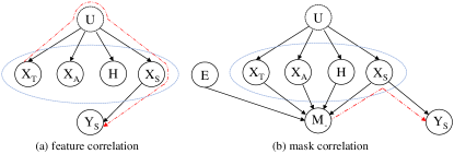
Figure 2: A probabilistic graph for (a) the data generating process of BeerAdvocate and (b) the rationale (mask $M$) selection process.

To have a more intuitive understanding of this correlation, we assume a toy example where $U$, $X_{S}$, $X_{T}$, and $Y_{S}$ are all Bernoulli variables, with their respective probability distributions as:

$$p(U=1)=p(U=0)=0.5,$$ (5)

$$p(X_{T}=1|U=1)=p(X_{T}=0|U=0)=0.9,$$

$$p(X_{S}=1|U=1)=p(X_{S}=0|U=0)=0.9,$$

$$p(Y_{S}=1|X_{S}=1)=p(Y_{S}=0|X_{S}=0)=0.9,$$

With some simple derivations, we can easily obtain (detailed derivation is in Appendix B.1):

$$p(X_{S}=1)=p(X_{T}=1)=p(Y_{S}=1)=0.5.$$ (6)

Then, we can further get (see Appendix B.2 for the detailed derivation of Equation 8 and 9):

$$p(U=1|X_{T}=1)=\frac{p(U=1,X_{T}=1)}{p(X_{T}=1)}=\frac{p(X_{T}=1|U=1)p(U=1)}{p(X_{T}=1)}=0.9.$$ (7)

$$p(X_{S}=1|X_{T}=1)=\sum_{U\in\{0,1\}}p(X_{S}=1|U)p(U|X_{T}=1)=0.9*0.9+0.1*0.1=0.82.$$ (8)

$$p(Y_{S}=1|X_{T}=1)=\sum_{X_{S}\in\{0,1\}}p(Y_{S}=1|X_{S})p(X_{S}|X_{T}=1)=0.82*0.9+0.18*0.1=0.756.$$ (9)

Equation 8 demonstrates that $X_{T}$ (Taste) is highly correlated with $X_{S}$ (Smell), and Equation 9 indicates that $X_{T}$ (Taste) is also strongly indicative of $Y_{S}$ (Smell label). This situation can result in numerous local optima during the rationalization training process. Note that becoming trapped in a local optimum poses a significant challenge in rationalization (Yu et al., 2021; Liu et al., 2022). It is worth noting that the correlation between taste and smell here is merely one of the examples, and sometimes $H$ can also correlate with $Y$ in a similar fashion. For instance, in LIME (Ribeiro et al., 2016), a predictor is trained to determine whether an image contains a wolf or not based on the presence of snow in the background.

Furthermore, the degeneration problem can also be interpreted with a kind of spurious correlation (called mask correlation), as illustrated in Figure 2(b) with an example. Returning to the second example in Table 1, the variable $M_{\_}$, denoting whether $``-"$ is selected as part of the rationale candidate, is caused by the input $X$ (comprising subsets $X_{A}$, $X_{T}$, $X_{S}$ and $H$) and the explainer $E$. $M_{\_}$ is also correlated with $Y_{S}$ through a backdoor path, as indicated by the red line in Figure 2(b).

4.2 The conditional independent property

We first introduce an important concept in probabilistic graphical models, namely d-separation. Subsequently, we demonstrate how d-separation contributes to the identification of causal rationales.

D-Separation (Bishop, 2006): $A$, $B$, and $C$ denote arbitrary, non-intersecting sets of nodes (and their union might not cover all nodes of the graph) in a given probabilistic graph. Our objective is to determine whether a specific conditional independence statement $A\upmodels B|C$ is implied by this graph. To do so, we examine all possible paths from any node in $A$ to any node in $B$. A path is said to be blocked if it includes a node $o$ such that either (see Appendix B.4 for why such a path is blocked)

• (a) The arrows on the path meet at node $o$, forming either a chain (i.e., $\xrightarrow{}o\xrightarrow{}$) or a fork (i.e., $\xleftarrow{}o\xrightarrow{}$), with the node $o$ being part of set C, or

• (b) The arrows on the path meet at node $o$ to form a collider (i.e., $\xrightarrow{}o\xleftarrow{}$), and neither the node $o$ itself nor any of its descendants are included in set C.

If all paths are blocked, then $A$ is considered to be d-separated from $B$ by $C$, meaning that $A\upmodels B|C$.

Returning to our rationalization problem, the backdoor path (dotted red line) in Figure 2(a) comprises a fork ($X_{T}\xleftarrow{}U\xrightarrow{}X_{S}$) and a chain ($U\xrightarrow{}X_{S}\xrightarrow{}Y_{S}$). If either $X_{S}$ or $U$ is included in the conditioning set, the path between $X_{S}$ and $Y_{S}$ becomes blocked, leading to their conditional independence, and consequently, the eradication of corresponding feature correlation. Similarly, the backdoor path (dotted red line) in Figure 2 (b) forms a fork ($M_{-}\xleftarrow{}X_{S}\xrightarrow{}Y_{S}$). By including $X_{S}$ in the conditioning set, the path between $M_{-}$ and $Y_{S}$ is blocked, resulting in their conditional independence and consequently, the elimination of corresponding mask correlation.

We consider the general case, where the input $X$ is a set of variables (or features). $X_{R}$ is a subset of $X$ that exclusively contains all the direct causes of the target label $Y$, i.e., the desiderata of the rationale. We select a subset of $X$ to serve as the rationale candidate (denoted as $X_{Z}$), while the remaining unselected part is referred to as $X_{-Z}$. This leads us to the following properties:

Lemma 1

If $X_{-Z}$ and $Y$ are d-separated by $X_{Z}$, we then have that all of the direct causal features in $X$ must be included in $X_{Z}$:

$$X_{-Z}\ \text{and}\ Y\ \text{are d-separated by}\ X_{Z}\Longrightarrow X_{R}\subset X_{Z}.$$ (10)

The proof is in Appendix B.5. And it’s very easy to intuitively understand it: a direct cause has a one-hop path to the label. To block this path, this cause must be included in $X_{Z}$.

Assumption 1

The label $Y$ has no causal effect on any variables in $X$.

Assumption 1 is naturally valid in most real world applications due to the temporal sequence between $X$ and $Y$. We also provide some failure cases of this assumption in Appendix B.6. Assumption 1 specifies that there is no arrow pointing from $Y$ to any nodes in $X$.

Lemma 2

If Assumption 1 holds, we have:

$$X_{-Z}\ \text{and}\ Y\ \text{are d-separated by}\ X_{Z}\Longleftarrow X_{R}\subset X_{Z}.$$ (11)

The proof is in Appendix B.7. Combining Lemma 1 and Lemma 2, we then have:

Theorem 1

If Assumption 1 holds, then all the direct causal features to $Y$ within $X$ will be included in $X_{Z}$ if and only if $X_{-Z}$ and $Y$ are d-separated by $X_{Z}$:

$$X_{-Z}\ \text{and}\ Y\ \text{are d-separated by}\ X_{Z}\Longleftrightarrow X_{R}\subset X_{Z}.$$ (12)

Remark. In light of Theorem 1, we understand that if we aim to achieve $Y\upmodels X_{-Z}|X_{Z}$, we will consequently incorporate all direct causes of $Y$ into $X_{Z}$. It should be noted that the compactness of $X_{Z}$ is facilitated through the sparsity constraint expressed in Equation 4.

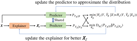
Figure 3: The architecture of our proposed MCD. The approximators for the two distributions are shared to reduce the model complexity.

4.3 The proposed method

Minimum conditional dependence criterion. Although previous research tried to design various auxiliary modules or regularizers to fix the problems of maximum mutual information criterion (Chang et al., 2020; Yue et al., 2023; Liu et al., 2022), we do not follow them to move on this line. Based on Theorem 1, we propose a distinct criterion for identifying the causal rationale, which involves minimizing the dependence between $Y$ and the unselected input $X_{-Z}$, conditioned on $X_{Z}$:

$$X_{Z}^{*}=\mathop{\arg\min}_{X_{Z}}\mathcal{C}(Y,X_{-Z}|X_{Z}),$$ (13)

where $\mathcal{C}$ is a criterion for dependence. For instance, $\mathcal{C}$ could take the form of partial correlation (applicable only to linear associations), mutual information, divergence, or the Hilbert-Schmidt Independence Criterion (HSIC) (Gretton et al., 2007), among others.

It then leads to the question of how we can apply this criterion in practice. In this study, we only present a straightforward and practical method to validate our assertion with respect to Theorem 1, leaving the exploration of other measurements for future work. We first rewrite $Y\upmodels X_{-Z}|X_{Z}$ as

$$P(Y|X_{Z})=P(Y|X_{Z},X_{-Z})=P(Y|X).$$ (14)

Obviously, $P(Y|X_{Z})=P(Y|X)$ if and only if the divergence between the two distributions is zero:

$$Y\upmodels X_{-Z}|X_{Z}\iff P(Y|X_{Z})=P(Y|X)\iff D_{KL}(P({Y|X})||P({Y|X_{Z}}))=0.$$ (15)

Estimating divergence through approximation. The real distributions of $P(Y|X_{Z})$ and $P(Y|X)$ are not directly accessible. So we need further efforts to approximate them. We try to approximate them by making use of the predictor. We first approximate $P(Y|X_{Z})$ with $P(\hat{Y}_{Z}|X_{Z})$ by minimizing the cross-entropy $H_{c}(Y,\hat{Y}_{Z}|X_{Z})$, and we also approximate $P(Y|X)$ with $P(\hat{Y}_{X}|X)$ by minimizing $H_{c}(Y,\hat{Y}_{X}|X)$, where $\hat{Y}_{Z},\hat{Y}_{X}$ are the predictor’s outputs with the inputs being $Z$ and $X$, respectively.

Thus, the training process for our MCD is depicted in Figure 3: the explainer first generates a rationale candidate $X_{Z}$ from the input $X$. Subsequently, $X_{Z}$ and $X$ are fed into the predictor to obtain two distributions, $P(\hat{Y}_{Z}|X_{Z})$ and $P(\hat{Y}_{X}|X)$. By replacing $X_{Z}$ with $f_{E}(X)$ and $\hat{Y}$ with $f_{P}(\cdot)$, the overall objective of our model becomes (The pytorch implementation is in Appendix A.2):

$$\mathop{\min}_{\theta_{p}}E_{(X,Y)\sim\mathcal{D}}[H_{c}(Y,\hat{Y}_{Z}|X_{Z})+H_{c}(Y,\hat{Y}_{X}|X)]$$ (16)

$$+\mathop{\min}_{\theta_{e}}E_{(X,Y)\sim\mathcal{D}}[D_{KL}(P(\hat{Y}_{X}|X)||P(\hat{Y}_{Z}|X_{Z}))+\Omega(M)],$$

$$s.t.,\ X_{Z}=f_{E}(X),\ P(\hat{Y}_{X}|X)=f_{P}(X),\ P({\hat{Y}_{Z}|X_{Z}})=f_{P}(X_{Z}).$$

Notably, although the first term $H_{c}(Y,\hat{Y}_{Z}|X_{Z})$ is similar to the one used in Equation 3, it is detached from the explainer’s parameters $\theta_{e}$. It is now only used to help the predictor approximate the real distribution $P(Y|X_{Z})$ rather than to guide the explainer to find a good rationale.

5 Experiments

5.1 Datasets and metrics

Datasets 1) BeerAdvocate (McAuley et al., 2012) is a multi-aspect sentiment prediction dataset widely adopted in rationalization studies. Given the high correlation among the rating scores of different aspects within the same review, rationale selection encounters severe feature correlation challenges. Following INVRAT (Chang et al., 2020) and Inter_RAT (Yue et al., 2023), we utilize the original dataset (which we refer to as correlated BeerAdvocate) to verify MCD’s effectiveness in handling both feature correlation and mask correlation simultaneously. 2) HotelReviews (Wang et al., 2010) is another multi-aspect sentiment classification dataset containing less feature correlation, which is used by the latest SOTA method FR (Liu et al., 2022) to evaluate the effectiveness of addressing degeneration. We utilize the Service aspect to further demonstrate the competitive edge of our MCD. Among these datasets, each aspect itself can be seen as a dataset and is trained independently.

Metrics. Considering that the annotators assign the label of the target aspect by observing the causal features, the overlap between the tokens selected by the model and those annotated by humans provides a robust metric for rationale causality. The terms $P,R,F1$ denote precision, recall, and $F1$ score respectively. These metrics are the most frequently used in rationalization. The term $S$ represents the average sparsity of the selected rationales, that is, the percentage of selected tokens in relation to the full text. $Acc$ stands for the predictive accuracy.

5.2 Baselines and implementation details

We compare with various recent MMI-based methods that are highly relevant to our study. These include methods like INVRAT (Chang et al., 2020) and Inter_RAT (Yue et al., 2023), which are focused on addressing feature correlation, as well as methods such as FR (Liu et al., 2022) that aim to mitigate mask correlation (i.e., degeneration). Among these, FR represents the latest SOTA approach in addressing mask correlation, while Inter_RAT stands as the SOTA in handling feature correlation.

Both the explainer and the predictor are composed of an encoder (which can be an RNN or Transformer) and a linear layer. Some of the baseline methods have not provided runnable source codes. To ensure a fair comparison, we keep the major settings consistent with those of the baselines, which are commonly utilized in the field of rationalization (Chang et al., 2020; Yu et al., 2021; Liu et al., 2022; Yue et al., 2023). Specifically, we employ the 100-dimensional GloVe (Pennington et al., 2014) for word embedding and 200-dimensional GRUs (Cho et al., 2014) to obtain text representation. The re-parameterization trick for binarized selection is Gumbel-softmax (Jang et al., 2017). The hyperparameters of the reimplemented baselines are initialized with the values reported in their source codes, and are then manually tuned multiple times to determine the optimal settings. We do not use BERT (Devlin et al., 2019) in the main experiments because some recent research (Chen et al., 2022; Liu et al., 2022; Zhang et al., 2022) has found it to be a challenging task to fine-tune large pretrained models within the rationalization framework (see Appendix A.4 for more discussion). However, as a supplement, we also conduct experiments with two pretrained models, ELECTRA (Clark et al., 2020) and BERT. The optimizer is Adam (Kingma and Ba, 2015). All models are trained on a RTX3090 GPU. More details are in Appendix A.1.

Table 2: Results on correlated BeerAdvocate. Each aspect is trained independently. $``*"$: results obtained from Inter_RAT (Yue et al., 2023). The second best F1 scores are underlined.

Methods	Appearance					Aroma					Palate
	S	Acc	P	R	F1	S	Acc	P	R	F1	S	Acc	P	R	F1
RNP∗	10.0	-	32.4	18.6	23.6	10.0	-	44.8	32.4	37.6	10.0	-	24.6	23.5	24.0
INVRAT∗	10.0	-	42.6	31.5	36.2	10.0	-	41.2	39.1	40.1	10.0	-	34.9	45.6	39.5
Inter-RAT∗	11.7	-	66.0	46.5	54.6	11.7	-	55.4	47.5	51.1	12.6	-	34.6	48.2	40.2
FR	11.1	75.8	70.4	42.0	52.6	9.7	87.7	68.1	42.2	52.1	11.7	87.9	43.7	40.9	42.3
MCD(ours)	9.5	81.5	94.2	48.4	63.9	9.9	87.5	84.6	53.9	65.8	9.4	87.3	60.9	47.1	53.1
RNP∗	20.0	-	39.4	44.9	42.0	20.0	-	37.5	51.9	43.5	20.0	-	21.6	38.9	27.8
INVRAT∗	20.0	-	58.9	67.2	62.8	20.0	-	29.3	52.1	37.5	20.0	-	24.0	55.2	33.5
Inter-RAT∗	21.7	-	62.0	76.7	68.6	20.4	-	44.2	65.4	52.8	20.8	-	26.3	59.1	36.4
FR	20.9	84.6	74.9	84.9	79.6	19.5	89.3	58.7	73.3	65.2	20.2	88.2	36.6	59.4	45.3
MCD(ours)	20.0	85.5	79.3	85.5	82.3	19.3	88.4	65.8	81.4	72.8	19.6	87.7	41.3	65.0	50.5
RNP∗	30.0	-	24.2	41.2	30.5	30.0	-	27.1	55.7	36.4	30.0	-	15.4	42.2	22.6
INVRAT∗	30.0	-	41.5	74.8	53.4	30.0	-	22.8	65.1	33.8	30.0	-	20.9	71.6	32.3
Inter-RAT∗	30.5	-	48.1	82.7	60.8	29.4	-	37.9	72.0	49.6	30.4	-	21.8	66.1	32.8
FR	29.6	86.4	50.6	81.4	62.3	30.8	88.1	37.4	75.0	49.9	30.1	87.0	24.5	58.8	34.6
MCD(ours)	29.7	86.7	59.6	95.6	73.4	29.6	90.2	46.1	87.5	60.4	29.4	87.0	30.5	72.4	42.9

5.3 Results

Table 3: Results on HotelReview. $``$*$"$: results obtained from FR (Liu et al., 2022).

Methods	S	Acc	P	R	F1
RNP*	11.0	97.5	34.2	32.9	33.5
DMR*	11.6	-	43.0	43.6	43.3
A2R*	11.4	96.5	37.3	37.2	37.2
FR*	11.5	94.5	44.8	44.7	44.8
MCD(ours)	11.8	97.0	47.0	48.6	47.8

Comparison with SOTA Methods. Table 2 shows the results on correlated BeerAdvocate with the rationale sparsity being about $10\%$, $20\%$, and $30\%$. We set the sparsity to be similar to previous methods by adjusting the sparsity regularization term (i.e., $s$) in Equation 4. Compared to MMI-based methods, we gain significant improvements across all three aspects and three different sparsity. In particular, we improve the F1 score by more then $10\%$ as compared to the previous SOTA in three settings: in the Aroma aspect with $S\approx 10$, the Palate aspect with $S\approx 10$, and the Appearance aspect with $S\approx 30$. We show an visualized example of the selected rationales in Figure 4. Since our MCD criterion (Equation 13) is not limited to a specific measurement of dependence, we also conduct experiments by replacing KL-divergence with JS-divergence, and the results are in Appendix A.5. Table 3 shows the results on another dataset also used in FR, where DMR (Huang et al., 2021) and A2R (Yu et al., 2021) are two recent MMI-based methods. For this dataset, we follow FR to set the sparsity similar to that of the human-annonated rationales. On this dataset, we still beat all the MMI-based methods. We also show the time efficiency in Appendix A.6.

Inducing mask correlation with skewed explainer. In order to evaluate scenarios where feature correlation is not severe and our primary concern is mask correlation, we follow FR’s approach to conduct experiments in a synthetic setting where the explainer is specifically initialized to induce mask correlation, also referred to as degeneration. The details of the initialization can be found in Appendix A.3. Following FR, we utilize the Palate aspect of decorrelated BeerAdvocate dataset (a subset of the original BeerAdvocate that has been filtered by Lei et al. (2016)). This subset contains less feature correlation compared to the original dataset. The results are presented in Table 4, where skew$k$ and $Pre\_acc$ indicates the degree of mask correlation. In this situation, the vanilla RNP fails to identify the causal rationales, and FR is also significantly impacted when the degree of mask correlation is high. Our MCD is much less affected, demonstrating its robustness in such scenarios.

Table 4: Results of skewed explainer that induces degeneration (i.e., mask correlation) in the Palate aspect of BeerAdvocate. $``*"$: results obtained from the paper of FR.

Setting	RNP*						FR*						MCD(ours)
	Pre_acc	S	Acc	R	R	F1	Pre_acc	S	Acc	P	R	F1	Pre_acc	S	Acc	P	R	F1
skew65.0	66.6	14.0	83.9	40.3	45.4	42.7	66.3	14.2	81.5	59.5	67.9	63.4	66.3	12.9	84.6	61.6	63.7	62.6
skew70.0	71.3	14.7	84.1	10.0	11.7	10.8	70.8	14.1	88.3	54.7	62.1	58.1	70.2	13.5	81.1	59.0	64.0	61.4
skew75.0	75.5	14.7	87.6	8.1	9.6	8.8	75.6	13.1	84.8	49.7	52.2	51.0	75.3	13.4	84.2	61.3	65.1	63.1

Table 5: Results of methods using pretrained ELECTRA as the encoder.

Methods	Appearance					Aroma					Plate
	S	Acc	P	R	F1	S	Acc	P	R	F1	S	Acc	P	R	F1
FR-ELECTRA	16.3	86.5	19.1	17.0	18.0	14.8	85.9	58.6	54.8	56.7	11.2	78.0	12.0	10.7	11.3
MCD-ELECTRA	18.5	90.0	84.8	85.6	85.2	14.5	86.6	86.2	78.7	82.3	12.1	85.0	63.0	60.3	61.6

Table 6: The F1 scores of models trained with different encoders. $``$*$"$: results obtained from (Chen et al., 2022). $``$**$"$: results obtained from FR. The dataset is decorrelated Beer-Appearance.

Method	GRU	ELECTRA	BERT
VIB*	-	-	20.5
SPECTRA*	-	-	28.6
RNP**	72.3	13.7	14.7
FR**	82.8	14.6	29.8
MCD(ours)	80.1	85.2	87.1

Experiments with pretrained language models. In the field of rationalization, researchers generally focus on frameworks of the models and the methodology rather than engineering SOTA. The methods most related to our work do not use BERT or other pre-trained encoders (Chang et al., 2020; Yu et al., 2021; Liu et al., 2022; Yue et al., 2023). Experiments in some recent work (Chen et al., 2022; Liu et al., 2022) suggest that there are some unforeseen obstacles making it hard to finetune large pretrained models within the rationalization framework. For example, Table 6 shows that two improved rationalization methods (VIB (Paranjape et al., 2020) and SPECTRA (Guerreiro and Martins, 2021)) and the latest published FR all fail to find the informative rationales when replacing GRUs with pretrained BERT. To eliminate potential factors that could lead to an unfair comparison, we adopt the most widely used GRUs as the encoders in our main experiments, which can help us focus more on substantiating our claims themselves, rather than unknown tricks. But to show the competitiveness of our MCD, we also provide some experiments with pretrained language models as the supplement. Due to limited GPU resources, we adopt the relatively small ELECTRA-small in all three aspects of BeerAdvocate and the relatively large BERT-base in the Appearance aspect. We compare our MCD with the latest SOTA FR (Liu et al., 2022). We follow FR to set the sparsity similar to human-annotated rationales. More details are in Appendix A.4.

The results with BERT are shown in Table 6 and results with ELECTRA are shown in Table 5. We see that our method can greatly benefit from pretrained models. In fact, recent research has found that finetuning large pretrained models can be easily affected by overfitting (Zhang et al., 2021), and spurious correlations can exacerbate this overfitting, particularly in larger models (Zhou et al., 2022; Lin et al., 2022a), which somewhat explains the great progress achieved by our MCD.

Figure 4: An example of selected rationales in the Aroma aspect of BeerAdvocate. The sparsity is set to be about $10\%$. The underlined texts are human-annotated rationales. (a): RNP selects palate only. (b): Inter_RAT selects aroma but also palate ($``$felt very smooth$"$). (c): FR is similar to Inter_RAT. (d): MCD selects aroma only.

6 Conclusion, future work, and limitations

In this study, we first illustrate the two primary issues of feature correlation and degeneration in MMI-based rationalization under a unified causal perspective. Subsequently, we uncover the conditional independence relationship between the target label and non-causal and causal features. Based on this observation, we propose a criterion of minimizing conditional dependence to concurrently address the two aforementioned problems.

Given the versatility of the self-explaining rationalization framework, our proposed methods show significant potential for application across diverse fields such as computer vision and graph learning. Additionally, with the recent remarkable success of large language models (LLMs), exploring how our MCD can aid in training trustworthy LLMs is another avenue worth pursuing.

A potential limitation is that, similar to IRM-based methods, our primary focus is on identifying rationales with causal effects, rather than quantitatively computing the precise values of these causal effects. Although quantifying causality often relies on strong assumptions, this quantification may be a desideratum for certain applications. We aim to explore this direction in future work to accommodate a wider range of applications. Another limitation is that we focus on the text classification task. Different tasks may have very different causal structures. Thus, how to extend this method to other tasks is also a challenge that needs to be explored. The third limitation is that the obstacles in utilizing powerful pretrained language models under the rationalization framework remain mysterious. Although we have made some progress in this direction, we have to say that the empirical results with pretrained models are very sensitive to hyperparameter tuning. A recent paper has also shown that very small changes in hyperparameters can lead to significant differences in results (see Remark 6.1 and Appendix G.2 in (Zhang et al., 2023)). To avoid being distracted by irrelevant factors, until this issue is resolved, we call for research papers to use small models to better verify their claims.

7 Acknowledgements

This work is supported by National Natural Science Foundation of China under grants 62376103, 62302184, 62206102, and Science and Technology Support Program of Hubei Province under grant 2022BAA046. We are also grateful for the valuable suggestions provided by the anonymous reviewers, which greatly helped to improve the quality of this paper.

Appendix A More Results

A.1 More implementation details

To the best of our knowledge, both datasets are sufficiently anonymized to make identification of individuals impossible without significant effort. Both datasets are in English. For correlated BeerAdvocate, we preprocess the data in the same way as Inter_RAT (Yue et al., 2023). For Hotel Reviews, we preprocess them in the same way as FR (Liu et al., 2022). The maximum text length is set to 256. More statistics of the datasets are in Table 7. The dataset of BeerAdvocate is unbalanced. For the training data, we sample from the positive data to get same number of positive and negative texts.

Table 7: Statistics of datasets used in this paper. *: the decorrelated BeerAdvocate.

Datasets		Train		Dev		Annotation
		Pos	Neg	Pos	Neg	Pos	Neg	Sparsity
Beer	Appearance	202385	12897	28488	1318	923	13	18.5
	Aroma	172299	30564	24494	3396	848	29	15.6
	Palate	176038	27639	24837	3203	785	20	12.4
Beer*	Appearance	16891	16891	6628	2103	923	13	18.5
	Aroma	15169	15169	6579	2218	848	29	15.6
	Palate	13652	13652	6740	2000	785	20	12.4
Hotel	Location	7236	7236	906	906	104	96	8.5
	Service	50742	50742	6344	6344	101	99	11.5
	Cleanliness	75049	75049	9382	9382	99	101	8.9

Some previous methods needs very careful hyper-parameter tuning. To make fair comparisons, most results of the baselines are copied from previous papers.

The early stopping technique is conducted according to the predictive accuracy of the development set.

For BeerAdvocate, we use a learning rate of 0.0001 and a batchsize of 128 for our MCD. For HotelReview, we use a learning rate of 0.0001 and a batchsize of 256.

We report the average results of our MDC by running it with five different random seeds.

A.2 Pytorch implementation of Equation 16

For a batch of $(X,Y)$, we first send $X$ to the explainer to get $X_{Z}$:

$$X_{Z}=f_{e}(X).$$ (17)

Then we get a copy of $X_{Z}$ with the pytorch function $``$torch.detach()$"$:

$$X_{Z}^{\prime}=\text{torch.detach}(X_{Z}).$$ (18)

Then, we get $\hat{Y}_{X}$ and $\hat{Y}_{Z}^{\prime}$:

$$\hat{Y}_{X}=f_{p}(X),$$ (19)

$$\hat{Y}_{Z}^{\prime}=f_{p}(X_{Z}^{\prime}).$$

Then we update the predictor with

$$\mathop{\min}_{\theta_{p}}[\text{torch.nn.functional.cross\_entropy}(\hat{Y}_{Z}^{\prime},Y)+\text{torch.nn.functional.cross\_entropy}(\hat{Y}_{X},Y)],$$ (20)

which is the first part of Equation 16. At the same time, we update the explainer with Equation 4.

Now, we deal with the second part of Equation 16. We first freeze the predictor’s parameters and get $X_{Z}$ again:

$$X_{Z}=f_{e}(X).$$ (21)

We now do not copy $X_{Z}$. Instead, we directly get $\hat{Y}_{X}$ and $\hat{Y}_{Z}$:

$$\hat{Y}_{X}=f_{p}(X),$$ (22)

$$\hat{Y}_{Z}=f_{p}(X_{Z}).$$

Then we update the explainer with

$$\min_{\theta_{e}}\text{F.kl\_div}(\text{F.softmax}(\hat{Y}_{Z}).log(),\text{F.softmax}(\hat{Y}_{X})),$$ (23)

where “F” denotes “nn.functional”. In practice, we have added Equation 4 to 23.

Now, an update round for Equation 16 is completed, and we repeat the above steps again.

A.3 Details of the skewed explainer

We pretrain the explainer separately using the text classification label as the mask label of the first token. In other words, for texts of class 1, we force the explainer to select the first token, and for texts of class 0, we force the explainer not to select the first token. So, the explainer learns the category implicitly by whether the first token is chosen and the predictor only needs to learn this position information to make a correct prediction.

$k$ in “skew$k$” denotes the threshold of the skew: we pretrain the explainer as a special classifier of the first token for a few epochs until its prediction accuracy is higher than $k$. Since the accuracy increases rapidly in the first a few epochs, obtaining a model that precisely achieves the pre-defined accuracy is almost impossible. So, we use “$Pre\_acc$” to denote the actual prediction accuracy of the explainer-classifier when the pre-training process stops. Higher “$Pre\_acc$” means easier to degenerate.

A.4 Discussion on BERT encoder

Table 8: Results with BERT. VIB: Paranjape et al. (2020), SPECTRA: Guerreiro and Martins (2021). The results are from Table 4 of (Chen et al., 2022). The metric is F1 score.

Methods	Beer-Appearance	Hotel-Cleanliness
VIB	20.5	23.5
SPECTRA	28.6	19.5

In the field of rationalization, researchers generally focus on frameworks of the models and the methodology. Methods most related to our work do not use Bert or other pre-trained encoders (Chang et al., 2020; Huang et al., 2021; Yu et al., 2019, 2021; Yue et al., 2023). We use GRUs and GloVe to ensure the same experimental setup as our baselines for a fair comparison.

More importantly, how to finetune large models on the rationalization framework is still a significant challenge. Some recent studies (Chen et al., 2022) show that the methods with BERT encoders perform much worse than those with simple GRUs on BeerAdvocate and HotelReviews, which is shown in Table 8. VIB and SPECTRA are two RNP-based models. When using BERT, these two methods perform much worse than the vanilla RNP with GRUs. Table 9 shows the results of a recent workshop paper CR (Zhang et al., 2022), which are also much worse than those with GRUs.

Table 9: The F1 scores of CR (Zhang et al., 2022) with pretrained BERT on BeerAdvocate. The results are from Table 1 of (Zhang et al., 2022).

Method	Appearance	Aroma	Palate
CR	27.4	39.0	22.6

We also conduct experiments with pretrained language models and compare with previous methods. As previous methods are not designed to address feature correlations in the original dataset, they typically utilize the decorrelated BeerAdvocate) dataset where feature correlation is manually filtered by Lei et al. (2016), focusing mainly on mask correlation. Following previous methods (Chen et al., 2022; Liu et al., 2022; Zhang et al., 2022), we use the decorrelated BeerAdvocate dataset. And we set the rationale sparsity to be similar to that of human-annotated rationales. The results are in Table 6 and Table 5.

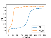
(a) Beer-Appearance

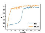
(b) Beer-Aroma

Figure 5: A comparison of convergence speed between our MCD and the latest MMI-based SOTA FR.

A.5 Experiments with JS-divergence

Since our MCD criterion (Equation 13) is not limited to a specific measurement of dependence, we also conduct experiments by replacing KL-divergence with JS-divergence. The results are in Table 10. With either KL-divergence or JS-divergence, our MCD criterion always beat all the MMI-based baselines, showing the effectiveness of MCD.

Table 10: Results on correlated BeerAdvocate. Each aspect is trained independently. $``*"$: results obtained from Inter_RAT (Yue et al., 2023). The second best F1 scores are underlined.

Methods	Appearance					Aroma					Palate
	S	Acc	P	R	F1	S	Acc	P	R	F1	S	Acc	P	R	F1
RNP∗	10.0	-	32.4	18.6	23.6	10.0	-	44.8	32.4	37.6	10.0	-	24.6	23.5	24.0
INVRAT∗	10.0	-	42.6	31.5	36.2	10.0	-	41.2	39.1	40.1	10.0	-	34.9	45.6	39.5
Inter-RAT∗	11.7	-	66.0	46.5	54.6	11.7	-	55.4	47.5	51.1	12.6	-	34.6	48.2	40.2
FR	11.1	75.8	70.4	42.0	52.6	9.7	87.7	68.1	42.2	52.1	11.7	87.9	43.7	40.9	42.3
MCD-KL	9.5	79.7	94.2	48.4	63.9	9.9	87.5	84.6	53.9	65.8	9.4	87.3	60.9	47.1	53.1
MCD-JS	9.7	80.1	95.7	50.2	65.9	10.0	86.1	79.8	51.0	62.2	10.9	85.6	62.1	54.4	58.0
RNP∗	20.0	-	39.4	44.9	42.0	20.0	-	37.5	51.9	43.5	20.0	-	21.6	38.9	27.8
INVRAT∗	20.0	-	58.9	67.2	62.8	20.0	-	29.3	52.1	37.5	20.0	-	24.0	55.2	33.5
Inter-RAT∗	21.7	-	62.0	76.7	68.6	20.4	-	44.2	65.4	52.8	20.8	-	26.3	59.1	36.4
FR	20.9	84.6	74.9	84.9	79.6	19.5	89.3	58.7	73.3	65.2	20.2	88.2	36.6	59.4	45.3
MCD-KL	20.0	85.5	79.3	85.5	82.3	19.3	88.4	65.8	81.4	72.8	19.6	87.7	41.3	65.0	50.5
MCD-JS	19.9	80.8	77.7	83.4	80.5	18.8	87.2	60.5	73.1	66.2	20.2	86.0	42.3	68.5	52.3
RNP∗	30.0	-	24.2	41.2	30.5	30.0	-	27.1	55.7	36.4	30.0	-	15.4	42.2	22.6
INVRAT∗	30.0	-	41.5	74.8	53.4	30.0	-	22.8	65.1	33.8	30.0	-	20.9	71.6	32.3
Inter-RAT∗	30.5	-	48.1	82.7	60.8	29.4	-	37.9	72.0	49.6	30.4	-	21.8	66.1	32.8
FR	29.6	86.4	50.6	81.4	62.3	30.8	88.1	37.4	75.0	49.9	30.1	87.0	24.5	58.8	34.6
MCD-KL	29.7	86.7	59.6	95.6	73.4	29.6	90.2	46.1	87.5	60.4	29.4	87.0	30.5	72.4	42.9
MCD-JS	29.0	89.6	60.2	94.4	73.5	28.7	86.2	47.3	87.0	61.3	27.6	84.5	26.9	59.7	37.1

A.6 Time efficiency

By avoiding many local optima, our MCD can converge much faster than MMI-based methods. Figure 5 shows a comparison of convergence speed between our MCD and the latest MMI-based SOTA FR on Beer-Appearance and Beer-Aroma with $S\approx 20$, where FR and MCD get the similar F1, and they use the same learning rate (0.0001) and batchsize (128).

Appendix B Proofs

B.1 Derivation of Equation 6

We use $X_{S}$ as an example, and the others are nothing different.

$$p(X_{S}=1)=\sum_{U\in\{0,1\}}p(X_{S}=1,U)=\sum_{U\in\{0,1\}}p(X_{S}=1|U)p(U)=0.9*0.5+0.1*0.5=0.5.$$ (24)

B.2 Derivation of Equation 8 and 9

In Figure 2(a), we have $X_{T}\upmodels X_{S}|U$ and $X_{T}\upmodels Y_{S}|X_{S}$ (please refer to Appendix B.4). That is to say,

$$P(X_{S}|U,X_{T})=P(X_{S}|U),\ P(Y_{S}|X_{S},X_{T})=P(Y_{S}|X_{S}).$$ (25)

Then we can easily get Equation 8:

$$p(X_{S}=1|X_{T}=1)= \sum_{U\in\{0,1\}}p(X_{S}=1,U|X_{T}=1)$$ (26)

$$= \sum_{U\in\{0,1\}}p(X_{S}=1|U,X_{T}=1)p(U|X_{T}=1)$$

$$= \sum_{U\in\{0,1\}}p(X_{S}=1|U)p(U|X_{T}=1).$$

And Equation 9 is similar.

B.3 The relation between entropy and cross-entropy

It is a basic idea in information theory that the entropy of a distribution $P$ is upper bounded by the cross entropy of using $Q$ to approximate it. For any two distribution $P$ and $Q$, we have

$$H_{c}(P,Q)=H(P)+D_{KL}(P||Q)\geq H(P),$$ (27)

where the subscript $c$ in $H_{c}(P,Q)$ stands for cross-entropy.

We know that we get the minimum cross entropy when $Q$ is the same as $P$, i.e., $D_{KL}(P||Q)=0$. Which means

$$\mathop{\min}H_{c}(P,Q)=H(P).$$ (28)

B.4 Conditional independence in a probabilistic graph

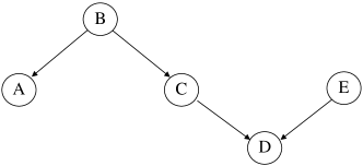
Figure 6: A probabilistic graph that contains a fork, a chain, and a collider.

In the probabilistic graph depicted in Figure 6, we have that $A\upmodels C|B$, $B\upmodels D|C$, and $C\upmodels E$ (but note that we do not have $C\upmodels E|D$). This property is fundamental in probabilistic graphical models. The proof is straightforward, and we illustrate it using $A\upmodels C|B$ as an example.

Based on the general principle of the chain rule, we can have

$$P(A,B,C)= P(C|A,B)P(A,B)$$ (29)

$$= P(C|A,B)P(A|B)P(B).$$

Based on the graph structure in Figure 6, we have

$$P(A,B,C)=P(B)P(A|B)P(C|B)$$ (30)

Combining Equation 29 and 30, we get

$$P(C|B)=P(C|A,B),$$ (31)

which means $A\upmodels C|B$.

If you are seeking a more intuitive understanding of blocked path, please refer to a concept called $``$Bayes ball$"$ (Jordan, 2003).

B.5 Proof of Lemma 1

To prove this, we employ a proof by contradiction. We initially assume that $X_{C}$ is a variable in $X_{R}$ and $X_{C}\notin X_{Z}$. Given that $X_{C}\in X_{R}$, we deduce that $X_{C}$ exerts a direct causal influence on $Y$, i.e., there exists a path $X_{C}\xrightarrow{}Y$:

$$X_{C}\in X_{R}\Longrightarrow X_{C}\xrightarrow{}Y.$$

Furthermore, since $X_{C}\notin X_{Z}$, we ascertain that $X_{C}\in X_{-Z}$. Consequently, we understand that $X_{-Z}$ and $Y$ are not d-separated by $X_{Z}$ due to an unblocked path $X_{C}\xrightarrow{}Y$.

With this, we complete the proof of Lemma 1.

B.6 Failure cases of Assumption 1

As far as we know, most of the real-world datasets are built in a collecting-annotating form. In such a form, $Y$ is given according to $X$, and the annotators won’t edit $X$ after giving $Y$. So, Assumption 1 holds. But there are also some cases that might break Assumption 1. One is the synthetic data like ColorMinist. In ColorMinist, a human first annotates an image, and then edits the image again according to the assigned label. Another scenario is the collection of time series data, where annotators label the data based on existing information and then adjust the data collection method according to the previous labels. This creates a cyclic causal graph. However, in the literature of causal inference, most researchers only consider acyclic graphs. We note that in cases where Assumption 1 doesn’t hold, we still have Lemma 1, i.e., D-separation severs as a sufficient condition for selecting causal rationales. When Assumption 1 holds, it becomes a necessary and sufficient condition.

B.7 Proof of Lemma 2

To prove it, we employ a proof by contradiction. We first assume a variable $X_{C}\in X_{-Z}$, and $X_{C}$ is associated with $Y$ conditioned on $X_{Z}$. To achieve the association, there must be a path in either of the following two forms. The first form is

$$X_{C}\cdots o\xrightarrow{}Y,\quad\ s.t.\ o\notin X_{Z},$$ (32)

where $``\cdots"$ denotes some arbitrary arrows and nodes, and $o$ is a intermediate node. $o\notin X_{Z}$ is from that if $o\in X_{Z}$, the path will be blocked by $X_{Z}$.

Since $o$ is a direct cause of $Y$, we have $o\in X_{R}$. Since $X_{R}\subset X_{Z}$, but we have $o\notin X_{Z}$, so this form of paths do not exist.

The second form is

$$X_{C}\cdots\xrightarrow{}o\xleftarrow{}o_{1}\xleftarrow{}\cdots o_{n}\xleftarrow{}Y,\quad\ s.t.\ o\in X_{Z},$$ (33)

where $o_{1}\cdots o_{n}$ are some nodes connected by left arrows, we do not discuss these nodes since discussing $o$ is enough for our proof.

This path is unblocked through a collider. Note that the way to unblock a collider path is to condition on it, so we need to have $o\in X_{Z}$. However, in this case, $Y$ has a causal effect on $o$, which breaks Assumption 1. So, this form of paths do not exist as well.

As a result, there is no variable in $X_{-Z}$ can be associated with $Y$ conditioned on $X_{Z}$. The proof of Lemma 2 is completed.

References

- Antognini and Faltings (2021) Diego Antognini and Boi Faltings. 2021. Rationalization through concepts. In Findings of the Association for Computational Linguistics: ACL/IJCNLP 2021, Online Event, August 1-6, 2021, volume ACL/IJCNLP 2021 of Findings of ACL, pages 761–775. Association for Computational Linguistics.
- Antognini et al. (2021) Diego Antognini, Claudiu Musat, and Boi Faltings. 2021. Multi-dimensional explanation of target variables from documents. In Thirty-Fifth AAAI Conference on Artificial Intelligence, AAAI 2021, Thirty-Third Conference on Innovative Applications of Artificial Intelligence, IAAI 2021, The Eleventh Symposium on Educational Advances in Artificial Intelligence, EAAI 2021, Virtual Event, February 2-9, 2021, pages 12507–12515. AAAI Press.
- Arjovsky et al. (2019) Martín Arjovsky, Léon Bottou, Ishaan Gulrajani, and David Lopez-Paz. 2019. Invariant risk minimization. CoRR, abs/1907.02893.
- Bao et al. (2018) Yujia Bao, Shiyu Chang, Mo Yu, and Regina Barzilay. 2018. Deriving machine attention from human rationales. In Proceedings of the 2018 Conference on Empirical Methods in Natural Language Processing, Brussels, Belgium, October 31 - November 4, 2018, pages 1903–1913. Association for Computational Linguistics.
- Bastings et al. (2019) Jasmijn Bastings, Wilker Aziz, and Ivan Titov. 2019. Interpretable neural predictions with differentiable binary variables. In Proceedings of the 57th Conference of the Association for Computational Linguistics, ACL 2019, Florence, Italy, July 28- August 2, 2019, Volume 1: Long Papers, pages 2963–2977. Association for Computational Linguistics.
- Bishop (2006) Christopher M. Bishop. 2006. Pattern Recognition and Machine Learning (Information Science and Statistics). Springer-Verlag, Berlin, Heidelberg.
- Chan et al. (2022) Aaron Chan, Maziar Sanjabi, Lambert Mathias, Liang Tan, Shaoliang Nie, Xiaochang Peng, Xiang Ren, and Hamed Firooz. 2022. UNIREX: A unified learning framework for language model rationale extraction. In International Conference on Machine Learning, ICML 2022, 17-23 July 2022, Baltimore, Maryland, USA, volume 162 of Proceedings of Machine Learning Research, pages 2867–2889. PMLR.
- Chang et al. (2019) Shiyu Chang, Yang Zhang, Mo Yu, and Tommi S. Jaakkola. 2019. A game theoretic approach to class-wise selective rationalization. In Advances in Neural Information Processing Systems 32: Annual Conference on Neural Information Processing Systems 2019, NeurIPS 2019, December 8-14, 2019, Vancouver, BC, Canada, pages 10055–10065.
- Chang et al. (2020) Shiyu Chang, Yang Zhang, Mo Yu, and Tommi S. Jaakkola. 2020. Invariant rationalization. In Proceedings of the 37th International Conference on Machine Learning, ICML 2020, 13-18 July 2020, Virtual Event, volume 119 of Proceedings of Machine Learning Research, pages 1448–1458. PMLR.
- Chen et al. (2022) Howard Chen, Jacqueline He, Karthik Narasimhan, and Danqi Chen. 2022. Can rationalization improve robustness? In Proceedings of the 2022 Conference of the North American Chapter of the Association for Computational Linguistics: Human Language Technologies, NAACL 2022, Seattle, WA, United States, July 10-15, 2022, pages 3792–3805. Association for Computational Linguistics.
- Cho et al. (2014) Kyunghyun Cho, Bart van Merrienboer, Çaglar Gülçehre, Dzmitry Bahdanau, Fethi Bougares, Holger Schwenk, and Yoshua Bengio. 2014. Learning phrase representations using RNN encoder-decoder for statistical machine translation. In Proceedings of the 2014 Conference on Empirical Methods in Natural Language Processing, EMNLP 2014, October 25-29, 2014, Doha, Qatar, A meeting of SIGDAT, a Special Interest Group of the ACL, pages 1724–1734. ACL.
- Clark et al. (2020) Kevin Clark, Minh-Thang Luong, Quoc V. Le, and Christopher D. Manning. 2020. ELECTRA: pre-training text encoders as discriminators rather than generators. In 8th International Conference on Learning Representations, ICLR 2020, Addis Ababa, Ethiopia, April 26-30, 2020. OpenReview.net.
- Devlin et al. (2019) Jacob Devlin, Ming-Wei Chang, Kenton Lee, and Kristina Toutanova. 2019. BERT: pre-training of deep bidirectional transformers for language understanding. In Proceedings of the 2019 Conference of the North American Chapter of the Association for Computational Linguistics: Human Language Technologies, NAACL-HLT 2019, Minneapolis, MN, USA, June 2-7, 2019, Volume 1 (Long and Short Papers), pages 4171–4186. Association for Computational Linguistics.
- Fernandes et al. (2022) Patrick Fernandes, Marcos Treviso, Danish Pruthi, André Martins, and Graham Neubig. 2022. Learning to scaffold: Optimizing model explanations for teaching. Advances in Neural Information Processing Systems, 35:36108–36122.
- Gretton et al. (2007) Arthur Gretton, Kenji Fukumizu, Choon Hui Teo, Le Song, Bernhard Schölkopf, and Alexander J. Smola. 2007. A kernel statistical test of independence. In Advances in Neural Information Processing Systems 20, Proceedings of the Twenty-First Annual Conference on Neural Information Processing Systems, Vancouver, British Columbia, Canada, December 3-6, 2007, pages 585–592. Curran Associates, Inc.
- Guerreiro and Martins (2021) Nuno Miguel Guerreiro and André F. T. Martins. 2021. SPECTRA: sparse structured text rationalization. In Proceedings of the 2021 Conference on Empirical Methods in Natural Language Processing, EMNLP 2021, Virtual Event / Punta Cana, Dominican Republic, 7-11 November, 2021, pages 6534–6550. Association for Computational Linguistics.
- Hase et al. (2020) Peter Hase, Shiyue Zhang, Harry Xie, and Mohit Bansal. 2020. Leakage-adjusted simulatability: Can models generate non-trivial explanations of their behavior in natural language? In Findings of the Association for Computational Linguistics: EMNLP 2020, pages 4351–4367.
- Havrylov et al. (2019) Serhii Havrylov, Germán Kruszewski, and Armand Joulin. 2019. Cooperative learning of disjoint syntax and semantics. In Proceedings of the 2019 Conference of the North American Chapter of the Association for Computational Linguistics: Human Language Technologies, NAACL-HLT 2019, Minneapolis, MN, USA, June 2-7, 2019, Volume 1 (Long and Short Papers), pages 1118–1128. Association for Computational Linguistics.
- Huang et al. (2021) Yongfeng Huang, Yujun Chen, Yulun Du, and Zhilin Yang. 2021. Distribution matching for rationalization. In Thirty-Fifth AAAI Conference on Artificial Intelligence, AAAI 2021, Thirty-Third Conference on Innovative Applications of Artificial Intelligence, IAAI 2021, The Eleventh Symposium on Educational Advances in Artificial Intelligence, EAAI 2021, Virtual Event, February 2-9, 2021, pages 13090–13097. AAAI Press.
- Jain et al. (2020) Sarthak Jain, Sarah Wiegreffe, Yuval Pinter, and Byron C. Wallace. 2020. Learning to faithfully rationalize by construction. In Proceedings of the 58th Annual Meeting of the Association for Computational Linguistics, ACL 2020, Online, July 5-10, 2020, pages 4459–4473. Association for Computational Linguistics.
- Jang et al. (2017) Eric Jang, Shixiang Gu, and Ben Poole. 2017. Categorical reparameterization with gumbel-softmax. In 5th International Conference on Learning Representations, ICLR 2017, Toulon, France, April 24-26, 2017, Conference Track Proceedings. OpenReview.net.
- Jordan (2003) Michael Jordan. 2003. An introduction to probabilistic graphical models.
- Kingma and Ba (2015) Diederik P. Kingma and Jimmy Ba. 2015. Adam: A method for stochastic optimization. In 3rd International Conference on Learning Representations, ICLR 2015, San Diego, CA, USA, May 7-9, 2015, Conference Track Proceedings.
- Lei et al. (2016) Tao Lei, Regina Barzilay, and Tommi S. Jaakkola. 2016. Rationalizing neural predictions. In Proceedings of the 2016 Conference on Empirical Methods in Natural Language Processing, EMNLP 2016, Austin, Texas, USA, November 1-4, 2016, pages 107–117. The Association for Computational Linguistics.
- Lin et al. (2022a) Yong Lin, Hanze Dong, Hao Wang, and Tong Zhang. 2022a. Bayesian invariant risk minimization. In IEEE/CVF Conference on Computer Vision and Pattern Recognition, CVPR 2022, New Orleans, LA, USA, June 18-24, 2022, pages 16000–16009. IEEE.
- Lin et al. (2022b) Yong Lin, Shengyu Zhu, Lu Tan, and Peng Cui. 2022b. Zin: When and how to learn invariance without environment partition? Advances in Neural Information Processing Systems, 35:24529–24542.
- Lipton (2018) Zachary C Lipton. 2018. The mythos of model interpretability: In machine learning, the concept of interpretability is both important and slippery. Queue, 16(3):31–57.
- Liu et al. (2023a) Wei Liu, Haozhao Wang, Jun Wang, Ruixuan Li, Xinyang Li, Yuankai Zhang, and Yang Qiu. 2023a. MGR: multi-generator based rationalization. In Proceedings of the 61st Annual Meeting of the Association for Computational Linguistics (Volume 1: Long Papers), ACL 2023, Toronto, Canada, July 9-14, 2023, pages 12771–12787. Association for Computational Linguistics.
- Liu et al. (2022) Wei Liu, Haozhao Wang, Jun Wang, Ruixuan Li, Chao Yue, and YuanKai Zhang. 2022. Fr: Folded rationalization with a unified encoder. In Advances in Neural Information Processing Systems, volume 35. Curran Associates, Inc.
- Liu et al. (2023b) Wei Liu, Jun Wang, Haozhao Wang, Ruixuan Li, Yang Qiu, Yuankai Zhang, Jie Han, and Yixiong Zou. 2023b. Decoupled rationalization with asymmetric learning rates: A flexible lipschitz restraint. In Proceedings of the 29th ACM SIGKDD Conference on Knowledge Discovery and Data Mining, KDD 2023, Long Beach, CA, USA, August 6-10, 2023, pages 1535–1547. ACM.
- Luo et al. (2020) Dongsheng Luo, Wei Cheng, Dongkuan Xu, Wenchao Yu, Bo Zong, Haifeng Chen, and Xiang Zhang. 2020. Parameterized explainer for graph neural network. In Advances in Neural Information Processing Systems 33: Annual Conference on Neural Information Processing Systems 2020, NeurIPS 2020, December 6-12, 2020, virtual.
- McAuley et al. (2012) Julian J. McAuley, Jure Leskovec, and Dan Jurafsky. 2012. Learning attitudes and attributes from multi-aspect reviews. In 12th IEEE International Conference on Data Mining, ICDM 2012, Brussels, Belgium, December 10-13, 2012, pages 1020–1025. IEEE Computer Society.
- Paranjape et al. (2020) Bhargavi Paranjape, Mandar Joshi, John Thickstun, Hannaneh Hajishirzi, and Luke Zettlemoyer. 2020. An information bottleneck approach for controlling conciseness in rationale extraction. In Proceedings of the 2020 Conference on Empirical Methods in Natural Language Processing, EMNLP 2020, Online, November 16-20, 2020, pages 1938–1952. Association for Computational Linguistics.
- Pennington et al. (2014) Jeffrey Pennington, Richard Socher, and Christopher D. Manning. 2014. Glove: Global vectors for word representation. In Proceedings of the 2014 Conference on Empirical Methods in Natural Language Processing, EMNLP 2014, October 25-29, 2014, Doha, Qatar, A meeting of SIGDAT, a Special Interest Group of the ACL, pages 1532–1543. ACL.
- Plyler et al. (2021) Mitchell Plyler, Michael Green, and Min Chi. 2021. Making a (counterfactual) difference one rationale at a time. In Advances in Neural Information Processing Systems 34: Annual Conference on Neural Information Processing Systems 2021, NeurIPS 2021, December 6-14, 2021, virtual, pages 28701–28713.
- Rajagopal et al. (2021) Dheeraj Rajagopal, Vidhisha Balachandran, Eduard H Hovy, and Yulia Tsvetkov. 2021. SELFEXPLAIN: A self-explaining architecture for neural text classifiers. In Proceedings of the 2021 Conference on Empirical Methods in Natural Language Processing, pages 836–850, Online and Punta Cana, Dominican Republic. Association for Computational Linguistics.
- Ribeiro et al. (2016) Marco Túlio Ribeiro, Sameer Singh, and Carlos Guestrin. 2016. "why should I trust you?": Explaining the predictions of any classifier. In Proceedings of the 22nd ACM SIGKDD International Conference on Knowledge Discovery and Data Mining, San Francisco, CA, USA, August 13-17, 2016, pages 1135–1144. ACM.
- Rosenfeld et al. (2021) Elan Rosenfeld, Pradeep Kumar Ravikumar, and Andrej Risteski. 2021. The risks of invariant risk minimization. In 9th International Conference on Learning Representations, ICLR 2021, Virtual Event, Austria, May 3-7, 2021. OpenReview.net.
- Wang et al. (2010) Hongning Wang, Yue Lu, and Chengxiang Zhai. 2010. Latent aspect rating analysis on review text data: a rating regression approach. In Proceedings of the 16th ACM SIGKDD International Conference on Knowledge Discovery and Data Mining, Washington, DC, USA, July 25-28, 2010, pages 783–792. ACM.
- Yu et al. (2019) Mo Yu, Shiyu Chang, Yang Zhang, and Tommi S. Jaakkola. 2019. Rethinking cooperative rationalization: Introspective extraction and complement control. In Proceedings of the 2019 Conference on Empirical Methods in Natural Language Processing and the 9th International Joint Conference on Natural Language Processing, EMNLP-IJCNLP 2019, Hong Kong, China, November 3-7, 2019, pages 4092–4101. Association for Computational Linguistics.
- Yu et al. (2021) Mo Yu, Yang Zhang, Shiyu Chang, and Tommi S. Jaakkola. 2021. Understanding interlocking dynamics of cooperative rationalization. In Advances in Neural Information Processing Systems 34: Annual Conference on Neural Information Processing Systems 2021, NeurIPS 2021, December 6-14, 2021, virtual, pages 12822–12835.
- Yuan et al. (2022) Hao Yuan, Lei Cai, Xia Hu, Jie Wang, and Shuiwang Ji. 2022. Interpreting image classifiers by generating discrete masks. IEEE Transactions on Pattern Analysis and Machine Intelligence, 44(4):2019–2030.
- Yue et al. (2023) Linan Yue, Qi Liu, Li Wang, Yanqing An, Yichao Du, and Zhenya Huang. 2023. Interventional rationalization.
- Zhang et al. (2021) Tianyi Zhang, Felix Wu, Arzoo Katiyar, Kilian Q. Weinberger, and Yoav Artzi. 2021. Revisiting few-sample BERT fine-tuning. In 9th International Conference on Learning Representations, ICLR 2021, Virtual Event, Austria, May 3-7, 2021. OpenReview.net.
- Zhang et al. (2022) Wenbo Zhang, TONG WU, Yunlong Wang, Yong Cai, and Hengrui Cai. 2022. On causal rationalization. In NeurIPS 2022 Workshop on Causality for Real-world Impact.
- Zhang et al. (2023) Wenbo Zhang, Tong Wu, Yunlong Wang, Yong Cai, and Hengrui Cai. 2023. Towards trustworthy explanation: On causal rationalization. In International Conference on Machine Learning, ICML 2023, 23-29 July 2023, Honolulu, Hawaii, USA, volume 202 of Proceedings of Machine Learning Research, pages 41715–41736. PMLR.
- Zheng et al. (2022) Yiming Zheng, Serena Booth, Julie Shah, and Yilun Zhou. 2022. The irrationality of neural rationale models. In Proceedings of the 2nd Workshop on Trustworthy Natural Language Processing (TrustNLP 2022), pages 64–73, Seattle, U.S.A. Association for Computational Linguistics.
- Zhou et al. (2022) Xiao Zhou, Yong Lin, Weizhong Zhang, and Tong Zhang. 2022. Sparse invariant risk minimization. In International Conference on Machine Learning, ICML 2022, 17-23 July 2022, Baltimore, Maryland, USA, volume 162 of Proceedings of Machine Learning Research, pages 27222–27244. PMLR.