Coordinated Multi-Agent Patrolling with History-Dependent Cost Rates - Asymptotically Optimal Policies for Large-Scale Systems

Abstract

We study a large-scale patrol problem with history-dependent costs and multi-agent coordination, where we relax the assumptions on the past patrol studies, such as identical agents, submodular reward functions and capabilities of exploring any location at any time. Given the complexity and uncertainty of the practical situations for patrolling, we model the problem as a discrete-time Markov decision process (MDP) that consists of a large number of parallel restless bandit processes and aim to minimize the cumulative patrolling cost over a finite time horizon. The problem exhibits an excessively large size of state space, which increases exponentially in the number of agents and the size of geographical region for patrolling. We extend the Whittle relaxation and Lagrangian dynamic programming (DP) techniques to the patrolling case, where the additional, non-trivial constraints used to track the trajectories of all the agents are inevitable and significantly complicate the analysis. The past results cannot ensure the existence of patrol policies with theoretically bounded performance degradation. We propose a patrol policy applicable and scalable to the above mentioned large, complex problem. By invoking Freidlin’s theorem, we prove that the performance deviation between the proposed policy and optimality diminishes exponentially in the problem size.

I Introduction

Modern technologies have enabled mission-based agents, such as robots, mobile sensors or unmanned-aerial-vehicles (UAVs), to explore unknown areas with appropriate patrol strategies. The patrolling problems have been studied in a wide range of practical scenarios driven by real-world applications, such as mobile sensor networks in smart cities [1], green security [2], multi-UAV monitoring [3], and emergency response in disasters [4]. Relevant problems have been explored with situational awareness and objectives. For instance, minimization of patrolling costs with persistent agents has been studied in [5, 6], where the cost rate was considered as a function of the visited location and the idle time since last visit to that location. Some other work aimed to maximize the opportunities to capture malicious intruders with moving agents [7, 8].

In this paper, we study patrolling problems with coordinated heterogeneous agents and aim to minimize the cumulative cost, where the cost rates of the patrolled locations are allowed to be history-dependent. The patrolling history of a location can be specified as the idle time since last time this location got patrolled, probabilities of capturing intruders, or some more general and practical history data related to the patrolling process, such as the error covariance matrices of the (non-linear) Kalman filter when gathering information [9, 10, 11].

Past methodologies applicable to relevant problems have been considered through several aspects. Patrolling problems with a single or identical agents have been widely studied for decades [7, 6, 8, 12]. To mitigate the uncertainty of sensing responses, multi-agent patrolling was considered with assumed submodular reward functions [13, 14], where the proposed algorithms were proved to achieve certain approximation ratios. Nonetheless, non-submodularity and/or large numbers of employed agents prevent the techniques from being applied to many practical cases with realistic applications, such as Kalman-filter-based uncertainty mitigation [9, 10]. In [5], a persistent patrolling process was measured by the rewards gained while visiting discretized locations of the patrolled area. The reward function was assumed to be concave and dependent only on the location and the idle time since last visit to that location. In [11, 2], agents (or sensors) were assumed to be able to detect any place at any time without tracking the moving trajectories of the agents and their largest detection coverage. Here, we consider coordinated heterogeneous agents that patrol a large geographical area. We aim to minimize the cumulative costs with practical cost functions that are not necessarily concave or submodular and take consideration of the patrol history of the explored locations.

In [15, 16, 17], multi-agent persistent monitoring problems in an 1-D line were considered with fixed multiple targets and history-dependent target states, aiming at minimizing the uncertainties of the studied systems. The authors proved that, in such a 1-D case, there exist piece-wise linear trajectories, which is optimal for moving the agents. In [18, 17], similar techniques were further discussed for 2-D planes, where the piece-wise linear trajectories are in general sub-optimal, with numerically demonstrated effectiveness of heuristic algorithms. This paper considers similar scenarios except that we allow randomness of both target states and agent trajectories, even if a deterministic algorithm is employed. It enables modeling of more complex detection information of moving targets with unknown or uncertain moving trajectories, other than the binary-style information - detected/monitored and not-detected/non-monitored - of fixed targets.

The coordination of heterogeneous agents, the history-dependent cost rates and the size of the substrate patrolling area substantially complicate the problem and prevent conventional techniques from being applied directly. In this paper, we model the patrolling problem in the vein of the restless multi-armed bandit (RMAB) problem [19]. It follows with well-formulated multi-agent coordination in a dynamic environment, where the high-level idea of the RMAB techniques can be utilized to approximate optimality and to mitigate the curse of dimensionality. In particular, RMAB problem is a Markov decision process (MDP) that consists of parallel bandit processes, each of which, again, is an MDP with binary actions. The RMAB technique has been widely used and discussed in cases where a large number of bandit processes are competing limited opportunities of being selected. The RMAB problem suffers the curse of dimensionality and has been proved to be PSPACE-hard in general [20]. In [19], for the continuous-time RMAB problem, it is conjectured that a simple policy, which was subsequently referred to as the Whittle index policy, approached optimality when the size of the problem tends to infinity. This property is referred to as asymptotic optimality. Later in [21], the conjecture was proved under a non-trivial condition related to the existence of a global attractor of the underlying stochastic process. The non-trivial condition, as well as the asymptotic optimality, has been proved in several different cases [22, 23, 24]. While, in general, it remains an open problem. In [25, 26], discrete-time, finite-time horizon RMAB processes were analyzed through the Lagrangian dynamic programming (DP) technique. Although Lagrangian DP is usually not applicable to continuous-time or infinite time horizon cases, due to its computational complexity increasing polynomially in the number of the discrete time slots, it extends the technique in [19] and leads to proved asymptotic optimality for the discrete-time RMAB problems with finite time horizons.

However, the multi-agent patrolling problem is far from a conventional RMAB process studied in the past [19, 25, 23]. A key difference is the agent-trajectory-dependent constraints over the sets of eligible actions for the next decision epoch. Conventional RMAB processes describe problems of selecting $M$ over $N$ ($N>M$) parallel stochastic processes, each of which can or cannot be selected according to only its own state. While, in the multi-agent patrolling problem, the eligibility of moving an agent to another position is usually dependent on its own position (state), the positions of the other agents (states of other processes), and the overall topology of the patrolling region. It follows with a stronger dependency among the control variables of the parallel stochastic processes, and, when the problem becomes realistically large, the past RMAB results cannot ensure the existence of practical patrol policies with theoretically bounded performance degradation.

The main contributions of this paper are summarized as follows. We model the multi-agent patrolling problem as a set of discrete-time stochastic processes, coupled by inevitable, non-trivial constraints that characterize the dependencies between eligible movements, positions and profiles of the agents. It formulates the coordination of multiple agents and history-dependent cost rates and relaxes the assumptions on the past patrolling models, such as identical agents, submodular reward functions and capability of sensing any location at any time. If we give up the trajectory-dependency by assuming that each agent can be moved to any location at any time, then the patrolling problem reduces to a standard discrete-time RMAB problem. In general, the patrolling problem is complicated by the high-dimensionality of the state space, of which the size increases at least exponentially in the number of agents and the size of the patrolling region.

In the vein of the conventional RMAB problems, we adapt the Whittle relaxation technique [19] and the Lagrangian DP [25] and decompose the patrolling problem, which exhibits the curse of dimensionality, into independent sub-problems with remarkably reduced complexity. We propose a patrolling policy that does not consume excessive computational or storage power when the problem size, measured by the number of agents and locations included in the patrol region, becomes large. This ensures the policy to be scalable, a key attribute to large-scale patrolling problems. The proposed policy quantifies the marginal costs of moving an agent to certain places through real-valued indices and always prioritizes the movements with the least index values. The complexity of implementing the proposed policy is at most linear-logarithmic to the number of agents and quadratic to the size of the patrolling region.

More importantly, by invoking Freidlin’s theorem [27, Chapter 7], we prove that such a policy approaches optimality when the problem size tends to infinity-the policy is asymptotically optimal-and the performance deviation between the proposed policy and optimality diminishes exponentially in the size of the problem. This deviation bound is tighter than the $O(\sqrt{N})$ bound for the standard discrete-time RMAB problem achieved in [25]. Asymptotic optimality and the exponentially-diminishing performance deviation indicate that the proposed policy quickly gets better when the problem becomes larger, and it is appropriate for a large-scale area being explored by many agents.

The theorems achieved in this paper are applicable to a range of optimization problems that care about geographical trajectories along the time line. We demonstrate that Whittle relaxation and Lagrangian DP techniques can be extended to these problems with proved asymptotic optimality and theoretically bounded performance deviation.

The remainder of the paper is organized as follows. In Section II, a description of the patrol model and the underlying stochastic optimization problem is rigorously defined. In Section IV, we propose index policies that are applicable for large-scale systems. We prove in Section V that one of the proposed policies is asymptocially optimal under a mild condition as well as a discussion on the convergence rate of the policy to optimality. The conclusions of this paper are included in Section VI.

II Model

For any positive integer $N$, let $[N]$ represent the set $\{1,2,\ldots,N\}$. Let $\mathbb{R}$, $\mathbb{R}_{+}$ and $\mathbb{R}_{0}$ be the sets of all real numbers, positive real numbers, and non-negative real numbers, respectively. Similarly, $\mathbb{N}$, $\mathbb{N}_{+}$ and $\mathbb{N}_{0}$ are the sets of integers, positive integers and non-negative integers, respectively. Consider a geographical region consisting of $I\in\mathbb{N}_{+}$ different areas and $J\in\mathbb{N}_{+}$ different types of agents. Each type includes $M_{j}\in\mathbb{N}_{+}$, $j\in[J]$, agents that explore all the $I$ areas. Assume that the total number of agents $\sum_{j\in[J]}M_{j}$ is no greater than the number of areas $I$. Agents of the different types can be considered as moving sensors with different functions or profiles, such as cameras and thermal sensors. In each time slot $t\in[T]$ with a finite time horizon $T\in\mathbb{N}_{+}$, each agent, based on the employed patrol policy, moves to another area or stays in the original place and then scans (detects or explores) where it is before next time slot. Consider a limited set of areas, $\mathscr{B}_{i,j}\in 2^{[I]}$, to which an agent of type $j$ can move from the area $i$. We refer to $\mathscr{B}_{i,j}$ as the set of neighbour areas or, alternatively, the neighbourhood of the area $i$ for agent type $j$. For all $i\in[I]$ and $j\in[J]$, assume that $i\in\mathscr{B}_{i,j}$ and $|\mathscr{B}_{i,j}|>1$, indicating that each agent will not be locked in an isolated area. The neighbour areas are determined by intrinsic features of the patrol regime, which can be instantiated as city areas connected by intricate streets, aerial areas being detected by UAVs, wild areas formed by geographical borders, etc. The reachability of a neighbourhood may vary across different agent types due to the maneuverability of different agents. In each time slot, if an area has parked an agent, then other agents of the same type will not explore the same area. That is, agent collision of the same type or repeated sensing within the same time unit is excluded.

For $i\in[I]$, $j\in[J]$ and $t\in[T]$, let a random variable $K_{i,j}(t)$ that takes values in a set $\mathscr{K}_{i,j}$ represent the controller’s knowledge of the area $i$ by the end time slot $t-1$ that was collected or sensed by the agents of type $j$. The value of $K_{i,j}(t)$ can be dependent on the whole patrol and observation history associated with area $i$ and agent type $j$ by time $t$. For example, $K_{i,j}(t)$ may be specified as the idle length by time $t$ since last time area $i$ was visited by an agent of type $j$, the covariance error matrix of (non-linear) Kalman filter by time $t$, the Bayesian probability of detecting an attacker estimated through historical observations by time $t$, et cetera. Recall that $K_{i,j}(t)$ is a random variable, of which the value is affected by the observations (that is, sensing or detecting results within a uncertain environment) before time $t$. Define $I_{i,j}(t)$ as an indicator for the existence of a type-$j$ agent in area $i$ at time $t$. If there is an agent of type $j$ in area $i$ at the end of time slot $t-1$, then $I_{i,j}(t)=1$; otherwise, $0$.

For $i\in[I]$ and $j\in[J]$, define $S_{i,j}(t)\coloneqq(K_{i,j}(t),I_{i,j}(t))$ as the state variable of a stochastic process associated with the area-agent (AA) pair $(i,j)$, and define $\bm{S}(t)\coloneqq(S_{i,j}(t):i\in[I],j\in[J])$. There is a central controller of the patrol problem who makes decisions at each time $t$ based on the value of $\bm{S}(t)$. More precisely, consider an action variable $a_{i,i^{\prime},j}(\bm{S}(t),t)$, a function of the system state $\bm{S}(t)$ and $t$ and taking a value in $\{0,1\}$, for the AA pair $(i,j)$ and an area $i^{\prime}$ ($i,i^{\prime}\in[I]$ and $j\in[J]$). If $a_{i,i^{\prime},j}(\bm{S}(t),t)=1$, then an agent of type $j$ will move to the area $i$ from the area $i^{\prime}$ at the beginning of time $t$ and sense the area before time slot $t+1$; otherwise, no such agent will go from the area $i^{\prime}$ to the area $i$ until next time slot. Note that, if the agent is decided to stay in the area $i$ at both time slots $t$ and $t+1$, then $a_{i,i,j}(\bm{S}(t),t)=1$. Since an agent can move only one step for each time slot, if $i^{\prime}\in[I]\backslash\mathscr{B}_{i,j}$, then $a_{i,i^{\prime},j}(\bm{S}(t),t)\equiv 0$. For an AA pair $(i,j)\in[I]\times[J]$ and time slot $t\in[T]$, define the action vector $\boldsymbol{a}_{i,j}(\bm{S}(t),t)\coloneqq(a_{i,i^{\prime},j}(\bm{S}(t),t):i^{\prime}\in[I])$, and define $\boldsymbol{a}(\bm{S}(t),t)\coloneqq(a_{i,i^{\prime},j}(\bm{S}(t),t):i,i^{\prime}\in[I],j\in[J])$ as the action vector for the entire system. To track the trajectories of the agents, these action variables should satisfy

$$\sum\nolimits_{i^{\prime}\in\mathscr{B}_{i,j}}a_{i,i^{\prime},j}(\bm{S}(t),t)\leq 1,~{}\forall i\in[I],j\in[J],t\in[T],$$ (1)

and

$$\sum\nolimits_{i^{\prime}\in\mathscr{B}_{i,j}}a_{i^{\prime},i,j}(\bm{S}(t),t)=I_{i,j}(t),\forall i\in[I],j\in[J],t\in[T].$$ (2)

Inequality (1) indicates that there is at most one agent of the same type that can move to the same area during the same time slot. The analysis of this entire paper can be directly extended to the case where we allow two or more agents to explore an area simultaneously by changing the constant number at the right hand side of (1) accordingly. Equation (2) guarantees that, for each AA pair $(i,j)$, if there is an agent of type $j$ located in the area $i$ at the end of time slot $t-1$, this agent cannot disappear. It must be moved to an area in the neighbourhood of $i$, including staying at $i$, at the beginning of next time slot. Neither Constraints (1) or (2) match those in conventional RMAB or multi-action bandit models but are essential for our patrol problem.

Example 1: In Figure 1, we consider a simple example with $J=1$ type of agents patrolling $I=36$ areas for crime detection.

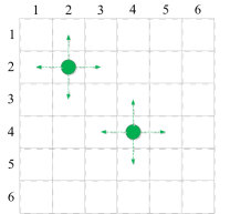
(a) Initialization at the beginning of time slot $t=1$.

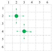
(b) During time slot $t=1$.

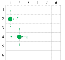
(c) During time slot $t=2$.

Figure 1: An example with $I=36$ areas and $J=1$ type of agents.

Here, each square represents an area with an unknown crime rate $Q_{i}(t)\in[0,1]$, which follows a beta distribution with parameters $(\alpha_{i}(t),\beta_{i}(t))$ ($\alpha_{i}(t),\beta_{i}(t)>0$), at time $t$. If an agent visits area $i$ at time $t$, a random signal $D_{i}(t)$ (taking binary values) is drawn from a Bernoulli distribution with the success probability $Q_{i}(t)$. If $D_{i}(t)=1$, a crime is detected (with probability $Q_{i}(t)$) while patrolling the area $i$ at time $t$; otherwise, nothing happens. After observing the signal $D_{i}(t)$, based on the Bayes’ rule, update the crime rate of area $i$ by setting $(\alpha_{i}(t+1),\beta_{i}(t+1))=(\alpha_{i}(t)+D_{i}(t),\beta_{i}(t)+1-D_{i}(t))$. In this context, $(\alpha_{i}(t),\beta_{i}(t))$ maintains sufficient statistics for measuring the crime rate by time $t$. Let $K_{i,j}(t)=(\alpha_{i}(t),\beta_{i}(t))$, representing the controller’s knowledge of the area $i$ by time $t$, where $j=1$ indicates the only agent type in this example. In Figure 1, the solid green circles represent the agents, the dashed arrows point to the areas the agents can possibly move to, and the solid arrows indicate the actual movements taken by the controller. For the ease of presentation, in this example, we label the area $(x,y)$ (representing the horizontal and vertical axis) in the lattice as $(x-1)*6+y$ ($x,y=1,2,\ldots,6$), and let $M_{1}=2$ (two agents).

In the beginning of time slot $t=1$ (in Figure 1(a)), for AA pairs $(i,j)=(8,1)$ and $(22,1)$, we initialize their states $S_{i,j}(1)=((\alpha_{i},\beta_{i}),1)$ with given $\alpha_{i},\beta_{i}\in\mathbb{R}_{+}$; and, for all the other AA pairs $(i,j)\in[I]\times[J]$, initialize $S_{i,j}(1)=((\alpha_{i},\beta_{i}),0)$. It means that, at the beginning of time slot $t=1$, the two agents are initially located in areas $8$ and $22$, and the controller’s knowledge for all the $36$ areas is $K_{i,j}(1)=(\alpha_{i},\beta_{i})$. Based on $\bm{S}(1)$, the controller decides that $a_{8,8,1}(\bm{S}(1),1)=1$, $a_{21,22,1}(\bm{S}(1),1)=1$, and $a_{i,i^{\prime},j}(\bm{S}(1),1)=0$ for the remaining $i,i^{\prime}\in[I]$. That is, during time slot $t=1$, the controller will keep the agent in area $8$ and move the other agent from area $22$ to $21$, as described in Figure 1(b).

After the agent movement(s) in time slot $t=1$, in the beginning of time slot $t=2$, each agent takes an observation in the located area $i$ ($i=8$ or $21$ in Figure 1(b)) and obtains a signal $D_{i}(1)$. Then, the states of AA pairs $(i,j)=(8,1)$ and $(21,1)$ become $S_{i,j}(2)=((\alpha_{i}+D_{i}(1),\beta_{i}+1-D_{i}(1)),1)$; and, for all the other AA pairs $(i,j)\in[i]\times[J]$, the states variables are $S_{i,j}(2)=((\alpha_{i},\beta_{i}),0)$. Based on the state vector $\bm{S}(2)$, the controller determines the action variables $\bm{a}(\bm{S}(2),2)$, and the agents will be moved accordingly. Consider $a_{7,8,1}(\bm{S}(2),2)=1$, $a_{20,21,1}(\bm{S}(2),2)=1$, and $a_{i,i^{\prime},1}(\bm{S}(2),2)=0$ for all the other $i,i^{\prime}\in[I]$ - moving the agents in areas $8$ and $21$ to $7$ and $20$, respectively, during the time slot $t=2$. Figure 1(c) demonstrates the movements.

Similarly, after the movements in $t=2$, the agents will not move again until $t=3$. In the beginning of slot $t=3$, before taking any movement, the agents will observe their located areas $i\in[I]$, and, based on the observations $D_{i}(3)$, the state vector $\bm{S}(3)$ is again updated. This process continues until reaching the horizon $t=T$.

For $i\in[I]$ and $j\in[J]$, define $\mathscr{S}_{i,j}$ as the set of all the possible values of $S_{i,j}(t)$ ($t\in[T]$), and define the state space of the stochastic process $\{\bm{S}(t),t\in[T]\}$ as $\mathscr{S}\coloneqq\prod_{i\in[I]}\prod_{j\in[J]}\mathscr{S}_{i,j}$, where $\prod$ is the Cartesian product. Recall that each value $s\in\mathscr{S}_{i,j}$ is a tuple, and we rewrite such a tuple as $s=(k(s),\mathcal{i}(s))$. That is, if $S_{i,j}(t)=s$, $k(s)=K_{i,j}(t)$ and $\mathcal{i}(s)=I_{i,j}(t)$. The action vector $\boldsymbol{a}(\cdot,\cdot)$ is in fact a mapping from $\mathscr{S}\times[T]$ to $\{0,1\}^{I^{2}J}$, which determines a policy of the patrol problem. To clarify the dependency between an employed policy, represented by $\phi$, the action variables and the state variables, for any $\boldsymbol{s}\in\mathscr{S}$ and $t\in[T]$, we rewrite $\boldsymbol{a}(\boldsymbol{s},t)$ and $\bm{S}(t)$ as $\boldsymbol{a}^{\phi}(\boldsymbol{s},t)$ and $\bm{S}^{\phi}(t)$, respectively, with the added superscript $\phi$. Similarly, we rewrite $S_{i,j}(t)$, $K_{i,j}(t)$, $I_{i,j}(t)$, $\boldsymbol{a}_{i,j}(\boldsymbol{s},t)$ as $S^{\phi}_{i,j}(t)$, $K^{\phi}_{i,j}(t)$, $I^{\phi}_{i,j}(t)$ and $\boldsymbol{a}^{\phi}_{i,j}(\boldsymbol{s},t)$, respectively. Let $\Phi$ represent the set of all the policies $\phi$ determined by the associated action vector $\boldsymbol{a}^{\phi}$. The process $\{S_{i,j}(t),t\in[T]\}$ associated with each AA pair $(i,j)\in[I]\times[J]$ evolves with different transition probabilities when the area $i$ is or is not explored by an agent of type $j$.

We aim to minimize the cumulative costs of the patrol process $\{\bm{S}^{\phi}(t),t\in[T]\}$ with the objective

$$\min\limits_{\phi\in\Phi}\sum\limits_{t\in[T]}\sum\limits_{i\in[I]}\sum\limits_{j\in[J]}\mathbb{E}\biggl{[}c_{i,j}\Bigl{(}S^{\phi}_{i,j}(t),\mathcal{e}^{\phi}_{i,j}\bigl{(}\bm{S}^{\phi}(t),t\bigr{)},t\Bigr{)}\biggr{]},$$ (3)

subject to (1) and (2), where $\mathcal{e}^{\phi}_{i,j}(\bm{S}^{\phi}(t),t)\coloneqq\mathds{1}\bigl{\{}\sum_{i^{\prime}\in\mathscr{B}_{i,j}}a^{\phi}_{i,i^{\prime},j}(\bm{S}^{\phi}(t),t)>0\bigr{\}}$ indicating whether the area $i$ is explored by an agent of type $j$ at time $t$, $c_{i,j}$ is a non-negative real-valued function representing an instantaneous cost rate, and $\mathbb{E}$ takes expectation over the random variables with a given policy $\phi$ and an initial distribution of $\bm{S}^{\phi}(0)$.

III Lagrangian Dynamic Programming and Relaxation

The problem described in (3), (1) and (2) exhibits a large state space that exponentially increases in the number of agents and the exploring areas. Conventional MDP techniques such as the value iteration cannot achieve optimality without consuming excessively large amount of computational and storage power. We resort to simple heuristic policies that are applicable to large-scale systems and achieve proved near-optimality.

We randomize the action variables and relax (2) to

$$\sum\limits_{i^{\prime}\in\mathscr{B}_{i,j}}\mathbb{E}\Big{[}a^{\phi}_{i^{\prime},i,j}(\bm{S}^{\phi}(t),t)\Bigr{]}=\mathbb{E}\Big{[}I^{\phi}_{i,j}(t)\Big{]},~{}\forall i\in[I],j\in[J],t\in[T],$$ (4)

where the action variables $a^{\phi}_{i,i^{\prime},j}(\bm{S}^{\phi}(t),t)$ take values in $\{0,1\}$ with policy-dependent probabilities. Let $\bar{a}^{\phi}_{i,i^{\prime},j}(\boldsymbol{s},t)\in[0,1]$ ($\boldsymbol{s}\in\mathscr{S}$, $i,i^{\prime}\in[I]$, $j\in[J]$, $t\in[T]$) represent the probability of taking $a^{\phi}_{i,i^{\prime},j}(\boldsymbol{s},t)=1$ under policy $\phi$, and let $\bar{\boldsymbol{a}}^{\phi}_{i,j}(\boldsymbol{s},t)\coloneqq(\bar{a}^{\phi}_{i,i^{\prime},j}(\boldsymbol{s},t):i^{\prime}\in[I])$. In this context, for $i\in[I]$, $j\in[J]$, $t\in[T]$, $\boldsymbol{s}\in\mathscr{S}$, $\phi\in\tilde{\Phi}$ and any $i^{\prime}\in[I]\backslash\mathscr{B}_{i,j}$, $\bar{a}^{\phi}_{i,i^{\prime},j}(\boldsymbol{s},t)\equiv 0$. Define a set $\bar{\Phi}$ of all the policies $\phi$, each of which is determined by $\bar{a}^{\phi}_{i,i^{\prime},j}(\boldsymbol{s},t)$ for all $\boldsymbol{s}\in\mathscr{S}$, $i,i^{\prime}\in[I]$, $j\in[J]$ and $t\in[T]$, and define $\tilde{\Phi}$ as the set of all the policies $\phi\in\bar{\Phi}$ such that, for $(i,j)\in[I]\times[J]$, $\boldsymbol{s}\in\mathscr{S}$, and $t\in[T]$, $\bar{\boldsymbol{a}}^{\phi}_{i,j}(\boldsymbol{s},t)$ takes values in

$$\mathscr{A}_{i,j}\coloneqq\biggl{\{}\boldsymbol{a}\in[0,1]^{I}\biggl{|}\sum\limits_{i^{\prime}\in\mathscr{B}_{i,j}}a_{i^{\prime}}\leq 1\text{ and }a_{i^{\prime}}=0\text{ for all }i^{\prime}\in[I]\backslash\mathscr{B}_{i,j}\biggr{\}}.$$ (5)

Consider the problem

$$\min\limits_{\phi\in\tilde{\Phi}}\sum\limits_{t\in[T]}\sum\limits_{i\in[I]}\sum\limits_{j\in[J]}\mathbb{E}\biggl{[}c_{i,j}\Bigl{(}S^{\phi}_{i,j}(t),\mathcal{e}^{\phi}_{i,j}\bigl{(}\bm{S}^{\phi}(t),t\bigr{)},t\Bigr{)}\biggr{]},$$ (6)

subject to (4). We refer to the problem described in (6) and (4) as the relaxed version of the original problem in (3), (1) and (2). In this context, if a policy $\phi\in\Phi$ is applicable to the original problem (satisfying (1) and (2)), then $\phi\in\tilde{\Phi}$ and is also applicable to the relaxed problem (satisfying (4)). The minimum of the relaxed problem achieves a lower bound for that of the original problem. The dual function of the relaxed problem is

$$L(\boldsymbol{\gamma})=\min\limits_{\phi\in\tilde{\Phi}}\sum\limits_{t\in[T]}\sum\limits_{j\in[J]}\sum\limits_{i\in[I]}\mathbb{E}\biggl{[}c_{i,j}\Bigl{(}S^{\phi}_{i,j}(t),\mathcal{e}^{\phi}_{i,j}\bigl{(}\bm{S}^{\phi}(t),t\bigr{)},t\Bigr{)}+\gamma_{i,j,t}I^{\phi}_{i,j}(t)-\sum\limits_{i^{\prime}\in\mathscr{B}_{i,j}}\gamma_{i^{\prime},j,t}a^{\phi}_{i,i^{\prime},j}(\bm{S}^{\phi}(t),t)\biggr{]},$$ (7)

where $\boldsymbol{\gamma}\in\mathbb{R}^{IJT}$ are the Lagrange multipliers for constraints (4). The right hand side of (7) is the minimized cumulative expected costs of the process $\{\bm{S}^{\phi}(t),t\in[T]\}$ with the expected cost in state $\boldsymbol{s}\in\mathscr{S}$ for action $\boldsymbol{a}=(a_{i,i^{\prime},j}:i,i^{\prime}\in[I],j\in[J])\in\prod_{i\in[I],j\in[J]}\mathscr{A}_{i,j}$ given by

$$C^{\boldsymbol{\gamma}}_{t}(\boldsymbol{s},\boldsymbol{a},t)\coloneqq\sum\limits_{j\in[J]}\biggl{[}\sum\limits_{i\in[I]}\Bigl{(}c_{i,j}\Bigl{(}s_{i,j},\mathcal{e}\bigl{(}\boldsymbol{a}_{i,j}\bigr{)},t\Bigr{)}+\gamma_{i,j,t}\mathcal{i}(s_{i,j})-\sum\limits_{i^{\prime}\in\mathscr{B}_{i,j}}\gamma_{i^{\prime},j,t}a_{i,i^{\prime},j}\Bigr{)}\biggr{]},$$ (8)

where we recall that the action variable $a_{i,i^{\prime},j}\in[0,1]$ represents the probability of moving an agent of type $j$ from the area $i^{\prime}$ to the area $i$, $\boldsymbol{a}_{i,j}\coloneqq(a_{i,i^{\prime},j}:i^{\prime}\in[I])$, $\mathcal{e}(\boldsymbol{a}_{i,j})\coloneqq 1-\prod_{i^{\prime}\in\mathscr{B}_{i,j}}(1-a_{i,i^{\prime},j})$ representing the probability of moving a type-$j$ agent to the area $i$, and, for $e\in(0,1)$, $(i,j)\in[I]\times[J]$, $s\in\mathscr{S}_{i,j}$ and $t\in[T]$, $c_{i,j}(s,e,t)\coloneqq ec_{i,j}(s,1,t)+(1-e)c_{i,j}(s,0,t)$.

III-A Decomposition

For $i\in[I]$, $j\in[J]$ and $\boldsymbol{\gamma}_{i,j}\in\mathbb{R}^{T}$, define

$$L^{\phi}_{i,j}(\boldsymbol{\gamma}_{i,j})\coloneqq\sum\limits_{t\in[T]}\sum\limits_{\boldsymbol{s}\in\mathscr{S}}C^{\boldsymbol{\gamma}_{i,j}}_{i,j}(s_{i,j},\bar{\boldsymbol{a}}^{\phi}_{i,j}(\boldsymbol{s},t),t)\mathbb{P}\Bigl{\{}\bm{S}^{\phi}(t)=\boldsymbol{s}\Bigr{\}},$$ (9)

where, for $s\in\mathscr{S}_{i,j}$ and $\boldsymbol{a}\in\mathscr{A}_{i,j}$,

$$C^{\boldsymbol{\gamma}_{i,j}}_{i,j}(s,\boldsymbol{a},t)\coloneqq c_{i,j}(s,\mathcal{e}(\boldsymbol{a}),t)+\gamma_{i,j,t}\mathcal{i}(s)-\sum\limits_{i^{\prime}\in\mathscr{B}_{i,j}}\gamma_{i^{\prime},j,t}a_{i^{\prime}}.$$ (10)

Equation (7) can be rewritten as

$$L(\boldsymbol{\gamma})=\min\nolimits_{\phi\in\tilde{\Phi}}\sum\limits_{i\in[I]}\sum\limits_{j\in[J]}L^{\phi}_{i,j}(\boldsymbol{\gamma}_{i,j}),$$ (11)

where $\boldsymbol{\gamma}=(\gamma_{i,j,t}:i\in[I],j\in[J],t\in[T])$ and $\boldsymbol{\gamma}_{i,j}=(\gamma_{i,j,t}:t\in[T])$. We refer to the MDP $\{S^{\phi}_{i,j}(t),t\in[T]\}$ as the sub-process $(i,j)$.

Following the idea of Whittle relaxation in [19], there is no constraint that restricts the value of each $L^{\phi}_{i,j}(\boldsymbol{\gamma}_{i,j})$ at the right hand side of (11) once the others are known. More precisely, consider the following proposition.

Proposition 1

For given $\boldsymbol{\gamma}\in\mathbb{R}^{IJT}$,

$$L(\boldsymbol{\gamma})=\min\limits_{\phi\in\tilde{\Phi}}\sum\limits_{i\in[I]}\sum\limits_{j\in[J]}L^{\phi}_{i,j}(\boldsymbol{\gamma}_{i,j})=\sum\limits_{i\in[I]}\sum\limits_{j\in[J]}\min\limits_{\phi_{i,j}\in\tilde{\Phi}}L^{\phi_{i,j}}_{i,j}(\boldsymbol{\gamma}_{i,j}),$$ (12)

where $\boldsymbol{\gamma}_{i,j}=(\gamma_{i,j,t}:t\in[T])$.

The proof of Proposition 1 is provided in Appendix A.

Observe that the minimization over $\phi\in\tilde{\Phi}$ for each $L^{\phi}_{i,j}(\boldsymbol{\gamma}_{i,j})$ in (12) is equivalent to choosing the value of

$$\alpha^{\phi}_{i,i^{\prime},j}(s,t)\coloneqq\mathbb{E}\Bigl{[}a^{\phi}_{i,i^{\prime},j}(\bm{S}^{\phi}_{i,j}(t),t)~{}|~{}S^{\phi}_{i,j}(t)=s\Bigr{]}$$ (13)

in $[0,1]$ for all $i\in[I]$, $s\in\mathscr{S}_{i,j}$ and $t\in[T]$. The value of $\alpha^{\phi}_{i,i^{\prime},j}(s,t)$ is considered as the probability of moving an agent of type $j$ from area $i^{\prime}$ to area $i$ at time $t$ under policy $\phi$, given $S^{\phi}_{i,j}(t)=s$. The minimization over $\phi\in\tilde{\Phi}$ in the dual function can be decomposed into $IJ$ independent sub-problems. We refer to $\min_{\phi\in\tilde{\Phi}}L^{\phi}_{i,j}(\boldsymbol{\gamma}_{i,j})$ as the sub-problem $(i,j)$. Compared to the original problem, the state space of each sub-problem has been significantly reduced.

For given $\boldsymbol{\gamma}_{i,j}\in\mathbb{R}^{T}$ and $(i,j)\in[I]\times[J]$, define $V^{\boldsymbol{\gamma}_{i,j}}_{i,j}(s,t)$ ($s\in\mathscr{S}_{i,j},t\in[T]$) as the solution of the Bellman equations

$$V^{\boldsymbol{\gamma}_{i,j}}_{i,j}(s,t)=\min\limits_{\boldsymbol{a}\in\mathscr{A}_{i,j}}\Bigl{\{}C^{\boldsymbol{\gamma}_{i,j}}_{i,j}(s,\boldsymbol{a},t)+\sum\limits_{s^{\prime}\in\mathscr{S}_{i,j}}P_{i,j,t}(s,\mathcal{e}(\boldsymbol{a}),s^{\prime})V^{\boldsymbol{\gamma}_{i,j}}_{i,j}(s^{\prime},t+1)\Bigr{\}},~{}\forall s\in\mathscr{S}_{i,j},t\in[T],$$ (14)

where recall that, for $\boldsymbol{a}=(a_{i^{\prime}}:i^{\prime}\in[I])\in\mathscr{A}_{i,j}$, $\mathcal{e}(\boldsymbol{a})=1-\prod_{i^{\prime}\in\mathscr{B}_{i,j}}(1-a_{i^{\prime}})$ representing the probability of moving a type-$j$ agent to the area $i$ under the action $\boldsymbol{a}$, $V^{\boldsymbol{\gamma}_{i,j}}_{i,j}(s,T+1)\equiv 0$ for all $s\in\mathscr{S}_{i,j}$, and $P_{i,j,t}(s,\mathcal{e}(\boldsymbol{a}),s^{\prime})$ are the transition probabilities from state $s$ to $s^{\prime}$. For $\mathcal{e}(\boldsymbol{a})=0$ or $1$, the transition probabilities $P_{i,j,t}(s,\mathcal{e}(\boldsymbol{a}),s^{\prime})$ are given values, determined by the intrinsic properties of the AA pair $(i,j)$. While $P_{i,j,t}(s,\mathcal{e}(\boldsymbol{a}),s^{\prime})$ for $\mathcal{e}(\boldsymbol{a})\in(0,1)$ is a linear combination of the former probabilities; that is, for $\mathcal{e}(\boldsymbol{a})=e\in(0,1)$, $P_{i,j,t}(s,e,s^{\prime})=eP_{i,j,t}(s,1,s^{\prime})+(1-e)P_{i,j,t}(s,0,s^{\prime})$. We can solve (14) for all $(i,j)\in[I]\times[J]$ independently. From [28], there exists an optimal solution $\phi^{*}$ for sub-problem $(i,j)$ satisfying that, for any $s\in\mathscr{S}_{i,j}$ and $t\in[T]$, $\alpha^{\phi^{*}}_{i,i^{\prime},j}(s,t)=a_{i^{\prime}}$ where $\boldsymbol{a}\in\mathscr{A}_{i,j}$ minimizes the right hand side of (14). We refer to $V^{\boldsymbol{\gamma}_{i,j}}_{i,j}(s,t)$ ($s\in\mathscr{S}_{i,j}$ and $t\in[T+1]$) as the value function of sub-problem $(i,j)$ for given $\boldsymbol{\gamma}_{i,j}$.

The dual version of the relaxed problem described in (6) and (4) is

$$\max\limits_{\boldsymbol{\gamma}\in\mathbb{R}^{IJT}}L(\boldsymbol{\gamma})=\max\limits_{\boldsymbol{\gamma}\in\mathbb{R}^{IJT}}\sum\limits_{i\in[I]}\sum\limits_{j\in[J]}\min\limits_{\phi\in\tilde{\Phi}}L^{\phi}_{i,j}(\boldsymbol{\gamma}_{i,j}),$$ (15)

where the equality is achieved based on (12). For $(i,j)\in[I]\times[J]$ and given probability $\pi^{0}_{i,j}(s)$ of the initial state $S^{\phi}_{i,j}(1)=s$, $\min_{\phi\in\tilde{\Phi}}L^{\phi}_{i,j}(\boldsymbol{\gamma}_{i,j})=\sum_{s\in\mathscr{S}_{i,j}}\pi^{0}_{i,j}(s)V^{\boldsymbol{\gamma}_{i,j}}_{i,j}(s,1)$. Since $V^{\boldsymbol{\gamma}_{i,j}}_{i,j}(s,t)$ ($s\in\mathscr{S}_{i,j}$ and $t\in[T]$) are the solutions of the equations described in (14), the problem in (15) achieves the same maximum as

$$\max\nolimits_{\begin{subarray}{~{}}\boldsymbol{\gamma}\in\mathbb{R}^{IJT},\\ \bm{V}\in\mathbb{R}^{N}\end{subarray}}\sum\limits_{i\in[I]}\sum\limits_{j\in[J]}\sum\limits_{s\in\mathscr{S}_{i,j}}\pi^{0}_{i,j}(s)V_{i,j}(s,1)$$ (16)

subject to

$$V_{i,j}(s,t)\leq C^{\boldsymbol{\gamma}_{i,j}}_{i,j}(s,\boldsymbol{\alpha},t)+\sum\limits_{s^{\prime}\in\mathscr{S}_{i,j}}P_{i,j,t}(s,\mathcal{e}(\boldsymbol{\alpha}),s^{\prime})V_{i,j}(s^{\prime},t+1),~{}\forall i\in[I],j\in[J],t\in[T],s\in\mathscr{S}_{i,j},\boldsymbol{\alpha}\in\tilde{\mathscr{A}}_{i,j},$$ (17)

and

$$V_{i,j}(s,T+1)=0,~{}\forall i\in[I],j\in[J],s\in\mathscr{S}_{i,j},$$ (18)

where $\tilde{\mathscr{A}}_{i,j}\coloneqq\{0,1\}^{I}\cap\mathscr{A}_{i,j}$, $\pi^{0}_{i,j}(s)$ is the given probability of the initial state $s\in\mathscr{S}_{i,j}$, $V_{i,j}(s,t)$ ($i\in[I],j\in[J],t\in[T],s\in\mathscr{S}_{i,j}$) and $\boldsymbol{\gamma}$ are the unknown variables, and $\bm{V}\coloneqq(V_{i,j}(s,t):i\in[I],j\in[J],s\in\mathscr{S}_{i,j},t\in[T+1])$ with cardinality $N=(T+1)\sum_{(i,j)\in[I]\times[J]}|\mathscr{S}_{i,j}|$. Let $\boldsymbol{\gamma}^{*}\in\mathbb{R}^{IJT}$ and $\bm{V}^{*}\in\mathbb{R}^{N}$ represent an optimal solution of (16)-(18). For any $(i,j)\in[I]\times[J]$, $t\in[T]$ and $s\in\mathscr{S}_{i,j}$, $V^{*}_{i,j}(s,t)=V^{\boldsymbol{\gamma}^{*}_{i,j}}_{i,j}(s,t)$, where $\boldsymbol{\gamma}^{*}_{i,j}=(\gamma^{*}_{i,j,t}:t\in[T])$.

The linear optimization described in (16)-(18) includes $(T+1)\sum_{(i,j)\in[I]\times[J]}|\mathscr{S}_{i,j}|+IJT$ unknown variables that can be obtained by conventional linear programming methods, such as the interior point methods [29, 30] and sub-gradient descent. Recall that this linear optimization is different from the original patrolling problem in (3), (1) and (2), for which an optimal solution is achievable but, in general, not applicable to the original problem. Solving the linear optimization is an intermediate step for proposing a near-optimal scheduling policy for the original problem. We provide in Section IV-A the detailed steps of proposing such a scheduling policy and, in Section IV-B, analysis on its computational complexity.

III-B Strong Duality

We prove in this subsection that the complementary slackness gap between optimality of the primary and dual problems becomes zero under a threshold policy. That is, this threshold policy achieves optimality of the relaxed problem described in (6) and (4). The threshold policy is in general not applicable to the original patrol problem described in (3), (1) and (2), but it quantifies marginal costs of moving agents to different directions. Based on quantified marginal costs, in Section IV, we propose a heuristic policy that is scalable and applicable to the original patrol problem, and, in Section V-A, we prove that this heuristic policy is near-optimal.

Lemma 1 (Indexability)

For $i\in[I]$, $j\in[J]$, and $\boldsymbol{\gamma}_{i,j}\in\mathbb{R}^{T}$, a policy $\phi_{i,j}(\boldsymbol{\gamma}_{i,j})\in\tilde{\Phi}$ is optimal to $\min\nolimits_{\phi_{i,j}\in\tilde{\Phi}}L^{\phi}_{i,j}(\boldsymbol{\gamma}_{i,j})$ (the sub-problem $(i,j)$) if, for $t\in[T]$, $i^{\prime}\in\mathscr{B}_{i,j}$ and $s\in\mathscr{S}_{i,j}$,

$$\alpha^{\phi_{i,j}(\boldsymbol{\gamma}_{i,j})}_{i,i^{\prime},j}(s,t)\left\{\begin{array}[]{ll}=1,&\text{if }\gamma_{i^{\prime},j,t}>\vartheta^{\boldsymbol{\gamma}_{i,j}}_{i,j}(s,t)\text{ and }i^{\prime}=\min\arg\max\limits_{i^{\prime\prime}\in\mathscr{B}_{i,j}}\gamma_{i^{\prime\prime},j,t},\\ \in[0,1],&\text{if }\gamma_{i^{\prime},j,t}=\vartheta^{\boldsymbol{\gamma}_{i,j}}_{i,j}(s,t)\text{ and }\gamma_{i^{\prime},j,t}=\max\limits_{i^{\prime\prime}\in\mathscr{B}_{i,j}}\gamma_{i^{\prime\prime},j,t},\\ =0,&\text{otherwise},\end{array}\right.$$ (19)

where

$$\vartheta^{\boldsymbol{\gamma}_{i,j}}_{i,j}(s,t)\coloneqq c_{i,j}(s,1,t)-c_{i,j}(s,0,t)+\sum\limits_{s^{\prime}\in\mathscr{S}_{i,j}}\Bigl{(}P_{i,j,t}(s,1,s^{\prime})-P_{i,j,t}(s,0,s^{\prime})\Bigr{)}V^{\boldsymbol{\gamma}_{i,j}}_{i,j}(s^{\prime},t+1).$$ (20)

The proof of Lemma 1 is provided in Appendix B.

Lemma 1 implies that the optimal solution for each sub-problem exists in a threshold form (19), similar to the Whittle indexability for a standard RMAB problem. For a continuous-time RMAB problem, the discussion of Whittle indexability remains an open question in general, and it has been proved under non-trivial conditions in [31, 32, 33]. While, for the discrete-time case, the indexability holds in general for standard RMABs [25]. Based on Lemma 1, we extend the indexability to the patrol problem, where a threshold-form policy described in (19) achieves optimality for each sub-problem. Recall that the optimal solution to all the sub-problems can achieve the minimum at the right hand side of (7), based on Proposition 1.

Indexability:  We say that the area $i\in[I]$ is indexable for agent type $j\in[J]$ at time $t\in[T]$ if, for given $\boldsymbol{\gamma}_{i,j}\in\mathbb{R}^{T}$, there exists an optimal solution $\phi_{i,j}(\boldsymbol{\gamma})$ to the sub-problem $(i,j)$ such that (19) is satisfied. In particular, for $t\in[T]$, given $\boldsymbol{\gamma}\in\mathbb{R}^{IJT}$ and $(i,j)\in[I]\times[J]$, we say the area $i$ is strictly indexable for agent type $j$ at time $t$ when, for any $i_{1},i_{2}\in\mathscr{B}_{i,j}$, $s_{1}\in\mathscr{S}_{i_{1},j}$ and $s_{2}\in\mathscr{S}_{i_{2},j}$, $\vartheta^{\boldsymbol{\gamma}_{i_{1},j}}_{i_{1},j}(s_{1},t)=\vartheta^{\boldsymbol{\gamma}_{i_{2},j}}_{i_{2},j}(s_{2},t)$ if and only if $i_{1}=i_{2}$ and $s_{1}=s_{2}$. If the area $i$ is (strictly) indexable for all $j\in[J]$ and $t\in[T]$, we say that the area $i$ is (strictly) indexable.

Unlike conventional RMAB problems that involve only one Lagrange multiplier in the discussion of the indexability, the threshold-form policy described in (19) decides its action variables for AA pair $(i,j)$ by comparing $\vartheta^{\boldsymbol{\gamma}_{i,j}}_{i,j}(s,t)$ with multiple multipliers associated with all the areas in the neighbourhood $\mathscr{B}_{i,j}$. The nested relationship between the many Lagrange multipliers and the action variables complying (19) negatively affects the clarity about how the threshold-form policy leads to an optimal solution of the relaxed problem or, more importantly, a near-optimal policy to the original patrol problem described in (3), (1) and (2).

In Proposition 2, we prove that a linear combination of policies that satisfy (19) achieves optimality of the relaxed problem. Later in Section IV, we explain how the linear combination, acting as a patrol policy to the relaxed problem (that is, satisfy constraints (1) and (4)), leads to a near-optimal policy to the original problem with proved asymptotic optimality.

Proposition 2

There exist $M\in\mathbb{N}_{+}$, policies $\phi^{*}_{1},\phi^{*}_{2},\ldots,\phi^{*}_{M}\in\tilde{\Phi}$ that satisfy (19), and a probability vector $\bm{\pi}^{*}\in[0,1]^{M}$ such that, for $i\in[I]$, $j\in[J]$ and $t\in[T]$,

$$\sum\limits_{m\in[M]}\pi^{*}_{m}\biggl{(}\sum\limits_{i^{\prime}\in\mathscr{B}_{i,j}}\mathbb{E}\Bigl{[}\alpha^{\phi^{*}_{m}}_{i^{\prime},i,j}\bigl{(}S^{\phi^{*}_{m}}_{i^{\prime},j}(t),t\bigr{)}\Bigr{]}-\mathbb{E}\Bigl{[}I^{\phi^{*}_{m}}_{i,j}(t)\Bigr{]}\biggr{)}=0,$$ (21)

where $\boldsymbol{\gamma}^{*}\in\mathbb{R}^{IJT}$ are the optimal dual variables of the relaxed problem (an optimal solution of (16)-(18)).

The proof of Proposition 2 is provided in Appendix C.

Based on Proposition 2, optimality of the relaxed problem is achieved by a linear combination of policies $\phi^{*}_{1},\phi^{*}_{2},\ldots,\phi^{*}_{M}\in\tilde{\Phi}$, which are in the form of (19) and optimal to all the sub-problems. More precisely, consider a policy $\phi^{*}$ that tags each sub-process $(i,j)\in[I]\times[J]$ with a number $m$ randomly selected from $[M]$, for which the probability of selecting $m$ is $\pi_{m}$. If a sub-process is tagged with $m\in[M]$, then apply the policy $\phi^{*}_{m}$ to it. From Proposition 2, this policy $\phi^{*}$ achieves the minimum of the relaxed problem described in (6) and (4). Note that $\phi^{*}$ is usually not applicable to the original problem described in (3), (1) and (2), because the it does not necessarily comply with the constraints (1) and (2). Nonetheless, it quantifies the marginal cost of taking a certain action for each sub-process $(i,j)\in[I]\times[J]$. This threshold policy $\phi^{*}$ that minimizes the relaxed problem reveals the feature of each sub-process, which can be utilized to form effective scheduling policies for the original problem.

IV Scheduling Policies and Computational Complexity Analysis

IV-A Scheduling Policies

We prioritize the action of moving an agent of type $j\in[J]$ from area $i^{\prime}\in[I]$ to $i\in[I]$ at time $t\in[T]$ according to an ascending order of

$$\eta_{i,i^{\prime},j}(s,t)\coloneqq\left\{\begin{cases}\vartheta^{\boldsymbol{\gamma}^{*}_{i,j}}_{i,j}(s,t)-\gamma^{*}_{i^{\prime},j,t},&\text{if }i^{\prime}\in\mathscr{B}_{i,j},\\ +\infty,&\text{otherwise}\end{cases}\right.$$ (22)

for $t\in[T]$ and $S^{\phi}_{i,j}(t)=s\in\mathscr{S}_{i,j}$, where $\vartheta^{\boldsymbol{\gamma}}_{i,j}(s,t)$ is defined in (20), and $\gamma^{*}_{i,j,t}$ and $V^{*}_{i,j}(s,t)$ ($(i,j)\in[I]\times[J],t\in[T],s\in\mathscr{S}_{i,j}$) are the optimal solutions of the dual problem described in (16)-(17). The value $\eta_{i,i^{\prime},j}(s,t)$ represent the marginal cost of taking the corresponding action, and we refer to it as the index assigned to the action. All the parameters on the right hand side of (22) are known a priori or computable. Let $\bm{\eta}\coloneqq(\eta_{i,i^{\prime},j}(s,t):(i,i^{\prime},j)\in[I]^{2}\times[J],s\in\mathscr{S}_{i,j},t\in[T])$.

The values of the indices $\bm{\eta}$ can be calculated in an offline manner or updated online. In fine-tuned situations, we can also approximate the index values through learning techniques, such as Q-learning [34] and the upper-confidence-bound (UCB) algorithm [35].

IV-A1 Index Policy

We propose an index policy based on the action priorities imposed by the indices. Let $a^{\rm IND}_{i,i^{\prime},j}(\bm{S}^{\rm IND}(t),t)$ ($(i,i^{\prime},j)\in[I]^{2}\times[J]$, $t\in[T]$) represent the action variables of the index policy. Define a movement of a type-$j$ agent from area $i^{\prime}$ to $i$ as a tuple $(i,i^{\prime},j)$ and refer to it as the movement $(i,i^{\prime},j)$. For $j\in[J]$, $\phi\in\Phi$ and $t\in[T]$, maintain a set of movements $\mathscr{M}^{\phi}_{j}(t)\coloneqq\bigl{\{}(i,i^{\prime},j)\in[I]^{2}|I^{\phi}_{i^{\prime},j}=1,i^{\prime}\in\mathscr{B}_{i,j}\bigr{\}}$, representing the set of possible movements for type-$j$ agents at time $t$ under a policy $\phi$. We will not take any of the other movements $(i,i^{\prime},j)\notin\mathscr{M}^{\phi}_{j}(t)$ at time $t$ (that is, $a^{\phi}_{i,i^{\prime},j}(\bm{S}^{\phi}_{i,i^{\prime},j}(t),t)=0$), because there is no agent in area $i^{\prime}$ to move.

Movement Ranking:  For $\phi\in\Phi$, $t\in[T]$, and each $j\in[J]$, rank all the movements $(i,i^{\prime},j)\in\mathscr{M}^{\phi}_{j}(t)$ in the ascending order of their indices $\eta_{i,i^{\prime},j}\bigl{(}S^{\phi}_{i,j}(t),t\bigr{)}$ at time $t$. For the same $(i,j)\in[I]\times[J]$, if $i_{1},i_{2}\in[I]$ with $i_{1}<i_{2}$ and $\eta_{i,i_{1},j}\bigl{(}S^{\phi}_{i,j}(t),t\bigr{)}=\eta_{i,i_{2},j}\bigl{(}S^{\phi}_{i,j}(t),t\bigr{)}$ (that is, $\gamma^{*}_{i_{1},j,t}=\gamma^{*}_{i_{2},j,t}$), then the movement $(i,i_{1},j)$ proceeds $(i,i_{2},j)$. Other tie cases can be considered in an arbitrary manner.
Although different tie-breaking rules may affect the performance of the index policy in certain cases, all the theoretical results presented in this paper apply to arbitrary tie-breaking scenarios.

According to the movement ranking for $\phi\in\Phi$, $j\in[J]$ and $t\in[T]$, we denote the rank of the movement $(i,i^{\prime},j)$ as $\mathcal{r}^{\phi}_{j}(i,i^{\prime},t)$. In this context, the index policy is such that, for $i,i^{\prime}\in[I]$ and $j\in[J]$,

$$a^{\rm IND}_{i,i^{\prime},j}\bigl{(}\bm{S}^{\rm IND}(t),t\bigr{)}=\left\{\begin{cases}1,&\text{if }\sum\nolimits_{\begin{subarray}{~{}}i^{\prime\prime}\in\mathscr{B}_{i,j}:\\ \mathcal{r}^{\text{IND}}_{j}(i,i^{\prime\prime},t)<\mathcal{r}^{\text{IND}}_{j}(i,i^{\prime},t)\end{subarray}}\!\!\!\!\!\!\!\!\!\!\!\!\!\!\!\!\!a^{\rm IND}_{i,i^{\prime\prime},j}\bigl{(}\bm{S}^{\rm IND}(t),t\bigr{)}=0,\\ &\text{ and }\sum\nolimits_{\begin{subarray}{~{}}i^{\prime\prime}\in\mathscr{B}_{i^{\prime},j}:\\ \mathcal{r}^{\text{IND}}_{j}(i^{\prime\prime},i^{\prime},t)<\mathcal{r}^{\text{IND}}_{j}(i,i^{\prime},t)\end{subarray}}\!\!\!\!\!\!\!\!\!\!\!\!\!\!\!\!\!\!\!\!\!\!\!a^{\rm IND}_{i^{\prime\prime},i^{\prime},j}\bigl{(}\bm{S}^{\rm IND}(t),t\bigr{)}<I^{\rm IND}_{i^{\prime},j}(t),\\ 0,&\text{otherwise.}\end{cases}\right.$$ (23)

For the movement $(i,i^{\prime},j)$, the equality condition in (23) requires that the area $i$ has not been occupied by a movement with higher priority; and the inequality condition in (23) requires the existence of a type-$j$ agent in the area $i^{\prime}$ that has not yet been moved through more prioritized movements. If both conditions are satisfied, then we take the movement $(i,i^{\prime},j)$.

We present in Algorithm 1 the pseudo-code of implementing the index policy, where, according to the above mentioned movement ranking for agent type $j\in[J]$, $\phi$=IND and time slot $t\in[T]$, we refer to the $\mathcal{r}$th movement as the movement $\mathcal{r}$ or $(i_{\mathcal{r},j},i^{\prime}_{\mathcal{r},j},j)$.

1

2

Input : Ranked movements for each $j\in[J]$ and $\bm{S}^{\rm IND}(t)$.

Output : $a^{\rm IND}_{i,i^{\prime},j}\bigl{(}\bm{S}^{\rm IND}(t),t\bigr{)}$ for all $(i,i^{\prime},j)\in\bigcup_{j\in[J]}\mathscr{M}^{\text{IND}}_{j}(t)$.

3

4Function IndexPolicy

       $a^{\rm IND}_{i,i^{\prime},j}\bigl{(}\bm{S}^{\rm IND}(t),t\bigr{)}\leftarrow 0$ for all $(i,i^{\prime},j)\in\mathscr{M}^{\text{IND}}_{j}(t)$ and $j\in[J]$

        /* Initialization */

5      

6       for $j=1,2,\ldots,J$ do

7             $q(i)\leftarrow 0$ for all $i\in\bigl{\{}i|(i,i^{\prime},j)\in\mathscr{M}^{\text{IND}}_{j}(t)\bigr{\}}$

8             $p(i^{\prime})\leftarrow 1$ for all $i^{\prime}\in\bigl{\{}i^{\prime}|(i,i^{\prime},j)\in\mathscr{M}^{\text{IND}}_{j}(t)\bigr{\}}$

9             for $\mathcal{r}=1,2,\ldots,|\mathscr{M}^{\text{IND}}_{j}(t)|$ do

10                   if $p(i^{\prime}_{\mathcal{r},j})>0$ and $q(i_{\mathcal{r},j})=0$ then

11                         $a^{\rm IND}_{i_{\mathcal{r},j},i^{\prime}_{\mathcal{r},j},j}\bigl{(}\bm{S}^{\rm IND}(t),t\bigr{)}\leftarrow 1$

12                         $q(i_{\mathcal{r},j})\leftarrow 1$

13                         $p(i^{\prime}_{\mathcal{r},j})\leftarrow p(i^{\prime}_{\mathcal{r},j})-1$

14                        

15                   end if

16                  

17             end for

18            

19       end for

20      return $a^{\rm IND}_{i,i^{\prime},j}\bigl{(}\bm{S}^{\rm IND}(t),t\bigr{)}$ for all $(i,i^{\prime},j)\in\bigcup_{j\in[J]}\mathscr{M}^{\text{IND}}_{j}(t)$

21      

22 End

Algorithm 1 Pseudo-code for implementing the index policy.

In Algorithm 1, for each $j\in[J]$, we prioritize and carry out movements according to their index-based rankings. In Line 1, the variable $q(\cdot)$ and $p(\cdot)$ are used to ensure that we take a movement $(i_{\mathcal{r},j},i^{\prime}_{\mathcal{r},j},j)$ only if there is a type-$j$ agent in the area $i^{\prime}_{\mathcal{r},j}$ and area $i_{\mathcal{r},j}$ has not yet been occupied by any other agent of the same type.

Recall that $\boldsymbol{\gamma}^{*}$ and $\bm{V}^{*}$ used for computing the indices are obtained by solving the linear program (16)-(18), for which the number of unknown variables is linear in $T$, $I$, $J$ and $\sum_{(i,j)\in[I]\times[J]}|\mathscr{S}_{i,j}|$. The complexity of ranking all the areas is $I\log I$, and, as described in Algorithm 1, the complexity of implementing the index policy is linear in $I$ and $J$. We will prove in Section V-B that the index policy approaches optimality of the relaxed problem as the problem size tends to infinity.

IV-A2 Movement-Adapted Index Policy

Unlike in the case of a standard RMAB problem, the index policy described in (23) may not satisfy Constraints (1) and (2) and in general is not applicable to the original problem described in (3), (1) and (2). For example, for some agents located in areas $i^{\prime}$ with low $\gamma^{*}_{i,i^{\prime},j}$ for all the $i\in\mathscr{B}_{i^{\prime},j}$, their neighbourhoods may be fully occupied by others without leaving vacant areas for them.

To comply with Constraints (2), we can adapt part of the movements determined by the index policy. In particular, for $t\in[T]$ and each $j\in[J]$, let $\mathscr{I}^{\phi}_{j}(t)$ represent the set of areas $i$ for which $I^{\phi}_{i,j}(t)=1$ but (2) is not satisfied under a policy $\phi$. In other words, for any $i\in\mathscr{I}^{\rm IND}_{j}(t)$, all the areas $i^{\prime}\in\mathscr{B}_{i,j}$ have been determined to locate agents from other areas $i^{\prime\prime}\neq i$ at time $t$. For $i,i^{\prime}\in[I]$, $j\in[J]$ and $t\in[T]$, given an action vector $\boldsymbol{a}\in\prod_{(i,j)\in[I]\times[J]}\tilde{\mathscr{A}}_{i,j}$, if the movement $(i,i^{\prime},j)$ is taken with $a_{i,i^{\prime},j}=1$, then define a variable $\varpi_{i,j}(\boldsymbol{a})\coloneqq i^{\prime}$, representing the origin of the agent to move to area $i$ under action $\boldsymbol{a}$; for all the other $(i,j)\in[I]\times[J]$ with $\sum_{i^{\prime}\in\mathscr{B}_{i,j}}a_{i,i^{\prime},j}=0$, define $\varpi_{i,j}(\boldsymbol{a})\coloneqq 0$. Let $\boldsymbol{\varpi}(\boldsymbol{a})\coloneqq(\varpi_{i,j}(\boldsymbol{a}):i\in[I],j\in[J])$.

For any $i\in\mathscr{I}^{\rm IND}_{j}(t)$, given the action vector $\boldsymbol{a}^{\rm IND}(\bm{S}^{\rm IND}(t),t)=\boldsymbol{a}$, we can select an area $i^{\prime}\in\mathscr{B}_{i,j}$ and no longer take the movement $(i^{\prime},\varpi_{i^{\prime},j}(\boldsymbol{a}),j)$ determined by the index policy but replace it with the movement $(i^{\prime},i,j)$. That is, the agent in area $i$ moves to area $i^{\prime}$. In this way, the agent originally located in $\varpi_{i^{\prime},j}(\boldsymbol{a})$ needs to find another area in its neighbourhood to move to. If the area $\varpi_{i^{\prime},j}(\boldsymbol{a})$ coincidently has a vacant area in its neighbour, move the agent in $\varpi_{i^{\prime},j}(\boldsymbol{a})$ to the vacant place. Otherwise, we repeat the process of selecting an area in the neighbourhood of $\varpi_{i^{\prime},j}(\boldsymbol{a})$ and replacing the original movement by a new one. We can keep replacing the original movements iteratively until reaching a vacant area. In this context, from the movements determined by the index policy, we can reach a new policy by iteratively replacing movements until Constraint 2 is satisfied. We refer to this process of iteratively replacing the movements determined by the index policy until Constraint 2 is satisfied as the movement-adaption process.

In Figure 2, we provide a simple illustration for the movement adaption. The areas $i,i_{1}$ and $i_{2}$ are explored by type-$j$ agents in time slot $t-1$ and, for time slot $t$, the index policy decides to move the agents in areas $i_{1}$ and $i_{2}$ to areas $i^{\prime}_{1}$ and $i^{\prime}_{2}$, respectively. In the figure, the solid arrows indicate the movements determined by the index policy, and the shadow parts are areas occupied by some other type-$j$ agents. Based on the index policy, all the neighbourhood of area $i$ have been occupied by some agents without a vacant place for the agent in area $i$ to stay in time $t$. We can adapt the movements by iteratively replacing $(i^{\prime}_{1},i_{1},j)$ with $(i^{\prime}_{1},i,j)$ and $(i^{\prime}_{2},i_{2},j)$ with $(i^{\prime}_{2},i_{1},j)$, and then move the agent in area $i_{2}$ to any of its vacant neighbours. The dashed arrows represent the movements after the movement adaption.

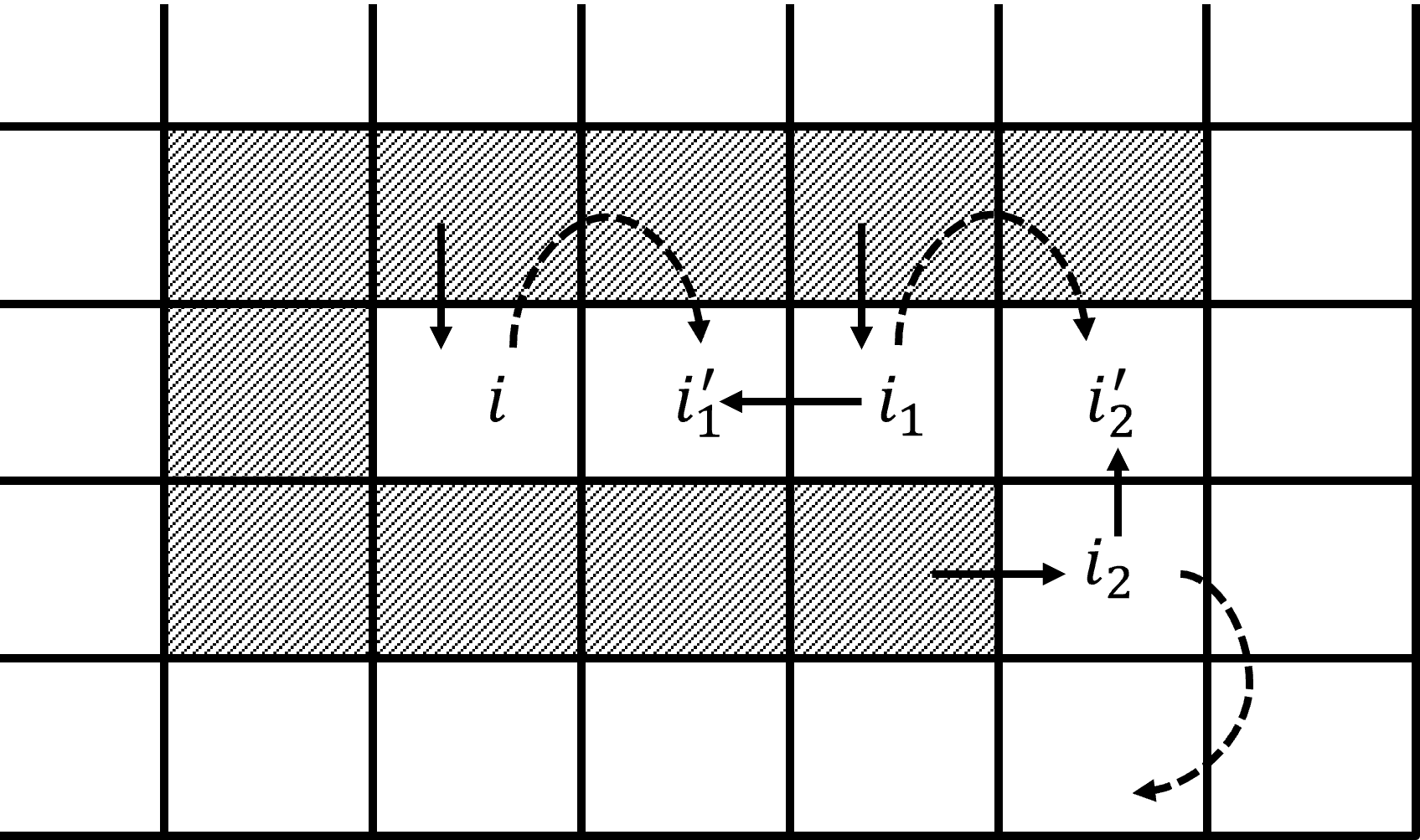
Figure 2: An example of movement adaption.

We propose in Algorithm 2 the pseudo-code for a movement-adaption method and provide in the following the explanations of the proposed steps. We refer to the policy resulted from Algorithm 2 as the movement-adapted index (MAI) policy. Let $a^{\rm MAI}_{i,i^{\prime},j}(\boldsymbol{s},t)$ ($i,i^{\prime}\in[I],j\in[J],t\in[T],\boldsymbol{s}\in\mathscr{S}$) represent the action variables of the MAI policy. For $i\in[I]$ and $j\in[J]$, let $d_{i,j}(\boldsymbol{s},\boldsymbol{\varpi})$ represent the distance from area $i$ to a vacant area given the state $\bm{S}^{\rm MAI}(t)=\boldsymbol{s}$ and $\boldsymbol{\varpi}\Bigl{(}\boldsymbol{a}^{\rm MAI}(\bm{S}^{\rm MAI}(t),t)\Bigr{)}=\boldsymbol{\varpi}$ with respect to agent-type $j$; more precisely, define

$$d_{i,j}(\boldsymbol{s},\boldsymbol{\varpi})=\left\{\begin{cases}0,&\text{if }\mathcal{i}(s_{i,j})=1,\text{ and }\exists i^{\prime}\in\mathscr{B}_{i,j}\text{ such that }\varpi_{i^{\prime},j}=0,\\ \min\nolimits_{\begin{subarray}{~{}}i^{\prime}\in\mathscr{B}_{i,j}:\\ \varpi_{i^{\prime},j}\neq i\end{subarray}}d_{\varpi_{i^{\prime},j}}+1,&\text{if }\mathcal{i}(s_{i,j})=1,\text{ and }\forall i^{\prime}\in\mathscr{B}_{i,j},~{}\varpi_{i^{\prime},j}>0,\\ \infty,&\text{otherwise}.\end{cases}\right.$$ (24)

Recall that we assume $|\mathscr{B}_{i,j}|\geq 2$ for all $(i,j)\in[I]\times[J]$. Hence, in the second case in (24), for each $(i,j)\in[I]\times[J]$, the set $\{i^{\prime}\in\mathscr{B}_{i,j}|\varpi_{i^{\prime},j}\neq i\}\neq\emptyset$.

We can initialize $d_{i,j}(\boldsymbol{s},\boldsymbol{\varpi})=\infty$ for all $(i,j)\in[I]\times[J]$. We find all the $(i,j)\in[I]\times[J]$ with $\mathcal{i}(s_{i,j})=1$ and existence of an $i^{\prime}\in\mathscr{B}_{i,j}$ such that $\varpi_{i^{\prime},j}=0$, and set $d_{i,j}(\boldsymbol{s},\boldsymbol{\varpi})=0$. Then iteratively obtain $d_{i^{\prime},j}(\boldsymbol{s},\boldsymbol{\varpi})$ for the direct neighbours $i^{\prime}\in\mathscr{B}_{i,j}$ of the area $i$ with previously determined $d_{i,j}(\boldsymbol{s},\boldsymbol{\varpi})<\infty$.

As presented in Algorithm 2, we initialize $\boldsymbol{a}^{\rm MAI}\bigl{(}\bm{S}^{\rm MAI}(t),t\bigr{)}$ with the value of the action vector $\boldsymbol{a}^{\rm IND}\bigl{(}\bm{S}^{\rm MAI}(t),t\bigr{)}$ by calling Algorithm 1 with $\bm{S}^{\rm IND}(t)$ substituted by $\bm{S}^{\rm MAI}(t)$. Based on the initialized $\boldsymbol{a}^{\rm MAI}\bigl{(}\bm{S}^{\rm MAI}(t),t\bigr{)}=\boldsymbol{a}$ and the given $\bm{S}^{\rm MAI}(t)=\boldsymbol{s}$, we can calculate the corresponding values of $\varpi_{i,j}(\boldsymbol{a})$ and $d_{i,j}(\boldsymbol{s},\boldsymbol{\varpi}(\boldsymbol{a}))$ for all $(i,j)\in[I]\times[J]$.

For each $j\in[J]$ and $i\in\mathscr{I}^{\rm MAI}_{j}(t)$, in Lines 2-2 of Algorithm 2, we find a path from the area $i$ to a vacant area through the movement adaption. In particular, we start with the area $i$ and replace a movement $(i^{*},\varpi,j)$ with $(i^{*},i,j)$, for which $\varpi=\varpi_{i^{*},j}\bigl{(}\boldsymbol{a}^{\rm MAI}(\boldsymbol{s},t)\bigr{)}$, $i^{*}$ is in $\mathscr{B}_{i,j}$, and the area $\varpi$ has the smallest distance to a vacant area (see Line 4). After this movement replacement, we find a place for the agent from area $i$ to stay in time slot $t$ while the agent in area $\varpi$ may have no place to go. Then we focus on $\varpi$ in the next while loop with appropriately updated variables. We will iteratively replace the selected movements until reaching a vacant area (that is, the stop condition in Line 2 is satisfied). The output action variables $\boldsymbol{a}^{\rm MAI}(\boldsymbol{s},t)$ form the MAI policy and satisfy Constraints (2). The MAI policy is applicable to the original patrol problem described in (3), (1) and (2).

In Section V-B, we prove that, under a mild condition related to the fine-tuned values of the cost rates, when the problem size grows to infinity, the index policy, the MAI policy and the optimality of the relaxed problem coincide with each other. Since MAI is applicable to the original problem, MAI also approaches optimality of the original problem.

1

2

Input : The state vector $\bm{S}^{\rm MAI}(t)=\boldsymbol{s}$ at time $t$.

Output : The action variables $a_{i,i^{\prime},j}^{\rm MAI}\bigl{(}\bm{S}^{\text{MAI}}(t),t\bigr{)}$ for $(i,i^{\prime},j)\in\bigcup_{j\in[J]}\mathscr{M}^{\text{MAI}}_{j}(t)$.

3

4Function MAIPolicy

       $a_{i,i^{\prime},j}^{\rm MAI}(\boldsymbol{s},t)\leftarrow a_{i,i^{\prime},j}^{\rm IND}(\boldsymbol{s},t)$ for $(i,i^{\prime},j)\in\bigcup_{j\in[J]}\mathscr{M}^{\text{MAI}}_{j}(t)$

        /* Initialize the action variables by calling Algorithm 1. */

5       Based on the action variables $a_{i,i^{\prime},j}^{\rm MAI}(\boldsymbol{s},t)$, initialize $\mathscr{I}^{\rm MAI}_{j}(t)$ for all $j\in[J]$, $\varpi_{i,j}\bigl{(}\boldsymbol{a}^{\rm MAI}(\boldsymbol{s},t)\bigr{)}$ for all $(i,j)\in[I]\times[J]$, and $d_{i,j}\Bigl{(}\boldsymbol{s},\boldsymbol{\varpi}\bigl{(}\boldsymbol{a}^{\rm MAI}(\boldsymbol{s},t)\bigr{)}\Bigr{)}$ described in (24) for all $(i,j)\in[I]\times[J]$.

6       $\varpi_{i,j}\leftarrow\varpi_{i,j}\bigl{(}\boldsymbol{a}^{\rm MAI}(\boldsymbol{s},t)\bigr{)}$ for all $(i,j)\in[I]\times[J]$

7       $d_{i,j}\leftarrow d_{i,j}\Bigl{(}\boldsymbol{s},\boldsymbol{\varpi}\bigl{(}\boldsymbol{a}^{\rm MAI}(\boldsymbol{s},t)\bigr{)}\Bigr{)}$ for all $(i,j)\in[I]\times[J]$

8       for $j=1,2,\ldots,J$ do

9             for $\forall i\in\mathscr{I}^{\rm MAI}_{j}(t)$ do

10                   $\bar{i}\leftarrow i$

11                   while $\bar{i}>0$ do

12                         $i^{*}\leftarrow\min\arg\min_{i^{\prime}\in\mathscr{B}_{\bar{i},j}}d_{\varpi_{i^{\prime},j},j}$

13                         $\varpi\leftarrow\varpi_{i^{*},j}$

14                         $a^{\rm MAI}_{i^{*},\bar{i},j}(\boldsymbol{s},t)\leftarrow 1$

                         $a^{\rm MAI}_{i^{*},\varpi,j}(\boldsymbol{s},t)\leftarrow 0$

                          /* Replace movement $(i^{*},\varpi,j)$ with $(i^{*},\bar{i},j)$ */

15                         if $d_{\varpi,j}=0$ then

16                               Find an $i^{\prime}\in\mathscr{B}_{\varpi,j}$ such that $\varpi_{i^{\prime},j}=\infty$

                               $a^{\rm MAI}_{i^{\prime},\varpi,j}(\boldsymbol{s},t)\leftarrow 1$

                                /* Take the movement $(i^{\prime},\varpi,j)$ */

17                               $\varpi_{i^{\prime},j}\leftarrow\varpi$

18                               $\varpi_{i^{*},j}\leftarrow\bar{i}$

19                               $\bar{i}\leftarrow 0$

20                              

21                         end if

22                        else

23                               Exchange the values of variables $\varpi_{i^{*},j}$ and $\bar{i}$

24                              

25                         end if

26                        

27                   end while

28                  Based on the updated $\boldsymbol{\varpi}\coloneqq(\varpi_{i,j}:i\in[I],j\in[J])$, update the values of $d_{i^{\prime},j}(\boldsymbol{s},\boldsymbol{\varpi})$ for all $i^{\prime}\in[I]$ that satisfy (24).

29                   $d_{i^{\prime},j}\leftarrow d_{i^{\prime}j}(\boldsymbol{s},\boldsymbol{\varpi})$ for all $i^{\prime}\in[I]$

30                  

31             end for

32            

33       end for

34      return $a_{i,i^{\prime},j}^{\rm MAI}\bigl{(}\bm{S}^{\text{MAI}}(t),t\bigr{)}$ for $(i,i^{\prime},j)\in\bigcup_{j\in[J]}\mathscr{M}^{\text{MAI}}_{j}(t)$

35      

36 End

Algorithm 2 Pseudo-code for the movement adaption.

IV-B Computational Complexity of MAI

Recall that, as described in Section IV-A, MAI is based on the indices defined in (22). The values of the indices $\eta_{i,i^{\prime},j}(s,t)$ for all $i,i^{\prime}\in[I]$, $j\in[J]$, $s\in\mathscr{S}_{i,j}$, and $t\in[T]$ are computed a priori in an offline manner. From the definition in (22), the indices are in closed forms when the optimal solution $\boldsymbol{\gamma}^{*}$ and $\bm{V}^{*}$ of the dual problem described in (16)-(17) are given. Recall that the dual problem in (16)-(17) is a linear programming problem with $N=(T+1)\sum\nolimits_{(i,j)\in[I]\times[J]}|\mathscr{S}_{i,j}|+IJT$ variables and $2T\sum\nolimits_{(i,j)\in[I]\times[J]}|\mathscr{S}_{i,j}|=\Omega(N)$ constraints. It can be solved through conventional linear programming methods, such as the interior point methods [29, 30] with complexity no worse than $O(N^{2.5})$.

With given indices, the computational complexity for MAI consists of three cascading parts: ranking the movements based on the pre-computed indices $\bm{\eta}$ (described in (22)), determining the actions for the index policy with the ranked movements (pseudo-code in Algorithm 1), and the movement adaption process (pseudo-code in Algorithm 2). All the three parts are processed online with observed system state $\bm{S}^{\text{MAI}}(t)$ at time $t$. As described in Definition Movement Ranking, we rank the movements for each $j\in[J]$ according to the pre-computed $\bm{\eta}$ and the states $S^{\text{MAI}}_{i,j}(t)$ ($(i,j)\in[I]\times[J]$) at time $t$. For $\phi\in\Phi$ and $t$, define $\Psi^{\phi}(t)\coloneqq\sum_{j\in[J]}|\mathscr{M}^{\phi}_{j}(t)|$. At a time slot $t\in[T]$, for each $j\in[J]$, the computational complexity to maintain the set $\mathscr{M}^{\text{MAI}}_{j}(t)$ and rank the $|\mathscr{M}^{\text{MAI}}_{j}(t)|$ movements is no worse than $O(\Psi^{\text{MAI}}(t))$ and $O(\Psi^{\text{MAI}}(t)\log\Psi^{\text{MAI}}(t))$, respectively. The index policy can be constructed through the steps in Algorithm 1, for which the computational complexity is $O(\Psi^{\text{MAI}}(t))$. Taking $B\coloneqq\max_{i,j}|\mathscr{B}_{i,j}|$, we obtain that $\Psi^{\text{MAI}}(t)\leq\sum_{j\in[J]}M_{j}B$ for any $t\in[T]$. Hence, the total computational complexity for the first two parts is $O(\sum_{j\in[J]}M_{j}B\log(\sum_{j\in[J]}M_{j}B))$.

The third part, movement adaption, is processed through Algorithm 2, which includes initialization steps and three levels of loops. The computational complexity of the initialization steps is no worse than $O(IJB+\sum\nolimits_{j\in[J]}M_{j}B)$. The external loop with variable $j\in[J]$ iterates $J$ times. The second-level loop with variable $i\in\mathscr{I}^{\text{MAI}}_{j}(t)$ repeats $O(I)$ times. The internal loop from Line 2 to 2 iterates at most $d_{\bar{i},j}=O(I)$ times, each of which has complexity $O(B)$ mainly incurred by the minimum operation in Line 2. In Line 2, updating the area distances for each $j\in[J]$ costs $O(IB+M_{j}B)$. Since $M_{j}\leq I$, the worst case complexity is $O(IB)$. Hence, the overall computational complexity of Algorithm 2 is at most $O(I^{2}JB)$.

For each time slot $t$, the computational complexity for implementing MAI (the above-mentioned three cascading parts) is $O\bigl{(}MB\log(MB)+I^{2}JB\bigr{)}$, where $M=\sum_{j\in[J]}M_{j}$ representing the total number of agents, and $I$ and $J$ are the numbers of different areas and agent types, respectively.

V Asymptotic Optimality

V-A Asymptotic Regime

Consider a large number $h\in\mathbb{N}_{+}$ of highly sophisticated sensors that are used to precisely explore tiny sub-areas located in the geographical region. In particular, we divide each area $i\in[I]$ into $h$ sub-areas, referred to as the sub-areas $(i,k)$ ($i\in[I]$, $k\in[h]$), each of which is related to $J$ stochastic processes $\{S^{\phi,k}_{i,j}(t),t\in[T]\}$ ($j\in[J]$) with state space $\mathscr{S}_{i,j}$. The transition probabilities of the process $\{S^{\phi,k}_{i,j}(t):t\in[T]\}$ are the same as $\{S^{\phi}_{i,j}(t):t\in[T]\}$ defined in Section II. The number of agents of type $j\in[J]$ is considered to be $M_{j}=hM_{j}^{0}$ for some $M_{j}^{0}\in\mathbb{N}_{+}$. Within a unit time, an agent in the sub-area $(i,k)$ ($i\in[I]$, $k\in[h]$) can move to any sub-area in the neighbourhood of the area $i$ (that is, the agent can move to any sub-area $(i^{\prime},k^{\prime})$ with $i^{\prime}\in\mathscr{B}_{i,j}$ and $k^{\prime}\in[h]$). We refer to $h$ as the scaling parameter of the patrol system and refer to the system with the scaling parameter as the system scaled by $h$. As $h$ increases, the patrol region is divided into increasingly many sub-areas explored by compatible numbers of different agents. More sub-areas and agents indicate larger geographical region or the same region with higher precision of collected information and more careful exploration. The patrol system defined and discussed in the above sections is a special case of the scaled system with $h=1$.

Let $\bm{S}^{\phi,h}(t)\coloneqq(S^{\phi,k}_{i,j}(t):i\in[I],j\in[j],k\in[h])$. For $i,i^{\prime}\in[I]$, $j\in[J]$, $k\in[h]$, $\boldsymbol{s}\in\mathscr{S}$, and $t\in[T]$, define action variables $a^{\phi,k}_{i,i^{\prime},j}(\boldsymbol{s},t)$ associated with the policy $\phi$ and taking binary values: if $a^{\phi,k}_{i,i^{\prime},j}(\boldsymbol{s},t)=1$ then, when $\bm{S}^{\phi}(t)=\boldsymbol{s}$, an agent of type $j$ moves from a sub-area of area $i^{\prime}$ to sub-area $(i,k)$ at the beginning of time slot $t$ and explores there before the next time slot; otherwise, no such a movement. If $i^{\prime}\in[I]\backslash\mathscr{B}_{i,j}$, then $a^{\phi,k}_{i,i^{\prime},j}(\boldsymbol{s},t)\equiv 0$. In a scaled system, let $\Phi^{h}$ represent the set of all the policies determined by such action variables, and, for $i,j\in[I]\times[J]$, $k\in[h]$, $\boldsymbol{s}\in\mathscr{S}$, $\phi\in\Phi^{h}$ and $t\in[T]$, let $\boldsymbol{a}^{\phi,k}_{i,j}(\boldsymbol{s},t)\coloneqq(a^{\phi,k}_{i,i^{\prime},j}(\boldsymbol{s},t):i^{\prime}\in[I])$. We generalize the problem in (3), (1) and (2) to its scaled version,

$$\min\limits_{\phi\in\Phi^{h}}\frac{1}{h}\sum\limits_{t\in[T]}\sum\limits_{i\in[I]}\sum\limits_{j\in[J]}\sum\limits_{k\in[h]}\mathbb{E}\Bigl{[}c_{i,j}\Bigl{(}S^{\phi,k}_{i,j}(t),\mathcal{e}^{\phi,k}_{i,j}\bigl{(}\bm{S}^{\phi,h}(t),t\bigr{)},t\Bigr{)}\Bigr{]},$$ (25)

where $\mathcal{e}^{\phi,k}_{i,j}(\bm{S}^{\phi,h}(t),t)\coloneqq\mathds{1}\bigl{\{}\sum_{i^{\prime}\in\mathscr{B}_{i,j}}a^{\phi,k}_{i,i^{\prime},j}\bigl{(}\bm{S}^{\phi}(t),t\bigr{)}>0\bigr{\}}$, subject to

$$\frac{1}{h}\sum\limits_{i^{\prime}\in\mathscr{B}_{i,j}}\sum\limits_{k\in[h]}a^{\phi,k}_{i,i^{\prime},j}\Bigl{(}\bm{S}^{\phi,h}(t),t\Bigr{)}\leq 1,~{}\forall i\in[I],j\in[J],t\in[T],$$ (26)

and

$$\frac{1}{h}\sum\limits_{i^{\prime}\in\mathscr{B}_{i,j}}\sum\limits_{k\in[h]}a^{\phi,k}_{i^{\prime},i,j}\bigl{(}\bm{S}^{\phi,h}(t),t\bigr{)}=\frac{1}{h}\sum\limits_{k\in[h]}I^{\phi,k}_{i,j}(t),~{}\forall i\in[I],j\in[J],t\in[T].$$ (27)

The $1/h$ in (25), (26) and (27) is used to make all the expressions finite when $h\rightarrow+\infty$. Constraints (26) guarantee that there are at most $h$ sub-areas in each area $i$ that can be explored by agents of each type $j$ at each time slot, where each sub-area is explored by at most one agent of the the same type at the same time slot. Based on Constraints (27), each agent must move to its neighbourhood, including staying in its current location, within a unit time. The problem described in (3), (1) and (2) is a special case of the above problem by setting $h=1$. We refer to the problem described in (25), (26) and (27) as the scaled patrol problem. We refer to the case with $h\rightarrow+\infty$ as the asymptotic regime.

Similar to the special case in Section III, we randomize the action variables $a^{\phi,k}_{i,i^{\prime},j}(\boldsymbol{s},t)$ and relax (27) to

$$\frac{1}{h}\sum\limits_{i^{\prime}\in\mathscr{B}_{i,j}}\sum\limits_{k\in[h]}\alpha^{\phi,k}_{i^{\prime},i,j}\bigl{(}S^{\phi,k}_{i^{\prime},j}(t),t\bigr{)}=\frac{1}{h}\sum\limits_{k\in[h]}\mathbb{E}\Bigl{[}I^{\phi,k}_{i,j}(t)\Bigr{]},~{}\forall i\in[I],j\in[J],t\in[T],$$ (28)

where $\alpha^{\phi,k}_{i,i^{\prime},j}(s,t)\coloneqq\mathbb{E}\bigl{[}a^{\phi,k}_{i,i^{\prime},j}\bigl{(}\bm{S}^{\phi,h}(t),t\bigr{)}|S^{\phi,k}_{i,j}(t)=s\bigr{]}$, representing the probability of taking $a^{\phi,k}_{i,i^{\prime},j}\bigl{(}\bm{S}^{\phi,h}(t),t\bigr{)}=1$ when $S^{\phi,k}_{i,j}(t)=s$. Define $\tilde{\Phi}^{h}$ as the set of all the policies $\phi$ determined by such action variables $\alpha^{\phi,k}_{i,i^{\prime},j}(s,t)$ for all $i,i^{\prime}\in[I]$, $j\in[J]$, $k\in[h]$, $t\in[T]$ and $s\in\mathscr{S}_{i,j}$ with satisfied (26). We refer to the problem

$$\min\limits_{\phi\in\tilde{\Phi}^{h}}\frac{1}{h}\sum\limits_{t\in[T]}\sum\limits_{i\in[I]}\sum\limits_{j\in[J]}\sum\limits_{k\in[h]}\mathbb{E}\Bigl{[}c_{i,j}\Bigl{(}S^{\phi,k}_{i,j}(t),\mathcal{e}^{\phi,k}_{i,j}\bigl{(}\bm{S}^{\phi,k}_{i,j},t\bigr{)},t),t\Bigr{)}\Bigr{]},$$ (29)

subject to (28) as the relaxed version of the problem in the scaled system. Recall that the $1/h$ in (29) is used to keep the minimum finite when $h\rightarrow+\infty$.

The relaxed problem in the scaled system can be decomposed along the same lines as described in Section III, resulting in $IJh$ sub-problems that are associated with the $IJh$ sub-processes $\Bigl{\{}S^{\phi,k}_{i,j}(t),t\in[T]\Bigr{\}}$ ($i\in[I]$, $j\in[J]$ and $k\in[h]$). We still use $\boldsymbol{\gamma}\in\mathbb{R}^{IJT}$ to represent the Lagrange multipliers for (28). More precisely, for $i\in[I]$, $j\in[J]$, $k\in[h]$, $\phi\in\tilde{\Phi}^{h}$, and $\boldsymbol{\gamma}_{i,j}\in\mathbb{R}^{T}$, define

$$L^{\phi,k}_{i,j}(\boldsymbol{\gamma}_{i,j})\coloneqq\sum\limits_{t\in[T]}\sum\limits_{s\in\mathscr{S}_{i,j}}\sum\limits_{\boldsymbol{a}\in\mathscr{A}_{i,j}}C^{\boldsymbol{\gamma}_{i,j}}_{i,j}(s,\boldsymbol{\alpha}^{\phi,k}_{i,j}\bigl{(}s,t\bigr{)},t)\mathbb{P}\Bigl{[}S^{\phi,k}_{i,j}(t)=s\Bigr{]},$$ (30)

and the dual function of the relaxed problem in (29) and (28) is

$$L^{h}(\boldsymbol{\gamma})=\frac{1}{h}\min\limits_{\phi\in\tilde{\Phi}^{h}}\sum\limits_{i\in[I]}\sum\limits_{j\in[J]}\sum\limits_{k\in[h]}L^{\phi,k}_{i,j}(\boldsymbol{\gamma}_{i,j})=\sum\limits_{i\in[I]}\sum\limits_{j\in[J]}\sum\limits_{k\in[h]}\min\limits_{\phi_{i,j}\in\tilde{\Phi}^{h}}L^{\phi_{i,j},k}_{i,j}(\boldsymbol{\gamma}_{i,j}),$$ (31)

where $\boldsymbol{\gamma}$ are the Lagrange multipliers, $\boldsymbol{\gamma}_{i,j}=(\gamma_{i,j,t}:t\in[T])$, and the second equality is a direct result of Proposition 1. Similar to the special case in Section III, we refer to $\min_{\phi_{i,j}\in\tilde{\Phi}^{h}}L^{\phi_{i,j},k}_{i,j}(\boldsymbol{\gamma}_{i,j})$ as the sub-problem of the sub-AA pair $(i,j,k)\in[I]\times[J]\times[h]$. Given $(i,j)\in[I]\times[J]$, the sub-AA pairs $(i,j,k)$ lead to the same sub-problem for any $k\in[h]$.

It follows that the linear problem in (16)-(18) achieves the same minimum as the dual problem of the relaxed problem in the scaled system upon the same solution $\boldsymbol{\gamma}^{*}$ and $\bm{V}^{*}$. For $(i,j)\in[I]\times[J]$ and any $k\in[h]$, Lemma 1 and Proposition 2 can be directly applied to the sub-problems in the scaled system with added superscript $k$ to the variables $\boldsymbol{\alpha}^{\phi}_{i,j}(\cdot,\cdot)$, $S^{\phi}_{i,j}(t)$ and $L^{\phi}_{i,j}(\boldsymbol{\gamma}_{i,j})$. The index and MAI policy can be applied along similar lines as those described in Section IV-A. In Appendix G, we also provide the pseudo-codes for the index and the MAI policy in the scaled system. The computational complexity of the MAI policy can be analysed through the same steps, but is scaled by the parameter $h$ compared to the special case discussed in Section IV-B. It follows with complexity $O(MB\log(MB)+I^{2}JBh\bar{M})$, where $M=\sum\nolimits_{j\in[J]}M^{0}_{j}h$ is the total number of agents in the scaled system, and $\bar{M}\in[h]$ is the maximal number of agents in a single area that have no place to be located at a time slot under the index policy. Based on the discussion in Appendix E, the difference between MAI and the index policy becomes negligible as $h$ approaches infinity, and $\bar{M}=o(h)$.

V-B Asymptotic Optimality

We extend the techniques of [21, 36, 24] to the case discussed in this paper and prove asymptotic optimality of the index policy proposed in (23). We prove in Theorem 3 that the MAI policy coincides with the index policy (described in (23)) and approaches optimality of the relaxed problem as $h\rightarrow+\infty$ under a provided condition. This condition is related to the trajectory of the stochastic process of the entire system and is similar to the conventional request of a global attractor for the standard RMAB process. We further prove that, when each area is strictly indexable, this condition is satisfied, and then the MAI policy approaches optimality in the asymptotic regime. Since the MAI policy is applicable to the original problem, it also approaches optimality of the original problem as $h\rightarrow+\infty$. That is, with strictly indexable areas, the MAI policy is asymtpotically optimal.

Consider an integer $M\in\mathbb{N}_{+}$, policies $\phi^{*}_{1},\phi^{*}_{2},\ldots,\phi^{*}_{M}\in\tilde{\Phi}^{h}$ such that satisfy (19) for all $(i,j,k)\in[I]\times[J]\times[h]$ with $\boldsymbol{\gamma}_{i,j}$ and $\phi_{i,j}(\boldsymbol{\gamma}^{*}_{i,j})$ replaced by $\boldsymbol{\gamma}^{*}_{i,j}$ and $\phi^{*}_{m}$ ($m\in[M]$), respectively, and a probability vector $\bm{\pi}^{*}\in[0,1]^{M}$ as such that (21) is satisfied together with these $\phi^{*}_{m}$ ($m\in[M]$). The existence of such $M$, $\phi^{*}_{m}$, and $\pi^{*}_{m}$ is guaranteed by Proposition 2. Let $\bm{\phi}^{*}\coloneqq(\phi^{*}_{m}:m\in[M])$. Define a mixed policy $\psi(M,\bm{\phi}^{*},\bm{\pi}^{*})$ by mixing these policies $\phi^{*}_{1},\phi^{*}_{2},\ldots,\phi^{*}_{M}$. More precisely, we say an mixed policy $\psi(M,\bm{\phi}^{*},\bm{\pi}^{*})$ is employed if, for each AA-pair $(i,j)\in[I]\times[J]$ and $m\in[M-1]$, $\lfloor\pi^{*}_{m}h\rfloor$ of the sub-processes associated with the AA-pair $(i,j)$ are under the policy $\phi^{*}_{m}$, and the remaining $h-\sum_{m\in[M-1]}\lfloor\pi_{m}h\rfloor$ sub-processes follow the policy $\phi^{*}_{M}$. Let $k^{-}(m)\coloneqq\sum_{m^{\prime}\in[m]}\lfloor\pi^{*}_{m^{\prime}}h\rfloor$ for $m\in[M-1]$, $k^{-}(0)=0$ and $k^{-}(M)=h$. Without loss of generality, for the policy $\psi(M,\bm{\phi}^{*})$, we assume that, for each $(i,j)\in[I]\times[J]$ and $m\in[M]$, sub-processes $(i,j,k)$ with $k=k^{-}(m-1)+1,k^{-}(m-1)+2,\ldots,k^{-}(m)$ are under the policy $\phi^{*}_{m}$. The mixed policy $\psi(M,\bm{\phi}^{*},\bm{\pi}^{*})$, abbreviated as $\psi^{*}$, satisfies (26) but not necessarily comply with (28). It is not necessarily applicable to the relaxed problem. It will be used to establish a relationship between a policy applicable to the original problem (that is, a policy $\phi\in\Phi^{h}$ satisfying (26)) and an optimal solution to the relaxed problem.

For $\phi\in\tilde{\Phi}^{h}$ and $h\in\mathbb{N}_{+}$, define

$$\Gamma^{h,\phi}\coloneqq\frac{1}{h}\sum\limits_{t\in[T]}\sum\limits_{t\in[I]}\sum\limits_{j\in[J]}\sum\limits_{k\in[h]}\mathbb{E}\Bigl{[}c_{i,j}\Bigl{(}S^{\phi,k}_{i,j}(t),\mathcal{e}^{\phi,k}_{i,j}\bigl{(}\bm{S}^{\phi,h}(t),t\bigr{)},t\Bigr{)}\Bigr{]},$$ (32)

as the expected cumulative cost of process $\{\bm{S}^{\phi,h}(t):~{}t\in[T]\}$ under policy $\phi$. Let $\hat{\Phi}^{h}\subset\tilde{\Phi}^{h}$ represent the set of all policies in $\tilde{\Phi}^{h}$ complying Constraints  (28) (applicable to the relaxed problem), and define $\Gamma^{h,*}\coloneqq\min_{\phi\in\hat{\Phi}^{h}}\Gamma^{h,\phi}$ represent the mminimum of the relaxed problem described by (29) and (28).

Theorem 3 (Asymptotic Optimality)

For a policy $\phi\in\Phi^{h}$ satisfying (27), if, for all $t\in[T]$,

$$\lim\limits_{h\rightarrow+\infty}\bigl{\lvert}\Gamma^{h,\phi}-\Gamma^{h,\psi^{*}}\bigr{\rvert}=0,$$ (33)

then

$$\lim\limits_{h\rightarrow+\infty}\bigl{\lvert}\Gamma^{h,\phi}-\Gamma^{h,*}\bigr{\rvert}=0.$$ (34)

The proof of Theorem 3 is provided in Appendix D. A policy $\phi\in\Phi^{h}$ satisfying (27) is in fact applicable to the original problem described in (25) and (27). For such a policy $\phi$ applicable to the original problem, since $\phi\in\hat{\Phi}^{h}$ and $\Gamma^{h,*}$ is a lower bound of minimum of the original problem, Theorem 3 indicates that $\phi$ approaches optimality of the original problem as $h\rightarrow+\infty$; that is, such a policy $\phi$ is asymptotically optimal to the original problem.

Proposition 4

If all the areas are strictly indexable, then the MAI policy satisfies (33) by setting $\phi=$MAI, and MAI is asymptotically optimal.

The proof of Proposition 4 is provided in Appendix E. Proposition 4 is based on Theorem 3 and ensures a lower bound for the performance of MAI. More importantly, we achieve the following theorem that bounds the performance deviation between the MAI policy and an optimal solution of the original problem for a finite $h<+\infty$.

Theorem 5 (Exponential Convergence)

If all the areas are strictly indexable, then, for any $\delta>0$, there exists $H>0$ and $s>0$ such that, for all $h>H$,

$$\bigl{\lvert}\Gamma^{h,\rm MAI}-\Gamma^{h,*}\bigr{\rvert}\leq e^{-sh}+\delta.$$ (35)

The theorem is proved in Appendix F. In (35), $\delta$ is a precision parameter that can be arbitrarily small. Theorem 5 ensures that the performance deviation between the MAI policy and an optimal solution of the original problem diminishes exponentially in the scaling parameter $h$. It implies that the MAI policy becomes sufficiently close to optimality even in a relatively small system and will be better when the problem size keeps increasing.

The strict indexability (Definition Indexability) for all areas can be achieved by appropriately attaching a sufficiently small $\epsilon_{i,j}(s,a,t)>0$ to the cost rate $c_{i,j}(s,a,t)$ ($(i,j)\in[I]\times[J]$, $s\in\mathscr{S}_{i,j}$, $a\in\{0,1\}$ and $t\in[T]$). Compare to the absolute value of $\Gamma^{h,*}$, such $\epsilon_{i,j}(s,a,t)>0$ ($(i,j)\in[I]\times[J]$, $s\in\mathscr{S}_{i,j}$, $a\in\{0,1\}$ and $t\in[T]$) are designed to be negligible, while they are crucial to determine the ranking of all the MASTs $\iota\in[N]$ with achieved strict indexability.

Note that the asymptotically optimal patrol policy is not necessarily unique. We have proved in Theorem 3 that any policy satisfying (33) is asymptotically optimal. In particular, the MAI policy described in Section IV can be implemented through various ways of adapting the movements. Different movement-adaption methods potentially lead to different action variables; more rigorously, different policies. Although MAI with different movement-adaption methods potentially lead to different performances in the non-asymptotic regime, from Theorem 5, MAI will quickly converge to an optimal solution and will be already close to optimality in the non-asymptotic regime.

VI Conclusions

We have model the patrolling problem as a set of discrete-time bandit processes that extend the assumptions on the past patrolling models, such as identical agents, submodular reward functions and capability of sensing any location at any time. We have captured the relationship between the eligible movements, positions and profiles of the agents through Constraints (1) and (2), leading to a stronger dependency among the action and state variables of the bandit processes than that of the conventional RMAB problem. The patrolling problem is complicated by the high dimension of its state space that increases at least exponentially in the number of agents and the size of the patrolling region. The past RMAB methods cannot ensure the existence of scalable patrol policies with theoretically bounded performance degradation.

We have extended the Whittle relaxation and Lagranian DP techniques to the patrolling problem to decompose the state space exhibiting curse of dimensionality. We have proposed the MAI policy with computational complexity $O(MB\log(MB)+I^{2}JBh\bar{M})$, where $\bar{M}=o(h)$, for a system with scaling parameter $h$. Recall that increasing $h$ indicates larger geographical patrol region or the same region with higher precision of collected information and more careful exploration. In Theorem 3, we have provided a sufficient and necessary condition for asymptotic optimality. Based on Theorem 3 and Proposition 4, we have proved that, when the areas are strictly indexably, the MAI policy approaches optimality as $h\rightarrow+\infty$. More importantly, from Theorem 5, we have proved that, with strictly indexable areas, the performance deviation between MAI and optimality diminishes exponentially as $h$ increases.

Appendix A Proof of Proposition 1

Proof of Proposition 1.  Consider the sum of minimum

$$\sum\limits_{i\in[I]}\sum\limits_{j\in[J]}\min\limits_{\phi_{i,j}\in\tilde{\Phi}}L^{\phi_{i,j}}_{i,j}(\boldsymbol{\gamma}_{i,j})\leq\min\limits_{\phi\in\tilde{\Phi}}\sum\limits_{i\in[I]}\sum\limits_{j\in[J]}L^{\phi}_{i,j}(\boldsymbol{\gamma}_{i,j})=L(\boldsymbol{\gamma}).$$ (36)

The inequality comes from the concavity of minimization operation. For each of the minimum associated with the AA pair $(i,j)$ at the left hand side of (36),

$$\min\limits_{\phi_{i,j}\in\tilde{\Phi}}L^{\phi_{i,j}}_{i,j}(\boldsymbol{\gamma}_{i,j})=\sum\limits_{\boldsymbol{s}\in\mathscr{S}}\pi^{0}(\boldsymbol{s})V^{\boldsymbol{\gamma}_{i,j}}_{i,j}(\boldsymbol{s},1),$$ (37)

where $\pi^{0}(\boldsymbol{s})$ is the given probability of the initial state $\bm{S}^{\phi}(1)=\boldsymbol{s}$, and $V^{\boldsymbol{\gamma}_{i,j}}_{i,j}(\boldsymbol{s},t)$ ($i\in[I]$, $j\in[J]$, $t\in[T]$, $\boldsymbol{s}\in\mathscr{S}$) is the minimal expected cumulative cost from time $t$ to $T$ given the state $\bm{S}^{\phi}(t)=\boldsymbol{s}$ at time $t$ of the sub-process $(i,j)$. Recall that a policy $\phi_{i,j}\in\tilde{\Phi}$ is determined by its action variables $\bar{a}^{\phi_{i,j}}_{i,i^{\prime},j}(\boldsymbol{s},t)$ ($i,i^{\prime}\in[I]$,$j\in[J]$, $t\in[T]$, $\boldsymbol{s}\in\mathscr{S}$). Consider the Bellman equation for the sub-process $(i,j)\in[I]\times[J]$.

$$V^{\boldsymbol{\gamma}_{i,j}}_{i,j}(\boldsymbol{s},t)=\min\limits_{\phi\in\tilde{\Phi}}\Bigl{\{}C^{\boldsymbol{\gamma}_{i,j}}_{i,j}(s_{i,j},\bar{\boldsymbol{a}}^{\phi}_{i,j}(\boldsymbol{s},t),t)+\sum\limits_{\boldsymbol{s}^{\prime}\in\mathscr{S}}P_{t}(\boldsymbol{s},\bar{\boldsymbol{a}}^{\phi}(\boldsymbol{s},t),\boldsymbol{s}^{\prime})V^{\boldsymbol{\gamma}_{i,j}}_{i,j}(\boldsymbol{s}^{\prime},t+1)\Bigr{\}},$$ (38)

with $V^{\boldsymbol{\gamma}_{i,j}}_{i,j}(\boldsymbol{s},T+1)\equiv 0$ for all $\boldsymbol{s}\in\mathscr{S}$, where $\bar{\boldsymbol{a}}^{\phi}(\boldsymbol{s},t)\coloneqq(\bar{a}^{\phi}_{i,i^{\prime},j}(\boldsymbol{s},t):i,i^{\prime}\in[I],j\in[J])$, and $P_{t}(\boldsymbol{s},\boldsymbol{a},\boldsymbol{s}^{\prime})$ is the transition probability from $\boldsymbol{s}$ to $\boldsymbol{s}^{\prime}$ after action $\boldsymbol{a}$ is taken.

For $i\in[I]$, $j\in[J]$, and given $s\in\mathscr{S}_{i,j}$, if $\bar{\boldsymbol{a}}^{\phi}_{i,j}(\boldsymbol{s},T)=\boldsymbol{a}$ ($\boldsymbol{a}\in\mathscr{A}_{i,j}$) minimizes the right hand side of (38), then there exists an optimal policy $\phi_{i,j}\in\tilde{\Phi}$ for $\min_{\phi\in\tilde{\Phi}}L^{\phi}_{i,j}(\boldsymbol{\gamma}_{i,j})$ such that, for any $\boldsymbol{s}^{\prime}\in\mathscr{S}$ with $s^{\prime}_{i,j}=s_{i,j}$, $\bar{\boldsymbol{a}}^{\phi_{i,j}}_{i,j}(\boldsymbol{s}^{\prime},T)=\boldsymbol{a}$. That is, $\bar{\boldsymbol{a}}^{\phi_{i,j}}_{i,j}(\boldsymbol{s},T)$ and $V^{\boldsymbol{\gamma}_{i,j}}_{i,j}(\boldsymbol{s},T)$ dependent on $\boldsymbol{s}$ through only $s_{i,j}$. For any $t\in[T-1]$, assume that there exists an optimal policy $\phi_{i,j}\in\tilde{\Phi}$ for $\min\limits_{\phi\in\tilde{\Phi}}L^{\phi}_{i,j}(\boldsymbol{\gamma}_{i,j})$ where, for $\tau=t+1,t+2\ldots,T$ and any $\boldsymbol{s}^{\prime}\in\mathscr{S}$, $\bar{\boldsymbol{a}}^{\phi_{i,j}}_{i,j}(\boldsymbol{s},\tau)$ and $V^{\boldsymbol{\gamma}_{i,j}}_{i,j}(\boldsymbol{s},\tau)$ are dependent on $\boldsymbol{s}$ through only $s_{i,j}$. In this context, given $s_{i,j}\in\mathscr{S}_{i,j}$, if $\bar{\boldsymbol{a}}^{\phi}_{i,j}(\boldsymbol{s},t)=\boldsymbol{a}$ ($\boldsymbol{a}\in\mathscr{A}_{i,j}$) minimizes the right hand side of (38) for some $\boldsymbol{s}\in\mathscr{S}$, then, for any $\boldsymbol{s}^{\prime}\in\mathscr{S}$ with $s^{\prime}_{i,j}=s_{i,j}$, there exists an optimal policy $\phi_{i,j}$ such that $\bar{\boldsymbol{a}}^{\phi_{i,j}}_{i,j}(\boldsymbol{s},t)=\boldsymbol{a}$. Hence, for any $i\in[I]$, $j\in[J]$, $t\in[T]$ and $\boldsymbol{s}\in\mathscr{S}$, there exists an optimal policy $\phi_{i,j}\in\tilde{\Phi}$ for $\min\limits_{\phi\in\tilde{\Phi}}L^{\phi}_{i,j}(\boldsymbol{\gamma}_{i,j})$ such that $\bar{\boldsymbol{a}}^{\phi_{i,j}}_{i,j}(\boldsymbol{s},t)$ and $V^{\boldsymbol{\gamma}_{i,j}}_{i,j}(\boldsymbol{s},t)$ are dependent on $\boldsymbol{s}$ through only $s_{i,j}$. We rewrite $V^{\boldsymbol{\gamma}_{i,j}}_{i,j}(\boldsymbol{s},t)$ as $V^{\boldsymbol{\gamma}_{i,j}}_{i,j}(s_{i,j},t)$ and obtain

$$V^{\boldsymbol{\gamma}_{i,j}}_{i,j}(\boldsymbol{s},t)=V^{\boldsymbol{\gamma}_{i,j}}_{i,j}(s_{i,j},t)=\min\limits_{\boldsymbol{a}\in\mathscr{A}_{i,j}}\Bigl{\{}C^{\boldsymbol{\gamma}_{i,j}}_{i,j}(s_{i,j},\boldsymbol{a},t)+\sum\limits_{s^{\prime}_{i,j}\in\mathscr{S}_{i,j}}P_{i,j,t}(s_{i,j},\mathcal{e}(\boldsymbol{a}),s^{\prime}_{i,j})V^{\boldsymbol{\gamma}_{i,j}}_{i,j}(s^{\prime}_{i,j},t+1)\Bigr{\}},$$ (39)

where recall that, for $\boldsymbol{a}=(a_{i^{\prime}}:i^{\prime}\in[I])\in\mathscr{A}_{i,j}$, $\mathcal{e}_{i,j}(\boldsymbol{a})=1-\prod_{i^{\prime}\in[I]}(1-a_{i^{\prime}})$ representing the probability of moving a type-$j$ agent to the area $i$ under the action $\boldsymbol{a}$, and $P_{i,j,t}(s_{i,j},\mathcal{e}(\boldsymbol{a}),s^{\prime}_{i,j})$ is the transition probability from state $s_{i,j}$ to $s^{\prime}_{i,j}$. We can solve (39) for all $(i,j)\in[I]\times[J]$ independently. Construct a policy $\phi\in\bar{\Phi}$ consisting of the optimal actions that minimize the right hand side of (39) for all $(i,j)\in[I]\times[J]$, $t\in[T]$ and $s\in\mathscr{S}_{i,j}$. Such a $\phi\in\tilde{\Phi}$ achieves the minimum of $\min_{\phi_{i,j}\in\tilde{\Phi}}L^{\phi_{i,j}}_{i,j}(\boldsymbol{\gamma}_{i,j})$ for all $(i,j)\in[I]\times[J]$. Together with (36), we prove the proposition. $\blacksquare$

Appendix B Proof of Lemma 1

Proof of Lemma 1.  From (39), there exists an optimal solution $\phi_{i,j}(\boldsymbol{\gamma}_{i,j})\in\tilde{\Phi}$ such that $\alpha^{\phi_{i,j}(\boldsymbol{\gamma}_{i,j})}_{i,i^{\prime},j}(s,t)=0$ for all $i^{\prime}\in\mathscr{B}_{i,j}$ if

$$c_{i,j}(s,1,t)+\gamma_{i,j,t}\mathcal{i}(s)-\sum_{i^{\prime}\in\mathscr{B}_{i,j}}\gamma_{i^{\prime},j,t}\alpha^{\phi_{i,j}(\boldsymbol{\gamma}_{i,j})}_{i,i^{\prime},j}(s,t)+\sum\limits_{s^{\prime}\in\mathscr{S}_{i,j}}P_{i,j,t}(s,1,s^{\prime})V^{\boldsymbol{\gamma}_{i,j}}_{i,j}(s^{\prime},t+1)\\ \geq c_{i,j}(s,0,t)+\gamma_{i,j,t}\mathcal{i}(s)+\sum\limits_{s^{\prime}\in\mathscr{S}_{i,j}}P_{i,j,t}(s,0,s^{\prime})V^{\boldsymbol{\gamma}_{i,j}}_{i,j}(s^{\prime},t+1).$$ (40)

where $V^{\boldsymbol{\gamma}_{i,j}}_{i,j}(s^{\prime},t+1)$, for all $s^{\prime}\in\mathscr{S}_{i,j}$, are given values and are independent from $\gamma_{i,j,t}$. Inequality (40) is equivalent to

$$\sum\limits_{i^{\prime}\in\mathscr{B}_{i,j}}\gamma_{i^{\prime},j,t}\alpha^{\phi_{i,j}(\boldsymbol{\gamma}_{i,j})}_{i,i^{\prime},j}(s,t)\leq\vartheta^{\boldsymbol{\gamma}_{i,j}}_{i,j}(s,t).$$ (41)

Similarly, there exists $i^{\prime}\in\mathscr{B}_{i,j}$ such that $\alpha^{\phi_{i,j}(\boldsymbol{\gamma}_{i,j})}_{i,i^{\prime},j}(s,t)>0$ if

$$\sum\limits_{i^{\prime}\in\mathscr{B}_{i,j}}\gamma_{i^{\prime},j,t}\alpha^{\phi_{i,j}(\boldsymbol{\gamma}_{i,j})}_{i,i^{\prime},j}(s,t)\geq\vartheta^{\boldsymbol{\gamma}_{i,j}}_{i,j}(s,t).$$ (42)

In this case, if we further minimize the value at the right hand side of (39), we take the $\boldsymbol{\alpha}^{\phi_{i,j}}(\boldsymbol{\gamma}_{i,j})\in\mathscr{A}_{i,j}$ such that

$$\sum\limits_{i^{\prime}\in\mathscr{B}_{i,j}}\gamma_{i^{\prime},j,t}\alpha^{\phi_{i,j}(\boldsymbol{\gamma}_{i,j})}_{i,i^{\prime},j}(s,t)=\max_{i^{\prime}\in\mathscr{B}_{i,j}}\gamma_{i^{\prime},j,t},$$ (43)

which completes the proof. $\blacksquare$

Appendix C Proof of Proposition 2

Lemma 2

The dual function $L(\boldsymbol{\gamma})$ is continuous and piece-wise linear in $\boldsymbol{\gamma}\in\mathbb{R}^{IJT}$.

Proof of Lemma 2.

Define $L_{i,j}(\boldsymbol{\gamma}_{i,j})\coloneqq\min_{\phi\in\tilde{\Phi}}L^{\phi}_{i,j}(\boldsymbol{\gamma}_{i,j})$. From (12), $L(\boldsymbol{\gamma})=\sum_{i\in[I]}\sum_{j\in[J]}L_{i,j}(\boldsymbol{\gamma}_{i,j})=\sum_{i\in[I]}\sum_{j\in[J]}L_{i,j}^{\phi_{i,j}(\boldsymbol{\gamma}_{i,j})}(\boldsymbol{\gamma}_{i,j})$, where $\phi_{i,j}(\boldsymbol{\gamma}_{i,j})\in\tilde{\Phi}$ is a policy for sub-problem $(i,j)$ given $\boldsymbol{\gamma}_{i,j}$ that satisfy (19). From Lemma 1, the policy $\phi_{i,j}(\boldsymbol{\gamma}_{i,j})$ is optimal for sub-problem $(i,j)$. For any $\boldsymbol{\gamma}\in\mathbb{R}^{IJT}$,

$$L(\boldsymbol{\gamma})=\sum\limits_{\begin{subarray}{~{}}t\in[T]\\ i\in[I]\\ j\in[J]\end{subarray}}\mathbb{E}\Bigl{[}c_{i,j}\bigl{(}S^{\phi_{i,j}(\boldsymbol{\gamma}_{i,j})}_{i,j}(t),\boldsymbol{\alpha}^{\phi_{i,j}(\boldsymbol{\gamma}_{i,j})}_{i,j}(S^{\phi_{i,j}(\boldsymbol{\gamma}_{i,j})}_{i,j}(t),t),t\bigr{)}\Bigr{]}-\sum\limits_{\begin{subarray}{~{}}i\in[I]\\ j\in[J]\\ t\in[T]\end{subarray}}\mathbb{E}\Bigl{[}\sum\limits_{i^{\prime}\in\mathscr{B}_{i,j}}\alpha^{\phi_{i^{\prime},j}(\boldsymbol{\gamma}_{i^{\prime},j})}_{i^{\prime},i,j}\bigl{(}S^{\phi_{i^{\prime},j}(\boldsymbol{\gamma}_{i^{\prime},j})}_{i^{\prime},j}(t),t\bigr{)}\\ -I^{\phi_{i,j}(\boldsymbol{\gamma}_{i,j})}_{i,j}(t)\Bigr{]}\gamma_{i,j,t}$$ (44)

From Lemma 1, since the action variables $\alpha^{\phi_{i,j}(\boldsymbol{\gamma}_{i,j})}_{i,i^{\prime},j}(s,t)$ for $i,i^{\prime}\in[I]$, $j\in[J]$, $t\in[T]$ and $s\in\mathscr{S}_{i,j}$ are piece-wise constant in $\boldsymbol{\gamma}_{i,j}\in\mathbb{R}^{T}$, $L(\boldsymbol{\gamma})$ is piece-wise linear in $\boldsymbol{\gamma}\in\mathbb{R}^{IJT}$.

It remains to show the continuity of $L(\boldsymbol{\gamma})$ at some special values of $\boldsymbol{\gamma}\in\mathbb{R}^{IJT}$, for which the optimal action variables $\alpha^{\phi_{i,j}(\boldsymbol{\gamma}_{i,j})}_{i,j}(s,t)$ for some $s\in\mathscr{S}_{i,j}$ and $t\in[T]$ flip from $0$ to $1$ or from $1$ to $0$. We refer to these special values of $\boldsymbol{\gamma}$ as the turning points. From Lemma 1, at each turning point, there are some $i\in[I]$, $j\in[J]$, $t\in[T]$, $i^{\prime}\in\mathscr{B}_{i,j}$ and $s\in\mathscr{S}_{i,j}$ such that

$$\gamma_{i^{\prime},j,t}=\max_{i^{\prime\prime}\in\mathscr{B}_{i,j}}\gamma_{i^{\prime\prime},j,t}=\vartheta^{\boldsymbol{\gamma}_{i,j}}_{i,j}(s,t).$$ (45)

In this case, the value of $L(\boldsymbol{\gamma})$ does not change for $\alpha^{\phi_{i,j}(\boldsymbol{\gamma}_{i,j})}_{i,i^{\prime},j}(s,t)$ taking any value in $[0,1]$. That is, at the turning point, $L(\boldsymbol{\gamma})$ is continuous if any $\alpha^{\phi_{i,j}(\boldsymbol{\gamma}_{i,j})}_{i,j}(s,t)$ flips its value. This proves the lemma. $\blacksquare$

Proof of Proposition 2.

Recall that a policy $\phi\in\tilde{\Phi}$ is determined by its action vector $\boldsymbol{\alpha}^{\phi}\coloneqq\Bigl{(}\alpha^{\phi}_{i,i^{\prime},j}(s,t):i,i^{\prime}\in[I],j\in[J],s\in\mathscr{S}_{i,j},t\in[T]\Bigr{)}$, which takes values in $\mathscr{A}\coloneqq\prod_{(i,j)\in[I]\times[J]}\Bigl{(}\mathscr{A}_{i,j}\Bigr{)}^{T}$. Following similar ideas for proving [25, Proposition 4], for $\boldsymbol{\alpha}^{\phi}\in\mathscr{A}$ and $\boldsymbol{\gamma}\in\mathbb{R}_{0}^{IJT}$, define

$$\bar{L}(\boldsymbol{\gamma},\boldsymbol{\alpha}^{\phi})\coloneqq-\sum\limits_{i\in[I]}\sum\limits_{j\in[J]}L^{\phi}_{i,j}(\boldsymbol{\gamma}_{i,j}),$$ (46)

where the policy $\phi$ is determined by its action variables $\boldsymbol{\alpha}^{\phi}$. It is jointly continuous in $\boldsymbol{\alpha}^{\phi}\in\mathscr{A}$ and $\boldsymbol{\gamma}\in\mathbb{R}_{0}^{IJT}$ and, from (44), is linear in $\boldsymbol{\gamma}\in\mathbb{R}^{IJT}$. In this context, $\bar{L}(\boldsymbol{\gamma})=\max_{\boldsymbol{\alpha}^{\phi}\in\mathscr{A}}\bar{L}(\boldsymbol{\gamma},\boldsymbol{\alpha}^{\phi})=-L(\boldsymbol{\gamma})$. From Lemma 2, the Lagrange dual function $L(\boldsymbol{\gamma})$ is continuous and piece-wise linear in $\boldsymbol{\gamma}\in\mathbb{R}^{IJT}$. Since $L(\boldsymbol{\gamma})$ is also concave in $\boldsymbol{\gamma}\in\mathbb{R}^{IJT}$, $\bar{L}(\boldsymbol{\gamma})=-L(\boldsymbol{\gamma})$ is subdifferentiable.

For given $\boldsymbol{\gamma}\in\mathbb{R}^{IJT}$, define a set $\mathscr{A}(\boldsymbol{\gamma})\subset\mathscr{A}$ of action vectors $\boldsymbol{\alpha}^{\phi}$ of which the elements $\alpha^{\phi}_{i,i^{\prime},j}(s,t)$ ($i,i^{\prime}\in[I]$, $j\in[J]$, $t\in[T]$, $s\in\mathscr{S}_{i,j}$) satisfy (19) by substituting $\phi$ with $\phi_{i,j}(\boldsymbol{\gamma}_{i,j})$. From Lemma 1, for any $\boldsymbol{\alpha}^{\phi}\in\mathscr{A}(\boldsymbol{\gamma})$, $\bar{L}(\boldsymbol{\gamma})=\bar{L}(\boldsymbol{\gamma},\boldsymbol{\alpha}^{\phi})=\max_{\boldsymbol{\alpha}^{\phi^{\prime}}\in\mathscr{A}}\bar{L}(\boldsymbol{\gamma},\boldsymbol{\alpha}^{\phi^{\prime}})$. From the definition of $\bar{L}(\boldsymbol{\gamma})$, for any $\boldsymbol{\alpha}^{\phi}\in\mathscr{A}(\boldsymbol{\gamma})$, $L(\boldsymbol{\gamma})=-\bar{L}(\boldsymbol{\gamma})=-\bar{L}(\boldsymbol{\gamma},\boldsymbol{\alpha}^{\phi})$.

Recall the definition of $L^{\phi}_{i,j}(\boldsymbol{\gamma}_{i,j})$ in (9) and expand $\bar{L}(\boldsymbol{\gamma},\boldsymbol{\alpha}^{\phi})$ as follows.

$$\bar{L}(\boldsymbol{\gamma},\boldsymbol{\alpha}^{\phi})=-\sum\limits_{i\in[I]}\sum\limits_{j\in[J]}L^{\phi}_{i,j}(\boldsymbol{\gamma}_{i,j})=-\sum\limits_{t\in[T]}\sum\limits_{i\in[I]}\sum\limits_{j\in[J]}\mathbb{E}\Bigl{[}c_{i,j}\Bigl{(}S^{\phi}_{i,j}(t),\mathcal{e}\bigl{(}\boldsymbol{\alpha}^{\phi}_{i,j}(S^{\phi}_{i,j}(t),t)\bigr{)},t\Bigr{)}\Bigr{]}\\ +\sum\limits_{t\in[T]}\sum\limits_{i\in[I]}\sum\limits_{j\in[J]}\biggl{(}\sum\limits_{i^{\prime}\in\mathscr{B}_{i,j}}\mathbb{E}\Bigl{[}\alpha^{\phi}_{i^{\prime},i,j}\bigl{(}S^{\phi}_{i^{\prime},j}(t),t\bigr{)}\Bigr{]}-\mathbb{E}\Bigl{[}I^{\phi}_{i,j}(t)\Bigr{]}\biggr{)}\gamma_{i,j,t}.$$ (47)

From (47), for any given $\boldsymbol{\alpha}^{\phi}\in\mathscr{A}$, $\bar{L}(\boldsymbol{\gamma},\boldsymbol{\alpha}^{\phi})$ is differentiable in $\boldsymbol{\gamma}\in\mathbb{R}^{IJT}$. The gradient $\nabla_{\boldsymbol{\gamma}}\bar{L}(\boldsymbol{\gamma},\boldsymbol{\alpha}^{\phi})$ are continuous in $\boldsymbol{\alpha}^{\phi}\in\mathscr{A}$. Based on Danskin’s Theorem [37, Theorem 4.5.1],

$$\partial\bar{L}(\boldsymbol{\gamma})=\bm{conv}\Bigl{\{}\nabla_{\boldsymbol{\gamma}}\bar{L}(,\boldsymbol{\gamma},\boldsymbol{\alpha}^{\phi})|\boldsymbol{\alpha}^{\phi}\in\mathscr{A}(\boldsymbol{\gamma})\Bigr{\}},$$ (48)

where $\partial\bar{L}(\boldsymbol{\gamma})$ represents the subdifferential (the set of all subgradients) of $\bar{L}(\boldsymbol{\gamma})$, and $\bm{conv}\mathscr{X}$ is the convex hull of the set $\mathscr{X}$.

From [37, Theorem 4.7.2], $\boldsymbol{\gamma}^{*}\in\mathbb{R}^{IJT}$ minimizes $\bar{L}(\boldsymbol{\gamma})$, or, equivalently, maximizes $L(\boldsymbol{\gamma})$, if and only if there exists a subgradient $\bm{g}\in\partial\bar{L}(\boldsymbol{\gamma}^{*})$ such that, for all $\boldsymbol{\gamma}\in\mathbb{R}^{IJT}$,

$$\bm{g}^{T}\Bigl{(}\boldsymbol{\gamma}-\boldsymbol{\gamma}^{*}\Bigr{)}\geq 0.$$ (49)

That is, together with (47) and (48), there exist $M\in\mathbb{N}_{+}$, $\boldsymbol{\alpha}^{\phi^{*}_{1}},\boldsymbol{\alpha}^{\phi^{*}_{2}},\ldots,\boldsymbol{\alpha}^{\phi^{*}_{M}}\in\mathscr{A}(\boldsymbol{\gamma}^{*})$ and a probability vector $\bm{\pi}^{*}\in[0,1]^{M}$ such that $\bm{g}^{*}=\sum_{m\in[M]}\pi^{*}_{m}\nabla_{\boldsymbol{\gamma}}\bar{L}(\boldsymbol{\gamma}^{*},\boldsymbol{\alpha}^{\phi^{*}_{m}})$ satisfies (49). It proves the proposition. $\blacksquare$

Appendix D Proof of Theorem 3

Lemma 3

$$\lim\limits_{h\rightarrow+\infty}\Bigl{\lvert}\Gamma^{h,\psi^{*}}-\Gamma^{h,*}\Bigr{\rvert}=0,$$ (50)

if and only if there exists $\phi\in\hat{\Phi}^{h}$ such that

$$\lim\limits_{h\rightarrow+\infty}\Bigl{\lvert}\Gamma^{h,\psi^{*}}-\Gamma^{h,\phi}\Bigr{\rvert}=0$$ (51)

Proof of Lemma 3.  If (50) holds, then there exists an policy $\phi^{*}(h)\in\hat{\Phi}^{h}$ with $\Gamma^{h,\phi^{*}(h)}=\Gamma^{h,*}$, which achieves (51). It remains to show the necessity of (50) to the existence of $\phi\in\hat{\Phi}^{h}$ satisfying (51).

When there is a $\phi\in\hat{\Phi}^{h}$ with (51), we obtain

$$0=\lim\limits_{h\rightarrow+\infty}\Bigl{(}\Gamma^{h,\psi^{*}}-\Gamma^{h,\phi}\Bigr{)}\leq\lim\limits_{h\rightarrow+\infty}\Bigl{(}\Gamma^{h,\psi^{*}}-\Gamma^{h,*}\Bigr{)}.$$ (52)

On the other hand, define the Lagrange dual function of the relaxed problem with scaling parameter $h\in\mathbb{N}_{+}$,

$$L^{h,\phi}(\boldsymbol{\gamma})\coloneqq\Gamma^{h,\phi}-g^{h,\phi}(\boldsymbol{\gamma}),$$ (53)

where $\phi\in\tilde{\Phi}^{h}$, $\boldsymbol{\gamma}\in\mathbb{R}_{0}^{IJT}$, and

$$g^{h,\phi}(\boldsymbol{\gamma})\coloneqq\sum\limits_{i\in[I]}\sum\limits_{j\in[J]}\sum\limits_{t\in[T]}\frac{\gamma_{i,j,t}}{h}\biggl{(}\sum\limits_{i^{\prime}\in\mathscr{B}_{i,j}}\sum\limits_{k\in[h]}\mathbb{E}\Bigl{[}\alpha^{\phi,k}_{i^{\prime},i,j}\bigl{(}S^{\phi,k}_{i^{\prime},j}(t)\bigr{)}\Bigr{]}-\sum\limits_{k\in[h]}\mathbb{E}\Bigl{[}I^{\phi,k}_{i,j}(t)\Bigr{]}\biggr{)}.$$ (54)

Recall that $\psi^{*}$ consists of the policies $\phi^{*}_{m}$ ($m\in[M]$) that are optimal to $\min_{\phi\in\tilde{\Phi}^{h}}L^{h,\phi}(\boldsymbol{\gamma}^{*})$. It follows that

$$\lim\limits_{h\rightarrow+\infty}\Bigl{(}\Gamma^{h,\psi^{*}}-\Gamma^{h,*}\Bigr{)}=\lim\limits_{h\rightarrow+\infty}\Bigl{(}L^{h,\psi^{*}}(\boldsymbol{\gamma}^{*})+g^{h,\psi^{*}}(\boldsymbol{\gamma}^{*})-\Gamma^{h,*}\Bigr{)}\\ \leq\lim\limits_{h\rightarrow+\infty}\Bigl{(}L^{h,\phi^{*}(h)}(\boldsymbol{\gamma}^{*})+g^{h,\psi^{*}}(\boldsymbol{\gamma}^{*})-\Gamma^{h,*}\Bigr{)}=\lim\limits_{h\rightarrow+\infty}\Bigl{(}g^{h,\psi^{*}}(\boldsymbol{\gamma}^{*})-g^{h,\phi^{*}(h)}(\boldsymbol{\gamma}^{*})\Bigr{)}=0,$$ (55)

where $\phi^{*}(h)\in\hat{\Phi}^{h}$ is an optimal policy for the relaxed problem, which satisfies $\Gamma^{h,\phi^{*}(h)}=\Gamma^{h,*}$. The last equality in (55) holds because $g^{h,\psi^{*}}(\boldsymbol{\gamma}^{*})=o(h)/h$ and $g^{h,\phi^{*}(h)}(\boldsymbol{\gamma}^{*})=0$, where $o(h)$ represents a real number such that $\lim_{h\rightarrow\infty}o(h)/h=0$. From (52) and (55), (50) holds. It proves the lemma. $\blacksquare$

Proof of Theorem 3.  If (33) holds, then there exists $\phi\in\Phi^{h}\subset\hat{\Phi}^{h}$ such that (51) is satisfied. From Lemma 3, (50) holds, leading to (34). $\blacksquare$

Appendix E Proof of Proposition 4

We order the area-agent-state-time (AAST) tuples $(i,j,s,t)$ ($i\in[I]$, $j\in[J]$, $s\in\mathscr{S}_{i,j}$, $t\in[T]$) according to the ascending order of their indices $\min_{i^{\prime}\in\mathscr{B}_{i,j}}\eta_{i,i^{\prime},j}(s,t)$ and the descending order of the time label $t$. Here, we use the index of the best movement, $\min_{i^{\prime}\in\mathscr{B}_{i,j}}\eta_{i,i^{\prime},j}(s,t)$, as the index of AAST $(i,j,s,t)$. That is, for any $t\in[T]$, all the AAST tuples $(i_{1},j_{1},s_{1},t+1)$ ($i_{1}\in[I],j_{1}\in[J],s_{1}\in\mathscr{S}_{i_{1},j_{1}}$) are listed in bulk preceding to those labeled by $(i_{1},j_{1},s_{1},t)$ ($i_{2}\in[I],j_{2}\in[J],s_{2}\in\mathscr{S}_{i_{2},j_{2}}$). For a given $t\in[T]$, $(i_{1},j_{1},s_{1},t)$ is ordered before $(i_{2},j_{2},s_{2},t)$ if $\min_{i^{\prime}_{1}\in\mathscr{B}_{i_{1},j_{1}}}\eta_{i_{1},i^{\prime}_{1},j_{1}}(s_{1},t)<\min_{i^{\prime}_{2}\in\mathscr{B}_{i_{2},j_{2}}}\eta_{i_{2},i^{\prime}_{2},j_{2}}(s_{2},t)$. The tie is broken in an arbitrary manner. We alternatively refer to the $\iota$th AAST tuple as the AAST tuple $\iota$ or $(i_{\iota},j_{\iota},s_{\iota},t_{\iota})$. Let $N\coloneqq T\sum_{i\in[I]}\sum_{j\in[J]}|\mathscr{S}_{i,j}|$ represent the total number of AASTs in the system.

For $\iota\in[N]$ and $t\in[T]$, if $\iota_{t}=t$, then let $Z^{h,\phi}_{\iota}(t)$ represent the proportion of sub-processes associated with AA pair $(i_{\iota},j_{\iota})$ that are in state $s_{\iota}$ at time $t$ under policy $\phi$ (that is, the proportion of sub-processes $(i_{\iota},j_{\iota},k)$ satisfying $S^{\phi,k}_{i_{\iota},j_{\iota}}(t)=s_{\iota})$; otherwise, $Z^{h,\phi}_{\iota}(t)\equiv 0$. We interpret the process $\{\bm{S}^{\phi,h}(t),t\in[T]\}$ into the process $\{\bm{Z}^{h,\phi}(t),t\in[T]\}$, where $\bm{Z}^{h,\phi}(t)\coloneqq(Z^{h,\phi}_{\iota}(t):\iota\in[N])$.

Proposition 6

If all the areas are strictly indexable, then, for any $T>0$ and $t\in[T]$,

$$\lim\limits_{h\rightarrow+\infty}\mathbb{E}\Bigl{[}\bm{Z}^{h,\rm IND}(t)\Bigr{]}=\lim\limits_{h\rightarrow+\infty}\mathbb{E}\Bigl{[}\bm{Z}^{h,\psi^{*}}(t)\Bigr{]}=\lim\limits_{h\rightarrow+\infty}\mathbb{E}\Bigl{[}\bm{Z}^{h,\rm MAI}(t)\Bigr{]},$$ (56)

and, for any $\delta>0$,

$$\lim\limits_{h\rightarrow+\infty}\mathbb{P}\biggl{\{}\Bigl{\lVert}\bm{Z}^{h,\rm MAI}(t)-\mathbb{E}\bigl{[}\bm{Z}^{h,\rm MAI}(t)\bigr{]}\Bigr{\rVert}>\delta\biggr{\}}=0.$$ (57)

where $\bm{Z}^{h,\rm IND}(t)$ and $\bm{Z}^{h,\rm MAI}(t)$ are the random variables $\bm{Z}^{h,\phi}(t)$ under the index ($\phi=\rm IND$) and the MAI ($\phi=\rm MAI$) policy, respectively.

Proposition 4 is a direct result of Theorem 3 and Proposition 6. We postpone the proof of Proposition 6 to the end of this appendix, and, here, start with the following discussions that are inevitable for completing the proof.

Similar to the AAST tuples, we rank the movement-agent-state-time (MAST) tuples $(i,i^{\prime},j,s,t)$ ($i,i^{\prime}\in[I],j\in[J],s\in\mathscr{S}_{i,j},t\in[T]$) according to the ascending order the movement indices $\eta_{i,i^{\prime},j}(s,t)$ and the descending order of the time label $t$. For any $t\in[T]$, all the MAST tuples $(i_{1},j_{1},s_{1},t+1)$ ($i_{1}\in[I],j_{1}\in[J],s_{1}\in\mathscr{S}_{i_{1},j_{1}}$) are listed in bulk preceding to those labeled by $(i_{1},j_{1},s_{1},t)$ ($i_{2}\in[I],j_{2}\in[J],s_{2}\in\mathscr{S}_{i_{2},j_{2}}$). For a given $t\in[T]$, $(i_{1},i^{\prime}_{1},j_{1},s_{1},t)$ is ordered before $(i_{2},i^{\prime}_{2},j_{2},s_{2},t)$ if $\eta_{i_{1},i^{\prime}_{1},j_{1}}(s_{1},t)<\eta_{i_{2},i^{\prime}_{2},j_{2}}(s_{2},t)$. For the tie case with the same index value, if $(i_{1},j_{1},s_{1},t)=(i_{2},j_{2},s_{2},t)$ and $i^{\prime}_{1}<i^{\prime}_{2}$, then MAST $(i_{1},i^{\prime}_{1},j_{1},s_{1},t)$ proceeds $(i_{2},i^{\prime}_{2},j_{2},s_{2},t)$; otherwise, the tie is broken in an arbitrary manner. We alternatively refer to the $\kappa$th MAST tuple as the MAST tuple $\kappa$ or $(i_{\kappa},i^{\prime}_{\kappa},j_{\kappa},s_{\kappa},t_{\kappa})$. Let $K\coloneqq T\sum_{i,i^{\prime}\in[I]}\sum_{j\in[J]}|\mathscr{S}_{i,j}|$ represent the total number of MASTs in the system. In this context, for any $\iota\in[N]$, there exists a unique $\iota\in[N]$ for which $(i_{\iota},j_{\iota},s_{\iota},t_{\iota})=(i_{\kappa},j_{\kappa},s_{\kappa},t_{\kappa})$. We use $\iota(\kappa)$ to represent such a $\iota$ for a given $\kappa\in[K]$.

For a policy $\phi\in\tilde{\Phi}^{h}$, $\kappa\in[K]$ and $\boldsymbol{z}\in[0,1]^{N}$ with $z_{\iota}>0$, let $\zeta^{h,\phi}_{\kappa}(\boldsymbol{z})$ represent the proportion of sub-processes $(i_{\kappa},j_{\kappa},k)$ that are active by selecting the movement $(i_{\kappa},i^{\prime}_{\kappa},j_{\kappa})$ under the policy $\phi$ when $\bm{Z}^{h,\phi}(t_{\kappa})=\boldsymbol{z}$. In particular, for the index policy described in (23), we obtain, for $\boldsymbol{z}\in[0,1]^{N}$ and $\kappa\in[K]$ with $i^{\prime}_{\kappa}\in\mathscr{B}_{i_{\kappa},j_{\kappa}}$,

$$\zeta^{h,\rm IND}_{\kappa}(\boldsymbol{z})\coloneqq\max\Biggl{\{}0,\min\biggl{\{}\sum\limits_{\begin{subarray}{~{}}\iota\in[N]:\\ i_{\iota}=i^{\prime}_{\kappa},\\ j_{\iota}=j_{\kappa},\\ t_{\iota}=t_{\kappa},\\ \mathcal{i}(s_{\iota})=1\end{subarray}}z_{\iota}-\sum\limits_{\begin{subarray}{~{}}\kappa^{\prime}\in[K]:\\ \kappa^{\prime}<\kappa,\\ i^{\prime}_{\kappa^{\prime}}=i^{\prime}_{\kappa},\\ j_{\kappa^{\prime}}=j_{\kappa},\end{subarray}}\zeta^{h,\rm IND}_{\kappa^{\prime}}(\boldsymbol{z}),~{}z_{\iota(\kappa)}-\sum\limits_{\begin{subarray}{~{}}\kappa^{\prime}\in[K]:\\ \kappa^{\prime}<\kappa,\\ i_{\kappa^{\prime}}=i_{\kappa},\\ j_{\kappa^{\prime}}=j_{\kappa},\\ t_{\kappa^{\prime}}=t_{\kappa}\end{subarray}}\zeta^{h,\rm IND}_{\kappa^{\prime}}(\boldsymbol{z})\biggr{\}}\Biggr{\}}.$$ (58)

For $\kappa\in[K]$ with $i^{\prime}_{\kappa}\notin\mathscr{B}_{i_{\kappa},j_{\kappa}}$, $\zeta^{h,\rm IND}_{\kappa}(\boldsymbol{z})\equiv 0$ for all $\boldsymbol{z}\in[0,1]^{N}$. For any given $\boldsymbol{z}\in[0,1]^{N}$, the value of $\zeta^{h,\rm IND}_{\kappa}(\boldsymbol{z})$ can be computed iteratively from $\kappa=1$ to $K$. For $\iota\in[N]$, the probability of moving a type $j_{\iota}$ agent to area $i_{\iota}$ under the index policy when $\bm{Z}^{h,\rm IND}(t_{\iota})=\boldsymbol{z}$ is

$$u^{\rm IND}_{\iota}(\boldsymbol{z})=\frac{1}{z_{\iota}}\sum\nolimits_{\begin{subarray}{~{}}\kappa\in[K]:\\ i_{\kappa}=i_{\iota},\\ j_{\kappa}=j_{\iota},\\ s_{\kappa}=s_{\iota},\\ t_{\kappa}=t_{\iota}\end{subarray}}\zeta^{h,\rm IND}_{\kappa}(\boldsymbol{z}),$$ (59)

if $z_{\iota}>0$. For $\iota\in[N]$ and $\boldsymbol{z}\in[0,1]^{N}$ with $z_{\iota}=0$, let $\boldsymbol{z}_{\iota}(a)\coloneqq(z_{1},z_{2},\ldots,z_{\iota-1},a,z_{\iota+1},\ldots,z_{N})$, and $u^{\rm IND}_{\iota}(\boldsymbol{z})=\lim_{a\downarrow 0}u^{\rm IND}_{\iota}(\boldsymbol{z}_{\iota}(a))$.

For $\iota,\iota^{\prime}\in[N]$, $t\in\mathbb{N}_{+}$, $e\in\{0,1\}$ and $k\in[h]$, define a random variable $\xi^{k,e}_{\iota,\iota^{\prime},t}$ that takes values in $\{0,1\}$: if $i_{\iota}=i_{\iota^{\prime}}$, $j_{\iota}=j_{\iota^{\prime}}$ and $t_{\iota}=t_{\iota^{\prime}}=t$, then the probability

$$\mathbb{P}\{\xi^{k,e}_{\iota,\iota^{\prime},t}=1\}=\mathbb{P}\biggl{\{}S^{\phi,k}_{i_{\iota},t+1}=s_{\iota^{\prime}}\\ ~{}\Bigl{|}~{}S^{\phi,k}_{i_{\iota},j_{\iota}}(t)=s_{\iota},\mathcal{e}\Bigl{(}\boldsymbol{a}^{\phi,k}_{i_{\iota},j_{\iota}}\bigl{(}\bm{S}^{\phi,h}(t),t\bigr{)}\Bigr{)}=e\biggr{\}},$$ (60)

and $\mathbb{P}\{\xi^{k,e}_{\iota,\iota^{\prime},t}=0\}=1-\mathbb{P}\{\xi^{k,e}_{\iota,\iota^{\prime},t}=1\}$; otherwise, $\xi^{k,e}_{\iota,\iota^{\prime},t}=0$ with probability $1$. For $t<1$, define $\xi^{k,e}_{\iota,\iota^{\prime},t}=0$ ($\iota,\iota^{\prime}\in[N]$, $k\in[h]$, $a\in\{0,1\}$) with probability $1$, and, for $t\in[1,+\infty)\backslash\mathbb{N}_{+}$, let $\xi^{k,e}_{\iota,\iota^{\prime},t}=\xi^{k,e}_{\iota,\iota^{\prime},\lfloor t\rfloor}$. In this context, the trajectory of $\xi^{k,e}_{\iota,\iota^{\prime},t}$ is almost continuous in $t\geq 0$ with finitely many discontinuities of the first kind within every finite time interval. Let $\bm{\xi}^{h}_{t}\coloneqq(\xi^{k,e}_{\iota,\iota^{\prime},t}:k\in[h],e\in\{0,1\},\iota,\iota^{\prime}\in[N])$.

For $t\in[T+1]$, the value of $\int_{t}^{t+1}\xi^{k,e}_{\iota,\iota^{\prime},\tau}d\tau$ is an integer, representing the potential number of transitions for the sub-process $\{S^{\phi,k}_{i,j}(t),t\in[T]\}$ in state $s_{\iota}$ at time $t$ under action $\boldsymbol{a}$ with $\mathcal{e}(\boldsymbol{a})=e$ transitioning to $s_{\iota^{\prime}}$ at time $t+1$. We use the word “potential” because the sub-process $\{S^{\phi,k}_{i,j}(t),t\in[T]\}$ may not in state $s_{\iota}$ at time $t$, $t_{\iota}$ is not $t$, nor the action taken has $\mathcal{e}(\boldsymbol{a})=e$, so the real number of transitions may be less than the integral.

For $\bm{x}\in\mathbb{R}_{0}^{N}$, $\bm{\xi}\in\mathbb{R}^{2hN^{2}}$ and $\iota,\iota^{\prime}\in[N]$, if $(i_{\iota},j_{\iota})\neq(i_{\iota^{\prime}},j_{\iota^{\prime}})$ or $t_{\iota}+1\neq t_{\iota^{\prime}}$, then define $Q^{h}(\iota,\iota^{\prime},\bm{x},\bm{\xi})\coloneqq 0$. For $\bm{x}\in\mathbb{R}_{0}^{N}$, $\bm{\xi}\in\mathbb{R}^{2hN^{2}}$ and $\iota,\iota^{\prime}\in[N]$ with $(i_{\iota},j_{\iota})=(i_{\iota^{\prime}},j_{\iota^{\prime}})$ and $t_{\iota}+1=t_{\iota^{\prime}}$, define

$$Q^{h}(\iota,\iota^{\prime},\bm{x},\bm{\xi})\coloneqq\sum\limits_{k=\lceil x^{-}_{\iota-1}\rceil+1}^{\lceil x^{-}_{\iota-1}\rceil+\lceil(\lceil x^{-}_{\iota}\rceil-\lceil x^{-}_{\iota-1}\rceil)u^{\text{IND}}_{\iota}(\frac{\bm{x}}{hIJ})\rceil}\xi^{k,1}_{\iota,\iota^{\prime}}\\ +\sum\limits_{k=\lceil x^{-}_{\iota-1}\rceil+\lceil(\lceil x^{-}_{\iota}\rceil-\lceil x^{-}_{\iota-1}\rceil)u^{\text{IND}}_{\iota}(\frac{\bm{x}}{hIJ})\rceil+1}^{\lceil x^{-}_{\iota}\rceil}\xi^{k,0}_{\iota,\iota^{\prime}}+f^{h,a}_{\iota,\iota^{\prime}}(\bm{x},\bm{\xi}),$$ (61)

where $x^{-}_{\iota}=\sum_{\iota^{\prime}=1,i_{\iota^{\prime}}=i_{\iota},j_{\iota^{\prime}}=j_{\iota}}^{\iota}x_{\iota^{\prime}}$ with $x^{-}_{0}=0$, and $f^{h,a}_{\iota,\iota^{\prime}}(\bm{x},\bm{\xi})$ are appropriate functions to make $Q^{h}(\iota,\iota^{\prime},\bm{x},\bm{\xi})$ Lipschitz continuous in $\bm{x}$ for any given $\bm{\xi}$ and $a\in(0,1)$. In particular, such $f^{h,a}_{\iota,\iota^{\prime}}$ can be obtained by utilizing the Dirac delta function and we choose those satisfying $\lim_{a\downarrow 0}d~{}f^{h,a}_{\iota,\iota^{\prime}}/da=0$.

For $h=1$, $a\in(0,1)$ and $\sigma>0$, define a variable $\bm{X}^{\sigma}_{t}$ on $t>0$, satisfying

$$\dot{\bm{X}}^{\sigma}_{t}\coloneqq b(\bm{X}^{\sigma}_{t},\bm{\xi}^{1}_{t/\sigma})$$ (62)

where $\bm{\xi}^{1}_{t/\sigma}$ represents $\bm{\xi}^{h}_{t/\sigma}$ with $h=1$, and $b(\bm{X}^{\sigma}_{t},\bm{\xi}^{1}_{t/\sigma})$ is a vector taking values in $\mathbb{R}^{N}$, for which the $\iota$th element is such that, for $\bm{x}\in\mathbb{R}_{0}^{N}$ and $\bm{\xi}\in\mathbb{R}^{{}^{2N^{2}}}$,

$$b_{\iota}(\bm{x},\bm{\xi})\coloneqq\sum\limits_{\iota^{\prime}\in[N]}\Bigl{(}Q^{1}(\iota^{\prime},\iota,\bm{x},\bm{\xi})-Q^{1}(\iota,\iota^{\prime},\bm{x},\bm{\xi})\Bigr{)},$$ (63)

with $Q^{1}$ the special case of $Q^{h}$ for $h=1$. Following the Lipschitz continuity of $Q^{h}$, $b(\bm{x},\bm{\xi})$ is Lipschitz continuous in $\bm{x}\in\mathbb{R}_{0}^{N}$ and $\bm{\xi}\in\mathbb{R}^{{}^{2hN^{2}}}$. From the definitions (61) and (63), for $\bm{x}\in\mathbb{R}_{0}^{N}$ and $\bm{\xi}\in\mathbb{R}^{{}^{2hN^{2}}}$, there exists a matrix $\tilde{\mathcal{Q}}(\bm{x})$ such that $b(\bm{x},\bm{\xi})=\tilde{\mathcal{Q}}(\bm{x})\bm{\xi}$. We obtain that, for any $\bm{x}\in\mathbb{R}_{0}^{N}$, $h=1$, $\delta>0$, $t,T>0$ and any function $\bar{b}(\bm{x})\in\mathbb{R}^{N}$,

$$\mathbb{P}\biggl{\{}\Bigl{\lVert}\frac{1}{T}\int_{t}^{t+T}b(\bm{x},\bm{\xi}^{1}_{\tau})d\tau-\bar{b}(\bm{x})\Bigr{\rVert}>\delta\biggr{\}}\\ \leq\mathbb{P}\biggl{\{}\Bigl{\lVert}\tilde{\mathcal{Q}}(\bm{x})\frac{1}{T}\Bigl{\lfloor}\int_{t}^{t+T}\bm{\xi}^{1}_{\tau}d\tau\Bigr{\rfloor}-\bar{b}(\bm{x})\Bigr{\rVert}+\Bigl{\lVert}\tilde{\mathcal{Q}}(\bm{x})\frac{1}{T}\bigl{(}\int_{t}^{t+T}\bm{\xi}^{1}_{\tau}d\tau-\Bigl{\lfloor}\int_{t}^{t+T}\bm{\xi}^{1}_{\tau}d\tau\bigr{)}\Bigr{\rfloor}\Bigr{\rVert}>\delta\biggr{\}}\\ \leq\mathbb{P}\biggl{\{}\Bigl{\lVert}\tilde{\mathcal{Q}}(\bm{x})\frac{1}{T}\Bigl{\lfloor}\int_{t}^{t+T}\bm{\xi}^{1}_{\tau}d\tau\Bigr{\rfloor}-\bar{b}(\bm{x})\Bigr{\rVert}+\frac{o(T)}{T}>\delta\biggr{\}}.$$ (64)

Recall that, for $t\in\mathbb{N}_{+}$, $\Bigl{\lfloor}\int_{t}^{t+T}\bm{\xi}^{1}_{\tau}d\tau\Bigr{\rfloor}=\Bigl{(}\Bigl{\lfloor}\int_{t}^{t+T}\xi^{1,a}_{\iota,\iota^{\prime},\tau}d\tau\Bigr{\rfloor}:\iota,\iota^{\prime}\in[N],a\in\{0,1\}\bigr{)}$, where each element $\Bigl{\lfloor}\int_{t}^{t+T}\xi^{1,a}_{\iota,\iota^{\prime},\tau}d\tau\Bigr{\rfloor}$ is Poisson distributed with a rate, $\lambda_{\iota,\iota^{\prime}}^{a}$, representing the number of potential transitions for sub-process $(i_{\iota},j_{\iota},k)$ in state $s_{\iota}$ transitioning to state $s_{\iota^{\prime}}$. Let $\bm{\lambda}\coloneqq(\lambda_{\iota,\iota}^{a}:\iota,\iota^{\prime}\in[N],a\in\{0,1\})$. For $\bm{x}\in\mathbb{R}_{0}^{N}$, $h=1$, $\delta>0$, and $t>0$, there exists $\bar{b}(\bm{x})=\mathbb{E}[b(\bm{x},\bm{\xi}^{1}_{t})]$ such that

$$\tilde{\mathcal{Q}}(\bm{x})\frac{1}{T}\Bigl{\lfloor}\int_{t}^{t+T}\bm{\xi}^{1}_{\tau}d\tau\Bigr{\rfloor}-\bar{b}(\bm{x})=\tilde{\mathcal{Q}}(\bm{x})\biggl{(}\frac{1}{T}\Bigl{\lfloor}\int_{t}^{t+T}\bm{\xi}^{1}_{\tau}d\tau\Bigr{\rfloor}-\mathbb{E}\bigl{[}\bm{\xi}^{1}_{t}\bigr{]}\biggr{)}=\tilde{\mathcal{Q}}(\bm{x})\biggl{(}\frac{1}{T}\Bigl{\lfloor}\int_{t}^{t+T}\bm{\xi}^{1}_{\tau}d\tau\Bigr{\rfloor}-\bm{\lambda}\biggr{)}.$$ (65)

Hence, by the Law of Large Numbers, for any $\bm{x}\in\mathbb{R}_{0}^{N}$, $h=1$, $\delta>0$, and $t>0$, there exists $\bar{b}(\bm{x})=\mathbb{E}[b(\bm{x},\bm{\xi}^{1}_{t})]$ such that

$$\lim\limits_{T\rightarrow\infty}\sup\limits_{t>0}\biggl{\lvert}\mathbb{P}\Bigl{\{}\Bigl{\lVert}\tilde{\mathcal{Q}}(\bm{x})\Bigl{(}\frac{1}{T}\Bigl{\lfloor}\int_{t}^{t+T}\bm{\xi}^{1}_{\tau}d\tau\Bigr{\rfloor}-\bm{\lambda}\Bigr{)}\Bigr{\rVert}+\frac{o(T)}{T}>\delta\Bigr{\}}\biggr{\rvert}=0.$$ (66)

From (64) and (66), for any $\bm{x}\in\mathbb{R}_{0}^{N}$, $h=1$ and $\delta>0$, there exists $\bar{b}(\bm{x})=\mathbb{E}[b(\bm{x},\bm{\xi}^{1}_{t})]$ such that

$$\lim\limits_{T\rightarrow\infty}\mathbb{P}\biggl{\{}\Bigl{\lVert}\frac{1}{T}\int_{t}^{t+T}b(\bm{x},\bm{\xi}^{1}_{\tau})d\tau-\bar{b}(\bm{x})\Bigr{\rVert}>\delta\biggr{\}}=0,$$ (67)

uniformly in $t>0$. We will take $\bar{b}(\bm{x})=\mathbb{E}[b(\bm{x},\bm{\xi}^{1}_{t})]$ for discussions in the sequel. Let $\bar{\bm{x}}_{t}$ be the solution of $\dot{\bar{\bm{x}}}_{t}=\bar{b}(\bar{\bm{x}}_{t})$ and $\bar{\bm{x}}_{0}=\bm{X}^{\sigma}_{0}$. By Picard’s Existence Theorem [38], the solution $\bar{\bm{x}}_{t}$ uniquely exists.

Based on [27][Chapter 7, Theorem 2.1], if there exists $\bar{\bm{x}}_{t}$ satisfying (67) and $\lVert b(\bm{x},\bm{\xi}^{1}_{t})\rVert^{2}<+\infty$ for all $\bm{x}\in\mathbb{R}^{N}$, then, for any $T>0$ and $\delta>0$,

$$\lim\limits_{\sigma\rightarrow 0}\mathbb{P}\Bigl{\{}\sup\nolimits_{0\leq t\leq T}\bigl{\lVert}\bm{X}^{\sigma}_{t}-\bar{\bm{x}}_{t}\bigr{\rVert}>\delta\Bigr{\}}=0.$$ (68)

We can translate the scaling effects in (68) in another way. For $\bm{x}\in\mathbb{R}^{N}$, and $\bm{\xi}^{h}\in\mathbb{R}^{2hN^{2}}$, define a vector $b^{h}(\bm{x},\bm{\xi}^{h})\in\mathbb{R}^{N}$, of which the $\iota$th element is

$$b^{h}_{\iota}(\bm{x},\bm{\xi}^{h})\coloneqq\sum\limits_{\iota^{\prime}\in[N]}\left(Q^{h}(\iota^{\prime},\iota,\bm{x},\bm{\xi}^{h})-Q^{h}(\iota,\iota^{\prime},\bm{x},\bm{\xi}^{h})\right).$$ (69)

Let $\sigma=1/h$, where $h$ is the scaling parameter defined in Section V-A, and we can obtain, for any $\bm{x}\in\mathbb{R}^{N}$, $\sigma>0$, and $T>0$,

$$\int_{0}^{T}b(\bm{x},\bm{\xi}^{1}_{t/\sigma})dt=\sigma\int_{0}^{T/\sigma}b(\bm{x},\bm{\xi}^{1}_{t})dt=\frac{1}{h}\int_{0}^{hT}b(\bm{x},\bm{\xi}^{1}_{t})dt.$$ (70)

Since $\bm{\xi}^{1}_{t}$ is identically distributed for any $t>0$, $\frac{1}{h}\int_{0}^{hT}b(\bm{x},\bm{\xi}^{1}_{t})dt$ is in distribution equivalent to $\frac{1}{h}\int_{0}^{T}\sum_{n=1}^{h}\tilde{b}_{n}(\bm{x},\bm{\xi}^{1}_{t})dt$, where $\tilde{b}_{n}(\bm{x},\bm{\xi}^{1}_{t})$ ($n\in[h]$) are independently identically distributed as $b(\bm{x},\bm{\xi}^{1}_{t})$. On the other hand, we observe that, for any $t>0$, $\sum_{n=1}^{h}\tilde{b}_{n}(\bm{x},\bm{\xi}^{1}_{t})$ is in distribution equivalent to $b^{h}(h\bm{x},\bm{\xi}^{h}_{t})$. Together with (70), we obtain that $\int_{0}^{T}b(\bm{x},\bm{\xi}^{1}_{t/\sigma})dt$ and $\frac{1}{h}\int_{0}^{T}b^{h}(h\bm{x},\bm{\xi}^{h}_{t})dt$ are identically distributed.

Define $\bm{Z}^{\sigma}_{t}$ ($t>0$) as the solution of $\dot{\bm{Z}}^{\sigma}_{t}=\frac{1}{IJ}b(IJ\bm{Z}^{\sigma}_{t},\bm{\xi}^{1}_{t/\sigma})$ and $\dot{\bm{Z}}^{h}_{t}=\frac{1}{hIJ}b^{h}(hIJ\bm{Z}^{\sigma}_{t},\bm{\xi}^{h}_{t})$, respectively, with $\bm{Z}^{\sigma}_{0}=\bm{Z}^{h}_{1}=\frac{\bm{x}_{1}}{IJ}$. Based on (68), for any $T>0$ and $\delta>0$,

$$\lim\limits_{h\rightarrow+\infty}\mathbb{P}\Bigl{\{}\sup\nolimits_{0\leq t\leq T+1}\bigl{\lVert}\bm{Z}^{h}_{t}-\frac{\bar{\bm{x}}_{t}}{IJ}\bigr{\rVert}>\delta\Bigr{\}}=0.$$ (71)

That is, scaling $\sigma\rightarrow 0$ and $h\rightarrow+\infty$ leads to the same effect. The elements of the random vector $\bm{Z}^{h}_{t}$ in fact is equivalent to $\bm{Z}^{h,\rm IND}(t)$, representing the proportions of sub-processes in all the $N$ AAST tuples at time $t$ given scaling parameter $h$, when the index policy characterized by $\bm{u}^{\text{IND}}(\bm{Z}^{h,\rm IND}(t))$ is employed.

Lemma 4

For any $t\in[T]$ and $\delta>0$,

$$\lim\limits_{h\rightarrow+\infty}\mathbb{P}\biggl{\{}\Bigl{\lVert}\bm{Z}^{h,\psi^{*}}(t)-\mathbb{E}\bigl{[}\bm{Z}^{h,\psi^{*}}(t)\bigr{]}\Bigr{\rVert}>\delta\biggr{\}}=0.$$ (72)

Proof of Lemma 4.  From the definitions, for $\iota\in[N]$ and $t\neq t_{\iota}$, $Z^{h,\psi^{*}}_{\iota}(t)\equiv 0$, and (72) straightforwardly holds.

For $i\in[I]$, $j\in[J]$, $k\in[h]$ and $t\in[T]$, define $\boldsymbol{\Theta}^{\psi^{*},k}_{i,j}(t)\coloneqq\Bigl{(}\Theta^{\psi^{*},k}_{s,i,j}(t):s\in\mathscr{S}_{i,j}\Bigr{)}$, where, for $s\in\mathscr{S}_{i,j}$, if the state variable $S^{\psi^{*},k}_{i,j}(t)=s$ then $\Theta^{\psi^{*},k}_{s,i,j}(t)=1$; otherwise, $\Theta^{\psi^{*},k}_{s,i,j}(t)=0$. For given $i\in[I]$, $j\in[J]$ and $t\in[T]$, $S^{\psi^{*},k}_{i,j}(t)$ are independently and identically distributed for all $k\in[h]$, and so as $\boldsymbol{\Theta}^{\psi^{*},k}_{i,j}(t)$. For $k\in[h]$, let $\bar{\boldsymbol{\Theta}}^{\psi^{*}}_{i,j}(t)\coloneqq\mathbb{E}\boldsymbol{\Theta}^{\psi^{*},k}_{i,j}(t)$. From the law of large numbers, for any $\delta>0$,

$$\lim\limits_{h\rightarrow+\infty}\mathbb{P}\biggl{\{}\Bigl{\lVert}\frac{1}{h}\sum_{k\in[h]}\bm{\Theta}^{\psi^{*},k}_{i,j}(t)-\bar{\bm{\Theta}}^{\psi^{*}}_{i,j}(t)\Bigr{\rVert}>\delta\biggr{\}}=0.$$ (73)

For $\iota\in[N]$ and $t=t_{\iota}$, the number of sub-processes in AATS $\iota$ at time $t$ is $IJhZ^{h,\psi^{*}}_{\iota}(t)=\sum_{k\in[h]}\Theta^{\psi^{*},k}_{s_{\iota},i_{\iota},j_{\iota}}(t)$, and the expected number of the sub-processes is $IJh\mathbb{E}Z^{h,\psi(M,\bm{\phi}^{*})}_{\iota}(t)=h\bar{\Theta}^{\psi^{*}}_{s_{\iota},i_{\iota},j_{\iota}}(t)$. Substituting these two equations into (73), we obtain (72). The lemma is proved. $\blacksquare$

Lemma 5

If all the areas are strictly indexable, then, for $\kappa\in[K]$ and $\boldsymbol{z}=\lim_{h\rightarrow+\infty}\mathbb{E}\bm{Z}^{h,\psi^{*}}(t)$,

$$\lim_{h\rightarrow+\infty}\Bigl{[}\zeta^{h,\psi^{*}}_{\kappa}\bigl{(}\boldsymbol{z}\bigr{)}-\zeta^{h,\rm IND}_{\kappa}\bigl{(}\boldsymbol{z}\bigr{)}\Bigr{]}=0,$$ (74)

where the existence of $\lim_{h\rightarrow+\infty}\mathbb{E}\bm{Z}^{h,\psi^{*}}(t)$ is guaranteed by Lemma 1 and the definition of $\psi^{*}$.

Proof of Lemma 5.

Based on Proposition 2 and the definition of the $\psi^{*}$ policy, for any $h\in\mathbb{N}_{+}$, we obtain that, for $h\in\mathbb{N}_{+}$, $i\in[I]$, $j\in[J]$ and $t\in[T]$,

$$\sum\limits_{i^{\prime}\in\mathscr{B}_{i,j}}\sum\limits_{k\in[h]}\mathbb{E}\Bigl{[}\alpha^{\psi^{*},k}_{i^{\prime},i,j}\bigl{(}S^{\psi^{*},k}_{i,j}(t),t\bigr{)}\Bigr{]}-\sum\limits_{k\in[h]}\mathbb{E}\Bigl{[}I^{\psi^{*},k}_{i,j}(t)\Bigr{]}\\ =\sum\limits_{i^{\prime}\in\mathscr{B}_{i,j}}\sum\limits_{m\in[M]}\sum\limits_{k=k^{-}(m-1)+1}^{k^{-}(m)}\mathbb{E}\Bigl{[}\alpha^{\phi^{*}_{m},k}_{i^{\prime},i,j}\bigl{(}S^{\phi^{*}_{m},k}_{i,j}(t),t\bigr{)}\Bigr{]}-\sum\limits_{m\in[M]}\sum\limits_{k=k^{-}(m-1)+1}^{k^{-}(m)}\mathbb{E}\Bigl{[}I^{\psi^{*}_{m},k}_{i,j}(t)\Bigr{]}\\ =\sum\limits_{i^{\prime}\in\mathscr{B}_{i,j}}\sum\limits_{m\in[M]}\pi^{*}_{m}h\mathbb{E}\Bigl{[}\alpha^{\phi^{*}_{m},k_{m}}_{i^{\prime},i,j}\bigl{(}S^{\phi^{*}_{m},k_{m}}_{i,j}(t),t\bigr{)}\Bigr{]}-\sum\limits_{m\in[M]}\pi^{*}_{m}h\mathbb{E}\Bigl{[}I^{\psi^{*}_{m},k_{m}}_{i,j}(t)\Bigr{]}+o(h)=o(h),$$ (75)

where $k_{m}$ is any integer in $\{k^{-}(m-1)+1,k^{-}(m-1)+2,\ldots,k^{-}(m)\}$, and the $o(h)$ represents a real number (possibly negative) that satisfies $\lim_{h\rightarrow\infty}o(h)/h=0$. The second equality holds because the sub-processes $(i,j,k)$ with $k\in\{k^{-}(m-1)+1,k^{-}(m-1)+2,\ldots,k^{-}(m)\}$ are stochastically identical. Recall that $\phi^{*}_{m}$ for all $m\in[M]$ satisfy (19) by replacing $\phi_{i,j}(\boldsymbol{\gamma}_{i,j})$ and $\boldsymbol{\gamma}_{i,j}$ with $\phi^{*}_{m}$ and $\boldsymbol{\gamma}^{*}_{i,j}$, respectively, and that $\zeta^{h,\phi}_{\kappa}(\boldsymbol{z})$ represents the proportion of selected MAST $\kappa\in[K]$ under policy $\phi\in\tilde{\Phi}^{h}$ at time $t$ given $\bm{Z}^{h,\phi}(t)=\boldsymbol{z}$.

Let $\mathscr{K}_{t}\in 2^{[K]}$ represent the set of MAST tuples $\kappa$ with $t_{\kappa}=t$. Note that, from the definition of MAST tuples, the elements in $\mathscr{K}_{t}$ are successive integers. In this context, let $\mathscr{K}_{t}=\{\kappa_{t}+1,\kappa_{t}+2,\ldots,\kappa_{t}+K_{t}\}$ where $K_{t}=|\mathscr{K}_{t}|$, and $\kappa_{t}=\sum_{\tau=T}^{t+1}K_{\tau}$ with $\kappa_{T}=0$. For any $h\in\mathbb{N}_{+}$, $t\in[T]$ and $\mathbb{E}\bm{Z}^{h,\psi^{*}}(t)=\boldsymbol{z}\in[0,1]^{N}$, there exist $K^{1}_{t}$ and $K^{2}_{t}\in\mathscr{K}_{t}$ such that, for any $\kappa\in\mathscr{K}_{t}$,

1. if $\kappa\leq\kappa_{t}+K^{1}_{t}$, then $\eta_{i_{\kappa},i^{\prime}_{\kappa},j_{\kappa}}(s_{\kappa},t)<0$, and

   $$\zeta^{h,\psi^{*}}_{\kappa}(\boldsymbol{z})=\max\Bigl{\{}z_{\iota(\kappa)}-\sum\limits_{\begin{subarray}{~{}}\kappa^{\prime}\in[K]:\\ \kappa^{\prime}<\kappa,\\ i_{\kappa^{\prime}}=i_{\kappa},\\ j_{\kappa^{\prime}}=j_{\kappa},\\ s_{\kappa^{\prime}}=s_{\kappa},\\ t_{\kappa^{\prime}}=t_{\kappa}\end{subarray}}\zeta^{h,\psi^{*}}_{\kappa^{\prime}}(\boldsymbol{z}),0\Bigr{\}};$$ (76)

2. if $\kappa_{t}+K^{1}_{t}<\kappa\leq\kappa_{t}+K^{2}_{t}$, then $\eta_{i_{\kappa},i^{\prime}_{\kappa},j_{\kappa}}(s_{\kappa},t)=0$, and

   $$\zeta^{h,\psi^{*}}_{\kappa}(\boldsymbol{z})=\max\biggl{\{}\min\Bigl{\{}\sum\limits_{\begin{subarray}{~{}}\iota\in[N]:\\ i_{\iota}=i^{\prime}_{\kappa},\\ j_{\iota}=j_{\kappa},\\ t_{\iota}=t_{\kappa},\\ \mathcal{i}(s_{\iota})=1\end{subarray}}z_{\iota}+\frac{o(h)}{h}-\sum\limits_{\begin{subarray}{~{}}\kappa^{\prime}\in[K]:\\ \kappa^{\prime}<\kappa,\\ i^{\prime}_{\kappa^{\prime}}=i^{\prime}_{\kappa},\\ j_{\kappa^{\prime}}=j_{\kappa}\end{subarray}}\zeta^{h,\psi^{*}}_{\kappa^{\prime}}(\boldsymbol{z}),~{}z_{\iota(\kappa)}-\sum\limits_{\begin{subarray}{~{}}\kappa^{\prime}\in[K]:\\ \kappa^{\prime}<\kappa,\\ i_{\kappa^{\prime}}=i_{\kappa},\\ j_{\kappa^{\prime}}=j_{\kappa},\\ s_{\kappa^{\prime}}=s_{\kappa},\\ t_{\kappa^{\prime}}=t_{\kappa}\end{subarray}}\zeta^{h,\psi^{*}}_{\kappa^{\prime}}(\boldsymbol{z})\Bigr{\}},0\biggr{\}};$$ (77)

3. otherwise, $\eta_{i_{\kappa},i^{\prime}_{\kappa},j_{\kappa}}(s_{\kappa},t)>0$, and $\zeta^{h,\psi^{*}}_{\kappa}(\boldsymbol{z})=0$.

For any $\kappa$ in Case (i), because of (26), if (76) is satisfied, then $\zeta^{h,\psi^{*}}_{\kappa}(\boldsymbol{z})=z_{\iota(\kappa)}$ (or equivalently, $a^{\psi^{*},k}_{i_{\kappa},i^{\prime}_{\kappa},j_{\kappa}}(s_{\kappa},t)=1$ for all $k\in[h]$) if and only if $i^{\prime}_{\kappa}=\min\arg\max_{i^{\prime}\in\mathscr{B}_{i_{\kappa},j_{\kappa}}}\gamma^{*}_{i_{\kappa},i^{\prime},j_{\kappa}}(s_{\kappa},t)$, which is consistent with (19). Also, based on Proposition 2 and the definition of $\psi^{*}$, we obtain that, for all $\kappa$ in Case (i),

$$\sum\limits_{\begin{subarray}{~{}}\iota\in[N]:\\ i_{\iota}=i^{\prime}_{\kappa},\\ j_{\iota}=j_{\kappa},\\ t_{\iota}=t_{\kappa},\\ \mathcal{i}(s_{\iota})=1\end{subarray}}z_{\iota}+\frac{o(h)}{h}-\sum\limits_{\begin{subarray}{~{}}\kappa^{\prime}\in[K]:\\ \kappa^{\prime}<\kappa,\\ i^{\prime}_{\kappa^{\prime}}=i^{\prime}_{\kappa},\\ j_{\kappa^{\prime}}=j_{\kappa}\end{subarray}}\zeta^{h,\psi^{*}}_{\kappa^{\prime}}(\boldsymbol{z})\geq 0.$$ (78)

For $\kappa$ in Case (ii), based on the strict indexability of each area, for any $i^{\prime}\in[I]$, $j\in[J]$ and $t\in[T]$, there exists at most a $\kappa$ such that $i^{\prime}_{\kappa}=i$, $t_{\kappa}=t$, $j_{\kappa}=j$ and $\eta_{i_{\kappa},i^{\prime}_{\kappa},j_{\kappa}}(s_{\kappa},t)=0$. Together with (19) and (26), we obtain (77). Case (iii) is led by (19). Compare to $\zeta^{h,\rm IND}_{\kappa}(\boldsymbol{z})$ described in (58), it proves (74) for all $\kappa\in[K]$. $\blacksquare$

Proof of Proposition 6.  For $t=1$ and $\phi\in\tilde{\Phi}^{h}$, $\frac{\bar{\bm{x}}_{t}}{IJ}=\mathbb{E}[\bm{Z}^{h,\phi}(t)]=\bm{Z}^{h,\phi}(t)$; that is, for $t=1$, (56) holds, and for any $\delta>0$, (57) holds. For all $\tau\in[t]$, assume (56) and (57) hold with substituted $\tau$ for $t$. Based on (71),

$$\lim\limits_{h\rightarrow+\infty}\mathbb{E}[\bm{Z}^{h,\rm IND}(t)]=\frac{\bar{\bm{x}}_{t}}{IJ}=\lim\limits_{h\rightarrow+\infty}\mathbb{E}[\bm{Z}^{h,\psi^{*}}(t)]=\lim\limits_{h\rightarrow+\infty}\mathbb{E}[\bm{Z}^{h,\rm MAI}(t)].$$ (79)

Let $\boldsymbol{z}=\lim_{h\rightarrow+\infty}\mathbb{E}[\bm{Z}^{h,\psi^{*}}(t)]=\lim_{h\rightarrow+\infty}\mathbb{E}[\bm{Z}^{h,\rm IND}(t)]=\lim_{h\rightarrow+\infty}\mathbb{E}[\bm{Z}^{h,\rm MAI}(t)]$. From Lemma 5, we obtain (74) for all $\kappa\in[K]$. Together with Proposition 2 and the definition of $\psi^{*}$, for any $\kappa\in[K]$,

$$\sum\limits_{\begin{subarray}{~{}}\kappa^{\prime}\in[K]:\\ \kappa^{\prime}<\kappa,\\ i^{\prime}_{\kappa^{\prime}}=i^{\prime}_{\kappa},\\ j_{\kappa^{\prime}}=j_{\kappa}\end{subarray}}\zeta^{h,\rm IND}_{\kappa}(\boldsymbol{z})=\sum\limits_{\begin{subarray}{~{}}\kappa^{\prime}\in[K]:\\ \kappa^{\prime}<\kappa,\\ i^{\prime}_{\kappa^{\prime}}=i^{\prime}_{\kappa},\\ j_{\kappa^{\prime}}=j_{\kappa}\end{subarray}}\zeta^{h,\psi^{*}}_{\kappa}(\boldsymbol{z})=\sum\limits_{\begin{subarray}{~{}}\iota\in[N]:\\ i_{\iota}=i^{\prime}_{\kappa},\\ j_{\iota}=j_{\kappa},\\ t_{\iota}=t_{\kappa},\\ \mathcal{i}(s_{\iota})=1\end{subarray}}z_{\iota}+\frac{o(h)}{h}.$$ (80)

In this context, the proportion of the sub-processes with adapted action variables under the MAI policy is $\frac{o(h)}{h}$, which becomes negligible as $h\rightarrow+\infty$. Then, for any $\kappa\in[K]$, we have

$$\lim\limits_{h\rightarrow+\infty}\zeta^{h,\rm MAI}_{\kappa}(\boldsymbol{z})=\lim\limits_{h\rightarrow+\infty}\zeta^{h,\rm IND}_{\kappa}(\boldsymbol{z})=\lim\limits_{h\rightarrow+\infty}\zeta^{h,\psi^{*}}_{\kappa}(\boldsymbol{z}).$$ (81)

Since (57) is assumed to be true for all $\tau\in[t]$, (81), (71) and Lemma 4, for $\kappa\in[K]$, $\phi=\rm IND$ and MAI, and $\delta>0$,

$$\lim\limits_{h\rightarrow+\infty}\mathbb{P}\biggl{\{}\Bigl{\lvert}\zeta^{h,\rm\phi}_{\kappa}\bigl{(}\bm{Z}^{h,\phi}(t)\bigr{)}-\zeta^{h,\psi^{*}}_{\kappa}\bigl{(}\bm{Z}^{h,\psi^{*}}(t)\bigr{)}\Bigr{\rvert}>\delta\biggr{\}}=0.$$ (82)

It follows the same probability of activating a sub-process in each AAST under the index policy, MAI and $\psi^{*}$ in the asymptotic regime. Hence,

$$\frac{\bar{\bm{x}}_{t+1}}{IJ}=\lim\limits_{h\rightarrow+\infty}\mathbb{E}\bigl{[}\bm{Z}^{h,\rm IND}(t+1)\bigr{]}=\lim\limits_{h\rightarrow+\infty}\mathbb{E}\bigl{[}\bm{Z}^{h,\rm MAI}(t+1)\bigr{]}=\lim\limits_{h\rightarrow+\infty}\mathbb{E}[\bm{Z}^{h,\psi^{*}}(t+1)],$$ (83)

where the first equality comes from (71). It remains to show that (57) also holds when substituting $t+1$ with $t$.

For $t\in[T]$, given assumed (56) and (57) and proved (82), for each AAST $\iota\in[N]$, there are at most $o(h)/h$ proportion of sub-processes that evolve differently under the MAI policy and the policy $\psi^{*}$. In other words, for all $\iota\in[N]$, there are $hIJZ^{h,\rm MAI}_{\iota}(t)-o(h)$ sub-processes that have the same transition probabilities as those under the policy $\psi^{*}$ in AAST $\iota$. Since all the sub-processes evolve independently under the policy $\phi^{*}$, for any $\iota\in[N]$, we obtain that $Z^{h,\rm MAI}(t+1)=Z^{h,\psi^{*}}(t+1)+o(h)/h$, where $o(h)$ is a real number, possibly negative, with $\lim_{h\rightarrow+\infty}o(h)/h=0$. In this context, for $\iota\in[N]$ and any $\delta>0$,

$$\lim\limits_{h\rightarrow+\infty}\mathbb{P}\biggl{\{}\Bigl{\lvert}Z^{h,\rm MAI}_{\iota}(t+1)-\mathbb{E}\bigl{[}Z^{h,\rm MAI}_{\iota}(t+1)\bigr{]}\Bigr{\rvert}>\delta\biggr{\}}=\lim\limits_{h\rightarrow+\infty}\mathbb{P}\biggl{\{}\Bigl{\lvert}Z^{h,\psi^{*}}_{\iota}(t+1)-\mathbb{E}\bigl{[}Z^{h,\psi^{*}}_{\iota}(t+1)\bigr{]}+\frac{o(h)}{h}\Bigr{\rvert}>\delta\biggr{\}}\\ \leq\lim\limits_{h\rightarrow+\infty}\mathbb{P}\biggl{\{}\Bigl{\lvert}Z^{h,\psi^{*}}_{\iota}(t+1)-\mathbb{E}\bigl{[}Z^{h,\psi^{*}}_{\iota}(t+1)\bigr{]}\Bigr{\rvert}>\delta/2\biggr{\}}+\lim\limits_{h\rightarrow+\infty}\mathbb{P}\biggl{\{}\Bigl{\lvert}\frac{o(h)}{h}\Bigr{\rvert}>\delta/2\biggr{\}},$$ (84)

where the first equality is derived by (83).Together with Lemma 4, we obtain (57) for the $t+1$ case. The proposition is proved. $\blacksquare$

Proof of Proposition 4.  It directly follows with Theorem 3 and Proposition 6. $\blacksquare$

Appendix F Proof of Theorem 5

For a vector $\bm{U}\in\mathbb{R}_{+}^{2N^{2}}$, define a function $\upsilon^{\bm{U}}:\mathbb{R}^{2N^{2}}\rightarrow\mathbb{R}^{2N^{2}}$, satisfying that, for $\ell\in[2N^{2}]$ and $\bm{\xi}\in\mathbb{R}^{2N^{2}}$, $\upsilon^{\bm{U}}_{\ell}(\bm{\xi})=\min\{\max\{\xi_{\ell},0\},U_{\ell}\}$. For $\bm{U}\in\mathbb{R}_{+}^{2N^{2}}$ and $\bm{x},\bm{\omega}\in\mathbb{R}^{N}$, define

$$H^{\bm{U}}(\bm{x},\bm{\omega})\coloneqq\lim\limits_{T\rightarrow\infty}\frac{1}{T}\ln\mathbb{E}exp\biggl{\{}\int_{0}^{T}\Bigl{<}\bm{\omega},b\bigl{(}\bm{x},\upsilon^{\bm{U}}(\bm{\xi}^{1}_{t})\bigr{)}\Bigr{>}dt\biggr{\}},$$ (85)

where $<\cdot,\cdot>$ is the dot product of two vectors. Since $b(\cdot,\cdot)$ is Lipschitz continuous in both arguments, we obtain that, for any bounded $\bm{U}$, $b\bigl{(}\bm{x},\upsilon^{\bm{U}}(\bm{\xi}^{1}_{t})\bigr{)}=\bar{\mathcal{Q}}(\bm{x})\upsilon^{\bm{U}}(\bm{\xi}^{1}_{t})$ is bounded and Lipschitz continuous in both arguments. From [27, Lemma 4.1, Chapter 7], $H^{\bm{U}}$ is jointly continuous in both arguments and convex in the second argument.

Lemma 6

For any $\bm{U}\in\mathbb{R}_{+}^{2N^{2}}$, $T\in\mathbb{R}_{+}$, and vectors $\bm{x}_{t},\bm{\omega}_{t}\in\mathbb{R}^{N}$ for $t\in[0,T]$, the $H^{\bm{U}}$ defined in (85) satisfies

$$\int_{0}^{T}H^{\bm{U}}(\bm{x}_{t},\bm{\omega}_{t})dt=\lim\limits_{\epsilon\rightarrow 0}\ln\mathbb{E}exp\biggl{\{}\frac{1}{\epsilon}\int_{0}^{T}\Bigl{<}\bm{\omega}_{t},b\bigl{(}\bm{x}_{t},\upsilon^{\bm{U}}(\bm{\xi}^{1}_{t/\epsilon})\bigr{)}\Bigr{>}dt\biggr{\}}.$$ (86)

Proof of Lemma 6.  For any $\bm{w}\in\mathbb{R}^{2N^{2}}$, define

$$H_{\xi}(\bm{w})\coloneqq\lim\limits_{T\rightarrow\infty}\frac{1}{T}\ln\mathbb{E}exp\biggl{\{}\int_{0}^{T}\Bigl{<}\bm{w},\bm{\xi}^{1}_{t}\Bigl{>}dt\biggr{\}}.$$ (87)

Recall that the integral $\int_{0}^{T}\bm{\xi}^{1}_{t}dt$ is a random vector, Poisson distributed with some parameter $\bm{\lambda}$ that are determined by the probabilities of $S^{\phi,k}_{i,j}(t)$ ($(i,j)\in[I]\times[J]$ with any $k\in[h]$) transitioning between different states in $\mathscr{S}_{i,j}$ under given actions. It follows that

$$H_{\xi}(\bm{w})=\sum\limits_{\ell=1}^{2N^{2}}\lambda_{\ell}(e^{w_{\ell}}-1),$$ (88)

where $e$ is the Euler number. For any bounded $\bm{\omega}$, $H_{\xi}(\bm{\omega})$ is bounded. From (85) and, for any $\bm{x}\in\mathbb{R}^{N}$, $b\bigl{(}\bm{x},\upsilon^{\bm{U}}(\bm{\xi}^{1}_{t})\bigr{)}=\bar{\mathcal{Q}}(\bm{x})\upsilon^{\bm{U}}(\bm{\xi}^{1}_{t})$, we obtain that $|H^{\bm{U}}(\bm{x},\bm{\omega})|\leq H_{\xi}\Bigl{(}A\bigl{(}\bm{\omega}\bar{\mathcal{Q}}(\bm{x})\bigr{)}\Bigr{)}$, where $A(\bm{x})$ takes all the absolute values of a vector $\bm{x}$. That is, for any bounded $\bm{\omega}$, $H^{\bm{U}}(\bm{x},\bm{\omega})$ is bounded. For any compact set $\mathscr{A}^{c}\in\mathbb{R}^{N}$ and $\bm{\omega}\in\mathscr{A}^{c}$, $H(\bm{x},\bm{\omega})$ obtained from (85) is bounded and, because of its joint continuity, is Riemann integrable. Thus, for $T\in\mathbb{R}_{+}$ and vectors $\bm{x}_{t},\bm{\omega}_{t}\in\mathbb{R}^{N}$ for $t\in[0,T]$, it satisfies (86). $\blacksquare$

For $\bm{x},\bm{\beta}\in\mathbb{R}^{N}$, define the Legendre transform of $H^{\bm{U}}(\bm{x},\bm{\omega})$

$$L^{\bm{U}}(\bm{x},\bm{\beta})\coloneqq\sup\nolimits_{\bm{\omega}\in\mathbb{R}^{N}}\Bigl{[}<\bm{\omega},\bm{\beta}>-H^{\bm{U}}(\bm{x},\bm{\omega})\Bigr{]},$$ (89)

which is non-negative, because $<\bm{\omega},\bm{\beta}>-H^{\bm{U}}(\bm{x},\bm{\omega})=0$ when $\bm{\omega}=\bm{0}$.

Lemma 7

For given $\bm{x},\bm{\omega}\in\mathbb{R}^{N}$, there exists

$$\lim_{\bm{U}\rightarrow\bm{\infty}}\frac{\partial H^{\bm{U}}}{\partial\bm{\omega}}=\frac{\partial H_{\xi}(\bm{\omega}\bar{\mathcal{Q}}(\bm{x}))}{\partial\bm{\omega}}.$$ (90)

Proof of Lemma 7.  For $\bm{x},\bm{\omega}\in\mathbb{R}^{N}$, $i\in[N]$, $\bm{U}\in\mathbb{R}_{+}^{2N^{2}}$ and $\Delta\in[-1,1]$, define $f(\bm{U},\Delta)\coloneqq\frac{1}{\Delta}\Bigl{(}H^{\bm{U}}(\bm{x},\bm{\omega}+\bm{\Delta}_{i})-H^{\bm{U}}(\bm{x},\bm{\omega})\Bigr{)}$, where $\bm{\Delta}_{i}\in\mathbb{R}^{N}$ is the vector everywhere zero except the $i$th element equal to $\Delta$. For any $\Delta\in[-1,1]$, we observe that $\lim_{\bm{U}\rightarrow\bm{\infty}}f(\bm{U},\Delta)$ exists point-wisely. Define $\bar{f}(\Delta)\coloneqq\lim_{\bm{U}\rightarrow\bm{\infty}}f(\bm{U},\Delta)$ and

$$g(\bm{U})\coloneqq\sup\limits_{\Delta\in[-1,1]}\lvert f(\bm{U},\Delta)-\bar{f}(\Delta)\rvert=\lvert f(\bm{U},\Delta^{*}(\bm{U}))-\bar{f}(\Delta^{*}(\bm{U}))\rvert,$$ (91)

where $\Delta^{*}(\bm{U})\in[-1,1]$ is the optimal $\Delta$ achieving supreme for $\sup_{\Delta\in[-1,1]}\lvert f(\bm{U},\Delta)-\bar{f}(\Delta)\rvert$. Since $\lim_{\bm{U}\rightarrow\bm{\infty}}f(\bm{U},\Delta)$ exists for all $\Delta\in[-1,1]$, $\lim_{\bm{U}\rightarrow\bm{\infty}}g(\bm{U})=0$. That is, $f(\bm{U},\Delta)$ uniformly converges $\bar{f}(\Delta)$ as $\bm{U}\rightarrow\bm{\infty}$, and we obtain

$$\lim\limits_{\bm{U}\rightarrow\bm{\infty}}\frac{\partial H^{\bm{U}}}{\partial\omega_{i}}=\lim\limits_{\bm{U}\rightarrow\bm{\infty}}\lim\limits_{\Delta\rightarrow 0}f(\bm{U},\Delta)=\lim\limits_{\Delta\rightarrow 0}\lim\limits_{\bm{U}\rightarrow\bm{\infty}}f(\bm{U},\Delta)=\frac{\partial H_{\xi}(\bm{\omega}\bar{\mathcal{Q}}(\bm{x}))}{\partial\omega_{i}}.$$ (92)

This proves the lemma. $\blacksquare$

Lemma 8

For $\bm{x}\in\mathbb{R}^{N}$ and any $\delta>0$, there exists sufficiently large $\Upsilon\in\mathbb{R}_{+}$ such that, for all $\bm{U}\in\mathbb{R}_{+}^{2N^{2}}$ with $U_{\ell}>\Upsilon$ ($\ell\in[2N^{2}]$), if $\lVert\bm{\beta}-\mathbb{E}b(\bm{x},\upsilon^{\bm{U}}(\bm{\xi}^{1}_{t}))\rVert\geq\delta$ then $L^{\bm{U}}(\bm{x},\bm{\beta})>0$.

Proof of Lemma 8.  From [27, Chapter 7, Section 4], for any $\bm{U}\in\mathbb{R}_{+}^{2N^{2}}$, if $\bm{\beta}=b(\bm{x},\upsilon^{\bm{U}}(\bm{xi}^{1}_{t}))$, then $L^{\bm{U}}(\bm{x},\bm{\beta})=0$. It remains to show that, when $\bm{U}\rightarrow\bm{\infty}$, there exists a unique $\bm{\beta}$ such that $L^{\bm{U}}(\bm{x},\bm{\beta})=0$.

From (85) and (87), we observe that, for any $\bm{x},\bm{\omega}\in\mathbb{R}^{N}$, $H^{\bm{U}}(\bm{x},\bm{\omega})$ converges point-wisely to $H_{\xi}(\bm{\omega}\bar{\mathcal{Q}}(\bm{x}))$ as $\bm{U}\rightarrow\bm{\infty}$. Rewrite (89) as, for $\bm{U}\in\mathbb{R}_{+}^{2N^{2}}$ and $\bm{x},\bm{\beta}\in\mathbb{R}^{N}$,

$$L^{\bm{U}}(\bm{x},\bm{\beta})=<\omega^{\bm{U}}(\bm{x},\bm{\beta}),\bm{\beta}>-H^{\bm{U}}(\bm{x},\omega^{\bm{U}}(\bm{x},\bm{\beta})),$$ (93)

where $\omega^{\bm{U}}(\bm{x},\bm{\beta})\in\mathbb{R}^{N}$ represents an extreme point satisfying $\bm{\beta}=\frac{\partial H^{\bm{U}}}{\partial\bm{\omega}}\Bigl{|}_{\bm{\omega}=\omega^{\bm{U}}(\bm{x},\bm{\beta})}$. Note that such extreme point is not necessarily unique. From Lemma 7, for any given $\bm{x},\bm{\beta}\in\mathbb{R}^{N}$, there exists $\omega^{\bm{U}}(\bm{x},\bm{\beta})$ that is continuous in $\bm{U}\in\mathbb{R}_{+}^{2N^{2}}$ and satisfies $\bm{\beta}=\frac{\partial H_{\xi}(\bm{\omega}\bar{\mathcal{Q}}(\bm{x})}{\partial\bm{\omega}}\Bigl{|}_{\bm{\omega}=\lim_{\bm{U}\rightarrow\bm{\infty}}\omega^{\bm{U}}(\bm{x},\bm{\beta})}$. It follows that $L^{\bm{U}}$ is continuous in $\bm{U}\in\mathbb{R}_{+}^{2N^{2}}$ for given $\bm{x},\bm{\beta}\in\mathbb{R}^{N}$. For any $\bm{x},\bm{\beta}\in\mathbb{R}^{N}$, define

$$L(\bm{x},\bm{\beta})\coloneqq\lim_{\bm{U}\rightarrow\bm{\infty}}L^{\bm{U}}(\bm{x},\bm{\beta})=\lim_{\bm{U}\rightarrow\bm{\infty}}\Bigl{[}<\omega^{\bm{U}}(\bm{x},\bm{\beta}),\bm{\beta}>-H^{\bm{U}}(\bm{x},\omega^{\bm{U}}(\bm{x},\bm{\beta}))\Bigr{]}\\ =<\omega(\bm{x},\bm{\beta}),\bm{\beta}>-\lim_{\bm{U}\rightarrow\bm{\infty}}H^{\bm{U}}(\bm{x},\omega(\bm{x},\bm{\beta}))=\Bigl{[}<\omega(\bm{x},\bm{\beta}),\bm{\beta}>-H_{\xi}(\omega(\bm{x},\bm{\beta})\bar{\mathcal{Q}}(\bm{x}))\Bigr{]},$$ (94)

where $\omega(\bm{x},\bm{\beta})\coloneqq\lim_{\bm{U}\rightarrow\bm{\infty}}\omega^{\bm{U}}(\bm{x},\bm{\beta})$. The third equality is a direct result of Lemma 7.

Substitute (88) in (94), we obtain, for $\bm{x},\bm{\beta}\in\mathbb{R}^{N}$ satisfying $L(\bm{x},\bm{\beta})=0$,

$$\left\{\begin{array}[]{l}\sum\limits_{\iota=1}^{N}\omega_{\iota}(\bm{x},\bm{\beta})\beta_{\iota}=\sum\limits_{\ell=1}^{2N^{2}}\lambda_{\ell}\Bigl{(}e^{\bigl{<}\omega(\bm{x},\bm{\beta}),\bm{q}_{\ell}\bigr{>}}-1\Bigr{)},\\ \beta_{\iota}=\sum\limits_{\ell=1}^{2N^{2}}\lambda_{\ell}q_{\iota,\ell}e^{\bigl{<}\omega(\bm{x},\bm{\beta}),\bm{q}_{\ell}\bigr{>}}\text{, for all $\iota\in[N]$,}\end{array}\right.$$ (95)

where $\bm{q}_{\ell}$ is the $\ell$th column vector of the matrix $\bar{\mathcal{Q}}(\bm{x})$. It follows that

$$\sum\limits_{\ell=1}^{2N^{2}}\lambda_{\ell}\biggl{(}e^{\bigl{<}\omega(\bm{x},\bm{\beta}),\bm{q}_{\ell}\bigr{>}}\Bigl{(}\bigl{<}\omega(\bm{x},\bm{\beta}),\bm{q}_{\ell}\bigr{>}-1\Bigr{)}+1\biggr{)}=0.$$ (96)

Define a function $f(z)=\sum_{\ell=1}^{2N^{2}}\lambda_{\ell}(e^{z}(z-1)+1)$. By taking the first derivative of $f(z)$, we observe that $f(z)\geq 0$ and $f(z)=0$ if and only if $z=0$. That is, for given $\bm{x}\in\mathbb{R}^{N}$, $L(\bm{x},\bm{\beta})=0$ only if $\bigl{<}\omega(\bm{x},\bm{\beta}),\bm{q}_{\ell}\bigr{>}=0$ and $\beta_{\iota}=\sum_{\ell=1}^{2N^{2}}\lambda_{\ell}q_{\iota,\ell}$ for all $\iota\in[N]$. In other words, for given $\bm{x}\in\mathbb{R}^{N}$, there is a unique $\bm{\beta}\in\mathbb{R}^{N}$ satisfying $L(\bm{x},\bm{\beta})=0$. Because of the continuity of $L^{\bm{U}}$ in $\bm{U}$, for any $\delta>0$, there exists sufficiently large $\Upsilon\in\mathbb{R}_{+}$ such that, for all $\bm{U}\in\mathbb{R}_{+}^{2N^{2}}$ with $U_{\ell}>\Upsilon$ ($\ell\in[2N^{2}]$), if $\lVert\bm{\beta}-\mathbb{E}b(\bm{x},\upsilon^{\bm{U}}(\bm{\xi}^{1}_{t}))\rVert\geq\delta$ then $L^{\bm{U}}(\bm{x},\bm{\beta})>0$. This proves the lemma. $\blacksquare$

Proof of Theorem 5.  Define $S^{\bm{U}}_{0,T}(\varphi)=\int_{0}^{T}L^{\bm{U}}(\bm{\varphi}_{t},\dot{\bm{\varphi}})dt$, where $\varphi$ represents a trajectory $\{\bm{\varphi}_{t},0\leq t\leq T\}$ with $\bm{\varphi}_{t}\in\mathbb{R}^{N}$, and let $C_{0,T}$ represent the compact set of all such trajectories with given initial state $\bm{\varphi}_{0}=\bm{x}_{0}\in\mathbb{R}^{N}$. Define a closed set $\mathscr{C}(\bm{U},\delta)\coloneqq\{\varphi\in C_{0,T}~{}|~{}\sup\limits_{0\leq t\leq T}\lVert\bm{\varphi}_{t}-\bar{\bm{x}}^{\bm{U}}_{t}\rVert\geq\delta\}$ where $\bar{\bm{x}}^{\bm{U}}_{t}$ is the solution of $\dot{\bar{\bm{x}}}^{\bm{U}}_{t}=\mathbb{E}b(\bar{\bm{x}}^{\bm{U}}_{t},\upsilon^{\bm{U}}(\bm{\xi}^{1}_{t}))$ and $\bar{\bm{x}}^{\bm{U}}_{0}=\bm{x}_{0}$.

From [27, Theorem 4.1 in Chapter 7 and Theorem 3.3 in Chapter 3], for any $\bm{U}\in\mathbb{R}_{+}^{2N^{2}}$ and $\delta>0$,

$$\overline{\lim\limits_{\sigma\downarrow 0}}~{}\sigma\ln\mathbb{P}\Bigl{\{}\sup\limits_{0\leq t\leq T}\lVert\bm{X}^{\sigma,\bm{U}}_{t}-\bar{\bm{x}}^{\bm{U}}_{t}\rVert>\delta\Bigr{\}}\leq-\inf\limits_{\varphi\in\mathscr{C}(\bm{U},\delta)}S^{\bm{U}}_{0,T}(\varphi),$$ (97)

where the process $\bm{X}^{\sigma,\bm{U}}_{t}$ is the solution of $\dot{\bm{X}}^{\sigma,\bm{U}}_{t}=b(\bm{X}^{\sigma,\bm{U}}_{t},\upsilon^{\bm{U}}(\bm{\xi}^{1}_{t/\sigma}))$ and $\dot{\bm{X}}^{\sigma,\bm{U}}_{0}=\bm{x}_{0}\in\mathbb{R}^{N}$. Based on Lemma 8 and the continuity of $S^{\bm{U}}_{0,T}$, $\bm{X}^{\sigma,\bm{U}}_{t}$ and $\bar{\bm{x}}^{\bm{U}}_{t}$ in $\bm{U}$, for $T>0$ and $\delta>0$, there exists $\Upsilon\in\mathbb{R}_{+}$ such that, for all $\bm{U}\in\mathbb{R}_{+}^{2N^{2}}$ with $U_{\ell}>\Upsilon$ ($\ell\in[2N^{2}]$), $\inf\limits_{\varphi\in\mathscr{C}(\bm{U},\delta)}S^{\bm{U}}_{0,T}>0$. Also, because $\bm{X}^{\sigma,\bm{U}}_{t}$ and $\bar{\bm{x}}^{\bm{U}}_{t}$ are continuous in $\bm{U}$, $\lim_{\bm{U}\rightarrow\bm{\infty}}\bm{X}^{\sigma,\bm{U}}_{t}=\bm{X}^{\sigma}_{t}$ and $\lim_{\bm{U}\rightarrow\bm{\infty}}\bar{\bm{x}}^{\bm{U}}_{t}=\bar{\bm{x}}_{t}$. It follows that, for any $\delta>0$, there exists $\sigma_{0}>0$ and $s>0$ such that, for all $0<\sigma<\sigma_{0}$,

$$\mathbb{P}\Bigl{\{}\sup\limits_{0\leq t\leq T}\lVert\bm{X}^{\sigma}_{t}-\bar{\bm{x}}_{t}\rVert>\delta\Bigr{\}}\leq e^{-\frac{s}{\sigma}}.$$ (98)

In other words, for any $\delta>0$, there exists $H>0$ and $s>0$ such that, for all $h>H$,

$$\mathbb{P}\Bigl{\{}\sup\limits_{0\leq t\leq T}\lVert\bm{Z}^{h,\rm IND}(t)-\frac{\bar{\bm{x}}_{t}}{IJ}\rVert>\delta\Bigr{\}}=\mathbb{P}\Bigl{\{}\sup\limits_{0\leq t\leq T}\lVert\bm{Z}^{h}_{t}-\frac{\bar{\bm{x}}_{t}}{IJ}\rVert>\delta\Bigr{\}}=\mathbb{P}\Bigl{\{}\sup\limits_{0\leq t\leq T}\lVert\bm{X}^{\sigma}_{t}-\bar{\bm{x}}_{t}\rVert>IJ\delta\Bigr{\}}\leq e^{-sh},$$ (99)

where the inequality is achieved by setting $\sigma=\frac{1}{h}$.

Based on Proposition 6 and (71), for $t\in[T]$ and $\iota\in[N]$,

$$\lim\limits_{h\rightarrow+\infty}\Bigl{\lvert}Z^{h,\rm MAI}_{\iota}(t)-Z^{h,\rm IND}_{\iota}(t)\Bigr{\rvert}=0.$$ (100)

Hence, we can write $Z^{h,\rm MAI}_{\iota}(t)=Z^{h,\rm IND}_{\iota}(t)+o(h)/h$. There exists $\bm{o}_{t}(h)\coloneqq(o_{t,\iota}(h):\iota\in[N])$, for which $o_{t,\iota}(h)\in\mathbb{R}$ and $\lim_{h\rightarrow+\infty}o_{t,\iota}(h)/h=0$, such that $\bm{Z}^{h,\rm MAI}(t)=\bm{Z}^{h,\rm IND}(t)+\bm{o}_{t}(h)/h$. For $t\in[T]$ and any $\delta>0$,

$$\mathbb{P}\biggl{\{}\Bigl{\lVert}\bm{Z}^{h,\rm MAI}(t)-\lim\limits_{h\rightarrow+\infty}\mathbb{E}\bigl{[}\bm{Z}^{h,\rm MAI}(t)\bigr{]}\Bigr{\rVert}>\delta\biggr{\}}=\mathbb{P}\biggl{\{}\Bigl{\lVert}\bm{Z}^{h,\rm IND}(t)-\frac{\bar{\bm{x}}_{t}}{IJ}+\frac{1}{h}\bm{o}_{t}(h)\Bigr{\rVert}>\delta\biggr{\}}\\ \leq\mathbb{P}\biggl{\{}\Bigl{\lVert}\bm{Z}^{h,\rm IND}(t)-\frac{\bar{\bm{x}}_{t}}{IJ}\Bigr{\rVert}+\Bigl{\lVert}\frac{1}{h}\bm{o}_{t}(h)\Bigr{\rVert}>\delta\biggr{\}}\leq\mathbb{P}\biggl{\{}\Bigl{\lVert}\bm{Z}^{h,\rm IND}(t)-\frac{\bar{\bm{x}}_{t}}{IJ}\Bigr{\rVert}>\frac{\delta}{2}\biggr{\}}+\mathbb{P}\biggl{\{}\Bigl{\lVert}\frac{1}{h}\bm{o}_{t}(h)\Bigr{\rVert}>\frac{\delta}{2}\biggr{\}},$$ (101)

where the first equality is based on (71) and Proposition 6. Then, together with (99), for any $\delta>0$, there exists $H>0$ such that, for all $h>H$,

$$\mathbb{P}\Bigl{\{}\sup\limits_{0\leq t\leq T}\bigl{\lVert}\bm{Z}^{h,\rm MAI}(t)-\lim\limits_{h\rightarrow+\infty}\mathbb{E}[\bm{Z}^{h,\rm MAI}(t)]\bigr{\rVert}>\delta\Bigr{\}}\leq\mathbb{P}\Bigl{\{}\sup\limits_{0\leq t\leq T}\lVert\bm{Z}^{h,\rm IND}(t)-\frac{\bar{\bm{x}}_{t}}{IJ}\rVert>\frac{\delta}{2}\Bigr{\}}\leq e^{-sh},$$ (102)

which, by invoking Proposition 6, leads to (35). It proves the theorem. $\blacksquare$

Appendix G Policies in the Scaled System

For $i,i^{\prime}\in[I]$, $j\in[J]$ and $k\in[h]$, define $(i,k,i^{\prime},j)$ as the movement of a type-$j$ agent from a sub-area in area $i^{\prime}$ to sub-area $(i,k)$, and refer to it as the sub-movement $(i,i^{\prime},j,k^{\prime})$. Similar to the $\mathscr{M}^{\phi}_{j}(t)$ defined in Section IV-A1, at each time slot $t\in[T]$, for a policy $\phi\in\Phi$ and $j\in[J]$, we maintain a set $\mathscr{M}^{\phi,h}_{j}(t)$ of all the sub-movements $(i,k,i^{\prime},j)$ such that $\sum\nolimits_{k^{\prime}\in[h]}I^{\phi,k^{\prime}}_{i^{\prime},j}(t)\geq 1$ and $i^{\prime}\in\mathscr{B}_{i,j}$. We rank all the sub-movements in $\mathscr{M}^{\phi,h}_{j}(t)$ in the same rule as the movement ranking in Section IV-A1 by replacing $(i,i^{\prime},j)$, $\mathscr{M}^{\phi}_{j}(t)$ and $S^{\phi}_{i,j}(t)$ with $(i,k,i^{\prime},j)$, $\mathscr{M}^{\phi,h}_{j}(t)$ and $S^{\phi,k}_{i,j}(t)$, respectively. We write the $\mathcal{r}$th sub-movement in this ranking as $(i_{\mathcal{r},j},k_{\mathcal{r},j},i^{\prime}_{\mathcal{r},j},j)$. Based on the ranked sub-movements in $\mathscr{M}^{\text{IND},h}_{j}(t)$, the pseudo-code for implementing the index policy in the scaled system is provided in Algorithm 3.

1

2

Input : Ranked movements for each $j\in[J]$ and $\bm{S}^{\text{IND},h}(t)$.

Output : $a^{\text{IND},k}_{i,i^{\prime},j}\bigl{(}\bm{S}^{\rm IND}(t),t\bigr{)}$ for all $(i,k,i^{\prime},j)\in\bigcup_{j\in[J]}\mathscr{M}^{\text{IND}}_{j}(t)$.

3

4Function ScaledIndexPolicy

5       $a^{\text{IND},k}_{i,i^{\prime},j}\bigl{(}\bm{S}^{\text{IND},h}(t),t\bigr{)}\leftarrow 0$ for all $(i,k,i^{\prime},j)\in\bigcup_{j\in[J]}\mathscr{M}^{\text{IND},h}_{j}(t)$

6       for $j=1,2,\ldots,J$ do

7             $q(i,k)\leftarrow 0$ for all $(i,k)\in\bigl{\{}(i,k)|(i,k,i^{\prime},j)\in\mathscr{M}^{\text{IND},h}_{j}(t)\bigr{\}}$

8             $p(i^{\prime})\leftarrow\sum\nolimits_{k^{\prime}\in[h]}\mathcal{e}(s^{k^{\prime}}_{i^{\prime},j})$ for all $i^{\prime}\in\bigl{\{}i^{\prime}|(i,k,i^{\prime},j)\in\mathscr{M}^{\text{IND},h}_{j}(t)\bigr{\}}$

9             for $\mathcal{r}=1,2,\ldots,|\mathscr{M}^{\text{IND},h}_{j}(t)|$ do

10                   $(i,k,i^{\prime})\leftarrow(i_{\mathcal{r},j},k_{\mathcal{r},j},i^{\prime}_{\mathcal{r},j})$

11                   if $p(i^{\prime})>0$ and $q(i,k)=0$ then

12                         $a^{\text{ IND},k}_{i,i^{\prime},j}\bigl{(}\bm{S}^{\text{IND},h}(t),t\bigr{)}\leftarrow 1$

13                         $q(i,k)\leftarrow 1$

14                         $p(i^{\prime})\leftarrow p(i^{\prime})-1$

15                        

16                   end if

17                  

18             end for

19            

20       end for

21      return $a^{\text{IND},k^{\prime}}_{i,i^{\prime},j}\bigl{(}\bm{S}^{\text{IND},h}(t),t\bigr{)}$ for all $(i,i^{\prime},j,k^{\prime})\in\bigcup_{j\in[J]}\mathscr{M}^{\text{IND},h}_{j}(t)$

22      

23 End

Algorithm 3 Pseudo-code for implementing the index policy in the scaled system.

Similarly, in the scaled system, given the action vector $\boldsymbol{a}^{\phi,h}(\bm{S}^{\phi,h}(t),t)=\boldsymbol{a}^{h}$, define the origin of an agent that moves to sub-area $(i,k)$ ($i\in[I],k\in[h]$) as $\varpi_{i,j}^{k}(\boldsymbol{a}^{h})$. Let $\boldsymbol{\varpi}^{h}\coloneqq(\varpi_{i,j}^{k}:(i,j)\in[i]\times[J],k\in[h])$. Similar to (24) for the special case, the distance of an area $i$ for type-$j$ agent with respect to $\bm{S}^{\phi,h}(t)=\boldsymbol{s}^{h}$ and $\boldsymbol{\varpi}^{h}$ is defined as

$$d^{h}_{i,j}(\boldsymbol{s}^{h},\boldsymbol{\varpi}^{h})=\left\{\begin{cases}0,&\text{if }\sum_{k\in[h]}\mathcal{i}(s^{k}_{i,j})>0,\text{ and }\exists(i^{\prime},k^{\prime})\in\mathscr{B}_{i,j}\times[h],~{}\varpi^{k^{\prime}}_{i^{\prime},j}=0,\\ \min\nolimits_{\begin{subarray}{~{}}i^{\prime}\in\mathscr{B}_{i,j}:\\ \exists k^{\prime}\in[h],\\ ~{}\varpi^{k^{\prime}}_{i^{\prime},j}\neq i\end{subarray}}d_{\varpi_{i^{\prime},j}}+1,&\text{if }\sum_{k\in[h]}\mathcal{i}(s^{k}_{i,j})>0,\text{ and }\forall(i^{\prime},k^{\prime})\in\mathscr{B}_{i,j}\times[h],~{}\varpi^{k^{\prime}}_{i^{\prime},j}>0,\\ \infty,&\text{otherwise}.\end{cases}\right.$$ (103)

The implementation of the movement adaption process is in the same vein as Algorithm 2, and we propose in Algorithm 4 the pseudo-code for the movement adaption in the scaled system.

1

2

Input : The state vector $\bm{S}^{\text{MAI},h}(t)=\boldsymbol{s}^{h}$ at time $t$.

Output : The action variables $a^{\text{MAI},k}_{i,i^{\prime},j}\bigl{(}\bm{S}^{\text{MAI},h}(t),t\bigr{)}$ for all sub-movements $(i,k,i^{\prime},j)\in\bigcup_{j\in[J]}\mathscr{M}^{\text{MAI},h}_{j}(t)$ for the MAI policy.

3

4Function ScaledMAIPolicy

5       $a^{\text{MAI},k}_{i,i^{\prime},j}(\boldsymbol{s}^{h},t)\leftarrow a^{\text{IND},k}_{i,i^{\prime},j}(\bm{s^{h}},t)$ for all $(i,k,i^{\prime},j)\in\bigcup_{j\in[J]}\mathscr{M}^{\text{MAI},h}_{j}(t)$

      

        /* Initialize the action variables by calling Algorithm 3. */

6       Based on the action variables $\boldsymbol{a}^{\rm MAI,h}(\boldsymbol{s}^{h},t)$, initialize $\mathscr{I}^{\rm MAI,h}_{j}(t)$ for all $j\in[J]$, $\varpi^{k}_{i,j}\bigl{(}\boldsymbol{a}^{\rm MAI,h}(\boldsymbol{s}^{h},t)\bigr{)}$ for all $(i,j,k)\in[I]\times[J]\times[h]$, and $d^{h}_{i,j}\Bigl{(}\boldsymbol{s}^{h},\boldsymbol{\varpi}^{h}\bigl{(}\boldsymbol{a}^{\text{MAI},h}(\boldsymbol{s}^{h},t)\bigr{)}\Bigr{)}$ described in (103) for all $(i,j)\in[I]\times[J]$.

7       $\varpi^{k}_{i,j}\leftarrow\varpi^{k}_{i,j}\bigl{(}\boldsymbol{a}^{\text{MAI},h}(\boldsymbol{s}^{h},t)\bigr{)}$ for all $(i,j,k)\in[I]\times[J]\times[h]$

8       $d^{h}_{i,j}\leftarrow d^{h}_{i,j}\Bigl{(}\boldsymbol{s}^{h},\boldsymbol{\varpi}^{h}\bigl{(}\boldsymbol{a}^{\text{MAI},h}(\boldsymbol{s}^{h},t)\bigr{)}\Bigr{)}$ for all $(i,j)\in[I]\times[J]$

9       for $j=1,2,\ldots,J$ do

10             for $\forall i\in\mathscr{I}^{\text{MAI},h}_{j}(t)$ do

11                   $K\leftarrow\sum\nolimits_{k\in[h]}\mathcal{i}(s^{k}_{i,j})-\sum\nolimits_{s^{\prime}\in\mathscr{B}_{i,j}}\sum\nolimits_{k^{\prime}\in[h]}a^{\text{MAI},k^{\prime}}_{i^{\prime},i,j}(\boldsymbol{s}^{h},t)$

                  

                    /* The number of agents in area $i$ that awaiting to be moved. */

12                   for $k=1,2,\ldots,K$ do

13                         $\bar{i}\leftarrow i$

14                         while $\bar{i}>0$ do

15                               $(i^{*},k^{*})\leftarrow\arg\min_{i^{\prime}\in\mathscr{B}_{\bar{i},j},k^{\prime}\in[h]}d^{h}_{\varpi^{k^{\prime}}_{i^{\prime},j},j}$

                              

                                /* If tie case, select the smallest $i^{\prime}$ and arbitrary $k^{\prime}$. */

16                               $\varpi\leftarrow\varpi^{k^{*}}_{i^{*},j}$

17                               $a^{\text{MAI},k^{*}}_{i^{*},\bar{i},j}(\boldsymbol{s}^{h},t)\leftarrow 1$

                               $a^{\text{MAI},k^{*}}_{i^{*},\varpi,j}(\boldsymbol{s}^{h},t)\leftarrow 0$

                                /* Replace sub-movement $(i^{*},k^{*},\varpi,j)$ with $(i^{*},k^{*},\bar{i},j)$ */

18                               if $d^{h}_{\varpi,j}=0$ then

19                                     Find an $(i^{\prime},k^{\prime})\in\mathscr{B}_{\varpi,j}\times[h]$ such that $\varpi^{k^{\prime}}_{i^{\prime},j}=\infty$

                                     $a^{\text{MAI},k^{\prime}}_{i^{\prime},\varpi,j}(\boldsymbol{s}^{h},t)\leftarrow 1$

                                      /* Take the sub-movement $(i^{\prime},k^{\prime},\varpi,j)$ */

20                                     $\varpi^{k^{\prime}}_{i^{\prime},j}\leftarrow\varpi$

21                                     $\varpi^{k^{*}}_{i^{*},j}\leftarrow\bar{i}$

22                                     $\bar{i}\leftarrow 0$

23                                    

24                              else

25                                     Exchange the values of variables $\varpi^{k^{*}}_{i^{*},j}$ and $\bar{i}$

26                                    

27                               end if

28                              

29                         end while

30                        Based on the updated $\boldsymbol{\varpi}^{h}$, update the values of $d^{h}_{i^{\prime},j}(\boldsymbol{s}^{h},\boldsymbol{\varpi}^{h})$ for all $i^{\prime}\in[I]$ that satisfy (103).

31                         $d^{h}_{i^{\prime},j}\leftarrow d^{h}_{i^{\prime}j}(\boldsymbol{s}^{h},\boldsymbol{\varpi}^{h})$ for all $i^{\prime}\in[I]$

32                        

33                   end for

34                  

35             end for

36            

37       end for

38      return $a^{\text{MAI},k}_{i,i^{\prime},j}(\boldsymbol{s}^{h},t)$ for all $(i,k,i^{\prime},j)\in\bigcup_{j\in[J]}\mathscr{M}^{\text{MAI},h}_{j}(t)$

39      

40 End

Algorithm 4 Pseudo-code for the movement adaption in the scaled system.

References

- [1] M. S. Jamil, M. A. Jamil, A. Mazhar, A. Ikram, A. Ahmed, and U. Munawar, “Smart environment monitoring system by employing wireless sensor networks on vehicles for pollution free smart cities,” Procedia Engineering, vol. 107, pp. 480–484, 2015.
- [2] L. Xu, E. Bondi, F. Fang, A. Perrault, K. Wang, and M. Tambe, “Dual-mandate patrols: Multi-armed bandits for green security,” in Proc. the AAAI Conference on Artificial Intelligence, vol. 35, no. 17, 2021, pp. 14 974–14 982.
- [3] V. Mersheeva and G. Friedrich, “Multi-UAV monitoring with priorities and limited energy resources,” in Proceedings of the International Conference on Automated Planning and Scheduling, vol. 25, Jerusalem, Israel, Jun. 2015, pp. 347–355. [Online]. Available: https://doi.org/10.1609/icaps.v25i1.13695
- [4] X. Zhou, W. Wang, T. Wang, M. Li, and F. Zhong, “Online planning for multiagent situational information gathering in the Markov environment,” IEEE Systems Journal, vol. 14, no. 2, pp. 1798–1809, Jul. 2019.
- [5] N. Rezazadeh and S. S. Kia, “A sub-modular receding horizon solution for mobile multi-agent persistent monitoring,” Automatica, vol. 127, p. 109460, 2021.
- [6] T. Wang, P. Huang, and G. Dong, “Modeling and path planning for persistent surveillance by unmanned ground vehicle,” IEEE Transactions on Automation Science and Engineering, vol. 18, no. 4, pp. 1615–1625, Oct. 2021.
- [7] S. Singh and V. Krishnamurthy, “The optimal search for a Markovian target when the search path is constrained: the infinite-horizon case,” IEEE Transactions on Automatic Control, vol. 48, no. 3, pp. 493–497, Mar. 2003.
- [8] X. Duan, D. Paccagnan, and F. Bullo, “Stochastic strategies for robotic surveillance as stackelberg games,” IEEE Transactions on Control of Network Systems, vol. 8, no. 2, pp. 769–780, Jun. 2021.
- [9] S. T. Jawaid and S. L. Smith, “Submodularity and greedy algorithms in sensor scheduling for linear dynamical systems,” Automatica, vol. 61, pp. 282–288, Nov. 2015.
- [10] H. Zhang, R. Ayoub, and S. Sundaram, “Sensor selection for Kalman filtering of linear dynamical systems: Complexity, limitations and greedy algorithms,” Automatica, vol. 78, pp. 202–210, Apr. 2017.
- [11] L. F. Chamon, G. J. Pappas, and A. Ribeiro, “Approximate supermodularity of Kalman filter sensor selection,” IEEE Transactions on Automatic Control, vol. 66, no. 1, pp. 49–63, Jan. 2021.
- [12] D. Mallya, A. Sinha, and L. Vachhani, “Priority patrol with a single agent-bounds and approximations,” IEEE Control Systems Letters, Dec. 2022.
- [13] R. Stranders, E. M. De Cote, A. Rogers, and N. R. Jennings, “Near-optimal continuous patrolling with teams of mobile information gathering agents,” Artificial Intelligence, vol. 195, pp. 63–105, 2013.
- [14] J. Lee, G. Kim, and I. Moon, “A mobile multi-agent sensing problem with submodular functions under a partition matroid,” Computers & Operations Research, vol. 132, p. 105265, 2021.
- [15] C. G. Cassandras, X. Lin, and X. Ding, “An optimal control approach to the multi-agent persistent monitoring problem,” IEEE Transactions on Automatic Control, vol. 58, no. 4, pp. 947–961, 2012.
- [16] N. Zhou, X. Yu, S. B. Andersson, and C. G. Cassandras, “Optimal event-driven multiagent persistent monitoring of a finite set of data sources,” IEEE Transactions on Automatic Control, vol. 63, no. 12, pp. 4204–4217, 2018.
- [17] S. C. Pinto, S. B. Andersson, J. M. Hendrickx, and C. G. Cassandras, “Multiagent persistent monitoring of targets with uncertain states,” IEEE Transactions on Automatic Control, vol. 67, no. 8, pp. 3997–4012, 2022.
- [18] X. Lin and C. G. Cassandras, “An optimal control approach to the multi-agent persistent monitoring problem in two-dimensional spaces,” IEEE Transactions on Automatic Control, vol. 60, no. 6, pp. 1659–1664, 2014.
- [19] P. Whittle, “Restless bandits: Activity allocation in a changing world,” Journal of Applied Probability, vol. 25, pp. 287–298, 1988.
- [20] C. H. Papadimitriou and J. N. Tsitsiklis, “The complexity of optimal queuing network control,” Mathematics of Operations Research, vol. 24, no. 2, pp. 293–305, May 1999.
- [21] R. R. Weber and G. Weiss, “On an index policy for restless bandits,” Journal of Applied Probability, no. 3, pp. 637–648, Sep. 1990.
- [22] J. Fu, B. Moran, J. Guo, E. W. M. Wong, and M. Zukerman, “Asymptotically optimal job assignment for energy-efficient processor-sharing server farms,” IEEE Journal on Selected Areas in Communications, vol. 34, no. 12, pp. 4008–4023, 2016.
- [23] J. Fu, B. Moran, P. G. Taylor, and C. Xing, “Resource competition in virtual network embedding with released physical resources,” Stochastic Models, pp. 231 – 263, dec. 2020.
- [24] J. Fu and B. Moran, “Energy-efficient job-assignment policy with asymptotically guaranteed performance deviation,” IEEE/ACM Transactions on Networking, vol. 28, no. 3, pp. 1325–1338, 2020.
- [25] D. B. Brown and J. E. Smith, “Index policies and performance bounds for dynamic selection problems,” Management Science, vol. 66, no. 7, pp. 3029–3050, 2020.
- [26] S. R. Balseiro, D. B. Brown, and C. Chen, “Dynamic pricing of relocating resources in large networks,” Management Science, vol. 67, no. 7, pp. 4075–4094, 2021.
- [27] M. I. Freidlin and A. D. Wentzell, Random perturbations of dynamical systems. Springer Science & Business Media, 2012, translated by J. Szücs.
- [28] S. M. Ross, Applied probability models with optimization applications. Dover Publications (New York), 1992.
- [29] M. B. Cohen, Y. T. Lee, and Z. Song, “Solving linear programs in the current matrix multiplication time,” Journal of the ACM (JACM), vol. 68, no. 1, pp. 1–39, 2021.
- [30] T. Illés and T. Terlaky, “Pivot versus interior point methods: Pros and cons,” European Journal of Operational Research, vol. 140, no. 2, pp. 170–190, 2002.
- [31] J. Niño-Mora, “Restless bandits, partial conservation laws and indexability,” Advances in Applied Probability, vol. 33, no. 1, pp. 76–98, 2001.
- [32] J. Niño-Mora, “Dynamic priority allocation via restless bandit marginal productivity indices,” TOP, vol. 15, no. 2, pp. 161–198, Sep. 2007.
- [33] J. Niño-Mora, “A verification theorem for threshold-indexability of real-state discounted restless bandits,” Mathematics of Operations Research, vol. 45, no. 2, pp. 465–496, 2020.
- [34] J. Fu, Y. Nazarathy, S. Moka, and P. G. Taylor, “Towards Q-learning the whittle index for restless bandits,” in 2019 Australian & New Zealand Control Conference (ANZCC). Auckland: IEEE, 2019, pp. 249–254.
- [35] X. Zhang and P. I. Frazier, “Restless bandits with many arms: Beating the central limit theorem,” arXiv preprint arXiv:2107.11911, 2021.
- [36] J. Fu, B. Moran, and P. G. Taylor, “A restless bandit model for resource allocation, competition and reservation,” Operations Research, vol. 70, no. 1, pp. 416–431, 2022.
- [37] D. Bertsekas, A. Nedic, and A. Ozdaglar, Convex analysis and optimization. Athena Scientific, 2003.
- [38] E. A. Coddington and N. Levinson, Theory of ordinary differential equations. Tata McGraw-Hill Education, 1955.