mdendro: An R Package for Extended Agglomerative Hierarchical Clustering

Alberto Fernández, Sergio Gómez mdendro: An R Package for Extended Agglomerative Hierarchical Clustering mdendro: Extended Agglomerative Hierarchical Clustering in R mdendro is an R package that provides a comprehensive collection of linkage methods for agglomerative hierarchical clustering on a matrix of proximity data (distances or similarities), returning a multifurcated dendrogram or multidendrogram. Multidendrograms can group more than two clusters at the same time, solving the nonuniqueness problem that arises when there are ties in the data. This problem causes that different binary dendrograms are possible depending both on the order of the input data and on the criterion used to break ties. Weighted and unweighted versions of the most common linkage methods are included in the package, which also implements two parametric linkage methods. In addition, package mdendro provides five descriptive measures to analyze the resulting dendrograms: cophenetic correlation coefficient, space distortion ratio, agglomerative coefficient, chaining coefficient and tree balance. multifurcated dendrogram, parametric linkage, dendrogram descriptor, R multifurcated dendrogram, parametric linkage, dendrogram descriptor, R Alberto Fernández
Departament d’Enginyeria Química
Universitat Rovira i Virgili
Av. Països Catalans 26
43007 Tarragona, Spain
E-mail:

Sergio Gómez
Departament d’Enginyeria Informàtica i Matemàtiques
Universitat Rovira i Virgili
Av. Països Catalans 26
43007 Tarragona, Spain
E-mail:
URL: https://deim.urv.cat/~sergio.gomez/

1 Introduction

Agglomerative hierarchical clustering (AHC) is widely used to classify individuals into a hierarchy of clusters organized in a tree structure called dendrogram (Gordon, 1999). There are different types of AHC linkage methods, such as single linkage, complete linkage, average linkage and Ward’s method, which only differ in the definition of the distance measure between clusters. All these methods start from a distance matrix between individuals, each one forming a singleton cluster, and gather clusters into groups of clusters, this process being repeated until a complete hierarchy of partitions into clusters is formed.

Except for the single linkage case, all the other AHC linkage methods suffer from a nonuniqueness problem known as the ties in proximity problem. This problem arises whenever there are more than two clusters separated by the same minimum distance during the agglomerative process of a pair-group AHC algorithm. This type of algorithm breaks ties choosing any pair of clusters, and proceeds in the same way until a binary dendrogram is obtained. However, different binary dendrograms are possible depending both on the order of the input data and on the criterion used to break ties.

The ties in proximity problem is long known (Hart, 1983; Morgan and Ray, 1995; Backeljau et al., 1996), even from studies in different fields, such as biology (Arnau et al., 2005), psychology (van der Kloot et al., 2005) and chemistry (MacCuish et al., 2001). The extend of the problem in a particular field has been analyzed for microsatellite markers (Segura-Alabart et al., 2022). Nevertheless, this problem is ignored by some software packages: the hclust() function in the stats package and the agnes() function in the cluster package of R (R Core Team, 2021), the cluster() and clustermat() commands of Stata (StataCorp LLC, 2021), the linkage() function in the Statistics and Machine Learning Toolbox of MATLAB (The MathWorks Inc., 2022), and the hclust() function in the Clustering.jl package of Julia (Bezanson et al., 2017).

There are some other statistical packages that just warn against the existence of the nonuniqueness problem in AHC. For instance, the Hierarchical Cluster Analysis procedure of SPSS Statistics (IBM Corporation, 2021), the CLUSTER procedure of SAS (SAS Institute Inc., 2018), the Agglomerate() function in the Hierarchical Clustering Package of Mathematica (Wolfram Language & System Documentation Center, 2020), and the linkage() function in the scipy.cluster.hierarchy module of the SciPy package in Python (Virtanen et al., 2020).

Software packages that do not ignore the nonuniqueness problem fail to adopt a common standard with respect to ties, and they simply break ties in any arbitrary way. Here we introduce mdendro, an R package that implements a variable-group AHC algorithm (Fernández and Gómez, 2008) to solve the nonuniqueness problem found in any pair-group AHC algorithm.

Package mdendro was designed using state-of-the-art methods based on neighbor chains, and its base code was implemented in C++. The package is available from the Comprehensive R Archive Network (CRAN) at https://CRAN.R-project.org/package=mdendro and on GitHub at https://github.com/sergio-gomez/mdendro. The functionality of the R package mdendro makes it very similar and compatible with the main ones currently in use, namely the R functions hclust() in package stats and agnes() in package cluster (Maechler et al., 2021). The result is a package mdendro that includes and extends the functionality of these reference functions.

The rest of the article is structured as follows. In Section 2 we describe the pair-group and the variable-group AHC algorithms, the latter grouping more than two clusters at the same time when ties occur. Section 3 describes the most common AHC linkage methods: single linkage, complete linkage, average linkage, centroid linkage and Ward’s method. Package mdendro also includes two parametric linkage methods: $\beta$-flexible linkage and versatile linkage. In the same section, five descriptive measures for the resulting dendrograms are included: cophenetic correlation coefficient, space distortion ratio, agglomerative coefficient, chaining coefficient and tree balance. Section 4 compares package mdendro with other state-of-the-art packages for AHC. Finally, in Section 5, we give some concluding remarks.

2 Agglomerative hierarchical clustering algorithms

2.1 Pair-group algorithm

AHC algorithms build a hierarchical tree in a bottom-up way, from a matrix of pairwise distances between individuals of a set $\Omega=\{x_{1},\ldots,x_{n}\}$. The pair-group algorithm (Sneath and Sokal, 1973) has the following steps:

1. Initialize $n$ singleton clusters with one individual in each one of them: $X_{1}=\{x_{1}\}$, …, $X_{n}=\{x_{n}\}$. Initialize also the distances between clusters, $D(X_{i},X_{j})$, with the values of the distances between individuals, $d(x_{i},x_{j})$:

   $$D(X_{i},X_{j})=d(x_{i},x_{j})\,,\qquad\forall i,j=1,\ldots,n\,.$$

2. Find the shortest distance separating two different clusters, $D_{\mathrm{shortest}}$.

3. Select two clusters $X_{i}$ and $X_{i^{\prime}}$ separated by the shortest distance $D_{\mathrm{shortest}}$, and merge them into a new cluster $X_{i}\cup X_{i^{\prime}}$.

4. Compute the distances $D(X_{i}\cup X_{i^{\prime}},X_{j})$ between the new cluster $X_{i}\cup X_{i^{\prime}}$ and each one of the other clusters $X_{j}$.

5. If all the individuals are not in the same cluster yet, then go back to step 1.

The nonuniqueness problem in the pair-group algorithm arises when two or more shortest distances between different clusters are equal during the agglomerative process (Hart, 1983). The standard approach consists in choosing only a single pair to break the tie. However, different hierarchical clusterings are possible depending on the criterion used to break ties (usually a pair is just chosen at random), and the user is unaware of this problem.

For example, let us consider the genetic profiles of 51 grapevine cultivars at six microsatellite loci (Almadanim et al., 2007). The distance between two cultivars is defined as one minus the fraction of shared alleles, and this definition is used to calculate a distance matrix d. The main characteristic of this kind of data is that the number of different distances is very small:

R> length(unique(d))

[1] 11 As a consequence of these 11 unique values out of 1275 pairwise distances in the matrix, it becomes very easy to find tied distances during the agglomeration process. The reach of the nonuniqueness problem for this example is the existence of 11,160 structurally different binary dendrograms. This number corresponds to the average linkage method and a resolution of 3 decimal digits, and it has been computed using the Hierarchical_Clustering tool in Radatools (Gómez and Fernández, 2021). We can check the diversity of results by just calculating binary dendrograms for random permutations of the data and plotting the broad range of values of their cophenetic correlation coefficients (see Figure 1), what clearly indicates the existence of many structurally different binary dendrograms.

Figure 1: Sorted cophenetic correlation coefficients for the different pair-group dendrograms obtained by using random permutations of the same grapevine cultivars dataset.

2.2 Variable-group algorithm

Fernández and Gómez (2008) introduced a variable-group algorithm to ensure uniqueness in AHC, which differs from the pair-group algorithm in the following steps:

1. Select all the groups of clusters separated by the shortest distance $D_{\mathrm{shortest}}$, and merge them into several new clusters $X_{I}=\bigcup_{i\in I}X_{i}$, each one made up of several subclusters $X_{i}$ indexed by $i$ in $I=\{i_{1},\ldots,i_{p}\}$.

2. Compute the distances $D(X_{I},X_{J})$ between any two clusters $X_{I}=\bigcup_{i\in I}X_{i}$ and $X_{J}=\bigcup_{j\in J}X_{j}$, each one of them made up of several subclusters $X_{i}$ and $X_{j}$ indexed by $i$ in $I=\{i_{1},\ldots,i_{p}\}$ and $j$ in $J=\{j_{1},\ldots,j_{q}\}$, respectively.

When there are tied shortest distances in the agglomerative process, in order to keep track of valuable information regarding the heterogeneity of the clusters that are formed, the linkage() function in the mdendro package saves for each cluster $X_{I}$ made up of more than one subcluster ($|I|>1$) a fusion interval $[D_{\min}(X_{I}),D_{\max}(X_{I})]$, where:

$$D_{\min}(X_{I})=\min_{i\in I}\,\min_{\begin{subarray}{c}i^{\prime}\in I\\ i^{\prime}\not=i\end{subarray}}\,D(X_{i},X_{i^{\prime}})\,,$$

$$D_{\max}(X_{I})=\max_{i\in I}\,\max_{\begin{subarray}{c}i^{\prime}\in I\\ i^{\prime}\not=i\end{subarray}}\,D(X_{i},X_{i^{\prime}})\,.$$

The variable-group algorithm groups more than two clusters at the same time when ties occur, giving rise to a graphical representation called multidendrogram. Its main properties are:

• When there are no ties, the variable-group algorithm gives the same results as the pair-group one.

• It always gives a uniquely-determined solution.

• In the multidendrogram representation for the results, one can explicitly observe the occurrence of ties during the agglomerative process. Furthermore, the range of any fusion interval indicates the degree of heterogeneity inside the corresponding cluster.

With the linkage() function, you can use both the pair-group algorithm or the variable-group one (see Figure 2):

R> par(mfrow = c(2, 1))R> cars <- round(dist(scale(mtcars)), digits = 1)R> nodePar <- list(cex = 0, lab.cex = 0.7)R> lnk1 <- linkage(cars, method = "complete", group = "pair")R> plot(lnk1, main = "dendrogram", nodePar = nodePar)R> lnk2 <- linkage(cars, method = "complete", group = "variable")R> plot(lnk2, col.rng = "pink", main = "multidendrogram", nodePar = nodePar)

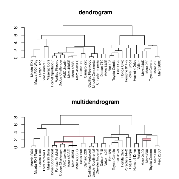
Figure 2: Pair-group dendrogram vs. variable-group multidendrogram. The ranges (rectangles) in the multidendrogram show the heterogeneity of distances within the group, but they are optional in the plots and can be hidden just by setting the col.rng argument in the plot() function to NULL.

The identification of ties requires the selection of the number of significant digits in the working dataset. For example, if the original distances are experimentally obtained with a resolution of three decimal digits, two distances that differ in the sixth decimal digit should be considered as equal. If this is not taken into account, ties might be broken just by the numerical imprecision inherent to computer representations of real numbers. In the linkage() function, you can control this level of resolution by adjusting its digits argument.

3 Linkage methods

3.1 Common linkage methods

During each iteration of the AHC algorithm, the distances $D(X_{I},X_{J})$ have to be computed between any two clusters $X_{I}=\bigcup_{i\in I}X_{i}$ and $X_{J}=\bigcup_{j\in J}X_{j}$, each one of them made up of several subclusters $X_{i}$ and $X_{j}$ indexed by $i$ in $I=\{i_{1},\ldots,i_{p}\}$ and $j$ in $J=\{j_{1},\ldots,j_{q}\}$, respectively. Lance and Williams (1966) introduced a formula for integrating several AHC linkage methods into a single system, avoiding the need of a separate computer program for each one of them. Similarly, Fernández and Gómez (2008) gave a variable-group generalization of this formula, compatible with the fusion of more than two clusters simultaneously:

$$D(X_{I},X_{J})=\sum_{i\in I}\sum_{j\in J}\alpha_{ij}D(X_{i},X_{j})+\sum_{i\in I}\sum_{\begin{subarray}{c}i^{\prime}\in I\\ i^{\prime}>i\end{subarray}}\beta_{ii^{\prime}}D(X_{i},X_{i^{\prime}})+\sum_{j\in J}\sum_{\begin{subarray}{c}j^{\prime}\in J\\ j^{\prime}>j\end{subarray}}\beta_{jj^{\prime}}D(X_{j},X_{j^{\prime}})\,.$$ (1)

Function linkage() in package mdendro uses this recurrence relation to compute the distance $D(X_{I},X_{J})$ from the distances $D(X_{i},X_{j})$ obtained during the previous iteration, being unnecessary to look back at the initial distance matrix $d(x_{i},x_{j})$ at all. The values of the parameters $\alpha_{ij}$, $\beta_{ii^{\prime}}$ and $\beta_{jj^{\prime}}$ determine the nature of the AHC linkage methods (Fernández and Gómez, 2008). Some of these methods even have weighted and unweighted forms, which differ in the weights assigned to individuals and clusters during the agglomerative process: weighted methods assign equal weights to clusters, while unweighted methods assign equal weights to individuals. Package mdendro implements weighted and unweighted forms of the most commonly used AHC linkage methods, namely:

• single: the proximity between clusters equals the minimum distance or the maximum similarity between objects.

• complete: the proximity between clusters equals the maximum distance or the minimum similarity between objects.

• arithmetic: the proximity between clusters equals the arithmetic mean proximity between objects. Also known as average linkage, UPGMA (unweighted pair-group method using averages) or WPGMA (weighted pair-group method using averages).

• centroid: the distance between clusters equals the square of the Euclidean distance between the centroids of each cluster. Also known as UPGMC (unweighted pair-group method using centroids) or WPGMC (weighted pair-group method using centroids). This method is available only for distance data.

• ward: the distance between clusters is a weighted squared Euclidean distance between the centroids of each cluster. This method is available only for distance data.

In Figure 3, we can see the differences between these AHC linkage methods on the UScitiesD dataset, a matrix of distances between a few US cities:

R> par(mfrow = c(2, 3))R> methods <- c("single", "complete", "arithmetic", "centroid", "ward")R> for (m in methods) {+    lnk <- linkage(UScitiesD, method = m)+    plot(lnk, cex = 0.6, main = m)+  }

Figure 3: Common linkage methods on the UScitiesD dataset.

3.2 Descriptive measures

The result of the linkage() function is an object of class ‘linkage’ that describes the resulting dendrogram obtained. In particular, this object contains the following calculated descriptors:

• cor: Cophenetic correlation coefficient (Sokal and Rohlf, 1962), defined as the Pearson correlation coefficient between the output cophenetic proximity data and the input proximity data. It is a measure of how faithfully the dendrogram preserves the pairwise proximity between objects.

• sdr: Space distortion ratio (Fernández and Gómez, 2020), calculated as the difference between the maximum and minimum cophenetic proximity data, divided by the difference between the maximum and minimum initial proximity data. Space dilation occurs when the space distortion ratio is greater than 1.

• ac: Agglomerative coefficient (Rousseeuw, 1986), a number between 0 and 1 measuring the strength of the clustering structure obtained.

• cc: Chaining coefficient (Williams et al., 1966), a number between 0 and 1 measuring the tendency for clusters to grow by the addition of clusters much smaller rather than by fusion with other clusters of comparable size.

• tb: Tree balance (Fernández and Gómez, 2020), a number between 0 and 1 measuring the equality in the number of leaves in the branches concerned at each fusion in the hierarchical tree.

For instance, when we use the linkage() function to calculate the complete linkage of the UScitiesD dataset, we obtain the following summary for the resulting dendrogram:

R> lnk <- linkage(UScitiesD, method = "complete")R> summary(lnk)

Call:linkage(prox = UScitiesD,        type.prox = "distance",        digits = 0,        method = "complete",        group = "variable")Binary dendrogram: TRUEDescriptive measures:      cor       sdr        ac        cc        tb0.8077859 1.0000000 0.7738478 0.3055556 0.9316262

While multidendrograms are unique, users may obtain structurally different pair-group dendrograms by just reordering the data. As a consequence, descriptors are invariant to permutations for multidendrograms, but not for pair-group dendrograms. Let us calculate a variable-group multidendrogram and a pair-group dendrogram for the same data:

R> cars <- round(dist(scale(mtcars)), digits = 1)R> lnk1 <- linkage(cars, method = "complete", group = "variable")R> lnk2 <- linkage(cars, method = "complete", group = "pair") Now, if we apply a random permutation to data:

R> set.seed(1234)R> ord <- sample(attr(cars, "Size"))R> carsp <- as.dist(as.matrix(cars)[ord, ord])R> lnk1p <- linkage(carsp, method = "complete", group = "variable")R> lnk2p <- linkage(carsp, method = "complete", group = "pair") We can check that the original and the permuted cophenetic correlation coefficients are identical for variable-group multidendrograms:

R> c(lnk1$cor, lnk1p$cor)

[1] 0.7782257 0.7782257 And they are different for pair-group dendrograms:

R> c(lnk2$cor, lnk2p$cor)

[1] 0.7780010 0.7776569

3.3 Parametric linkage methods

Two of the AHC linkage methods available in package mdendro, flexible and versatile, depend on a parameter that takes values in $[-1,+1]$ for flexible linkage, and in $(-\mathrm{Inf},+\mathrm{Inf})$ for versatile linkage. In function linkage(), the desired value for the parameter is passed through the par.method argument. Here come some examples on the UScitiesD dataset (see Figure 4):

R> par(mfrow = c(2, 3))R> vals <- c(-0.8, 0.0, 0.8)R> for (v in vals) {+    lnk <- linkage(UScitiesD, method = "flexible", par.method = v)+    plot(lnk, cex = 0.6, main = sprintf("flexible (%.1f)", v))+  }R> vals <- c(-10.0, 0.0, 10.0)R> for (v in vals) {+    lnk <- linkage(UScitiesD, method = "versatile", par.method = v)+    plot(lnk, cex = 0.6, main = sprintf("versatile (%.1f)", v))+  }

Figure 4: Parametric linkage methods on the UScitiesD dataset.

3.3.1 $\beta$-flexible linkage

Based on Equation 1, Lance and Williams (1967) proposed an infinite system of AHC strategies defined by the following constraint:

$$\underbrace{\sum_{i\in I}\sum_{j\in J}\alpha_{ij}}_{\alpha}+\underbrace{\sum_{i\in I}\sum_{\begin{subarray}{c}i^{\prime}\in I\\ i^{\prime}>i\end{subarray}}\beta_{ii^{\prime}}+\sum_{j\in J}\sum_{\begin{subarray}{c}j^{\prime}\in J\\ j^{\prime}>j\end{subarray}}\beta_{jj^{\prime}}}_{\beta}=1\,,$$ (2)

where $-1\leq\beta\leq+1$. Given a value of $\beta$, the value for $\alpha_{ij}$ can be assigned following a weighted approach as in the original $\beta$-flexible clustering method based on WPGMA and introduced by Lance and Williams (1966), or it can be assigned following an unweighted approach as in the $\beta$-flexible clustering method based on UPGMA and introduced by Belbin et al. (1992). Further details can be consulted in Fernández and Gómez (2020). When $\beta$ is set equal to $0$, flexible linkage is equivalent to arithmetic linkage.

It is interesting to know how the descriptive measures depend on the parameter of the parametric linkage methods. Package mdendro provides the function descplot() for this task. For example, using the flexible linkage method on the UScitiesD dataset (see Figure 5):

R> par(mfrow = c(2, 3))R> measures <- c("cor", "sdr", "ac", "cc", "tb")R> vals <- seq(from = -1, to = +1, by = 0.1)R> for (m in measures)+    descplot(UScitiesD, method = "flexible",+             measure = m, par.method = vals,+             type = "o",  main = m, col = "blue")

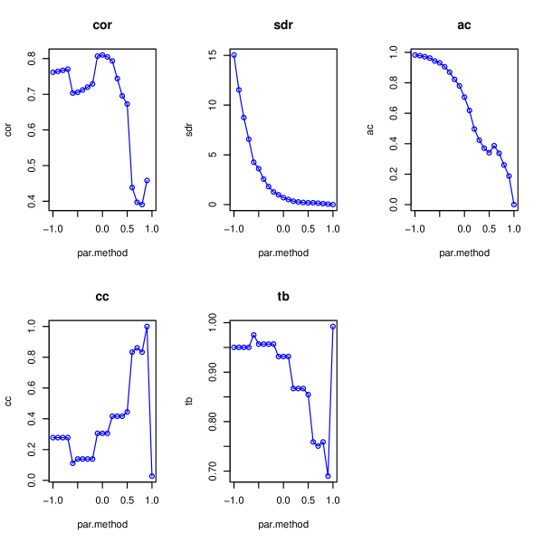
Figure 5: Descriptive measures obtained with the flexible linkage method on the UScitiesD dataset.

3.3.2 Versatile linkage

Package mdendro also implements another parametric linkage method named versatile linkage (Fernández and Gómez, 2020). Substituting the arithmetic means by generalized means, also known as power means, we can extend arithmetic linkage to any finite power $p\neq 0$:

$$D_{p}(X_{I},X_{J})=\left(\frac{1}{|X_{I}||X_{J}|}\sum_{i\in I}\sum_{j\in J}|X_{i}||X_{j}|[D_{p}(X_{i},X_{j})]^{p}\right)^{1/p}\,,$$ (3)

where $|X_{i}|$ and $|X_{j}|$ are the number of individuals in subclusters $X_{i}$ and $X_{j}$, and $|X_{I}|$ and $|X_{J}|$ are the number of individuals in clusters $X_{I}$ and $X_{J}$, i.e., $|X_{I}|=\sum_{i\in I}|X_{i}|$ and $|X_{J}|=\sum_{j\in J}|X_{j}|$. Equation 3 shows that versatile linkage can be calculated using a combinatorial formula from the distances $D_{p}(X_{i},X_{j})$ obtained during the previous iteration, in the same way as the recurrence formula given in Equation 1.

Versatile linkage provides a way of obtaining an infinite number of AHC strategies from a single formula, just changing the value of the power $p$. The decision of what power $p$ to use can be taken in agreement with the type of distance employed to measure the initial distances between individuals. For instance, if the initial distances were calculated using a generalized distance of order $p$, then the natural AHC strategy would be versatile linkage with the same power $p$. However, this procedure does not guarantee that the dendrogram obtained is the best one according to other criteria, e.g., cophenetic correlation coefficient, space distortion ratio or tree balance (see Section 3.2). Another possible approach consists in scanning the whole range of parameters $p$, calculate the preferred descriptors of the corresponding dendrograms, and decide if it is better to substitute the natural parameter $p$ by another one. This is especially important when only the distances between individuals are available, without coordinates for the individuals, as is common in multidimensional scaling problems, or when the distances have not been calculated using generalized means.

As in the case of flexible linkage, the parameter $p$ of versatile linkage is introduced using the par.method argument of the function linkage(). Here, it is also interesting to know how the descriptors depend on the parameter of this method (see Figure 6):

R> par(mfrow = c(2, 3))R> measures <- c("cor", "sdr", "ac", "cc", "tb")R> vals <- c(-Inf, (-20:+20), +Inf)R> for (m in measures)+    descplot(UScitiesD, method = "versatile",+             measure = m, par.method = vals,+             type = "o",  main = m, col = "blue")

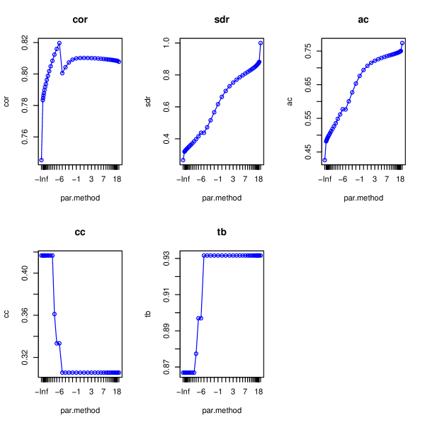
Figure 6: Descriptive measures obtained with the versatile linkage method on the UScitiesD dataset.

Particular cases. The generalized mean contains several well-known particular cases, depending on the value of the power $p$. Some of them reduce versatile linkage to the most commonly used methods, while others emerge naturally as deserving special attention:

• In the limit when $p\rightarrow-\infty$, versatile linkage becomes single linkage:

  $$D_{\min}(X_{I},X_{J})=\min_{i\in I}\,\min_{j\in J}\,D_{\min}(X_{i},X_{j})\,.$$ (4)

• In the limit when $p\rightarrow+\infty$, versatile linkage becomes complete linkage:

  $$D_{\max}(X_{I},X_{J})=\max_{i\in I}\,\max_{j\in J}\,D_{\max}(X_{i},X_{j})\,.$$ (5)

There are also three other particular cases that can be grouped together as Pythagorean linkages, which show the convenience to rename average linkage as arithmetic linkage, to emphasize the existence of different types of averages:

• When $p=+1$, the generalized mean is equal to the arithmetic mean and arithmetic linkage is recovered.

• When $p=-1$, the generalized mean is equal to the harmonic mean and harmonic linkage is obtained.

  $$D_{\mathrm{har}}(X_{I},X_{J})=\left(\frac{1}{|X_{I}||X_{J}|}\sum_{i\in I}\sum_{j\in J}|X_{i}||X_{j}|[D_{\mathrm{har}}(X_{i},X_{j})]^{-1}\right)^{-1}\,.$$ (6)

• In the limit when $p\rightarrow 0$, the generalized mean tends to the geometric mean and geometric linkage is obtained:

  $$D_{\mathrm{geo}}(X_{I},X_{J})=\left(\prod_{i\in I}\prod_{j\in J}[D_{\mathrm{geo}}(X_{i},X_{j})]^{|X_{i}||X_{j}|}\right)^{1/(|X_{I}||X_{J}|)}\,.$$ (7)

The correspondence between versatile linkage and the above mentioned linkage methods is summarized in Table 1.

	versatile (par.method)
complete	+Inf
arithmetic	+1
geometric	0
harmonic	-1
single	-Inf

Table 1: Correspondence between versatile linkage and other linkage methods.

Let us show a small example in which we plot different dendrograms as we increase the versatile linkage parameter, indicating the corresponding named methods (see Figure 7):

R> d = as.dist(matrix(c( 0,  7, 16, 12,+                        7,  0,  9, 19,+                       16,  9,  0, 12,+                       12, 19, 12, 0), nrow = 4))R> par(mfrow = c(2, 3))R> vals <- c(-Inf, -1, 0, 1, Inf)R> names <- c("single", "harmonic", "geometric", "arithmetic", "complete")R> titles <- sprintf("versatile (%.1f) = %s", vals, names)R> for (i in 1:length(vals)) {+    lnk <- linkage(d, method = "versatile", par.method = vals[i], digits = 2)+    plot(lnk, ylim = c(0, 20), cex = 0.6, main = titles[i])+  }

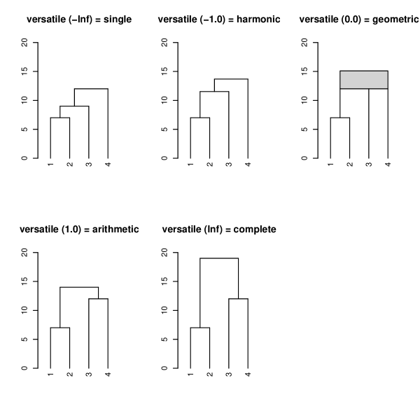
Figure 7: Example of different dendrograms obtained as we increase the versatile linkage parameter.

4 Comparison with other packages

Except for the cases containing tied distances, the equivalences in Table 2 hold between function linkage() in package mdendro, function hclust() in package stats and function agnes() in package cluster.

linkage()	hclust()	agnes()
single	single	single
complete	complete	complete
arithmetic, U	average	average
arithmetic, W	mcquitty	weighted
geometric, U/W	—	—
harmonic, U/W	—	—
versatile, U/W, $p$	—	—
—	ward	—
ward	ward.D2	ward
centroid, U	centroid	—
centroid, W	median	—
flexible, U, $\beta$	—	gaverage, $\beta$
—	—	gaverage, $\alpha_{1}$, $\alpha_{2}$, $\beta$, $\gamma$
flexible, W, $\beta$	—	flexible, $(1-\beta)/2$
—	—	flexible, $\alpha_{1}$, $\alpha_{2}$, $\beta$, $\gamma$

Table 2: Equivalences between functions linkage(), hclust() and agnes(). When relevant, weighted (W) or unweighted (U) versions of the linkage methods and the values for par.method are indicated.

For comparison, we can construct the same AHC using the functions linkage(), hclust() and agnes(), where the default plots just show some differences in aesthetics (see Figure 8):

R> lnk <- mdendro::linkage(UScitiesD, method = "complete")R> hcl <- stats::hclust(UScitiesD, method = "complete")R> agn <- cluster::agnes(UScitiesD, method = "complete")R> par(mar = c(5, 3, 4, 0), mfrow = c(1, 3))R> plot(lnk)R> plot(hcl)R> plot(agn, which.plots = 2)

Figure 8: Comparison of complete linkage on the UScitiesD dataset, using the functions linkage(), hclust() and agnes().

To enhance usability and interoperability, class ‘linkage’ includes the method as.dendrogram() for class conversion. In the previous example, converting to class ‘dendrogram’ the objects returned by the functions linkage(), hclust() and agnes(), we can see that all three dendrograms are structurally equivalent.

The cophenetic or ultrametric matrix is readily available as component coph of the returned ‘linkage’ object, and coincides with those obtained using the functionshclust() and agnes():

R> hcl.coph <- cophenetic(hcl)R> all(lnk$coph == hcl.coph)

[1] TRUE

R> agn.coph <- cophenetic(agn)R> all(lnk$coph == agn.coph)

[1] TRUE

The coincidence also applies to the cophenetic correlation coefficient and the agglomerative coefficient, with the advantage that function linkage() has both of them already calculated:

R> hcl.cor <- cor(UScitiesD, hcl.coph)R> all.equal(lnk$cor, hcl.cor)

[1] TRUE

R> all.equal(lnk$ac, agn$ac)

[1] TRUE

Plots including ranges are only available if you directly use the plot.linkage() function from package mdendro. Anyway, you may still take advantage of other dendrogram plotting packages, such as dendextend (Galili, 2015) and ape (Paradis and Schliep, 2019) (see Figure 9):

R> par(mar = c(5, 2, 4, 0), mfrow = c(1, 2))R> cars <- round(dist(scale(mtcars)), digits = 1)R> lnk <- linkage(cars, method = "complete")R> lnk.dend <- as.dendrogram(lnk)R> plot(dendextend::set(lnk.dend, "branches_k_color", k = 4),+       main = "dendextend package",+       nodePar = list(cex = 0.4, lab.cex = 0.5))R> lnk.hcl <- as.hclust(lnk)R> pal4 <- c("red", "forestgreen", "purple", "orange")R> clu4 <- cutree(lnk.hcl, 4)R> plot(ape::as.phylo(lnk.hcl),+       type = "fan",+       main = "ape package",+       tip.color = pal4[clu4],+       cex = 0.5)

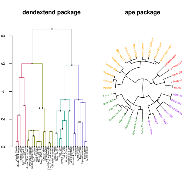
Figure 9: Converting objects of class ‘linkage’ using the function as.dendrogram(), one can take advantage of other dendrogram plotting packages, such as dendextend and ape.

And users can also use the function linkage() to plot heatmaps containing multidendrograms (see Figure 10):

R> heatmap(scale(mtcars), hclustfun = linkage)

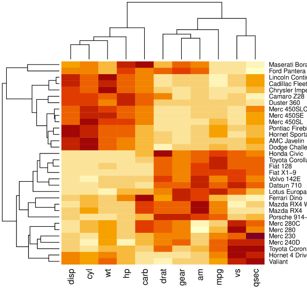
Figure 10: Example of heatmap constructed using the function linkage().

In addition, it is possible to work directly with similarity data without having to convert them to distances, provided they are in the range [0.0, 1.0]. A typical example would be a matrix of nonnegative correlations (see Figure 11):

R> sim <- as.dist(Harman23.cor$cov)R> lnk <- linkage(sim, type.prox = "sim")R> plot(lnk)

Figure 11: Example of a dendrogram constructed from a matrix of nonnegative correlations, i.e., directly using similarities instead of distances.

5 Summary and discussion

mdendro is a simple yet powerful R package to make hierarchical clusterings of data. It implements a variable-group algorithm for AHC that solves the nonuniqueness problem found in pair-group algorithms. This problem consists in obtaining different hierarchical clusterings from the same matrix of pairwise distances, when two or more shortest distances between different clusters are equal during the agglomeration process. In such cases, selecting a unique clustering can be misleading. Software packages that do not ignore this problem fail to adopt a common standard with respect to ties, and many of them simply break ties in any arbitrary way.

Package mdendro computes dendrograms grouping more than two clusters at the same time when ties occur. It includes and extends the functionality of other reference packages in several ways:

• Native handling of both distance and similarity matrices.

• Calculation of variable-group multifurcated dendrograms, which solve the nonuniqueness problem of AHC when there are tied distances.

• Implementation of the most common AHC linkage methods: single linkage, complete linkage, average linkage, centroid linkage and Ward’s method.

• Implementation of two parametric linkage methods: $\beta$-flexible linkage and versatile linkage. The latter leads naturally to the definition of two new linkage methods: harmonic linkage and geometric linkage.

• Implementation of both weighted and unweighted forms for the previous linkage methods.

• Calculation of the cophenetic (or ultrametric) matrix.

• Calculation of five descriptive measures for the resulting dendrogram: cophenetic correlation coefficient, space distortion ratio, agglomerative coefficient, chaining coefficient and tree balance.

• Plots of the descriptive measures for the parametric linkage methods.

Although ties need not be present in the initial proximity data, they may arise during the agglomerative process. For this reason, and given that the results of the variable-group algorithm coincide with those of the pair-group algorithm when there are no ties, we recommend to directly use package mdendro. With a single action one knows whether ties exist or not, and additionally the subsequent hierarchical clustering is obtained.

Computational details

The results in this paper were obtained using R 4.3.1 with the mdendro 2.1.0 package. R itself and all packages used are available from the Comprehensive R Archive Network (CRAN) at https://CRAN.R-project.org/.

References

- Almadanim et al. (2007) Almadanim M, Baleiras-Couto M, Pereira H, Carneiro L, Fevereiro P, Eiras-Dias J, Morais-Cecilio L, Viegas W, Veloso M (2007). “Genetic Diversity of the Grapevine (Vitis Vinifera L.) Cultivars Most Utilized for Wine Production in Portugal.” Vitis, 46(3), 116. 10.5073/vitis.2007.46.116-119.
- Arnau et al. (2005) Arnau V, Mars S, Marín I (2005). “Iterative Cluster Analysis of Protein Interaction Data.” Bioinformatics, 21(3), 364–378. 10.1093/bioinformatics/bti021.
- Backeljau et al. (1996) Backeljau T, De Bruyn L, De Wolf H, Jordaens K, Van Dongen S, Winnepennincks B (1996). “Multiple UPGMA and Neighbor-Joining Trees and the Performance of Some Computer Packages.” Molecular Biology and Evolution, 13(2), 309–313. 10.1093/oxfordjournals.molbev.a025590.
- Belbin et al. (1992) Belbin L, Faith D, Milligan G (1992). “A Comparison of Two Approaches to Beta-Flexible Clustering.” Multivariate Behavioral Research, 27(3), 417–433. 10.1207/s15327906mbr2703_6.
- Bezanson et al. (2017) Bezanson J, Edelman A, Karpinski S, Shah V (2017). “\proglangJulia: A Fresh Approach to Numerical Computing.” SIAM Review, 59(1), 65–98. 10.1137/141000671.