Machine Learning-Aided First-Principles Calculations of Redox Potentials

Abstract

Redox potentials of electron transfer reactions are of fundamental importance for the performance and description of electrochemical devices. Despite decades of research, accurate computational predictions for the redox potential of even simple metals remain very challenging. Here we use a combination of first principles calculations and machine learning to predict the redox potentials of three redox couples, $\mathrm{Fe}^{2+}$/$\mathrm{Fe}^{3+}$, $\mathrm{Cu}^{+}$/$\mathrm{Cu}^{2+}$ and $\mathrm{Ag}^{+}$/$\mathrm{Ag}^{2+}$. Using a hybrid functional with a fraction of 25% exact exchange (PBE0) the predicted values are 0.92, 0.26 and 1.99 V in good agreement with the best experimental estimates (0.77, 0.15, 1.98 V). We explain in detail, how we combine machine learning, thermodynamic integration from machine learning to semi-local functionals, as well as a combination of thermodynamic perturbation theory and $\Delta$-machine learning to determine the redox potentials for computationally expensive hybrid functionals. The combination of these approaches allows one to obtain statistically accurate results.

I Introduction

Green energy and a circular economy are one of the key paradigms that our human society needs to realize in the next few decades. This implies that we need to give up on the combustion of fossil fuels. A key element to achieve this paradigm shift is the use of electrochemistry, be it for batteries and fuel cells, to convert electrical energy to hydrogen or other valuable chemicals, or to convert hydrogen back to energy without direct combustion in air. The redox potential of electron transfer (ET), $\mathrm{Ox}+n\mathrm{e}^{-}\rightarrow\mathrm{Red}$ in liquids, is an essential property for a variety of electrochemical energy conversion devices, such as batteries, fuel cells, and electrochemical fuel synthesis. It determines the alignment of redox levels relative to the Fermi level of a metal, or valence band maximum (VBM) and conduction band minimum (CBM) of semiconductor and insulator electrodes. It also determines the potential windows of ions and molecules in solutions, that is the range of voltages within which a specific ion or molecule can undergo electrochemical reactions. This information is vital to design redox species and solvent molecules, such as redox couples for redox-flow batteries WeberJApplElectrochm_2011 , solvents and additives for Li-ion batteries Ong_ChemMater_2011 ; Xu_ChemRev_2014 ; Haregewoin_EnergyEnvironSci_2016 , radical scavengers for fuel cells Zaton_SusEnergyFuel_2017 and electrocatalysts for fuel synthesis Pinaud_EnergyEnvSci_2013 ; Morikawa_ACR_2022 . Unfortunately up to date, accurate first-principles (FP) predictions of this key property are difficult to come by, with typical prediction errors being 0.5 V. For instance, Sprik and co-workers Adriaanse_JCPL_2012 ; Liu_JPCB_2015 , found a large spread of values for two metal ion couples, with values between $-1.13$ and $-0.20$ V for $\mathrm{Cu}^{+}$/$\mathrm{Cu}^{2+}$ (exp. 0.16 V) and 0.90 and 1.72 V for $\mathrm{Ag}^{+}$/$\mathrm{Ag}^{2+}$ (exp. 1.98 V) with variations being related to differences in the density functional, pseudopotential, but also code base (CMPD versus CP2K). Although the "best" values using hybrid functionals and highly accurate pseudopotentials are reasonably close to experiment ($-0.20$ V for Cu, and 1.72 V for Ag), the agreement is still far from quantitative.

Table 1: Redox potentials $U_{\mathrm{redox}}$ of three transition metal cations calculated by RPBE+D3, PBE0 (0.25), PBE0 (0.50), PBE0+D3 (0.25) and PBE0+D3 (0.50) using MLFF and $\Delta$-ML. Here, values in the parenthesis are the fraction of the exact exchange. The results for 64 water molecular systems are tabulated. The absolute potential of SHE is set to 4.44 V Trasatti_PAC_1986 . The root means square errors (RMSE) compared to the experimental redox potentials are also shown.

XC functional	Fe	Cu	Ag	RMSE
RPBE+D3	0.80	0.66	1.88	0.29
PBE0 (0.25)	0.92	0.26	1.99	0.11
PBE0 (0.50)	0.79	$-$0.34	2.12	0.30
PBE0+D3 (0.25)	0.94	0.24	2.02	0.11
PBE0+D3 (0.50)	0.83	$-$0.38	2.13	0.32
Exp.[a]	0.77	0.15	1.98

[a] From Ref. bard_book_1985 .

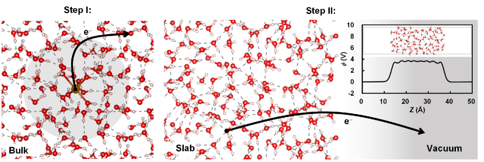
Figure 1: Conceptual steps to oxidize the reduced state by transferring an electron from the metal ion to the vacuum: the transfer from the redox level to an oxygen 1s level far from the reactant in the bulk in the same super cell (Step I) and the electron transfer from an oxygen 1s level in the slab to the vacuum (Step II). White small spheres, red medium spheres and large spheres with other colors are H, O and metal atoms, respectively. The figure inset shows the snapshot of the water slab and computed local potential profile across the water slab. The graphics showing bulk and interfacial models are made by VESTA Momma_JAC_2011 .

The main goals of the present work are three-fold: First, we want to accurately calculate the redox potential of metal ions in water for three prototypical cases: Ag, Cu, and Fe. Ag²⁺ ions are among the most aggressive oxidants with a large redox potential, whereas the redox potential of Cu²⁺ ions is fairly shallow, and the $\mathrm{Fe}^{2+}$/$\mathrm{Fe}^{3+}$ reaction lies in between. The first two redox reactions involve large changes in the ion water coordination, which makes the calculation challenging, whereas the redox reaction of Fe is a so called simple outer sphere ET reaction and has been the subject of numerous experimental and theoretical studies Marcus_RevModPhys_1993 . The Fe ions are conceived to be particularly challenging for density functional theory. Second, we want to establish a computationally feasible pathway that yields statistically accurate results. Last but not least, we want to systematically explore different density functionals to set a guideline for future studies.

II Overview of modelling

We start with an overview of the used theoretical modelling. The Nernst equation implies that the redox potential $U_{\mathrm{redox}}$ is determined by the free energy difference $\Delta F$ between the reduced and oxidized states as

$$U_{\mathrm{redox}} =-\frac{\Delta F}{en},$$ (1)

where $e$ is the elementary charge and $n$ is the number of electrons involved in the reaction. The free energy difference $\Delta F$ can be exactly determined by thermodynamic integration (TI)Zwanzig_JCP_1954 ; Kirkwood_JCP_1935

$$\Delta F =\int_{0}^{1}\left<\frac{\partial H}{\partial\lambda}\right>_{\lambda}d\lambda.$$ (2)

Here, $\langle A\rangle_{\lambda}$ denotes the expectation value of $A$ for an ensemble created by the Hamiltonian at coupling $\lambda$. The integral seamlessly connects the oxidized state ($\lambda=0$) to the reduced state ($\lambda=1$) along a coupling path Blumberger_JCP_2006 ; Dorner_PRL_2018 . If the structural changes are significant from the oxidized to the reduced species — recall that this is the case for Ag and Cu — many integration steps are required to accurately determine the energy difference. The application of this approach entails two difficulties. (i) Clearly, it implies huge computational cost if applied directly to hybrid functionals; if 100.000 timesteps are required, several 10 mio core hours are necessary to obtain good statistical accuracy. (ii) Second, during the reaction one electron needs to be transferred to a reservoir, characterizing the chemical potential of the electrons. In experiment that redox potential is usually measured with respect to the vacuum level, a quantity not directly accessible during a simulation using periodic boundary conditions.

Chemical potential of electrons: We will address the second point (ii) first. Jiao and co-workers Jiao_JCTC_2011 suggested to use the average electrostatic potential as suitable reference point, and Leung Leung_JPCL_2010 calculated the position of the average electrostatic potential with respect to the vacuum level in a second independent calculation involving a water slab. We refine this approach in a conceptually easy to understand way that simultaneously reduces finite size errors. During the redox reactions, we use the 1s level of oxygen atoms far away from the reactant as conceptual reference. The first principles code used in the present work (VASP) conveniently calculates this reference point for each atom in the simulation cell. This means that the energy contribution $\frac{\partial H}{\partial\lambda}$ is replaced by the more appropriate $\frac{\partial H}{\partial\lambda}-\mu\frac{\partial N_{\mathrm{e}}}{\partial\lambda}$, where $N_{\mathrm{e}}$ is the electronic number of the system, and $\mu$ is the chemical potential that we fix to be the energy of the O 1s level. In practice, the average position of the O 1s level varies slowly and smoothly along the coupling path, so we can replace the integral $\int\left<\mu\right>d\lambda$ by the average of the O 1s levels in the fully reduced and oxidized state (trapezoidal rule). In the second step, we conceptually transfer the electron from the O 1s level to the vacuum level. This implies that we calculate the electrostatic potential in the middle of the vacuum (vacuum level) and subtract from this the average O 1s level of water molecules in the middle of a water slab. The scheme is illustrated in Fig. 1. One key advantage of using machine learned (ML) force fields for this step is that one can create many statistically independent configurations for the water slab. We do this by on-the-fly learning an H₂O force field for the bulk and then for the surface, and performing finally extensive million step ML molecular dynamics for the surface. From this simulation we draw 3000 statistically independent snapshots. Only for these snapshots, first principles calculations are performed to determine the average O 1s level with respect to the vacuum level. This greatly accelerates the calculations but maintains excellent statistical accuracy. We finally note that using atoms far away from the "defect" as reference, also helps to reduce finite size effects Lany_PRB_2008 ; Freysoldt_RMP_2014 .

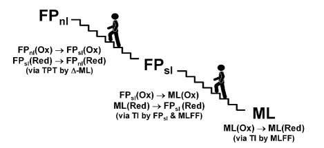
Figure 2: Schematic of ML-aided TI and TPT to compute the free energy difference $\Delta F_{\mathrm{bulk}}$. See details of equations in the Methods section.

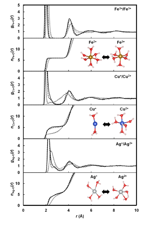
Figure 3: Metal-oxygen radial distribution functions ($g_{\mathrm{X-O}}$) and running integration numbers ($n_{\mathrm{X-O}}$) provided by 100 ps MLFF-MD and 10 ps FPMD simulations. Gray and black lines are for the reduced and oxidized states, respectively. Solid and dashed lines are results obtained by the MLFF and FP_sl, respectively. Graphics in the insets show first solvation structures at the reduced and oxidized states.

Thermodynamic integration: Determining the free energy difference, i.e. point (i), is somewhat more difficult to address. Naively, one could just perform the required thermodynamic integration using ML surrogate models. As we will show below this yields only acceptable accuracy. Hence, one still needs to perform thermodynamic integration from the ML surrogate model to the first principles calculations, for both the oxidized as well as the reduced state. We will adopt this strategy for semi-local functions. So this involves three calculations: thermodynamic integration from the oxidised to the reduces species using a ML surrogate model, and then for each oxidation state, integration from MLFF to the first principles Hamiltonian. There is one final obstacle though: performing thermodynamic integration to a hybrid functional that includes non-local exchange is still exceedingly demanding and challenging. So in this specific case, we have decided to replace the integration by thermodynamic perturbation theory (TPT),

$$\Delta F =F_{1}-F_{0}=-\frac{1}{\beta}\mathrm{ln}\left<e^{-\beta\Delta U}\right>_{0}=-\frac{1}{\beta}\mathrm{ln}\left<e^{\beta\Delta U}\right>_{1},$$ (3)

where the symbol $\Delta U$ denotes the potential energy difference between the two end points. Although equation Eq. (3) is in principle exact, the potential energy difference might need to be evaluated for thousands or even many ten thousand configurations if the ensembles generated by the two potentials are too distinct. However, TPT has the distinct advantage that the configurations can be generated using the cheap Hamiltonian. In our case, we use Eq. (3) to determine the free energy difference between a cheap semi-local functional and a hybrid functional. A further key advance is to learn the difference $\Delta U$ between the semi-local functional and the non-local hybrid functional, that is, we adopt $\Delta$-machine learning ($\Delta$-ML) Balabin_JCP_2009 ; Ramakrishnan_JCTC_2015 ; Bartok_PRB_2013 ; Chmiela_NatCommun_2018 ; Sauceda_JCP_2019 ; Liu_2022_PRB ; Carla_PRM_2023 ; Liu_PRL_2023 . Since the energy difference between the semi-local functional and the non-local functional is very smooth, few tens of hybrid functional calculations are sufficient to learn a highly accurate ML representation of $\Delta U$. The computational cost is ultimately only limited by generating sufficient configurations using the semi-local functional.

III Results and discussion

We now detail our results, and will show that the adopted procedure yields statistically highly accurate results. The calculations were performed using VASP Kresse_PRB_1996 ; Kresse_CMS_1996 and the projector augmented wave (PAW) method Blochl_PRB_1994 ; Kresse_PRB_1999 . For the ML force fields (MLFFs) the implementation detailed in previous publications is used Jinnouchi_PRB_2019 ; Jinnouchi_JPCL_2020 ; Jinnouchi_JPCL_2023 . Similar to the pioneering ML approaches Behler_PRL_2007 ; Bartok_PRL_2010 ; Bartok_PRB_2013 , the potential energy in our MLFF method is approximated as a summation of local energies [see Eq. (17)]. The local energy is approximated as a weighted sum of kernel basis functions [see Eq. (18)]. A Bayesian formulation allows to efficiently predict energies, forces and stress tensor components as well as their uncertainties. The predicted uncertainty enables the reliable sampling of the reference structures on-the-fly during the FPMD simulation. Details of the equations, parameters and training conditions are summarized in the Methods section and Section S3 in Supplementary Information (SI). As in the previous studies Jinnouchi_PRL_2019 ; Jinnouchi_PRB_2019 ; Jinnouchi_PRB_2020 ; Jinnouchi_JCP_2020 , the MLFFs trained on a semi-local functional with dispersion corrections achieve root mean square errors (RMSEs) of 1-5 meV atom^-1 and 0.04-0.11 eV Å^-1 for energies and forces as shown in Table S2. The three ET reactions are examined in water by using a semi-local Hammer_PRB_1999 functional with a dispersion correction Grimme_JCP_2010 ; Grimme_JCC_2011 (RPBE+D3) and hybrid functionals Adamo_JCP_1999 with and without a dispersion correction (PBE0 and PBE0+D3). Systematic comparisons of different functionals help us to study the effects of the exact exchange as well as dispersion corrections. As shown in Table 1 [see lines of PBE0 (0.25) and PBE0+D3 (0.25)] good agreement with experiment is achieved using the hybrid functional with 1/4 exact exchange, regardless of whether dispersion corrections are used or not.

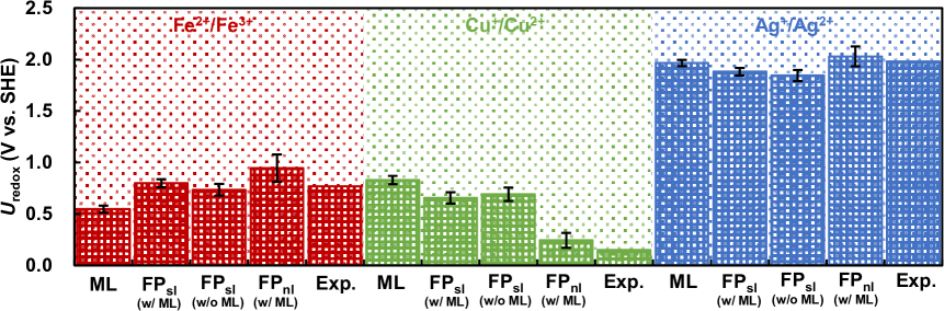
Figure 4: Computed and experimental redox potentials. ML means the results obtained by the MLFF trained on $\mathrm{FP_{sl}}$ (RPBE+D3) without any correction. The small letters ‘w/ ML’ under $\mathrm{FP_{sl}}$ mean that the ML result was corrected by the scheme shown in Fig. 2. The letters ‘w/o ML’ mean the result calculated by $\mathrm{FP_{sl}}$ using Eqs.(15) and (16) without MLFF. Here, $\mathrm{FP_{nl}}$ means PBE0+D3 (0.25) result obtained by the scheme shown in Fig. 2. Experimental values are taken from Ref. bard_book_1985 .

In the following we will use the abbreviations $\mathrm{FP_{nl}}$(Ox/Red), $\mathrm{FP_{sl}}$(Ox/Red), and ML(Ox/Red) to denote calculations using a non-local hybrid functional, a semi-local functional and machine-learned FF for the oxidized and reduced cases, respectively. Figure 2 summarizes the steps schematically, and further details can be found in the Methods section. The ML-aided integration has four significant advantages as summarized below:

• The integration $\mathrm{ML}$ (Ox) $\rightarrow$ $\mathrm{ML}$ (Red) using the MLFF takes into account most of the non-linear components of the integrand in the TI (see Figs. S1 and S2 in SI). Excellent statistical accuracy can be reached for this step.

• The MLFFs also provide well-equilibrated initial structures required for other calculational steps.

• The integrands in $\mathrm{FP_{sl}}$ (Ox) $\rightarrow$ $\mathrm{ML}$ (Ox) and $\mathrm{ML}$ (Red) $\rightarrow$ $\mathrm{FP_{sl}}$ (Red) are small and almost linear in the coupling parameter (see Fig. S3) owing to the accurate reproduction of the $\mathrm{FP_{sl}}$ structures by the MLFF (see Fig. 3 and Table S2). Hence, these demanding integrals (evaluation of $\mathrm{FP_{sl}}$ calculation in every MD step) converge using a few tens of pico second MD simulations.

• The expensive $\mathrm{FP_{nl}}$ free energy calculation is accelerated by many orders of magnitude by $\Delta$-ML, that quickly predicts energy differences on thousands of structures from $\mathrm{FP_{nl}}$ data but requires only a few tens of training structures (see Table S3 and Fig. S5). The high efficiency allows for excellent statistics despite using TPT (see Fig. S4).

Water surface calculations: For RPBE+D3, the present MLFF provides a surface tension of 79$\pm$5 mN m^-1 for the 128 molecular system and 84$\pm$5 mN m^-1 for the 1024 molecular system at 298 K. The results are slightly larger than the value of 68$\pm$2 mN m^-1 calculated by a neural network potential Wohlfahrt_JCP_2020 and experimental value of 72 mN m^-1 Vargaftik_JCP_1983 while it is within the range (50-90 mN m^-1) of previous MD results by FP Ohto_JCTC_2019 and classical force fields Taylor_JCP_1996 ; Vega_JCP_2007 . Distributions of interfacial water dipole moments for both, 128 and 1024 molecular systems, are shown in Fig. S6. They consistently indicate that the orientation of interfacial water molecules is bimodal as reported in previous MD studies employing the classical SPC/E force field Taylor_JCP_1996 . The distributions are also consistent with the results of sum frequency generation (SFG) analyses Du_PRL_1993 .

Metal water coordination: Figure 3 shows metal-oxygen radial distribution functions (RDFs) and running integration numbers (RINs) at the reduced and oxidized states calculated by the MLFF and FP_sl methods. The MLFFs well reproduce RDFs and RINs of the FP_sl method. Both methods show that the coordination number of Fe ions is 6 independent of the charge state. In contrast, the value for Cu changes from 2-3 in the reduced state (Cu⁺) to 5-6 in the oxidized state (Cu²⁺). The coordination number of Ag also changes from 4-5 in the reduced state (Ag⁺) to 5-6 in the oxidized state (Ag²⁺). These hydration structures agree with the ones reported in previous MD studies using FPMD methods Remsungen_CPL_2004 ; Blumberger_JACS_2004 ; Bogatko_JPCA_2010 and empirical force fields Remsungen_CPL_2004 . Although there are slight deviations in the Fe-O distance and shoulders for Cu-O and Ag-O in the RDFs likely related to the short FPMD simulation time and errors in the MLFFs, overall, our MLFFs reproduce the first-principles energies and structures of the hydrated metal cations with good accuracy.

Redox potentials: After verifying the size effect on the redox potentials of $\mathrm{FP_{sl}}$ by using unit cells containing 32, 64 and 96 water molecules (see $U_{\mathrm{redox}}$ in Fig. S8), calculations were conducted on the bulk solutions containing 64 water molecules in the unit cell. The computed redox potentials are compared with the experimental ones in Fig. 4. All relevant data ($\Delta F_{\mathrm{bulk}}$ and $\Delta\phi$), as well as results of other functionals with error bars, are summarized in Section S5. The MLFFs trained on $\mathrm{FP_{sl}}$ (RPBE+D3) (see ML in Fig. 4) lead to non-negligible deviations of 0.19 V on average from the values of a full $\mathrm{FP_{sl}}$ calculations without any MLFF (see $\mathrm{FP_{sl}}$ w/o ML). The deviations can be corrected by two TI integrations [$\mathrm{FP_{sl}}$(Ox) $\rightarrow$ $\mathrm{ML}$(Ox) and $\mathrm{ML}$(Red) $\rightarrow$ $\mathrm{FP_{sl}}$(Red) in Fig. 2] as shown by $\mathrm{FP_{sl}}$ w/ ML. However, the semi-local functional result in fairly large and non-systematic errors. For Ag the redox potential is underestimated, whereas for Cu it is significantly overestimated compared to experiment.

The errors can be significantly decreased to 0.11 V on average using hybrid functionals with one quarter exact exchange. As tabulated in Table 1, $U_{\mathrm{redox}}$ for the Cu⁺/Cu²⁺ couple decreases with increasing fraction of the exact exchange, whereas the redox potential for the Ag⁺/Ag²⁺ couple increases with increasing the fraction. For Fe²⁺/Fe³⁺, the trend is not so clear (first increase then slight decrease).

Overall the present trends agree with the results obtained using semi-local and hybrid functionals as reported by Liu and co-workers Liu_JPCB_2015 . However, likely because of insufficient statistical accuracy (or local basis set errors), the previous results were less accurate. Finally, the effects of Grimme’s dispersion correction is small for all redox couples. This implies that changes of the electronic properties (such as water valence band maximum and conduction band minimum) are most relevant, whereas all the functionals give a similar and good account of the solvation structure.

In summary, our approach enables efficient statistical sampling that is indispensable for accurate computations of the free energies of aqueous systems. The TI and TPT calculations allow to improve the accuracy from the ML model to the semi-local functional and from the semi-local functional to the hybrid functional step-by-step. Combining TPT and $\Delta$-machine learning are particularly promising, since this allows to obtain statistically highly accurate results even for expensive functionals in very little compute time. For instance, it is well conceivable that one could also use methods beyond density functional theory for the final step. Our final results reproduce the redox potentials of the three transition metal cations with excellent accuracy using a standard hybrid functional. The integration pathways chosen here are generalizable to a wide variety of electron transfer reactions. We believe that the scheme will pave the way to first-principles electrochemistry predicting the key property of redox reactions in energy conversion devices.

IV Methods

IV.1 TI and TPT

The TI and TPT shown in Fig. 2 in the main text is conducted by using the equations listed below.

• $\mathbf{FP_{nl}(Ox)\rightarrow FP_{sl}(Ox)}$

$$-\Delta F_{0}^{\mathrm{FP_{nl}-FP_{sl}}} \simeq-\left<\Delta U_{0}^{\mathrm{\Delta ML}}\right>_{\mathrm{FP_{sl}}}$$

$$+\frac{\beta}{2}\left<\left(\Delta U_{0}^{\mathrm{\Delta ML}}-\left<\Delta U_{0}^{\mathrm{\Delta ML}}\right>_{\mathrm{FP_{sl}}}\right)^{2}\right>_{\mathrm{FP_{sl}}}.$$ (4)

• $\mathbf{FP_{sl}(Ox)\rightarrow ML(Ox)}$

$$-\Delta F_{0}^{\mathrm{FP_{sl}-ML}} =-\int_{0}^{1}\left<\frac{\partial H_{0}^{\mathrm{FP_{sl}-ML}}}{\partial\eta}\right>_{\eta}d\eta,$$ (5)

$$H_{0}^{\mathrm{FP_{sl}-ML}} =\sum\limits_{i=1}^{N_{\mathrm{a}}}\frac{\left|\mathbf{p}_{i}\right|^{2}}{2m_{i}}+\eta U_{0}^{\mathrm{FP_{sl}}}+\left(1-\eta\right)U_{0}^{\mathrm{ML}}.$$ (6)

• $\mathbf{ML(Ox)\rightarrow ML(Red)}$

$$\Delta F^{\mathrm{ML}} =\int_{0}^{1}\left<\frac{\partial H^{\mathrm{ML}}}{\partial\lambda}\right>_{\lambda}d\lambda,$$ (7)

$$H^{\mathrm{ML}} =\sum\limits_{i=1}^{N_{\mathrm{a}}}\frac{\left|\mathbf{p}_{i}\right|^{2}}{2m_{i}}+\lambda U_{1}^{\mathrm{ML}}+\left(1-\lambda\right)U_{0}^{\mathrm{ML}}.$$ (8)

• $\mathbf{ML(Red)\rightarrow FP_{sl}(Red)}$

$$\Delta F_{1}^{\mathrm{FP_{sl}-ML}} =\int_{0}^{1}\left<\frac{\partial H_{1}^{\mathrm{FP_{sl}-ML}}}{\partial\eta}\right>_{\eta}d\eta,$$ (9)

$$H_{1}^{\mathrm{FP_{sl}-ML}} =\sum\limits_{i=1}^{N_{\mathrm{a}}}\frac{\left|\mathbf{p}_{i}\right|^{2}}{2m_{i}}+\eta U_{1}^{\mathrm{FP_{sl}}}+\left(1-\eta\right)U_{1}^{\mathrm{ML}}.$$ (10)

• $\mathbf{FP_{sl}(Red)\rightarrow FP_{nl}(Red)}$

$$\Delta F_{1}^{\mathrm{FP_{nl}-FP_{sl}}} \simeq\left<\Delta U_{1}^{\mathrm{\Delta ML}}\right>_{\mathrm{FP_{sl}}}$$

$$-\frac{\beta}{2}\left<\left(\Delta U_{1}^{\mathrm{\Delta ML}}-\left<\Delta U_{1}^{\mathrm{\Delta ML}}\right>_{\mathrm{FP_{sl}}}\right)^{2}\right>_{\mathrm{FP_{sl}}}.$$ (11)

Here, $N_{\mathrm{a}}$ is the number of atoms, and $m_{i}$ and $\mathbf{p}_{i}$ are the mass and momentum vector of $i$-th atom. The symbols $U_{\mu}^{\mathrm{FP_{nl}}}$, $U_{\mu}^{\mathrm{FP_{sl}}}$ and $U_{\mu}^{\mathrm{ML}}$ are the potential energies for the oxidized ($\mu=0$) and reduced ($\mu=1$) states calculated by the non-local functional, semi-local functional and MLFF trained on the semi-local functional, respectively. The symbol $\Delta U_{\mu}^{\mathrm{\Delta ML}}$ denotes the potential energy difference calculated by the $\Delta$-ML model trained on the potential energy difference $U_{\mu}^{\mathrm{FP_{nl}}}-U_{\mu}^{\mathrm{FP_{sl}}}$ between the non-local and semi-local functionals. In Eqs. (4) and (11), the second-order cumulant expansion is employed. The expansion is exact if the probability distribution of $\Delta U_{\mu}^{\mathrm{\Delta ML}}$ is Gaussian. The condition is reasonably satisfiled as shown later in this subsection.

The free energy differences $\Delta F_{\mathrm{bulk}}$ of the $\mathrm{ML}$, $\mathrm{FP_{sl}}$ and $\mathrm{FP_{nl}}$ methods are obtained as

$$\Delta F_{\mathrm{bulk}}^{\mathrm{ML}} =\Delta F^{\mathrm{ML}},$$ (12)

$$\Delta F_{\mathrm{bulk}}^{\mathrm{FP_{sl}}} =\Delta F_{\mathrm{bulk}}^{\mathrm{ML}}+\Delta F_{1}^{\mathrm{FP_{sl}-ML}}-\Delta F_{0}^{\mathrm{FP_{sl}-ML}},$$ (13)

$$\Delta F_{\mathrm{bulk}}^{\mathrm{FP_{nl}}} =\Delta F_{\mathrm{bulk}}^{\mathrm{FP_{sl}}}+\Delta F_{1}^{\mathrm{FP_{nl}-FP_{sl}}}-\Delta F_{0}^{\mathrm{FP_{nl}-FP_{sl}}}.$$ (14)

To validate the MLFF-aided computations of the free energy difference $\Delta F_{\mathrm{bulk}}^{\mathrm{FP_{sl}}}$, the same property was also computed by the TI without using the $\mathrm{ML}$ method:

$$\Delta F^{\mathrm{FP_{sl}}} =\int_{0}^{1}\left<\frac{\partial H^{\mathrm{FP_{sl}}}}{\partial\lambda}\right>_{\lambda}d\lambda,$$ (15)

$$H^{\mathrm{FP_{sl}}} =\sum\limits_{i=1}^{N_{\mathrm{a}}}\frac{\left|\mathbf{p}_{i}\right|^{2}}{2m_{i}}+\lambda U_{1}^{\mathrm{FP_{sl}}}+\left(1-\lambda\right)U_{0}^{\mathrm{FP_{sl}}},$$ (16)

For the TI calculation in Eq. (7), the trapezoidal rule with equidistant five points was used following the previous FP study by Blumberger and co-workers Blumberger_JCP_2006 . For each point, the ensemble average was taken over an 80-ps-NVT-ensemble MD simulation at 298 K after a 20 ps equilibration. Similar to the MLFF calculations, the trapezoidal rule with equidistant five points was used for the TI calculation in Eq. (15). For each grid, the ensemble average was taken over a 20-ps-MD simulation starting from the final structure of the TI calculation using the MLFF at the same grid point. Each initial structure of the MD simulations was prepared by annealing the system from 400 K to 298 K by a 100-ps-NVT-ensemble MD simulation using the MLFF after annealing the same system from 1000 K to 400 K by a 1-ns-NVT ensemble MD simulation using the polymer consistent force field (PCFF) Sun_JCC_1994 implemented in a homemade MD program Jinnouchi_ECA_2016 . Figures S1 and S2 in SI show the integrands of Eqs. (7) and (15), respectively, as functions of the coupling parameter $\lambda$. In the same figures, probability distributions of $\Delta U^{\mathrm{ML}}=U_{1}^{\mathrm{ML}}-U_{0}^{\mathrm{ML}}$ and $\Delta U^{\mathrm{FP_{sl}}}=U_{1}^{\mathrm{FP_{sl}}}-U_{0}^{\mathrm{FP_{sl}}}$ at each $\lambda$ are also shown. For all redox couples, the variance of the distribution varies with changing $\lambda$, and thus, the integrand is non-linear with respect to $\lambda$ [see Eq. (S6) in SI]. Hence, the second cumulant expansion Eq. (S4) is not applicable to the whole integration from the oxidized state to the reduced state.

The TI calculations in Eqs. (5) and (9) were conducted using the trapezoidal rule with three equidistant points. At each point, a 10-ps-NVT-ensemble MD simulation at 298 K was performed. The integrands shown in Fig. S3 are smaller than the ones shown in Figs. S1 and S2, respectively. They are also nearly proportional to the coupling parameter $\eta$.

In the TPT calculations using the $\Delta$-ML models, the ensemble average in each of Eqs. (4) and (11) was taken over 1400 configurations selected randomly from 70-ps-NVT-ensemble FPMD simulations using the FP_sl method. Although these FPMD simulations are expensive, the overall computational time is still much smaller than full FP simulations. To ensure the applications of the second-order cumulant expansion, we show the probability distributions of the energy difference $\Delta U_{\mu}^{\mathrm{\Delta ML}}$ in Fig. S4. The distribution are well fitted by Gaussian functions, indicating that Eqs. (4) and (11) are reasonable approximations.

The MD simulations were performed using a Langevin thermostat Allen_Book_2008 . For efficient sampling, the mass of hydrogen and time step were set to 2 a.u. and 1 fs.

IV.2 MLFF and $\mathrm{\Delta}$-ML

Similar to previous machine-learning approaches Behler_PRL_2007 ; Bartok_PRL_2010 , the potential energy $U$ of a structure with $N_{\mathrm{a}}$ atoms in our MLFF method is approximated as a summation of local energies $U_{i}$ written as

$$U =\sum\limits_{i=1}^{N_{\mathrm{a}}}U_{i}.$$ (17)

Following the Gaussian approximation potential pioneered by Bártok and co-workers Bartok_PRL_2010 , the local energy $U_{i}$ is approximated as a weighted sum of functions $K\left(\mathbf{x}_{i},\mathbf{x}_{i_{\mathrm{B}}}\right)$ centered at reference points $\{\mathbf{x}_{i_{\mathrm{B}}}|i_{\mathrm{B}}=1,...,N_{\mathrm{B}}\}$

$$U_{i} =\sum\limits_{i_{\mathrm{B}}=1}^{N_{\mathrm{B}}}w_{i_{\mathrm{B}}}K\left(\mathbf{x}_{i},\mathbf{x}_{i_{\mathrm{B}}}\right).$$ (18)

The coefficients $\{w_{i_{\mathrm{B}}}|i_{\mathrm{B}}=1,...,N_{\mathrm{B}}\}$ are optimized to best reproduce the FP energies, forces, and stress tensor components as obtained by the FPMD simulations. The descriptor $\mathbf{x}_{i}$ used in this study is a vector containing two and three body contributions Jinnouchi_JCP_2020 :

$$\mathbf{x}^{\mathrm{T}}_{i}\rightarrow\left(\sqrt{\beta^{(2)}}\mathbf{x}^{(2)\mathrm{T}}_{i},\sqrt{\beta^{(3)}}\mathbf{x}^{(3)\mathrm{T}}_{i}\right),$$ (19)

Here, $\beta^{(2)}$ and $\beta^{(3)}(=1-\beta^{(2)})$ are the weights on the two and three body descriptors, $\mathbf{x}_{i}^{(2)}$ and $\mathbf{x}_{i}^{(3)}$, respectively. The vectors $\mathbf{x}_{i}^{(2)}$ and $\mathbf{x}_{i}^{(3)}$ collect the expansion coefficients of two and three body distribution functions with respect to the orthonormal radial and angular basis sets Jinnouchi_PRB_2019 ; Jinnouchi_JCP_2020 :

$$\rho_{i}^{(2)}\left(r\right) =\frac{1}{\sqrt{4\pi}}\sum\limits_{n=1}^{N^{0}_{\mathrm{R}}}c^{i}_{n}\chi_{n0}\left(r\right)$$ (20)

$$\rho_{i}^{(3)}\left(r,s,\theta\right) =\sum\limits_{l=0}^{L_{\mathrm{max}}}\sum\limits_{n=1}^{N^{l}_{\mathrm{R}}}\sum\limits_{\nu=1}^{N^{l}_{\mathrm{R}}}\sqrt{\frac{2l+1}{2}}$$

$$\times p_{n\nu l}^{i}\chi_{nl}\left(r\right)\chi_{\nu l}\left(s\right)P_{l}\left(\mathrm{cos}\theta\right).$$ (21)

The two and three body distribution functions $\rho_{i}^{(2)}$ and $\rho_{i}^{(3)}$ are defined as:

$$\rho_{i}^{(2)}\left(r\right) =\frac{1}{4\pi}\int\rho_{i}\left(r\hat{\mathbf{r}}\right),$$ (22)

$$\rho_{i}^{(3)}\left(r,s,\theta\right) =\iint d\hat{\mathbf{r}}d\hat{\mathbf{s}}\;\delta\left(\hat{\mathbf{r}}\cdot\hat{\mathbf{s}}-\mathrm{cos}\theta\right)$$

$$\;\times\rho_{i}\left(r\hat{\mathbf{r}}\right)\rho_{i}\left(s\hat{\mathbf{s}}\right),$$ (23)

$$\rho_{i}\left(\mathbf{r}\right) =\sum\limits_{j=1}^{N_{\mathrm{a}}}f_{\mathrm{cut}}\left(\left|\mathbf{r}_{j}-\mathbf{r}_{i}\right|\right)g\left(\mathbf{r}-\left(\mathbf{r}_{j}-\mathbf{r}_{i}\right)\right)$$ (24)

The function $g$ is the smoothed $\delta$-function, and $f_{\mathrm{cut}}$ is a cutoff function that smoothly eliminates the contribution from atoms outside a given cutoff radius $R_{\mathrm{cut}}$. For $\chi_{nl}$ and $P_{l}$, normalized spherical Bessel functions $\chi_{nl}=j_{l}(q_{n}r)$ and Legendre polynomials of order $l$ are used in this work, respectively. For the kernel basis functions, the smooth overlap of atomic positions (SOAP) kernel Bartok_PRB_2013 is employed

$$K\left(\mathbf{x}_{i},\mathbf{x}_{i_{\mathrm{B}}}\right) =\left(\mathbf{\hat{x}}_{i}\cdot\mathbf{\hat{x}}_{i_{\mathrm{B}}}\right)^{\zeta}.$$ (25)

The hat symbol $\mathbf{\hat{x}}_{i}$ denotes a normalized vector of $\mathbf{x}_{i}$. The normalization and exponentiation in Eq. (25) introduce non-linear terms that mix two- and three-body contributions.

The same formulation is used for the $\mathrm{\Delta}$-ML method. In the $\mathrm{\Delta}$-ML method, differences of potential energies and forces between two FP methods, semi-local and non-local functionals in this study, are used as the training data.

Parameter sets of the descriptors and kernel basis functions used in previous publications were employed in this study Jinnouchi_PRB_2019 ; Jinnouchi_JCP_2020 ; Jinnouchi_JPCL_2023 . The parameters are tabulated in Table S1.

Bulk solutions were modeled by systems as shown in Fig. 1 in the main text. The number of water molecules was set to 32, 64, and 96. Three different model sizes were examined to clarify the system size effect. The sizes of the unit cells were set to obtain a water density of 0.99 g cm^-3 as found by MLFF calculations on a water slab (see Section S4 in SI). The size of the unit cell for the 32 water molecules is same as the one used in previous FPMD studies Blumberger_JACS_2004 ; Blumberger_JCP_2006 ; Adriaanse_JCPL_2012 ; Liu_JPCB_2015 . For each of the reduced and oxidized states, MLFF and $\Delta$-ML models were constructed. All MLFF models were generated on the fly during a 100-ps-NVT-MD simulation at 400 K by using the active-learning algorithm developed in our previous study Jinnouchi_PRB_2019 . The temperature for the training runs was set to a value higher than the target one of 298 K for production runs, to ensure that training data and kernel basis functions were provided in a wider phase space. A Langevin thermostat Allen_Book_2008 was used to control the temperature. Exchange-correlation interactions between electrons were described by the semi-local RPBE functional Hammer_PRB_1999 with Grimme’s D3 dispersion corrections Grimme_JCP_2010 ; Grimme_JCC_2011 . Root mean square errors (RMSEs) of the constructed MLFFs for energies, forces, and stress tensor components on test data are tabulated in Table S2. The RMSEs are similar to those of MLFFs used in previous studies Jinnouchi_PRL_2019 ; Jinnouchi_PRB_2019 ; Jinnouchi_PRB_2020 ; Jinnouchi_JCP_2020 .

After examining the system size effect using the semi-local functional, $\Delta$-ML models were constructed on systems containing 64 water molecules. Each $\Delta$-ML model was trained on FP energies and forces of 40 structures selected randomly from a trajectory of a 20 ps NVT-ensemble FPMD simulation at 298K. The FPMD simulation was performed using the RPBE+D3 functional. Differences in energies and forces between the non-local and semi-local functionals for these 40 structures were used as training data. PBE0 Adamo_JCP_1999 with and without the Grimme’s D3 dispersion correction Grimme_JCP_2010 ; Grimme_JCC_2011 was employed as the non-local functional because the functional is known to accurately predict properties of water Gaiduk_JCPL_2015 . The fraction of the exact exchange was set to 0.25 and 0.50 to determine how this influences the redox potentials. RMSEs of the $\Delta$-ML models on test structures are tabulated in Table S3. The RMSEs are one to two orders of magnitude smaller than the errors of the RPBE+D3 MLFFs tabulated in Table S2. Thanks to the remarkable accuracy of the $\Delta$-ML models in describing the energy difference between various FP methods, it is possible to obtain exceedingly accurate free energy differences between different FP methods using thermodynamic perturbation theory as shown in Fig. S5. This is one of the key advances of the present work.

The vacuum-water interface for the production run was modeled by a water slab composed of 128 water molecules per unit cell. Following the previous study Leung_JPCL_2010 , a rectangular cell of $12.5\times 12.5\times 50$ ų was employed. Similar to the MLFFs for the bulk systems, the MLFF for the interface was also generated by using the active-learning scheme. The systems used for the training were a water bulk composed of 64 water molecules in a $12.4\times 12.4\times 12.4$ ų cubic cell and slab composed of 64 water molecules in an $8.8\times 8.8\times 40.8$ ų rectangular cell. Training simulations for both the bulk and slab were performed by NVT-ensemble MD simulations at 300, 400, 600 and 800 K. As shown in Table S2, the constructed MLFF realizes small RMSEs on test data taken from a 100-ps-MD simulation of a water slab composed of 128 water molecules at 298 K.

The annealing procesure used for the production runs explained in the previous subsection was also used to prepare for the initial structures for the training runs. All FP calculations were performed using VASP Kresse_PRB_1996 ; Kresse_CMS_1996 . A 2$\times$2$\times$2 $\mathbf{k}$-point mesh was used for the bulk systems containing 32 water molecules. For other systems, $\Gamma$-point was used. Plane-wave cutoff energy was set to 520 eV. The PAW atomic reference configuration was 1s¹ for H, 2s²2p⁴ for O, 3d⁷4s¹ for Fe, 3d¹⁰4p¹ for Cu, and 4d¹⁰5s¹ for Ag. The parameters for the MD simulations are same as the ones described in the previous subsection.

Code availability

The VASP code is distributed by the VASP Software GmbH. The machine learning modules will be included in the release of vasp.6.3. Prerelease versions are available from G.K. upon reasonable request.

Data availability

The data that support the findings of this study are available from the corresponding author upon reasonable request.

References

- [1] Adam Z. Weber, Matthew M. Mench, Jeremy P. Meyers, Philip N. Ross, Jeffrey T. Gostick, and Qinghua Liu. Redox flow batteries: a review. Journal of Applied Electrochemistry, 41(10):1137–1164, Oct 2011.
- [2] Shyue Ping Ong, Oliviero Andreussi, Yabi Wu, Nicola Marzari, and Gerbrand Ceder. Electrochemical windows of room-temperature ionic liquids from molecular dynamics and density functional theory calculations. Chemistry of Materials, 23(11):2979–2986, Jun 2011.
- [3] Kang Xu. Electrolytes and interphases in li-ion batteries and beyond. Chemical Reviews, 114(23):11503–11618, Dec 2014.
- [4] Atetegeb Meazah Haregewoin, Aselefech Sorsa Wotango, and Bing-Joe Hwang. Electrolyte additives for lithium ion battery electrodes: progress and perspectives. Energy Environ. Sci., 9:1955–1988, 2016.
- [5] M. Zatoń, J. Roziere, and D. J. Jones. Current understanding of chemical degradation mechanisms of perfluorosulfonic acid membranes and their mitigation strategies: a review. Sustainable Energy Fuels, 1:409–438, 2017.
- [6] Blaise A. Pinaud, Jesse D. Benck, Linsey C. Seitz, Arnold J. Forman, Zhebo Chen, Todd G. Deutsch, Brian D. James, Kevin N. Baum, George N. Baum, Shane Ardo, Heli Wang, Eric Miller, and Thomas F. Jaramillo. Technical and economic feasibility of centralized facilities for solar hydrogen production via photocatalysis and photoelectrochemistry. Energy Environ. Sci., 6:1983–2002, 2013.
- [7] Takeshi Morikawa, Shunsuke Sato, Keita Sekizawa, Tomiko. M. Suzuki, and Takeo Arai. Solar-driven reduction using a semiconductor/molecule hybrid photosystem: From photocatalysts to a monolithic artificial leaf. Accounts of Chemical Research, 55(7):933–943, Apr 2022.
- [8] Christopher Adriaanse, Jun Cheng, Vincent Chau, Marialore Sulpizi, Joost VandeVondele, and Michiel Sprik. Aqueous redox chemistry and the electronic band structure of liquid water. The Journal of Physical Chemistry Letters, 3(23):3411–3415, Dec 2012.
- [9] Xiandong Liu, Jun Cheng, and Michiel Sprik. Aqueous transition-metal cations as impurities in a wide gap oxide: The / and / redox couples revisited. The Journal of Physical Chemistry B, 119(3):1152–1163, Jan 2015.
- [10] S. Trasatti. The absolute electrode potential: an explanatory note (recommendations 1986). Pure and Applied Chemistry, 58(7):955–966, 1986.
- [11] A.J. Bard, R. Parsons, and J. Jordan. Standard Potentials in Aqueous Solution. Monographs in Electroanalytical Chemistry and Electrochemistr. Taylor & Francis, 1985.
- [12] Koichi Momma and Fujio Izumi. 3 for three-dimensional visualization of crystal, volumetric and morphology data. Journal of Applied Crystallography, 44(6):1272–1276, 2011.
- [13] Rudolph A. Marcus. Electron transfer reactions in chemistry. theory and experiment. Rev. Mod. Phys., 65:599–610, Jul 1993.
- [14] Robert W. Zwanzig. High-temperature equation of state by a perturbation method. i. nonpolar gases. The Journal of Chemical Physics, 22(8):1420–1426, 1954.
- [15] John G. Kirkwood. Statistical mechanics of fluid mixtures. The Journal of Chemical Physics, 3(5):300–313, 1935.
- [16] Jochen Blumberger, Ivano Tavernelli, Michael L. Klein, and Michiel Sprik. Diabatic free energy curves and coordination fluctuations for the aqueous redox couple: A biased born-oppenheimer molecular dynamics investigation. The Journal of Chemical Physics, 124(6):064507, 2006.
- [17] Florian Dorner, Zoran Sukurma, Christoph Dellago, and Georg Kresse. Melting : Beyond density functional theory. Phys. Rev. Lett., 121:195701, Nov 2018.
- [18] Dian Jiao, Kevin Leung, Susan B. Rempe, and Tina M. Nenoff. First principles calculations of atomic nickel redox potentials and dimerization free energies: A study of metal nanoparticle growth. Journal of Chemical Theory and Computation, 7(2):485–495, Feb 2011.
- [19] Kevin Leung. Surface potential at the air-water interface computed using density functional theory. The Journal of Physical Chemistry Letters, 1(2):496–499, Jan 2010.
- [20] Stephan Lany and Alex Zunger. Assessment of correction methods for the band-gap problem and for finite-size effects in supercell defect calculations: Case studies for and . Phys. Rev. B, 78:235104, Dec 2008.
- [21] Christoph Freysoldt, Blazej Grabowski, Tilmann Hickel, Jörg Neugebauer, Georg Kresse, Anderson Janotti, and Chris G. Van de Walle. First-principles calculations for point defects in solids. Rev. Mod. Phys., 86:253–305, Mar 2014.
- [22] G. Kresse and J. Furthmüller. Efficient iterative schemes for ab initio total-energy calculations using a plane-wave basis set. Phys. Rev. B, 54:11169, 1996.
- [23] G. Kresse and J. Furthmüller. Efficiency of ab-initio total energy calculations for metals and semiconductors using a plane-wave basis set. Computational Materials Science, 6:15, 1996.
- [24] P. E. Blöchl. Projector augmented-wave method. Phys. Rev. B, 50:17953–17979, Dec 1994.
- [25] G. Kresse and D. Joubert. From ultrasoft pseudopotentials to the projector augmented-wave method. Phys. Rev. B, 59:1758–1775, Jan 1999.
- [26] Ryosuke Jinnouchi, Ferenc Karsai, and Georg Kresse. On-the-fly machine learning force field generation: Application to melting points. Phys. Rev. B, 100:014105, 2019.
- [27] Ryosuke Jinnouchi, Kazutoshi Miwa, Ferenc Karsai, Georg Kresse, and Ryoji Asahi. On-the-fly active learning of interatomic potentials for large-scale atomistic simulations. The Journal of Physical Chemistry Letters, 11(17):6946–6955, Sep 2020.
- [28] Ryosuke Jinnouchi, Saori Minami, Ferenc Karsai, Carla Verdi, and Georg Kresse. Proton transport in perfluorinated ionomer simulated by machine-learned interatomic potential. The Journal of Physical Chemistry Letters, 14(14):3581–3588, Apr 2023.
- [29] Jörg Behler and Michele Parrinello. Generalized neural-network representation of high-dimensional potential-energy surfaces. Phys. Rev. Lett., 98:146401, 2007.
- [30] Albert P. Bartók, Mike C. Payne, Risi Kondor, and Gábor Csányi. Gaussian approximation potentials: The accuracy of quantum mechanics, without the electrons. Phys. Rev. Lett., 104:136403, 2010.
- [31] Albert P. Bartók, Risi Kondor, and Gábor Csányi. On representing chemical environments. Phys. Rev. B, 87:184115, May 2013.
- [32] Ryosuke Jinnouchi, Jonathan Lahnsteiner, Ferenc Karsai, Georg Kresse, and Menno Bokdam. Phase transitions of hybrid perovskites simulated by machine-learning force fields trained on the fly with bayesian inference. Phys. Rev. Lett., 122:225701, 2019.
- [33] Ryosuke Jinnouchi, Ferenc Karsai, and Georg Kresse. Making free-energy calculations routine: Combining first principles with machine learning. Phys. Rev. B, 101:060201, Feb 2020.
- [34] Ryosuke Jinnouchi, Ferenc Karsai, Carla Verdi, Ryoji Asahi, and Georg Kresse. Descriptors representing two- and three-body atomic distributions and their effects on the accuracy of machine-learned inter-atomic potentials. The Journal of Chemical Physics, 152(23):234102, 2020.
- [35] B. Hammer, L. B. Hansen, and J. K. Nørskov. Improved adsorption energetics within density-functional theory using revised perdew-burke-ernzerhof functionals. Phys. Rev. B, 59:7413–7421, Mar 1999.
- [36] Stefan Grimme, Jens Antony, Stephan Ehrlich, and Helge Krieg. A consistent and accurate ab initio parametrization of density functional dispersion correction () for the 94 elements -. The Journal of Chemical Physics, 132(15):154104, 2010.
- [37] Stefan Grimme. Density functional theory with london dispersion corrections. WIREs Computational Molecular Science, 1(2):211–228, 2011.
- [38] Carlo Adamo and Vincenzo Barone. Toward reliable density functional methods without adjustable parameters: The model. The Journal of Chemical Physics, 110(13):6158–6170, 1999.
- [39] Roman M. Balabin and Ekaterina I. Lomakina. Neural network approach to quantum-chemistry data: Accurate prediction of density functional theory energies. The Journal of Chemical Physics, 131(7):074104, 2009.
- [40] Raghunathan Ramakrishnan, Pavlo O. Dral, Matthias Rupp, and O. Anatole von Lilienfeld. Big data meets quantum chemistry approximations: The -machine learning approach. Journal of Chemical Theory and Computation, 11(5):2087–2096, May 2015.
- [41] Stefan Chmiela, Huziel E. Sauceda, Klaus-Robert Müller, and Alexandre Tkatchenko. Towards exact molecular dynamics simulations with machine-learned force fields. Nature Communications, 9(1):3887, Sep 2018.
- [42] Huziel E. Sauceda, Stefan Chmiela, Igor Poltavsky, Klaus-Robert Müller, and Alexandre Tkatchenko. Molecular force fields with gradient-domain machine learning: Construction and application to dynamics of small molecules with coupled cluster forces. The Journal of Chemical Physics, 150(11):114102, 2019.
- [43] Peitao Liu, Carla Verdi, Ferenc Karsai, and Georg Kresse. Phase transitions of zirconia: Machine-learned force fields beyond density functional theory. Phys. Rev. B, 105:L060102, Feb 2022.
- [44] Carla Verdi, Luigi Ranalli, Cesare Franchini, and Georg Kresse. Quantum paraelectricity and structural phase transitions in strontium titanate beyond density functional theory. Phys. Rev. Mater., 7:L030801, Mar 2023.
- [45] Peitao Liu, Jiantao Wang, Noah Avargues, Carla Verdi, Andreas Singraber, Ferenc Karsai, Xing-Qiu Chen, and Georg Kresse. Combining machine learning and many-body calculations: Coverage-dependent adsorption of on (111). Phys. Rev. Lett., 130:078001, Feb 2023.
- [46] Oliver Wohlfahrt, Christoph Dellago, and Marcello Sega. Ab initio structure and thermodynamics of the water/vapor interface by neural-network molecular dynamics. The Journal of Chemical Physics, 153(14):144710, 2020.
- [47] N. B. Vargaftik, B. N. Volkov, and L. D. Voljak. International tables of the surface tension of water. Journal of Physical and Chemical Reference Data, 12(3):817–820, 1983.
- [48] Tatsuhiko Ohto, Mayank Dodia, Sho Imoto, and Yuki Nagata. Structure and dynamics of water at the water–air interface using first-principles molecular dynamics simulations within generalized gradient approximation. Journal of Chemical Theory and Computation, 15(1):595–602, Jan 2019.
- [49] Ramona S. Taylor, Liem X. Dang, and Bruce C. Garrett. Molecular dynamics simulations of the liquid/vapor interface of water. The Journal of Physical Chemistry, 100(28):11720–11725, Jan 1996.
- [50] C. Vega and E. de Miguel. Surface tension of the most popular models of water by using the test-area simulation method. The Journal of Chemical Physics, 126(15), 04 2007. 154707.
- [51] Q. Du, R. Superfine, E. Freysz, and Y. R. Shen. Vibrational spectroscopy of water at the vapor/water interface. Phys. Rev. Lett., 70:2313–2316, Apr 1993.
- [52] Tawun Remsungnen and Bernd M Rode. Molecular dynamics simulation of the hydration of transition metal ions: the role of non-additive effects in the hydration shells of and ions. Chemical Physics Letters, 385(5):491–497, 2004.
- [53] Jochen Blumberger, Leonardo Bernasconi, Ivano Tavernelli, Rodolphe Vuilleumier, and Michiel Sprik. Electronic structure and solvation of copper and silver ions: a theoretical picture of a model aqueous redox reaction. Journal of the American Chemical Society, 126(12):3928–3938, Mar 2004.
- [54] Stuart A. Bogatko, Eric J. Bylaska, and John H. Weare. First principles simulation of the bonding, vibrational, and electronic properties of the hydration shells of the high-spin ion in aqueous solutions. The Journal of Physical Chemistry A, 114(5):2189–2200, Feb 2010.
- [55] H. Sun. Force field for computation of conformational energies, structures, and vibrational frequencies of aromatic polyesters. Journal of Computational Chemistry, 15(7):752–768, 1994.
- [56] Ryosuke Jinnouchi, Kenji Kudo, Naoki Kitano, and Yu Morimoto. Molecular dynamics simulations on permeation through nafion ionomer on platinum surface. Electrochimica Acta, 188:767–776, 2016.
- [57] M. P. Allen and D. J. Tildesley. Computer Simulation of Liquids. 1987.
- [58] Alex P. Gaiduk, François Gygi, and Giulia Galli. Density and compressibility of liquid water and ice from first-principles simulations with hybrid functionals. The Journal of Physical Chemistry Letters, 6(15):2902–2908, Aug 2015.