Whitham modulation theory and two-phase instabilities for generalized nonlinear Schrödinger equations with full dispersion

Abstract

The generalized nonlinear Schrödinger equation with full dispersion (FDNLS) is considered in the semiclassical regime. The Whitham modulation equations are obtained for the FDNLS equation with general linear dispersion and a generalized, local nonlinearity. Assuming the existence of a four-parameter family of two-phase solutions, a multiple-scales approach yields a system of four independent, first order, quasi-linear conservation laws of hydrodynamic type that correspond to the slow evolution of the two wavenumbers, mass, and momentum of modulated periodic traveling waves. The modulation equations are further analyzed in the dispersionless and weakly nonlinear regimes. The ill-posedness of the dispersionless equations corresponds to the classical criterion for modulational instability (MI). For modulations of linear waves, ill-posedness coincides with the generalized MI criterion, recently identified by Amiranashvili and Tobisch [5]. A new instability index is identified by the transition from real to complex characteristics for the weakly nonlinear modulation equations. This instability is associated with long-wavelength modulations of nonlinear two-phase wavetrains and can exist even when the corresponding one-phase wavetrain is stable according to the generalized MI criterion. Another interpretation is that, while infinitesimal perturbations of a periodic wave may not grow, small but finite amplitude perturbations may grow, hence this index identifies a nonlinear instability mechanism for one-phase waves. Classifications of instability indices for multiple FDNLS equations with higher order dispersion, including applications to finite depth water waves and the discrete NLS equation are presented and compared with direct numerical simulations.

1 Introduction

We study the full-dispersion nonlinear Schrödinger (FDNLS) equation

$$i\psi_{t}=\widetilde{\Omega}(-i\partial_{x})\psi+f^{\prime}(|\psi|^{2})\psi~{},$$ (1)

where the pseudo-differential operator $\widetilde{\Omega}(-i\partial_{x})$ captures full linear dispersion, whose action is defined through the Fourier transform as

$$\widetilde{\Omega}\left(-i\partial_{x}\right)\psi(x,t)\equiv\frac{1}{2\pi}\int_{\mathbb{R}}\Omega(\xi)e^{i\xi x}\int_{\mathbb{R}}\psi(x^{\prime},t)e^{-i\xi x^{\prime}}\,\mathrm{d}x^{\prime}\,\mathrm{d}\xi~{},\quad$$

where $\Omega(\xi)$ is a smooth, real-valued dispersion relation. The function $f$ in (1) is a smooth, generalized nonlinearity. The classical, cubic NLS equation with second-order dispersion is the special case of (1) with $\Omega(\xi)=\frac{1}{2}\xi^{2}$ and $f(\rho)=\sigma\rho^{2}/2$, i.e.,

$$i\psi_{t}=-\frac{1}{2}\psi_{xx}+\sigma|\psi|^{2}\psi,\quad\sigma=\pm 1~{}.$$ (2)

The NLS equation (2) is a universal model of the slowly varying (weakly dispersive) and weakly nonlinear envelope of a monochromatic wave train [1, 61].

The formulation of the FDNLS equation is similar to the modeling approach that was pioneered by Whitham in the context of shallow water waves [75]. The Whitham equation

$$u_{t}+uu_{x}+\widetilde{\Omega}\left(-i\partial_{x}\right)u=0,$$ (3)

incorporates weak nonlinearity and the full linear dispersion of unidirectional water waves with phase speed $\Omega(k)=\sqrt{\tanh k}$ and corresponding pseudo-differential operator defined by the symbol $\widetilde{\Omega}(-i\partial_{x})=\sqrt{\tan(-i\partial_{x})}$. Equation (3) has been shown to be a superior model when approximating the Euler equations [59] and experiments [70, 21] compared to the Korteweg-de Vries (KdV) equation in the shallow water regime where $\widetilde{\Omega}\left(-i\partial_{x}\right)u\sim u_{x}+u_{xxx}/6$. Whitham’s idea is natural from a modeling standpoint and has since been generalized to other physical scenarios and model equations, primarily in the context of single- or multi-layer fluids [50, 55, 3, 52, 30, 44, 14]. In the same spirit, we view the FDNLS equation (1) as a generic weakly nonlinear, strongly dispersive modulation equation for one-phase wavetrains, which has been used in various applications such as water waves [72] and optics [5].

The NLS equation (2) is the canonical model for weakly-dispersive deep water waves [81, 1]. However, higher-order dispersive effects can be significant for deep water waves [32, 73, 72, 65, 66, 55], such as for oceanic rogue waves (also known as freak waves or peaking waves) that exhibit steep, cusp-like profiles [31, 6]. Higher-order generalied NLS models are also significant in other applications. In particular, higher-order dispersive effects are significant for ultrashort optical pulses [4] where the propagation of intense laser pulses in optical fibers have been studied for more than 30 years (cf. [64, 4]). In that context, the measured spectrum of optical fibers corresponds to $\Omega(\xi)$. Example experimental studies on short-wave effects that are not captured by the NLS equation (2) include radiative effects in optical fibers [24, 25, 57] and longitudinal soliton tunneling in dispersion-shifted fibers [58]. Stronger dispersion has been used to predict the appearance of new types of optical instabilities [82, 5].

A powerful mathematical tool for analyzing modulations of nonlinear waves is Whitham modulation theory [76]. Whitham modulation theory describes the slow evolution of nonlinear wavetrains by a system of quasi-linear, first order partial differential equations for the wave parameters known as the Whitham modulation equations—plural so as not to be confused with the singular Whitham equation (3). The Whitham equations are used to describe long wavelength modulations of strongly nonlinear wavetrains, hence can be viewed as a large amplitude generalization of the classical NLS equation (2), albeit without dispersive corrections [61]. One of the earliest applications of modulation theory was to the studies of modulational instability (MI) of nonlinear periodic traveling waves in optics [69, 13, 62] and water waves [10, 9]. Around the same time, it was recognized that the ellipticity, hence ill-posedness of the initial value problem, of the Whitham modulation equations implies MI [76]. See [80] for a more detailed history.

In this work, we consider long wavelength modulations of both one- and two-phase solutions of the FDNLS equation (1). Assuming the existence of two-phase solutions, we obtain the Whitham modulation equations in a general form for slow spatio-temporal variation of the solution’s parameters. We then obtain approximate two-phase solutions and analyze the corresponding modulation equations in more detail. We determine their hyperbolicity and a new two-phase modulational instability index that determines whether small amplitude, long-wavelength perturbations of the two-phase solution grow. When the dispersion $\Omega(\xi)$ is cubic, quartic, from finite depth water waves, or from the discrete NLS equation, we identify regimes where the periodic, one-phase solution is modulationally stable but the two-phase solution is modulationally unstable. This result implies nonlinear instability, i.e., that appropriately selected small but finite amplitude perturbations of the one-phase solution grow even though infinitesimal, linear perturbations do not.

In order to set the stage for the modulation and stability analysis of FDNLS solutions, we now briefly review modulation theory and modulational instability for the cubic NLS equation (2).

1.1 Modulation theory

The simplest one-phase solution of Eq. (2) is

$$\psi(x,t)=\sqrt{\bar{\rho}}e^{i\theta},\quad\theta=\overline{u}x-\gamma t,\quad\gamma=\frac{1}{2}\overline{u}^{2}+\sigma\bar{\rho},\quad\bar{\rho}>0,\quad\overline{u}\in\mathbb{R},$$ (4)

where $\bar{\rho}=|\psi|^{2}$ is the square modulus, $\overline{u}=i(\psi_{x}^{*}\psi-\psi_{x}\psi^{*})/\bar{\rho}$ is the wavenumber ($\psi^{*}$ is the complex conjugate of $\psi$), and $\gamma$ is the frequency. These quantities admit a hydrodynamic interpretation in which $\bar{\rho}$ and $\overline{u}$ are analogous to the fluid density and velocity, respectively [46]. The solution (4) is often referred to as the Stokes wave, owing to its derivation by Stokes in the context of weakly nonlinear water waves [68].

Modulation equations for the Stokes solution’s parameters $(\bar{\rho},\overline{u})$ can be obtained with the WKB-like, multiscale ansatz [76]

$$\psi(x,t)=\sqrt{\bar{\rho}(X,T)}e^{i\theta}+\epsilon\psi_{1}(\theta,X,T)+\cdots,$$ (5)

where $X=\epsilon x$, $T=\epsilon t$ and

$$\theta=S/\epsilon,\quad\theta_{x}=S_{X}=\overline{u}(X,T),\quad\theta_{t}=S_{T}=-\gamma(X,T),\quad 0<\epsilon\ll 1.$$ (6)

This ansatz is then inserted into Eq. (2) and like powers of $\epsilon$ are equated. At leading order, we obtain the same frequency relation as in (4), but now applicable locally $\gamma(X,T)=\tfrac{1}{2}\overline{u}(X,T)^{2}+\sigma\bar{\rho}(X,T)$. Combining solvability at $\mathcal{O}(\epsilon)$ over the space of $2\pi$-periodic functions in $\theta$ for $\psi_{1}(\theta,X,T)$ and the compatibility condition $S_{XT}=S_{TX}$ yields the modulation equations, also known as the shallow water equations,

$$\bar{\rho}_{T}+(\bar{\rho}\overline{u})_{X} =0,$$ (7a)

$$\overline{u}_{T}+\left(\tfrac{1}{2}\overline{u}^{2}+\sigma\bar{\rho}\right)_{X} =0~{}.$$ (7b)

The characteristic velocities of the shallow water equations (7) are

$$\lambda_{1,2} =\overline{u}\pm\sqrt{\sigma\bar{\rho}}~{}.$$ (8)

Equations (7) describe large amplitude, nonlinear modulations. When $\sigma=1$, the modulation equations are hyperbolic. As such, smooth initial data can develop a gradient catastrophe in finite time, which is regularized by higher-order dispersive effects not included in (7). This regularization can be achieved by incorporating an additional phase into modulation theory that results in the formation of a dispersive shock wave [34, 39]. When $\sigma=-1$, the characteristic velocities (8) are complex and the initial value problem is ill-posed. Nevertheless, the evolution of certain initial data that leads to singularity formation can also be regularized by appealing to additional modulation phases [36, 38, 15].

The NLS equation (2) admits exact solutions in terms of Jacobi elliptic functions. The solutions take the form

$$\psi(x,t)=\sqrt{\rho(\theta_{2})}\exp\left(i\theta_{1}+i\int_{0}^{\theta_{2}}u(s)ds\right),$$ (9)

where $\theta_{1}=\overline{u}x-\gamma t$, $\theta_{2}=kx-\omega t$, $\rho(\theta)$ is a $2\pi$-periodic function, and $u(\theta)$ is a mean-zero, $2\pi$-periodic function. The form of the solutions for $\sigma=\pm 1$ are well documented, see, e.g., [51]. Since (9) is periodic in two independent phases $\theta_{1}$ and $\theta_{2}$, it is called a two-phase solution. The phase $\theta_{1}$ is sometimes referred to as trivial because it corresponds to the Stokes wave background (4) when $\rho(\theta)=\bar{\rho}$ and $u(\theta)=0$ are constant.

The modulation equations for the parameters of the two-phase solution family (9) have been derived in both cases $\sigma=\pm 1$ [40, 63]. They can be cast in the diagonalized form

$$\frac{\partial r_{j}}{\partial T}+\lambda_{j}(\mathbf{r})\frac{\partial r_{j}}{\partial X}=0,\quad j=1,2,3,4,$$ (10)

where $\mathbf{r}=(r_{1},r_{2},r_{3},r_{4})$ is the vector of parameters for the two-phase solution (9). When $\sigma=-1$, the characteristic velocities $\lambda_{j}$ are generically complex, hence (10) is elliptic. When $\sigma=1$, the equations in (10) are strictly hyperbolic and genuinely nonlinear [54].

Modulation theory is a powerful tool for the analysis of multiscale nonlinear waves in dispersive hydrodynamics [16]. A prominent example is the regularization of dispersive hydrodynamic singularities resulting in dispersive shock waves (DSWs) that are expanding, modulated wavetrains [37]. Utilizing the approach from [14] for the Whitham equation (3), we obtain the Whitham modulation equations for the FDNLS equation (1) and then apply them to the problem of modulational instability.

1.2 Classical MI of one- and two-phase solutions

The sign $\sigma$ in the NLS equation (2) determines the nature of the modulations as repulsive/defocusing ($\sigma=1$) or attractive/focusing ($\sigma=-1$). It will be helpful to review the stability of one- and two-phase solutions of the defocusing and focusing NLS equation (2). Linearizing Eq. (2) about the Stokes solution (4), and seeking perturbations proportional to $e^{i((\overline{u}\pm k)x-(\gamma+\omega)t)}$ yields the linear dispersion relation

$$(\omega-\overline{u}k)^{2}=\frac{1}{4}k^{2}(k^{2}+4\sigma\bar{\rho})~{}.$$ (11)

For $k\to 0$, the phase speed $\omega/k\to\overline{u}\pm\sqrt{\sigma\bar{\rho}}$ limits to the characteristic velocities of the modulation equations (7). The two branches of the frequency $\omega$ satisfying (11), are real-valued for all values of $k\in\mathbb{R}$ when $\sigma=1$. When $\sigma=-1$, the growth rate of the positive branch $\mathrm{Im}\,\omega=\tfrac{1}{2}|k|\sqrt{4\bar{\rho}-k^{2}}$ is nonzero for real $k$ satisfying $0<k^{2}<4\bar{\rho}$.

To illustrate the instabilities of Stokes waves, we perform direct numerical simulations of the NLS equation (2). The initial condition is the perturbed Stokes wave $\psi(x,0)=e^{i\overline{u}x}+\epsilon p(x)$, with $0<\epsilon\ll 1$ and $p(x)$ smooth, band-limited noise,

$$p(x) =e^{i\overline{u}x}\sum\limits_{|n|<M}\mathcal{E}(n)e^{i2n\pi x/L}~{},$$ (12)

where $L$ is the computational domain size, $M=\left\lfloor\frac{kL}{2\pi}\right\rfloor$ is the number of discrete Fourier modes, and $\mathcal{E}(n)$ is a length $2M+1$ vector with uniformly sampled, random values in the interval $[-1,1]$ generated using MATLAB’s rand function.

In Fig. 1, we plot the amplitude of the Fourier spectrum of the solution, $|\widehat{\psi}(\xi,\Delta t)|$ with spectral parameter $\xi$, after the evolution time $\Delta t>0$. In the case $\sigma=1$ of Fig. 1(a), the spectrum consists of a single peak at $\xi=\overline{u}$, with negligible change to the spectrum of the initial perturbation of $\mathcal{O}(\epsilon)$. For $\sigma=-1$ in Fig. 1(b), the spectrum for $0<|\xi-\overline{u}|<2$ is amplified. The amplitude is predicted to grow according to eq. (11) (in which $\xi=\overline{u}+k$) as $|\widehat{\psi}(\xi,\Delta t)|\approx|\widehat{\psi}(\xi,0)|\exp\left(\mathrm{Im}\,\omega(\xi)\Delta t\right)\approx\epsilon\exp\left(\tfrac{1}{2}|\xi-\overline{u}|\sqrt{4-(\xi-\overline{u})^{2}}\Delta t\right)$, provided $\Delta t$ is small enough for the evolution of the perturbation (12) to remain in the linear regime. The predicted growth in the spectrum is overlaid on the simulation in Fig. 1(b).

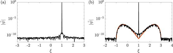
Figure 1: Spectral amplitude of the plane wave (4) with $\bar{\rho}=1$, $\overline{u}=1$ subject to the perturbation (12) with $\epsilon=10^{-11}$ after numerical evolution. (a) The defocusing case $\sigma=1$ at $t=20$, and $(b)$ the focusing case $\sigma=-1$ at $t=10$ with the predicted amplitude from linear theory in red.

Since the modulation equations (7) are elliptic when $\sigma=-1$, ill-posedness of the initial value problem for the modulation equations corresponds to MI of the Stokes wave [76]. Linearizing equations (7) about constant $\bar{\rho}$ and $\overline{u}$, we observe that the growth rate of perturbations $\propto e^{iK(X-\lambda_{1,2}T)}$ with wavenumber $K>0$ is $\mathrm{Im}\,\lambda_{2}K=\sqrt{\bar{\rho}}K$ when $\sigma=-1$. This coincides with the small $k$ expansion of the growth rate from the dispersion relation (11), $\mathrm{Im}\,\omega\sim\sqrt{\bar{\rho}}k$, $k\to 0$. Note that modulation theory does not predict a saturation of the growth rate, which, according to (11), occurs at the order one perturbation wavenumber $k=\sqrt{2\bar{\rho}}$.

The MI of the two-phase solution (9) can be determined by the hyperbolicity of the two-phase modulation equations (10). Since the modulation equations are hyperbolic (elliptic) when $\sigma=1$ ($\sigma=-1$), the two-phase solution is modulationally stable (unstable) and has been proven to be so by spectral analysis of the linearized operator when $\sigma=1$ [19] and $\sigma=-1$ [42, 29]. Furthermore, it has been shown that weak hyperbolicity of the modulation equations (all characteristic speeds are real) is a necessary condition for the modulational stability of nonlinear periodic wave trains [20, 48, 12]. Sufficiency is obtained when the modulation equations are strictly hyperbolic and the original PDE is Hamiltonian [49].

In Figure 2, we plot two numerical simulations of the perturbed two-phase solutions in the $\sigma=1$ case (Fig. 2(a,b)) at $t=150$ and the $\sigma=-1$ case (Fig. 2(c,d)) at $t=10$, respectively. Figures 2(a,c) depict the square modulus $|\psi|^{2}$ whereas Figs. 2(b,d) show the amplitude spectrum $|\widehat{\psi}|$. For these simulations, the carrier wavenumber is $\overline{u}=-0.5$ and the second phase wavenumber is $k=2$, and the amplitude parameter is $\bar{\rho}=1$. In both cases, there is a prominent peak at $\xi=\overline{u}$ in the amplitude spectrum with distinct harmonics at $\xi=\overline{u}+nk$, for integers $n$. In the stable case, $\sigma=1$, the spectrum is unchanged even for long time evolution.

The spectral features in Fig. 2(d) represent the early stage of MI, where the growth of the perturbation has not exceeded the largest spectral harmonics. The nonlinear stage of instability occurs for longer evolution times where the dynamics can be quite complicated, though the integrability of the NLS equation allows for the development of theory for both localized [17, 18] and random [41] perturbations.

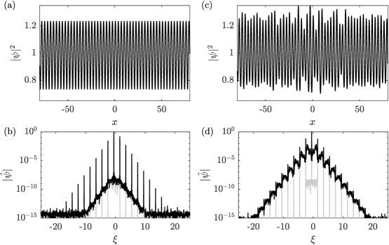
Figure 2: Initially perturbed two-phase solutions of the NLS equation with $\sigma=1$ at $t=150$ (a,b) and $\sigma=-1$ at $t=10$ (c,d). (a,c) depict the solution’s square modulus and (b,d) show the Fourier amplitude spectrum at the initial (gray) and final (black) times.

In the simplest cases presented here, Eq. (2) possesses both stable one-phase and two-phase solutions when $\sigma=1$ and both unstable one-phase and two-phase solutions when $\sigma=-1$. This motivates the following question. Does the addition of full dispersion into the NLS model (1) allow for situations in which one-phase, plane wave solutions are stable, but two-phase solutions with the same $\bar{\rho}$, $\overline{u}$ are unstable? After developing the modulation analysis, we will provide several physically inspired examples where the answer is yes.

1.3 Outline of this manuscript

This manuscript is organized as follows. In Sec. 2, we derive the Whitham modulation equations for two-phase wave trains in the FDNLS equation (1). In Sec. 3, we utilize the Whitham modulation equations to identify criteria for when both one-phase and two-phase wavetrains are stable with respect to long wave perturbations. We also obtain approximate two-phase solutions of the FDNLS equation with general $\Omega(k)$ for a plane wave subject to weakly nonlinear modulations in the second phase. Then, the corresponding two-phase Whitham modulation equations and their characteristic velocities are obtained in this regime. We identify an index that determines the modulation equation type and the different mechanisms that drive the instability of the underlying two-phase solution. In Sec. 4, we present phase diagrams predicting the stable/unstable two-phase solutions and the type of instability for several choices of dispersion $\Omega(k)$. These predictions are then compared with numerical simulations of perturbed two-phase solutions. Finally, in Sec. 5, we conclude with a discussion of the implications and extensions of the present theory.

2 Modulation theory for two-phase waves

The FDNLS equation (1) admits the one-phase, Stokes wave solutions

$$\psi(x,t)=\sqrt{\bar{\rho}}e^{i\theta_{1}},\quad\theta_{1}=\overline{u}x-\gamma t,\quad\gamma=\Omega(\overline{u})+f^{\prime}(\bar{\rho}),$$ (13)

for any $\bar{\rho}>0$ and $\overline{u}\in\mathbb{R}$. Here, $\overline{u}$ and $\gamma$ are the wavenumber, frequency pair, respectively. The solution (13) is referred to as the carrier wave. We assume the existence of a four-parameter family of two-phase solutions to Eq. (1) in the form

$$\psi(x,t)=\mathcal{U}(\theta_{2})e^{i\theta_{1}},\quad\theta_{1}=\overline{u}x-\gamma t,\quad\theta_{2}=kx-\omega t,$$ (14)

where $(\overline{u},\gamma)$ and $(k,\omega)$ are the first and second phase’s wavenumber and frequency, respectively. The oscillation periods for each phase are normalized to $2\pi$: $\psi(\theta_{1}+2\pi n,\theta_{2}+2\pi m)=\psi(\theta_{1},\theta_{2})$ for integers $n$, $m$. For incommensurate wavenumbers and frequencies, the solution (14) is quasi-periodic. Each of the frequencies $\gamma$ and $\omega$ generally depend on both wavenumbers $\overline{u}$ and $k$. The two-phase solution (14) can be parameterized, for example, in terms of the mean parameters

$$\bar{\rho}\equiv\frac{1}{4\pi^{2}}\int_{0}^{2\pi}\int_{0}^{2\pi}|\psi(\theta_{1},\theta_{2})|^{2}\,d\theta_{1}d\theta_{2},\quad\overline{u}\equiv\frac{i}{4\pi^{2}}\int_{0}^{2\pi}\int_{0}^{2\pi}(\psi_{x}^{*}\psi-\psi_{x}\psi^{*})/|\psi|^{2}\,d\theta_{1}d\theta_{2},$$ (15)

the wavenumber $k$, and amplitude $a$, which is the magnitude of the Fourier mode with wavenumber $\overline{u}+k$. The two-phase solution (14) is an amplitude and phase modulated Stokes waves (13). We demonstrate existence by obtaining approximate and numerical solutions in the weakly nonlinear regime.

Whitham modulation theory is a formal asymptotic procedure to derive a system of conservation laws that describe the slow evolution of a periodic or quasi-periodic solution [76, 37]. We now carry out the derivation of the modulation equations using Whitham’s original method of averaged conservation laws [74]. A modulated two-phase solution is sought in the form

$$\psi(x,t)=\mathcal{U}(\theta_{2},X,T)e^{i\theta_{1}}+\epsilon\psi_{1}(\theta_{1},\theta_{2},X,T)+\cdots,\quad\epsilon\to 0,$$ (16)

where $\theta_{1}$ is the carrier phase, $\theta_{2}$ is the second, envelope phase, and $\mathcal{U}$ is a complex modulation, which depends on $\theta_{2}$ and the slow scales $X=\epsilon x$, $T=\epsilon t$. The phase functions $\theta_{1},\theta_{2}$ are rapidly varying

$$\theta_{j}=S_{j}(X,T)/\epsilon~{},\quad j=1,2,$$

for smooth functions $S_{1}$, $S_{2}$. It is expedient to define the generalized wavenumbers and frequencies as

$$\begin{split}\theta_{1,x}&=S_{1,X}=\overline{u},\qquad\theta_{2,x}=S_{2,X}=k\\ \theta_{1,t}&=S_{1,T}=-\gamma,\qquad\theta_{2,t}=S_{2,T}=-\omega.\end{split}$$ (17)

The periods of $S_{1}$ and $S_{2}$ are fixed in order to ensure a well-ordered asymptotic expansion. Without loss of generality, we take these to be $2\pi$, so that $\mathcal{U}$ is also $2\pi$-periodic in $\theta_{2}$. Hence, $\mathcal{U}$ is represented by its Fourier series

$$\mathcal{U}(\theta_{2},X,T)=\sum_{n=-\infty}^{\infty}\widehat{q}_{n}(X,T)e^{in\theta_{2}}.$$ (18)

It is a straightforward calculation to prove that (1) possesses the following conserved quantities (14)

$$M[\psi] =\int|\psi|^{2}\ dx,$$ (19a)

$$P[\psi] =\int\left(\psi^{*}\psi_{x}-\psi\psi^{*}_{x}\right)\ dx,$$ (19b)

$$E[\psi] =\int\big{(}\psi^{*}\Omega(-i\partial_{x})\psi+f(|\psi|^{2})\big{)}dx,$$ (19c)

corresponding respectively to mass, momentum, and energy.

Two modulation equations are found by inserting the multiple scales expansion (16) into the first two conservation laws corresponding to $M$ and $P$ integrated over the two-phase solution family. Replacing partial derivatives in $x,t$ with appropriate partial derivatives in $\theta_{1},\theta_{2},X$, and $T$, the linear dispersion operator $\Omega$ is expanded in a similar way to the expansions of the dispersion operators in the scalar Whitham equation [14]. We extend those results to the case where the operator is acting on a function of two independent phase variables and obtain, to $\mathcal{O}(\epsilon)$, that

$$\begin{split}\widetilde{\Omega}(-i\partial_{x})\psi(x,t)&=\widetilde{\Omega}(D-i\epsilon\partial_{X})\psi(\theta_{1},\theta_{2},X,T)\\ &=\widetilde{\Omega}(D)\psi+i\frac{\epsilon}{2}\left[\widetilde{\Omega}^{\prime}(D)\psi_{X}+\left(\widetilde{\Omega}^{\prime}(D)\psi\right)_{X}\right]+\mathcal{O}(\epsilon^{2})~{},\end{split}$$ (20)

where $D=-i\partial_{\theta_{1}}-i\partial_{\theta_{2}}$, and $\widetilde{\Omega}^{\prime}(\cdot)$ is the pseudo-differential operator corresponding to the symbol $\Omega^{\prime}(\xi)$. The proof for single-phase functions can be found in the appendix of Ref. [14], where $\Omega(\xi)$ is assumed to be analytic. However, this requirement can be relaxed to three weak derivatives of $\Omega(k)$ in an appropriate function space [22].

We now outline the derivation of the modulation equation that is a consequence of mass conservation (19a). First, one expands the conserved quantity (19a)

$$\begin{split}\frac{d}{dt}\int_{0}^{2\pi}\!\!\!\int_{0}^{2\pi}|\psi|^{2}\ d\theta_{1}d\theta_{2}=\!\!\int_{0}^{2\pi}\!\!\!\int_{0}^{2\pi}(-\gamma\partial_{\theta_{1}}-\omega\partial_{\theta_{2}}+\epsilon\partial_{T})|\psi|^{2}\ d\theta_{1}d\theta_{2}=\epsilon\left(\overline{|\mathcal{U}|^{2}}\right)_{T}+\mathcal{O}(\epsilon^{2}),\end{split}$$ (21)

where the averaging operator is denoted

$$\overline{F[\psi]}(X,T)=\int_{0}^{2\pi}\int_{0}^{2\pi}F[\psi(\theta_{1},\theta_{2},X,T)]\,d\theta_{1}d\theta_{2}.$$

We now determine the representation of the averaged mass flux. This can be achieved by alternatively replacing $t$-derivatives of $\psi$ with the right hand side of Eq. (1) and uses (18) to find that

$$\begin{split}\frac{d}{dt}\int_{0}^{2\pi}\int_{0}^{2\pi}|\psi|^{2}\ d\theta_{1}d\theta_{2}&=-\epsilon\left(\sum_{n}\Omega^{\prime}(\overline{u}+nk)|q_{n}|^{2}\right)_{X}+\mathcal{O}(\epsilon^{2}).\end{split}$$ (22)

Equating terms at $\mathcal{O}(\epsilon)$ from (21) and (22) results in averaged mass conservation

$$\left(\overline{|\mathcal{U}|^{2}}\right)_{T}+\left(\sum_{n}\Omega^{\prime}(\overline{u}+nk)|q_{n}|^{2}\right)_{X}=0.$$ (23)

Similar calculations with (19b) and (19c), yield averaged momentum conservation

$$\begin{split}&\left(\sum_{n}(\overline{u}+nk)|q_{n}|^{2}\right)_{T}+\left(\overline{f^{\prime}(|\mathcal{U}|^{2})|\mathcal{U}|^{2}-f(|\mathcal{U}|^{2})}\right)_{X}\\ &\qquad\qquad\qquad\qquad~{}\,+\left(\sum_{n}(\overline{u}+nk)\Omega^{\prime}(\overline{u}+nk)|q_{n}|^{2}\right)_{X}=0,\end{split}$$ (24)

and averaged energy conservation

$$\begin{split}&\left(\overline{\mathcal{U}^{*}\widetilde{\Omega}(D)\mathcal{U}+f(|\mathcal{U}|^{2})}\right)_{T}+\left(\sum_{n}\Omega(\overline{u}+nk)\Omega’(\overline{u}+nk)|q_{n}|^{2}\right)_{X}\\ &\quad+\frac{1}{2}\left(\overline{\mathcal{U}^{*}\left(\widetilde{\Omega}’(D)f’(|\mathcal{U}|^{2})\mathcal{U}\right)+f’(|\mathcal{U}|^{2})\mathcal{U}\left(\widetilde{\Omega}’(D)\mathcal{U}^{*}\right)}\right)_{X}=0.\end{split}$$ (25)

Two additional modulation equations are obtained by requiring that the phase variables are twice continuously differentiable, i.e., $S_{j,XT}=S_{j,TX}$ for $j=1,2$. These constraints result in the two conservation of waves equations

$$\overline{u}_{T}+\gamma_{X} =0,$$ (26a)

$$k_{T}+\omega_{X} =0.$$ (26b)

Equations (23), (24), (25), (26a), and (26b) are five conservation laws for the four dependent variables $(\bar{\rho},\overline{u},k,a)$. The averaged energy equation is, generically, redundant with the remaining four modulation equations [76, 11]. We will focus on the averaged mass (23), averaged momentum (24), and conservation of waves equations (26a), (26b) as a closed set of modulation equations for the four modulation parameters $(\bar{\rho},\overline{u},k,a)$. In what follows, we study properties of these equations with increasing levels of complexity.

3 Modulations of one- and two-phase wavetrains

3.1 One-phase modulations

The modulation equations for the one-phase Stokes wave $\psi=\sqrt{\bar{\rho}}e^{i\theta_{1}}$ can be obtained from the two-phase modulation equations by taking $q_{n}\to 0$ for $n\neq 0$ where $q_{0}=\sqrt{\bar{\rho}}$. Then, Eqs. (23) and (26a) become

$$(\bar{\rho})_{T}+\left(\bar{\rho}\Omega^{\prime}(\overline{u})\right)_{X} =0$$ (27a)

$$\overline{u}_{T}+(f^{\prime}(\bar{\rho})+\Omega(\overline{u}))_{X} =0,$$ (27b)

When $q_{n}=0$, $n\neq 0$, the momentum and energy conservation laws (24), (25) are an immediate consequence of (27). The remaining modulation equation (26b) limits to

$$k_{T}+\left(\omega_{0}^{(\pm)}\right)_{X}=0,$$ (28)

where $\omega_{0}^{(\pm)}$ is the linear dispersion relation of the FDNLS equation (1) for waves propagating on the Stokes wave

$$\begin{split}\omega_{0}^{(\pm)}&=\mathcal{N}_{1}\pm\sqrt{\mathcal{M}_{1}(\mathcal{M}_{1}+2\bar{\rho}f^{\prime\prime}(\bar{\rho}))},\\ \mathcal{N}_{1}&=\tfrac{1}{2}(\Omega(\overline{u}+k)-\Omega(\overline{u}-k)),\quad\mathcal{M}_{1}=\tfrac{1}{2}\left(\Omega(\overline{u}+k)-2\Omega(\overline{u})+\Omega(\overline{u}-k)\right).\end{split}$$ (29)

The dispersionless modulation equations (27) are a $2\times 2$ system of conservation laws for the variables $(\bar{\rho},\overline{u})$ that are independent of $k$. We therefore first consider the evolution of $(\bar{\rho},\overline{u})$ according to (27) and then discuss the evolution of $k$ in (28).

Equations (27) exhibit the characteristic velocities

$$\lambda_{1,2}=\Omega^{\prime}(\overline{u})\pm\sqrt{\bar{\rho}f^{\prime\prime}(\bar{\rho})\Omega^{\prime\prime}(\overline{u})}~{},$$ (30)

which are real and strictly ordered $\lambda_{1}<\lambda_{2}$ if and only if

$$\bar{\rho}f^{\prime\prime}(\bar{\rho})\Omega^{\prime\prime}(\overline{u})>0~{}.$$

In this case, the modulation equations (27) are strictly hyperbolic. Equations (27) are diagonalized in terms of the Riemann invariants

$$r_{1,2}=\int^{\overline{u}}\sqrt{\Omega^{\prime\prime}(\tau)}d\tau\pm\int^{\bar{\rho}}\sqrt{\frac{f^{\prime\prime}(s)}{s}}ds,$$

so that Eqs. (27) are equivalent to $r_{j,T}+\lambda_{j}r_{j,X}=0$, $j=1,2$. The system (27) is genuinely nonlinear so long as $\nabla\lambda\cdot\mathbf{r}\neq 0$ for each eigenvalue-eigenvector pair $(\lambda,\mathbf{r})$ [56]. For cubic nonlinearity, $f^{\prime}(\bar{\rho})=\bar{\rho}$, the loss of genuine nonlinearity occurs when $3\Omega^{\prime\prime}(\overline{u})^{3/2}=\pm\sqrt{\bar{\rho}}\Omega^{\prime\prime\prime}(\overline{u})$.

The classical MI criterion

$$\bar{\rho}f^{\prime\prime}(\bar{\rho})\Omega^{\prime\prime}(\overline{u})<0~{},$$ (31)

is obtained when the velocities (30) are complex. We define the carrier-phase MI index

$$\Delta_{\rm CPMI} =\mathrm{sgn}\left[\bar{\rho}f^{\prime\prime}(\bar{\rho})\Omega^{\prime\prime}(\overline{u})\right]~{},$$ (32)

so that the condition for classical MI is $\Delta_{\rm CPMI}=-1$ [76]. This criterion is equivalent to $\sigma=-1$ in the NLS equation (2) for modulations of a Stokes wave in dispersive, nonlinear media [14].

The conservation of waves (28) describes the evolution of infinitesimal (linear) waves propagating on a modulated Stokes wave. Its characteristic velocity is the group velocity $\omega^{(\pm)}_{0,k}(k,\bar{\rho},\overline{u})$ whose long wavelength limit $\lim_{k\to 0}\omega^{(\pm)}_{0,k}=\lambda_{1,2}$ coincides with one of Eq. (30). When $\Delta_{\rm CPMI}=-1$, the instability’s growth rate in the linear regime is $\mathrm{Im}\,\omega^{(\pm)}_{0}$. This linearization of the FDNLS equation about the Stokes wave (13) and subsequent analysis was previously identified as the extended criterion for modulational instability [5]. In what follows, we investigate the scenario when the Stokes wave is modulationally stable according to the extended MI criterion $\Delta_{\rm CPMI}=1$ but exhibits an instability due to finite amplitude modulations involving a second phase.

3.2 Weakly nonlinear, two-phase wavetrains

To approximate the two-phase solution, we insert (14) into (1) and obtain

$$(-\gamma+i\omega{\partial_{\theta_{2}}})\mathcal{U} =\widetilde{\Omega}\left(\overline{u}-ik{\partial_{\theta_{2}}}\right)\mathcal{U}\ +\ f^{\prime}(|\mathcal{U}|^{2})\mathcal{U}~{}.$$ (33)

Introducing the small amplitude parameter $0<a\ll 1$, expanding the solution as

$$\begin{split}\mathcal{U}&=\sqrt{\rho_{0}}+ae^{i\theta_{2}}+aB_{1}e^{-i\theta_{2}}+a^{2}A_{2}e^{2i\theta_{2}}+a^{2}B_{2}e^{-2i\theta_{2}}+\ldots,\\ \gamma&=\gamma_{0}\ +\ a^{2}\gamma_{2}\ +\ \ldots\qquad\omega=\omega_{0}\ +\ a^{2}\omega_{2}\ +\ \ldots,\end{split}$$ (34)

inserting the expansions into (33), and gathering terms in powers of $a$, we solve the resulting linear problems for $A_{2}$, $B_{j}$, $\gamma_{j}$, $\omega_{j}$ for $j=1,2$. The results of the perturbation analysis up to $\mathcal{O}(a^{2})$ are

$$\begin{split}\gamma_{0}&=f^{\prime}(\rho_{0})+\Omega(\overline{u}),\quad\omega_{0}^{(\pm)}=\mathcal{N}_{1}\pm\sqrt{\mathcal{P}},\quad B_{1}^{(\pm)}=-1+\frac{\mathcal{M}_{1}\pm\sqrt{\mathcal{P}}}{\rho_{0}f^{\prime\prime}(\rho_{0})},\\[5.69054pt] A_{2}^{(\pm)}&=\frac{\sqrt{\rho_{0}}}{\mathcal{D}}\left[(\mathcal{M}_{2}-\mathcal{N}_{2}+2\gamma_{0})\left(\mathcal{G}^{(\pm)}_{3}+2(2B_{1}^{(\pm)}+1)f^{\prime\prime}(\rho_{0})\right)-\mathcal{G}^{(\pm)}_{2}\right],\\[5.69054pt] B_{2}^{(\pm)}&=-\frac{\sqrt{\rho_{0}}}{\mathcal{D}}\left[(\mathcal{M}_{2}+\mathcal{N}_{2}-2\gamma_{0})\left(\mathcal{G}^{(\pm)}_{3}+2B_{1}^{(\pm)}(B_{1}^{(\pm)}+2)f^{\prime\prime}(\rho_{0})\right)-\mathcal{G}^{(\pm)}_{2}\right],\\[5.69054pt] \gamma_{2}^{(\pm)}&=2\left(\left(B_{1}^{(\pm)}\right)^{2}+B_{1}^{(\pm)}+1\right)f^{\prime\prime}(\rho_{0})+\mathcal{G}^{(\pm)}_{3},\end{split}$$ (35a)

and

$$\begin{split}\omega_{2}^{(\pm)}&=\frac{1}{2((B_{1}^{(\pm)})^{2}-1)}\bigg{[}2\left((1+2B_{1}^{(\pm)})A_{2}^{(\pm)}+B_{1}^{(\pm)}(2+B_{1}^{(\pm)})B_{2}^{(\pm)}\right)\\ &\quad\times\left((B_{1}^{(\pm)})^{4}+2(B_{1}^{(\pm)})^{3}+2B_{1}^{(\pm)}+1-2\sqrt{\rho_{0}}f^{\prime\prime}(\rho_{0})\right)\\ &\quad-\left(\sqrt{\rho_{0}}(A_{2}^{(\pm)}+B_{2}^{(\pm)})+(1+(B_{1}^{(\pm)})^{2})\right)\mathcal{G}^{(\pm)}_{3}+\rho_{0}f^{(4)}(\rho_{0})(1+B_{1}^{(\pm)})^{4}\bigg{]},\end{split}$$ (35b)

where we introduce

$$\mathcal{M}_{j} =\tfrac{1}{2}\left(\Omega(\overline{u}+jk)-2\Omega(\overline{u})+\Omega(\overline{u}-jk)\right),\quad\mathcal{N}_{j}=\tfrac{1}{2}\left(\Omega(\overline{u}+jk)-\Omega(\overline{u}-jk)\right),$$

$$\mathcal{P} =\mathcal{M}_{1}\left(\mathcal{M}_{1}+2\rho_{0}f^{\prime\prime}(\rho_{0})\right)~{},\quad\mathcal{G}^{(\pm)}_{2}=2\left(B_{1}^{2}-1\right)\rho_{0}[f^{\prime\prime}(\rho_{0})]^{2},$$ (35c)

$$\mathcal{G}^{(\pm)}_{3} =(B_{1}+1)^{2}\rho_{0}f^{(3)}(\rho_{0}),\quad\mathcal{D}=2(2\gamma_{0}-\mathcal{N}_{2})^{2}-\mathcal{M}_{2}\left(\mathcal{M}_{2}+2\rho_{0}f^{\prime\prime}(\rho_{0})\right).$$

The approximate two-phase solution is given by (34) and (35). A few remarks are in order. There are two solutions for $\omega_{0}^{(\pm)}$ as in (29). Hence, there are two distinct branches of two-phase solutions bifurcating from the one-phase solution. The denominator of $\omega_{2}^{(\pm)}$ in (35b) is zero when $|B_{1}^{(\pm)}|=1$. This occurs only when $\mathcal{M}_{1}=0$ or $\rho_{0}=0$, which we exclude from further consideration. In general, $\mathcal{M}_{j}$ and $\mathcal{N}_{j}$ depend on both $\overline{u}$ and $k$, and hence so do $\omega_{0}^{(\pm)},\gamma_{2}$, and $\omega_{2}^{(\pm)}$. The terms $\mathcal{M}_{j}$ and $\mathcal{N}_{j}$ are the discrete Laplacian and centered difference, respectively, that capture the dispersion’s nonlocality with the long wavelength limits $\mathcal{M}_{j}\sim\frac{1}{2}(jk)^{2}\Omega^{\prime\prime}(\overline{u})$, $\mathcal{N}_{j}\sim\frac{1}{2}jk\Omega^{\prime}(\overline{u})$ as $k\to 0$.

3.3 Modulation system for weakly nonlinear two-phase solutions

Inserting the two-phase solution (34)–(35) into the modulation system for mass (23), momentum (24), and conservation of waves (26a), (26b) while retaining terms up to $\mathcal{O}(a^{2})$, we arrive at

$$\left(\rho_{0}+a^{2}(B_{1}^{2}+1)\right)_{T}+\left(\rho_{0}\Omega^{\prime}(\overline{u})+a^{2}\mathcal{Q}_{+}\right)_{X} =0~{},$$ (36a)

$$\begin{split}\left(\rho_{0}\overline{u}+a^{2}(\overline{u}+k+B_{1}^{2}(\overline{u}-k))\right)_{T}\hskip 137.31255pt\\[5.69054pt] +\left[-f(\rho_{0})+\rho_{0}\left(f^{\prime}(\rho_{0})+\overline{u}\Omega^{\prime}(\overline{u})\right)+a^{2}\left(\rho_{0}\gamma_{2}+\overline{u}\mathcal{Q}_{+}+k\mathcal{Q}_{-}\right)\right]_{X}&=0~{},\end{split}$$ (36b)

$$\overline{u}_{T}+(\gamma_{0}+a^{2}\gamma_{2})_{X} =0~{},$$ (36c)

$$k_{T}+(\omega_{0}+a^{2}\omega_{2})_{X} =0~{},$$ (36d)

where we introduce

$$\mathcal{Q}_{\pm} =\Omega^{\prime}(\overline{u}+k)\pm B_{1}^{2}\Omega^{\prime}(\overline{u}-k),$$ (37)

and have suppressed the superscript ^(±) denoting the fast ($+$)/slow ($-$) branch of two-phase solutions—which differs from the subscript in $\mathcal{Q}_{\pm}$—for ease of presentation. Note that $\mathcal{Q}_{\pm}$ depend also on $\rho_{0}$ via $B_{1}$ (35a).

3.4 Characteristic velocities of the weakly nonlinear modulation system

To compute the characteristic velocities $\{\lambda_{j}\}_{j=1}^{4}$ of the Whitham modulation equations (36), we can cast them in the quasilinear form

$$\mathcal{A}\mathbf{q}_{T}+\mathcal{B}\mathbf{q}_{X}=0,\qquad\mathbf{q}=\left[\rho_{0},\overline{u},a^{2},k\right]^{\rm T}$$ (38)

and solve the generalized eigenvalue problem $\mathcal{B}\mathbf{v}=\lambda\mathcal{A}\mathbf{v}$. We compute the eigenvalues perturbatively in the amplitude parameter $a$. At leading order, the eigenvalues are

$$\lambda_{1,2} =\Omega^{\prime}(\overline{u})\pm\sqrt{\rho_{0}f^{\prime\prime}(\rho_{0})\Omega^{\prime\prime}(\overline{u})}~{},$$ (39)

$$\lambda_{3} =\lambda_{4}=\frac{\partial\omega_{0}}{\partial k}~{}.$$ (40)

Here, $\lambda_{1,2}$ are simple eigenvalues for the mean variables $\bar{\rho}=\rho_{0}+\mathcal{O}(a^{2})$ and $\overline{u}$ (the same as in (30)). The double eigenvalue is degenerate, with geometric multiplicity one. Then, $\mathcal{O}(a^{2})$ perturbation of the eigenvalue problem will lead to $\mathcal{O}(a^{2})$ corrections to $\lambda_{1,2}$ and an $\mathcal{O}(a)$ bifurcation of the double eigenvalue $\lambda_{3}=\lambda_{4}$. We are interested in the $\mathcal{O}(a)$ bifurcation of the double eigenvalue. Consequently, we can avoid a full perturbative analysis of the $4\times 4$ eigenvalue problem in favor of a simpler, more direct approach that utilizes the structure of the modulation equations themselves. That is, we assume that the variations in the mean $(\bar{\rho},\overline{u})$ are induced solely by the finite amplitude wave while the leading order mean is taken to be constant [76, 35]. We make the ansatz

$$\rho_{0} =R_{0}+a^{2}R_{2}(k),\quad\overline{u}=U_{0}+a^{2}U_{2}(k),$$ (41)

where $(R_{0},U_{0})$ is the constant background and $(R_{2},U_{2})$ is the induced mean. The latter can be determined by inserting (41) into (36a) and (36c), and recalling (35) and (37). The leading order terms vanish, while the $\mathcal{O}(a^{2})$ terms yield

$$\left(R_{2}+1+B_{1}^{2}\right)_{T}+\left(\Omega^{\prime}(U_{0})R_{2}+\Omega^{\prime\prime}(U_{0})R_{0}U_{2}+\mathcal{Q}_{+,0}\right)_{X} =0~{},$$ (42a)

$$U_{2,T}+\left(f^{\prime\prime}(R_{0})R_{2}+\Omega^{\prime}(U_{0})U_{2}+\gamma_{2}\right)_{X} =0~{},$$ (42b)

where $\mathcal{Q}_{+,0}=\mathcal{Q}_{+}(R_{0},U_{0})$.

As a consequence of the conservation of waves (26b), for any differentiable function $F(k(X,T))$, the conservation law

$$\left(F(k)\right)_{T}+\left(\omega_{0,k}F(k)\right)_{X}=0$$ (43)

is satisfied. Comparing (41)–(43) with $F=R_{2}+1+B$ and $F=U_{2}$, we arrive at the algebraic system for the induced mean

$$\begin{bmatrix}\Omega^{\prime}(U_{0})-\omega_{0,k}&\Omega^{\prime\prime}(U_{0})R_{0}\\ f^{\prime\prime}(R_{0})&\Omega^{\prime}(U_{0})-\omega_{0,k}\end{bmatrix}\begin{bmatrix}R_{2}\\ U_{2}\end{bmatrix}=\begin{bmatrix}\omega_{0,k}(1+B_{1}^{2})-\mathcal{Q}_{+,0}\\ -\gamma_{2}\end{bmatrix},$$

whose solution is

$$\begin{bmatrix}R_{2}\\ U_{2}\end{bmatrix} =\frac{1}{\Delta}\begin{bmatrix}\left(\omega_{0,k}-\Omega^{\prime}(U_{0})\right)\left(\mathcal{Q}_{+,0}-(1+B_{1}^{2})\right)+\Omega^{\prime\prime}(U_{0})R_{0}\gamma_{2}\\[5.69054pt] \left(\omega_{0,k}-\Omega^{\prime}(U_{0})\right)\gamma_{2}-f^{\prime\prime}(R_{0})\left(\mathcal{Q}_{+,0}-(1+B_{1}^{2})\right)\end{bmatrix},$$ (44)

with determinant

$$\Delta =\left(\omega_{0,k}-\Omega^{\prime}(U_{0})\right)^{2}-R_{0}f^{\prime\prime}(R_{0})\Omega^{\prime\prime}(U_{0})~{}.$$ (45)

The nonlinear frequency shift is obtained by expanding

$$\omega_{0}(R_{0}+a^{2}R_{2},U_{0}+a^{2}U_{2}) =\omega_{0}(R_{0},U_{0})+a^{2}\tilde{\omega}_{2}+\mathcal{O}(a^{4}),$$

where

$$\tilde{\omega}_{2}(k) =\omega_{2}(R_{0},U_{0})+\left[R_{2}(k),U_{2}(k)\right]\cdot\left.\nabla_{\rho_{0},\overline{u}}\omega_{0}\right|_{\rho_{0}=R_{0},\overline{u}=U_{0}},$$ (46)

and $\omega_{2}$ is given in eq. (35b). Incorporating the nonlinear frequency shift (46) into the modulation equations (36a) and (36d) results in the modulation system

$$a_{T}+\omega_{0,k}a_{X}+\tfrac{1}{2}\omega_{0,kk}ak_{X}=0,\quad k_{T}+\omega_{0,k}k_{X}+2a\tilde{\omega}_{2}(k)a_{X}=0.$$ (47)

The characteristic velocities of (47) include the sought for perturbations of the degenerate, double eigenvalue (40). Then, the characteristic velocities of the weakly nonlinear modulation system (36) are

$$\lambda_{1,2} =\Omega^{\prime}(\overline{u})\pm\sqrt{\rho_{0}f^{\prime\prime}(\rho_{0})\Omega^{\prime\prime}(\overline{u})}+\mathcal{O}(a^{2})~{},$$ (48a)

$$\lambda_{3,4} =\omega_{0,k}\pm a\sqrt{\omega_{0,kk}\tilde{\omega}_{2}}+\mathcal{O}(a^{2})~{}.$$ (48b)

3.5 Generalized MI for small amplitude two-phase wavetrains

For the basis of this discussion, we assume that the dispersionless system is hyperbolic, i.e., $\lambda_{1,2}$ are real. We further assume that the two-phase wavetrain, in the harmonic limit does not experience exponential growth or decay, meaning that $\omega_{0}$ is real valued. Under these assumptions, the only mechanism that remains to change the type of the modulation equations is a change of the second-phase MI index

$$\Delta_{\rm SPMI}=\mathrm{sgn}\left(\omega_{0,kk}\tilde{\omega}_{2}\right)~{}.$$ (49)

This index provides a generalized criterion for MI of two-phase waves. When $\Delta_{\rm SPMI}=1$, the characteristic velocities $\lambda_{3,4}$ are real. When $\Delta_{\rm CPMI}=\Delta_{\rm SPMI}=1$, the modulation system (36) is hyperbolic. When $\Delta_{\rm SPMI}=-1$, $\lambda_{3,4}$ are complex valued and, if $\Delta_{\rm CPMI}=1$, the modulation equations are of mixed hyperbolic-elliptic type.

By examining $\Delta_{\rm SPMI}$, we can identify potential mechanisms for a change in type of the modulation system when $\omega_{0,kk}\tilde{\omega}_{2}$ is zero or singular. These include:

• zero linear dispersion curvature: $\omega_{0,kk}=0$;

• four-wave mixing: $\omega_{0,kk}\to\infty$ when $\Omega(\overline{u}+2k)-2\Omega(\overline{u})+\Omega(\overline{u}-2k)=0$ ($\mathcal{M}_{2}=0$);

• short-long wave resonance: $\Delta=0$ in (44) and (45) when $\omega_{0,k}=\Omega^{\prime}(\overline{u})\pm\sqrt{\bar{\rho}_{0}f^{\prime\prime}(\bar{\rho})\Omega^{\prime\prime}(\overline{u})}$;

• second harmonic resonance: $A_{2}$, $B_{2}\to\infty$ in (34) when $2\omega_{0}(k,\bar{\rho},\overline{u})=\omega_{0}(2k,\bar{\rho},\overline{u})$ ($\mathcal{D}=0$ in (35));

• other nonlinear mechanisms: $\tilde{\omega}_{2}=0$.

4 Examples

In this section, we analyze the second-phase index $\Delta_{\rm SPMI}$ (49) for some specific FDNLS equations as a way to predict the onset of instability. The FDNLS equation (1) is considered with cubic nonlinearity $f^{\prime}(|\psi|^{2})=|\psi|^{2}$ and four distinct dispersion relations $\Omega(k)$ corresponding to third and fourth-order dispersion as well as finite-depth water waves and discrete nonlinear lattices. Without loss of generality, we consider normalized two-phase solutions (14) with $\bar{\rho}=\overline{|\mathcal{U}|^{2}}=1$. Since our objective is to identify instabilities using $\Delta_{\rm SPMI}$, we only consider modulationally stable one-phase carrier wavenumbers $\overline{u}$ for which $\Delta_{\rm CPMI}=1$ (32).

In Secs. 4.1 and 4.2, we numerically compute two-phase solutions of the FDNLS equation (1) of the form (14) by solving the nonlinear eigenvalue problem

$$-i\omega\mathcal{U}+\gamma\mathcal{U}_{\theta_{2}}=|\mathcal{U}|^{2}\mathcal{U}+\Omega(\overline{u}-ik\partial_{\theta_{2}})\mathcal{U},$$ (50)

using an iterative Newton-conjugate gradient algorithm for the Fourier coefficients of $\mathcal{U}$ [77, 78], initialized with the weakly nonlinear approximation (34). Direct simulations of the FDNLS equation (1) are then performed using a fourth-order split-step scheme [79] with initial condition the two-phase solution perturbed with small additive noise (12) with wavenumbers in the band $\xi\in(\overline{u}-k,\overline{u}+k)$, similar to the numerical simulations of perturbed solutions in Sec. 1.2.

4.1 NLS with third-order dispersion

The cubic NLS equation with third-order dispersion (NLS3) is

$$i\psi_{t}=\frac{i}{6}\psi_{xxx}+|\psi|^{2}\psi.$$ (51)

The linear dispersion relation is

$$\left(\omega_{0}-\frac{1}{2}\overline{u}^{2}k-\frac{k^{3}}{6}\right)^{2}=\overline{u}k^{2}\left(4+\overline{u}k^{2}\right)~{}.$$ (52)

When $\overline{u}\geq 0\,$, $\omega_{0}^{(\pm)}\in\mathbb{R}$ so that the one-phase solution (13) is modulationally stable. The two branches of the dispersion relation correspond to the phase velocities $c_{\pm}(k)=\omega_{0}^{(\pm)}(k)/k$ subject to inter-branch ($c_{+}(k_{1})=c_{-}(k_{2})$) and intra-branch ($c_{+}(k_{1})=c_{+}(k_{2})$) linear resonances. Despite being linear resonances, they can be induced by nonlinearity, as demonstrated below. Figures 3(a) and 3(b) depict inter- and intra-branch resonances, respectively.

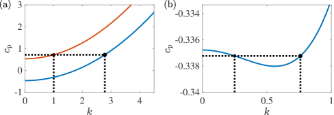
Figure 3: Example linear resonances for the NLS3 equation (51): (a) inter-branch resonance $c_{+}(k_{1})=c_{-}(k_{2})$ of the fast $k_{1}=1$ (red) and slow $k_{2}\approx 2.789$ (blue) dispersion branches for $\overline{u}=0.25$; (b) intra-branch resonance $c_{-}(k_{1})=c_{-}(k_{2})$ for $k_{1}=0.25$, $k_{2}\approx 0.76$, $\overline{u}=1.5$.

We evaluate $\Delta_{\rm SPMI}$ (49) for Eq. (51) and plot the results in Fig. 4(a,b). The grayscale colormap depicts the imaginary part of the Whitham velocities (48) $\mathrm{Im}(\sqrt{\tilde{\omega_{2}}\omega_{0,kk}})$ on a log scale, taken as a quantitative measure of the strength of the instability, on the order of the exponential growth rate. Figures 4(a) and (b) depict $\Delta_{\rm SPMI}$ for the fast ⁽⁺⁾ and slow ^(-) branches, respectively, of two-phase solutions (34) as a function of $\overline{u}$ and $k$. Grayscale regions correspond to negative index $\Delta_{\rm SPMI}=-1$ and unstable two-phase solutions. White regions correspond to positive index $\Delta_{\rm SPMI}=1$. The pink regions in Fig. 4(a) indicate the existence of either an inter- or intra-branch resonant wave with $\Delta_{\rm SPMI}=-1$.

In Figures 4(a,b), 5(a,b), 6, and 7 depicting $\Delta_{\rm SPMI}$, the solid curves identify one of the instability mechanisms listed in Sec. 3.5. An orange curve identifies a short-long wave resonance. Blue denotes a second-harmonic resonance. Green indicates zero-dispersion curvature whereas black connotes other nonlinear mechanisms. In this example there are no changes in sign of the $\Delta_{\rm SPMI}$ due to 4-wave mixing. Figure 4(a) predicts that the fast two-phase solution (34) is unstable for all wavenumber pairs $(\overline{u},k)$ due to either second-harmonic resonance, other nonlinear mechanisms, or the secondary instability of a linearly resonant mode. Figure 4(b) predicts bands of unstable, slow two-phase solutions due to all available mechanisms.

To test the accuracy of our predictions, we compare them to the numerical evolution of Eq. (51) for several computed two-phase solutions. Figure 4(c) shows the wave power $|\psi(x,t)|^{2}$ and magnitude of the Fourier transform $|\widehat{\psi}(\xi,t)|$ at time $t=2500$ corresponding to the perturbed, fast two-phase solution with $(\overline{u},k)=(\pi/10,\pi/3)$ and $a=0.05$ identified in Fig. 4(a). For these parameters, there is an inter-branch resonant mode with wavenumber $k_{\rm res}\approx 2.789$. Since the slow two-phase solution with $(\overline{u},k)=(\pi/10,k_{\rm res})$ is predicted to be unstable, we can interpret the small amplitude, shorter wavelength modulations of $|\psi|^{2}$ as caused by the slow growth of a resonant mode. Indeed, the Fourier spectrum at $t=2500$ shows a peak at $k\approx\overline{u}+k_{\rm res}$ indicated by the red line that was not in the initial data (gray).

Figure 4(d) shows an example of an unstable mode at $t=1500$. In the long time evolution, modulations of $|\psi|^{2}$ are visible in Fig. 4(d) due to the two-phase instability. The spectrum reveals the emergent side-bands, which are indicated by the peaks at $\overline{u}+nk$ for $n\in\mathbb{Z}$.

Figure 4(e) is an example of an instability arising due to a longer wave intra-branch resonance. We evolve a perturbed, slow two-phase solution with $(\overline{u},k)=(\pi/2,8\pi/11)$ and $a=0.001$ to $t=1000$. There is an intra-branch resonant mode at $k_{\rm res}\approx 1.078$. In this case, the initial two-phase solution is predicted to be stable, while the resonant mode is predicted to be unstable. The power in Fig. 4(e) exhibits strong modulations with wavelength longer than $2\pi/k=11/4$. The spectrum reveals wide bands centered at $\overline{u}+k_{\rm res}$ and its harmonics. These bands’ ampltiude grows with time. Despite this growth, the spectral peaks of the initial two-phase solution remain relatively unchanged on the time scale of the numerical experiment.

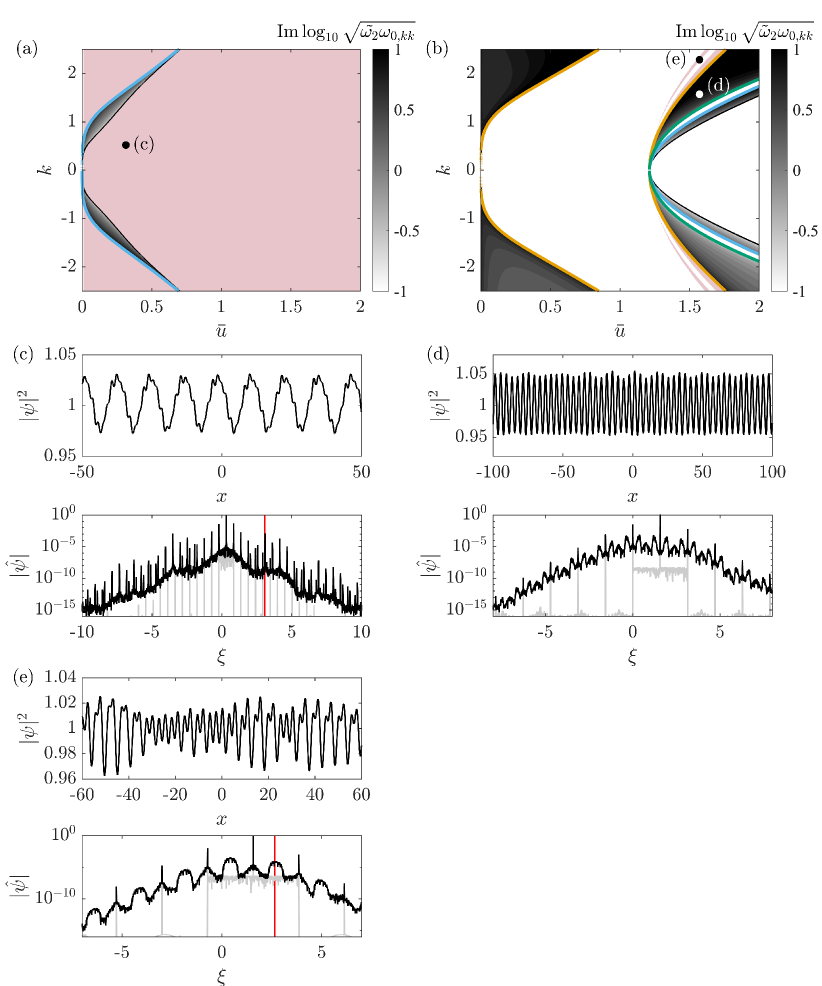
Figure 4: Phase diagrams indicating the stability (white) or instability (grayscale) of small-amplitude, fast (a) and slow (b) two-phase solutions of the NLS3 equation (51). The grayscale indicates the predicted strength of the instability. Pink regions indicate the presence of an unstable resonant mode. (c)-(e) present the results of direct numerical simulations of the NLS3 equation. The upper (lower) panels show the power $|\psi(x,t)|^{2}$ (spectral intensity $|\widehat{\psi}(k,t)|$) in black after time integration. The initial spectrum $|\widehat{\psi}(k,0)|$ is shown in gray. Red lines identify $\overline{u}+k_{\rm res}$.

4.2 NLS with fourth-order dispersion

Consider the cubic NLS equation with fourth-order dispersion (NLS4)

$$i\psi_{t}=\frac{1}{24}\psi_{xxxx}+|\psi|^{2}\psi~{}.$$ (53)

This equation exhibits no classical MI since $\Delta_{\rm CPMI}=1$ in (32). The linear dispersion relation $\omega_{0}$ satisfies

$$\left(6\omega_{0}-\overline{u}k(\overline{u}^{2}+k^{2})\right)^{2}=\frac{1}{16}k^{2}\left(k^{2}+6\overline{u}^{2}\right)\left(k^{4}+6k^{2}\overline{u}^{2}+48\right),$$ (54)

so that $\omega_{0}$ is real-valued for all $\overline{u},k\in\mathbb{R}$.

Figures 5(a) and (b) depict the stability of fast and slow, respectively, weakly nonlinear two-phase solutions according to $\Delta_{\rm SPMI}$. We focus on the gray islands bounded by the black curves. These regions are particularly notable since their boundaries correspond to sign changes in the modified nonlinear frequency shift, $\tilde{\omega}_{2}$. We thoroughly probe this region by computing two-phase solutions with $a=0.075$, while varying $\overline{u}$ and $k$ (red and blue dots in the inset of Fig. 5(a)). Perturbed, fast two-phase solutions that numerically exhibit side-band growth by $t=2500$ are indicated by red circles. Those that do not have blue circles. The island where $\Delta_{\rm SPMI}=-1$ accurately predicts the instability of two-phase wavetrains, an example of which is shown in Fig. 5(c) at $t=2500$ for the perturbed two-phase solution with $(\overline{u},k)=(-0.4,1.6)$. The power undergoes significant long-wavelength modulations from its initial profile. This is reflected in the spectral intensity by the large side-bands about the harmonics at wavenumbers $\xi=\overline{u}+nk$, $n\in\mathbb{Z}$.

Figure 5(d) shows an example of a stable, fast two-phase solution with $(\overline{u},k)=(-0.4,1)$ at $t=2500$. Neither the power $|\psi|^{2}$ nor the amplitude spectrum $|\widehat{\psi}|$ indicate any sign of instability.

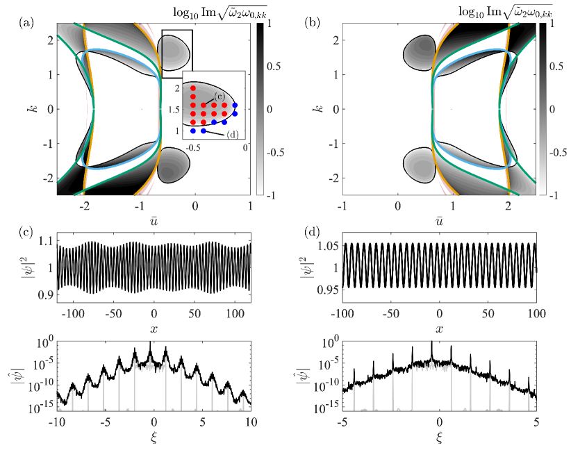
Figure 5:  Phase diagrams and numerical simulations of NLS4 two-phase solution stability. Dots in the inset of (a) correspond to solutions that are stable (blue) or unstable (red) in direct numerical simulations. See Fig. 4 and main text for details.

4.3 A model of water waves

Weakly nonlinear, nearly monochromatic wavetrains in finite-depth water waves can be modeled by the cubic NLS equation [2]

$$iA_{t}=-\frac{1}{2}\frac{d^{2}\Omega_{\rm ww,0}}{d\kappa^{2}}A_{xx}+\nu_{0}|A|^{2}A~{},$$ (55)

where $\Omega_{\rm ww}(\kappa)^{2}=\kappa\tanh\kappa$, $\Omega_{\rm ww,0}=\Omega_{\rm ww}(\kappa_{0})$, and $\nu_{0}=\nu_{0}(\kappa_{0})$ is a real constant. The NLS equation (55) is a narrow-band model, obtained by Taylor expanding the water waves linear dispersion relation $\Omega_{\rm ww}$ about the carrier wavenumber $\kappa_{0}$. More accurate models retain higher-order asymptotic terms [33]. We propose the following, analogous full-dispersion model of finite-depth water waves

$$i\psi_{t} =-\left(\widetilde{\Omega}_{\rm ww}(\kappa_{0}-i\partial_{x})-\Omega_{\rm ww,0}+ic_{{\rm g}_{0},\rm ww}\partial_{x}\right)\psi+{\rm sgn}\ \nu_{0}\ |\psi|^{2}\psi~{},$$ (56)

where $\Omega_{\rm ww,0}$ and $c_{{\rm g}_{0},\rm ww}$ are the dispersion and group velocities evaluated at $\kappa_{0}$.

A similar model was considered by Trulsen et al. [71] in deep water where the FDNLS equation (1) has dispersion $\Omega(\kappa)=\sqrt{\kappa}$. More recently, Craig, Guyenne and Sulem [26] derived a full-dispersion model of water waves that includes some of the higher-order nonlinear terms from the Dysthe equation in deep water.

To simplify the presentation, we set $\kappa_{0}=0$, which is accomplished without loss of generality by redefining the carrier wavenumber as $\overline{u}\to\overline{u}+\kappa_{0}$. To ensure that the coefficient of the nonlinear term is positive we require $\overline{u}<1.363$ so that the Benjamin-Feir instability [10] does not occur. A calculation reveals that the one-phase solutions are modulationally unstable for $\overline{u}<0$ ($\Delta_{\rm CPMI}=1$). Therefore, we omit this parameter regime and hence, we consider $0\leq\overline{u}<1.363$.

Figure 6 presents the stability regions for weakly nonlinear, fast (a) and slow (b) two-phase wavetrains. The structure of the stability phase-plane is qualitatively similar to that of the NLS3 model with third-order dispersion. In the fast branch, there are high-frequency resonant modes that co-propagate on the slow dispersion branch, so the resonance mechanism is of the same nature as in Fig. 3(a). Evaluation of $\Delta_{\rm SPMI}$ at the high-frequency resonant modes indicates that an instability is present, and one can observe this instability in numerical simulations. In large regions of parameter space, the slow two-phase waves are stable while narrow (pink) regions exhibit unstable resonant modes of the type illustrated in Fig. 3(b).

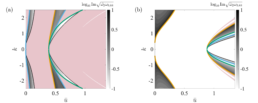
Figure 6: Phase diagrams of two-phase solution stability for the water waves model (56). See Fig. 4 and main text for details.

4.4 Discrete NLS

The defocusing, discrete NLS (DNLS) equation

$$i\psi_{n,t}=-\frac{1}{2}\left(\psi_{n-1}-2\psi_{n}+\psi_{n+1}\right)+|\psi_{n}|^{2}\psi_{n},$$ (57)

has been used, for example, to model the evolution of light in long, semiconductor waveguide arrays [60]. Significant attention has been given to the study of dark solitary wave solutions and their stability [53, 47]. To study two-phase solutions of the DNLS equation, we introduce the interpolating function $\psi(x,t)$, such that $\psi(n,t)=\psi_{n}(t)$. The shifting operators in the discrete setting can be understood in a distributional sense

$$\psi_{n\pm 1}=\psi(n\pm 1,t)=\int_{\mathbb{R}}\delta(x-n\mp 1)\psi(x,t)dx~{}.$$ (58)

The action of the advance-delay operator in the FDNLS model (1) can be represented by its Fourier transform as

$$\begin{split}\mathcal{F}\{\widetilde{\Omega}(-i\partial_{x})\psi\}&=\mathcal{F}\left\{\psi(n-1,t)-2\psi(n,t)+\psi(n+1,t)\right\}\\ &=2\left(\cos(\xi)-1\right)\widehat{\psi}(\xi,t),\end{split}$$

where $\widehat{\psi}$ is the Fourier transform of the interpolating function $\psi$. Thus, we define the continuous DNLS model as

$$i\psi_{t}=\widetilde{\Omega}(-i\partial_{x})\psi+|\psi|^{2}\psi~{}$$ (59)

with $\Omega(\xi)=1-\cos(\xi)$, whose solution is an interpolant of the solution of the DNLS equation (57). Here, the admissible range of the wavenumber is $|\overline{u}|\leq\pi/2$. The classical MI index (32) is $\Delta_{\rm CPMI}=\cos(\overline{u})$. Hence, the admissible one-phase solutions are linearly stable with respect to periodic perturbations of any wavenumber

Figure 7 presents the stability diagrams for fast and slow two-phase solutions of Eq. (59). The slow branch resembles that of a portion of the NLS4 model, Fig. 5, though a similar region containing instability islands that we explored in Sec. 4.2 is not permitted in the band-limited region of the discrete system.

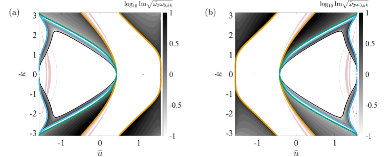
Figure 7: Phase diagrams of two-phase solution stability for the DNLS model (59). See Fig. 4 and main text for details.

5 Discussion and Conclusions

In this manuscript we derived the generalized Whitham modulation equations (23)–(26b) for the full dispersion nonlinear Schrödinger equation (1). These equations are obtained by utilizing a multiscale approach, assuming the existence of two-phase solutions, and averaging the conservation laws of the FDNLS equation over the manifold of two-phase solutions. For weak nonlinearity, the modulation equations’ type (hyperbolic / elliptic) is used to assess the MI of two-phase solutions. For the classical cubic NLS equation, the MI of one- and two-phase wavetrains is directly related. If a one-phase solution is modulationally stable (unstable) to long wavelength perturbations, then weakly nonlinear two-phase solutions with the same carrier wavenumber are also modulationally stable (unstable). One goal of this study was to identify scenarios in which the one-phase carrier wave is stable, but unstable when modulated with a finite amplitude second phase.

We obtain the characteristic velocities perturbatively and identify two distinct indices that determine the reality or complexity of these velocities. One index [Eq. (32)] corresponds to the known classical or generalized MI criterion. The new index [Eq. (49)] determines the MI of two-phase solutions. This index depends on the nonlinear potential $f$ and the linear dispersion function $\Omega(\xi)$ that define the FDNLS equation as well as the three parameters of the weakly nonlinear two-phase wavetrain: mean density $\bar{\rho}$, carrier-phase wavenumber, $\overline{u}$, and the second-phase wavenumber, $k$.

The derivation of the modulation equations and the two-phase index are obtained under general conditions. The stability predictions are determined and favorably compared with numerical simulations for the FDNLS equation with third and fourth-order dispersion. Secondary instabilities were also identified, both theoretically and numerically, resulting from linear inter- and intra-dispersion branch resonances. Nonlinearity serves to couple linearly resonant modes with different wavenumbers and the predicted instability of corresponding weakly nonlinear two-phase solutions with the same carrier wavenumber and the resonant wavenumber leads to instability. This phenomenon is studied in the FDNLS equation with third-order dispersion, which exhibits qualitatively similar features with a FDNLS model of water waves. Understanding the physical implications of these predictions, if any, is reserved for future work.

We posit that the FDNLS model provides insight into the nature of high-frequency instabilities. We note that high-frequency instabilities were observed in numerical simulations of water waves  [28] and have recently been analyzed via asymptotics and rigorous spectral methods [27, 45].

The generalized Whitham modulation equations can also be used to study solutions of initial value problems. In NLS-type equations with higher-order dispersion, distinct DSW structures emerge that have been identified with resonances [23]. These DSWs are particular, in that they may be described in terms of a shock solution of the Whitham modulation equations, an area of recent interest in nonlinear dispersive wave equations with higher-order dispersion [43, 67, 8, 7].

A novel application of the results in this manuscript are in the modulation of two-phase solutions in discrete systems, which is accomplished upon casting the advance-delay operators in these systems as a pseudodifferential operator. A promising direction of research is to utilize the Whitham modulation theory developed here to study DSW structures that evolve from step-like initial data in full-dispersion NLS models, such as the discrete NLS equation.

References

- [1] M. J. Ablowitz, Nonlinear Dispersive Waves: Asymptotic Analysis and Solitons, Cambridge University Press, 2011.
- [2] M. J. Ablowitz and H. Segur, Solitons and Inverse Scattering Transform, SIAM, Philadelphia, 1981.
- [3] P. Aceves-Sanchez, A. Minzoni, and P. Panayotaros, Numerical study of a nonlocal model for water-waves with variable depth, Wave Motion, 50 (2013), pp. 80–93.
- [4] G. P. Agrawal, Nonlinear Fiber Optics, in Nonlinear Science at the Dawn of the 21st Century, Springer, 2000, pp. 195–211.
- [5] S. Amiranashvili and E. Tobisch, Extended criterion for the modulation instability, New J. Phys., 21 (2019), p. 033029.
- [6] A. Ankiewicz, Y. Wang, S. Wabnitz, and N. Akhmediev, Extended nonlinear Schrödinger equation with higher-order odd and even terms and its rogue wave solutions, Phys. Rev. E, 89 (2014), p. 012907.
- [7] S. Baqer, D. J. Frantzeskakis, T. P. Horikis, C. Houdeville, T. R. Marchant, and N. F. Smyth, Nematic dispersive shock waves from nonlocal to local, Applied Sciences, 11 (2021), p. 4736.
- [8] S. Baqer and N. F. Smyth, Modulation theory and resonant regimes for dispersive shock waves in nematic liquid crystals, Physica D, 403 (2020), p. 132334.
- [9] T. B. Benjamin, Instability of periodic wavetrains in nonlinear dispersive systems, P. Roy. Soc. A, 299 (1967), pp. 59–76.
- [10] T. B. Benjamin and J. E. Feir, The disintegration of wave trains on deep water Part 1. Theory, Journal of Fluid Mechanics, 27 (1967), pp. 417–430.
- [11] S. Benzoni-Gavage, C. Mietka, and L. M. Rodrigues, Modulated equations of Hamiltonian PDEs and dispersive shocks, Nonlinearity, 34 (2021), p. 578.
- [12] S. Benzoni-Gavage, P. Noble, and L. M. Rodrigues, Slow Modulations of Periodic Waves in Hamiltonian PDEs, with Application to Capillary Fluids, J. Nonlinear Sci., 24 (2014), pp. 711–768.
- [13] V. I. Bespalov and V. I. Talanov, Filamentary structure of light beams in nonlinear liquids, JETP Lett., 3 (1966), p. 307.
- [14] A. L. Binswanger, M. A. Hoefer, B. Ilan, and P. Sprenger, Whitham modulation theory for generalized Whitham equations and a general criterion for modulational instability, Stud. Appl. Math., 147 (2021), pp. 724–751.
- [15] G. Biondini, Riemann problems and dispersive shocks in self-focusing media, Phys. Rev. E, 98 (2018).
- [16] G. Biondini, G. El, M. Hoefer, and P. Miller, Dispersive hydrodynamics: Preface, Physica D, 333 (2016), pp. 1–5.
- [17] G. Biondini and D. Mantzavinos, Universal nature of the nonlinear stage of modulational instability, Phys. Rev. Lett., 116 (2016), p. 043902.
- [18] , Long-time asymptotics for the focusing nonlinear Schrödinger equation with nonzero boundary conditions at infinity and asymptotic stage of modulational instability, Comm. Pure Appl. Math., 70 (2017), pp. 2300–2365.
- [19] N. Bottman, B. Deconinck, and M. Nivala, Elliptic solutions of the defocusing NLS equation are stable, J. Phys. A-Math. Gen., 44 (2011), p. 285201.
- [20] J. C. Bronski and M. A. Johnson, The modulational instability for a generalized Korteweg–de Vries equation, Archive for Rational Mechanics and Analysis, 197 (2010), pp. 357–400.
- [21] J. D. Carter, Bidirectional Whitham equations as models of waves on shallow water, Wave Motion, 82 (2018), pp. 51–61.
- [22] W. A. Clarke, R. Marangell, and W. R. Perkins, Rigorous justification of the Whitham modulation equations for equations of Whitham type, Stud. Appl. Math., 149 (2022), pp. 297–323.
- [23] M. Conforti, F. Baronio, and S. Trillo, Resonant radiation shed by dispersive shock waves, Phys. Rev. A, 89 (2014), p. 013807.
- [24] M. Conforti and S. Trillo, Dispersive wave emission from wave breaking, Opt. Lett., 38 (2013), pp. 3815–3818.
- [25] , Radiative effects driven by shock waves in cavity-less four-wave mixing combs, Opt. Lett., 39 (2014), pp. 5760–5763.
- [26] W. Craig, P. Guyenne, and C. Sulem, Normal Form Transformations and Dysthe’s Equation for the Nonlinear Modulation of Deep-Water Gravity Waves, Water Waves, (2020).
- [27] R. P. Creedon, B. Deconinck, and O. Trichtchenko, High-frequency instabilities of Stokes waves, J. Fluid Mech., 937 (2022), p. A24.
- [28] B. Deconinck and K. Oliveras, The instability of periodic surface gravity waves, J. Fluid Mech., 675 (2011), pp. 141–167.
- [29] B. Deconinck and B. L. Segal, The stability spectrum for elliptic solutions to the focusing NLS equation, Physica D, 346 (2017), pp. 1–19.
- [30] E. Dinvay, H. Kalisch, D. Moldabayev, and E. I. Părău, The Whitham equation for hydroelastic waves, Applied Ocean Research, 89 (2019), pp. 202–210.
- [31] K. Dysthe, H. E. Krogstad, and P. Müller, Oceanic rogue waves, Annu. Rev. Fluid Mech., 40 (2008), pp. 287–310.
- [32] K. B. Dysthe, Note on a modification to the nonlinear Schrödinger equation for application to deep water waves, P. Roy. Soc. A, 369 (1979), pp. 105–114.
- [33] K. B. Dysthe, Note on a Modification to the Nonlinear Schrodinger Equation for Application to Deep Water Waves, P. R. Soc. As, 369 (1979), pp. 105–114.
- [34] G. A. El, V. V. Geogjaev, A. V. Gurevich, and A. L. Krylov, Decay of an initial discontinuity in the defocusing NLS hydrodynamics, Physica D, 87 (1995), pp. 186–192.
- [35] G. A. El, R. H. J. Grimshaw, and N. F. Smyth, Unsteady undular bores in fully nonlinear shallow-water theory, Phys. Fluids, 18 (2006), pp. 027104–17.
- [36] G. A. El, A. V. Gurevich, V. V. Khodorovskii, and A. L. Krylov, Modulational instability and formation of a nonlinear oscillatory structure in a ”focusing” medium, Phys. Lett. A, 2 (1993), p. 1.
- [37] G. A. El and M. A. Hoefer, Dispersive shock waves and modulation theory, Physica D, 333 (2016), pp. 11–65.
- [38] G. A. El, E. G. Khamis, and A. Tovbis, Dam break problem for the focusing nonlinear Schrödinger equation and the generation of rogue waves, Nonlinearity, 29 (2016), pp. 2798–2836.
- [39] G. A. El and A. L. Krylov, General solution of the Cauchy problem for the defocusing NLS equation in the Whitham limit, Phys. Lett. A, 203 (1995), pp. 77–82.
- [40] M. G. Forest and J.-E. Lee, Geometry and modulation theory for the periodic nonlinear Schrödinger equation, in Oscillation Theory, Computation, and Methods of Compensated Compactness, vol. 2, Springer, 1986, pp. 35–69.
- [41] A. Gelash, D. Agafontsev, V. Zakharov, G. El, S. Randoux, and P. Suret, Bound State Soliton Gas Dynamics Underlying the Spontaneous Modulational Instability, Phys. Rev. Lett., 123 (2019).
- [42] S. Gustafson, S. Le Coz, and T.-P. Tsai, Stability of periodic waves of 1d cubic nonlinear schrödinger equations, Appl. Math. Res. Express, 2017 (2017), pp. 431–487.
- [43] M. A. Hoefer, N. F. Smyth, and P. Sprenger, Modulation theory solution for nonlinearly resonant, fifth-order Korteweg-de Vries, nonclassical, traveling dispersive shock waves, Stud. Appl. Math., 142 (2019), pp. 219–240.
- [44] V. M. Hur and A. K. Pandey, Modulational instability in a full-dispersion shallow water model, Stud. Appl. Math., 142 (2019), pp. 3–47.
- [45] V. M. Hur and Z. Yang, Unstable Stokes Waves, Arch. Ration. Mech. Anal., 247 (2023), p. 62.
- [46] S. Jin, C. D. Levermore, and D. W. McLaughlin, The semiclassical limit of the defocusing NLS hierarchy, Commun. Pur. Appl. Math., 52 (1999), pp. 613–654.
- [47] M. Johansson and Y. S. Kivshar, Discreteness-Induced Oscillatory Instabilities of Dark Solitons, Phys. Rev. Lett., 82 (1999), pp. 85–88.
- [48] M. A. Johnson and W. R. Perkins, Modulational Instability of Viscous Fluid Conduit Periodic Waves, SIAM J. Math. Anal., (2020), pp. 277–305.
- [49] Johnson M. A. and Zumbrun K., Rigorous Justification of the Whitham Modulation Equations for the Generalized Korteweg-de Vries Equation, Stud. Appl. Math., 125 (2010), pp. 69–89.
- [50] R. I. Joseph, Solitary waves in a finite depth fluid, J. Phys. A-Math. Gen., 10 (1977), pp. L225–L227.
- [51] A. M. Kamchatnov, Nonlinear periodic waves and their modulations: an introductory course, World Scientific, 2000.
- [52] C. Kharif and M. Abid, Nonlinear water waves in shallow water in the presence of constant vorticity: A Whitham approach, Eur. J. Mech. B-Fluid., 72 (2018), pp. 12–22.
- [53] Kivshar, Y. S. and Królikowski, W. and Chubykalo, Oksana A., Dark solitons in discrete lattices, Phys. Rev. E, 50 (1994), pp. 5020–5032.
- [54] Y. Kodama, The Whitham equations for optical communications: Mathematical theory of NRZ, SIAM J. Appl. Math, 59 (1999), pp. 2162–2192.
- [55] D. Lannes, The Water Waves Problem: Mathematical Analysis and Asymptotics, American Mathematical Society, 2013.
- [56] P. D. Lax, The Formation and Decay of Shock Waves, The American Mathematical Monthly, 79 (1972), pp. 227–241.
- [57] S. Malaguti, M. Conforti, and S. Trillo, Dispersive radiation induced by shock waves in passive resonators, Opt. Lett., 39 (2014), p. 5626.
- [58] T. Marest, F. Braud, M. Conforti, S. Wabnitz, A. Mussot, and A. Kudlinski, Longitudinal soliton tunneling in optical fiber, Opt. Lett., 42 (2017), pp. 2350–2353.
- [59] D. Moldabayev, H. Kalisch, and D. Dutykh, The Whitham Equation as a model for surface water waves, Physica D, 309 (2015), pp. 99–107.
- [60] R. Morandotti, U. Peschel, J. Aitchison, H. Eisenberg, and Y. Silberberg, Dynamics of discrete solitons in optical waveguide arrays, Physical Review Letters, 83 (1999), p. 2726.
- [61] A. Newell, Solitons in Mathematics and Physics, CBMS-NSF Regional Conference Series in Applied Mathematics, Society for Industrial and Applied Mathematics, Jan. 1985.
- [62] L. Ostrovskii, Propagation of wave packets and space-time self-focusing in a nonlinear medium, Sov. Phys. JETP, 24 (1967), pp. 797–800.
- [63] M. V. Pavlov, Nonlinear Schrödinger equation and the Bogolyubov-Whitham method of averaging, Teor. Mat. Fiz., 71 (1987), pp. 584–588.
- [64] M. Potasek, Modulation instability in an extended nonlinear Schrödinger equation, Opt. Lett., 12 (1987), pp. 921–923.
- [65] Y. V. Sedletsky, The fourth-order nonlinear Schrödinger equation for the envelope of Stokes waves on the surface of a finite-depth fluid, J. Exp. Theor. Phys., 97 (2003), pp. 180–193.
- [66] A. Slunyaev, A high-order nonlinear envelope equation for gravity waves in finite-depth water, J. Exp. Theor. Phys., 101 (2005), pp. 926–941.
- [67] P. Sprenger and M. A. Hoefer, Discontinuous shock solutions of the Whitham modulation equations as zero dispersion limits of traveling waves, Nonlinearity, 33 (2020), pp. 3268–3302.
- [68] G. G. Stokes, On the theory of oscillatory waves, Trans. Camb. Phil. Soc., 8 (1847), pp. 441–455.
- [69] V. Talanov, Self focusing of wave beams in nonlinear media, ZhETF Pisma Redaktsiiu, 2 (1965), p. 218.
- [70] S. Trillo, M. Klein, G. Clauss, and M. Onorato, Observation of dispersive shock waves developing from initial depressions in shallow water, Physica D, 333 (2016), pp. 276–284.
- [71] K. Trulsen and K. B. Dysthe, A modified nonlinear Schrodinger equation for broader bandwidth gravity waves on deep water, Wave Motion, 24 (1996), pp. 281–289.
- [72] K. Trulsen, I. Kliakhandler, K. B. Dysthe, and M. G. Velarde, On weakly nonlinear modulation of waves on deep water, Phys. Fluids, 12 (2000), pp. 2432–2437.
- [73] M. P. Tulin and T. Waseda, Laboratory observations of wave group evolution, including breaking effects, J. Fluid Mech., 378 (1999), pp. 197–232.
- [74] G. B. Whitham, Non-linear dispersive waves, Proc. Roy. Soc. Ser. A, 283 (1965), pp. 238–261.
- [75] , Variational methods and applications to water waves, P. R. Soc. A, 299 (1967), pp. 6–25.
- [76] , Linear and nonlinear waves, Wiley, New York, 1974.
- [77] J. Yang, Newton-conjugate-gradient methods for solitary wave computations, Journal of Computational Physics, 228 (2009), pp. 7007–7024.
- [78] , Nonlinear waves in integrable and nonintegrable systems, SIAM, 2010.
- [79] H. Yoshida, Construction of higher order symplectic integrators, Physics letters A, 150 (1990), pp. 262–268.
- [80] V. Zakharov and L. Ostrovsky, Modulation instability: The beginning, Physica D, 238 (2009), pp. 540–548.
- [81] V. E. Zakharov, Stability of periodic waves of finite amplitude on the surface of a deep fluid, Journal of Applied Mechanics and Technical Physics, 9 (1972), pp. 190–194.
- [82] J. Zhang, S. Wen, Y. Xiang, and H. Luo, General features of spatiotemporal instability induced by arbitrary high-order nonlinear dispersions in metamaterials, J. Mod. Optic., 57 (2010), pp. 876–884.