Towards Green AI in Fine-tuning Large Language Models via Adaptive Backpropagation

Abstract

Fine-tuning is the most effective way of adapting pre-trained large language models (LLMs) to downstream applications. With the fast growth of LLM-enabled AI applications and democratization of open-souced LLMs, fine-tuning has become possible for non-expert individuals, but intensively performed LLM fine-tuning worldwide could result in significantly high energy consumption and carbon footprint, which may bring large environmental impact. Mitigating such environmental impact towards Green AI directly correlates to reducing the FLOPs of fine-tuning, but existing techniques on efficient LLM fine-tuning can only achieve limited reduction of such FLOPs, due to their ignorance of the backpropagation cost in fine-tuning. To address this limitation, in this paper we present GreenTrainer, a new LLM fine-tuning technique that adaptively evaluates different tensors’ backpropagation costs and contributions to the fine-tuned model accuracy, to minimize the fine-tuning cost by selecting the most appropriate set of tensors in training. Such selection in GreenTrainer is made based on a given objective of FLOPs reduction, which can flexibly adapt to the carbon footprint in energy supply and the need in Green AI. Experiment results over multiple open-sourced LLM models and abstractive summarization datasets show that, compared to fine-tuning the whole LLM model, GreenTrainer can save up to 64% FLOPs in fine-tuning without any noticeable model accuracy loss. Compared to the existing fine-tuning techniques such as LoRa, GreenTrainer can achieve up to 4% improvement on model accuracy with on-par FLOPs reduction. GreenTrainer has been open-sourced at: https://github.com/pittisl/GreenTrainer.

1 Introduction

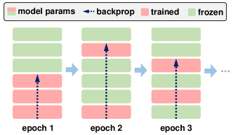
Figure 1: GreenTrainer adaptively selects the trainable portion

Large language models (LLMs), being pre-trained on large-scale text data, have been used as foundational tools in generative AI for natural language generations. The most effective way of adapting LLMs to downstream applications, such as personal chat bots and podcast summarizers, is to fine-tune a generic LLM using the specific application data [11]. Intuitively, fine-tuning is less computationally expensive than pre-training due to the smaller amount of training data, but it may result in significantly high energy consumption and carbon footprint when being intensively performed worldwide and hence bring large environmental impact. In particular, enabled by the democratization of open-sourced LLMs [8] and convenient APIs of operating these LLMs [32; 41], even non-expert individuals can easily fine-tune LLMs using a few lines of codes, either for performance enhancement or model personalization [37]. For example, when a LLaMA-13B model [39] is fine-tuned by 10k users using A100-80GB GPUs, such fine-tuning consumes 6.9$\times$ more GPU hours than pre-training a GPT-3 model [6] with 175B parameters. The amount of energy being consumed by such fine-tuning, correspondingly, is comparable to those consumed by small towns or even some underdeveloped countries, and the amount of emitted carbon dioxide is equivalent to 500$\times$ of that produced by a New York-San Francisco round-trip flight [1].

Mitigating such environmental impact towards Green AI directly correlates to reducing the number of floating operations (FLOPs) of fine-tuning, as FLOPs is a fundamental measure that represents the amount of computational operations and hence energy consumption in training [36]. Most existing techniques, however, are limited to optimizing LLM fine-tuning for lower memory consumption rather than FLOPs reduction [29; 24]. Some other methods reduce the amount of computations by only fine-tuning specific types of model parameters such as bias [42], LayerNorm and output layer weights [28], but they significantly impair the model’s expressivity and are only applicable to simple non-generative learning tasks. Instead, researchers suggested keeping the original model parameters frozen but injecting additional trainable parameters either to the input [21; 26] or internal layers [23; 17]. Recent LoRA-based methods [16; 43] further reduce the overhead of computing weight updates for these injected parameters via low-rank approximation. These methods can achieve comparable accuracy on generative tasks with full fine-tuning. However, they still need to compute the activation gradients through the whole model, and their FLOPs reduction is hence limited to computations of weight updates, which are only 25%-33% of the total training FLOPs.

Besides computing weight updates, FLOPs in training are also produced in i) forward propagation and ii) backward propagation of activation gradients. Since complete forward propagation is essential to calculate the training loss, we envision that the key to effective FLOPs reduction is to take the backpropagation cost of activation gradients, which is at least another 33% of the total training FLOPs, into account and selectively involve only the most appropriate model structures in backpropagation. The major challenge, however, is that such selective training will nearly always bring model accuracy loss. Our basic idea to minimize the accuracy loss is to adapt such selection in backpropagation to a flexible objective of FLOPs reduction, which is determined by the carbon footprint in energy supply for LLM fine-tuning. For example, when such carbon footprint is low due to more insertion of renewable energy, a lower objective of FLOPs reduction can be used to retain more model structures to training and hence retain the training accuracy. On the other hand, high carbon footprint in energy production could lead to a higher objective of FLOPs reduction for better embracing Green AI.

Based on this idea of adaptive backpropagation, in this paper we present GreenTrainer, a new training technique for efficient LLM fine-tuning with the minimum accuracy loss. As shown in Figure 1, given an objective of FLOPs reduction, GreenTrainer adaptively selects the most appropriate set of trainable neural network (NN) tensors at run-time, based on evaluation of different tensors’ importance in training. Such importance evaluation is difficult because NN tensors do not directly associate with any input data variables or intermediate features, and most attribution techniques [38; 15] that evaluate feature importance are hence not applicable. Traditional approaches based on weight magnitudes [22], random perturbations [5], and gating functions [14], on the other hand, are either inaccurate or computationally expensive for LLMs. Instead, our approach is to follow a similar rationale with current attribution techniques that measures the importance of an input data variable as the accumulation of relevant gradients, to evaluate tensor importance as the cumulative gradient changes of its weight updates in training. In this way, we ensure that selected tensors will make the maximum contribution to reducing the training loss.

Another challenge is how to precisely profile the training FLOPs of different tensor selections. Due to the interdependency between different tensors, their total FLOPs in training is usually not equal to the summation of their individual training FLOPs. Such interdependency is determined by the backpropagation characteristics of the specific NN operators connected to each tensor, but existing FLOPs models cannot link NN operators to tensors based on the computing flow of backpropagation. To tackle this challenge, we build a new FLOPs model that incorporates the relations between tensors and NN operations into profiling of training FLOPs. Based on this model, we develop a dynamic programming (DP) algorithm that can find the nearly optimal tensor selection from an exponential number of possibilities (e.g., $2^{515}$ for 515 tensors in OPT-2.7B model [44]), with negligible computing overhead.

We evaluated the training performance of GreenTrainer with three open-sourced LLMs, namely OPT [44], BLOOMZ [30] and FLAN-T5 [10], on text generation datasets including SciTLDR [7] and DialogSum [9]. Our experiment results show that GreenTrainer can save up to 64% training FLOPs compared to full LLM fine-tuning, without any noticeable accuracy loss. In some cases, GreenTrainer can even improve the model accuracy compared to that of full fine-tuning, by removing model redundancy and hence mitigating the model overfitting. Compared to existing fine-tuning techniques such as Prefix Tuning [23] and LoRA [16], GreenTrainer can improve the model accuracy by 4%, with the same amount of FLOPs reduction, and also provides users with the flexibility to balance between the training accuracy and cost depending on the specific needs of green AI.

2 Background & Motivation

2.1 Transformer Architectures for Text Generation

Current LLMs are stacked by transformer blocks [40], each of which contains a Multi-Head Attention (MHA) layer, LayerNorms [4], and a Feed-Forward Network (FFN) with two dense layers. Given an input sequence $X\in\mathbb{R}^{n\times d}$ with $n$ tokens, the MHA separately projects all the tokens into a $(Q,K,V)$ space $h$ times, using $h$ suites of trainable projectors $(W_{Q}^{(i)},W_{K}^{(i)},W_{V}^{(i)})_{i=1,...,h}$. Each projection $f_{i}:\mathbb{R}^{n\times d}\to\mathbb{R}^{n\times\frac{d}{h}}$ is defined as:

$$Q_{i},K_{i},V_{i}=XW_{Q}^{(i)},XW_{K}^{(i)},XW_{V}^{(i)}.\vspace{-0.05in}$$ (1)

The output $(Q_{i},K_{i},V_{i})$ then performs attention mechanisms to produce $O_{i}$ by weighting $V_{i}$ with the attention scores between $Q_{i}$ and $K_{i}$. The MHA’s final output is obtained by concatenating each $O_{i}$, following a linear projection $g:\mathbb{R}^{n\times d}\to\mathbb{R}^{n\times d}$ with a trainable projector $W_{o}$:

$$O_{i} =\mathrm{Softmax}\left(Q_{i}K_{i}^{\top}/\sqrt{d/h}\right)V_{i}, \mathrm{MHA_{out}}=\mathrm{Concat}(O_{1},O_{2},...,O_{h})W_{o}.$$ (2)

Due to their auto-regressive nature, LLMs can only generate a single output token in each forward pass, which is inefficient in training. Instead, LLMs adopt the teacher-forcing method [19] to generate the entire sequence of output tokens in a single forward pass. Specifically, causal masks are applied to MHA’s attention scores, so that each output token can be predicted from the label tokens at previous positions. With this technique, when being fine-tuned, LLMs can be trained in a standard way like any feed-forward models.

2.2 The Need for Adaptive Backpropagation

By stacking a sufficient number of large transformer blocks, pre-trained LLMs can capture general language patterns and world knowledge. However, when being fine-tuned for a downstream task, they are usually over-parameterized because only part of the world knowledge they learned is useful for the target task. In these cases, only involving some of the model’s substructures into fine-tuning could have little impact on the model accuracy, but significantly reduces the amount of computations.

Trainable substructure	OPT-2.7B		FLAN-T5-3B
	FLOPs ($\times 10^{15}$)	Acc. (%)	FLOPs ($\times 10^{15}$)	Acc. (%)
All params	262.0	23.6	135.7	46.5
Last 2 layers	181.6 (31%$\downarrow$)	20.8	46.1 (66%$\downarrow$)	39.2
Decoder prefix	174.7 (33%$\downarrow$)	13.4	55.3 (60%$\downarrow$)	37.6
$(W_{Q},W_{V})$	174.7 (33%$\downarrow$)	23.8	90.5 (33%$\downarrow$)	44.7

Table 1: Fine-tuning different substructures of OPT-2.7B and FLAN-T5-3B LLMs on the DialogSum dataset (ROUGE-1 score on the test set is used as the accuracy metric)

Existing work has made attempts with fixed selections of some NN components, such as the last 2 layers, decoder prefixes [23], and linear projectors $(W_{Q},W_{V})$ [16], to be involved in fine-tuning. However, due to the interdependencies of NN parameters [18], using such fixed selections for fine-tuning will significantly impair the trained model’s accuracy. As shown in Table 1, solely fine-tuning either the last 2 layers or decoder prefixes leads to up to 10 % accuracy drop compared to full fine-tuning. The major reason is that the nearby NN substructures that have interdependencies with the fixed selections have been excluded from fine-tuning, and hence become inconsistent with those selected substructures. Increasing the density of selected substructures, such as including all the linear projectors $(W_{Q},W_{V})$, could mitigate the model accuracy loss caused by such inconsistency, but can only save at most 33% FLOPs due to backpropagating activation gradients through all the transformer blocks. Some naive methods of dynamic selections, such as progressively expanding the trainable portion from the last layer, have the similar limitation in FLOPs reduction.

The deficiency of these existing methods motivates us to enforce more flexible and adaptive selection of LLM substructures in backpropagation. In GreenTrainer, we develop a tensor importance metric that incorporates parameter dependencies to evaluate how fine-tuning each tensor contributes to the trained model’s accuracy at runtime. Knowledge about such tensor importance, then, allows us to achieve the desired FLOPS reduction while maximizing the model accuracy.

2.3 FLOPs Model of Backpropagation

The design of GreenTrainer relies on proper calculation of the selected model substructures’ backpropagation FLOPs, which can be decomposed into two parts using the chain rule. For example, as shown in Figure 2, when training a 4-layer dense NN without bias, each layer computes i) $\mathrm{dy_{i}}$ as the loss $L$’s gradient w.r.t the activation $y_{i}$, and ii) $\mathrm{dw_{i}}$ as the loss gradient w.r.t weight $W_{i}$, such that

$$\mathrm{dy_{i}} =\frac{\partial L}{\partial y_{i}}=\frac{\partial L}{\partial y_{i+1}}W_{i}^{\top}=\mathrm{dy_{i+1}}W_{i}^{\top}, \mathrm{dw_{i}}=\frac{\partial L}{\partial W_{i}}=y_{i}^{\top}\frac{\partial L}{\partial y_{i+1}}=y_{i}^{\top}\mathrm{dy_{i+1}},$$ (3)

and the corresponding amount of FLOPs for computing $\mathrm{dy_{i}}$ and $\mathrm{dw_{i}}$ can be denoted as $t_{dy_{i}}$ and $t_{dw_{i}}$, respectively.

$(\mathrm{dy_{i}},\mathrm{dw_{i}})$ can be computed from the upstream $(\mathrm{dy_{i+1}},\mathrm{dw_{i+1}})$. In particular, even if a layer is not selected in fine-tuning, it still needs to compute and pass error gradients ($\mathrm{dy_{i}}$) to the downstream layers. Hence, the amount of computations in backpropagation do not only depend on the selected layers, but also depends on some unselected layers. For example, if only Layer 2 is trainable and all other layers are frozen, the total FLOPs for backpropagation includes i) the FLOPs of computing $\mathrm{dw_{2}}$ and i) the FLOPs of computing $\mathrm{dy_{3}}$ and $\mathrm{dy_{4}}$. Due to the generality of the chain rule, such rationale of FLOPs calculation is also applicable to other types of NN layers.

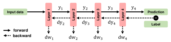
Figure 2: Backpropagation of a 4-layer dense NN

Based on this rationale, we can construct FLOPs models for LLM substructures, including MHA and FFN. However, the layer-level time model is coarse-grained and can lead to inaccurate selection of the trainable portion in LLM fine-tuning. Some important parameters may be unselected because many others within the same layer are unimportant. In GreenTrainer, we push the selection granularity to the tensor level, which can be well-supported by tensorized NN libraries (e.g., TensorFlow [2] and PyTorch [33]). On the other hand, although the weight-level selection is more fine-grained, it also requires fine-grained indexing and incurs unnecessarily high overhead.

3 GreenTrainer Method

To reduce the FLOPs of LLM fine-tuning, an intuitive problem formulation is to minimize the FLOPs while achieving the desired objective of the fine-tuned model accuracy. However, it is generally hard to determine an appropriate accuracy objective in advance, because some accuracy objectives may require very intensive training and the accuracy that we can achieve with our FLOPs budget cannot be pre-estimated before training. Instead, GreenTrainer aims to maximize the training loss reduction while achieving the desired FLOPs reduction, as formulated below:

$$\max{\Delta_{loss}(\bm{m})}\ \ \ \text{s.t.}\ \ T_{selective}(\bm{m})\leq\rho T_{full},$$ (4)

where $\bm{m}$ is a binary selector to be solved for selecting the appropriate set of tensors in fine-tuning. $\bm{m}$ parametrizes both the loss reduction ($\Delta_{loss}$) and the per-batch FLOPs of training ($T_{selective}$), and $T_{selective}$ is constrained to be lower than a user-specified ratio ($\rho$) of the per-batch training FLOPs of fine-tuning the whole model ($T_{full}$). For example, $\rho=0.5$ means that the FLOPs of fine-tuning should be reduced to 50% of that in fine-tuning the whole model. In practice, depending on the specific LLM fine-tuning scenario, the value of $\rho$ can either be preset prior to training, or dynamically adjusted at runtime in any stage of training.

To clearly identify each tensor’s contribution in fine-tuning, we model $\Delta_{loss}(\bm{m})$ as the aggregated importance of the selected tensors in training, and calculate the FLOPs incurred by the selected tensors using the FLOPs model of backpropagation being described in Section 2.3. With this FLOPs model, Eq. 4 can be rewritten as:

$$\max{\ \Delta_{loss}(\bm{m})}\ \ \ \ \ \text{s.t.}\ \ T_{fp}+\bm{m}\cdot\bm{t}_{dw}+\sigma(\bm{m})\cdot\bm{t}_{dy}\leq\rho T_{full},$$ (5)

where $T_{fp}$ indicates the per-batch FLOPs of the forward pass, and each pair of variables in $(\bm{t}_{dy},\bm{t}_{dw})$ represents the FLOPs of computing $(\mathrm{dy},\mathrm{dw})$ for the corresponding tensor, respectively. Given a binary selector $\bm{m}$, $\sigma(\bm{m})$ incorporates all the tensors along the backward pass that contribute to the FLOPs of fine-tuning, by involving in passing the error gradients ($\mathrm{dy}$). For example, if $\bm{m}=[0,0,1,0,1,0,0]$, all the tensors that are in deeper layers than the selected tensors are involved in passing the error gradients, and hence $\sigma(\bm{m})=[0,0,1,1,1,1,1]$.

To ground the above formulation and solve $\bm{m}$, GreenTrainer consists of three key components: (i) Tensor FLOPs Profiling, which calculates the FLOPs of all NN tensors (i.e., $\bm{t}_{dy}$ and $\bm{t}_{dw}$) prior to training; (ii) Tensor Importance Evaluation, which quantifies the contribution of updating each NN tensor to the training quality at runtime; (iii) Tensor Selector, which grounds the tensor selection problem using tensors’ FLOPs and importances, and provides solutions via dynamic programming at runtime.

3.1 Tensor FLOPs Profiling

Standard NN profilers, such as the Torch Profiler [33], can measure the execution FLOPs of individual NN operators, such as matrix multiplication and convolution. However, such profiling of NN operators cannot be directly linked to the corresponding NN tensors that participate in these operations. In other words, when a set of selected tensors is trained, the training FLOPs of backpropagation are not equal to the summation of individual tensors’ backpropagtion FLOPs.

To address this limitation, our approach consists of two steps. First, we convert the layer-based NN structure of LLMs into a tensor-level computing graph, which retains the execution order of all tensors’ involvements in training. Then, we extract the related backpropagation operators of each tensor, and derive each tensor $i$’s FLOPs in backpropagation ($t_{dy_{i}}$ and $t_{dw_{i}}$) by matching and aggregating the FLOPs of these NN operators. For example in Figure 3, the training of each linear projector ($Q$, $K$ and $V$) in an MHA layer should be executed after its corresponding bias tensor’s training. Training each linear projector, then, will involve two matrix multiplication operators, whose FLOPs in backpropagation will be aggregated. We categorize such rules of matching and aggregation by the type of LLM layers where tensors are located, as described below.

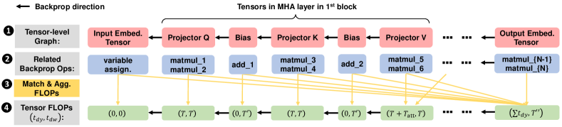
Figure 3: An sample workflow of tensor FLOPs profiling

Input & output embedding layers. The input embedding layer contains a trainable embedding tensor that maps each raw token into a dense representation through efficient lookup operations. Given the activation gradient $\rm{dy_{i+1}}$ from upstream layers, deriving the update $\rm{dw_{i}}$ of this embedding tensor only involves variable assignment without any heavy computations. Hence, we can safely consider $t_{dw_{i}}\approx 0$ for any tensor $i$. Specifically, if a raw token is mapped to the $k$-th vector in the embedding tensor during the forward pass, then during backpropagation, $\rm{dy_{i+1}}$ from the upstream will be only assigned to $k$-th row of $\rm{dw_{i}}$, such that

$${\rm{dw_{i}}}[s]={\rm{dy_{i+1}}}\ \text{if}\ s=k,\ \text{else}\ \bm{0}.$$ (6)

Since the input layer doesn’t propagate activation gradients, we can also conclude that its $t_{dy}$ is 0.

Reversely, the output embedding layer projects each token back to the probability space by multiplying its trainable tensor with the token vector. Intuitively, its $(t_{dy},t_{dw})$ can be derived in the same way as we did for the dense NN layer in Eq. (3). However, in most LLMs, the output embedding layer shares the same trainable tensor with the input embedding layer. This implies that if the output embedding is trainable, then the input embedding will also be involved in training. To reflect this correlation, all the $t_{dy}$ from the LLM’s output, up to the input embedding layer, should be accumulated to the $t_{dy}$ of the output embedding tensor, while its $t_{dw}$ remains unchanged.

Multi-Head Attention (MHA) layer. As described in Section 2.2, a MHA layer contains multiple linear projectors as trainable tensors, and their FLOPs in training can be generally derived in the same way as we did with the dense NN layer. In addition, some LLMs such as OPT also include bias as another type of trainable tensor after such projection. In this case, based on the chain rule, the backpropagation of bias is computed as:SS

$${\rm{dy_{i}}} ={\rm{dy_{i+1}}}, {\rm{dw_{i}}} =\bm{1}^{\top}{\rm{dy_{i+1}}},$$ (7)

which indicates that $t_{dy}$ for bias is 0 since ${\rm{dy_{i}}}$ is identically passed from ${\rm{dy_{i+1}}}$. $t_{dw}$ of bias can be derived as the FLOPs of adding up the elements in ${\rm{dy_{i+1}}}$, along every embedding feature channel.

The attention mechanism in Eq. (2) is backpropagated prior to the projectors. If any of these projectors are involved in training, the attention’s backpropagation FLOPs must be also calculated. To do this, we accumulate such FLOPs to the corresponding projector tensor ($W_{V}$)’s $t_{dy}$.

LayerNorm. Given a token, LayerNorm first normalizes its features and then uses two trainable tensors $\gamma$ and $\beta$ to element-wise multiply with and add to the token, respectively. The operations of multiplication and addition are similar to those in the dense NN layer, and so its FLOPs can also be calculated in the similar way. However, the backpropagation FLOPs of normalization operators should be accumulated to the previous tensor’s $t_{dy}$. That means if any tensors in the previous layers are trained, the FLOPs of propagating the normalization operators should be also included when calculating the FLOPs of the current layer.

Feed-Forward Network (FFN). In the FFN, there is a nonlinear activation function between two dense layers. Following the same method of calculating LayerNorm’s FLOPs, we accumulate the FLOPs of propagating through this activation function to the bias tensor’s $t_{dy}$ in the first dense layer.

3.2 Tensor Importance Evaluation

Generally speaking, a tensor’s importance in training can be estimated as the summation of the importances of all its weights. In training, since the model weights are iteratively updated to minimize the training loss, an intuitive approach to evaluating the importance of a weight update in a given iteration is to undo this update and check how the training loss increases back:

$$\Delta L=L(w)-L(w+\Delta w),$$ (8)

so that a higher value of $\Delta L$ means this update is more important and the corresponding weight should be selected for fine-tuning. However, repeatedly applying this approach to every NN weight is expensive due to the large number of weights in LLMs. Instead, our approach is to estimate the importance of all the NN weights in one shot by utilizing the information available in the backpropagation procedure. More specifically, we compute the importance of each weight by smoothing the undo operation described above and computing the loss gradients with respect to the updates that correspond to all the weights. Letting the multiplicative $\bm{c}\in[0,1]^{M}$ denote the continuous undo operation for all the $M$ weights in the model, we can compute the loss gradient with respect to $\bm{c}$ as

$$-\frac{\partial L(\bm{w}+\bm{c}\odot\Delta\bm{w})}{\partial\bm{c}}=-\left.\Delta\bm{w}\odot\frac{\partial L(\bm{u})}{\partial\bm{u}}\right|_{\bm{u}=\bm{w}+\bm{c}\odot\Delta\bm{w}},$$ (9)

where $\odot$ denotes element-wise multiplication. When $\bm{c}=\bm{0}$, Eq. (9) becomes an importance vector where each element corresponds to a model weight. Since the loss gradient is parametrized by all the model weights, the weight importances calculated in this way implicitly incorporate the impact of weight dependencies. A tensor $k$’s importance is then calculated as

$$I_{k} =-\sum\nolimits_{i}\Delta w_{i}^{(k)}\frac{\partial L}{\partial w_{i}^{(k)}}.$$ (10)

In some cases, when the training process encounters divergence, both the values of the gradients and the calculated tensor importances in Eq. (10) could become very large, eventually leading to overflow when using these importance values for deciding tensor selection in Eq. (5). To address this issue, we could further scale all the tensor importance by the maximum amplitude to improve numerical stability.

Reducing memory usage. Our approach to importance evaluation requires caching all the previous model weights and the current gradients, in order to compute Eq. (10). However, doing so significantly increases the GPU memory consumption, especially for modern LLMs with billions of model weights. To reduce such GPU memory usage, we observe that our problem formulation in Eq. (5) will prevent tensors in early layers to be selected for training, due to the high costs of propagating their activation gradients in backpropagation. Hence, we could safely exclude these tensors from the trainable portion of LLM fine-tuning and save a significant amount of GPU memory. More specifically, the backpropagation during tensor importance evaluation can be early stopped at a certain tensor $k$, such that

$$\sum_{i=k-1,...,N}t_{dy_{i}}<\rho T_{full}\leq\sum_{i=k,...,N}t_{dy_{i}},$$ (11)

i.e., the cumulative FLOPs of all the tensors from 1 to $k$ just exceeds our objective of FLOPs reduction. As shown in Table 2, by applying such early stopping method, we could proportionally save GPU memory with respect to the value of $\rho$, as a smaller value of $\rho$ leads to smaller $k$ and the backpropagation can hence be stopped earlier. For example, when $\rho=$50%, 25% of GPU memory can be saved, and such saving could further increase to 50% when $\rho=$34%.

Model	Full evaluation	Early-stop $\rho=34\%$	Early-stop $\rho=40\%$	Early-stop $\rho=50\%$	Early-stop $\rho=60\%$
OPT-2.7B	10.8	5.5	6.5	8.1	9.7
FLAN-T5-3B	12.0	6.1	7.2	9.0	10.8

Table 2: GPU memory consumption (in GigaBytes) of tensor importance evaluation

3.3 Tensor Selection

Since Eq. (5) is a nonlinear integer programming problem and hence NP-hard, in GreenTrainer we instead seek for an approximate solution in pseudo-polynomial time using dynamic programming (DP). Specifically, we decompose the whole problem into subproblems that are constrained by different depths of backpropagation. These subproblems can be sequentially solved from the easiest one with the smallest depth of one, by using their recurrence relations.

Subproblem definition. As shown in Figure 4(a), we define each subproblem $P[k,t]$ as to maximize the cumulative importance of selected tensors when 1) selection is among the top $k$ tensors and 2) backpropagation FLOPs is at most $t$. DP starts by solving the smallest subproblem $P[k=1,t=1]$ and gradually solves larger subproblems based on the results of smaller subproblems and the recurrence relation of these subproblems, until the target problem $P[N,T_{full}]$ is solved.

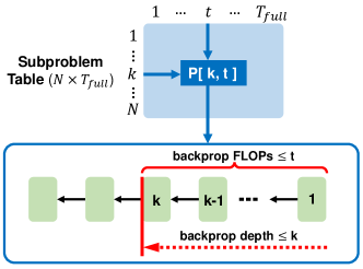
(a) Subproblem definition

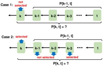
(b) Finding recurrence relations

Figure 4: Solving the selection problem by DP

Recurrence relations of subproblems. The recurrence relation between subproblem $P[k,t]$ and $P[k-1,t]$ depends on whether we further select the top tensor $k$ from the solution of $P[k-1,t]$, as shown in Figure 4(b). Case 1: If the top tensor $k$ is not selected, $P[k,t]$ will fall back to $P[k-1,t]$, since the importance of selected tensors will not be further increased. Case 2: If the top tensor $k$ is selected, then its FLOPs will be included into the solution of $P[k,t]$, no matter which other tensors are selected. The FLOPs involved with tensor $k$ include 1) the FLOPs to update tensor $k$ and 2) the FLOPs to pass activation gradients from the closest selected tensor $k_{c}$, such as tensor $k-3$ as shown in Figure 4(b), to tensor $k$. This implies that $P[k,t]$ falls back to a previously solved subproblem $P[k-k_{c},t-\Delta t]$, where

$$\Delta t=t_{dw_{k}}+\sum\nolimits_{j=k_{c}}^{k-1}t_{dy_{j}}.$$ (12)

Since $k_{c}$ is unknown in advance, we backtrace the previously solved subproblems and explore all the possibilities of $k_{c}$ by reducing the depth of backpropagation from $k$, and the optimal solution to $P[k,t]$ is the one with the highest cumulative importance of the selected tensors. Based on this recurrence relation, we can solve all the subproblems by sequentially traversing the subproblem space. The time complexity of solving each subproblem is $O(N)$ due to the backtracing in Case 2, and the overall time complexity of DP algorithm is $O(N^{2}T_{full})$.

Reducing the computational cost. Due to the high volume of FLOPs in LLM fine-tuning, the value of $T_{full}$ could be very large. To reduce the computational cost of DP, we can reduce the subproblem space by skipping two types of subproblems: 1) invalid ones, whose FLOPs constraint $t$ exceeds the desired constraint ($\rho T_{full}$); 2) redundant ones, whose FLOPs to pass activation gradients to the maximally allowed depth ($k$) exceeds $t$. Our preliminary experiment show that, doing so on an OPT model with $\rho_{bp}=50\%$ can reduce the number of subproblems by 5.5$\times$ without affecting the optimality of training.

Besides, to further reduce the number of subproblems, we scale tensors’ FLOPs $({t_{dw}},{t_{dy}})$ by multiplying a factor of $Z$:

$$\widetilde{t_{dw}}=\left\lfloor t_{dw}\cdot{Z}\right\rfloor,\ \ \ \ \widetilde{t_{dy}}=\left\lfloor t_{dy}\cdot{Z}\right\rfloor,\ \ \ \$$ (13)

where $Z=\frac{T_{q}}{T_{full}}$ reduces the backropagation FLOPs to a resolution of $T_{q}<T_{full}$. The overall time complexity of DP is then reduced to $O(N^{2}T_{q})$. On the other hand, such reduced resolution could increase the ambiguity in DP and affect the training quality. To investigate such tradeoff between the training quality and cost, we conducted preliminary experiments on multiple LLMs. Results in Table 3 show that, for both OPT-2.7B and BLOOMZ-3B models, setting $T_{q}=1e3$ reduces the DP overhead to $<1$% without affecting the training quality. Similarly, for FLAN-T5-3B, choosing $T_{q}=1e2$ can retain good training quality with negligible overhead. On the other hand, when $T_{q}$ is too small, the solution of DP could be inaccurate and hence result in ineffective reduction of the training FLOPs.

Model	$T_{q}=1e1$	$T_{q}=1e2$	$T_{q}=1e3$	$T_{q}=1e4$	$T_{q}=1e5$
OPT-2.7B	0.02/64.1/32.0	0.04/47.6/30.1	0.64/49.8/30.7	7.5/50.0/30.9	76.5/50.0/30.9
BLOOMZ-3B	0.0001/33.3/9.30	0.007/45.7/25.2	0.21/49.5/27.2	2.3/49.8/27.1	25.3/50.0/27.1
FLAN-T5-3B	0.04/64.9/36.5	0.25/57.1/36.5	3.5/55.3/36.7	41.8/51.8/36.7	449/50.0/36.7

Table 3: The impact of DP resolution $T_{q}$ on fine-tuning OPT-2.7B, BLOOMZ-3B, and FLAN-T5-3B LLMs, on the SciTLDR dataset with $\rho=50\%$. Each triplet [a/b/c] presents a) the percentage of wall-clock time incurred by DP compared to full fine-tuning, b) the percentage of FLOPs after reduction compared to full fine-tuning, and c) the testing ROUGE-1 score, respectively.

4 Experiments

We implemented GreenTrainer in PyTorch and conducted our experiments on a Lambda Cloud instance with a Nvidia H100 80GB GPU and 24 vCPUs. In our evaluation, we include recently open-sourced decoder-only LLMs including OPT [44] and BLOOMZ [30], and an encoder-decoder LLM, namely FLAN-T5 [10]). The number of parameters in these LLMs ranges from 350M to 6.7B, depending on the specific model variants. Our experiments are conducted using the following two datasets of abstractive summarization:

• SciTLDR [7] is a dataset of 5.4K text summaries over 3.2K papers. It contains both author-written and expert-derived TLDRs, where the latter ones are collected using a novel annotation protocol that produces high-quality summaries while minimizing the annotation burden.

• DialogSum [9] is a dialogue summarization dataset, consisting of 13,460 dialogues with corresponding manually labeled summaries and topics. It has been demonstrated more challenging than other summarization datasets, such as SAMSum [13] and CNN/Daily [31] at a similar scale.

Note that, in our evaluations we do not consider non-generative tasks such as sentimental classification, entailment classification, and extractive QA. The basic reason is that these tasks are too easy for today’s LLMs, and testing them with LLMs will hence result in exaggerated performance gain over the baseline.

For OPT and BLOOMZ, we follow GPT2-like prompt structures [34], “[source seq.] TL;DR:”, for summarization tasks to preprocess all the input data. For FLAN-T5, we adopt the prompt structure “summarize: [source seq.]”, which is used in the original T5 pre-training. We truncate the source sequences so that the length of every preprocessed input sequence is within 512 tokens. On the test data, we use a beam search size of 4, and set the maximum number of generated tokens to 64 for SciTLDR and 128 for DialogSum. We compare the performance of GreenTrainer (GT) with the following four baselines:

• Full Fine-Tuning (Full FT) fine-tunes all the LLM parameters and should intuitively achieve the best accuracy of the trained model.

• Fine-Tuning Top2 (FT-Top2) only fine-tunes the last two layers of the LLM, which typically include the embedding layer and a LayerNorm. The input and output embedding layers are tied for OPT and BLOOMZ, but are not tied for FLAN-T5. This naive baseline only fine-tunes the smallest portion of LLM parameters and is used to identify whether the dataset is trivial to the LLM.

• Prefix Tuning (Prefix-T) [23] inserts trainable prefixes into each transformer block’s input sequence while freezing the model parameters. For encoder-decoder LLMs, the trainable prefixes are only inserted into the decoder blocks.

• LoRA [16] is currently the most popular method for efficient LLM fine-tuning. It uses low-rank matrix decomposition to reduce the training cost. We apply LoRA to both query and value projectors, as suggested in [16].

In all experiments, we use a batch size of 4 and fine-tune the model for 5 epochs. We use the AdamW optimizer [27] at a learning rate of $2\times 10^{-5}$ with linear schedule and weight decay of $10^{-2}$. We use the ROUGE scores (%R1/R2/RL) [25] on the test datasets as the accuracy metric, and measure both the Peta-FLOPs (PFLOPs) and wall-clock time as the training cost in each run.

# Model & Method	SciTLDR			DialogSum
	PFLOPs	Time (h)	R1/R2/RL	PFLOPs	Time (h)	R1/R2/RL
OPT-2.7B
Full FT	41.8	0.92	32.9/14.9/27.1	262.0	5.5	23.6/9.5/18.8
FT-Top2	29.0 (31%$\downarrow$)	0.61 (34%$\downarrow$)	9.1/4.0/7.6	181.6 (31%$\downarrow$)	3.8 (31%$\downarrow$)	20.8/7.9/17.5
Prefix-T	27.9 (33%$\downarrow$)	0.58 (37%$\downarrow$)	7.6/0.4/6.1	174.7 (33%$\downarrow$)	3.7 (33%$\downarrow$)	13.4/3.3/10.9
LoRA	27.9 (33%$\downarrow$)	0.59 (36%$\downarrow$)	28.2/12.1/21.0	174.7 (33%$\downarrow$)	3.6 (35%$\downarrow$)	23.8/9.5/18.8
GT-0.5	20.8 (50%$\downarrow$)	0.46 (50%$\downarrow$)	30.5/13.1/25.2	130.1 (50%$\downarrow$)	2.7 (51%$\downarrow$)	21.4/8.2/17.6
GT-0.7	29.2 (30%$\downarrow$)	0.68 (26%$\downarrow$)	33.1/15.2/27.6	182.7 (30%$\downarrow$)	4.0 (27%$\downarrow$)	26.8/11.0/21.6
BLOOMZ-3B
Full FT	47.2	1.0	28.3/12.1/22.5	294.8	6.5	26.1/10.6/21.0
FT-Top2	36.5 (23%$\downarrow$)	0.75 (25%$\downarrow$)	23.7/8.8/18.8	227.9 (23%$\downarrow$)	4.6 (29%$\downarrow$)	22.1/8.5/17.8
Prefix-T	31.5 (33%$\downarrow$)	0.68 (34%$\downarrow$)	6.5/2.2/5.5	196.5 (33%$\downarrow$)	4.2 (35%$\downarrow$)	29.6/9.4/24.9
LoRA	31.5 (33%$\downarrow$)	0.69 (33%$\downarrow$)	27.4/11.7/21.8	196.5 (33%$\downarrow$)	4.3 (34%$\downarrow$)	35.4/14.3/28.6
GT-0.5	23.4 (51%$\downarrow$)	0.51 (50%$\downarrow$)	26.7/10.7/21.2	146.4 (50%$\downarrow$)	3.1 (52%$\downarrow$)	24.9/9.5/20.0
GT-0.7	32.3 (32%$\downarrow$)	0.74 (28%$\downarrow$)	28.0/12.2/22.4	204.7 (31%$\downarrow$)	4.3 (34%$\downarrow$)	36.8/14.7/29.4
FLAN-T5-3B
Full FT	21.7	0.64	37.1/18.5/31.7	135.7	4.0	46.5/20.8/38.5
FT-Top2	7.3 (66%$\downarrow$)	0.21 (67%$\downarrow$)	36.5/18.4/31.5	46.1 (66%$\downarrow$)	1.4 (65%$\downarrow$)	39.2/16.7/32.9
Prefix-T	8.0 (63%$\downarrow$)	0.23 (64%$\downarrow$)	36.0/18.2/31.0	55.3 (60%$\downarrow$)	1.7 (57%$\downarrow$)	37.6/16.4/32.1
LoRA	14.4 (33%$\downarrow$)	0.41 (36%$\downarrow$)	36.6/18.5/31.5	90.5 (33%$\downarrow$)	2.5 (38%$\downarrow$)	44.7/19.8/37.1
GT-0.34	7.5 (65%$\downarrow$)	0.23 (64%$\downarrow$)	36.4/18.4/31.7	53.5 (61%$\downarrow$)	1.4 (65%$\downarrow$)	42.7/18.3/35.1
GT-0.4	10.0 (54%$\downarrow$)	0.38 (41%$\downarrow$)	36.7/18.5/31.5	62.5 (54%$\downarrow$)	2.3 (43%$\downarrow$)	46.0/20.7/38.1
GT-0.5	12.4 (43%$\downarrow$)	0.44 (31%$\downarrow$)	36.3/17.7/30.9	77.6 (43%$\downarrow$)	2.6 (35%$\downarrow$)	46.2/20.7/38.1

Table 4: Comparison of the training cost & accuracy in LLM fine-tuning. GreenTrainer with an objective $\rho$ of FLOPs reduction is denoted as GT-$\rho$.

4.1 Training Cost & Accuracy

We first compare the training cost and accuracy of GreenTrainer (GT) with other baseline schemes on LLMs with 3B parameters, using both datasets. As shown in Table 4, for the OPT-2.7B model, GT-0.5 can achieve the required objective of FLOPs reduction (50%), with at most 2% accuracy loss on both datasets, and GT-0.7 can even achieve 0.2%-3% higher ROUGE scores than Full FT. We hypothesize that GT achieves such accuracy improvement by only fine-tuning the most important tensors and hence mitigating the overfitting that may exist in Full FT. On the other hand, insufficient trainable parameters can also lead to underfitting, such that FT-Top2 has significantly lower ROUGE scores than all other schemes, indicating that the fine-tuning task is non-trivial for the OPT-2.7B model. Similarly, compared to LoRA and Prefix Tuning, GT-0.7 achieves at least 2% higher accuracy with the same amount of training FLOPs.

Similarly, for BLOOMZ-3B, GT-0.5 can save 50% training FLOPs and wall-clock time with $<2$% accuracy loss. Compared to Full FT, GT-0.7 achieves the same ROUGE scores on the SciTLDR dataset, and 4% to 10% higher on the DialogSum dataset. With the same training FLOPs, GT-0.7 has 0.4%-1.4% higher ROUGE scores than the best baseline (LoRA). Note that both datasets are non-trivial for the BLOOMZ model, since the naive baseline (FT-Top2) still exhibits significant accuracy loss, and Prefix-T performs much worse than any other baselines on the SciTLDR dataset. The major reason may be that the inserted trainable prefixes break the original prompt structure and confuse the model on the scientific corpus.

For the FLAN-T5-3B model, we observe that FT-Top2 achieves similar fine-tuning qualities to Full FT with significant FLOPs reduction, indicating that the SciTLDR dataset is trivial for FLAN-T5. This is because FLAN-T5 has been instruction-fine-tuned after pre-training, and can potentially have better zero-shot adaptability. In this case, GT-0.34 can achieve the same training FLOPs and ROUGE scores by selecting only a small portion of tensors. On the other hand, FT-Top2 loses accuracy significantly on the DialogSum dataset, but GT-0.4 reduces 54% of training FLOPs and 43% of wall-clock time without noticeable accuracy loss. GT-0.4 also outperforms LoRA by 1% on ROUGE scores and reduces 11% more training FLOPs. Compared to Prefix tuning, GT-0.34 achieves 2%-5% higher ROUGE scores, while reducing the same amount of training FLOPs.

4.2 The Impact of FLOPs Reduction Objective

To better understand how GreenTrainer performs with different objectives of FLOPs reduction, we vary the value of $\rho$ between 0.36 and 0.8, and compare GreenTrainer with LoRA, which provides the best training performance among all the baseline schemes, on the OPT-2.7B model. As shown in Table 5, on the SciTLDR dataset, when the requirement of FLOPs reduction is high and corresponds to a value of $\rho\leq$0.4, GreenTrainer outperforms LoRA by achieving 2% higher ROUGE scores and saving 25% more FLOPs and wall-clock time. On the other hand, when the value of $\rho$ increases to 0.6, GreenTrainer outperforms the Full FT on ROUGE scores by 0.5% and outperforms LoRA by 5.2%, but saves 40% of training FLOPs and 39% of wall-clock time compared to Full FT. Similar results are also observed on the DialogSum dataset. In summary, with different objectives of FLOPs reduction, GreenTrainer can always provide better tradeoffs between the training accuracy and cost, compared to the SOTA baselines.

Method	SciTLDR			DialogSum
	PFLOPs	Time (h)	R1/R2/RL	PFLOPs	Time (h)	R1/R2/RL
Full FT	41.8	0.92	32.9/14.9/27.1	262.0	5.5	23.6/9.5/18.8
LoRA	27.9 (33%$\downarrow$)	0.59 (36%$\downarrow$)	28.2/12.1/21.0	174.7 (33%$\downarrow$)	3.6 (35%$\downarrow$)	23.8/9.5/18.8
GT-0.36	14.9 (64%$\downarrow$)	0.32 (65%$\downarrow$)	4.1/1.7/3.6	92.9 (65%$\downarrow$)	1.9 (65%$\downarrow$)	15.7/5.0/13.8
GT-0.4	16.6 (60%$\downarrow$)	0.36 (61%$\downarrow$)	28.6/11.6/23.5	103.4 (61%$\downarrow$)	2.2 (60%$\downarrow$)	17.9/6.3/15.4
GT-0.5	20.8 (50%$\downarrow$)	0.46 (50%$\downarrow$)	30.5/13.1/25.2	130.1 (50%$\downarrow$)	2.7 (51%$\downarrow$)	21.4/8.2/17.6
GT-0.6	25.0 (40%$\downarrow$)	0.56 (39%$\downarrow$)	33.4/15.3/27.8	156.6 (40%$\downarrow$)	3.3 (40%$\downarrow$)	24.0/9.7/19.2
GT-0.7	29.2 (30%$\downarrow$)	0.68 (26%$\downarrow$)	33.1/15.2/27.6	182.7 (30%$\downarrow$)	4.0 (27%$\downarrow$)	26.8/11.0/21.6
GT-0.8	33.4 (20%$\downarrow$)	0.77 (16%$\downarrow$)	33.1/15.5/27.6	209.6 (20%$\downarrow$)	4.4 (20%$\downarrow$)	23.9/9.9/19.1

Table 5: Impact of different objectives of FLOPs reduction on the OPT-2.7B model

These results, on the other hand, also demonstrates that GreenTrainer provides great flexibility in LLM fine-tuning between the training accuracy and cost, by adjusting the value of $\rho$. The user can opt to set a low value of $\rho$ ($\leq$0.4) to maximize the FLOPs reduction ($>$60%) with moderate model accuracy loss (3%-4% on the two datasets we use). Alternatively, they can use a high value of $\rho$ ($\geq$0.6) to have the same level of FLOPs reduction as that of LoRA, but ensure the minimum model accuracy loss or even minor model accuracy improvement. We believe that such flexibility is practically important when fine-tuning LLMs for downstream tasks with different green AI requirements and constraints.

4.3 Efficacy of Tensor Importance Metrics

The fine-tuning quality of GreenTrainer builds on the effectiveness of tensor importance evaluation. We compare our metric ($\Delta w\frac{\partial L}{\partial w}$) to the magnitude-based metric ($\Delta w$) [20] and the gradients-only metric ($\frac{\partial L}{\partial w}$) [3], using the OPT-2.7B model with $\rho=$0.7. As shown in Table 6, with the same objective of FLOPs reduction, using our metric ($\Delta w\frac{\partial L}{\partial w}$) for tensor importance evaluation achieves the highest model accuracy and outperforms Full FT by 1%-3% on ROUGE scores. This is because magnitude-based metrics ignore the dependencies of weight updates. Gradient-only metrics, on the other hand, only contain the direction information about tensor importance but cannot reflect the intensity of importance. Inaccurate importance measurements will in turn lead to inappropriate selections of trainable tensors.

Method	SciTLDR			DialogSum
	PFLOPs	Time (h)	R1/R2/RL	PFLOPs	Time (h)	R1/R2/RL
Full FT	41.8	0.92	32.9/14.9/27.1	262.0	5.5	23.6/9.5/18.8
GT-0.7 ($\Delta w$)	29.4 (30%$\downarrow$)	0.68 (26%$\downarrow$)	32.7/15.2/27.2	183.8 (30%$\downarrow$)	4.0 (27%$\downarrow$)	24.9/10.2/19.7
GT-0.7 ($\frac{\partial L}{\partial w}$)	29.4 (30%$\downarrow$)	0.67 (27%$\downarrow$)	32.8/15.1/27.2	184.0 (30%$\downarrow$)	4.0 (27%$\downarrow$)	25.0/10.2/20.0
GT-0.7 ($\Delta w\frac{\partial L}{\partial w}$)	29.2 (30%$\downarrow$)	0.68 (26%$\downarrow$)	33.1/15.2/27.6	182.7 (30%$\downarrow$)	4.0 (27%$\downarrow$)	26.8/11.0/21.6

Table 6: Efficacy of Tensor Importance Metrics (OPT-2.7B)

4.4 Impact of LLM Size

A specific type of LLM may contain several variants with different parameter sizes. To study GreenTrainer’s performance with different LLM sizes, we performed LLM fine-tuning using the OPT models with parameter sizes, ranging from 350M to 6.7B. As shown in Table 7, even on small models (OPT-350M), GT-0.5 can save 17%-21% more training FLOPs than LoRA does, while achieving 2%-4% higher accuracy (on SciTDR) or the same accuracy (on DialogSum). When the model size increases to 2.7B, GT-0.5 outperforms LoRA and GT-0.7 outperforms Full FT on the SciTLDR dataset. On DialogSum, GT-0.7 performs similarly compared to LoRA. For the OPT-6.7B model, GT-0.4 can save 27% more training FLOPs than LoRA does on SciTLDR, while achieving the same model accuracy, and similar advantages can also be observed when comparing GT-0.5 and GT-0.7 with LoRA. Generally speaking, GreenTrainer’s performance advantage widely applies to LLMs with different sizes.

# Params & Method	SciTLDR			DialogSum
	PFLOPs	Time (h)	R1/R2/RL	PFLOPs	Time (h)	R1/R2/RL
OPT-350M
Full FT	5.4	0.15	30.9/13.9/25.7	33.8	0.92	23.2/9.0/18.5
LoRA	3.6 (33%$\downarrow$)	0.10 (33%$\downarrow$)	25.9/10.8/20.3	22.5 (33%$\downarrow$)	0.65 (29%$\downarrow$)	21.5/7.7/17.3
GT-0.4	2.1 (61%$\downarrow$)	0.06 (60%$\downarrow$)	27.7/12.2/23.4	13.3 (61%$\downarrow$)	0.36 (61%$\downarrow$)	17.3/5.8/14.6
GT-0.5	2.7 (50%$\downarrow$)	0.08 (47%$\downarrow$)	29.9/13.2/24.9	16.7 (51%$\downarrow$)	0.45 (51%$\downarrow$)	21.3/7.8/17.3
GT-0.7	3.8 (30%$\downarrow$)	0.12 (20%$\downarrow$)	30.6/13.5/25.0	23.6 (30%$\downarrow$)	0.66 (28%$\downarrow$)	24.2/9.3/19.3
OPT-1.3B
Full FT	20.8	0.46	32.1/14.3/26.4	130.8	2.9	25.4/10.3/20.2
LoRA	13.9 (33%$\downarrow$)	0.31 (33%$\downarrow$)	28.1/11.9/22.0	87.2 (33%$\downarrow$)	1.9 (34%$\downarrow$)	24.6/9.9/19.4
GT-0.4	8.2 (61%$\downarrow$)	0.18 (61%$\downarrow$)	28.9/11.9/23.8	51.4 (61%$\downarrow$)	1.1 (62%$\downarrow$)	16.9/5.7/14.6
GT-0.5	10.3 (50%$\downarrow$)	0.23 (50%$\downarrow$)	30.0/12.7/24.5	64.2 (51%$\downarrow$)	1.4 (51%$\downarrow$)	20.1/7.4/16.7
GT-0.7	14.5 (30%$\downarrow$)	0.34 (26%$\downarrow$)	31.2/14.2/25.8	90.8 (30%$\downarrow$)	2.0 (31%$\downarrow$)	24.4/9.7/19.4
OPT-2.7B
Full FT	41.8	0.92	32.9/14.9/27.1	262.0	5.5	23.6/9.5/18.8
LoRA	27.9 (33%$\downarrow$)	0.59 (36%$\downarrow$)	28.2/12.1/21.0	174.7 (33%$\downarrow$)	3.6 (35%$\downarrow$)	23.8/9.5/18.8
GT-0.4	16.6 (60%$\downarrow$)	0.36 (61%$\downarrow$)	28.6/11.6/23.5	103.4 (61%$\downarrow$)	2.2 (60%$\downarrow$)	17.9/6.3/15.4
GT-0.5	20.8 (50%$\downarrow$)	0.46 (50%$\downarrow$)	30.5/13.1/25.2	130.1 (50%$\downarrow$)	2.7 (51%$\downarrow$)	21.4/8.2/17.6
GT-0.7	29.2(30%$\downarrow$)	0.68 (26%$\downarrow$)	33.1/15.2/27.6	182.7 (30%$\downarrow$)	4.0 (27%$\downarrow$)	26.8/11.0/21.6
OPT-6.7B
Full FT	103.9	5.44	32.9/14.9/27.5	649.9	-	-
LoRA	69.3 (33%$\downarrow$)	1.3	28.4/12.3/22.7	433.3 (33%$\downarrow$)	8.1	24.9/10.2/19.4
GT-0.4	41.2 (60%$\downarrow$)	0.9	28.9/11.8/23.4	257.9 (60%$\downarrow$)	5.2	19.7/7.0/16.3
GT-0.5	50.8 (51%$\downarrow$)	1.1	30.1/13.0/24.8	331.4 (49%$\downarrow$)	6.7	21.8/8.5/17.3
GT-0.7	74.8 (28%$\downarrow$)	1.4	33.1/15.3/27.7	-	-	-

Table 7: Impact of LLM’s model size

5 Conclusion & Broader Impact

In this paper, we present GreenTrainer, a new fine-tuning technique for LLMs that allows efficient selection of trainable parameters via adaptive backpropagation, to ensure high training quality while significantly reducing the computation cost. GreenTrainer can save up to 64% training FLOPs compared to full fine-tuning without noticeable accuracy loss. Compared to the existing fine-tuning technique such as Prefix Tuning and LoRA, GreenTrainer can achieve up to 4% accuracy improvement with the same amount of FLOPs reduction.

Although we target LLM fine-tuning in this paper, the rationale of GreenTrainer’s adaptive backpropagation can also be applicable to large generative models in other fields, such as Stable Diffusion [35] for image generation and PaLM-E [12] for motion planning of multimodal embodied agents. Extensions to these domains will be our future work.

References

- aii [2023] 2023 ai index report. https://aiindex.stanford.edu/report/, 2023.
- Abadi [2016] M. Abadi. Tensorflow: learning functions at scale. In Proceedings of the 21st ACM SIGPLAN International Conference on Functional Programming, pages 1–1, 2016.
- Aji and Heafield [2017] A. F. Aji and K. Heafield. Sparse communication for distributed gradient descent. arXiv preprint arXiv:1704.05021, 2017.
- Ba et al. [2016] J. L. Ba, J. R. Kiros, and G. E. Hinton. Layer normalization. arXiv preprint arXiv:1607.06450, 2016.
- Breiman [2001] L. Breiman. Random forests. Machine learning, 45:5–32, 2001.
- Brown et al. [2020] T. Brown, B. Mann, N. Ryder, M. Subbiah, J. D. Kaplan, P. Dhariwal, A. Neelakantan, P. Shyam, G. Sastry, A. Askell, et al. Language models are few-shot learners. Advances in neural information processing systems, 33:1877–1901, 2020.
- Cachola et al. [2020] I. Cachola, K. Lo, A. Cohan, and D. S. Weld. Tldr: Extreme summarization of scientific documents. arXiv preprint arXiv:2004.15011, 2020.
- Candel et al. [2023] A. Candel, J. McKinney, P. Singer, P. Pfeiffer, M. Jeblick, P. Prabhu, J. Gambera, M. Landry, S. Bansal, R. Chesler, et al. h2ogpt: Democratizing large language models. arXiv preprint arXiv:2306.08161, 2023.
- Chen et al. [2021] Y. Chen, Y. Liu, L. Chen, and Y. Zhang. Dialogsum: A real-life scenario dialogue summarization dataset. arXiv preprint arXiv:2105.06762, 2021.
- Chung et al. [2022] H. W. Chung, L. Hou, S. Longpre, B. Zoph, Y. Tay, W. Fedus, E. Li, X. Wang, M. Dehghani, S. Brahma, et al. Scaling instruction-finetuned language models. arXiv preprint arXiv:2210.11416, 2022.
- Devlin et al. [2018] J. Devlin, M.-W. Chang, K. Lee, and K. Toutanova. Bert: Pre-training of deep bidirectional transformers for language understanding. arXiv preprint arXiv:1810.04805, 2018.
- Driess et al. [2023] D. Driess, F. Xia, M. S. Sajjadi, C. Lynch, A. Chowdhery, B. Ichter, A. Wahid, J. Tompson, Q. Vuong, T. Yu, et al. Palm-e: An embodied multimodal language model. arXiv preprint arXiv:2303.03378, 2023.
- Gliwa et al. [2019] B. Gliwa, I. Mochol, M. Biesek, and A. Wawer. Samsum corpus: A human-annotated dialogue dataset for abstractive summarization. arXiv preprint arXiv:1911.12237, 2019.
- Guo et al. [2020] Y. Guo, Y. Li, L. Wang, and T. Rosing. Adafilter: Adaptive filter fine-tuning for deep transfer learning. In Proceedings of the AAAI Conference on Artificial Intelligence, volume 34, pages 4060–4066, 2020.
- Hesse et al. [2021] R. Hesse, S. Schaub-Meyer, and S. Roth. Fast axiomatic attribution for neural networks. Advances in Neural Information Processing Systems, 34:19513–19524, 2021.
- Hu et al. [2021] E. J. Hu, Y. Shen, P. Wallis, Z. Allen-Zhu, Y. Li, S. Wang, L. Wang, and W. Chen. Lora: Low-rank adaptation of large language models. arXiv preprint arXiv:2106.09685, 2021.
- Hu et al. [2023] Z. Hu, Y. Lan, L. Wang, W. Xu, E.-P. Lim, R. K.-W. Lee, L. Bing, and S. Poria. Llm-adapters: An adapter family for parameter-efficient fine-tuning of large language models. arXiv preprint arXiv:2304.01933, 2023.
- Jin et al. [2020] G. Jin, X. Yi, L. Zhang, L. Zhang, S. Schewe, and X. Huang. How does weight correlation affect generalisation ability of deep neural networks? Advances in Neural Information Processing Systems, 33:21346–21356, 2020.
- Lamb et al. [2016] A. M. Lamb, A. G. ALIAS PARTH GOYAL, Y. Zhang, S. Zhang, A. C. Courville, and Y. Bengio. Professor forcing: A new algorithm for training recurrent networks. Advances in neural information processing systems, 29, 2016.
- Lee et al. [2020] J. Lee, S. Park, S. Mo, S. Ahn, and J. Shin. Layer-adaptive sparsity for the magnitude-based pruning. arXiv preprint arXiv:2010.07611, 2020.
- Lester et al. [2021] B. Lester, R. Al-Rfou, and N. Constant. The power of scale for parameter-efficient prompt tuning. arXiv preprint arXiv:2104.08691, 2021.
- Li et al. [2016] H. Li, A. Kadav, I. Durdanovic, H. Samet, and H. P. Graf. Pruning filters for efficient convnets. arXiv preprint arXiv:1608.08710, 2016.
- Li and Liang [2021] X. L. Li and P. Liang. Prefix-tuning: Optimizing continuous prompts for generation. arXiv preprint arXiv:2101.00190, 2021.
- Liao et al. [2023] B. Liao, S. Tan, and C. Monz. Make your pre-trained model reversible: From parameter to memory efficient fine-tuning. arXiv preprint arXiv:2306.00477, 2023.
- Lin [2004] C.-Y. Lin. ROUGE: A package for automatic evaluation of summaries. In Text Summarization Branches Out, pages 74–81, Barcelona, Spain, July 2004. Association for Computational Linguistics. URL https://www.aclweb.org/anthology/W04-1013.
- Liu et al. [2022] X. Liu, K. Ji, Y. Fu, W. Tam, Z. Du, Z. Yang, and J. Tang. P-tuning: Prompt tuning can be comparable to fine-tuning across scales and tasks. In Proceedings of the 60th Annual Meeting of the Association for Computational Linguistics (Volume 2: Short Papers), pages 61–68, 2022.
- Loshchilov and Hutter [2017] I. Loshchilov and F. Hutter. Decoupled weight decay regularization. arXiv preprint arXiv:1711.05101, 2017.
- Lu et al. [2021] K. Lu, A. Grover, P. Abbeel, and I. Mordatch. Pretrained transformers as universal computation engines. arXiv preprint arXiv:2103.05247, 1, 2021.
- Malladi et al. [2023] S. Malladi, T. Gao, E. Nichani, A. Damian, J. D. Lee, D. Chen, and S. Arora. Fine-tuning language models with just forward passes. arXiv preprint arXiv:2305.17333, 2023.
- Muennighoff et al. [2022] N. Muennighoff, T. Wang, L. Sutawika, A. Roberts, S. Biderman, T. L. Scao, M. S. Bari, S. Shen, Z.-X. Yong, H. Schoelkopf, et al. Crosslingual generalization through multitask finetuning. arXiv preprint arXiv:2211.01786, 2022.
- Nallapati et al. [2016] R. Nallapati, B. Zhou, C. Gulcehre, B. Xiang, et al. Abstractive text summarization using sequence-to-sequence rnns and beyond. arXiv preprint arXiv:1602.06023, 2016.
- Ott et al. [2019] M. Ott, S. Edunov, A. Baevski, A. Fan, S. Gross, N. Ng, D. Grangier, and M. Auli. fairseq: A fast, extensible toolkit for sequence modeling. arXiv preprint arXiv:1904.01038, 2019.
- Paszke et al. [2019] A. Paszke, S. Gross, F. Massa, A. Lerer, J. Bradbury, G. Chanan, T. Killeen, Z. Lin, N. Gimelshein, L. Antiga, et al. Pytorch: An imperative style, high-performance deep learning library. Advances in neural information processing systems, 32, 2019.
- Radford et al. [2019] A. Radford, J. Wu, R. Child, D. Luan, D. Amodei, I. Sutskever, et al. Language models are unsupervised multitask learners. OpenAI blog, 1(8):9, 2019.
- Rombach et al. [2022] R. Rombach, A. Blattmann, D. Lorenz, P. Esser, and B. Ommer. High-resolution image synthesis with latent diffusion models. In Proceedings of the IEEE/CVF Conference on Computer Vision and Pattern Recognition, pages 10684–10695, 2022.
- Schwartz et al. [2020] R. Schwartz, J. Dodge, N. A. Smith, and O. Etzioni. Green ai. Communications of the ACM, 63(12):54–63, 2020.
- Scialom et al. [2022] T. Scialom, T. Chakrabarty, and S. Muresan. Fine-tuned language models are continual learners. In Proceedings of the 2022 Conference on Empirical Methods in Natural Language Processing, pages 6107–6122, 2022.
- Sundararajan et al. [2017] M. Sundararajan, A. Taly, and Q. Yan. Axiomatic attribution for deep networks. In International conference on machine learning, pages 3319–3328. PMLR, 2017.
- Touvron et al. [2023] H. Touvron, T. Lavril, G. Izacard, X. Martinet, M.-A. Lachaux, T. Lacroix, B. Rozière, N. Goyal, E. Hambro, F. Azhar, et al. Llama: Open and efficient foundation language models. arXiv preprint arXiv:2302.13971, 2023.
- Vaswani et al. [2017] A. Vaswani, N. Shazeer, N. Parmar, J. Uszkoreit, L. Jones, A. N. Gomez, Ł. Kaiser, and I. Polosukhin. Attention is all you need. Advances in neural information processing systems, 30, 2017.
- Wolf et al. [2019] T. Wolf, L. Debut, V. Sanh, J. Chaumond, C. Delangue, A. Moi, P. Cistac, T. Rault, R. Louf, M. Funtowicz, et al. Huggingface’s transformers: State-of-the-art natural language processing. arXiv preprint arXiv:1910.03771, 2019.
- Zaken et al. [2021] E. B. Zaken, S. Ravfogel, and Y. Goldberg. Bitfit: Simple parameter-efficient fine-tuning for transformer-based masked language-models. arXiv preprint arXiv:2106.10199, 2021.
- Zhang et al. [2023] Q. Zhang, M. Chen, A. Bukharin, P. He, Y. Cheng, W. Chen, and T. Zhao. Adaptive budget allocation for parameter-efficient fine-tuning. arXiv preprint arXiv:2303.10512, 2023.
- Zhang et al. [2022] S. Zhang, S. Roller, N. Goyal, M. Artetxe, M. Chen, S. Chen, C. Dewan, M. Diab, X. Li, X. V. Lin, et al. Opt: Open pre-trained transformer language models. arXiv preprint arXiv:2205.01068, 2022.