Statistical Hypothesis Testing for Information Value (IV)

Abstract

Information value (IV) is a quite popular technique for features selection before the modeling phase. There are practical criteria, based on fixed thresholds for IV, but at the same time mysterious and lacking theoretical arguments, to decide if a predictor has sufficient predictive power to be considered in the modeling phase. However, the mathematical development and statistical inference methods for this technique are almost nonexistent in the literature. In this paper we present a theoretical framework for IV, and at the same time, we propose a non-parametric hypothesis test to evaluate the predictive power of features contemplated in a data set. Due to its relationship with divergence measures developed in the Information Theory, we call our proposal the J - Divergence test. We show how to efficiently compute our test statistic and we study its performance on simulated data. In various scenarios, particularly in unbalanced data sets, we show its superiority over conventional criteria based on fixed thresholds. Furthermore, we apply our test on fraud identification data and provide an open-source Python library, called “statistical-iv”, where we implement our main results.

Keywords: Information Value (IV), Weight of Evidence (WoE), Jeffreys Divergence, Features Selection, Central Limit Theorem.

1 Introduction

Feature selection in classification problems, or also known as predictor variable reduction, is an important step before venturing to build a model. In high-dimensional data, data sets with many features, this is even more important, because parsimonious and easy-to-interpret models are prioritized. Information Value (IV) is a quite popular tool for features selection in binary classification problems. Initially, the IV, in conjunction with Weight of Evidence (WoE), inspired by Information Theory developed in the 1940s [1; 2], was designed to selection, raking and monitor predictor variables in the credit risk industry [9]. However, in recent years it has received increasing attention in diverse areas such as; marketing, engineering and geosciences [3; 5; 4]. In machine learning, in a very useful and interesting way, IV is used to the optimal discretization of a variable into bins given a discrete or continuous numeric target, process known as optimal binning [6]. Furthermore, the implementation using the IV is simple and practical [7; 8].

In order to illustrate how the IV is calculated, consider a binary target $y$ and $x$ a feature for which we want to evaluate its predictive power. The predictor variable $x$ is organized in $r$ bins (groups or buckets). For binning techniques in detail, see [6]. Let $g_{j}$ the count of instances with $y=1$ at bin $j$, and $g_{t}$ the count of total instances with $y=1$. Define the empirical relative frequencies $\hat{p}_{j}$ for each bin $j$ as $\hat{p}_{j}=\frac{g_{j}}{g_{t}}$. Correspondingly, define the empirical relative frequencies $\hat{q}_{j}=\frac{b_{j}}{b_{t}}$ for each bin $j$, where $b_{j}$ the count of instances with $y=0$ at bin $j$, and $b_{t}$ the count of total instances with $y=0$. Then, the Weight of Evidence (WoE) for bin $j$ is defined as

IV	Predictive Power
<0.02	Not useful for prediction
0.02 to 0.1	Weak
0.1 to 0.3	Medium
0.3 to 0.5	Strong
>0.5	Suspicious Predictive Power

Table 1: Threshold values for IV [9].

$$\textrm{WoE}_{j}=\ln\Big{(}\frac{\hat{p}_{j}}{\hat{q}_{j}}\Big{)},$$

and IV of predictor $x$ is defined by

$$\textrm{IV}=\sum\limits_{j=1}^{r}(\hat{p}_{j}-\hat{p}_{j})\ln\Big{(}\frac{\hat{p}_{j}}{\hat{q}_{j}}\Big{)}=\sum\limits_{j=1}^{r}(\hat{p}_{j}-\hat{p}_{j})\cdot\textrm{WoE}_{j}.$$ (1)

From Equation (1), informally we can think that $\hat{p}_{j}-\hat{q}_{j}$ is the deviation between $\hat{p}_{j}$ and $\hat{q}_{j}$ and $\textrm{WoE}_{j}$ is the importance or weight this deviation. Therefore, we can informally interpret IV as the weighted deviation between the empirical distributions $(\hat{p}_{j})_{1\leq j\leq r}$ and $(\hat{q}_{j})_{1\leq j\leq r}$. Consequently, IV is used to measure the predictive power, or also called discrimination power, of the a feature in binary classification problems $x$.

1.1 Our critique and motivation

Curiously, there are practical rules, quite familiar but mysterious at the same time, to decide if the IV of a predictor feature $x$ is high enough to be taken into account in the modeling phase, see Table 1. A fairly popular practice among IV users is to filter variables whose predictive power is medium or strong, that is, variables whose IV is greater than or equal to $0.1$. This selection criterion is simple and eventually leads to good results. However, the thresholds established for the IV seem to be magic and immutable numbers, fixed thresholds, regardless of the possible particularities that may exist in the data. For example, if there is a considerable imbalance in the data with respect to the target variable, a very recurring context in classification problems, the thresholds should be established based on the level of imbalance, and not be the same for cases where there is no such imbalance. Motivated by our intuitive impression about a close connection between the particularity of the data and the optimal thresholds for the IV, we made an exhaustive search about the origins and arguments about the fixed thresholds determined in Table 1. To our surprise, we have not found anything, any mathematical or theoretical construction, that supports and guarantees the validity this fix thresholds. As we said before, under appropriate conditions, this thresholds work relatively well, we think that these were determined based on the accumulation of empirical experiences. This absence of convincing theoretical arguments motivated us to work on establishing a coherent and precise statistical connection between the predictive power of a variable and existing particularities in the target variable. With this objective in mind, since (1) is a sample quantity, it is necessary to define IV as a statistical estimator and study its asymptotic properties and from which it is possible that we can establish a statistical hypothesis test.

1.2 Main contributions

In this work we propose a non-parametric hypothesis test for the IV. Taking advantage of its relationship with the divergence measures developed around Information Theory, we study the sampling properties of the IV, statistical estimator properties, in terms of the Jeffreys divergence measure. In Section 2, inspired in works [13; 14; 15], we prove Strong Law of Large Numbers (almost sure consistency) and Central Limit Theorem (asymptotic normality) for (1), with which we derived a statistical hypothesis test for this estimator. This test is non-parametric since it does not make any specific assumptions about the shape of the empirical distributions evaluated. In Section 3, through a simulation study we show the efficiency and superiority of our test, we compare its performance with the widely used criterion $\textrm{IV}>0.1$. Additionally, in Section 4, we illustrate the use of our test in fraud data. Finally, in Section 5, we present a Python library where we have implemented all our results.

2 Definition of the hypotheses test

Let $S=\{a_{1},a_{2},\cdots,a_{r}\}$ the bins set and $(X,Y)\in S\times\{0,1\}$ be a bivariate random vector endowed with an unknown distribution $\mathbb{P}_{X,Y}=\mathbb{P}$. The random variable $X$ is the predictor feature and $Y$ is the binary target variable. Let $\mathbf{p}=(p_{j})_{1\leq j\leq r}$ and $\mathbf{q}=(q_{j})_{1\leq j\leq r}$ two discrete probability distributions on $S$, defined as

$$p_{j}=\mathbb{P}(X=a_{j}|Y=1)\quad\textrm{and}\quad q_{j}=\mathbb{P}(X=a_{j}|Y=0),$$ (2)

where $j\in D=\{1,2,\cdots,r\}$. Furthermore, we assume that

$$p_{j}>0\quad\textrm{and}\quad q_{j}>0\quad\textrm{for all}\quad j\in D.$$ (3)

In order to measure the discrepancy between the two probability distributions $\mathbf{p}$ and $\mathbf{q}$, we introduce the Jeffreys divergence.

Definition 1 The Jeffreys divergence between the two probability distribution $\mathbf{p}$ and $\mathbf{q}$ is given by

$$J(\mathbf{p},\mathbf{q})=\sum_{j\in D}(p_{j}-q_{j})\ln\frac{p_{j}}{q_{j}}.$$ (4)

Remark 1

The Jeffreys divergence of $\mathbf{p}$ and $\mathbf{q}$ is nonnegative, and equal to 0 if and only if $\mathbf{p}=\mathbf{q}$. Furthermore, $J$ is symmetric, that is, $J(\mathbf{p},\mathbf{q})=J(\mathbf{q},\mathbf{p})$. For more details about this measure of divergence, see 10, 2 and 11.

Since the goal is to evaluate the predictive power of $X$ on $Y$, then we are interested in testing the hypothesis

$$H_{o}:\mathbf{p}=\mathbf{q}\quad\textrm{versus}\quad H_{A}:\mathbf{p}\neq\mathbf{q}.$$ (5)

Given a sample of $N$ i.i.d. random vectors $(X_{1},Y_{1})\cdots(X_{N},Y_{N})$ from the probability distribution $\mathbb{P}$, we define the empirical probability distributions

$${\hat{\mathbf{p}}}_{n}=\big{(}{\hat{p}}_{n}^{\,a_{j}}\big{)}_{a_{j}\in S}\quad\textrm{where}\quad{\hat{p}}_{n}^{\,a_{j}}=\frac{1}{n}\sum_{i=1}^{N}\mathbf{I}\big{[}(X_{i},Y_{i})=(a_{j},1)\big{]},$$ (6)

and

$${\hat{\mathbf{q}}}_{m}=\big{(}{\hat{q}}_{m}^{\,a_{j}}\big{)}_{a_{j}\in S}\quad\textrm{where}\quad{\hat{q}}_{m}^{\,a_{j}}=\frac{1}{m}\sum_{i=1}^{N}\mathbf{I}\big{[}(X_{i},Y_{i})=(a_{j},0)\big{]}.$$ (7)

Here $n=\sum\limits_{j=1}^{r}\sum\limits_{i=1}^{N}\mathbf{I}\big{[}(X_{i},Y_{i})=(a_{j},1)\big{]}$ (instances with label $1$) and $m=N-n$ (instances with label $0$). Using Equations (6) and (7), we can directly estimate the Jeffreys divergence (4).

Definition 2 The Jeffreys divergence estimator is defind as

$$J(\hat{\mathbf{p}},\hat{\mathbf{q}})=\sum_{j\in D}({\hat{p}}_{n}^{\,a_{j}}-{\hat{q}}_{m}^{\,a_{j}})\ln\frac{{\hat{p}}_{n}^{\,a_{j}}}{{\hat{q}}_{m}^{\,a_{j}}}.$$ (8)

Remark 2

Note that IV defined in Equation (1) is equivalent to the Jeffreys divergence estimator this definition. Henceforth, we will use this notation to refer to IV.

The empirical divergence (8) is a natural estimator of (4) which is useful for the hypothesis testing problem (5). Therefore, the estimator (8) is a test statistic for hypothesis test (5). In the sequel, we present some asymptotic properties of the estimator $J(\hat{\mathbf{p}},\hat{\mathbf{q}})$.

For simplicity, we introduce the following notations:

$$\Delta_{p_{n}}^{a_{j}}={\hat{p}}_{n}^{\,a_{j}}-p_{j},\quad\Delta_{q_{m}}^{a_{j}}={\hat{q}}_{m}^{\,a_{j}}-q_{j}\quad\textrm{for all}\quad j\in D,$$

$$A_{n}=\sup\limits_{j\in D}|\Delta_{p_{n}}^{a_{j}}|,\quad B_{m}=\sup\limits_{j\in D}|\Delta_{q_{m}}^{a_{j}}|\quad\textrm{and}\quad C_{n,m}=\max\{A_{n},\,B_{m}\}.$$

Theorem 1. (Almost sure consistency).   Let $\mathbf{p}$ and $\mathbf{q}$ be two probability distributions as defined in (2) and satisfying assumption (3). Furthermore, let ${\hat{\mathbf{p}}}_{n}$ and ${\hat{\mathbf{q}}}_{m}$ be generated by i.i.d. sample $(X_{1},Y_{1}),\cdots,(X_{N},Y_{N})$ according to $\mathbb{P}$ and given by (6) and (7). Then the asymptotic result

$$\limsup\limits_{(n,m)\rightarrow(+\infty,+\infty)}\frac{|J(\hat{\mathbf{p}}_{n},\hat{\mathbf{q}}_{m})-J(\mathbf{p},\mathbf{q})|}{C_{n,m}}\leq\sum_{j\in D}\bigg{\{}\Big{|}1+\ln\frac{p_{j}}{q_{j}}\Big{|}+\Big{|}1+\ln\frac{q_{j}}{p_{j}}\Big{|}+\frac{p_{j}^{2}+q_{j}^{2}}{p_{j}\,q_{j}}\bigg{\}}$$ (9)

holds almost surely.

Theorem 2. (Asymptotic normality).   Under the same assumptions as in Theorem 1, the following central limit theorem hold: for $(n,m)\longrightarrow(+\infty,+\infty)$ and $\frac{n\,m}{n+m}\longrightarrow\gamma\in(0,1)$,

$$\bigg{(}\frac{n\,m}{m\textrm{V}_{1}(\mathbf{p},\mathbf{q})+n\textrm{V}_{2}(\mathbf{p},\mathbf{q})}\bigg{)}^{\frac{1}{2}}\Big{(}J(\hat{\mathbf{p}}_{n},\hat{\mathbf{q}}_{m})-J(\mathbf{p},\mathbf{q})\Big{)}\overset{d}{\Longrightarrow}\mathcal{N}(0,1),$$ (10)

where

$$\mathrm{V}_{1}(\mathbf{p},\mathbf{q}) = \sum_{j\in D}p_{j}(1-p_{j})\bigg{\{}\Big{(}1+\ln\frac{p_{j}}{q_{j}}\Big{)}^{2}+\Big{(}\frac{q_{j}}{p_{j}}\Big{)}^{2}\bigg{\}}$$

$$\qquad\quad\qquad\qquad\quad-2\sum_{\{(i,j)\in D^{2}:\,i<j\}}\bigg{\{}p_{i}p_{j}\Big{(}1+\ln\frac{p_{i}}{q_{i}}\Big{)}\Big{(}1+\ln\frac{p_{j}}{q_{j}}\Big{)}+q_{i}q_{j}\bigg{\}},$$

and and also,

$$\mathrm{V}_{2}(\mathbf{p},\mathbf{q}) = \sum_{j\in D}q_{j}(1-q_{j})\bigg{\{}\Big{(}1+\ln\frac{q_{j}}{p_{j}}\Big{)}^{2}+\Big{(}\frac{p_{j}}{q_{j}}\Big{)}^{2}\bigg{\}}$$

$$\qquad\quad\qquad\qquad\quad-2\sum_{\{(i,j)\in D^{2}:\,i<j\}}\bigg{\{}q_{i}q_{j}\Big{(}1+\ln\frac{q_{i}}{p_{i}}\Big{)}\Big{(}1+\ln\frac{q_{j}}{p_{j}}\Big{)}+p_{i}p_{j}\bigg{\}}.$$

The proofs of all our results are postponed to the Appendix.

Using the asymptotic distribution presented in Theorem 2, a statistical test can be easily derived for the hypothesis test (5), $H_{o}:\mathbf{p}=\mathbf{q}$. It turns out that when $n$ and $m$ are large, if replacing $\mathbf{p}$ and $\mathbf{q}$ by by their estimators ${\hat{\mathbf{p}}}_{n}$ and ${\hat{\mathbf{q}}}_{m}$ in the computation of $V_{1}$ and $V_{2}$, denoted by $\textrm{V}_{1}({\hat{\mathbf{p}}}_{n},{\hat{\mathbf{q}}}_{m})$ and $\textrm{V}_{2}({\hat{\mathbf{p}}}_{n},{\hat{\mathbf{q}}}_{m})$, has little effect on the normal asymptotic distribution. This leads to the following useful result.

Corollary 1. (J-Divergence test). Under the null hypothesis $H_{0}$ in (5), for the test statistic (8) we have that

$$\sqrt{\frac{n\,m}{n+m}}\,J(\hat{\mathbf{p}}_{n},\hat{\mathbf{q}}_{m})\overset{d}{\Longrightarrow}\mathcal{N}(0,\hat{\Sigma}_{n,m})\quad\textrm{as}\quad n,m\longrightarrow\infty,$$ (13)

where

$$\hat{\Sigma}_{n,m}=\frac{m\textrm{V}_{1}({\hat{\mathbf{p}}}_{n},{\hat{\mathbf{q}}}_{m})+n\textrm{V}_{2}({\hat{\mathbf{p}}}_{n},{\hat{\mathbf{q}}}_{m})}{n+m}.$$

Therefore, the critical region of the test (5) at the significance level $\alpha$ is

$$\mathcal{R}=\{\hat{J}:J(\hat{\mathbf{p}}_{n},\hat{\mathbf{q}}_{m})>Q(1-\alpha)\},$$ (14)

where $Q(1-\alpha)$ is the $(1-\alpha)$–quantile of the distribution of $J(\hat{\mathbf{p}}_{n},\hat{\mathbf{q}}_{m})$ under the null hypothesis $H_{0}$, i.e., $J(\hat{\mathbf{p}}_{n},\hat{\mathbf{q}}_{m})\sim\mathcal{N}\big{(}0,\big{(}\frac{n+m}{nm}\big{)}\hat{\Sigma}_{n,m}\big{)}$ asymptotically. Consequently, if we have $J(\hat{\mathbf{p}}_{n},\hat{\mathbf{q}}_{m})\in\mathcal{R}$ then we reject $H_{0}$.

3 Performance of the test on simulated data

In this section we present the results of a simulation study in order to evaluate the performance of the test (5). For greater control of the simulations, we assume that

$$\Bigg{(}\sum_{i=1}^{\Lambda}X_{i}=a_{1},\dots,\sum_{i=1}^{\Lambda}X_{i}=a_{r}\Bigg{)}\Bigg{|}Y=y\sim\textrm{Multinomial}\,(\Lambda,\Theta),$$ (15)

where $\Lambda=n\cdot\mathbf{I}[y=1]+m\cdot\mathbf{I}[y=0]$. Moreover, where $\Theta=\Big{(}z_{yj}\,\theta_{y}^{j}(1-\theta_{y})^{r-j}\Big{)}_{1\leq j\leq r}$, $\theta_{y}\in(0,1)$ and $z_{yj}$ is a normalization constant for $(y,j)\in\{0,1\}\times D$. By assuming (15), we have $\mathbf{p}$ and $\mathbf{q}$ are determined in such a way that

$$p_{j}=z_{1j}\,\theta_{1}^{j}(1-\theta_{1})^{r-j}\qquad\textrm{and}\qquad q_{j}=z_{0j}\,\theta_{0}^{j}(1-\theta_{0})^{r-j},$$ (16)

where $j=1,\dots,r$. The empirical distributions $\hat{\mathbf{p}}_{n}$ and $\hat{\mathbf{q}}_{m}$ be generated according to (15) and given by (6) and (7) respectively. To run the simulations, the value of $\theta_{1}=0.5$ is set, from which $\hat{\mathbf{p}}_{n}$ is generated, and a value for $\theta_{0}=\theta$ is selected from a grid on $[0,1]$ with step length $10^{-3}$, from which $\hat{\mathbf{q}}_{m}$ is generated. For each point $(\theta_{1},\theta)\in\{0.5\}\times[0,1]$, we obtain $M$ simulations for which we measure the divergences $J(\hat{\mathbf{p}}_{n},\hat{\mathbf{q}}_{m})$. From (14), for each $\theta\in[0,1]$, we define the empirical power function as

$$\textrm{Power-Function}=\frac{1}{M}\,\sum\limits_{i=1}^{M}\mathbf{I}[J(\hat{\mathbf{p}}_{n},\hat{\mathbf{q}}_{m})\in\mathcal{R}].$$ (17)

where $M=10^{3}$ for all simulations. Furthermore, to control and verify the effect of the imbalance in our simulations we define

$$\textrm{Imbalance-Rate}=\frac{n}{n+m}.$$ (18)

Remark 3

Note that assuming (15) and (16) does not restrict our results since this model is used only to generate the empirical distributions and not for test evaluation itself.The reason why we have chosen a parametric model for our experiments is for greater control of the simulations and simplicity in the resulting graphs. As mentioned above, our test does not make specific assumptions about the shape of the distributions evaluated.

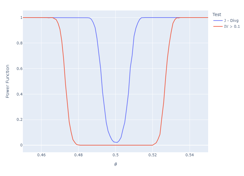
Figure 1: Comparison between power function J-Divergence test and criterion IV$>0.1$. Simulation parameters: $N=50\,300$, $n=300$, $m=50\,000$, Imbalance-Rate$\,=0,00596$, $\alpha=0.1\%$, $r=10$.

In the first simulation example, we compare the power function of our test with the power function of the criterion $\textrm{IV}>0.1$ detailed in Section 1. In this case, we measure the power function as

$$\textrm{Power-Function}=\frac{1}{M}\,\sum\limits_{i=1}^{M}\mathbf{I}[J(\hat{\mathbf{p}}_{n},\hat{\mathbf{q}}_{m})>0.1],$$ (19)

for each $\theta\in[0,1]$. The results of this comparison are shown in Figure 1. From this figure we have that, in conditions of imbalance, the superiority of the performance of our test compared to the commonly used criterion is notable. It is natural to wonder if this scenario holds at different levels of imbalance. Therefore, in Figure 2 and Figure 3 we evaluate the effect of different levels of imbalance on the performance of both methodologies. On the one hand, the performance of our test is robust to different intensities of the imbalance, see Figure 2. However, the performance of criterion IV$>0.1$ is drastically affected by high levels of imbalance, see Figure 3. Note that the green line in Figure 3 starts almost at 0.4, which represents the high Type-I error, high levels of false positives, associated with this criterion. It is worth mentioning that our test does not experience this Type-I error inflation generated by high levels of imbalance. In this sense, we say that our test is much more robust than the conventionally used criterion IV$>0.1$.

Remark 4

The hypothesis test that we propose in this work is much more robust to the presence of high levels of imbalance in the target variable.

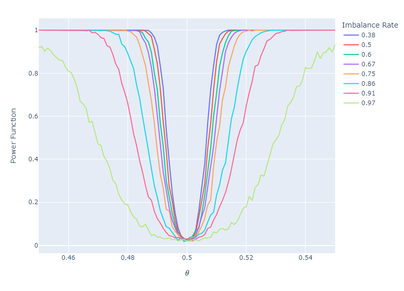
Figure 2: Power function of J-Divergence test. Simulation parameters: $r=10$, $\alpha=0.1\%$, $n=3\,000$, $m\in[100,5\,000]$.

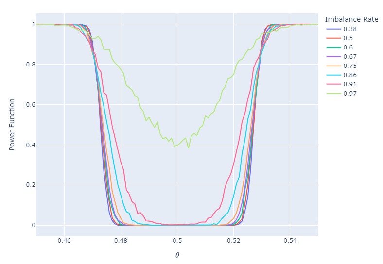
Figure 3: Power function of criterion IV$>0.1$. Simulation parameters: $r=10$, $\alpha=0.1\%$, $n=3\,000$, $m\in[100,5\,000]$.

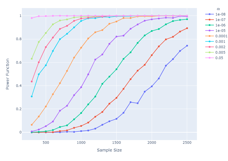
Figure 4: Power function of J-Divergence test. Simulation parameters: $n=m\in[300,2\,500]$, Imbalance-Rate$\,=0,5$, $r=10$.

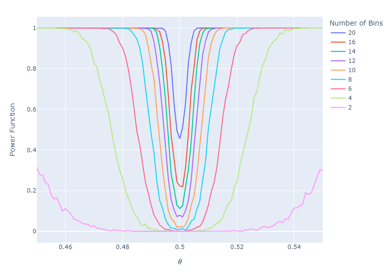
Figure 5: Power function of J-Divergence test. Simulation parameters: $n=m=3\,000$, Imbalance-Rate$\,=0,5$, $r\in[2,20]$.

It is also of primary interest to know how the performance of our test depends on the levels of statistical significance $\alpha$ and the number of bins $r$. Our test performs best for $\alpha\in[0.001\%,0.1\%]$, see Figure 4. Furthermore, our test shows robust performance, without significant Type-I error, for bin numbers $r\in[2,14]$, see Figure 5.

Remark 5

Although the optimal value for the level of statistical significance $\alpha$ and the number of bins $r$ that should be used to guarantee a good performance of the hypothesis testing proposed in this work should vary case by case, we suggest using $\alpha=0.01\%$ and $r\leq 14$.

4 Features selection in fraud detection

The data analyzed in this section are presented in detail in [16]. The data comes from Vesta Corporation real-world e-commerce transactions and contains a wide range of features from payment device type to product features. The fraud data have been organized into two bases, a trai dataset with $47,2432$ operations records and a test dataset with $118,108$ records. Both datasets are made up of 369 features and an target variable which indicates whether the operation was fraud or not. The challenge is to build classification machine learning models to detect fraud with high precision and simultaneously with low levels of false positives. To this end, the first step is to features selection based on predictive power, that is, prioritize the features that contain the most information and that will allow correct discrimination of fraudulent operations. For this first stage we have considered three alternatives: i) Do not use any characteristic selection criteria, use all available features. ii) Use the criterion IV$>0.1$. iii) Use the J-Divergence test that we have proposed in this work. The results for each selection criterion evaluated are presented in Table 2. Our test selected 42 features that the IV$>0.1$ criterion did not select. A very interesting fact is that these 42 features not considered by the second criterion contain relevant information for the detection of fraud. For example, to have a general idea, of these 42 additional features we have selected the four with the lowest p-value assigned by our test, see Table 3. These four features have a clear non-linear trend with respect to the entropy within each bin, this confirms the significant predictive power of these characteristics when identifying fraud, see Figure 6. These same patterns are repeated in the remaining variables selected by our test. Therefore, in this first stage, prior to modeling, our test satisfactorily selected features that contain relevant information for the classification problem and showed superiority with respect to second methodology.

Without Selection	Criterion IV>0.1	J-Divergence Test
369	220	262

Table 2: Features number selected for each of the three methodologies.

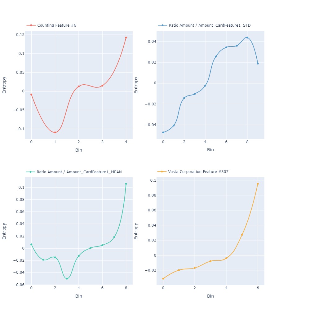
Figure 6: Shannon entropy versus bins for four features selected only by the J-Divergence test. For each graph, the horizontal axis contains the mean within each bin and the vertical axis contains the Shannon entropy measure within each bin with respect to the target variable.

Predictor	J - Estimate	Std - Error	p - value
Counting Feature #6	0.099010	0.003176	2.694e-213
Ratio Amount/Amount_CardFeature1_STD	0.085637	0.002939	1.036e-186
Ratio Amount/Amount_CardFeature1_MEAN	0.077940	0.002806	8.449e-170
Vesta Corporation Feature 307#	0.080216	0.002893	3.681e-169

Table 3: Results of the J-Divergence test for the selected variables.

In the second stage, the modeling stage, for each selected feature subset, we will use the train dataset to train a Light Gradient Boosting Machine (LightGBM) with their respective parameters optimized for each case with their respective parameters optimized for each case. The main LightGBM performance indicators on test dataset are shown in Table 4. From this table we highlight that our test has a little more than 1% in precision with respect to the second methodology IV$>0.1$, and judging by the other indicators, this increase is due to the decrease in false positives, which in this context translate into a non-negligible decrease in false fraud alerts. As mentioned above, a reduction of more than 1% in false fraud alerts generally has a considerable economic and financial impact since it avoids the blocking of many genuine paymets operations and all the inconvenience that this generates for customers. If we compare our test with the first methodology, that is, training the LightGBM without any prior feature selection criteria, we have a 3% advantage in precision with 107 fewer features. In addition to the economic impact generated by the increase in precision in fraud detection, we must consider the reduction in engineering cost, implementation cost, production and maintenance, as a consequence of the reduction of more than 100 features in the classifier. Therefore, we can argue that the appropriate use of the test proposed in this work leads to the features selection efficient prior to the modeling stage.

	Without Selection	Criterion IV>0.1	J-Divergence Test
Precision	0.85496	0.87141	0.88491
Rcall	0.74594	0.73457	0.73812
AUC	0.97098	0.97112	0.97188
F1	0.79624	0.79666	0.79734

Table 4: LightGBM performance on test dataset.

5 Implementation

In order to facilitate the usability and reproducibility of the main results of this work, we have developed the open-source python library “statistical-iv”.

6 Conclusions and future work

In this paper we propose a non-parametric hypothesis test for the IV. To our knowledge, there is no work in the literature in which a formal statistical test for this quantity has been presented. We derive efficient asymptotic formulas for the test statistic that imply that our test is consistent. Furthermore, in different scenarios, simulations show that our test easily surpasses existing empirical criteria about IV based on fixed thresholds. As imbalance is a recurring scenario in classification problems, our test works very well even for scenarios with high levels of imbalance. In a real fraud identification data set, we show the potential of our J-Divergence statistic to evaluate the predictive power of the considered features.

Although the main focus of this article is binary classification, the generalization of the J test statistic, and therefore of the IV, to the case of multinomial classification is possible. Perhaps the idea of this generalization is simple and natural, although we believe that the technical details are not so trivial and warrants future research.

Appendix: Proofs

A1. Proof of Theorem 1

Let $\phi(x,y)=(x-y)\ln\big{(}\frac{x}{y}\big{)}$, in such a way that

$$J(\hat{\mathbf{p}}_{n},\hat{\mathbf{q}}_{m})=\sum_{j\in D}\phi({\hat{p}}_{n}^{\,a_{j}},{\hat{q}}_{n}^{\,a_{j}})\quad\textrm{and}\quad J({\mathbf{p}},{\mathbf{q}})=\sum_{j\in D}\phi(p_{j},q_{j}).$$ (20)

For a fixed $j\in D$ and making use of the continuous differentiability of the function $\phi(x,y)$ along with first-order Taylor‘s theorem, see 12, we get

$$\phi({\hat{p}}_{n}^{\,a_{j}},{\hat{p}}_{n}^{\,a_{j}}) = \phi(p_{j}+\Delta_{p_{n}}^{a_{j}},\,q_{j}+\Delta_{q_{n}}^{a_{j}})$$

$$= \phi(p_{j},q_{j})+\Delta_{p_{n}}^{a_{j}}\,\partial_{x}\phi(p_{j},q_{j})+\Delta_{q_{n}}^{a_{j}}\,\partial_{y}\phi(p_{j},q_{j})+R_{j}(n,m),$$

where, for $0<\theta_{j},\eta_{j}<1$, the Lagrange’s remainder term in the following form

$$R_{j}(n,m) = \frac{1}{2}\Big{[}\big{(}\Delta_{p_{n}}^{a_{j}}\big{)}^{2}\partial_{xx}\phi\big{(}p_{j}+\theta_{j}\Delta_{p_{n}}^{a_{j}},\,q_{j}+\eta_{j}\Delta_{q_{n}}^{a_{j}}\big{)}$$

$$\qquad\qquad\qquad+2\,\Delta_{p_{n}}^{a_{j}}\Delta_{q_{n}}^{a_{j}}\,\partial_{xy}\phi\big{(}p_{j}+\theta_{j}\Delta_{p_{n}}^{a_{j}},\,q_{j}+\eta_{j}\Delta_{q_{n}}^{a_{j}}\big{)}$$

$$\qquad\qquad\qquad\qquad\qquad\qquad+\big{(}\Delta_{q_{n}}^{a_{j}}\big{)}^{2}\partial_{yy}\phi\big{(}p_{j}+\theta_{j}\Delta_{p_{n}}^{a_{j}},\,q_{j}+\eta_{j}\Delta_{q_{n}}^{a_{j}}\big{)}\Big{]}.$$

Summing over $j\in D$ in (A1. Proof of Theorem 1) we have that

$$J(\hat{\mathbf{p}}_{n},\hat{\mathbf{q}}_{m})-J(\mathbf{p},\mathbf{q})=\sum_{j\in D}\Delta_{p_{n}}^{a_{j}}\,\partial_{x}\phi(p_{j},q_{j})+\sum_{j\in D}\Delta_{q_{n}}^{a_{j}}\,\partial_{y}\phi(p_{j},q_{j})+\sum_{j\in D}R_{j}(n,m),$$ (23)

which leads to

$$|J(\hat{\mathbf{p}}_{n},\hat{\mathbf{q}}_{m})-J(\mathbf{p},\mathbf{q})|\leq A_{n}\sum_{j\in D}|\partial_{x}\phi(p_{j},q_{j})|+B_{n}\sum_{j\in D}|\partial_{y}\phi(p_{j},q_{j})|+\sum_{j\in D}|R_{j}(n,m)|.$$ (24)

In (24), notice that $\sum_{j\in D}|\partial_{x}\phi(p_{j},q_{j})|<\infty$ and $\sum_{j\in D}|\partial_{y}\phi(p_{j},q_{j})|<\infty$. In the sequel, it is easy to deduce that the third term on the right hand side of equation (24) satisfies the following inequality

$$\frac{1}{C_{n,m}}\sum_{j\in D}|R_{j}(n,m)| \leq \frac{1}{2}\bigg{[}A_{n}\,\sum_{j\in D}\big{|}\partial_{xx}\phi\big{(}p_{j}+\theta_{j}\Delta_{p_{n}}^{a_{j}},\,q_{j}+\eta_{j}\Delta_{q_{n}}^{a_{j}}\big{)}\big{|}$$

$$\qquad+2\,A_{n}\,\sum_{j\in D}\big{|}\partial_{xy}\phi\big{(}p_{j}+\theta_{j}\Delta_{p_{n}}^{a_{j}},\,q_{j}+\eta_{j}\Delta_{q_{n}}^{a_{j}}\big{)}\big{|}$$

$$\qquad\qquad\qquad\quad+B_{m}\,\sum_{j\in D}\big{|}\partial_{yy}\phi\big{(}p_{j}+\theta_{j}\Delta_{p_{n}}^{a_{j}},\,q_{j}+\eta_{j}\Delta_{q_{n}}^{a_{j}}\big{)}\big{|}\bigg{]}.$$

Based on the strong law of large numbers, we know that both $\Delta_{p_{n}}^{a_{j}}$ and $\Delta_{q_{m}}^{a_{j}}$ tends to $0$ as $n,\,m\to\infty$ almost surely, and consequently, $A_{n}$ and $B_{m}$ also tends to $0$. Based on the same argument, we have $\sum_{j\in D}\big{|}\partial_{xx}\phi\big{(}p_{j}+\theta_{j}\Delta_{p_{n}}^{a_{j}},\,q_{j}+\eta_{j}\Delta_{q_{n}}^{a_{j}}\big{)}\big{|}\to\sum_{j\in D}|\partial_{xx}\phi(p_{j},\,q_{j})|<\infty$, $\sum_{j\in D}\big{|}\partial_{xy}\phi\big{(}p_{j}+\theta_{j}\Delta_{p_{n}}^{a_{j}},\,q_{j}+\eta_{j}\Delta_{q_{n}}^{a_{j}}\big{)}\big{|}\to\sum_{j\in D}|\partial_{xy}\phi(p_{j},\,q_{j})|<\infty$, and likewise, $\sum_{j\in D}\big{|}\partial_{yy}\phi\big{(}p_{j}+\theta_{j}\Delta_{p_{n}}^{a_{j}},\,q_{j}+\eta_{j}\Delta_{q_{n}}^{a_{j}}\big{)}\big{|}\to\sum_{j\in D}|\partial_{yy}\phi(p_{j},\,q_{j})|<\infty$ as $n,\,m\to\infty$ almost surely. Therefore, from equation (A1. Proof of Theorem 1) we have to

$$\frac{1}{C_{n,m}}\sum_{j\in D}|R_{j}(n,m)|\longrightarrow 0\quad\textrm{as}\quad n,m\longrightarrow\infty,$$ (26)

almost surely. Finally, we combine equations (24) and (26), which leads us to

$$\limsup\limits_{(n,m)\rightarrow(+\infty,+\infty)}\frac{|J(\hat{\mathbf{p}}_{n},\hat{\mathbf{q}}_{m})-J(\mathbf{p},\mathbf{q})|}{C_{n,m}} \leq \sum_{j\in D}|\partial_{x}\phi(p_{j},q_{j})|+\sum_{j\in D}|\partial_{y}\phi(p_{j},q_{j})|$$

$$\leq \sum_{j\in D}|\ln(\frac{p_{j}}{q_{j}})+\frac{p_{j}-q_{j}}{p_{j}}|+\sum_{j\in D}|\ln(\frac{q_{j}}{p_{j}})+\frac{q_{j}-p_{j}}{q_{j}}|$$

$$\leq \sum_{j\in D}\Bigg{\{}\Big{|}1+\ln\Big{(}\frac{p_{j}}{q_{j}}\Big{)}\Big{|}+\Big{|}1+\ln\Big{(}\frac{q_{j}}{p_{j}}\Big{)}\Big{|}+\frac{q_{j}}{p_{j}}+\frac{p_{j}}{q_{j}}\Bigg{\}},$$

almost surely.  

A2. Proof of Theorem 2

From definition (6) we know that the $r$-tuple $n\hat{\mathbf{p}}_{n}=\big{(}n\hat{p}_{n}^{a_{j}}\big{)}_{j\in D}$ follows a Multinomial law with parameters $n$ and $\mathbf{p}$, denoted by $n\hat{\mathbf{p}}_{n}\sim\mathcal{M}(n,\mathbf{p})$. Similarly, from definition (7), $m\hat{\mathbf{q}}_{m}\sim\mathcal{M}(m,\mathbf{q})$. Therefore, applying the weak convergence of the Multinomial law, see for example Proposition 2 in [17], we have

$$\Bigg{(}\sqrt{\frac{n}{p_{j}}}\Delta_{p_{n}}^{a_{j}}\Bigg{)}_{j\in D}\overset{d}{\Longrightarrow}\quad Z_{\mathbf{p}}\sim\mathcal{N}_{r}(0,\Sigma_{\mathbf{p}})\quad\textrm{as}\quad n\longrightarrow\infty,$$ (28)

and

$$\Bigg{(}\sqrt{\frac{m}{q_{j}}}\Delta_{q_{m}}^{a_{j}}\Bigg{)}_{j\in D}\overset{d}{\Longrightarrow}\quad Z_{\mathbf{q}}\sim\mathcal{N}_{r}(0,\Sigma_{\mathbf{q}})\quad\textrm{as}\quad m\longrightarrow\infty.$$ (29)

Here $Z_{\mathbf{p}}=(Z_{p_{j}})_{j\in D}$ $\Sigma_{\mathbf{p}}$ and $Z_{\mathbf{q}}=(Z_{q_{j}})_{j\in D}$ are two independent Gaussian random vectors whit mean zero and covariance matrix $\Sigma_{\mathbf{p}}$ and $\Sigma_{\mathbf{q}}$ respectively, whose elements are

$$\big{(}\Sigma_{\mathbf{p}}\big{)}_{i,j}=(1-p_{j})\delta_{ij}-\sqrt{p_{i}p_{j}}(1-\delta_{ij}),\quad(i,j)\in D^{2},$$ (30)

and

$$\big{(}\Sigma_{\mathbf{q}}\big{)}_{i,j}=(1-q_{j})\delta_{ij}-\sqrt{q_{i}q_{j}}(1-\delta_{ij}),\quad(i,j)\in D^{2},$$ (31)

where $\delta_{ij}$ is the Kronecker delta. Using the linearity properties of the multivariate normal distribution in (28), and with the help of (30), we get

$$\sum_{j\in D}\Delta_{p_{n}}^{a_{j}}\,\partial_{x}\phi(p_{j},q_{j})\overset{d}{\Longrightarrow}\frac{1}{\sqrt{n}}\sum_{j\in D}\sqrt{p_{j}}\,\partial_{x}\phi(p_{j},q_{j})Z_{p_{j}}\quad\textrm{as}\quad n\longrightarrow\infty,$$ (32)

which the right side of equation (32) is a random variable that is normally distributed with mean zero and variance equal to

$$\frac{1}{n}\,\mathrm{V}_{1}(\mathbf{p},\mathbf{q}) = \mathbb{V}\textrm{ar}(\Bigg{(}\frac{1}{\sqrt{n}}\sum_{j\in D}\sqrt{p_{j}}\,\partial_{x}\phi(p_{j},q_{j})Z_{p_{j}}\Bigg{)}$$

$$= \frac{1}{n}\bigg{\{}\sum_{j\in D}\mathbb{V}\textrm{ar}\big{(}\sqrt{p_{j}}\,\partial_{x}\phi(p_{j},q_{j})Z_{p_{j}}\big{)}$$

$$\qquad+2\sum_{\{(i,j)\in D^{2}:\,i<j\}}\mathbb{C}\textrm{ov}\Big{(}\sqrt{p_{i}}\,\partial_{x}\phi(p_{i},q_{i})Z_{p_{i}},\sqrt{p_{j}}\,\partial_{x}\phi(p_{j},q_{j})Z_{p_{j}}\Big{)}\bigg{\}}$$

$$= \frac{1}{n}\bigg{\{}\sum_{j\in D}{p_{j}}(1-p_{j})\,\big{(}\partial_{x}\phi(p_{j},q_{j})\big{)}^{2}-2\sum_{\{(i,j)\in D^{2}:\,i<j\}}p_{i}p_{j}\,\partial_{x}\phi(p_{i},q_{i})\,\partial_{x}\phi(p_{j},q_{j})\bigg{\}}$$

$$= \frac{1}{n}\Bigg{\{}\sum_{j\in D}p_{j}(1-p_{j})\bigg{[}\bigg{(}1+\ln\frac{p_{j}}{q_{j}}\bigg{)}^{2}+\Big{(}\frac{q_{j}}{p_{j}}\Big{)}^{2}\bigg{]}$$

$$\qquad\quad\qquad\qquad\qquad-2\sum_{\{(i,j)\in D^{2}:\,i<j\}}p_{i}p_{j}\bigg{[}(1+\ln\frac{p_{i}}{q_{i}})(1+\ln\frac{p_{j}}{q_{j}})+\frac{q_{i}q_{j}}{p_{i}p_{j}}\bigg{]}\Bigg{\}}.$$

Similarly, from equations (29) and (31), we know that

$$\sum_{j\in D}\Delta_{q_{m}}^{a_{j}}\,\partial_{y}\phi(p_{j},q_{j})\overset{d}{\Longrightarrow}\frac{1}{\sqrt{m}}\sum_{j\in D}\sqrt{q_{j}}\,\partial_{y}\phi(p_{j},q_{j})Z_{q_{j}}\quad\textrm{as}\quad m\longrightarrow\infty,$$ (34)

which the right side of equation (34) is a random variable that is normally distributed with mean zero and variance equal to

$$\frac{1}{m}\,\mathrm{V}_{2}(\mathbf{p},\mathbf{q}) = \mathbb{V}\textrm{ar}(\Bigg{(}\frac{1}{\sqrt{m}}\sum_{j\in D}\sqrt{q_{j}}\,\partial_{y}\phi(p_{j},q_{j})Z_{q_{j}}\Bigg{)}$$

$$= \frac{1}{m}\Bigg{\{}\sum_{j\in D}q_{j}(1-q_{j})\bigg{[}\bigg{(}1+\ln\frac{q_{j}}{p_{j}}\bigg{)}^{2}+\Big{(}\frac{p_{j}}{q_{j}}\Big{)}^{2}\bigg{]}$$

$$\qquad\quad\qquad\qquad\qquad-2\sum_{\{(i,j)\in D^{2}:\,i<j\}}q_{i}q_{j}\bigg{[}(1+\ln\frac{q_{i}}{p_{i}})(1+\ln\frac{q_{j}}{p_{j}})+\frac{p_{i}p_{j}}{q_{i}q_{j}}\bigg{]}\Bigg{\}}.$$

Using a slight modification of the arguments in (A1. Proof of Theorem 1) and (26), it is verified the following convergence almost surely

$$\Bigg{|}\sqrt{\frac{nm}{m\mathrm{V}_{1}(\mathbf{p},\mathbf{q})+n\mathrm{V}_{2}(\mathbf{p},\mathbf{q})}}\,\sum_{j\in D}R_{j}(n,m)\Bigg{|}\longrightarrow 0\quad\textrm{as}\quad n,m\longrightarrow\infty.$$ (36)

Substituting equations (32), (34) and (36) in (23), and since $Z_{\mathbf{p}}$ and $Z_{\mathbf{q}}$ are independent random vectors, and assuming that $\frac{nm}{n+m}\longrightarrow\gamma\in(0,1)$, finally we obtain

$$\sqrt{\frac{nm}{m\mathrm{V}_{1}(\mathbf{p},\mathbf{q})+n\mathrm{V}_{2}(\mathbf{p},\mathbf{q})}}\,\Big{(}J(\hat{\mathbf{p}}_{n},\hat{\mathbf{q}}_{m})-J(\mathbf{p},\mathbf{q})\Big{)}\overset{d}{\Longrightarrow}\mathcal{N}(0,1).$$ (37)

 

Acknowledgments

This work has been partially supported by the Research Institute of the Faculty of Economics, Statistics and Social Sciences (IECOS) and the Vice-Rectorate of Research of the National University of Engineering (VRI-UNI) through the research project 25-2023-002666.

References

- 1 Howard, R. Information value theory. IEEE Transactions On Systems Science And Cybernetics. 2, 22-26 (1966)
- 2 Kullback, S. Information theory and statistics. (Courier Corporation, 1997)
- 3 Top, J. & Matthijsen, K. Information value in a decision making context. Radboud University Nijmegen. (2015)
- 4 Alsabhan, A., Singh, K., Sharma, A., Alam, S., Pandey, D., Rahman, S., Khursheed, A. & Munshi, F. Landslide susceptibility assessment in the Himalayan range based along Kasauli–Parwanoo road corridor using weight of evidence, information value, and frequency ratio. Journal Of King Saud University-Science. 34, 101759 (2022)
- 5 Batar, A. & Watanabe, T. Landslide susceptibility mapping and assessment using geospatial platforms and weights of evidence (WoE) method in the Indian himalayan region: Recent developments, gaps, and future directions. ISPRS International Journal Of Geo-Information. 10, 114 (2021)
- 6 Navas-Palencia, G. Optimal binning: mathematical programming formulation. ArXiv Preprint ArXiv:2001.08025. (2020)
- 7 Lund, B. & Raimi, S. Collapsing levels of predictor variables for logistic rgression and weight of evidence coding. MidWest SAS Users Group. 2012 pp. 16-18 (2012)
- 8 Lin, A. & Others Variable reduction in sas by using weight of evidence and information value. SAS Global Forum. 95 pp. 213 (2013)
- 9 Siddiqi, N. Credit risk scorecards: developing and implementing intelligent credit scoring. (John Wiley & SAS Business Series, 2012)
- 10 Jeffreys, H. An invariant form for the prior probability in estimation problems. Proceedings Of The Royal Society Of London. Series A. Mathematical And Physical Sciences. 186, 453-461 (1946)
- 11 Jeffreys, H. The theory of probability. (OuP Oxford, 1998)
- 12 Marsden, J. & Tromba, A. Vector calculus. (Macmillan, 2003)
- 13 Basharin, G. On a statistical estimate for the entropy of a sequence of independent random variables. Theory Of Probability & Its Applications. 4, 333-336 (1959)
- 14 Stewart, A. Jensen-Shannon Divergence: Estimation and Hypothesis Testing. (The University of North Carolina at Charlotte, 2019)
- 15 Ba, A. & Lo, G. Divergence Measures Estimation and Its Asymptotic Normality Theory in the discrete case. European Journal Of Pure And Applied Mathematics. 12, 790-820 (2019)
- 16 Addison Howard, Bernadette Bouchon-Meunier, IEEE CIS, inversion, John Lei, Lynn@Vesta, Marcus2010, Prof. Hussein Abbass. IEEE-CIS Fraud Detection. (Kaggle, 2019). https://kaggle.com/competitions/ieee-fraud-detection.
- 17 Lo, G., Kpanzou, T., Ngom, M. & Niang, A. Weak Convergence (IA): Sequences of random vectors. (Statistics, 2021)