How to train your VAE

Abstract

Variational Autoencoders (VAEs) have become a cornerstone in generative modeling and representation learning within machine learning. This paper explores a nuanced aspect of VAEs, focusing on interpreting the Kullback–Leibler (KL) Divergence, a critical component within the Evidence Lower Bound (ELBO) that governs the trade-off between reconstruction accuracy and regularization [1, 2, 3]. Meanwhile, the KL Divergence enforces alignment between latent variable distributions and a prior imposing a structure on the overall latent space but leaves individual variable distributions unconstrained. The proposed method redefines the ELBO with a mixture of Gaussians for the posterior probability, introduces a regularization term to prevent variance collapse, and employs a PatchGAN discriminator to enhance texture realism. Implementation details involve ResNetV2 architectures for both the Encoder and Decoder. The experiments demonstrate the ability to generate realistic faces, offering a promising solution for enhancing VAE-based generative models.

Index Terms—  GAN-VAE, ELBO, Posterior Collapse, Data Generation, Gaussian Mixture.

1 Introduction

Variational Autoencoders (VAEs) have emerged as a robust framework for generative modeling and representation learning in machine learning [1, 4]. Although more complex variations of VAEs have been proposed (e.g., Hierarchical VAEs [5] Wasserstein-AE [6], Beta-VAE [7] and VQ-VAEs [8]), the original VAEs continue to be of great interest due to their elegant theoretical formulation. In the pursuit of understanding and enhancing the capabilities of VAEs, this paper presents a variant of a fundamental component: the Evidence Lower Bound (ELBO). The ELBO is a critical objective function for training VAEs, encapsulating the trade-off between reconstruction accuracy and regularization. Our focus in this Work centers on a detailed analysis of the interpretation of the regularization term within the ELBO, known as the Kullback–Leibler (KL) Divergence [1, 4, 9].

The KL Divergence has a pivotal role in VAEs as it enforces alignment between the distribution of latent variables and a prior distribution, often assumed to be a Normal distribution with zero mean and unit covariance. This divergence term promotes the emergence of structured latent representations, a cornerstone of effective generative models. However, our investigation delves deeper investigate on the latent space structure. We note that the KL Divergence does not impose any constraints on the individual distributions of the latent variable associated with a datum (individual posterior); this has implications for the diversity of latent vector behaviors in VAEs. In light of these findings, our proposal reformulates the role of KL Divergence with implications for latent space modeling. Our proposal addresses a well-known challenge in VAEs: the posterior collapse phenomenon [10], which can lead to a loss of distinctiveness in generated data. Specifically, we demonstrate the successful application of our approach in generating realistic facial images while retaining crucial variations in features like hairstyles and specific facial attributes [11, 8]

The main contributions in this work are an ELBO that reduces the collapse of the posterior towards the anterior (observed as the generation of very similar, blurry images). Our ELBO can be seen as an opposite version of Beta-VAE that preferentially weights quality reconstructions and an regularization term that prevents collapse of individual posteriors to a Dirac delta. Additionally, we use a VAE-GAN type scheme that promotes realistic data. Finally, we employ a Residual type architecture for the encoder and decoder to increase the networks capabilities. The main contributions affect the training process, so our results must be compared directly with those of a standard VAE [1, 4] or Beta-VAE [7]. Qualitative comparisons of the presented results versus those reported in the classic VAE or Beta-VAE formulations show superior performance of our proposal.

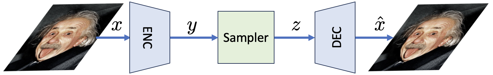
Fig. 1: General scheme of a VAE

We organize this paper as follow. We present in Section 2 a brief review of the standard VAE model. Then, in section 3, we present a mixture of Gaussian’s for defining the posterior probability $q({\bf z}|{\bf x})$ in the VAE, which leads us to redefine the ELBO, and we present practical implementation steps. Thus, we offer experimental results that support our claims in section 4. By advancing our understanding of the regularization mechanism in VAEs and its practical implications, we contribute to the ongoing pursuit of enhancing generative modeling techniques for complex data distributions. Through this Work, we hope to shed light on the interplay between regularization and diversity in latent spatial representations, contributing to the advancement of generative models in machine learning and artificial intelligence.

2 Background

Variational Autoencoder (VAE) is an extension of the traditional Autoencoder (AE) concept [1, 4]. The pivotal breakthrough of the VAE lies in its novel approach to shaping the distribution of latent variables, urging them to adhere to a simplified parametric distribution. This streamlining eases the generation of latent variables. Hence, it also facilitates the creation of complex data instances, as demonstrated by the case of faces—the example we utilize to illustrate our proposition.

The goal is to learn the generative model of ${\mathcal{D}}$ a dataset with $N\geq 1$ independent and identically distributed datapoints: ${\mathcal{D}}=\{{\bf x}^{(i)}\}_{i=1}^{N}$ with ${\bf x}^{(i)}\in\mathbb{R}^{m}$; assuming a set of latent variables, one for each datapoint: ${\mathcal{Z}}=\{{\bf z}^{(i)}\}_{i=1}^{N}$ with ${\bf z}^{(i)}\in\mathbb{R}^{d}$, and $d<m$. In this way, we have $({\bf x},{\bf z})\sim p({\bf x},{\bf z})=p({\bf x}|{\bf z})p({\bf z})$, which suggests a two-step generative model:

1. Generation of a random latent variable ${\bf z}\sim p({\bf z})$;

2. Generation of the datapoint ${\bf x}\sim p({\bf x}|{\bf z})$.

The latent variables’ distribution $p({\bf z})$ (prior) can be assumed. Then, one must estimate the conditional distribution $p({\bf x}|{\bf z})$ (likelihood). The problem arises because only the datapoints, ${\mathcal{D}}$, are observed, while the latent variables, ${\mathcal{Z}}$, remain hidden. That is, one does not know the pairs $({\bf x}^{(i)},{\bf z}^{(i)})$. To determine the ${\bf z}^{(i)}$ corresponding to ${\bf x}^{(i)}$, it is necessary to estimate the conditional distribution $p({\bf z}|{\bf x})$. Using Bayes’ rule, one can write the posterior as

$$p({\bf z}|{\bf x})=p({\bf x}|{\bf z})p({\bf z})/p({\bf x}).$$ (1)

However, calculating the evidence $p({\bf x})$ is an intractable problem [1, 4]. Therefore, instead of calculating the true posterior $p({\bf z}|{\bf x})$ one computes an approximation $q({\bf z}|{\bf x})$. A VAE is an autoencoder where: $q_{\phi}({\bf z}|{\bf x})$ is a neural network that encodes the data ${\bf x}^{(i)}$ into latent variables ${\bf z}^{(i)}$, and $p_{\theta}({\bf x}|{\bf z})$ decodes the latent variable ${\bf z}^{(i)}$ into ${\bf x}^{(i)}$; where, $\phi$ and $\theta$ are the parameters of the encoder and decoder, respectively. This stochastic generation process can be represented as:

$${\bf x}^{(i)}\overset{q_{\phi}}{\leadsto}{\bf z}^{(i)}\overset{p_{\theta}}{\mapsto}\hat{\bf x}^{(i)},$$ (2)

where $\hat{\bf x}^{(i)}$ is the generated data similar to ${\bf x}^{(i)}$. The Encoder is stochastic, meaning that if we encode $K$ times the input ${\bf x}^{(i)}$, we obtain $K$ distinct values of the latent variable: $Z^{(i)}=\{{\bf z}^{(i,k)}\}_{k=1}^{K}$. Then, the VAE’s training is performed by minimizing a cost function called the ELBO (Evidence Lower Bound):

$$\mathrm{ELBO}(\phi,\theta)= \beta\,\mathrm{KL}\bigl{(}q_{\phi}(\mathbf{z}|\mathbf{x})||p_{\lambda}(\mathbf{z})\bigr{)}$$ (3)

$$-\,\mathbb{E}_{q_{\lambda}(\mathbf{z}|\mathbf{x})}\left[\log p_{\theta}(\mathbf{x}|\mathbf{z})\right]$$ (4)

where the parameter $\beta$ weights the relative contribution of each term to the total cost. The standard VAE formulation uses $\beta=1$, meanwhile $\beta$-VAE propose to use $\beta_{1}>1$ and $\beta_{2}=1$ to improve interpretable factorised latent representations; i.e., to learn disentangled latents [11]. The second term (4) is the negative log-likelihood that enforces the generated data, $\hat{\bf x}^{(i)}$, to be likely to belong to the training dataset. The first term (3) is Kullback-Leibler divergence that enforces the approximated posterior $q_{\phi}$ to be similar to a chosen prior $p_{\lambda}$; i.e. ${\bf z}\sim p_{\lambda}({\bf z})$ and $\lambda$ are the parameters of the prior. The most common approach is to assume the prior distribution $p_{\lambda}({\bf z})$ a multivariate Gaussian with a mean of zero and an identity covariance matrix:

$$p_{\lambda}(\mathbf{z})=\mathcal{N}(0,I).$$ (5)

Since neural networks are deterministic, in order to define $q_{\phi}(\mathbf{z}|\mathbf{x})$, the stochastic behavior can implemented using the reparametrization trick:

$${\bf z}^{(i,k)}_{j}={\bf\mu}^{(i)}_{j}+\epsilon^{(k)}_{j}{\bf\sigma}^{(i)}_{j},\;\;\text{for}\;\;j=1,2,\ldots,d;$$ (6)

where $\epsilon\sim\mathcal{N}(0,I)$ and $\phi^{(i)}=({\bf\mu}^{(i)},{\bf\sigma}^{(i)})$ are the (deterministic) vectors that the network encodes the data ${\bf x}^{(i)}$ into.

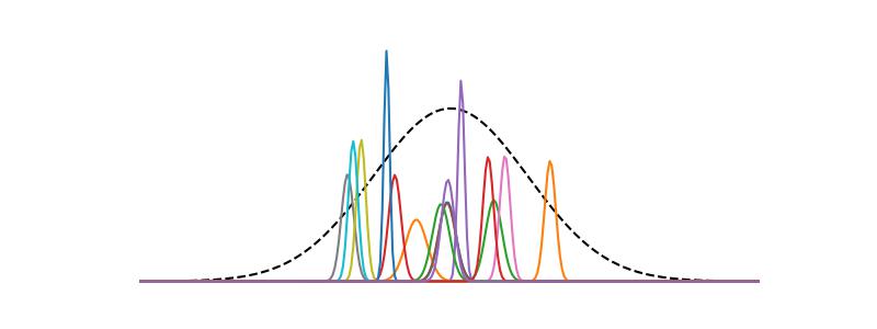
Fig. 2: Illustration of the global posterior $q_{\phi}$ as a product of individual posteriors $q_{\phi_{i}}$.

Hence, the one can factorize the posterior as [3]:

$$q_{\phi}({\bf z}|{\bf x}) =\prod_{{\bf x}^{(i)}\in\mathcal{D}}q_{\phi}({\bf z}|{\bf x}={\bf x}^{(i)})$$ (7)

$$=\prod_{{\bf x}^{(i)}\in\mathcal{D}}\mathcal{N}({\bf z};\mu^{(i)},\sigma^{(i)}).$$ (8)

This factorization takes advantage of the fact that the product of Gaussians is a Gaussian. The second row is the product of the individual posteriors (associated with each data point ${\bf x}^{i}$), and the third row makes explicit the marginals (of each latent dimension ${\bf x}_{j}$). Fig. 2 illustrates the Gaussian mixture model for the posterior. The dashed line represents the posterior $q_{\phi}$; i.e., the product of the individual Gaussian $q_{\phi}^{(i)}$ associated with each data point (in color). Note that while $q_{\phi}$ is enforced to be similar to the prior $p_{\lambda}$: a Gaussian with mean equal to zero and unitary variance. Since the KL between two univariate Gaussian is given by

$$\mathrm{KL}\bigl{(}\mathcal{N}(\mu_{1},\sigma_{1}^{2}))\|\mathcal{N}(\mu,_{2}\sigma_{2}^{2})\bigr{)}\\ =\frac{1}{2}\left[\frac{\sigma_{1}^{2}}{\sigma_{2}^{2}}+(\mu_{1}-\mu_{2})^{2}-1-\log\frac{\sigma_{1}^{2}}{\sigma_{2}^{2}}\right].$$ (9)

Thus, according with Ref. [1], the KL divergence term in the ELBO (3) takes the form:

$$\mathrm{KL}\bigl{(}q_{\phi}(\mathbf{z}|\mathbf{x})||p_{\lambda}(\mathbf{z})\bigr{)}=\sum_{j=1}^{d}\mathrm{KL}\bigl{(}\mathcal{N}(\bar{\mu}_{j},\bar{\sigma}_{j})\|\mathcal{N}(0,I)\bigr{)}\\ =\frac{1}{2}\sum_{j=1}^{d}\sum_{i:{\bf x}^{(i)}\in D}\left[(\sigma_{j}^{(i)})^{2}+(\mu^{(i)}_{j})^{2}-1-\log(\sigma_{j}^{(i)})^{2}\right];$$ (10)

where $\bar{\mu}$ and $\bar{\sigma}=\mathrm{diag}(\sigma_{j}^{2})$ are the mean vector and covariance diagonal matrix of the approximated posterior (7), respectively. The ELBO minimization is efficiently achieved by using stochastic gradient descent by using samples of the training set (mini-batches): $\mathcal{M}\subset\mathcal{D}$.

3 Method

3.1 The posterior collapse problem and over–smoothed reconstructions

VAE often suffer of the posterior collapse problem [12] (latent variable collapse or KL vanishing), such a problem occurs when $\mathrm{KL}\bigl{(}q_{\phi}(\mathbf{z}|\mathbf{x})||p_{\lambda}(\mathbf{z})\bigr{)}\rightarrow 0$. The posterior collapse to the prior results in non–identifiable latent variables: the likelihood function is independent of the latent representation producing a smoothness of the reconstructed images. To alleviate such problem there has been suggested many possible solutions, see Ref. [13] and references therein. Despite of many efforts to alleviate the posterior collapse, one can yet observe over-smoothed predictions [7, 12, 13]. It seems that only hierarchical computational expensive VAE architectures are capable of generating realistic textured data [14, 5].

To reduce the blurring, a naive strategy could consists in to reduce the parameter $\beta<1$ in (3) and passing the weight to the log-likelihood. This present another problem that we will analyze following. Note that the covariance $\bar{\sigma}$ of the posterior $q_{\phi}({\mathbf{z}}|{\mathbf{x}})$ is a diagonal (non–correlated) matrix the product in (8) can be decomposed in products of univariate Gaussians, one product for each dimension $j$. Thus, the $j$–th product results in

$$\prod_{i=1}^{N}{\cal N}(\mu_{j}^{(i)},\sigma_{j}^{(i)})=s_{j}\,{\cal N}(\bar{\mu}_{j},\bar{\sigma}_{j})$$ (11)

where

$$\frac{1}{(\bar{\sigma}_{j})^{2}} =\sum_{i=1}^{N}\frac{1}{(\sigma^{(i)}_{j})^{2}},$$ (12)

$$\bar{\mu}_{j} =(\bar{\sigma}_{j})^{2}\sum_{i}^{N}\frac{\mu^{(i)}_{j}}{(\sigma^{(i)}_{j})^{2}},$$ (13)

and $s_{j}$ is a scale factor which exact form can found in [15]. If in order to obtain reconstructions that are more faithful to the data, we weight more log–likelihood term into the ELBO then the individual posterior $q_{\phi}^{(i)}$ variance is reduced so the variations of the predictions are limited such that the VAE conducts close to a simple Autoencoder. In such case, Equations (11)–(13) make evident a problem that arise when the individual posterior $q_{\phi}^{(i)}$ approaches to a Dirac delta: $\sigma_{j}^{(i)}\approx 0$. Thus, the $j$–th entry of the posterior $q_{\phi}$ [see (7)] approaches to a Dirac Delta: $\bar{\sigma}_{j}\approx 0$. As result, the $z_{j}$ latent variable is meaningless. Therefore it is to be expected that a significantly large $\beta$ value results in more blurred reconstruction.

3.2 The posterior as a mixture of Gaussians

To introduce our proposal, first, we note that the latent variable ${\bf z}^{(i)}$, associated with the datapoint ${\bf x}^{(i)}$, is also a stochastic variable with its particular distribution, the individual posterior:

$${\bf z}^{(i)}\sim q_{\phi}({\bf z}|{\bf x}^{(i)})=q^{(i)}_{\phi}({\bf z}).$$

where $q^{(i)}_{\phi}({\bf z})=\mathcal{N}(\mu^{(i)},\sigma^{(i)})$ with $\sigma^{(i)}\succ 0$. Such individual posteriors need to be combined to define the posterior. A direct possibility is the factorization (7) but others factorization are possible. In this Work, instead of the product (7), we propose the mixture model:

$$q_{\phi}(\mathbf{z}|\mathbf{x})=\sum_{{\bf x}^{(i)}\in\mathcal{D}}\alpha_{i}\,q_{\phi}({\bf z}|{\bf x}^{(i)});$$ (14)

with $\alpha_{i}=1/N$, which implies that all data points are equally relevant. Hence, the mean of the mixture is given by:

$$\bar{\mu}=\mathbb{E}\left[q_{\phi}(\mathbf{z}|\mathbf{x})\right]=\sum_{i}\alpha_{i}\mathbb{E}\left[q_{\phi_{i}}({\mathbf{z}}|{\mathbf{x}}^{(i)})\right]=\mathbb{E}\left[{\bf\mu}^{(i)}\right],$$ (15)

and the variance of the posterior:

$$\bar{\sigma}=\mathrm{var}\left[q_{\phi}({\mathbf{z}}|{\mathbf{x}})\right]=\mathrm{var}\left[{\mathbf{z}}|{\mathbf{x}}\right].$$ (16)

Thus, we can estimate the mean and variance of the global posterior with a Stochastic Gradient strategy using data batches ${\cal D}$:

$$\bar{\mu}_{j} \approx\frac{1}{N}\sum_{i:{\mathbf{x}}_{i}\in{\cal D}}\mu^{(i)}_{j},$$ (17)

$$\bar{\sigma}^{2}_{j} \approx\frac{1}{N}\sum_{i:{\mathbf{x}}_{i}\in{\cal D}}\left({\mathbf{z}}^{(i)}_{j}-\bar{\mu}_{j}\right)^{2}.$$ (18)

This way of estimating the posterior’s mean and variance distinguishes our proposal from the standard formulation.

3.3 Loss and training strategy

In this section we present our proposal of loss. We can note that the classic $\mathrm{KL}$ formulation [1] encourages the individual means $\mu^{(i)}$’s to be zero, contributing to the so-called posterior collapse effect: the ${\mathbf{z}}^{(i)}$ are non–identifiable. Differently, in our proposal, we encourage the mean of these $\mu_{i}$’s to approach zero:

$$\mathrm{KL}_{G}\bigl{(}q_{\phi}(\mathbf{z}|\mathbf{x})\,\|\,p_{\lambda}(\mathbf{z})\bigr{)}=\mathrm{KL}\bigl{(}\mathcal{N}(\bar{\mu},I\bar{\sigma}^{2})\,\|\,\mathcal{N}(0,I)\bigr{)}\\ =\frac{1}{2}\sum_{j=1}^{d}\left[\bar{\sigma}_{j}^{2}+\bar{\mu}_{j}^{2}-1-\log\bar{\sigma}_{j}^{2}\right];$$ (19)

where $\bar{\mu}$ and $\bar{\sigma}^{2}$ are given in (17) and (18), respectively.

Furthermore, one behavior we aim to prevent is the collapse of the variances of individual posteriors $\sigma^{2}_{i}$ to zero. That eliminates the stochastic behavior of the Encoder, causing the VAE to behave like an AE. In such a scenario, the VAE would be limited to generalizing: to generate data that were not part of its training data [16].Thus, we introduce a regularization term that penalizes individual variances that become close to zero: avoiding such individual posteriors to become Dirac deltas. This regularization term is:

$$\mathrm{KL}_{I}\bigl{(}q_{\phi}(\mathbf{z}|\mathbf{x})\,\|\,p_{\lambda}(\mathbf{z})\bigr{)}\\ =\sum_{i:{\mathbf{x}}_{i}\in{\cal D}}\mathrm{KL}\bigl{(}q_{\phi}({\mathbf{z}}^{(i)}|{\mathbf{x}}^{(i)})\,\|\,\mathcal{N}(\mu^{(i)},I)\bigr{)}\\ =\sum_{i:{\mathbf{x}}_{i}\in{\cal D}}\sum_{j=1}^{d}\left[(\sigma^{(i)}_{j})^{2}-1-\log(\sigma^{(i)}_{j})^{2}\right].$$ (20)

Note that KL (20) does not penalizes the individual means.

It is well known that metrics based on pixel-to-pixel comparisons are not the most appropriate to evaluate the quality of data produced by generating models. We are willing to tolerate significant reconstruction errors as long as the reconstruction looks realistic. In the example we use, this means that we prefer to generate images where the hairstyle seems realistic, even if the positions of the curls in the reconstruction do not match the input image, rather than over-smoothing regions of the hair (as is common in a typical VAE). GAN-type models have been relatively successful in generating realistic images [17], despite suffering from the problem of modes collapse. Similar to VAE-GAN that trains the VAE based on a GAN-type scheme [18], we also use a GAN training scheme. In particular, we use a PatchGAN strategy [19, 20, 21], which instead of giving a reality measurement rating for the entire image, generates a two-dimensional array where each element evaluates a support region in the generated image or real.

Therefore the likelihood term includes two metrics, a pixel to pixel that enforce the restoration to be similar to the input data and a general evaluation grade of the image realism. For the first term we choose the L1 norm known for being robust to errors in the exact reconstruction of structures’ positions in high-frequency texture areas. This is equivalent to said that the error follows a Laplace distribution. For the second term we use a Convolutional Neural Network (Discriminator) that given the restored image $\hat{\mathbf{x}}$, of size (H,W), produces an output ${\mathbf{r}}$, of size $(h/8,w/8)$, where each entry reflects the realism degree of its support region. The discriminator is represented by the conditional ${\mathbf{r}}\sim p_{\omega}({\mathbf{r}}|{\mathbf{x}})$ where ${\mathbf{r}}\in[0,1]^{h/8\times w/8}$, and $\omega$ are the parameters of the neural network. Then the log–likelihood takes the form

$$\mathbb{E}_{q_{\lambda}(\mathbf{z}|\mathbf{x})}\left[\log p_{\theta}(\mathbf{x}|\mathbf{z})\right]=-\beta_{3}\|{\mathbf{x}}-\hat{\mathbf{x}}\|-\beta_{4}\mathrm{H}\left[{\mathbf{1}},p_{\omega}({\mathbf{r}}|\hat{\mathbf{x}})\right]$$ (21)

where $\mathrm{H}$ is the cross-entropy, $(\beta_{3},\beta_{4})$ are scale parameters, ${\mathbf{1}}$ is a vector with all its entries equal 1 which size depends on the context. Thus the regularized ELBO takes the form:

$$\mathrm{ELBO}_{reg}(\phi,\theta)=\beta_{1}\,\mathrm{KL}_{G}\bigl{(}q_{\phi}(\mathbf{z}|\mathbf{x})\,\|\,p_{\lambda}(\mathbf{z})\bigr{)}\\ +\beta_{2}\,\mathrm{KL}_{I}\bigl{(}q_{\phi}(\mathbf{z}|\mathbf{x})\,\|\,p_{\lambda}(\mathbf{z})\bigr{)}\\ -\beta_{3}\|{\mathbf{x}}-\hat{\mathbf{x}}\|-\beta_{4}\mathrm{H}\left[{\mathbf{1}},p_{\omega}({\mathbf{r}}|\hat{\mathbf{x}})\right]$$ (22)

This loss encourages the generator to produce realistic predictions $\hat{\mathbf{x}}$. In order to train the discriminator we minimize the loss

$$L(\omega)=-\beta_{4}\left(\mathrm{H}\left[{\mathbf{1}},p_{\omega}({\mathbf{r}}|{\mathbf{x}})\right]+\mathrm{H}\left[{\mathbf{0}},p_{\omega}({\mathbf{r}}|\hat{\mathbf{x}})\right]\right)$$ (23)

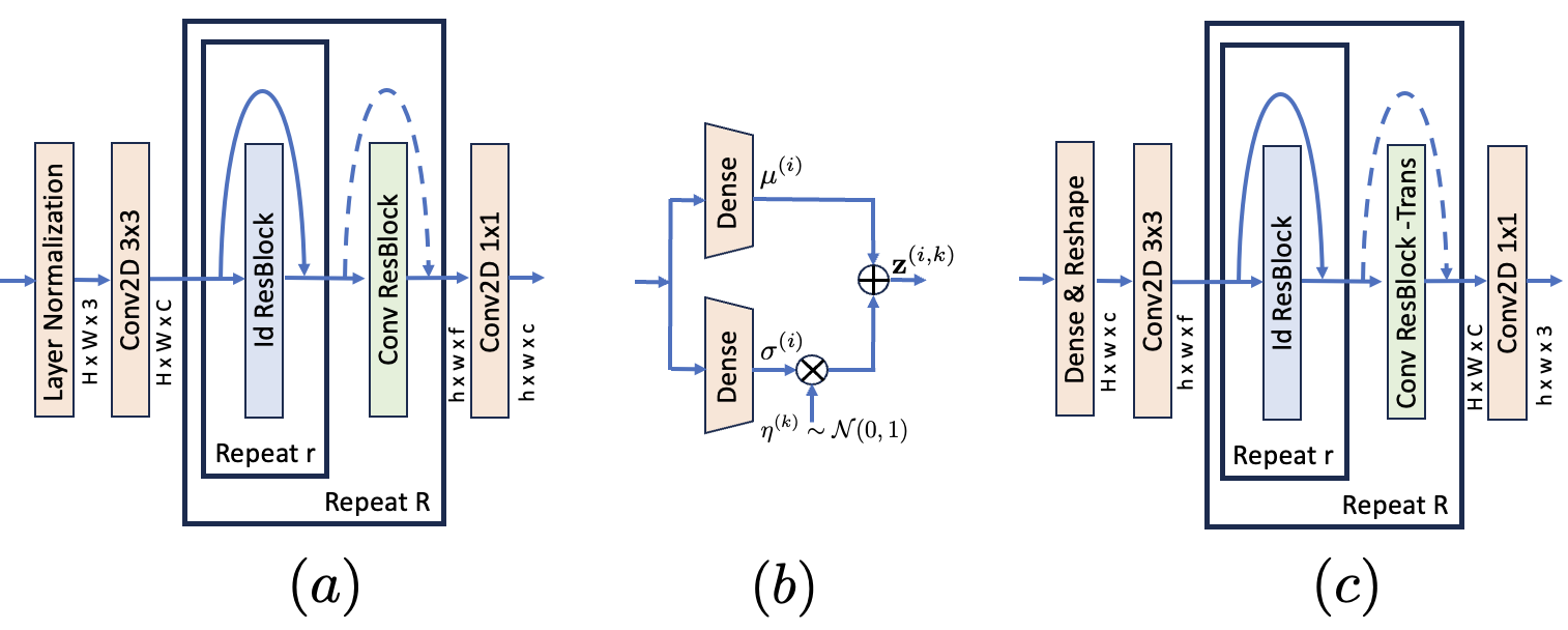
Fig. 3: Residual-VAE components. (a) Residual encoder, (b) Gaussian sampler, and (c) residual decoder.

In all the conducted experiments we kept the weight parameters: $(\beta_{1},\beta_{2},\beta_{3},\beta_{4})=(1,0.5,1000,100)$. For computational efficiency purposes, we implement the train of both, the VAE (generator) at the discriminator, using stochastic descend strategy with batch size equal $b$. Note that as the batch size $b$ becomes larger, the estimation of ELBO terms [Eqs. (19), (20) and (21)] becomes more precise. Therefore, avoiding using tiny batches is important to ensure stable convergence of the stochastic gradient. Algorithm 1 summarizes training details.

Algorithm 1 VAE-GAN Training

Given the input batch ${\mathbf{x}}$ with dimensions $(b,h,w,f)$.

1:procedure TrainStep

2:     ${\mathbf{z}}\sim q_{\phi}({\mathbf{z}}|{\mathbf{x}})$ $\triangleright$ Encode

3:     $\hat{\mathbf{x}}\sim p_{\theta}({\mathbf{x}}|{\mathbf{z}})$ $\triangleright$ Decode

4:     ${\mathbf{r}}\sim p_{\omega}({\mathbf{r}}|\hat{\mathbf{x}})$ $\triangleright$ Realism scores

5:     Take a gradient descent step on $\nabla_{\phi,\theta}ELBO_{reg}(\phi,\theta)$.

6:     Take a gradient descent step on $\nabla_{\omega}L(\omega)$.

3.4 Network architecture

Fig. 3 depicts the components in our VAE implementation. The architecture of a VAE adheres to a foundational framework, depicted in Fig. 1. Within this framework, the two fundamental components of an AE persist: the Encoder (ENC) and the Decoder (DEC). However, the hallmark that sets the VAE apart is introducing a distinctive element: the sampler. We based on ResNetV2 [22] to implement our ResidualVAE. In particular, the Identity Residual Block (Id-ResBlock), Convolutional Residual Blocks (Conv-ResBlock) and Convolutional Residual Transposed Blocks (Conv-ResBlock Trans). The ”Id-ResBlock” maintains input and output dimensions, the ”Conv-ResBlock” reduces dimensions through a stride in the convolutional layer, and ”Conv-ResBlock Trans” extends the spatial dimensions through an interpolation performed by a Transposed-Convolution layer.

4 Experiments

We show experiments designed to demonstrate that our proposal preserves the essential characteristics of VAEs while generating high-quality data. That is, the generated image is similar to the image that generated the latent variable, small variations in the latent variables introduce slight variations in the generated faces and that the interpolation of latent vectors produces realistic data with smooth transitions.

In the presented cases we use the Adam optimization method for trining the Residual-VAE and the Discriminator, we set the learning rate equal to $10^{-4}$. To demonstrate our proposal’s performance, we generate faces of $256\times 256$ pixels in RGB using the CelebA-HD database [23]. This database consists of 30,000 images that we split, after the alphanumeric ordering of files, in the first 24,000 for training and the reminder 6000 for testing.

Our first experiment demonstrates the generalization capacity of our proposal. We generate variants of a random face ${\bf x}^{\prime}$, from the test set. We obtain the variations by sampling the posterior approximation: ${\mathbf{z}}^{\prime}\sim q_{\phi}({\bf z}|{{\mathbf{x}}=\bf x}^{\prime}).$ Next, we select two entries from the latent vector: $i,j\in[1,m]$. Then, with all inputs of ${\mathbf{z}}^{\prime}$ fixed except ${\mathbf{z}}_{i}^{\prime}$ and ${\mathbf{z}}_{j}^{\prime}$, we generate images that sample the probability ($\hat{\bf x}\sim p_{\theta}({{\mathbf{x}}|{\mathbf{z}}^{\prime}})$ varying these entries for combinations of ${\mathbf{z}}_{i}^{\prime}=[-20\,\sigma^{(i)},-10\,\sigma^{(i)},0,-10\,\sigma^{(i)},-20\,\sigma^{(i)}]$ and likewise for ${\mathbf{z}}_{j}^{\prime}$. Fig. 4 shows the generated variants. As we can see, the generated faces conserve a large part of the central face. In the illustrated example, the variables ${\mathbf{z}}_{0}$ and ${\mathbf{z}}_{2}$ correspond to the horizontal and vertical axes, respectively.

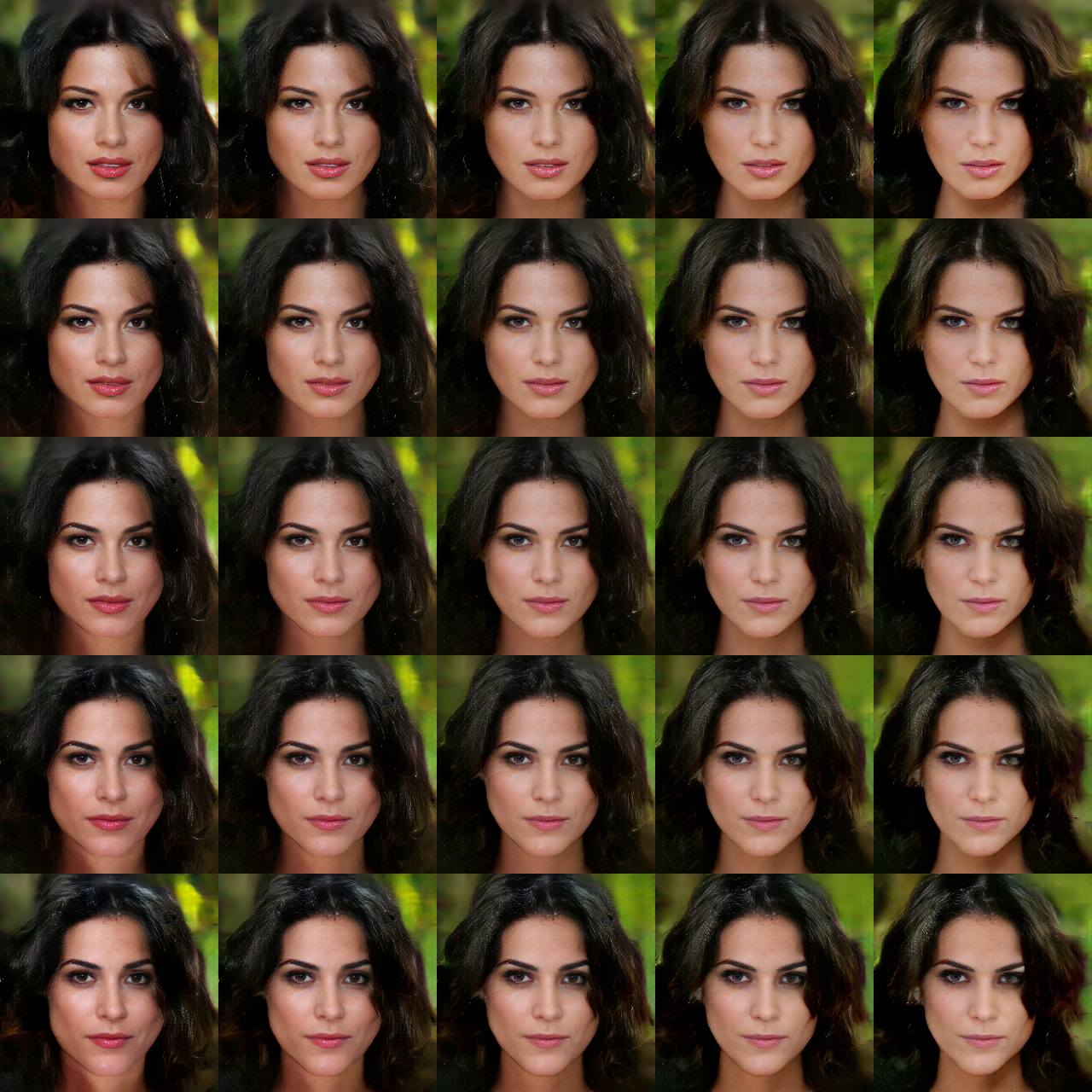
Fig. 4: VAE generated variants.

Another interesting feature of VAEs is the ability to generate transitions between two faces, where the convex combination of two latent variables corresponds to a face with characteristics smoothly transitioning from one face to another. Fig. 5 depits generated transitions. Each row corresponds to the transition between two latent variables ${\bf z}_{1}$ and ${\bf z}_{2}$, corresponding to randomly selected images in the test dataset. The columns correspond to ${\bf z}_{k}^{\prime}=(1-\alpha_{k})\,{\bf z}_{1}+\alpha_{k}\,{\bf z}_{2}$, with $\alpha_{k}=\frac{k}{(n-1)}$; for $k=0,1,\ldots,5$.

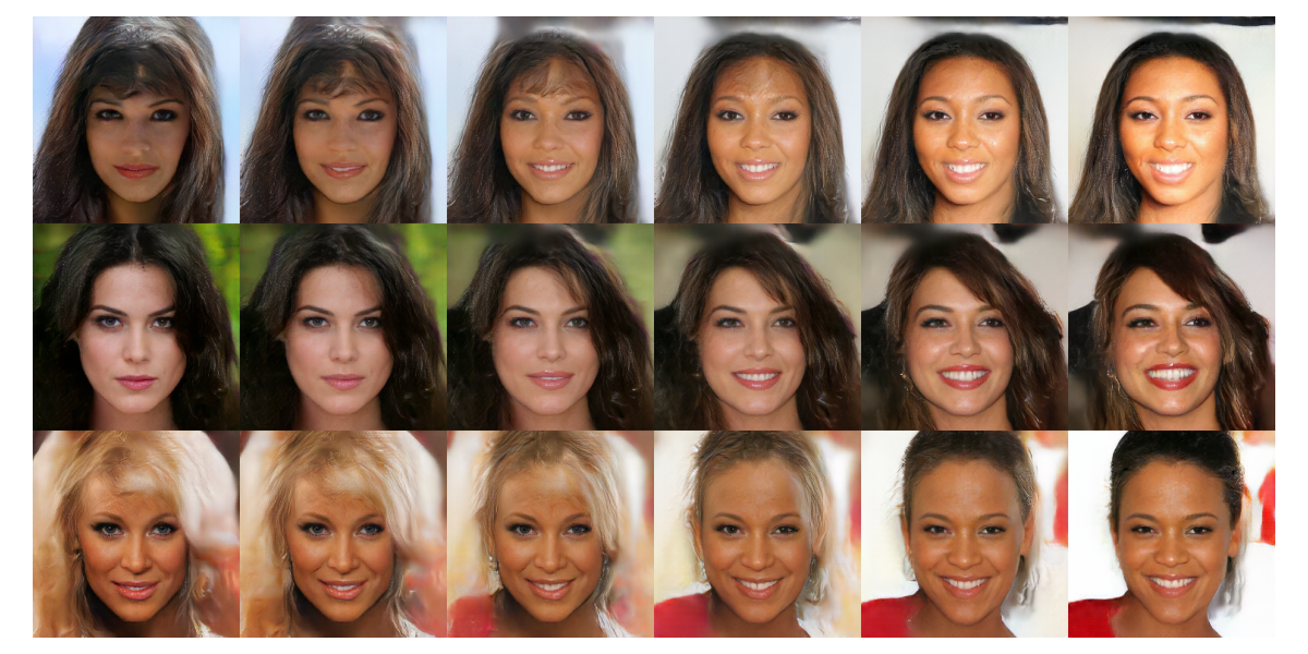
Fig. 5: VAE generated transitions: $\hat{\mathbf{x}}\sim p_{\theta}({\mathbf{x}}|{\mathbf{z}}=\alpha\,{\mathbf{z}}^{(i)}+(1-\alpha)\,{\mathbf{z}}^{(j)})$, for $\alpha\in[0,1]$; see text.

Finally, we show in Fig. 6 the joint histogram of two variables with typical estimated distributions. The histograms correspond to the latent variables ${\mathbf{z}}_{0}$ and ${\mathbf{z}}_{1}$ for 400 test data; on the right the marginal hisograms. It is notable that in our formulation 198 of 512 latent entries presented a bimodal histogram (with modes at -1 and 1). In the case of beta-VAE with beta less than 1, the collapsed histograms are monomodal and approach a Dirac delta; as Hinton noted. A more in-depth analysis of the use of these collapsed variables is beyond the scope of this article.

5 Conclusions

Our proposal substantially improves the reported results for standard VAE models while preserves the essential generative characteristics of the VAE. Although more complex variations of VAEs have been proposed (e.g., Hierarchical VAEs [5] and VQ-VAEs [8]), standard VAEs continue to be of great interest due to their elegant theoretical formulation and the promise of generating complex data from a simple distribution. Their main drawback is the posterior collapse, resulting in smoothed data. In this Work, we propose a solution to reduce these effects. Through experiments, we have demonstrated that reinterpreting the posterior as a mixture of Gaussians leads to a variant of the ELBO with a marginal computational cost. The list of our contributions in this work is as follows. First, an ELBO that reduces the collapse of the posterior towards the anterior (observed as the generation of very similar, blurry images). Our ELBO can be seen as an opposite version of Beta-VAE that preferentially weights quality reconstructions (with $\beta<1$), which is regularized to prevent individual posteriors from collapsing to a Dirac delta. Additionally, we use a VAE-PatchGAN training scheme that promotes realistic data through a discriminator that evaluates the realism of the generated data and reduces the contribution of the metric that compares pixel by pixel. Finally, we redesigned the architecture of the encoder and decoder to be of the Residual type to increase the encoding and decoding capabilities. Since the main contributions affect the training process, our results must be compared directly with those of a standard VAE or Beta-VAE. Qualitative comparisons of the results presented against those reported in the classic VAE formulations show superior performance of our proposal.

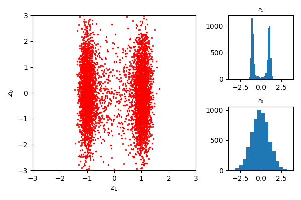
Fig. 6: Left, the join histogram of the latent variables $z_{0}$ and $z_{1}$ for the test dataset. On the right, the respective marginal histograms.

Acknowledges. Work supported in part by Conahcyt, Mexico (Grant CB-A1-43858).

References

- [1] Diederik P. Kingma and Max Welling, “Auto-encoding variational Bayes,” in 2nd International Conference on Learning Representations, ICLR, 2014.
- [2] Alexander Alemi, Ben Poole, Ian Fischer, Joshua Dillon, Rif A Saurous, and Kevin Murphy, “Fixing a broken elbo,” in International conference on machine learning. PMLR, 2018, pp. 159–168.
- [3] Diederik P Kingma, Max Welling, et al., “An introduction to variational autoencoders,” Foundations and Trends® in Machine Learning, vol. 12, no. 4, pp. 307–392, 2019.
- [4] Danilo Jimenez Rezende, Shakir Mohamed, and Daan Wierstra, “Stochastic backpropagation and approximate inference in deep generative models,” in International conference on machine learning. PMLR, 2014, pp. 1278–1286.
- [5] Jakob D Havtorn, Jes Frellsen, Søren Hauberg, and Lars Maaløe, “Hierarchical VAEs know what they don’t know,” in International Conference on Machine Learning. PMLR, 2021, pp. 4117–4128.
- [6] I Tolstikhin, O Bousquet, S Gelly, and B Schölkopf, “Wasserstein auto-encoders,” in 6th International Conference on Learning Representations (ICLR 2018). OpenReview. net, 2018.
- [7] Irina Higgins, Loic Matthey, Arka Pal, Christopher Burgess, Xavier Glorot, Matthew Botvinick, Shakir Mohamed, and Alexander Lerchner, “beta-VAE: Learning basic visual concepts with a constrained variational framework,” in International conference on learning representations, 2016.
- [8] Ali Razavi, Aaron Van den Oord, and Oriol Vinyals, “Generating diverse high-fidelity images with VQ-VAE-2,” Advances in neural information processing systems, vol. 32, 2019.
- [9] Danilo Jimenez Rezende and Shakir Mohamed, “Variational inference with normalizing flows,” in Proceedings of the 32nd International Conference on Machine Learning, 2015, pp. 1530–1538.
- [10] Junxian He, Daniel Spokoyny, Graham Neubig, and Taylor Berg-Kirkpatrick, “Lagging inference networks and posterior collapse in variational autoencoders,” arXiv preprint arXiv:1901.05534, 2019.
- [11] Irina Higgins, Loic Matthey, Arka Pal, Christopher Burgess, Xavier Glorot, Matthew Botvinick, Shakir Mohamed, and Alexander Lerchner, “-VAE: Learning basic visual concepts with a constrained variational framework,” in International Conference on Learning Representations (ICLR), 2017.
- [12] Yixin Wang, David Blei, and John P Cunningham, “Posterior collapse and latent variable non-identifiability,” Advances in Neural Information Processing Systems, vol. 34, pp. 5443–5455, 2021.
- [13] Yuhta Takida, Wei-Hsiang Liao, Chieh-Hsin Lai, Toshimitsu Uesaka, Shusuke Takahashi, and Yuki Mitsufuji, “Preventing oversmoothing in vae via generalized variance parameterization,” Neurocomputing, vol. 509, pp. 137–156, 2022.
- [14] Lars Maalø e, Marco Fraccaro, Valentin Liévin, and Ole Winther, “Biva: A very deep hierarchy of latent variables for generative modeling,” in Advances in Neural Information Processing Systems, H. Wallach, H. Larochelle, A. Beygelzimer, F. d'Alché-Buc, E. Fox, and R. Garnett, Eds. 2019, vol. 32, Curran Associates, Inc.
- [15] Paul Bromiley, “Products and convolutions of gaussian probability density functions,” Tina-Vision Memo, vol. 3, no. 4, pp. 1, 2003.
- [16] G. E. Hinton and R. R. Salakhutdinov, “Reducing the dimensionality of data with neural networks,” Science, vol. 313, no. 5786, pp. 504–507, 2006.
- [17] Antonia Creswell, Tom White, Vincent Dumoulin, Kai Arulkumaran, Biswa Sengupta, and Anil A Bharath, “Generative adversarial networks: An overview,” IEEE signal processing magazine, vol. 35, no. 1, pp. 53–65, 2018.
- [18] Anders Boesen Lindbo Larsen, Søren Kaae Sønderby, Hugo Larochelle, and Ole Winther, “Autoencoding beyond pixels using a learned similarity metric,” in International conference on machine learning. PMLR, 2016, pp. 1558–1566.
- [19] Chuan Li and Michael Wand, “Precomputed real-time texture synthesis with Markovian generative adversarial networks,” in Computer Vision–ECCV 2016: 14th European Conference, Amsterdam, The Netherlands, October 11-14, 2016, Proceedings, Part III 14. Springer, 2016, pp. 702–716.
- [20] Phillip Isola, Jun-Yan Zhu, Tinghui Zhou, and Alexei A Efros, “Image-to-image translation with conditional adversarial networks,” in Proceedings of the IEEE conference on computer vision and pattern recognition, 2017, pp. 1125–1134.
- [21] Ya-Liang Chang, Zhe Yu Liu, Kuan-Ying Lee, and Winston Hsu, “Free-form video inpainting with 3d gated convolution and temporal patchgan,” in Proceedings of the IEEE/CVF International Conference on Computer Vision (ICCV), October 2019.
- [22] Kaiming He, Xiangyu Zhang, Shaoqing Ren, and Jian Sun, “Identity mappings in deep residual networks,” in Computer Vision–ECCV 2016: 14th European Conference, Amsterdam, The Netherlands, October 11–14, 2016, Proceedings, Part IV 14. Springer, 2016, pp. 630–645.
- [23] Tero Karras, Timo Aila, Samuli Laine, and Jaakko Lehtinen, “Progressive growing of GANs for improved quality, stability, and variation,” in International Conference on Learning Representations, 2018.