Topological dualities via tensor networks

Abstract

The ground state of the toric code, that of the two-dimensional class D superconductor, and the partition sum of the two-dimensional Ising model are dual to each other. This duality is remarkable inasmuch as it connects systems commonly associated to different areas of physics – that of long range entangled topological order, (topological) band insulators, and classical statistical mechanics, respectively. Connecting fermionic and bosonic systems, the duality construction is intrinsically non-local, a complication that has been addressed in a plethora of different approaches, including dimensional reduction to one dimension, conformal field theory methods, and operator algebra. In this work, we propose a unified approach to this duality, whose main protagonist is a tensor network (TN) assuming the role of an intermediate translator. Introducing a fourth node into the net of dualities offers several advantages: the formulation is integrative in that all links of the duality are treated on an equal footing, (unlike in field theoretical approaches) it is formulated with lattice precision, a feature that becomes key in the mapping of correlation functions, and their possible numerical implementation. Finally, the passage from bosons to fermions is formulated entirely within the two-dimensional TN framework where it assumes an intuitive and technically convenient form. We illustrate the predictive potential of the formalism by exploring the fate of phase transitions, point and line defects, topological boundary modes, and other structures under the mapping between system classes. Having condensed matter readerships in mind, we introduce the construction pedagogically in a manner assuming only minimal familiarity with the concept of TNs.

I Introduction

Where they exist, dualities are powerful aides in understanding the physics of nominally different complex systems. As a case in point, consider the ground state of the toric code (TC), that of a topological superconductor (SC) in symmetry class D, and the partition sum of the classical two-dimensional Ising model (IM) — three of the main protagonists of this work. In a sense to be made precise in the following, these systems are connected by duality transformations Blackman (1982); Blackman and Poulter (1991); Blackman et al. (1998); Berezin (1969); Plechko (1985); Dotsenko and Dotsenko (1983); Merz and Chalker (2002); Castelnovo and Chamon (2008); Zhu and Zhang (2019). In the case at hand, these draw connections between bosonic and fermionic systems, ground states and partition sums, and between classical and quantum systems. They also link systems which are at the forefront of interest to different communities. For example, the toric code ground state is a paradigmatic example of a long range entangled state of matter (hence featuring intrinsic topological order) Kitaev (2003), while the topological superconductor is a free fermion system belonging to the family of topological insulators Ryu et al. (2010). All three systems display phase transitions — between an ordered phase and a topological spin liquid, a trivial and a topological superconductor and a ferro- and a paramagnet, respectively — and the duality establishes the equivalence between these. The same applies to physics at various defect structures, for example, the formation of gapless boundary modes in the superconductor related to the behavior of anyonic excitations at the boundary of the toric code.

Dualities in condensed matter physics are generically established via a toolbox of recurrent concepts. These include the mappings between $d$-dimensional quantum systems and $(d+1)$-dimensional partition sums, the taking of continuum limits mapping to (conformal) field theories and dimensional analysis, or the comparison of operator commutator algebras on different sides of the duality. For example, one way to go from the two-dimensional Ising model to the superconductor, is to first apply an anisotropic scaling deformation to map the former to the transverse magnetic field quantum Hamiltonian, then equate this bosonic system to a fermionic Majorana chain via Jordan-Wigner Onsager (1944); Kaufman (1949); Schultz et al. (1964) transformation, and finally re-discretize time to arrive at the two-dimensional lattice Hamiltonian describing a superconductor in the Majorana basis Dotsenko and Dotsenko (1983); Plechko (1985); Merz and Chalker (2002).

In this work, we consider the TC/SC/IM triplet to illustrate how tensor networks (TN) offer an efficient and intuitive alternative approach to dualityVanhove et al. (2018); Aasen et al. (2020); Lootens et al. (2023, 2022). The idea is to place a TN in the so-called matchgate category Valiant (2002); Bravyi (2009); Jahn et al. (2019); Cai and Choudhary (2006); Cai et al. (2007) as an intermediate between the three systems. There are manifold advantages to bringing in a fourth system as a translator. First, the TN comes in two incarnations, a bosonic and a fermionic one, and the passage between the two is established directly on the two-dimensional lattice by what in effect is a ‘two-dimensional Jordan-Wigner transformation’ Onsager (1944); Kaufman (1949); Schultz et al. (1964); Derby et al. (2021). In this way, we may pass from bosons to fermions avoiding dimensional detours. (The operation is conceptually similar, but somewhat more direct than previous constructions Berezin (1969); Dotsenko and Dotsenko (1983) based on the commutator algebra.)

Second, the mapping is microscopic and explicitly relates to the operator contents of all three theories. This level of detail, which is lost in continuum approaches, supports intuition and is essential in the construction of dual representations of correlation functions. We will illustrate this point on the equivalence between free Majorana correlation functions of the SC with more complex correlations between composites of spin and disorder operators Kadanoff and Ceva (1971); Fradkin (2017) (for a definition of disorder operators, see below) in the IM.

Finally, the approach keeps all three partners of the duality construction in permanent sight. In this regard, it is different from previous approaches focusing on one specific link of the duality. The principle behind this high level of versatility is that a tensor network per se (unlike a Hamiltonian) has no pre-assigned physical interpretation. More precisely, while for a TN with open indices these are identified with physical degrees of freedom, for a TN without open indices, the interpretation of individual tensors and their indices is not canonical. This ambiguity can be exploited to yield relations between seemingly unrelated physical systems. For example, the partition sum of a two-dimensional statistical mechanics model with local interactions affords interpretation in terms of a two-dimensional tensor network. Alternatively, consider the ground state of a spin system represented as a projected entangled pair state (PEPS), i.e., a tensor network on a two-dimensional graph with open indices corresponding to the Hilbert spaces of the local spins Cirac et al. (2021). The overlap of this state with itself can again be interpreted as a classical partition function. It is then natural to go one step further and establish a local correspondence between these systems by looking at the respective fine structure of their TN representations.

Supplemented with a boson-fermion mapping on the level of the TN, these ideas become even more powerful. Below, we will use such ambiguities of TN representations as a resource to discuss the full web of dualities in a comprehensive manner. In particular, we discuss a local equivalence between the partition sum of the IM and expectation values of the ground state of the toric code with string tension Castelnovo and Chamon (2008). After a boson-fermion mapping, one can furthermore equate the TN to a Grassmann integral describing the ground state of a band-insulator Hamiltonian in symmetry class D.

While the technical elements of this construction are known in the theory of matchgate tensor networks, we here present them in a comprehensive manner, aiming to introduce the key ideas to the community of condensed matter physicists. This endeavor is not just of pedagogical value: all three systems linked by the duality show rich behavior when translational symmetry is broken via the introduction of spatial phase boundaries, or defect structures. Examples include vortices, and the formation of gapless boundary modes in the superconductor, the binding of anyonic excitations at the ends of line defects in the toric code, or the physics carried by string-like ‘disorder operators’ in the Ising model. All these are subject of the duality mapping. However, the specific ways in which they transform are not always obvious. For example, the above-mentioned Majorana correlation function probes the propagation of quasi-particles injected into the superconductor ground state from one point to another. In the Ising context it becomes more complex, and now describes the correlations of a composite of a spin- and a disorder operator. The definition of the latter is non-trivial because it responds to the precise positioning of the composite operator on the Ising lattice Kadanoff and Ceva (1971); Fradkin (2017).

This and various other mappings will illustrate the application of the TN construction and are meant to introduce some powerful tricks of TN algebra to condensed matter practitioners. In a follow up publication Wille et al. (2023a) we will push this framework into less charted territory, including the presence of translationally invariance breaking disorder, the inclusion of nonlinear correlations in the TN, and that of geometrically distorted (‘holographic’) background geometries Wille et al. (2023b).

The remainder of this work is structured as follows. In Section II, we introduce the formalism of matchgate tensor networks and their representation as free fermion partition functions. Section III is the main focus of this work. It contains the derivation of the aforementioned dualities for the translation invariant case and discusses the phase transitions across the different systems. In Section IV, we extend the dualities to situations where translation invariance is broken and discuss how the duality map between different correlation functions. We summarize our work in Section V and provide an outlook to future research.

II Matchgate tensor networks

The workhorse by which the connections discussed in this work will be drawn are matchgate tensor networks (MGTN) Valiant (2002); Bravyi (2009); Jahn et al. (2019); Cai and Choudhary (2006); Cai et al. (2007). In the following, we introduce these objects in a manner assuming only a minimal level of familiarity with TNs (for introductory reviews, see Refs. Orús (2014); Eisert et al. (2010); Bridgeman and Chubb (2017); Orús (2019); Cirac et al. (2021)).

II.1 Bosonic matchgate tensors

Matchgate tensors.

A bosonic normalized, even matchgate (MG) tensor $T$ tensor carries $n$ indices $i_{j}=0,1$ of bond dimension two. As such it is described by complex coefficients $T_{i_{1}i_{2}\ldots i_{n}}$ such as $T_{0100\dots}$. To make it a matchgate tensor, we need to add further structures. Concretely, a matchgate tensor satisfies the following rules.

• (Normalization) $T_{0\ldots 0}=1$.

• (Evenness) If $i_{1}+\ldots+i_{n}$ is odd, $T_{i_{1}\ldots i_{n}}=0$.

• (Gaussianity) The ${n\choose 2}=n(n-1)/2$ so-called second moments $T_{i_{1}\ldots i_{n}}$ with $i_{1}+\ldots+i_{n}=2$ are independent. We collect them in an anti-symmetric $n\times n$- matrix $A^{T}=-A$, where $A_{12}=T_{110\ldots 0}$, $A_{13}=T_{1010\ldots 0}$, etc.

By definition, higher moments of $T$, i.e., entries with $i_{1}+\ldots+i_{n}>2$, are given by Pfaffians of submatrices of $A$. These submatrices are obtained by deleting all rows and columns $k$ for which $i_{k}=0$. For example, for a tensor with six indices the tensor entry $T_{111100}$ is given by $\mathrm{Pf}A|_{56}$, where $A_{56}$ is the sub-matrix of $A$ obtained by deleting the rows and columns 5 and 6. For a tensor with four indices, the matrix

$$A=\begin{pmatrix}0&a_{12}&a_{13}&a_{14}\\ -a_{12}&0&a_{23}&a_{24}\\ -a_{13}&-a_{23}&0&a_{34}\\ -a_{14}&-a_{24}&-a_{34}&0\end{pmatrix}$$ (1)

uniquely specifies all tensor entries. For example, $T_{1100}=a_{12}$, $T_{1010}=a_{13}$, etc. The only non-trivial higher moment is given by $T_{1111}=\mathrm{Pf}(A)$.

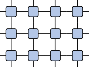
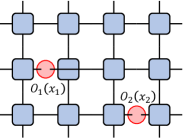
Figure 1: Translation invariant two-dimensional square lattice tensor network of tensors $T$ (left) and tensor network with incisions (right) that allow to calculate arbitrary $n$-point correlation functions of local observables, here $\langle O_{1}(x_{1})O_{2}(x_{2})\rangle$.

Matchgate tensor networks.

We now consider two-dimensional square-lattice networks of matchgate tensors as shown in Fig. 1. First consider the fully contracted TN, without open physical indices. As such, it is just a number (much as a partition sum is just a number), and not very interesting in its own right. To obtain information about, e.g., correlations, we may cut bonds to define open indices. For example we can calculate the correlation function $\langle O_{1}(x_{1})O_{2}(x_{2})\rangle$ of local observables $O_{1,2}$ by incisions at two points $x_{1},x_{2}$ as shown in Fig. 1.

II.2 Mapping to Gaussian fermionic tensor networks

Bosonic matchgate tensor networks afford a reinterpretation as Gaussian fermionic tensor networks Bravyi (2009). To establish this connection, we first review the concept of (Gaussian) fermionic tensor networks as such.

Fermionic tensor networks have been introduced to represent many-body states of fermions Barthel et al. (2009); Corboz et al. (2010); Pižorn and Verstraete (2010); Kraus et al. (2010); Gu et al. (2010); Bultinck et al. (2017). In one Gu et al. (2010) of several optional representations a fermionic tensor $T_{\text{f}}$ with $n$ indices of bond dimension two contains $n$ Grassmann variables $\theta_{j}$

$$T_{\text{f}}=T_{i_{1}\ldots i_{n}}\theta_{1}^{i_{1}}\ldots\theta_{n}^{i_{n}}\;$$ (2)

(see also Refs. Wille et al. (2017)). We may identify these with fermion states, $\theta_{i}\mapsto c_{i}^{\dagger}|0\rangle$, which are either occupied or unoccupied depending on the value $i_{j}=0,1$. Throughout, we work with tensors of even fermion parity, $T_{i_{1}\ldots i_{n}}=0$ if $i_{1}+\ldots+i_{n}\mod 2=1$.

For two tensors $A=A_{i_{1}i_{2}\ldots}\theta_{A1}^{i_{1}}\theta_{A2}^{i_{2}}\ldots$ and $B=B_{k_{1}k_{2}\ldots}\theta_{B1}^{k_{1}}\theta_{B2}^{k_{2}}\ldots$, the formal product $AB$ represents a superposition of states with up to $2n$ fermions via the above identification. We define a contraction of indices $Aj$ and $Bl$ by projection onto all states with equal occupation of $Aj$ and $Bl$ fermions. The basic mathematical identity realizing this contraction reads

$$\int\mathrm{d}\theta_{Aj}\mathrm{d}\theta_{Bl}\,e^{\theta_{Bl}\theta_{Aj}}\theta_{Bl}^{k_{l}}\theta_{Aj}^{i_{j}}=\delta^{k_{l}i_{j}}.$$

This contraction carries an orientation as contracting $Aj$ with $Bl$ differs from contracting $Bl$ with $Aj$. Before using the identity above the Grassmann variables $\theta_{Aj}$ and $\theta_{Bl}$ first need to be permuted through the remaining variables such that they come to stand upfront in the indicated order. The contraction of generic indices thus comes with a sign factor.

The generalization to multiple tensors $T^{\alpha}$, $\alpha=1,\dots,N$ with $n_{\alpha}$ fermions each is straightforward: introduce the vector $\underline{\theta}=(\theta_{11},\ldots,\theta_{1n_{1}},\ldots,\theta_{N1},\ldots\theta_{Nn_{N}})$ containing all fermionic modes, and an anti-symmetric matrix $C$ indicating the pattern of (oriented) contractions as $C_{\alpha i,\beta j}=1$, if the $i$-th mode of tensor $T^{\alpha}$ is contracted with the $j$-th mode of tensor $T^{\beta}$. The contraction of the network is then implemented by the integral

$$\text{TN}_{(C,T)}=\int(\mathrm{d}\theta)_{C}\,e^{\frac{1}{2}\underline{\theta}^{T}C\underline{\theta}}\;T^{1}\ldots T^{N}\;,$$ (3)

where $(\mathrm{d}\theta)_{C}$ is a shorthand notation for the product of all ordered pairs $\mathrm{d}\theta_{\alpha i}\mathrm{d}\theta_{\beta j}$ with $C_{\alpha i,\beta j}=1$.

Gaussian fermionic tensor networks. A tensor $T$ with $n$ indices is a fermionic Gaussian (fG) tensor if there exists a real anti-symmetric $n\times n$-matrix $A=-A^{T}$ such that

$$T_{\text{fG}}=e^{\frac{1}{2}\underline{\theta}^{T}A\underline{\theta}}\;,\quad\underline{\theta}^{T}=(\theta_{1},\ldots,\theta_{n})\;.$$ (4)

The tensor product of two fG tensors $T_{1}$, $T_{2}$ is again a Gaussian tensor given by

$$T_{\text{1}}T_{\text{2}}=e^{\frac{1}{2}\underline{\theta}^{T}(A_{1}\oplus A_{2})\underline{\theta}}\;,\quad\underline{\theta}=(\underline{\theta}_{1},\underline{\theta}_{2})\;.$$ (5)

Including the contractions in Eq. (3), we write the contracted fermionic Gaussian tensor network as

$$\text{TN}_{(C,A)}=\int(\mathrm{d}\theta)_{C}\,e^{\frac{1}{2}\underline{\theta}^{T}(A+C)\underline{\theta}}\;,$$ (6)

where $A=\oplus_{i}A_{i}$ is the direct sum of all individual characteristic functions of the tensors $T_{i}$.

Note that a real fermionic Gaussian tensor network can be interpreted as the partition sum $Z=\int\mathrm{d}\underline{\theta}e^{-S}$ with the weight

$$S=\frac{\mathrm{i}}{2}\theta^{T}H\theta\;,\quad H=\mathrm{i}(A+C)\;,$$ (7)

where $H=H^{\dagger}$ and $H=-H^{T}$. Within the framework of the tenfold symmetry classification of free fermions systems, this is a Hamiltonian in symmetry class D.

Matchgates as Gaussian fermionic tensors. Eq. (4) implies the advertised connection between fermionic Gaussian and bosonic matchgate tensors: Given a bosonic $T_{\text{MG}}$ with second moments $A$, we define

$$T_{\text{fG}}=(T_{\text{MG}})_{i_{1}\ldots i_{n}}\theta_{1}^{i_{1}}\ldots\theta_{n}^{i_{n}}=e^{\frac{1}{2}\underline{\theta}^{T}A\underline{\theta}}\;.$$ (8)

The indicated ordering of Grassmann variables is an essential element of the map $T_{\textrm{MG}}\mapsto T_{\textrm{fG}}$.

The assignment Eq. (8) remains formal unless we have settled the following consistency issue: For a (partially) contracted matchgate tensor network one may either first turn to a fermionic representation of the individual tensors and then contract according to Eq. (6), or contract first and then fermionize the result. We must make sure that the ordering of operations does not matter. Referring for a detailed discussion to App. A, we need to choose an orientation of contracted fermionic bonds and a matching ordering of contracted bosonic indices. It turns out that for any tensor network patch with disk topology an assignment consistent according to the above criterion is possible. More precisely, the order of operations is inessential up to a known factor depending on the parity of the number of uncontracted boundary fermion modes which does not have an affect of bulk properties of the tensor network. We caution that more care is required in situations with more complex boundaries. These arise, for example, in the calculation of $n$-point correlation functions, corresponding to $n$ additional punctures of the patch (see Section IV.1 for the discussion of such a setting.) We finally note that in our approach the above two-dimensional construction is key to the duality between bosonic and fermionic systems; it here assumes a role otherwise taken by the one-dimensional Jordan-Wigner transformations in approaches operating by dimensional reduction.

II.3 Factorizing tensors

As a final prerequisite for formulating our duality, we need a few added structures: A $\mathbb{Z_{2}}$-tensor $T_{\mathbb{Z_{2}}}$ has bond dimension $2$ and is defined by the parity condition $(T_{\mathbb{Z}_{2}})_{abcd}=\delta_{a+b+c+d\,\textrm{mod}2,0}$. It is straightforward to verify that the $\mathbb{Z}_{2}$ tensor satisfies the matchgate condition. In a next step, we generalize the tensor to the presence of additional weights, $W_{i}$ attached to the links, cf. Fig. 3(a), where the $\mathbb{Z}_{2}$ tensors are circles, and the weights boxes. The latter are defined as $W_{i}=\text{diag}(1,w_{i})$, i.e., diagonal matrices. This generalization, too, satisfies the matchgate condition, with the defining matrix given by $A_{ij}=w_{i}w_{j}$. Conversely, matchgate tensors whose Gaussian weights can be written in this way are called factorizing.

While simple parameter counting shows that not every matchgate tensor can be factorizing , they will be sufficient for our purposes. Specifically, the uniform matchgate tensor defined by a single parameter $a$ is the simplest example of a factorizing matchgate and its weights are $W_{i}=W:=\textrm{diag}(1,\sqrt{a})$.

III Dualities from matchgate tensor networks

In this section, we will employ the bosonic and the fermionic TNs introduced above as tools to establish the duality between the three systems mentioned in the introduction, the ground state of the toric code, that of the two-dimensional class D superconductor, and the partition sum of the classical Ising model. Our focus here, will be on the physics of the translationally invariant bulk systems, and their respective phase transitions. The fully contracted bosonic TN then corresponds to the partition function of the IM and likewise, the norm of a toric code ground state with string-tension, while the fully contracted fermionic TN evaluates to the Pfaffian of a free-fermion Hamiltonian in symmetry class D. However, the identifications between these three systems can be made locally on patches of the respective tensor networks. In Section IV, we take advantage of this fact and extend the mappings to correlation functions and defect structures, starting what could be called a dictionary between the different models dual to each other.

Previous work

To put our discussion into a larger context, we begin this section with a review of previous studies of specific links of the duality web.

IM $\to$ SC.

Previous mappings of the classical Ising partition sum onto the SC ground state can roughly be divided into two categories. The first starts from a representation of the Ising partition function on a $L\times L$ square lattice as a product of $L$ transfer matrices, where each $2^{L}\times 2^{L}$-matrix represents one column of the Ising model. This formulation stands in the tradition of Onsager’s solution Onsager (1944), which was subsequently simplified by Kaufman Kaufman (1949), and later by Schultz, Mattis and Lieb Schultz et al. (1964). One dimensional Jordan-Wigner transformations are then performed on the $2^{L}$-dimensional representation spaces of the transfer matrix to arrive at an interpretation in terms of (Majorana) fermion ground states Gogolin et al. (2004).

A more isotropic approach has been developed by Kac and Ward Kac and Ward (1952) who have expressed the partition function in terms of the determinant of a $4L\times 4L$ matrix by purely combinatorial considerations. This was followed by Hurst and Green Hurst and Green (2004) who suggested a formulation using the Pfaffian method (later refined by Blackmann and others Blackman (1982); Blackman and Poulter (1991); Blackman et al. (1998); Plechko (1985)). They noted, that the matrix for which one computes the Pfaffian is essentially that of a tight-binding Hamiltonian and as such can be interpreted as a free fermion system in 2D. This approach was recast in the language of Grassmann variables by Berezin Berezin (1969) and a formulation close in spirit to the one discussed below has been presented by Dotsenko and Dotsenko in Ref. Dotsenko and Dotsenko (1983).

Finally, in more recent works Cho and Fisher (1997); Read and Ludwig (2000); Gruzberg et al. (2001); Merz and Chalker (2002), the connection between the IM and non-interacting fermions was discussed in the context of network models and a connection between network models and Gaussian fermionic tensor networks was noted in Ref. Jian et al. (2022).

TC $\to$ IM.

To the best of our knowledge, the duality of the IM partition sum and a TC with string tension was first explored by Castelnovo and Chamon Castelnovo and Chamon (2008) and later generalized in Ref. Zhu and Zhang (2019).

SC $\to$ TC.

We are not aware of previous mappings of the TC ground state to that of the SC, although they are of course implied by the sequence TC $\to$ IM $\to$ SC.

This work

Our starting point in this work is a translationally invariant matchgate tensor network on a square lattice as shown in Fig. 1. Its tensors are characterized by a single real parameter $a$ via $a_{ij}=a$ (see Eq. (1)). All three target systems, IM, TC, SC, too, are controlled by single parameters, to be interpreted as dimensionless coupling strength, the string tension and the band-inversion parameter, respectively. Our discussion will show how these are to be related to the TN parameter $a$. In each case, the parameter $a$ drives a phase transition — the Ising ferro-/paramagnetic transition, the transition between a topological spin liquid and an ordered state, and the transition between a topological and a trivial superconductor (cf. Fig. 2). While the latter two are between states of different topological order, the first is a conventional symmetry breaking transition. The equivalence between these drastically different types of phase transitions is not a contradiction since the duality transform establishing it is intrinsically non-local.

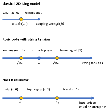
Figure 2: Phase transitions in a homogeneous single parameter matchgate tensor network interpreted in terms of three different physical systems. The control parameters $a_{\pm}=\sqrt{2}\pm 1$. In the lower panel, $c$ denotes the topological (Chern) index.

III.1 Classical two-dimensional Ising model

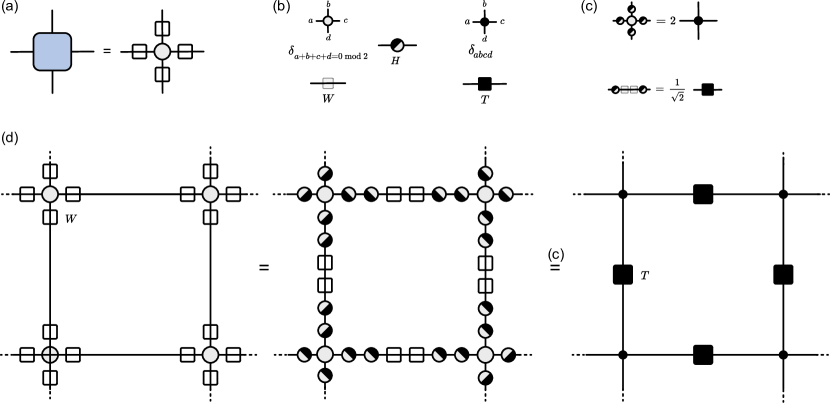
Figure 3: (a) A factorizing matchgate tensor decomposes into a $\mathbb{Z}_{2}$ tensor and weight matrices. (b) Graphical notation for the $\mathbb{Z}_{2}$ tensor (white circle), the weight matrices $W$(unfilled square), the Hadamard matrix $H$ (half filled circle, the Kronecker $\delta$-tensor (black circle) and the IM transfer matrix (black square). (c) Tensor identities used to transform a MGTN to the partition sum of the IM. (d) Transforming a weighted $\mathbb{Z}_{2}$-tensor network (left) to the Ising partition function tensor network (right) via a gauge transformation.

We start by discussing the interpretation of a factorizing matchgate tensor network as the partition function of the classical two-dimensional Ising model. This connection follows from the option to realize the even parity constraint obeyed by matchgate tensors in terms of superpositions of weighted closed loops reminiscent of the high-temperature expansion of the Ising partition function. Here, we derive the equivalence exploiting the invariance of a tensor network under basis changes in the virtual space.

We start from a representation of our tensors in terms of $\mathbb{Z}_{2}$-tensors with weights $W$ (see left panel in Fig. 3(d)). Next, we insert products of Hadamard matrices

$$H=\frac{1}{\sqrt{2}}\left(\begin{array}[]{cc}1&1\cr 1&-1\end{array}\right)$$ (9)

at all legs as shown in the center of Fig. 3(d). With $H=H^{\dagger}=H^{-1}$ this is conceptually a gauge transformation. It is straightforward to verify using the relations shown in Fig. 3(c) that this operation induces a transformation ($\mathbb{Z}_{2}$-tensors) $\mapsto$ ($2\times\delta$-tensors) where the $\delta$-tensor is defined by the condition

$$\delta_{abcd}=\delta_{ab}\delta_{bc}\delta_{cd}$$ (10)

(see Fig. 3(b)). The transformed weight matrices assume the form

$$T:=\sqrt{2}HW^{2}H=\frac{1}{\sqrt{2}}\left(\begin{array}[]{cc}1+a&1-a\cr 1-a&1+a\end{array}\right).$$ (11)

Assuming $a<1$, we define $\beta>0$ by

$$J\beta=\operatorname{artanh}(a)$$ (12)

and $h_{00}=h_{11}=-J$ and $h_{01}=h_{10}=J$, in order to identify $T$ with the transfer matrix of the Ising model,

$$T=\begin{pmatrix}e^{-\beta h_{00}}&e^{-\beta h_{01}}\\ e^{-\beta h_{10}}&e^{-\beta h_{11}}\end{pmatrix}.$$ (13)

The identification of the two non-vanishing configurations (all links 1 or all links 0) admitted by the central $\delta$-tensor identified with an Ising spin then implies an equivalence of the tensor network with the classical partition sum of the Ising model.

The two-dimensional Ising model has its magnetic phase transition at $2J_{c}\beta_{c}=\ln(1+\sqrt{2})$, or $a_{-}:=\sqrt{2}-1$, consistent with the above assumption $a<1$ (see the upper panel of Fig. 2). In the opposite case, $a>1$, we apply a global rescaling of each bond by $a^{-1}$ to send the weight matrices to $W=\text{diag}(a^{-1/2},1)$. We then use the invariance of the $\mathbb{Z}_{2}$-tensors under a simultaneous spin flip $\sigma_{x}^{\otimes 4}$ to transform to weights $W^{\prime}=\sigma_{x}W\sigma_{x}=\text{diag}(1,a^{-1/2})$, i.e., we effectively map $a\mapsto a^{-1}$. In this case, the phase transition is at $a_{+}=a_{-}^{-1}=\sqrt{2}+1$. For $a<0$, a global rescaling $a\mapsto-a$ shows the equivalence to the $a>0$ parameter domain. We conclude that our one-parameter family of tensor networks supports the four parameter intervals, $a<-1,-1\leq a<0,0\leq a<1$ and $1\leq a$ which are individually equivalent to the Ising models with critical points at $a=\pm a_{\pm}$, respectively.

III.2 Toric code with string tension

We now turn to our second interpretation of a factorizing matchgate tensor network and show how it is related to the wavefuntion of the toric code with string tension. (For a direct link TC $\leftrightarrow$ IM, not using a TN intermediate, we refer to Refs. Castelnovo and Chamon (2008); Isakov et al. (2011).)

The toric code Hamiltonian (without string tension) Kitaev (2003) is given by

$$H_{\text{TC}}=-\sum_{v\in\text{vertices}}\;\prod_{i\in v}\sigma_{z}^{(i)}-\sum_{p\in\text{plaquette}}\;\prod_{i\in p}\sigma_{x}^{(i)},$$ (14)

and its ground state vector $\ket{\Psi_{0}}$ is an equal weight superposition of closed loops of $\ket{1}$-vectors in a background of $\ket{0}$-vectors on the underlying square lattice. The toric code is a most paradigmatic example of a $\mathbb{Z}_{2}$ spin liquid and at the same time the most studied code for topological quantum error correction Dennis et al. (2002).

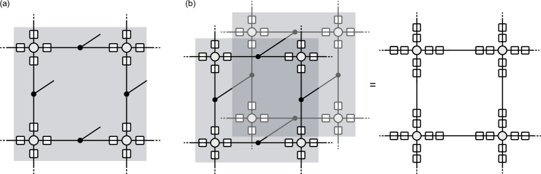
Figure 4: Toric code with string tension. (a) Ground state vector $\ket{\Psi(t)}$ represented as a PEPS, physical indices coming out of the plane. (b) The overlap $\braket{\Psi(t)}{\Psi(t)}$ given by contracting the physical indices of the PEPS and its conjugate, represented by the mirror image.

This state affords a representation in terms of a simple $\mathbb{Z}_{2}$ factorizing matchgate tensor network Verstraete et al. (2006); Gu et al. (2009); Schuch et al. (2010): First consider a configuration with uniform $a=1$. This is equivalent to a network of $\mathbb{Z}_{2}$-tensors with trivial weights. The job of the former is to admit configurations with $0,2$ or $4$ $\ket{1}$ state vectors at each vertex, with equal weight. Summation over all of these is equivalent to a uniform weight closed loop superposition. To turn this sum into a quantum state, we add $3$-leg $\delta$-tensors at each vertex (see Fig. 4(a)). The tensor product of uncompensated physical indices then defines the quantum ground state.

In the toric code context, the loop sum may be turned into a weighted one by adding string tension which penalizes or favors loops of increasing length. To mimic this effect, we generalize the tensor network to the presence of weights $W=\text{diag}(1,\sqrt{t})$ per half-edge defining the state vector $\ket{\Psi(t)}$. Each $\ket{1}$ link now comes with a factor $t$, compared to $1$ for $\ket{0}$ links. In the extreme case of $t=0$, we obtain a trivial ferromagnet polarized in the $\ket{0}$-state, in the opposite limit $t\to\infty$ the system is polarized in the $\ket{1}$-state.

The exact parent Hamiltonian of this state is given by $H=H_{\text{TC}}+H_{\text{ST}}$ with

$$H_{\text{ST}}=\sum_{v\in\text{vertices}}\prod_{i\in v}e^{-\ln t\,\sigma_{z}^{(i)}}\;.$$ (15)

In the vicinity of $t\simeq 1$, the string tension term reduces to a conventional on-site magnetic field Hamiltonian $H_{\text{ST}}\simeq-2\ln t\sum_{i}\sigma_{z}^{(i)}$.

The critical values of the string tensions inducing a transition between the topological spin liquid state and ferromagnetic states with $\ket{1}$ or $\ket{0}$ polarization $t^{2}=a_{\pm}=\sqrt{2}\pm 1$ can be derived via the mapping to the classical Ising model. The idea is to detect a phase transition via the emergence of power law correlations in correlation functions $C_{t,\alpha\beta}=\braket{\Psi(t)}{O_{\alpha}O_{\beta}}{\Psi(t)}$, where $O_{\alpha}$ and $O_{\beta}$ are local operators of the spin variables at sites $\alpha$ and $\beta$. The operator insertion between two states means that we are now dealing with a two layered tensor network where all physical indices except for those at $\alpha,\beta$ of that representing $\ket{\Psi(t)}$ are contracted with that representing $\bra{\Psi(t)}$ (see Fig. 4(b)). The consequences of this almost complete contraction are detailed in Appendix C and can be summarized as follows: the contraction of the $\delta$-tensors sitting on the bonds effectively causes a collapse of double bonds (representing bra- and ket-state) to a single one. On this effective bond, we have the square of two amplitude weights, i.e., the effective weight $W^{2}=\text{diag}(1,t)$. This is equivalent to a matchgate tensor with uniform $A$ matrices for which $a_{ij}=t^{2}$ and implies criticality at $t^{2}_{\pm}=a_{\pm}$, in agreement with the values reported in Refs. Castelnovo and Chamon (2008); Isakov et al. (2011); Zhu and Zhang (2019) (see middle panel of Fig. 2).

III.3 Class D superconductor

Our third construction establishes a connection to the topological SC. For the convenience of readers not well-versed in the physics of topological superconductivity, a brief review is included in Appendix B. The punchlines of this discussion are that (a) the free fermion Hamiltonian of a class D superconductor affords a representation in terms of a Majorana bi-linear form

$$\hat{H}:=i\Theta^{T}H\Theta,$$ (16)

where $H$ is the first quantized Hamilton matrix, and the components of $\Theta$ Majorana operators, to be identified as real and imaginary parts of complex fermion creation and annihilation operators. (b) In a translationally invariant system, the eigenstates of $H$ define Bloch bands, labeled $n$, which individually carry Chern numbers $c_{n}$. (c) Transitions between states of different topology change these numbers (at a conserved total number $\sum_{n}c_{n}=0$) and are signaled by a change of the $\mathbb{Z}$-valued topological index $c=\sum_{n=1}^{N}c_{n}$ over Chern numbers carried by individual Bloch bands, $n=1,\dots,N$, with band energies below the superconductor band gap at $\epsilon=0$. (d) Such changes of integer invariants require touching of the bands $n$ and $n+1$ involved in the change of Chern numbers. In the vicinity of these hotspots in the Brillouin zone, the local Hamiltonian may be approximated by a two-dimensional Dirac Hamiltonian

$$H^{(2)}=\kappa(q_{1}\sigma_{1}+q_{2}\sigma_{3}+(m+\alpha q^{2})\sigma_{2})+\mathcal{O}(q^{3}),$$ (17)

where $\kappa$ is an overall real constant, $q=(q_{1},q_{2})^{T}$ is the momentum difference from the band touching point, $m$ a mass parameter measuring the distance to the critical point, and $\alpha$ a parameter entering the second order expansion in the local dispersion relation. In this representation, the assignment of Chern numbers reads $(c_{n},c_{n+1})=(0,0)$ for $m\alpha>0$, and $(+1,-1)$ for $m\alpha<0$, i.e., the topological index is determined by the sign of the mass gap. (Exchange $q_{1}\leftrightarrow q_{2}$ corresponds to the sign change $(-1,+1)$.)

We now establish a connection to the fermionic representation of our TN by identifying the bilinear form Eq. (16) with Eq. (7), with the matrix defining a matchgate tensor network on a square lattice with tensors of uniform weight, $A^{\alpha}_{ij}=a$. Of course, this connection remains formal unless contact with the momentum space topology of a superconductor is made. To this end, note that the TN structure includes unit cells comprising four Majorana fermions with all to all connection of equal strength $a$. Connecting these cells to a square network (see Fig. 5), and switching to a momentum space representation, $\tilde{H}=\sum_{k}\Theta_{k}H_{k}\Theta_{-k}$ the system is represented in terms of the effective four band Hamiltonian

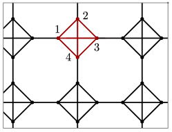
Figure 5: Lattice structure comprising four-site unit cells with all to all connection of uniform strength $a$ extended to a square lattice.

$$H= i\,a\left(\begin{matrix}0&1&1&1\cr-1&0&1&1\cr-1&-1&0&1\cr-1&-1&-1&0\end{matrix}\right)+i\left(\begin{matrix}0&0&e^{ik_{x}}&0\cr 0&0&0&e^{ik_{y}}\cr-e^{-ik_{x}}&0&0&0\cr 0&-e^{-ik_{y}}&0&0\end{matrix}\right).$$

The numerical brute force computation of Berry curvatures for this Hamiltonian reveals a sequence of six topological phase transitions at $a$-values $(\sqrt{2}-1,1,\sqrt{2}+1))=:(a_{-},1,a_{+})$ and the negative of these. Labeling the energy bands $1,2,3,4$ in ascending order in energy, we have $N=2$ occupied bands $n=1,2$ with a pattern of Chern numbers shown in Table 1: Starting from a topologically trivial phase at $a>a_{+}$, a phase transition involving bands $n=2,3$ at $a=a_{+}$ (see Fig. 6) defines the entry into a topological superconductor phase with $c=1$. At $a=1$, a phase transition involving the topological order of bands $1,2$ (and $3,4$) leads to a redistribution of band Chern numbers without changing the total topological index, $c$. Finally, at $a=a_{-}$, we have a transition back to $c=0$, however, this vanishing value is nontrivial in that it implies two bands with mutually canceling non-vanishing index, $c_{1}=1$ and $c_{2}=-1$.

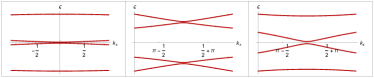
Figure 6: A cut at $k_{y}=0,\pi,\pi$ (left, center, right) through the two-dimensional dispersion relation at parameter values $a=a_{+}+0.3,b+0.04,a_{-}+0.02$ close to the topological phase transition points. Notice how the transition at $b$ involves the formation of a Dirac point between the occupied bands $c=1,2$.

To obtain an explicit low energy reduction of the system near, say, the critical point $a=a_{-}$, we verify that at the momentum hot-spot $k=(\pi,\pi)$ our Hamiltonian has two zero eigenvalue states,

$$v_{1} := \frac{1}{2}(-\sqrt{2},-1,0,1),$$ (18)

$$v_{2} := \frac{1}{2}(0,1,\sqrt{2},1).$$ (19)

Setting $a=a_{-}+{m}/({2(1+\sqrt{2})})$, and $k_{i}=\pi+q_{i}$, the two-band reduction, $H^{(2)}$, of the Hamiltonian obtained by projection onto the space spanned by $v_{1,2}$ assumes the form of the Haldane Haldane (1988) Chern insulator

$$H^{(2)}=-\frac{1}{2} \left(\sin(q_{2})\sigma_{3}+\sin(q_{1})\sigma_{1}\right.$$ (20)

$$+\left.(2+m-\cos(q_{1})-\cos(q_{2}))\sigma_{2}\right).$$

For $m>0$ and $m<0$, the two bands associated to this Hamiltonian carry winding (Chern) numbers $(0,0)$ and $(-1,1)$, respectively. The low energy Dirac approximation Eq. (17) (with $\kappa=-\frac{1}{2}$) is obtained by expansion in $q$ up to second order.

$a\in$	$(0,a_{-})$	$(a_{-},1)$	$(1,a_{+})$	$(a_{+},\infty)$
$c_{4}$	-1	-1	0	0
$c_{3}$	1	0	-1	0
$c_{2}$	-1	0	1	0
$c_{1}$	1	1	0	0
$c$	0	1	1	0

Table 1: Chern numbers carried by the four bands of the system for positive values of the parameter $a$. (The pattern is symmetric around $a=0$ and in this way can be extended to negative values.) The phase transitions changing the topological index, $c$, occur at $a_{\pm}$.

With these identifications, the equivalence between the TN and the SC is established, and from here one may — via the non-local boson-fermion mapping outlined in Section II — pass to the bosonic systems TC and IM. Notice how in our discussion of the fermion system, the emphasis shifted from real space to momentum space structures. Nevertheless, the full microscopic structure of the system remains under control, and this will become essential in the next section when we turn to the discussion of correlation functions.

IV Extension to inhomogeneous structures

So far, we have looked at the duality between our three systems in the translationally invariant case. However, they all show rich behavior when translational invariance is broken by domain walls or other defect structures, examples including vortices binding Majorana zero modes in the SC Fu and Kane (2008), non-local ‘disorder’ operators describing the correlations between endpoints of defect links in the IM Kadanoff and Ceva (1971), anyonic excitations as endpoints of error strings in the TC Kitaev (2003), or the long-rangedness of correlation functions at criticality (where we consider a correlation function as the result of an insertion of infinitesimally weak probing inhomogeneities.) The general duality must include a mapping between these defect structures, and their accompanying correlations. However, we anticipate that the passage from fermionic to bosonic systems involved in going from the SC to the IM or the TC will introduce an element of non-locality: the correlation between objects that are local in one setting may turn into the insertion of non-local string like objects in another.

These complications find their perhaps most vivid manifestation in the duality mapping of the simplest correlation function probing the superconductor, that between two Majoranas, Eq. (21) below. The dual representation of this function in the Ising context is famously complex Kadanoff and Ceva (1971); Dotsenko and Dotsenko (1983) and it involves the pairing of a spin and a disorder operator to a hybrid operator. The simultaneous appearance of a local (spin) and a non-local (disorder) operator reflects that we are representing the correlations of a fermion in the language of a bosonic model. Specifically, the spin-disorder dual of the Majorana correlation function responds sensitively to the relative placement of the two compound operators, as discussed in Ref. Kadanoff and Ceva (1971) and explored explicitly in a dual fermionic description in Ref. Dotsenko and Dotsenko (1983).

In the following, we show how the tensor network allows one to map defect structures and correlation functions with maximal explicitness. We will illustrate the construction on two examples. The first is the mapping of the above SC Majorana two-point correlation function. We will construct local pairs of spin and disorder operators as fractionalized representatives of the Majorana, and address the importance of their relative ordering on the lattice. The second example is motivated by the question what form these structures assume in the TC language. We find that for general parameter values the answer assumes the form of an exponentially decaying and not very illuminating ground state operator expectation value. However, the analysis of the latter becomes more rewarding once we introduce a spatial domain wall, i.e. an object which in superconductor language defines the surface of a topological insulator. In this case, our correlation function describes the spatial extension of a topological boundary mode, and we will discuss how this object turns into a non-decaying string operator expectation value in the toric code.

IV.1 Correlation functions

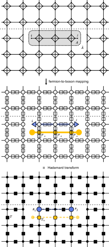
Figure 7: Top. Fermionic TN for $\langle\theta_{i}\theta_{j}\rangle$ divided into fermion parity even regions $A$ and $\bar{A}$. Center. The TN after fermion-to-boson mapping. We obtain a bosonic weighted $\mathbb{Z}_{2}$ TN with $\sigma_{z}$ matrices (transparent yellow squares) acting along a defect line on the dual lattice (yellow) and projections onto the state vector $\ket{1}$ at the sites $i$ and $j$, respectively. Bottom. The TN of the IM partition function obtained via a Hadamard gauge transformation. The $\sigma_{z}$-matrices are transformed to transfer matrices $T_{\text{DL}}$ of inverted coupling strengths $J\to-J$ (filled yellow squares) along the defect line and the spins at site $i$ and $j$ (blue dots) contribute a sign factor to the partition function leading to the expression in Eq. (24). The dashed gray line represents a (potential) boundary between regions of different $a$-values discussed in Sec. IV.2.

Correlation functions are described by a TN modified at the two points between which correlations are measured. These modifications can interfere with the fermionization procedure discussed in the previous section. Specifically, if the observables under consideration are of odd fermion parity, the mapping between bosonic and fermionic representations introduces a string-like object connecting the two point observables. To illustrate the principle – and to be entirely concrete – we start out from the fermionic two point correlation function

$$\langle\theta_{i}\theta_{j}\rangle:=\int(\mathrm{d}\theta)_{C}\,\theta_{i}\theta_{j}\,e^{\frac{1}{2}\theta^{T}(A+C)\theta}\;,$$ (21)

where $C$ denotes the signed adjacency matrix of the network and $A$ the collection of all matchgate tensor generating matrices. We may think of this as the contraction of a fermionic tensor network subject to two incisions as illustrated in Fig. 7. Doing the integral, we obtain

$$\langle\theta_{i}\theta_{j}\rangle\propto H^{-1}|_{ij}\;,$$ (22)

with the Hamiltonian $H=\mathrm{i}(A+C)$. Close to a critical point, e.g., $a=a_{-}$, $H$ can be approximated by the two-band Hamiltonian Eq. (17) linearized around $q_{x},q_{y}=0$. At criticality, $m=0$, the gap vanishes and the correlation function approaches an $l^{-1}$ power law where the exponent follows from dimensional analysis and $l$ is the distance between $i$ and $j$. However, in addition to this asymptotic distance behavior, we have additional short range lattice structures to consider. A single point $i=((x,y)b)$ is defined by unit cell coordinates $(x,y)$ and an intra-cell index $b=1,\dots,4$. It turns out that only pairs $i,j$ with select combinations of this data survive projection onto the two-band reduction, and hence are long-range correlated. For example, considering points separated along the $x$-direction, we find $\langle\theta_{(x,y)1}\theta_{(x+l,y)1}\rangle=0$, while $\langle\theta_{(x,y)1}\theta_{(x+l,y)3}\rangle\propto 1/l$.

Fermion boson mapping.

We next aim to represent this correlation function in the language of the bosonic TN. The challenge here is the presence of fermion parity odd tensors at sites $i$ and $j$. To deal with this situation, we decompose the tensor network into two parts which are individually fermion-parity even. The first of these, $A$, contains $\theta_{i}$ and $\theta_{j}$, and hence is fermion even in total. The complement, $\bar{A}$, contains the rest of the tensor network. For the sake of simplicity, we chose $A$ to be as small as possible, namely as a chain of tensors connecting sites $i$ and $j$ (see Fig. 7 top). Referring to Appendix A.1 for a more detailed discussion, the goal now is to contract all tensors in $A$ and reorder the fermionic modes into standard ordering. (The tensors of $\bar{A}$ can be assumed to be in standard ordering to begin with.) As a necessary byproduct, this operation introduces a string of fermion parity tensors between sites $i$ and $j$. In a final step, we contract the bosonic versions of $A$ and $\bar{A}$ to obtain a bosonic tensor network in standard ordering.

In bosonic language, the above parity string is expressed through $\sigma_{z}$-matrices acting on the virtual bonds of the TN (see Fig. 7 center). The $\theta$-modes themselves become projections onto spin-up, i.e., $\ket{1}$-state at sites $i$ and $j$. The resulting bosonic tensor network is shown in the middle panel of Fig. 7. Having defined two alternative representations of the TN subject to point sources at sites $i$ and $j$, we now turn to the interpretation of these structures in terms of condensed matter correlation functions.

SC: Eq. (21) affords an obvious interpretation as the Majorana ground state correlation function of a superconductor. Specifically, we think about the r.h.s. of Eq. (22) as the ground state, or zero energy, $\epsilon=0$, matrix element $G_{ij}$ of the resolvent $G=(\epsilon-H)^{-1}$. (Due to the presence of a spectral gap and the absence of convergence issues in the Majorana functional integral, it is not necessary to shift $\epsilon$ into the complex plane as for generic Green functions.) Its algebraic decay then reflects the long-range correlation of Majorana quasiparticles at the gap closing transition of the topological superconductor.

IM: Next, we interpret the bosonic incarnation of the sourced tensor network in terms of an Ising model correlation function. As before, we obtain the corresponding partition sum by performing a Hadamard transform (see Fig. 3) which in the presence of sources has the following effect: the $\ket{1}$-projections become projection to the $\ket{-}$-state, meaning, if the spin at position $i$ is up, we obtain a minus sign. The same holds for the spin at position $j$. We identify the parity string as a defect line (DL) and observe that the transfer matrices at all bonds crossed by that defect line are given by

$$T_{\text{DL}}=\sqrt{2}HW^{2}\sigma_{z}H=\frac{1}{\sqrt{2}}\begin{pmatrix}1-a&1+a\\ 1-a&1+a\end{pmatrix}\;.$$ (23)

Comparing this to the result in Eq. (11) and Eq. (12), we note that these are transfer matrices with inverted coupling strength, i.e., $T_{\text{DL}}=T_{J\to-J}$.

In summary, the tensor network after Hadamard transform shown at the bottom of Fig. 7 is a spin-spin correlation function of sites $i$ and $j$, but with a Hamiltonian $H_{\text{DL}}$ that has a modified coupling strength $J\mapsto-J$ along a defect line

$$Z_{\text{corr},ij}=\sum_{\{s_{i}\}=\pm 1}s_{i}s_{j}e^{-\beta H_{\text{DL}}(\{s_{i}\})}\;.$$ (24)

The specific path entering the construction of the defect line depends on the arbitrary choice made in dividing the tensor network into $A$ and $\bar{A}$.

These building blocks entering the construction of the Ising representation of the fermion correlation function have a long history of research. Specifically, $\sigma_{z}$ string line defects extending from a point of the lattice along arbitrary paths to infinity are called disorder operators and and have been introduced in Ref. Kadanoff and Ceva (1971). They owe their name to the fact that they assume finite expectation values in the disordered high-temperature phase of the IM, and they are related by (Kramers-Wannier) duality to the native local spin operators. Composite correlation functions involving pairs of disorder operators (now connected by a finite defect line) and spin operators were considered in the same reference, where the importance of the precise relative positioning of spin and disorder operator (addressed above in the language of the Majorana representation) was discussed. In a lattice construction conceptually close to the present one but formulated directly with the framework of the IM, Ref. Dotsenko and Dotsenko (1983) investigated the braiding properties of the composite operator to demonstrate that it defines an effective (Majorana fermion). Within our present construction the bridge between free Majorana fermions and composite IM operators is established in the explicit and arguably maximally concise mapping of the fermionic to the bosonic TN.

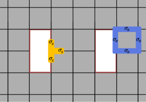
Figure 8: Toric code with smooth boundaries. The Hamiltonian in the bulk (shaded in grey) is given by the conventional square lattice Hamiltonian. Along the boundary all vertex operators are modified such that they are given by a product of $\sigma_{z}$-matrices acting on the edges inside the grey shaded region only. The plaquette operators remain the same.

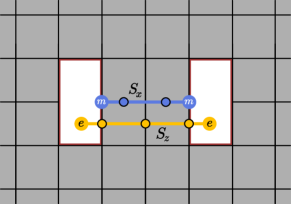
Figure 9: Toric code with smooth boundaries around two holes that arise from the correlation function ‘incisions’ at sites $i$ and $j$ (cf. Fig. 7 center). The string of $\sigma_{x}$-matrices, $S_{x}$ (blue), creates parity violations ($m$-excitations) at its end-points. The string of $\sigma_{z}$-matrices, $S_{z}$ (yellow), connects the incision sites and creates $e$-excitations at its endpoints.

TC: We finally turn to the an interpretation of the correlation function in terms of toric code ground state expectation values. To be more precise, we consider the bosonic TN in the middle panel of Fig. 7 and try to identify a toric code ground state $\ket{\Psi}$ such that $\braket{\Psi}{\ldots}{\Psi}$ corresponds to the given TN locally and the ellipses stand for appropriate operators to be identified as well. For general $a$-values, this procedure leads to complicated and not very revealing expressions. However, at the toric code fixed point, $a=1$, i.e. in the absence of string tension, the construction becomes straightforward. Focusing on this case, we note that for $a=1$ the weight matrices are identity matrices, meaning that we can omit them in the pictorial representation of the TN in the middle panel of Fig. 7.

We next note that the TN modified for the presence of source terms has a number of specific features which help to identify the state vector $\ket{\Psi}$ and the operators featuring in the expectation value. First, it is missing a bond to the left (right) of site $i$ ($j$). This missing bond suggests to choose $\ket{\Psi}$ as the ground state vector of the toric code with holes at sites $i$ and $j$. In the context of the toric code, the minimal surface bounding these holes is known as a smooth boundary. The ground state of a toric code containing smooth boundaries is a superposition of all closed loops of spin-up states , where the loops are allowed to include boundary links (cf. Fig. 8). The remaining features of the TN we need to reproduce are the string of sign flips along the defect line, and the $\ket{1}$-projections at sites $i$ and $j$.

The constructive modeling of these structures is a nice illustration of tensor network constructions and detailed in App. C. We here simply state the result and note that the state we are looking for is $\ket{\Psi}:=S_{x}\ket{\Psi_{\square}}$, where $\ket{\Psi_{\square}}$ is the ground state of the TC with smooth boundaries mentioned above and $S_{x}=\sigma_{x}\otimes\ldots\otimes\sigma_{x}$ is a string of $\sigma_{x}$-matrices (bit flips) between sites $i$ and $j$. Applied to the ground state, this operator generates an excited state with two $m$-anyons located at the endpoints of the string (cf. Fig. 9) Kitaev (2003). The overlap $\braket{S_{x}\Psi_{\square}}{S_{x}\Psi_{\square}}$ reproduces the $\ket{1}$-projection of the TN in the middle panel of Fig. 7.

The sought after operator replacing the ellipses in $\braket{\Psi}{\ldots}{\Psi}$ is $S_{z}=\sigma_{z}\otimes\ldots\otimes\sigma_{z}$ – a string of $\sigma_{z}$-matrices (phase flips) along a path connecting sites $i$ and $j$ on the dual lattice. This operator is known to generate an excited state with $e$-anyons at its endpoint (cf. Fig. 9) Kitaev (2003). Here, the $e$-anyons lie inside the two holes with smooth boundary and instead give rise to another (orthogonal) ground state of the Hamiltonian with smooth boundary. The expectation value of this operator for a TC ground (or excited) state reproduces the string of sign flips in the TN.

In summary, the expectation value reducing to the TN in the middle panel of Fig. 7 and satisfying the above locality condition is given by $\braket{\Psi}{S_{z}}{\Psi}=\braket{S_{x}\Psi_{\square}}{S_{z}}{S_{x}\Psi_{\square}}$. Since the support of $S_{x}$ and $S_{z}$ can be chosen to be non-overlapping, these two operators commute. With $S_{x}^{2}=\mathbb{1}$, we find $\braket{\Psi}{S_{z}}{\Psi}=\braket{\Psi_{\square}}{S_{z}\Psi_{\square}}$.

Let us discuss this result. We have seen that the presence of the $S_{x}$ strings is irrelevant in the expectation values. The job of these operators was to implement the $\ket{1}$-projections, which in turn were dual to the spin operators in the Ising context. Since $a=1$ translates to $J\beta=\infty$ (cf. Eq. (12)) this dual IM is deeply within the ferromagnetic phase, where spins are uniformly aligned and hence drop out of correlation functions. We next note that the operator $S_{z}$ applied to the ground state generates a state with two $e$-anyons at its endpoints. This state is orthogonal to the state $\ket{\Psi_{\square}}$ and the overlap $\braket{\Psi_{\square}}{S_{z}\Psi_{\square}}$ is trivially zero. This, again, is expected by duality – the $S_{z}$ operator corresponds to the disorder correlation function in the IM which vanishes in the ferromagnetic phase.

We thus conclude that all the so far effort has led to the dual TC representation of a trivially vanishing correlation function. This vanishing is due to the fact that we are considering correlations on top of a bulk background which, for $a=1$, is fully gapped. However, the situation becomes more interesting, when we allow for the presence of a system boundary spatially aligned to our probe operators.

IV.2 Boundary phenomena

Turning back to the TN, assume a separation of our system into a ‘topological’ region, $R$ defined by a value $a>a_{-}$ of the coupling constant, and a ‘non-topological’ complement with $a<a_{-}$. In SC language, this will define an interface between a topological and a non-topological superconductor, which we know supports gapless Majorana boundary modes. On this basis, we anticipate that the TC representation, too, will support long range correlations, which we can probe by putting two observation points $i$ and $j$ next to it. This is the setup considered in the following.

Consider the TN in the middle panel of Fig. 7 where now the weight matrices above the dashed line have $a<a_{-}$. For simplicity, we set $a=0$, which reduces these matrices to projections onto the state vector $\ket{0}$. Below the dashed line, where $a>a_{-}$, we choose $a=1$, implying that the weights become unit matrices. In effect, this network has all bonds above the dashed line, including those that are crossed by it, removed. This defines a maximally simple interface between a topological region and ‘vacuum’.

TN: In TN language, the above construction introduces another smooth boundary along the interface, in addition to that surrounding the correlation function observation points. As before, we aim to identify the correlation function generalized for the presence of the interface with a suitable ground state expectation value. Reconsidering the construction in the previous section, we conclude that it remains unchanged, only that the ground state in question now is that of the system with the generalized boundary, $\ket{\Psi_{\square,|}}$. In the expectation value , the $S_{x}$ string is irrelevant as before, leading to .

So far, we have not specified the positioning of the sites $i$ and $j$ relative to the boundary. The situation gets interesting when they come close to it (as depicted in the middle panel of Fig. 7). Once they touch, the holes surrounding $i$ and $j$ are ’cut open’ and partially lie outside the bulk. This has a dramatic effect. While previously, we found that $\braket{\Psi_{\square}}{S_{z}}{\Psi_{\square}}=0$, we now find that $\braket{\Psi_{\square}}{S_{z}}{\Psi_{\square}}=1$. This follows from the fact that the $e$-excitation at the end of the $S_{z}$ string are no longer trapped in the bulk, instead, they lie outside of the bulk region and by using a sequence of straightforward TN manipulation (cf. identity (4) in Fig. 17), we can remove them entirely from the system. The intuition behind this construction is illustrated in Fig. 10.

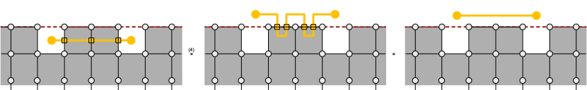
Figure 10: Deforming and removing a $S_{z}$-string at a smooth boundary by repeated application of identity (4) from Fig. 17.

V Summary and discussion

In this work, we have considered three reference systems which are individually of outstanding importance to condensed matter research: the toric code as an exactly solvable model of long range entangled matter, the class D superconductor as an example of a topological insulator, and the two-dimensional Ising model as a maximally simple proxy for systems with a discrete symmetry breaking phase transition. These three system classes are dual to each other. More precisely, the duality connects the ground states of the TC and the SC with the partition sum of the IM. Being exact, it extends to all phenomena displayed by the three partner systems, including their topological or thermal phase transitions, the buildup of algebraic correlations at criticality, and the presence of topological boundary modes at domain walls. These equivalences are remarkable in that they connect phenomena conventionally addressed in different hemispheres of physics — such as the phase transition between a spin polarized phase and a topological spin liquid vs. the band closing transition between a trivial and a topological superconductor.

The dualities discussed in this work are largely known in principle, and have been derived in previous work by different methods. As they include the duality between fermionic and bosonic systems, a standard approach is to take a detour via a transient mapping to one dimensional quantum systems, for which Bose–Fermi duality is established by Jordan-Wigner transformation. An alternative approach is to look at them through the coarse graining lens of CFT and establish equalities between differently realized operators in, say, the Ising and the free Majorana CFT at criticality. These approaches illustrate the principle, but arguably lack in the microscopic resolution required when it comes to the precise comparison of correlation functions. To the best of our knowledge, this point has first been made in Ref. Dotsenko and Dotsenko (1983), an observation being that, e.g., the free Majorana correlation function in the SC becomes that between a spin and a disorder composite operator in the IM where the exact positioning of the two compound operators on the lattice becomes crucial. That reference has solved the problem by staying on the two dimensional lattice and employing (string-) operator algebra to demonstrate that the spin-disorder operator satisfies the commutation relations of a Majorana fermion.

In this work, we have proposed an alternative and more comprehensive approach to the duality, the key idea being to use a tensor network as an intermediate. While at first sight a formulation introducing a fourth player into a situation that looks complicated already may not look appealing, engaging a translator TN has various advantages. First, the TN comes in two incarnations a bosonic and a fermionic one, the passage between the two being explicit, with no dimensional detours required. Second, both realizations of the TN are elementary. Being bond dimension two networks, the compound tensors involved in the construction of the net assume the form of $2\times 2$ matrices, binary Kronecker $\delta$’s and $\mathbb{Z}_{2}$-parity projection tensors. After passing through a mild learning curve, one can use powerful graphical relations of tensor algebra as a resource to obtain results which arguably assume a substantially more complicated and tedious form in different formulations. Another attractive feature is that the fermionic TN assumes the form of a Gaussian Majorana integral. As an alternative to using tensor relations, one may proceed via techniques otherwise employed in the analysis of free fermion systems, an approach naturally relevant to the understanding of the superconductor. In this way, we not only bridge different frameworks within a single formalism, but also the mindsets of different scientific communities.

While the present work has focused on known manifestations of the duality in the focus of attention, there are several obvious extensions into less charted territory. The first is a generalization to non-translationally invariant systems which, depending on the context, means bit errors, random magnetic exchange, or static impurities. The tensor network construction has no issues with the presence of spatially fluctuating bonds, and a natural approach will be to perform ensemble averaging directly on the level of the TN to generalize the latter to an effective continuum field theory Wille et al. (2023b). Other generalizations include the addition of nonlinear contributions to the TN, asking if they, too, afford a condensed matter interpretation. One may also study geometric deformations of the TN, for instance the hyperbolic geometries entering the construction of holographic networks. Here again, it is natural to ask if and how the holographic bulk boundary correspondence manifests itself in the dual system classes.

VI Acknowledgements

We acknowledge support from the Deutsche Forschungsgemeinschaft (DFG) under Germany’s Excellence Strategy Cluster of Excellence Matter and Light for Quantum Computing (ML4Q) EXC 2004/1 390534769 (A.A.) and within the CRC network TR 183 (project grant 2777101999) as part of projects B04 (A.A and J.E.). It has also received funding from Germany’s Excellence Strategy Cluster of Excellence MATH+ (J.E.) and the BMBF (RealistiQ). C.W. acknowledges support from the European Research Council under the European Union Horizon 2020 Research and Innovation Programme via Grant Agreement No. 804213-TMCS.

Appendix A Mapping bosonic to fermionic tensor networks

In the following, we discuss how the map from bosonic to fermionic tensors behaves under tensor contraction. In particular, we investigate under which conditions the diagram in Fig. 11 is commutative or almost commutative in a sense to be specified momentarily. We recapitulate that we need to choose an orientation for the contraction of the fermionic bonds and an ordering of the contracted bosonic tensor for their fermionization. We will focus on rectangular tensor network patches on a square lattice and show that a particular choice of orientations and orderings yields consistent results.

The assignments are as follows. We fix the orientation of all fermionic bonds to be left to right for horizontal links and top to bottom for vertical links. We define the index ordering of the tensors to be clockwise with the start point at the top most index along the left edge (cf. Fig. 12). We refer to this pattern as standard ordering. With this choice, the fermionized contracted bosonic tensor network is identical to the contraction of the tensors fermionized individually up to a correction of sign factors that depends solely on the fermion parities of the fermionic modes at the left boundary of the patch.

To see this, we consider the initial ordering or all fermionic modes in the uncontracted tensor networks $\mathcal{O}_{\text{initial}}$ and perform a particular reordering to the ordering $\mathcal{O}_{\text{rect}}$. This produces a sign factor $S=(-1)^{\sigma(\mathcal{O}_{\text{initial}},\mathcal{O}_{\text{rect}})}$. We show that $\mathcal{O}_{\text{rect}}$ is compatible with the contraction of fermionic bonds, i.e., we can readily perform the integration over Grassmann variables and are left with a tensor that only has fermionic modes at its boundary. In particular the ordering of the boundary modes coincides with the standard ordering (see Fig. 13(d)). We evaluate the sign factor $S$ (see Fig. 13(e) and find that it only depends on the fermionic parities of the fermionic modes at the left boundary of the patch.

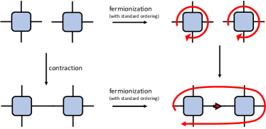
Figure 11: Tensor contraction versus fermionization. The diagram is non-commutative in general. During the fermionization process, we need to choose an ordering of the fermionic modes. We always choose so-called standard ordering defined in the main text. For the fermionic contraction, we need to choose a bond orientation and again choose a standard orientation.

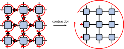
Figure 12: Contraction of fermionic tensors. The contracted tensor can be brought into standard ordering at the cost of introducing a sign-correction indicated by the red dots corresponding to matrices $s_{ij}=(-1)^{|j|}\delta_{ij}$.

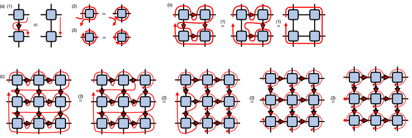
Figure 13: (a) Identities for contracting and re-ordering fermionic modes. (1) Contraction of a fermionic bond. If the modes to be contracted (red arrow) occur in consecutive order in the ordering of all fermionic modes (red line) they can be integrated out and removed from the tensor network. (2) Manipulating the ordering of fermionic modes. The total fermion parity of the tensors is even. Thus, when the ordering string ‘encircles’ a tensor, we can decouple it from the ordering string. (3) Cyclic permutation of the fermionic modes of a parity even tensor according to $\theta_{2}^{j}\theta_{3}^{k}\theta_{4}^{l}\theta_{1}^{i}=(-1)^{i}\theta_{1}^{i}\theta_{2}^{j}\theta_{3}^{k}\theta_{4}^{l}$ yields a sign factor $(-1)^{i}$ represented as a red dot. (b) A tensor network with ordering $\mathcal{O}_{\text{rect}}$. Fermionic bonds are integrated out sequentially using rule (1) to arrive at a fully contracted network with boundary modes ordered in standard ordering. (c) Calculating the sign factor $\sigma(\mathcal{O}_{\text{rect}},\mathcal{O}_{\text{initial}})$. We deform the global ordering string according to rule (2) several times. In the last equality we use the cyclic permutation rule (3) to obtain the initial ordering. In this process we obtain the sign factor represented by the red dots along the left edge of the network.

A.1 Fermion to Boson mapping for correlation functions

We now describe the steps of the mapping in more detail. On a square lattice (cf. Fig. 14), the product of a single 4-leg matchgate tensor and a pre-exponential $\theta$ factorizes into a 3-leg matchgate tensor and a single $\theta$ as illustrated by the example

$$e^{\frac{1}{2}\theta_{i}a_{ij}\theta_{j}}\theta_{3}=(1+a_{12}\theta_{1}\theta_{2}+a_{14}\theta_{1}\theta_{4}+a_{24}\theta_{2}\theta_{4})\theta_{3}\;.$$ (25)

Figure 14: Region $A$ of the tensor network, containing the individual modes $\theta_{i}$ and $\theta_{j}$ and a string of connecting tensors such that the total parity of $A$ is even. Left: Division of the region $A$ into two parity odd patches (ordered). The first patch is contracted and emerges with standard ordering. The second one is given by the single mode $\theta_{j}$. Right: The contraction of the two patches emerges with non-standard ordering. Reordering it to standard-ordering brings about a string of sign factors along the modes at the bottom.

We next divide the tensor network into the parts $A$ and $\bar{A}$ as indicated above (cf. Fig. 7) and contract the tensor network $A$. Part $A$ is the interesting part and is itself composed of fermion-parity even tensors and two fermion-parity odd tensors whose ordering has to be stated explicitly (as they do not commute). The ordering is inherited from the definition of the correlation function, here it is $\theta_{i}\theta_{j}$. A convenient partitioning of $A$ is to split-off $\theta_{j}$ from the rest. Everything but $\theta_{j}$ can be contracted as usual and gives rise to a tensor with fermionic modes in standard ordering. In our case, this is a clockwise orientation with starting point on the top-most edge on the left side of the patch.

We now only need to contract the remaining $\theta_{j}$ mode with the rest and reorder the product to standard ordering. To do so, we need to move $\theta_{j}$ past all fermionic modes such that standard ordering is reached. In the example in Fig. 7 this corresponds to moving $\theta_{j}$ past all modes on the bottom segment of the already contracted strip. This induces a sign factor depending on the fermion parity of the corresponding edges as indicated by yellow dots in the figure. With the standard ordering and even-parity in place we can now transform the tensor network to a bosonic tensor network as before and rewrite it as a weighted $\mathbb{Z}_{2}$-tensor network.

Appendix B Class D topological superconductors

B.1 Band structure, topological invariants, and Dirac representation

The Bogoliubov-de Gennes Hamiltonian of spin-triplet superconductor in the absence of time reversal invariance (the defining signatures of symmetry class D) is conventionally represented as

$$\hat{H}:=(C^{\dagger},C)\left(\begin{array}[]{cc}h&\Delta\\ \Delta^{\dagger}&-h^{T}\end{array}\right)\left(\begin{matrix}C\cr C^{\dagger}\end{matrix}\right)=:\psi^{\dagger}\tilde{H}\psi,$$ (28)

where $C=\{C_{i}\}$ is a vector of (spinless) lattice fermion creation operators, and $\Delta=-\Delta^{T}$ an anti-symmetric lattice order parameter. In this language, the class D symmetry of the matrix Hamiltonian $\tilde{H}$ assumes the form $H^{T}=-\sigma_{x}H\sigma_{x}$, the Pauli matrix acting in particle-hole space. From here, we may pass to a real (‘Majorana’) representation via unitary transformation

$$\psi=\left(\begin{matrix}C\cr C^{\dagger}\end{matrix}\right):=\frac{1}{\sqrt{2}}\left(\begin{matrix}\eta+i\nu\cr\eta-i\nu\end{matrix}\right)=:U\Theta,$$ (29)

with $\Theta=(\eta,\nu)^{T}$, and $U=\frac{1}{\sqrt{2}}\left(\begin{smallmatrix}1&i\cr 1&-i\end{smallmatrix}\right)$. A quick calculation shows that in this Majorana representation our Hamiltonian assumes the form $\hat{H}=i\Theta^{T}A\Theta$ with the real anti-symmetric matrix

$$A=\left(\begin{matrix}-ih_{A}-i\Delta_{+}&h_{S}-\Delta_{-}\cr-h_{S}+\Delta_{-}&-ih_{S}+i\Delta_{+}\end{matrix}\right),$$ (30)

$$h_{S/A}=\frac{1}{2}(h\pm h^{T}),\qquad\Delta_{\pm}=\frac{1}{2}(\Delta\pm\Delta^{\dagger}).$$ (31)

Conversely, any even-dimensional anti-symmetric matrix may be represented in the block form Eq. (30), and in this way one may pass from the complex Bogoliubov-de Gennes representation to the Majorana representation, and back.

According to the general classification of topological insulators and superconductors, the two-dimensional superconductor in class D is a Chern insulator, carrying a $\mathbb{Z}$-valued topological index $c$. This index is in turn obtained by summation $c=\sum_{n=1}^{N}c_{n}$ over Chern numbers carried by individual Bloch bands, $n=1,\dots,N$, with band energies below the superconductor band gap at $\epsilon=0$. (Recall that single particle energies of a superconductor occur in pairs $\pm\epsilon$, and that the presence of an order parameter generically implies a band gap around $\epsilon=0$.)

To compute the numbers $c_{n}$, we label the band eigenvectors as $|n,k\rangle$ in terms of their two-dimensional crystal momenta $k\in\mathbb{T}^{2}$ and define the Berry connection

$$a(n,k):=i\langle n,k|\mathrm{d}|n,k\rangle=i\langle n,k|\partial_{k^{i}}|n,k\rangle\mathrm{d}k^{i}$$ (32)

and its associated curvature

$$f(n,k):=\mathrm{d}a(n,k)=i(\partial_{k^{j}}\langle n,k|)(\partial_{k^{i}}|n,k\rangle)\mathrm{d}k^{j}\wedge\mathrm{d}k^{i}.$$ (33)

Integration of the latter over the Brillouin zone then yields the Chern numbers as

$$c_{n}:=\frac{1}{2\pi}\int_{\mathbb{T^{2}}}f(n,k).$$ (34)

One is often interested in detecting changes of topological invariants upon crossing a topological phase transition point, i.e., situations where the Chern numbers $(c_{n},c_{n+1})\to(c_{n}\pm 1,c_{n+1}\mp 1)$ of two neighboring bands change via the transient appearance of a band gap closure at a Dirac point. The simplest possible case $(c_{n},c_{n+1})=(0,0)\to(\pm 1,\mp 1)$ may be conveniently described in terms of a minimal two-band reduction, where the Hamiltonian reduced to the two bands is described as a two-dimensional matrix Hamiltonian, $H_{k}^{(2)}:=\sum_{a=1}^{3}c_{a}(k)\sigma_{a}$, and the class D symmetry in Majorana representation

$$(H^{T})_{k}=H^{T}_{-k}=-H_{k}$$ (35)

requires $c_{1}(-k)=-c_{1}(k),c_{2}(k)=c_{2}(k),c_{3}(-k)=-c_{3}(k)$. In the vicinity of a phase transition point, the Hamiltonian reduces to the Hamiltonian Eq. (17). In this reduction, the above definition of Chern numbers counts the number of windings of the coefficient vector $(q_{1},q_{2},m+cq^{2})$ around the origin as a function of $q$. It is straightforward to verify that this criterion translates to the assignment of Chern numbers mentioned in the main text.

B.2 Majorana zero mode

We may upgrade our band insulator to one with a topologically degenerate ground space by adding $\mathbb{Z}_{2}$ vortices. Assuming a gauge where the entire $\pi$-flux carried by a half flux quantum vortex is picked up along one lattice bond, a $\mathbb{Z}_{2}$ vortex is realized by the insertion of a line defect along which the sign of the hopping amplitude is inverted, $1\to-1$. On the same basis, a vortex pair corresponds to a line defect of finite length. Now assume each of its two vortex centers to be surrounded by a region with $a>a_{+}$ in which the system is topologically trivial, or represents an effective vacuum. One may show (see Appendix B.2) that at the boundaries to the topologically non-trivial outer region with $a<a_{+}$ zero energy Majorana states, $\gamma$, forms. (While a finite vortex core region facilitates the identification of the edge mode, its size may be shrunk to zero without compromising the topologically protected Majorana state.) The two Majoranas bound by a vortex pair define a complex fermion state, $\psi$, whose occupation parity realizes the $\mathbb{Z}_{2}$ degeneracy of the bi-vortex ground state. While the vortices cannot be individually removed, one may ‘fuse’ them either by contracting the connecting string, or by extending the vortex disk areas. Depending on the occupation of the previously non-local fermion, one is then either left with a vacuum state, or with a local and gapped fermion, in accordance with the fusion rule $\gamma\otimes\gamma=1\oplus\psi$.

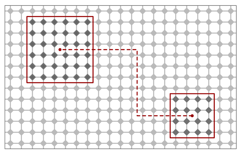
Figure 15: A pair of $\mathbb{Z}_{2}$ vortices realized by a string of sign inverted hopping amplitudes (bonds intersected by dashed line). At the interface between regions with $a>a_{+}$ (dark shaded) and $a<a_{+}$ (light shaded) zero energy Majorana edge modes form. The fusion of the two vortices leads to a topologically trivial configuration (equivalently, a $2\pi$-vortex)

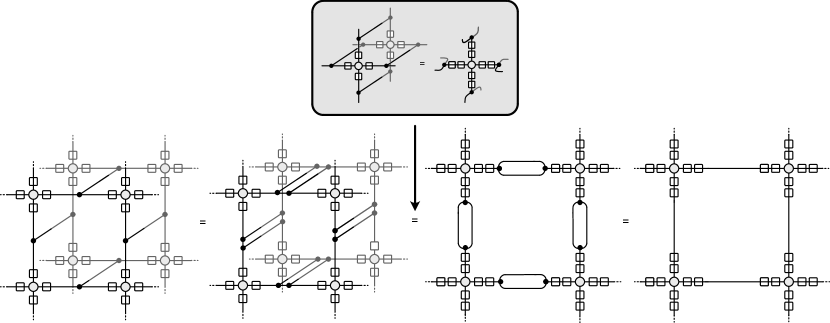
Figure 16: Collapsing the double layer $\braket{\Psi(t)}{\Psi(t)}$ TN to a single layer TN via a sequence of local deformations. All identities used follow from the definitions of the $\mathbb{Z}_{2}$- and the $\delta$-tensor in Fig. 3(b)

Vortex zero mode.

For completeness, we here demonstrate the formation of the vortex state and its zero mode by explicit computation. Assuming a core sufficiently large to admit a continuum representation in terms of the effective Hamiltonian Eq. (6), we consider a disk of radius $R$ with topological control parameter $m<0$ and $m>0$ inside and outside the disk perimeter. With $k_{i}=-i\partial_{i}$, and switching to polar coordinates we have $\partial_{1}=\cos\phi\partial_{r}-\frac{1}{r}\sin\phi\partial_{\phi}$ and $\partial_{2}=\sin\phi\partial_{r}+\frac{1}{r}\cos\phi\partial_{\phi}$. Using these identities, the Dirac Hamiltonian (with $\kappa=1$ for simplicity) assumes the form

$$H =i(\cos\phi\sigma_{1}+\sin\phi\sigma_{3})\partial_{r}+$$ (36)

$$\qquad\frac{i}{r}\left(-\sin\phi\sigma_{1}+\cos\phi\sigma_{3}\right)\partial_{\phi}+m(r)\sigma_{2}.$$ (37)

We are interested in the existence of zero mode solutions $H\psi=0$. The structure of the Hamiltonian suggests that it should be possible to apply a rotation around $\sigma_{2}$ to bring it to a simpler form. Specifically, consider the equivalent equation $\tilde{H}\tilde{\psi}=0$, with $\tilde{H}=UHU^{-1}$ and $\tilde{\psi}=U\psi$ where $U=\exp(-\frac{i}{2}\phi\sigma_{2})$. It is straightforward to verify that

$$\tilde{H}=i\left(\partial_{r}+\frac{1}{2r}\right)\sigma_{1}+\frac{i}{r}\partial_{\phi}\sigma_{3}+m(r)\sigma_{2}.$$

(Note: Naively, the second term in parentheses appears to violate Hermiticity. However, this is not so. It is actually required to make $i\left(\partial_{r}+\frac{1}{2r}\right)$ Hermitian w.r.t. the measure $rdr$ of polar integration.) Assuming $\phi$-independence of the zero mode, we are left with the equation

$$\left(\partial_{r}+\frac{1}{2r}-m(r)\sigma_{3}\right)\tilde{\psi}(r)=0.$$

Now decompose $|\tilde{\psi}\rangle=\psi_{+}|\uparrow\rangle+\psi_{-}|\downarrow\rangle$ in terms of eigenvectors of $\sigma_{3}$. This leads to

$$\left(\partial_{r}+\frac{1}{2r}\mp m(r)\sigma_{3}\right)\psi_{\pm}(r)=0,$$

with the solutions (pre-normalization)

$$\psi_{\pm}(r)=\left(\frac{R}{r}\right)^{1/2}\exp\left(\pm\int_{R}^{r}ds\,m(s)\right).$$

Since $m(r)>0$ for $r>R$, we retain $\psi_{-}$ as a normalizable option. Tidying up, we obtain

$$\psi(r,\phi)=\mathcal{N}\left(\frac{R}{r}\right)^{1/2}\exp\left(-\int_{R}^{r}ds\,m(s)\right)e^{i\frac{\phi}{2}}|\downarrow\rangle$$

for the zero mode of our system. At this point, it becomes clear why a (half-) vortex is required to realize this solution: the wave function as such obeys anti-periodic boundary conditions, $\psi(r,\phi+2\pi)=-\psi(r,\phi)$. Such states are not tolerated. However, if we assume $\pi$-flux inserted at the origin, the additional phase twist adds to that of $\tilde{\phi}$ to define a state with periodic boundary conditions. In the Majorana representation with its real anti-symmetric Hamiltonian, the $\pi$-flux insertion may be realized in terms of a line defect of bonds with sign inverted hopping amplitude as indicated in Fig. 15.

Appendix C Details on tensor network contractions for toric code ground states

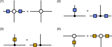
Figure 17: TN identities for the interaction of Pauli matrices $\sigma_{x}$ (blue square) and $\sigma_{z}$ (yellow square) with $\mathbb{Z}_{2}$-tensors (grey circles) and $\delta$-tensors (black circles). (1) A pair of $\sigma_{x}$-matrices applied to any pair of indices can be absorbed by a $\mathbb{Z}_{2}$-tensor. (2) The same holds for $\sigma_{z}$-matrices and $\delta$-tensors which is equivalent to identity (3). A string of $\sigma_{x}$($\sigma_{z}$)-matrices can be pulled through a $\delta$($\mathbb{Z}_{2}$)-tensor as shown in identities (2) and (4).

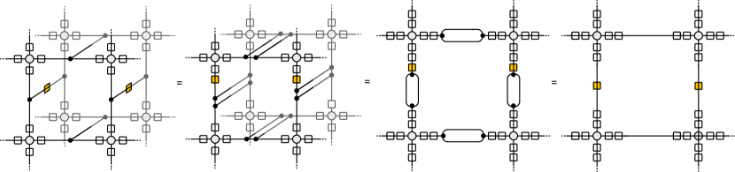
Figure 18: The overlap $\braket{\Psi(t)}{S_{z}}{\Psi(t)}$ reduced to a single layer MGTN with sign-string following the same reductions as in Fig. 16.

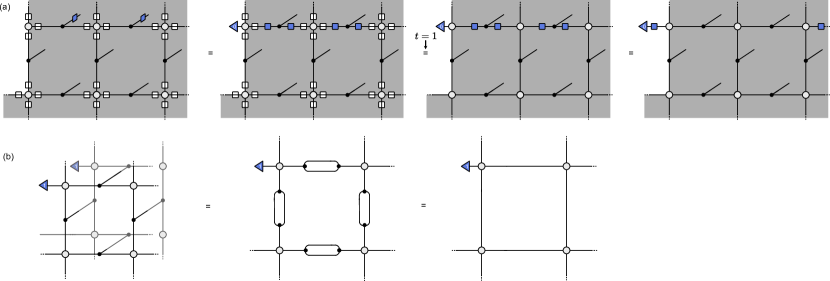
Figure 19: (a) Local patch of the state vector $S_{x}\ket{\Psi_{\square}}$. In the second equality we restrict to the fix-point, $t=1$. For $t\neq 1$, the non-commutativity of $\sigma_{x}$ and the weight-matrices obstructs the simple reduction procedure. (b) Contracting $\braket{S_{x}\Psi_{\square}}{S_{x}\Psi_{\square}}$ to a single layer TN.

In this appendix, we provide some details on tensor network contractions and identities used to derive results for the toric code ground state expectation values. The identity in Fig. 4(b) is derived using a sequence of local deformations shown in Fig. 16. Here, we use that $\delta$-tensors can be duplicated and that a local double layer patch can be reduced to a single layer patch as shown in the inset of the figure. Finally, we use that a loop of $\delta$-tensors can be contracted to an identity matrix as shown in the last equality.

Next, we provide further details on the interpretation of the TN representing a correlation function in Sec. III.2 Fig. 7 (center) as a ground state expectation value of the toric code in the case, where the parameter $a$ determining the weight matrices in the tensor network are $a=1$ inside and $a=0$ outside a region $R$.

In particular we show how a TN with a sign-string can be interpreted as $\braket{\Psi_{\square}}{S_{z}}{\Psi_{\square}}$ and how the TN with parity violations at sites $i$ and $j$ originating from the $\ket{1}$-state projections is given by $\braket{S_{x}\Psi_{\square}}{S_{x}\Psi_{\square}}$. All of these identifications are derived using the general rules for the ‘interaction’ of $\sigma_{x}$ and $\sigma_{z}$ matrices with $\mathbb{Z}_{2}$- and $\delta$-tensors shown in Fig. 17.

C.1 Sign string

Here, we show how the expectation value $\braket{\Psi_{\square}}{S_{z}}{\Psi_{\square}}$ is identified with a TN with a string of sign-flips (generated by $\sigma_{z}$-matrices) on the dual lattice. To see this consider Fig. 18. On the very left, we show a local patch of the double layer of $\ket{\Psi_{\square}}$ and $\bar{\Psi_{\square}}$ sandwiching a physical $\sigma_{z}$-error string. We again use a $\delta$-tensor doubling and then make use of the fact, that a $\sigma_{z}$ matrix can be moved through a $\delta$-tensor according to identity (3) in Fig. 17. After the contraction of the $\delta$-tensor loops, we obtain a purely virtual TN with the sign flip string as desired.

C.2 $\ket{1}$-projections and parity violations

In the main text, we have shown how the $\ket{1}$-projections can be gauged away. Here, we provide an alternative interpretation and show how the projections onto the $\ket{1}$-state can be interpreted as the overlap $\braket{S_{x}\Psi_{\square}}{S_{x}\Psi_{\square}}$ establishing a connection with the $m$-excitations in the toric code. We start by taking a closer look at the state vector $S_{x}\ket{\Psi_{\square}}$ and its tensor network representation in Fig. 19(a). By using identity (2) from Fig. 17 we can trade a $\sigma_{x}$-matrix acting on the physical index for two $\sigma_{x}$-matrices acting on the virtual level. We also note that a 3-leg $\mathbb{Z}_{2}$-tensor is identical to a 4-leg $\mathbb{Z}_{2}$-tensor with one index projected to the state vector $\ket{0}$ (first equality in Fig. 19(a)). Now, if we are working with a TC ground state with string tension ($a\neq 1$), we encounter the problem that the $\sigma_{x}$-matrices do not commute with the weight-matrices which obstructs further simplifications. However, at the fix-point ($a=1$), the weight matrices reduce to identity matrices (second equality in Fig. 19(a)). In this case, we can absorb pairs of $\sigma_{x}$-matrices at the $\mathbb{Z}_{2}$-tensors using identity (1) from Fig. 17. We are left with $\sigma_{x}$-matrices acting on the $\ket{0}$-states at the end of the string $S_{x}$ which give rise to the $\ket{1}$-state projections we set out to identify.

Now, we consider the overlap $\braket{S_{x}\Psi}{S_{x}\Psi}$ and show that it gives rise to a single layer TN with $\ket{1}$-projections at the end of the $S_{x}$-string. A local patch of the double layer TN around site $i$ is shown in Fig. 19(b). In analogy to the reductions in Fig. 16, we can reduce the TN to a single layer TN with $\ket{1}$-projections at the site $i$.

References

- Blackman (1982) J. A. Blackman, Phys. Rev. B 26, 4987 (1982).
- Blackman and Poulter (1991) J. A. Blackman and J. Poulter, Phys. Rev. B 44, 4374 (1991).
- Blackman et al. (1998) J. A. Blackman, J. R. Gonçalves, and J. Poulter, Phys. Rev. E 58, 1502 (1998).
- Berezin (1969) F. A. Berezin, Russ. Math. Surv. 24, 1 (1969).
- Plechko (1985) V. N. Plechko, Th. Math. Phys. 64, 748–756 (1985).
- Dotsenko and Dotsenko (1983) V. S. Dotsenko and V. S. Dotsenko, Adv. Phys. 32, 129 (1983).
- Merz and Chalker (2002) F. Merz and J. T. Chalker, Phys. Rev. B 65, 054425 (2002).
- Castelnovo and Chamon (2008) C. Castelnovo and C. Chamon, Phys. Rev. B 77, 054433 (2008).
- Zhu and Zhang (2019) G.-Y. Zhu and G.-M. Zhang, Phys. Rev. Lett. 122, 176401 (2019).
- Kitaev (2003) A. Y. Kitaev, Ann. Phys. 303, 2 (2003).
- Ryu et al. (2010) S. Ryu, A. P. Schnyder, A. Furusaki, and A. W. W. Ludwig, New J. Phys. 12, 065010 (2010).
- Onsager (1944) L. Onsager, Phys. Rev. 65, 117 (1944).
- Kaufman (1949) B. Kaufman, Phys. Rev. 76, 1232 (1949).
- Schultz et al. (1964) T. D. Schultz, D. C. Mattis, and E. H. Lieb, Rev. Mod. Phys. 36, 856 (1964).
- Vanhove et al. (2018) R. Vanhove, M. Bal, D. J. Williamson, N. Bultinck, J. Haegeman, and F. Verstraete, Phys. Rev. Lett. 121 (2018), 10.1103/physrevlett.121.177203.
- Aasen et al. (2020) D. Aasen, P. Fendley, and R. S. K. Mong, “Topological defects on the lattice: Dualities and degeneracies,” (2020), arXiv:2008.08598 [cond-mat.stat-mech] .
- Lootens et al. (2023) L. Lootens, C. Delcamp, G. Ortiz, and F. Verstraete, PRX Quantum 4 (2023), 10.1103/prxquantum.4.020357.
- Lootens et al. (2022) L. Lootens, C. Delcamp, and F. Verstraete, “Dualities in one-dimensional quantum lattice models: topological sectors,” (2022), arXiv:2211.03777 [quant-ph] .
- Valiant (2002) L. G. Valiant, SIAM J. Comp. 31, 1229 (2002).
- Bravyi (2009) S. Bravyi, Adv. Quant. Comp. 482, 179 (2009).
- Jahn et al. (2019) A. Jahn, M. Gluza, F. Pastawski, and J. Eisert, Science Adv. 5, eaaw0092 (2019).
- Cai and Choudhary (2006) J.-Y. Cai and V. Choudhary, in Theory and Applications of Models of Computation, edited by J.-Y. Cai, S. B. Cooper, and A. Li (Springer Berlin Heidelberg, Berlin, Heidelberg, 2006) pp. 248–261.
- Cai et al. (2007) J.-Y. Cai, V. Choudhary, and P. Lu, Th. Comp. Syst. 45, 108 (2007).
- Derby et al. (2021) C. Derby, J. Klassen, J. Bausch, and T. Cubitt, Phys. Rev. B 104, 035118 (2021).
- Kadanoff and Ceva (1971) L. P. Kadanoff and H. Ceva, Phys. Rev. B 3, 3918 (1971).
- Fradkin (2017) E. Fradkin, Journal of Statistical Physics 167, 427 (2017).
- Cirac et al. (2021) J. I. Cirac, D. Perez-Garcia, N. Schuch, and F. Verstraete, Rev. Mod. Phys. 93, 045003 (2021).
- Wille et al. (2023a) C. Wille, J. Eisert, and A. Altland, “In preparation,” (2023a).
- Wille et al. (2023b) C. Wille, J. Eisert, A. Jahn, and A. Altland, “In preparation,” (2023b).
- Orús (2014) R. Orús, Ann. Phys. 349, 117 (2014).
- Eisert et al. (2010) J. Eisert, M. Cramer, and M. B. Plenio, Rev. Mod. Phys. 82, 277 (2010).
- Bridgeman and Chubb (2017) J. C. Bridgeman and C. T. Chubb, J. Phys. A 50, 223001 (2017).
- Orús (2019) R. Orús, Nature Rev. Phys. 1, 538 (2019).
- Barthel et al. (2009) T. Barthel, C. Pineda, and J. Eisert, Phys. Rev. A 80, 042333 (2009).
- Corboz et al. (2010) P. Corboz, R. Orus, B. Bauer, and G. Vidal, Phys. Rev. B 81, 165104 (2010).
- Pižorn and Verstraete (2010) I. Pižorn and F. Verstraete, Phys. Rev. B 81, 245110 (2010).
- Kraus et al. (2010) C. V. Kraus, N. Schuch, F. Verstraete, and J. I. Cirac, Phys. Rev. A 81, 052338 (2010).
- Gu et al. (2010) Z.-C. Gu, F. Verstraete, and X.-G. Wen, “Grassmann tensor network states and its renormalization for strongly correlated fermionic and bosonic states,” (2010), arXiv:1004.2563 .
- Bultinck et al. (2017) N. Bultinck, D. J. Williamson, J. Haegeman, and F. Verstraete, J. Phys. A 51, 025202 (2017).
- Wille et al. (2017) C. Wille, O. Buerschaper, and J. Eisert, Phys. Rev. B 95, 245127 (2017).
- Note (1) For example, for tensors with four indices, we observe that a matchgate tensor has six free parameters, whereas a weighted tensor has only four.
- Gogolin et al. (2004) A. O. Gogolin, A. A. Nersesyan, and A. M. Tsvelik, Bosonization and strongly correlated systems (Cambridge University Press, 2004).
- Kac and Ward (1952) M. Kac and J. C. Ward, Phys. Rev. 88, 1332 (1952).
- Hurst and Green (2004) C. A. Hurst and H. S. Green, J. Chem. Phys. 33, 1059 (2004).
- Cho and Fisher (1997) S. Cho and M. P. A. Fisher, Physical Review B 55, 1025 (1997).
- Read and Ludwig (2000) N. Read and A. W. W. Ludwig, Physical Review B 63 (2000), 10.1103/physrevb.63.024404.
- Gruzberg et al. (2001) I. A. Gruzberg, N. Read, and A. W. W. Ludwig, Phys. Rev. B 63, 104422 (2001).
- Jian et al. (2022) C.-M. Jian, B. Bauer, A. Keselman, and A. W. W. Ludwig, Phys. Rev. B 106, 134206 (2022).
- Note (2) We multiply each link by , where the in the numerator multiplies our and the ones in the denominator remove the factor of multiplying the central -tensors.
- Isakov et al. (2011) S. V. Isakov, P. Fendley, A. W. W. Ludwig, S. Trebst, and M. Troyer, Phys. Rev. B 83, 125114 (2011).
- Dennis et al. (2002) E. Dennis, A. Kitaev, A. Landahl, and J. Preskill, J. Math. Phys. 43, 4452 (2002).
- Verstraete et al. (2006) F. Verstraete, M. M. Wolf, D. Perez-Garcia, and J. I. Cirac, Phys. Rev. Lett. 96, 220601 (2006).
- Gu et al. (2009) Z.-C. Gu, M. Levin, B. Swingle, and X.-G. Wen, Phys. Rev. B 79, 085118 (2009).
- Schuch et al. (2010) N. Schuch, I. Cirac, and D. Perez-Garcia, Ann. Phys. 325, 2153 (2010).
- Haldane (1988) F. D. M. Haldane, Phys. Rev. Lett. 61, 2015 (1988).
- Fu and Kane (2008) L. Fu and C. L. Kane, Phys. Rev. Lett. 100, 096407 (2008).
- Note (3) By contrast, the ground state of a TC with rough boundaries where bonds poke into the vacuum contains strings ending there.