Deformable 3D Gaussians for High-Fidelity Monocular Dynamic Scene Reconstruction

Abstract

Implicit neural representation has paved the way for new approaches to dynamic scene reconstruction and rendering. Nonetheless, cutting-edge dynamic neural rendering methods rely heavily on these implicit representations, which frequently struggle to capture the intricate details of objects in the scene. Furthermore, implicit methods have difficulty achieving real-time rendering in general dynamic scenes, limiting their use in a variety of tasks. To address the issues, we propose a deformable 3D Gaussians Splatting method that reconstructs scenes using 3D Gaussians and learns them in canonical space with a deformation field to model monocular dynamic scenes. We also introduce an annealing smoothing training mechanism with no extra overhead, which can mitigate the impact of inaccurate poses on the smoothness of time interpolation tasks in real-world datasets. Through a differential Gaussian rasterizer, the deformable 3D Gaussians not only achieve higher rendering quality but also real-time rendering speed. Experiments show that our method outperforms existing methods significantly in terms of both rendering quality and speed, making it well-suited for tasks such as novel-view synthesis, time interpolation, and real-time rendering. Our code is available at https://github.com/ingra14m/Deformable-3D-Gaussians.

1 Introduction

High-quality reconstruction and photorealistic rendering of dynamic scenes from a set of input images is critical for a variety of applications, including augmented reality/virtual reality (AR/VR), 3D content production, and entertainment. Previously used methods for modeling these dynamic scenes relied heavily on mesh-based representations, as demonstrated by methods described in [9, 14, 18, 40]. However, these strategies frequently face inherent limitations, such as a lack of detail and realism, a lack of semantic information, and difficulties in accommodating topological changes. With the introduction of neural rendering techniques, this paradigm has undergone a significant shift. Implicit scene representations, particularly as implemented by NeRF [28], have demonstrated commendable efficacy in tasks such as novel-view synthesis, scene reconstruction, and light decomposition.

To improve inference efficiency in NeRF-based static scenes, researchers have developed a variety of acceleration methods, including grid-based structures [7, 46] and pre-computation strategies [52, 44]. Notably, by incorporating hash encoding, Instant-NGP [29] has achieved rapid training. In terms of quality improvement, mipNeRF [2] pioneered an effective anti-aliasing method, which was later incorporated into the grid-based approach by zipNeRF [4]. 3D-GS [15] recently extended the point-based rendering to efficient CUDA implementation with 3D Gaussians, which has enabled a real-time rendering while matches or even exceeds the quality of Mip-NeRF [2]. However, this method is designed for representing static scenes, and its highly customized CUDA rasterization pipeline diminishes its scalability.

Implicit representations have been increasingly harnessed for modeling dynamic scenes. To handle the motion part in a dynamic scene, entangled methods [43, 49] conditioned NeRF on a time variable. Conversely, disentangled methods [34, 30, 31, 23, 39] employ a deformation field to model a scene in canonical space by mapping point coordinates at a given time to this space. This decoupled modeling approach can effectively represent scenes with non-dramatic action variations. However, irrespective of the categorization, adopting an implicit representation for dynamic scenes often proves both inefficient and ineffective, manifesting slow convergence rates coupled with a marked susceptibility to overfitting. Drawing inspiration from seminal NeRF acceleration research, numerous studies on dynamic scene modeling have integrated discrete structures, such as voxel-grids [38, 11], or planes [36, 6]. This integration amplifies both training speed and modeling accuracy. However, challenges remain. Techniques leveraging discrete structures still grapple with the dual constraints of achieving real-time rendering speeds and producing high-quality outputs with adequate detail. Multiple facets underpin these challenges: Firstly, ray-casting, as a rendering modality, frequently becomes inefficient, especially when scaled to higher resolutions. Secondly, grid-based methods rely on a low-rank assumption. Dynamic scenes, in comparison to static ones, exhibit a higher rank, which hampers the upper limit of quality achievable by such approaches.

In this paper, to address the aforementioned challenges, we extend the static 3D-GS and propose a deformable 3D Gaussian framework for modeling dynamic scenes. To enhance the applicability of the model, we specifically focus on the modeling of monocular dynamic scenes. Rather than reconstructing the scene frame by frame [26], we condition the 3D Gaussians on time and jointly train a purely implicit deformation field with the learnable 3D Gaussians in canonical space. The gradients for these two components are derived from a customized differential Gaussian rasterization pipeline. Furthermore, to solve the jitter in temporal sequences during the reconstruction process caused by inaccurate poses, we incorporate an annealing smoothing training (AST) mechanism. This strategy not only improves the smoothness between frames in the time interpolation task but also allows for greater detail to be rendered.

In summary, the major contributions of our work are:

• A deformable 3D-GS framework for modeling monocular dynamic scenes that can achieve real-time rendering and high-fidelity scene reconstruction.

• A novel annealing smoothing training mechanism that ensures temporal smoothness while preserving dynamic details without increasing computational complexity.

• The first framework to extend 3D-GS for dynamic scenes through a deformation field, enabling the learning of 3D Gaussians in canonical space.

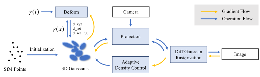
Figure 2: Overview of our pipeline. The optimization process begins with Structure from Motion (SfM) points derived from COLMAP or generated randomly, which serve as the initial state for the 3D Gaussians. We use the position (detached) of 3D Gaussians $\gamma(\operatorname{sg}(\bm{x}))$ and time $\gamma(t)$ with positional encoding as input to a deformation MLP network to obtain the offset $(\delta\bm{x},\delta\bm{r},\delta\bm{s})$ of dynamic 3D Gaussians in canonical space. We use a warm-up phase for the 3D Gaussians during the first 3k iterations without optimizing the deformation field. Following that, we use the fast differential Gaussian rasterization pipeline to perform joint optimization of the deformation field and the 3D Gaussians, as well as to adaptively control the density of the set of Gaussians.

2 Related Work

2.1 Neural Rendering for Dynamic Scenes

Neural rendering, due to its unparalleled capability to generate photorealistic images, has seen an uptick in scholarly interest. Recently, NeRF [28] facilitates photorealistic novel view synthesis through the use of MLPs. Subsequent research has expanded the utility of NeRF to various applications, encompassing tasks such as mesh reconstruction from a collection of images [45, 20], inverse rendering [5, 54, 25], optimization of camera parameters [21, 48, 47], and few-shot learning [10, 51].

Constructing radiance fields for dynamic scenes is a critical branch in the advancement of NeRF, with significant implications for real-world applications. A cardinal challenge in rendering these dynamic scenes lies in the encoding and effective utilization of temporal information, especially when addressing the reconstruction of monocular dynamic scenes, a task inherently involves sparse reconstruction from a single viewpoint. One class of dynamic NeRF approaches models scene deformation by adding time $t$ as an additional input to the radiance field. However, this strategy couples the positional variations induced by temporal changes with the radiance field, lacking the geometric prior information regarding the influence of time on the scene. Consequently, substantial regularization is required to ensure temporal consistency in the rendering results. Another category of methods [34, 30, 31] introduces a deformation field to decouple time and the radiance field, mapping point coordinates to the canonical space corresponding to time $t$ through the deformation field. This decoupled approach is conducive to the learning of pronounced rigid motions and is versatile enough to cater to scenes undergoing topological shifts. Other methods seek to enhance the quality of dynamic neural rendering from various aspects, including segmenting static and dynamic objects in the scene [39, 42], incorporating depth information [1] to introduce geometric prior, introducing 2D CNN to encode scene priors [22, 33], and leveraging the redundant information in multi-view videos [19] to set up keyframe compression storage, thereby accelerating the rendering speed.

However, the rendering quality of existing dynamic scene modeling based on MLP (Multilayer Perceptron) remains unsatisfactory. In this work, we will focus on the reconstruction of monocular dynamic scenes. We continue to decouple the deformation field and the radiance field. To enhance the editability and rendering quality of intermediate states in dynamic scenes, we have adapted this modeling approach to fit within the framework of differentiable point-based rendering.

2.2 Acceleration of Neural Rendering

Real-time rendering has long been a pivotal objective in the field of computer graphics, a goal that is also pursued in the domain of neural rendering. Numerous studies dedicated to NeRF acceleration have meticulously navigated the trade-off between spatial and temporal efficiency.

Pre-computed methods [12, 35] utilize spatial acceleration structures such as spherical harmonics coefficients [52] and feature vectors [13], cached or distilled from implicit neural representation, as opposed to directly employing the neural representations themselves. A prominent technique [8] in this category transforms NeRF scenes into an amalgamation of coarse meshes and feature textures, thereby enhancing rendering velocity in contemporary mobile graphics pipelines. However, this pre-computed approach may necessitate significant storage capacities for individual scenes. While it offers advantages in terms of inference speed, it demands protracted training durations and exhibits considerable overhead.

Hybrid methods [24, 27, 41, 7, 46, 4] incorporate a neural component within the explicit grid. The hybrid approaches confer the dual benefits of expediting both training and inference phases while producing outcomes on par with advanced frameworks [2, 3]. This is primarily attributed to the robust representational capabilities of the grid. This grid or plane-based strategy has been extended to the acceleration [11] or representation of time-conditioned 4D feature [38, 36, 6] in dynamic scene modeling and time-conditioned compact 4D dynamic scene modeling.

Recently, several studies [16, 53] have evolved the continuous radiance field from implicit representations to differentiable point-based radiance fields, markedly enhancing the rendering speed. 3D-GS [15] further innovates point-based rendering by introducing a customized CUDA-based differentiable Gaussian rasterization pipeline. This approach not only achieves superior outcomes in tasks like novel-view synthesis and scene modeling, but also facilitates rapid training times on the order of minutes, and supports real-time rendering surpassing 100 FPS. However, the method employs a customized differential Gaussian rasterization pipeline, which complicates its direct extension to dynamic scenes. Inspired by this, our work will leverage the point-based rendering framework, 3D-GS, to expedite both the training and rendering speeds for dynamic scene modeling.

3 Method

The overview of our method is illustrated in Fig. 2. The input to our method is a set of images of a monocular dynamic scene, together with the time label and the corresponding camera poses calibrated by SfM [37] which also produces a sparse point cloud. From these points, we create a set of 3D Gaussians $G(\bm{x},\bm{r},\bm{s},\sigma)$ defined by a center position $\bm{x}$, opacity $\sigma$, and 3D covariance matrix $\Sigma$ obtained from quaternion $\bm{r}$ and scaling $\bm{s}$. The view-dependent appearance of each 3D Gaussian is represented via spherical harmonics (SH). To model the dynamic 3D Gaussians that vary over time, we decouple the 3D Gaussians and the deformation field. The deformation field takes the positions of the 3D Gaussians and the current time $t$ as inputs, outputting $\delta\bm{x}$, $\delta\bm{r}$, and $\delta\bm{s}$. Subsequently, we put the deformed 3D Gaussians $G(\bm{x}+\delta\bm{x},\bm{r}+\delta\bm{r},\bm{s}+\delta\bm{s},\sigma)$ into the efficient differential Gaussian rasterization pipeline, which is a tile-based rasterizer that allows $\alpha$-blending of anisotropic splats. The 3D Gaussians and deformation network are optimized jointly through the fast backward pass by tracking accumulated $\alpha$ values, together with the adaptive control of the Gaussian density. Experimental results show that after 30k training iterations, the shape of the 3D Gaussians stabilizes, as does the canonical space, which indirectly proves the efficacy of our design.

Method	Hell Warrior			Mutant			Hook			Bouncing Balls
	PSNR$\uparrow$	SSIM$\uparrow$	LPIPS$\downarrow$	PSNR$\uparrow$	SSIM$\uparrow$	LPIPS$\downarrow$	PSNR$\uparrow$	SSIM$\uparrow$	LPIPS$\downarrow$	PSNR$\uparrow$	SSIM $\uparrow$	LPIPS$\downarrow$
3D-GS	29.89	0.9155	0.1056	24.53	0.9336	0.0580	21.71	0.8876	0.1034	23.20	0.9591	0.0600
D-NeRF	24.06	0.9440	0.0707	30.31	0.9672	0.0392	29.02	0.9595	0.0546	38.17	0.9891	0.0323
TiNeuVox	27.10	0.9638	0.0768	31.87	0.9607	0.0474	30.61	0.9599	0.0592	40.23	0.9926	0.0416
Tensor4D	31.26	0.9254	0.0735	29.11	0.9451	0.0601	28.63	0.9433	0.0636	24.47	0.9622	0.0437
K-Planes	24.58	0.9520	0.0824	32.50	0.9713	0.0362	28.12	0.9489	0.0662	40.05	0.9934	0.0322
Ours	41.54	0.9873	0.0234	42.63	0.9951	0.0052	37.42	0.9867	0.0144	41.01	0.9953	0.0093
	Lego			T-Rex			Stand Up			Jumping Jacks
Method	PSNR$\uparrow$	SSIM$\uparrow$	LPIPS$\downarrow$	PSNR$\uparrow$	SSIM$\uparrow$	LPIPS$\downarrow$	PSNR$\uparrow$	SSIM$\uparrow$	LPIPS$\downarrow$	PSNR$\uparrow$	SSIM $\uparrow$	LPIPS$\downarrow$
3D-GS	22.10	0.9384	0.0607	21.93	0.9539	0.0487	21.91	0.9301	0.0785	20.64	0.9297	0.0828
D-NeRF	25.56	0.9363	0.0821	30.61	0.9671	0.0535	33.13	0.9781	0.0355	32.70	0.9779	0.0388
TiNeuVox	26.64	0.9258	0.0877	31.25	0.9666	0.0478	34.61	0.9797	0.0326	33.49	0.9771	0.0408
Tensor4D	23.24	0.9183	0.0721	23.86	0.9351	0.0544	30.56	0.9581	0.0363	24.20	0.9253	0.0667
K-Planes	28.91	0.9695	0.0331	30.43	0.9737	0.0343	33.10	0.9793	0.0310	31.11	0.9708	0.0468
Ours	33.07	0.9794	0.0183	38.10	0.9933	0.0098	44.62	0.9951	0.0063	37.72	0.9897	0.0126

Table 1: Quantitative comparison on synthetic dataset. We compare our method to several previous approaches: 3D-GS [15], D-NeRF [34], TiNeuVox [11], Tensor4D [38] and K-Planes [36] on full resolution (800x800) test images. This may cause some methods to perform worse than the original paper because they downsample images by default. We report PSNR, SSIM, LPIPS(VGG) and color each cell as best, second best and third best. It is worth noting that we observed a discrepancy in the scenarios presented in the training and test sets of the Lego in D-NeRF dataset. This can be substantiated by examining the flip angles of the Lego shovels. To ensure a meaningful comparison, we opted to utilize the validation set of Lego as the test set in our experiments. See more in supplementary materials.

3.1 Differentiable Rendering Through 3D Gaussians Splatting in Canonical Space

To optimize the parameters of 3D Gaussians in canonical space, it is imperative to differentially render 2D images from these 3D Gaussians. In this work, we employ the differential Gaussian rasterization pipeline proposed by [15]. Following [55], the 3D Gaussians can be projected to 2D and rendered for each pixel using the following 2D covariance matrix $\Sigma^{\prime}$:

$$\Sigma^{\prime}=JV\Sigma V^{T}J^{T},$$ (1)

where $J$ is the Jacobian of the affine approximation of the projective transformation, $V$ symbolizes the view matrix, transitioning from world to camera coordinates, and $\Sigma$ denotes the 3D covariance matrix.

To make learning the 3D Gaussians easier, $\Sigma$ is divided into two learnable components: the quaternion $\bm{r}$ represents rotation, and the 3D-vector $\bm{s}$ represents scaling. These components are then transformed into the corresponding rotation and scaling matrices $R$ and $S$. The resulting $\Sigma$ can be expressed as:

$$\Sigma=RSS^{T}R^{T}.$$ (2)

The color of the pixel on the image plane, denoted by p, is rendered sequentially with point-based volume rendering technique:

$$C(\textbf{p}) =\sum_{i\in N}T_{i}\alpha_{i}c_{i},$$ (3)

$$\alpha_{i} =\sigma_{i}e^{-\frac{1}{2}(\textbf{p}-\mu_{i})^{T}\sum^{\prime}(\textbf{p}-\mu_{i})},$$

where $T_{i}$ is the transmittance defined by $\Pi_{j=1}^{i-1}(1-\alpha_{j})$, $c_{i}$ signifies the color of the Gaussians along the ray, and $\mu_{i}$ represents the $uv$ coordinates of the 3D Gaussians projected onto the 2D image plane.

During the optimization, adaptive density control emerges as a pivotal component, enabling the rendering of 3D Gaussians to achieve desirable outcomes. This control serves a dual purpose: firstly, it mandates the pruning of transparent Gaussians based on $\sigma$. Secondly, it necessitates the densification of Gaussian distribution. This densification fills regions void of geometric intricacies, while simultaneously subdividing areas where Gaussians are large and exhibit significant overlap. Notably, such areas tend to display pronounced positional gradients. Following [15], we discern the 3D Gaussians that demand adjustments using a threshold given by $t_{pos}=0.0002$. For diminutive Gaussians inadequate for capturing geometric details, we clone the Gaussians and move them a certain distance in the direction of the positional gradients. Conversely, for those that are conspicuously large and overlapping, we split them and divide their scale by a hyperparameter $\xi=1.6$.

It is clear that 3D Gaussians are only appropriate for representing static scenes. Applying a time-conditioned learnable parameter for each 3D Gaussian not only contradicts the original intent of the differentiable Gaussian rasterization pipeline, but also results in the loss of spatiotemporal continuity of motion. To enable 3D Gaussians to represent dynamic scenes while retaining the practical physical meaning of their individual learnable components, we decided to learn 3D Gaussians in canonical space and use an additional deformation field to learn the position and shape variations of the 3D Gaussians.

3.2 Deformable 3D Gaussians

An intuitive solution to model dynamic scenes using 3D Gaussians is to separately train 3D-GS set in each time-dependent view collection and then perform interpolation between these sets as a post-processing step. While such an approach is feasible for Multi-View Stereo (MVS) captures at discrete time, it falls short for continuous monocular captures within a temporal sequence. To deal with the latter, a more general case, we jointly learn a deformation field along with 3D Gaussians.

We decouple the motion and geometry structure by leveraging a deformation network alongside 3D Gaussians, converting the learning process into a canonical space to obtain time-independent 3D Gaussians. This decoupling approach introduces geometric priors of the scene, associating the changes in the positions of the 3D Gaussians with both time and coordinates. The core of the deformation network is an MLP. In our study, we did not employ the grid/plane structures applied in static NeRF that can accelerate rendering and enhance its quality. This is because such methods operate on a low-rank assumption, whereas dynamic scenes possess a higher rank. Explicit point-based rendering further elevates the rank of the scene.

Given time $t$ and center position $\bm{x}$ of 3D Gaussians as inputs, the deformation MLP produces offsets, which subsequently transform the canonical 3D Gaussians to the deformed space:

$$(\delta\bm{x},\delta\bm{r},\delta\bm{s})=\mathcal{F_{\theta}}(\gamma(\operatorname{sg}(\bm{x})),\gamma(t)),$$ (4)

where $\operatorname{sg}(\cdot)$ indicates a stop-gradient operation, $\gamma$ denotes the positional encoding:

$$\gamma(p)=(sin(2^{k}\pi p),cos(2^{k}\pi p))_{k=0}^{L-1},$$ (5)

where $L=10$ for $x$ and $L=6$ for $t$ in synthetic scenes, while $L=10$ for both $x$ and $t$ in real scenes. We set the depth of the deformation network $D=8$ and the dimension of the hidden layer $W=256$. Experiments demonstrate that applying positional encoding to the inputs of the deformation network can enhance the details in rendering results.

3.3 Annealing Smooth Training

A prevalent challenge with numerous real-world datasets is the inaccuracies in pose estimation, a phenomenon markedly evident in dynamic scenes. Training under imprecise poses can lead to overfitting on the training data. Moreover, as also mentioned in HyperNeRF [31], the imprecise poses from colmap for real datasets can cause spatial jitter between each frame w.r.t. the test or train set, resulting in a noticeable deviation when rendering the test image compared to the ground truth. Previous methods that used implicit representations benefited from the MLP’s inherent smoothness, making the impact of such minor offsets on the final rendering results relatively inconspicuous. However, explicit point-based rendering tends to amplify this effect. For monocular dynamic scenes, novel-view rendering at a fixed time remains unaffected. However, for the task involving interpolated time, this kind of inconsistent scene at different times can lead to irregular rendering jitters.

To address this issue, we propose a novel annealing smooth training (AST) mechanism specifically designed for real-world monocular dynamic scenes:

$$\bm{\Delta} =\mathcal{F}_{\bm{\theta}}\left(\bm{\gamma}(\operatorname{sg}(\bm{x})),\bm{\gamma}(t)+\mathcal{X}(i)\right),$$ (6)

$$\mathcal{X}(i) =\mathbb{N}(0,1)\cdot\beta\cdot\Delta t\cdot\left(1-i/{\tau}\right),$$

where $\mathcal{X}(i)$ represents the linearly decaying Gaussian noise at the $i$-th training iteration, $\mathbb{N}(0,1)$ denotes the standard Gaussian distribution, $\beta$ is an empirically determined scaling factor with a value of $0.1$, $\Delta t$ represents the mean time interval, and $\tau$ is the threshold iteration for annealing smooth training (empirically set to $20k$).

Compared to the smooth loss introduced by methods of [38, 34], our approach does not incur additional computational overhead. It can enhance the model’s temporal generalization in the early stages of training, as well as prevent excessive smoothing in the later stages, thus preserving the details of objects in dynamic scenes. Concurrently, it reduces the jitter observed in real datasets during time interpolation tasks.

	GT	Ours	TiNeuVox	K-Planes	Tensor4D	D-NeRF
T-Rex
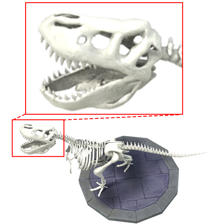
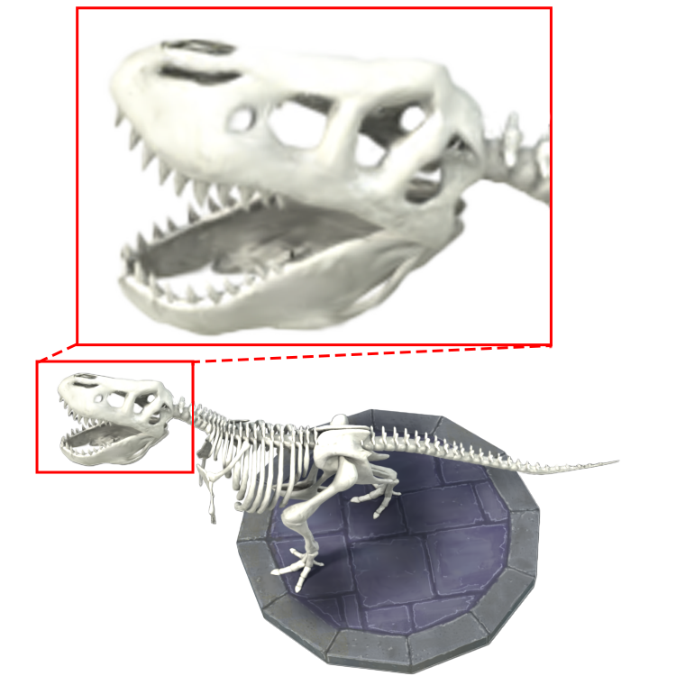
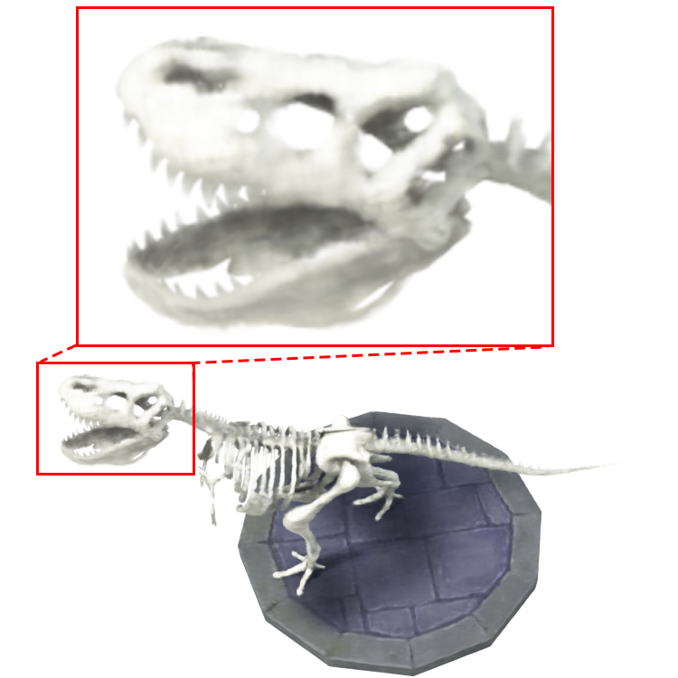
StandUp
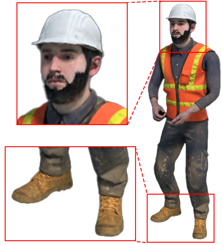
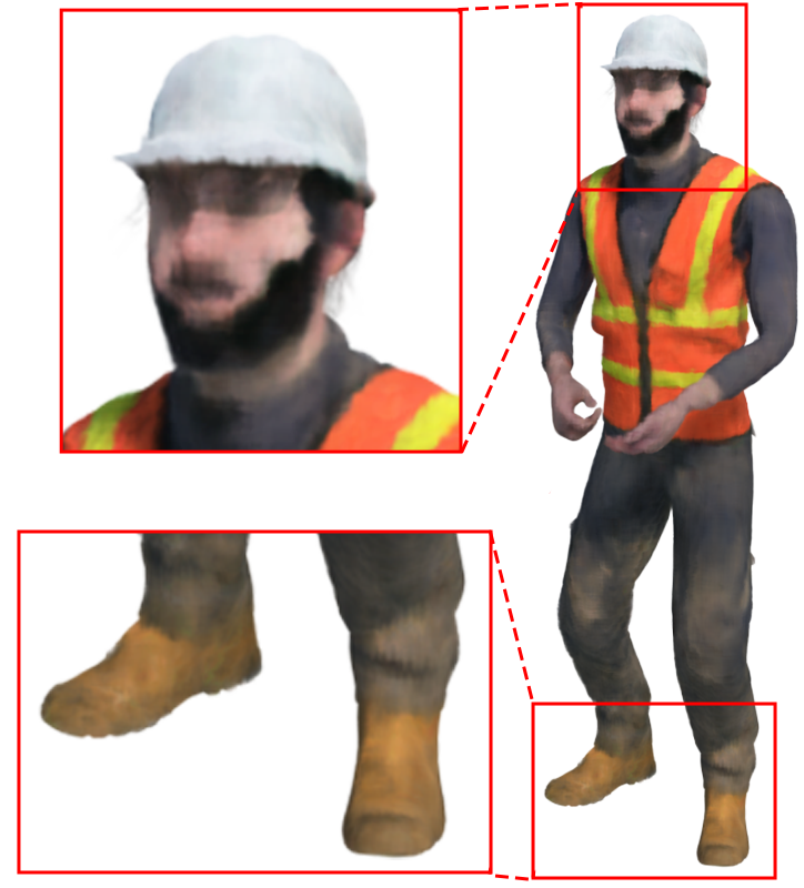
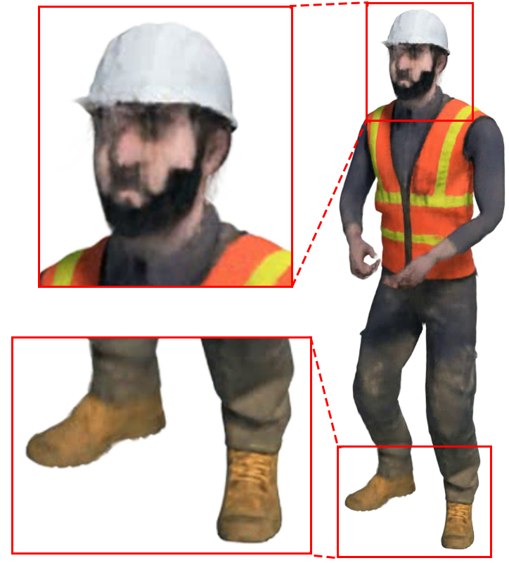
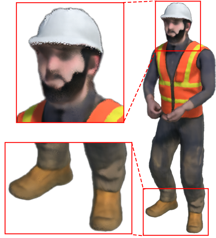
Mutant
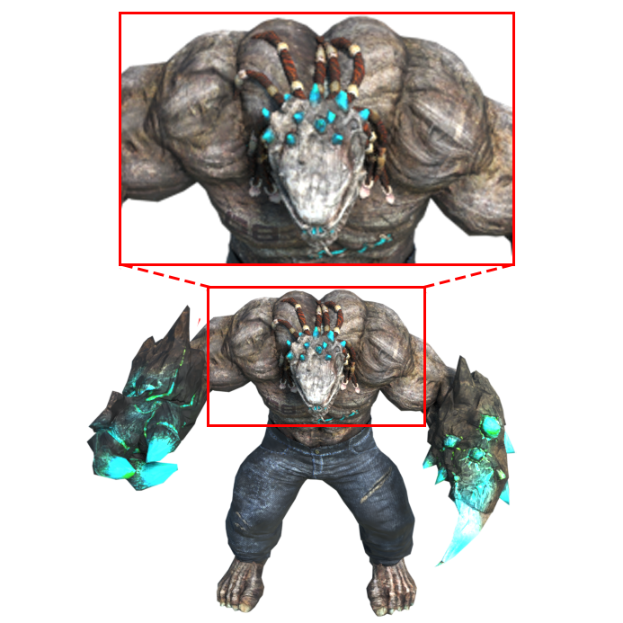
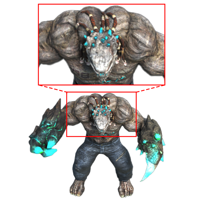
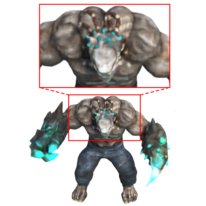
Lego
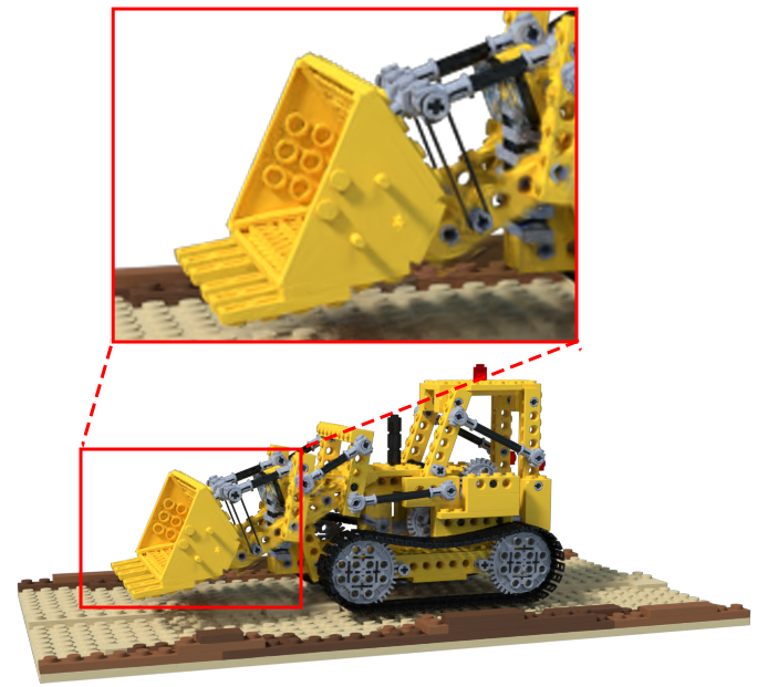
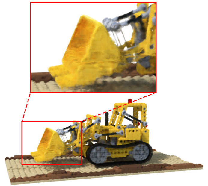
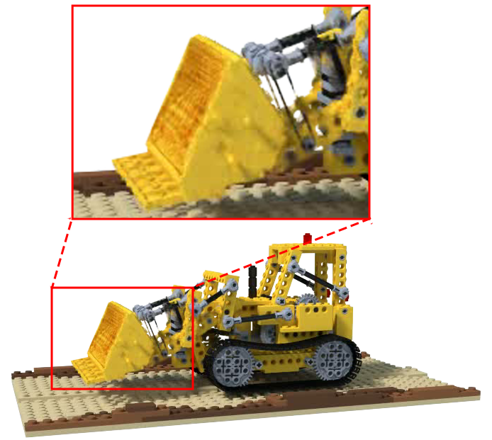
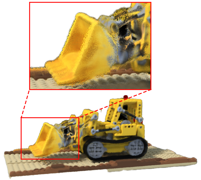
Jumpingjacks
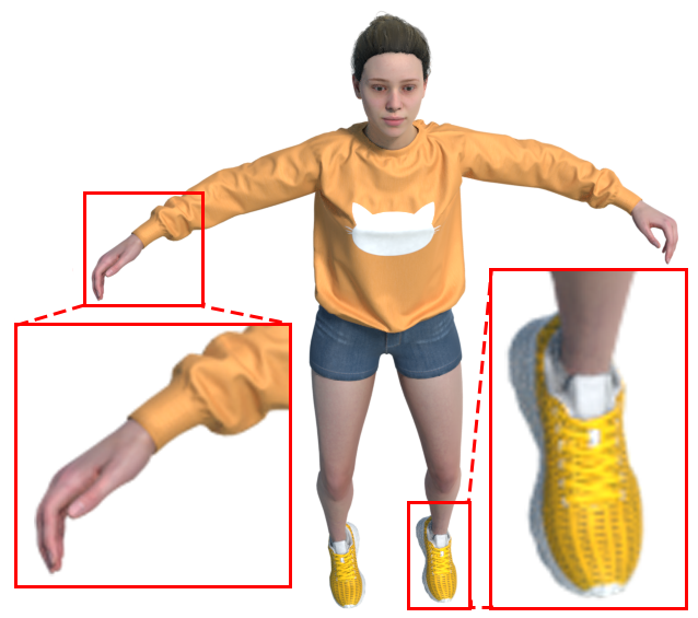
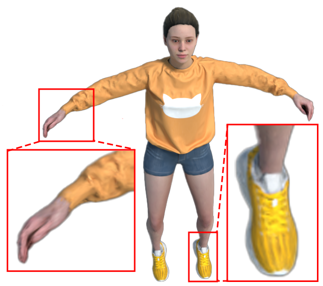
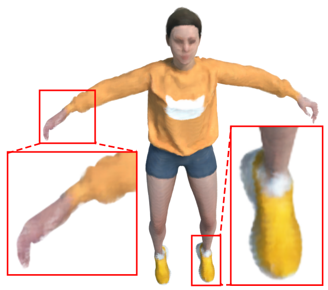
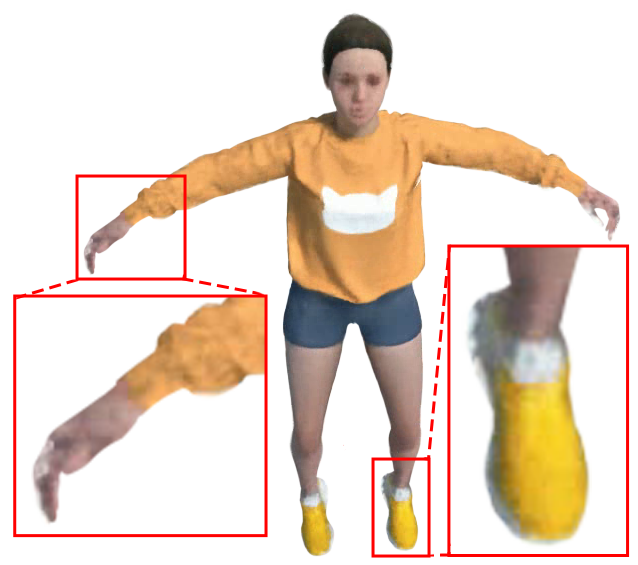
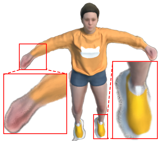
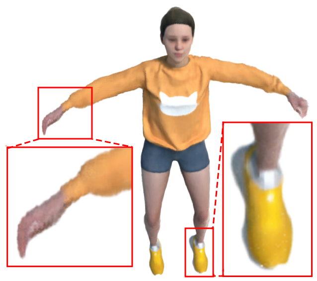
hook
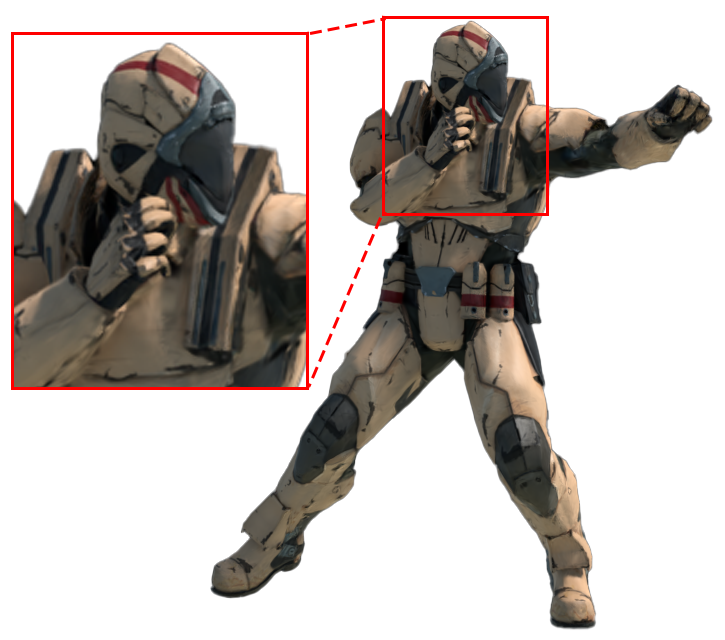
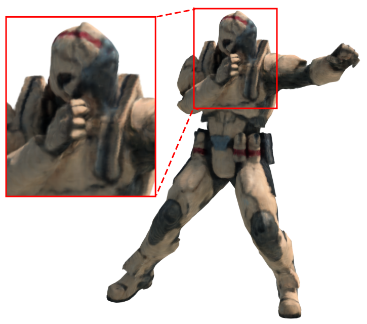
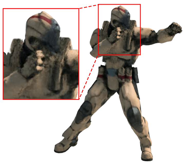
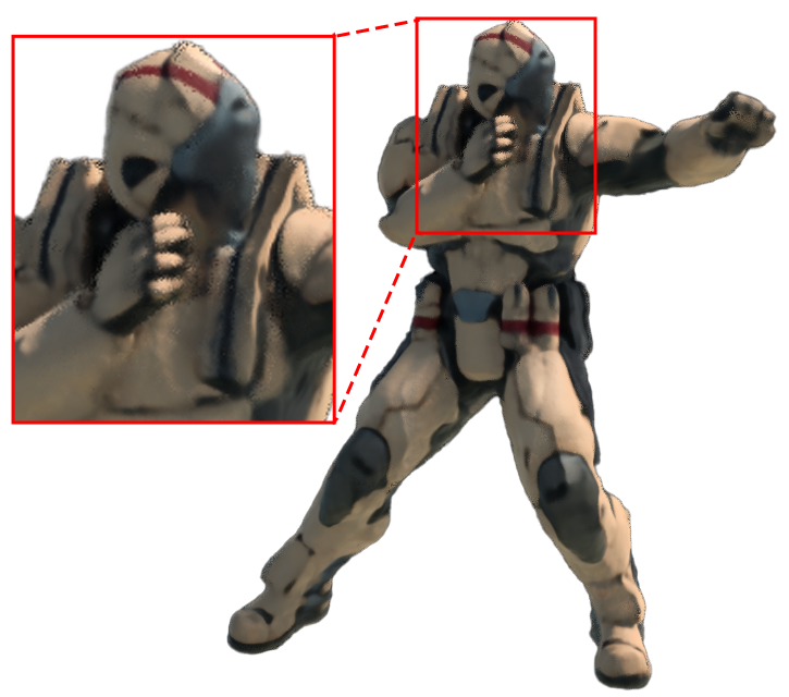
HellWarrior
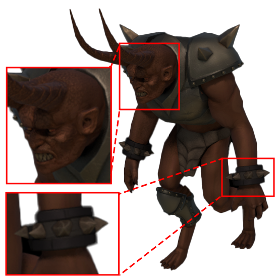
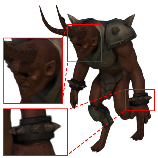
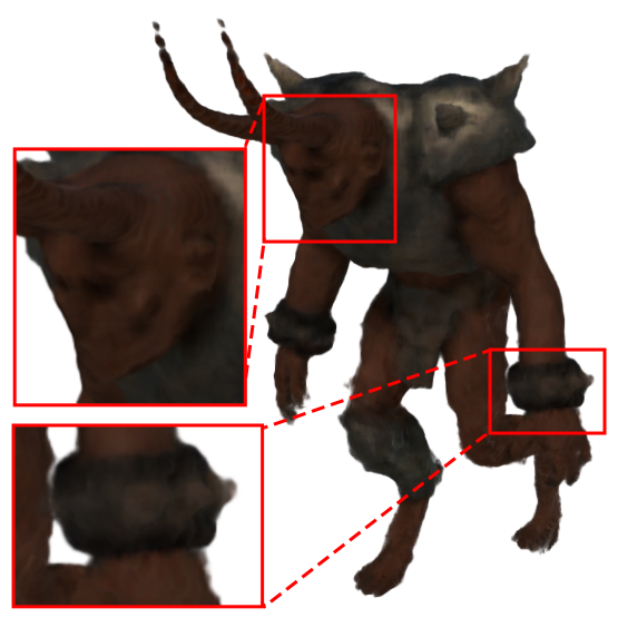
BouncingBalls

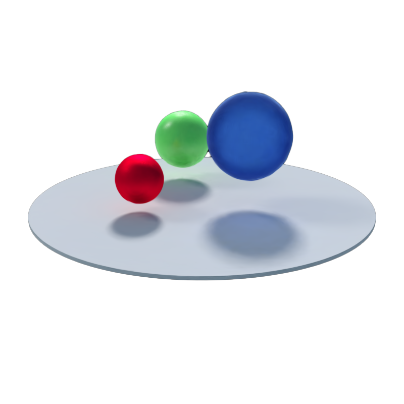
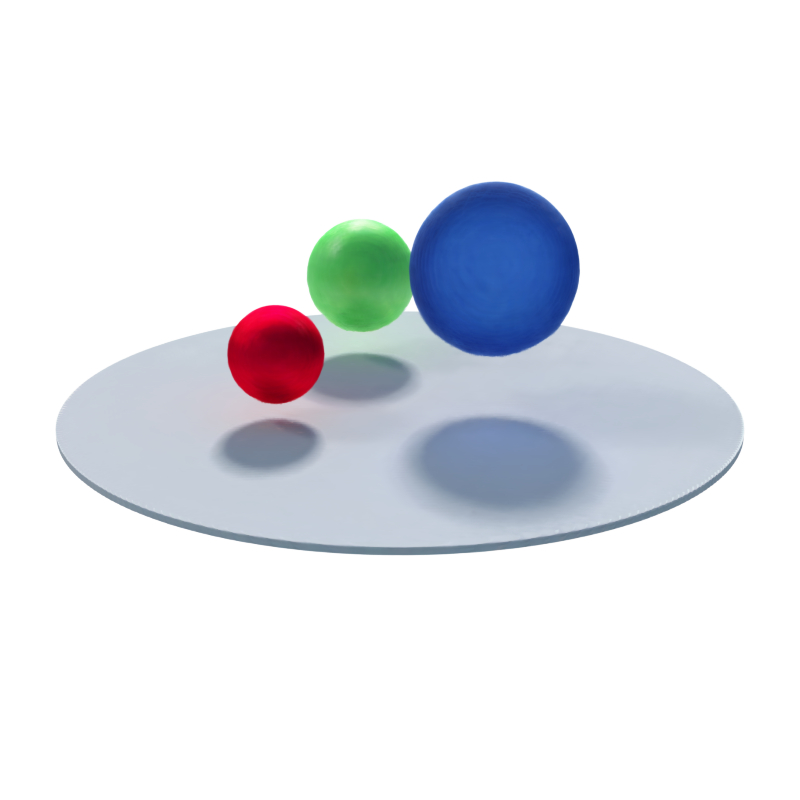
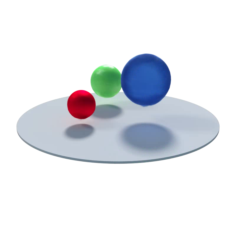
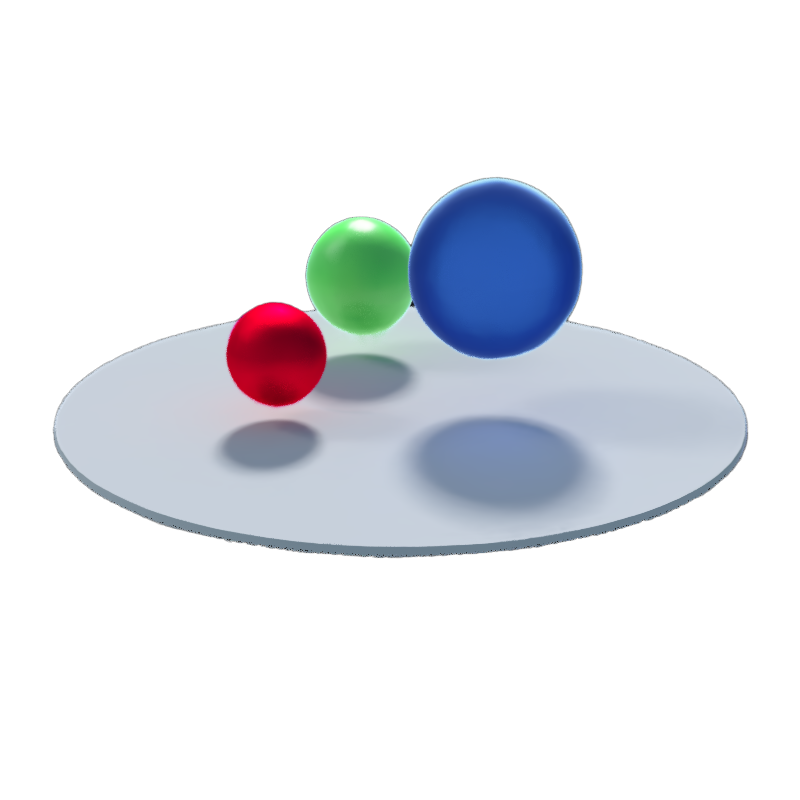
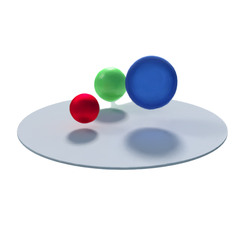
Figure 3: Qualitative comparisons of baselines and our method on monocular synthetic dataset. We visualize each scene using baselines and our method. Experimental results indicate that our approach recovers more details when rendering novel viewpoints and can reconstruct more delicate structures over time, such as hands or skeletons. The efficacy of Deformable-GS can be attributed to its capability to equally back-propagate the gradient to both the Deformation Field and the 3D Gaussians. Larger gradients in the dynamic portion of the Deformation Field can further assist the 3D Gaussians in achieving better densification in dynamic regions.

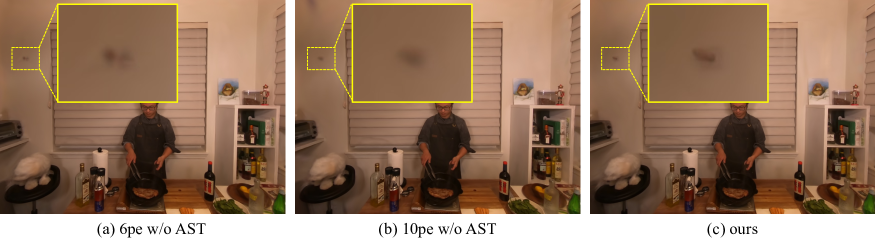
Figure 4: Ablation study. We conduct ablation studies focusing on the annealing smooth training scheme within real-world datasets, wherein pe signifies the positional encoding over time. Compared with the reduced order (a) and the original order (b) of positional encoding over time, it becomes evident that the annealing smooth training strategy (c) effectively preserves high-frequency information. Simultaneously, it mitigates the temporal overfitting challenges instigated by imprecise pose estimations.

	GT	Ours	TiNeuVox	HyperNeRF	NeRF-DS	3D-GS
as
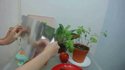
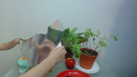
bell
sieve

Figure 5: Qualitative comparisons of baselines and our method on NeRF-DS real-world dataset. Experimental results indicate that our method can achieve superior rendering quality on real-world datasets where the pose is not absolutely precise.

4 Experiment

In this section, we present the experimental evaluation of our method. To give proof of effectiveness, we evaluate our approach on the benchmark which consists of the synthetic dataset from D-NeRF [34] and real-world datasets sourced from HyperNeRF [31] and NeRF-DS [50]. The division on training and testing part, as well as the image resolution, aligns perfectly with the original paper.

4.1 Implementation Details

We implement our framework using PyTorch [32] and modify the differentiable Gaussian rasterization by incorporating depth visualization. For training, we conducted training for a total of 40k iterations. During the initial 3k iterations, we solely trained the 3D Gaussians to attain relatively stable positions and shapes. Subsequently, we jointly train the 3D Gaussians and the deformation field. For optimization, a single Adam optimizer [17] is used but with a different learning rate for each component: the learning rate of 3D Gaussians is exactly the same as the official implementation, while the learning rate of the deformation network undergoes exponential decay, ranging from 8e-4 to 1.6e-6. Adam’s $\beta$ value range is set to (0.9, 0.999). Experiments with synthetic datasets were all conducted against a black background and at a full resolution of 800x800. All the experiments were done on an NVIDIA RTX 3090.

4.2 Results and Comparisons

Comparisons on synthetic dataset.

In our experiments, we benchmarked our method against several baselines using the monocular synthetic dataset introduced by D-NeRF [34]. The quantitative evaluation, presented in Tab. 1, offers compelling evidence of the superior performance of our approach over the current state-of-the-art. Notably, metrics pertinent to structural consistency, such as LPIPS and SSIM, demonstrate our method’s pronounced superiority.

For a more visual assessment, we provide qualitative results in Fig. 3. These visual comparisons underscore the capability of our method in delivering high-fidelity dynamic scene modeling. It’s evident from the results that our approach ensures enhanced consistency and captures intricate rendering details in novel-view renderings.

Comparisons on real-world dataset.

We compare our method with the baselines using the monocular real-world dataset from NeRF-DS [50] and HyperNeRF [31]. It should be noted that the camera poses for some of the HyperNeRF datasets are very inaccurate. Given that metrics like PSNR, designed to assess image rendering quality, are inclined to penalize slight deviations more than blurring, we have refrained from incorporating HyperNeRF in our quantitative analysis. For a qualitative analysis of HyperNeRF, please refer to the supplementary materials. The quantitative and qualitative evaluations for the NeRF-DS dataset are detailed in Tab. 2 and Fig. 5, respectively. These results attest to the robustness of our method when applied to real-world scenes, even when the associated poses are not perfectly accurate.

Rendering Efficiency.

The rendering speed is correlated with the quantity of 3D Gaussians. Overall, when the number of 3D Gaussians is below 250k, our method can achieve real-time rendering over 30 FPS on an NVIDIA RTX 3090. Detailed results can be found in the supplementary material.

Depth Visualization.

We visualized the depth of synthetic dataset scenes in Fig. 6 to demonstrate that our deformation network is well fitted to produce temporal transformation rather than relying on color-based hard-coding. The precise depth underscores the accuracy of our geometric reconstruction, proving highly advantageous for the novel-view synthesis task.

4.3 Ablation Study

Annealing smooth training.

As illustrated in Fig. 4 and Tab. 2, this mechanism fosters improved convergence towards intricate regions, effectively mitigating the overfitting tendencies in real-world datasets. Furthermore, it is unequivocally clear from our observations that this strategy significantly bolsters the temporal smoothness of the deformation field. See more ablations in supplementary materials.

5 Limitations

Through our experimental evaluations, we observed that the convergence of 3D Gaussians is profoundly influenced by the diversity of perspectives. As a result, datasets characterized by sparse viewpoints and limited viewpoint coverage may lead our method to encounter overfitting challenges. Additionally, the efficacy of our approach is contingent upon the accuracy of pose estimations. This dependency was evident when our method did not achieve optimal PSNR values on the Nerfies/HyperNeRF dataset, attributable to deviations in pose estimation via COLMAP. Furthermore, the temporal complexity of our approach is directly proportional to the quantity of 3D Gaussians. In scenarios with an extensive array of 3D Gaussians, there is a potential escalation in both training duration and memory consumption. Lastly, our evaluations have predominantly revolved around scenes with moderate motion dynamics. The method’s adeptness at handling intricate human motions, such as nuanced facial expressions, remains an open question. We perceive these constraints as promising directions for subsequent research endeavors.

	PSNR $\uparrow$	SSIM $\uparrow$	LPIPS $\downarrow$
3D-GS	20.29	0.7816	0.2920
TiNeuVox	21.61	0.8234	0.2766
HyperNeRF	23.45	0.8488	0.1990
NeRF-DS	23.60	0.8494	0.1816
Ours (w/o AST)	23.97	0.8346	0.2037
Ours	24.11	0.8525	0.1769

Table 2: Metrics on NeRF-DS dataset. We computed the mean of the metrics across all seven scenes. Cells are highlighted as follows: best, second best, and third best. For individual metrics about each scene, please refer to the supplementary material.

Figure 6: Depth Visualization. We visualized the depth map of the D-NeRF dataset. The first row includes bouncing-balls, hell-warrior, hook, and jumping-jacks, while the second row includes lego, mutant, standup, and trex.

6 Conclusions

We introduce a novel deformable 3D Gaussian splatting method, specifically designed for monocular dynamic scene modeling, which surpasses existing methods in both quality and speed. By learning the 3D Gaussians in canonical space, we enhance the versatility of the 3D-GS differentiable rendering pipeline for dynamically captured monocular scenes. It’s crucial to recognize that point-based methods, in comparison to implicit representations, are more editable and better suited for post-production tasks. Additionally, our method incorporates an annealing smooth training strategy, aimed at reducing overfitting associated with time encoding while maintaining intricate scene details, without adding any extra training overhead. Experimental results demonstrate that our method not only achieves superior rendering effects but is also capable of real-time rendering.

Appendix A Overview

The appendix provides some implementation details and further results that accompany the paper.

• Section B introduces the implementation details of the network architecture in our approach.

• Section C provides additional results, including more visualizations, rendering efficiency, more comparisons, and more ablations.

• Section D discusses the failure cases of our method.

Appendix B Implementation Details

B.1 Network Architecture of the Deformation Field

We learn the deformation field with an MLP network $\mathcal{F_{\theta}}:(\gamma(\mathbf{x}),\gamma(t))\rightarrow(\delta x,\delta r,\delta s)$, which maps from each coordinate of 3D Gaussians and time to their corresponding deviations in position, rotation, and scaling. The weights $\theta$ of the MLP are optimized through this mapping. As shown in Fig. 7, our MLP $\mathcal{F_{\theta}}$ initially processes the input through eight fully connected layers that employ ReLU activations and feature 256-dimensional hidden layers, and outputs a 256-dimensional feature vector. This vector is subsequently passed through three additional fully connected layers (without activation) to separately output the offsets over time for position, rotation, and scaling. It should be noted that similar to NeRF, we concatenate the feature vector and the input in the fourth layer. Due to the compact structure of MLP, our additional storage compared to 3D Gaussians is only 2MB.

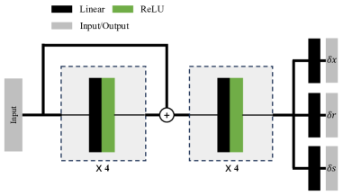
Figure 7: The architecture of our deformation MLP.

broom
	train	train-depth	test	test-depth

Figure 8: Failure case on inaccurate pose. Excessively inaccurate poses can lead to the failure of the convergence on the training set.

Method	Sieve			Plate			Bell			Press
	PSNR$\uparrow$	SSIM$\uparrow$	LPIPS$\downarrow$	PSNR$\uparrow$	SSIM$\uparrow$	LPIPS$\downarrow$	PSNR$\uparrow$	SSIM$\uparrow$	LPIPS$\downarrow$	PSNR$\uparrow$	SSIM $\uparrow$	LPIPS$\downarrow$
3D-GS	23.16	0.8203	0.2247	16.14	0.6970	0.4093	21.01	0.7885	0.2503	22.89	0.8163	0.2904
TiNeuVox	21.49	0.8265	0.3176	20.58	0.8027	0.3317	23.08	0.8242	0.2568	24.47	0.8613	0.3001
HyperNeRF	25.43	0.8798	0.1645	18.93	0.7709	0.2940	23.06	0.8097	0.2052	26.15	0.8897	0.1959
NeRF-DS	25.78	0.8900	0.1472	20.54	0.8042	0.1996	23.19	0.8212	0.1867	25.72	0.8618	0.2047
Ours (w/o AST)	25.33	0.8620	0.1594	20.32	0.7173	0.3914	25.62	0.8498	0.1540	25.78	0.8613	0.1919
Ours	25.70	0.8715	0.1504	20.48	0.8124	0.2224	25.74	0.8503	0.1537	26.01	0.8646	0.1905
	Cup			As			Basin			Mean
Method	PSNR$\uparrow$	SSIM$\uparrow$	LPIPS$\downarrow$	PSNR$\uparrow$	SSIM$\uparrow$	LPIPS$\downarrow$	PSNR$\uparrow$	SSIM$\uparrow$	LPIPS$\downarrow$	PSNR$\uparrow$	SSIM $\uparrow$	LPIPS$\downarrow$
3D-GS	21.71	0.8304	0.2548	22.69	0.8017	0.2994	18.42	0.7170	0.3153	20.29	0.7816	0.2920
TiNeuVox	19.71	0.8109	0.3643	21.26	0.8289	0.3967	20.66	0.8145	0.2690	21.61	0.8234	0.2766
HyperNeRF	24.59	0.8770	0.1650	25.58	0.8949	0.1777	20.41	0.8199	0.1911	23.45	0.8488	0.1990
NeRF-DS	24.91	0.8741	0.1737	25.13	0.8778	0.1741	19.96	0.8166	0.1855	23.60	0.8494	0.1816
Ours (w/o AST)	24.80	0.8848	0.1571	26.29	0.8800	0.1830	19.68	0.7869	0.1888	23.97	0.8346	0.2037
Ours	24.86	0.8908	0.1532	26.31	0.8842	0.1783	19.67	0.7934	0.1901	24.11	0.8524	0.1769

Table 3: Quantitative comparison on NeRF-DS dataset per-scene. We color each cell as best, second best, and third best. Our method, overall, achieves the best rendering quality and robust convergence in the majority of scenes. It is worth noting that the metrics we used are the same as those in the main text, with LPIPS using the VGG network. The slight differences in our measurement metrics, compared to those used in NeRF-DS and HyperNeRF, are due to their papers employing MS-SSIM and LPIPS with the AlexNet.

D-NeRF Dataset			NeRF-DS Dataset			HyperNeRF Dataset
Scene	FPS	Num (k)	Scene	FPS	Num (k)	Scene	FPS	Num (k)
Lego	24	300	AS	48	185	Espresso	15	620
Jump	85	90	Basin	29	250	Americano	6	1300
Bouncing	38	170	Bell	18	400	Cookie	9	1080
T-Rex	30	220	Cup	35	200	Chicken	10	740
Mutant	40	170	Plate	31	230	Torchocolate	8	1030
Warrior	172	40	Press	48	185	Lemon	23	420
Standup	93	80	Sieve	35	200	Hand	6	1750
Hook	45	150				Printer	12	650

Table 4: Experiments on FPS with respect to the number of 3D Gaussians. The results of the experiments demonstrate that our method is capable of real-time rendering on a 3090 GPU when the number of point clouds is less than 250k. The excessively high number of 3D Gaussians in HyperNeRF reflects the critical importance of the camera pose accuracy for the convergence of our method.

	GT	Ours	Tineuvox	HyperNeRF	3D-GS
torchocolate
hand
lemon
printer
chicken

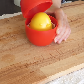
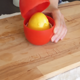
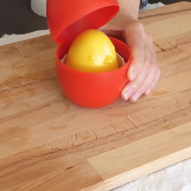
Figure 9: Qualitative comparisons of baselines and our method on HyperNeRF dataset. The first three rows present the results of the time interpolation task, while the last two rows depict the outcomes of the novel viewpoint synthesis task. Experimental results indicate that our method can achieve superior rendering quality on real datasets where the pose is not absolutely precise.

kuka
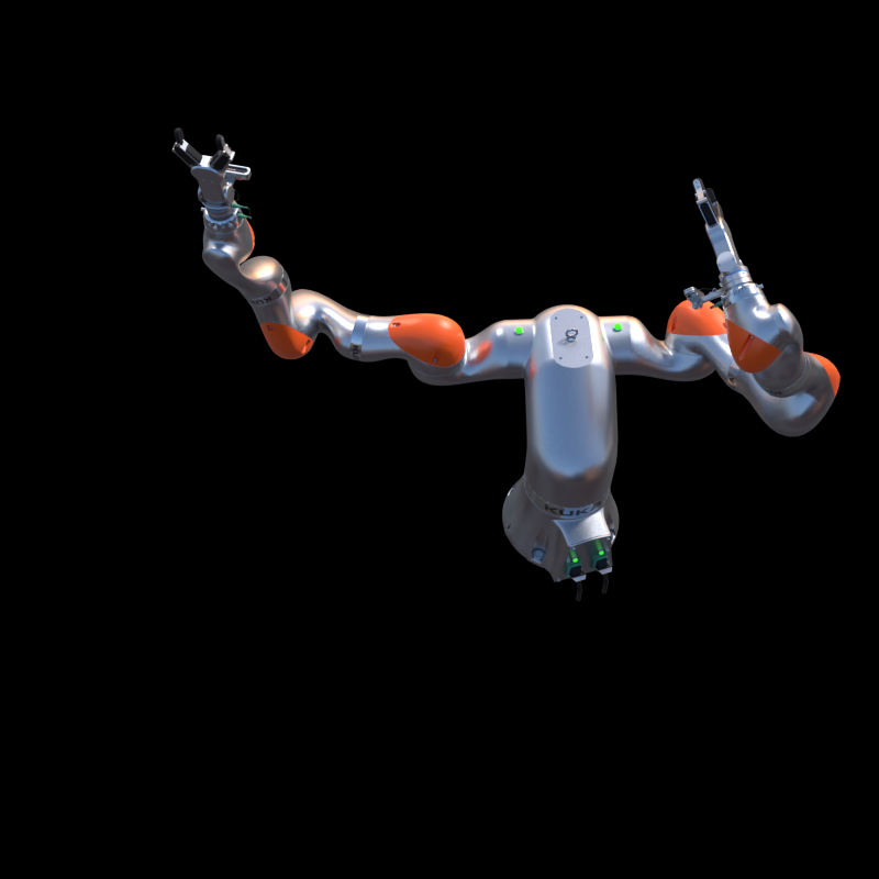
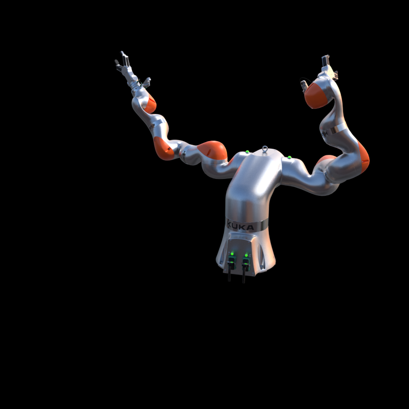
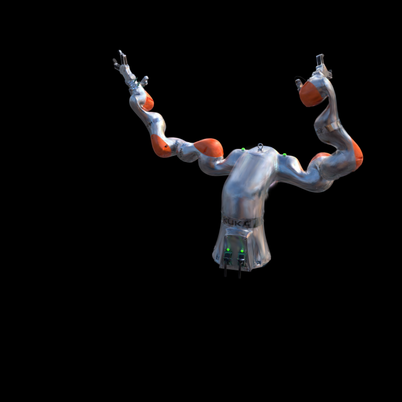
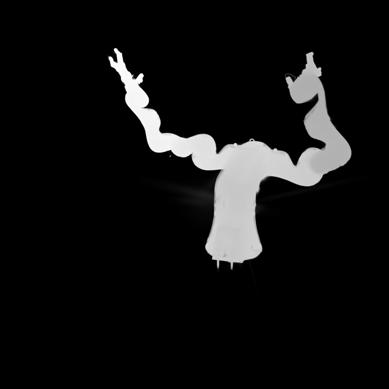
robot
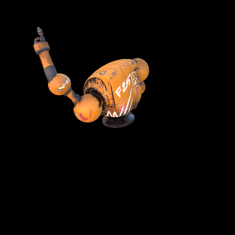
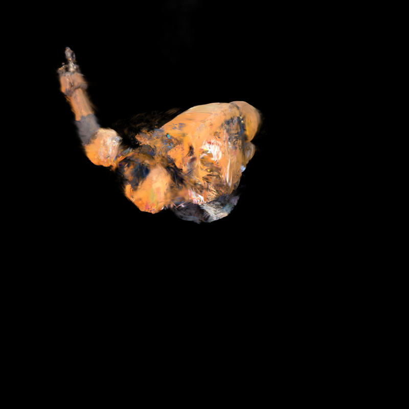
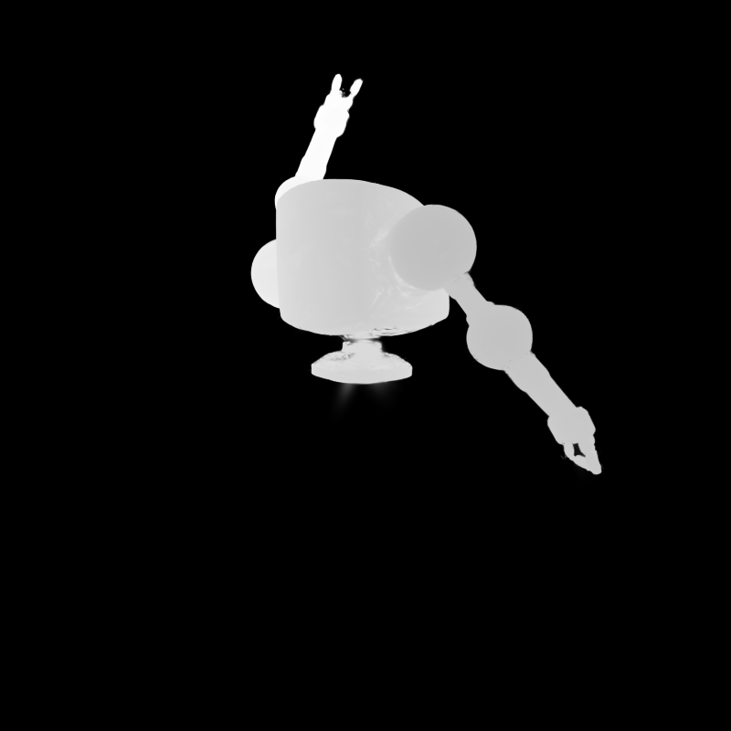
glove
	gt	render	depth	gt-swap	render-swap	depth-swap

Figure 10: Failure case on few training viewpoints. The first three columns represent the original dataset configurations. The term swap indicates the exchange of training and test sets, thereby ensuring that the model’s inputs possess a sufficiently diverse array of viewpoints

	lego	jump	boungcing	trex	mutant	warrior	standup	hook	mean
ours	33.07	37.72	41.01	38.10	42.63	41.54	44.62	37.42	39.51
ours-SE(3)	32.91	37.60	41.05	38.29	42.83	41.73	44.68	37.60	39.58

Table 5: Comparison with SE(3) deformation field on the D-NeRF dataset.

	as	basin	bell	cup	plate	press	sieve	mean
ours	26.31	19.67	25.74	24.86	20.48	26.01	25.70	24.11
ours-SE(3)	26.37	19.64	25.43	24.83	20.28	25.63	25.46	23.95

Table 6: Comparison with SE(3) deformation field on the NeRF-DS dataset.

	Hell Warrior			Mutant			Hook
	PSNR$\uparrow$	SSIM$\uparrow$	LPIPS$\downarrow$	PSNR$\uparrow$	SSIM$\uparrow$	LPIPS$\downarrow$	PSNR$\uparrow$	SSIM$\uparrow$	LPIPS$\downarrow$
w/o $\delta s$	41.55	0.9878	0.0223	42.15	0.9949	0.0053	37.01	0.9859	0.0153
w/o $\delta r$	41.17	0.9866	0.0256	42.51	0.9950	0.0054	36.82	0.9852	0.0167
w r&s	40.39	0.9833	0.0323	41.30	0.9934	0.0075	36.15	0.9818	0.0214
ours	41.54	0.9873	0.0234	42.63	0.9951	0.0052	37.42	0.9867	0.0144
	Bouncing Balls			Lego			T-Rex
	PSNR$\uparrow$	SSIM$\uparrow$	LPIPS$\downarrow$	PSNR$\uparrow$	SSIM$\uparrow$	LPIPS$\downarrow$	PSNR$\uparrow$	SSIM$\uparrow$	LPIPS$\downarrow$
w/o $\delta s$	40.82	0.9952	0.0095	31.30	0.9705	0.0260	37.39	0.9928	0.0105
w/o $\delta r$	41.11	0.9953	0.0092	32.87	0.9783	0.0192	37.99	0.9931	0.0101
w r&s	39.89	0.9945	0.0117	33.71	0.9798	0.0181	37.06	0.9923	0.0113
ours	41.01	0.9953	0.0093	33.07	0.9794	0.0183	38.10	0.9933	0.0098
	Stand Up			Jumping Jacks			Mean
	PSNR$\uparrow$	SSIM$\uparrow$	LPIPS$\downarrow$	PSNR$\uparrow$	SSIM$\uparrow$	LPIPS$\downarrow$	PSNR$\uparrow$	SSIM$\uparrow$	LPIPS$\downarrow$
w/o $\delta s$	44.05	0.9946	0.0074	37.49	0.9895	0.0129	38.97	0.9889	0.0137
w/o $\delta r$	44.18	0.9946	0.0075	37.48	0.9893	0.0138	39.27	0.9897	0.0134
w r&s	42.88	0.9932	0.0097	37.00	0.9878	0.0164	38.55	0.9883	0.0160
ours	44.62	0.9951	0.0063	37.72	0.9897	0.0126	39.51	0.9902	0.0124

Table 7: Ablations on network architecture. We color each cell as best and second best. $\delta r$ and $\delta s$ denote the output components of the MLP model. The term w r&s signifies that the model inputs include not only time and the position of the 3D Gaussians but also the 3D Gaussians’ rotation and scaling. The experimental outcomes affirm that our network architecture is the most advantageous.

	lego	jump	bouncing	trex	mutant	warrior	standup	hook	mean
ours	33.07	37.72	41.01	38.10	42.63	41.54	44.62	37.42	39.51
ours-white	32.03	36.87	43.52	38.57	42.11	32.75	42.40	36.60	38.10
ours-best	33.07	37.72	43.52	38.57	42.63	41.54	44.62	37.42	39.89

Table 8: Comparison with different background colors on the D-NeRF dataset.We explored the impact of different background colors on rendering metrics using the D-NeRF dataset. The experimental results showed that overall, a black background yielded higher metrics, while bouncing and trex scenes performed better with a white background, and the warrior scene had higher metrics with a black background. To ensure experimental consistency, we uniformly used a black background in the main text. If one wishes to pursue the best metrics for a specific scene, one can refer to this table to adjust the background color.

Our deformation field does not employ any grid/plane-based structures which have been demonstrated to be superior in static scenes because these structures are predicated on a low-rank tensor assumption [7]. Dynamic scenes possess a higher rank compared to static scenes, and explicit point-based rendering exacerbates the rank of the scene.

B.2 Optimization Loss

During the training of our deformable Gaussians, we deform the 3D Gaussians at each timestep into the canonical space. We then optimize both the deformation network and the 3D Gaussians using a combination of $\mathcal{L}_{1}$ loss and D-SSIM loss [15]:

$$\mathcal{L}=(1-\lambda)\mathcal{L}_{1}+\lambda\mathcal{L}_{\text{D-SSIM}},$$ (7)

where $\lambda=0.2$ is used in all our experiments.

Appendix C Additional Results

C.1 Per-Scene Results on the NeRF-DS Dataset

In Tab. 3, we provide the results for individual scenes associated with Sec. 4 of the main paper. It can be observed that our method achieved superior metrics in almost every scene compared to those without AST, underscoring the generalizability of AST on real datasets where the pose is not perfectly accurate. Overall, our method outperforms baselines on the NeRF-DS Dataset.

C.2 Results on the HyperNeRF Dataset

We visualize the results of the HyperNeRF dataset in Fig. 9. Notably, metrics designed to assess image rendering quality, such as PSNR, tend to penalize minor offsets more heavily than blurring. Therefore, for datasets with less accurate camera poses, like HyperNeRF, our method’s quantitative metrics might not consistently outperform those of methods yielding blurred outputs when faced with imprecise camera poses. Despite this, our rendered images often exhibit fewer artifacts and greater clarity. This phenomenon aligns with observations reported in Nerfies [30] and HyperNeRF [31].

C.3 Results on Rendering Efficiency

In our research, we present comprehensive Frames Per Second (FPS) testing results in Tab. 4. Tests were conducted on one NVIDIA RTX 3090. It is observed that when the number of point clouds remains below $\sim$250k, our method can achieve real-time rendering at rates greater than 30 FPS. A point of note is that the point cloud count reconstructed from the HyperNeRF dataset significantly exceeds that of other datasets, reaching a level of 1,000k. This excessive count is attributed to the highly inaccurate camera poses within the HyperNeRF dataset. In contrast, the NeRF-DS dataset, while also being derived from the real world, exhibits more accurate poses, resulting in a reconstructed point cloud count within a reasonable range. This issue of an overabundant point cloud count occurs not only in scenes with inaccurate poses but also in those with sparse viewpoints, as evidenced in scenes like the D-NeRF’s Lego scene, which was trained on merely 50 images.

C.4 More Ablations

Network architecture.

We present ablation experiments on the architecture of our purely implicit network, as shown in Tab. 7. The results of these experiments suggest that the structure within our pipeline is optimal. Notably, we did not adopt Grid/Plane-based structures because dynamic scenes do not conform to the low-rank assumption. Furthermore, the explicit point-based rendering of 3D-GS exacerbates the rank of dynamic scenes. Our early experimental validations have corroborated this assertion.

C.5 Background color

In the research of Neural Rendering, it’s common to use a black or white background for rendering scenes without a background. In our experiments, we found that the background color has an impact on certain scenes in the D-NeRF dataset. The experimental results are shown in Tab. 8. Overall, a black background yields better rendering results. For the sake of consistency in our experiments, we uniformly used a black background in our main text experiments. However, for the bouncing and trex scenes, using a white background can produce better results.

C.6 Deformation using SE(3) Field

Drawing inspiration from Nerfies [30], we applied a 6-DOF SE(3) field that accounts for rotation to the transformation of 3D Gaussian positions. The experimental results, presented in Tab. 5 and Tab. 6, indicate that this constraint offers a minor improvement on the D-NeRF dataset. However, it appears to diminish the quality on the more complex real-world NeRF-DS dataset. Moreover, the additional computational overhead introduced by the SE(3) Field approximately increases 50 % of the training time and results in about a 20% decrease in FPS during rendering. Consequently, we opted to utilize a direct addition without imposing SE(3) constraints on the transformation of position.

Appendix D Failure Cases

Inaccurate poses.

In our research, we find that inaccurate poses can lead to the failure of the convergence of deformable-gs, as illustrated in Fig. 8. For implicit representations, their inherent smoothness can maintain robustness in the face of minor deviations in pose. However, for the explicit point-based rendering, such inaccuracies are particularly detrimental, resulting in inconsistencies in the scene at different moments.

Few training viewpoints.

In our study, a notable scarcity of training views presents a dual challenge: both few-shot learning and a limited number of viewpoints. Either aspect can lead to overfitting in deformable-gs and even in 3D-GS on the training set. As demonstrated in Fig. 10, significant overfitting is evident in the DeVRF [23] dataset. The training set for this scene contains 100 images, but the viewpoints for training are limited to only four. However, by swapping the training and test sets, where the test set contained an equal number of 100 images and viewpoints, we obtained markedly better results.

References

- [1] Benjamin Attal, Eliot Laidlaw, Aaron Gokaslan, Changil Kim, Christian Richardt, James Tompkin, and Matthew O’Toole. Törf: Time-of-flight radiance fields for dynamic scene view synthesis. Advances in Neural Information Processing Systems, 34:26289–26301, 2021.
- [2] Jonathan T. Barron, Ben Mildenhall, Matthew Tancik, Peter Hedman, Ricardo Martin-Brualla, and Pratul P. Srinivasan. Mip-nerf: A multiscale representation for anti-aliasing neural radiance fields. ICCV, 2021.
- [3] Jonathan T. Barron, Ben Mildenhall, Dor Verbin, Pratul P. Srinivasan, and Peter Hedman. Mip-nerf 360: Unbounded anti-aliased neural radiance fields. CVPR, 2022.
- [4] Jonathan T. Barron, Ben Mildenhall, Dor Verbin, Pratul P. Srinivasan, and Peter Hedman. Zip-nerf: Anti-aliased grid-based neural radiance fields. ICCV, 2023.
- [5] Mark Boss, Raphael Braun, Varun Jampani, Jonathan T. Barron, Ce Liu, and Hendrik P.A. Lensch. Nerd: Neural reflectance decomposition from image collections. In IEEE International Conference on Computer Vision (ICCV), 2021.
- [6] Ang Cao and Justin Johnson. Hexplane: A fast representation for dynamic scenes. CVPR, 2023.
- [7] Anpei Chen, Zexiang Xu, Andreas Geiger, Jingyi Yu, and Hao Su. Tensorf: Tensorial radiance fields. In European Conference on Computer Vision (ECCV), 2022.
- [8] Zhiqin Chen, Thomas Funkhouser, Peter Hedman, and Andrea Tagliasacchi. Mobilenerf: Exploiting the polygon rasterization pipeline for efficient neural field rendering on mobile architectures. In Proceedings of the IEEE/CVF Conference on Computer Vision and Pattern Recognition, pages 16569–16578, 2023.
- [9] Alvaro Collet, Ming Chuang, Pat Sweeney, Don Gillett, Dennis Evseev, David Calabrese, Hugues Hoppe, Adam Kirk, and Steve Sullivan. High-quality streamable free-viewpoint video. ACM Transactions on Graphics (ToG), 34(4):1–13, 2015.
- [10] Kangle Deng, Andrew Liu, Jun-Yan Zhu, and Deva Ramanan. Depth-supervised NeRF: Fewer views and faster training for free. In Proceedings of the IEEE/CVF Conference on Computer Vision and Pattern Recognition (CVPR), June 2022.
- [11] Jiemin Fang, Taoran Yi, Xinggang Wang, Lingxi Xie, Xiaopeng Zhang, Wenyu Liu, Matthias Nießner, and Qi Tian. Fast dynamic radiance fields with time-aware neural voxels. In SIGGRAPH Asia 2022 Conference Papers, 2022.
- [12] Stephan J Garbin, Marek Kowalski, Matthew Johnson, Jamie Shotton, and Julien Valentin. Fastnerf: High-fidelity neural rendering at 200fps. In Proceedings of the IEEE/CVF International Conference on Computer Vision, pages 14346–14355, 2021.
- [13] Peter Hedman, Pratul P Srinivasan, Ben Mildenhall, Jonathan T Barron, and Paul Debevec. Baking neural radiance fields for real-time view synthesis. In Proceedings of the IEEE/CVF International Conference on Computer Vision, pages 5875–5884, 2021.
- [14] Takeo Kanade, Peter Rander, and PJ Narayanan. Virtualized reality: Constructing virtual worlds from real scenes. IEEE Multimedia, 4(1):34–47, 1997.
- [15] Bernhard Kerbl, Georgios Kopanas, Thomas Leimkühler, and George Drettakis. 3d gaussian splatting for real-time radiance field rendering. ACM Transactions on Graphics, 42(4), July 2023.
- [16] Leonid Keselman and Martial Hebert. Approximate differentiable rendering with algebraic surfaces. In European Conference on Computer Vision (ECCV), 2022.
- [17] Diederik Kingma and Jimmy Ba. Adam: A method for stochastic optimization. In International Conference on Learning Representations (ICLR), 2015.
- [18] Hao Li, Linjie Luo, Daniel Vlasic, Pieter Peers, Jovan Popović, Mark Pauly, and Szymon Rusinkiewicz. Temporally coherent completion of dynamic shapes. ACM Transactions on Graphics (TOG), 31(1):1–11, 2012.
- [19] Tianye Li, Mira Slavcheva, Michael Zollhoefer, Simon Green, Christoph Lassner, Changil Kim, Tanner Schmidt, Steven Lovegrove, Michael Goesele, Richard Newcombe, et al. Neural 3d video synthesis from multi-view video. In Proceedings of the IEEE/CVF Conference on Computer Vision and Pattern Recognition, pages 5521–5531, 2022.
- [20] Zhaoshuo Li, Thomas Müller, Alex Evans, Russell H Taylor, Mathias Unberath, Ming-Yu Liu, and Chen-Hsuan Lin. Neuralangelo: High-fidelity neural surface reconstruction. In IEEE Conference on Computer Vision and Pattern Recognition (CVPR), 2023.
- [21] Chen-Hsuan Lin, Wei-Chiu Ma, Antonio Torralba, and Simon Lucey. Barf: Bundle-adjusting neural radiance fields. In IEEE International Conference on Computer Vision (ICCV), 2021.
- [22] Haotong Lin, Sida Peng, Zhen Xu, Yunzhi Yan, Qing Shuai, Hujun Bao, and Xiaowei Zhou. Efficient neural radiance fields for interactive free-viewpoint video. In SIGGRAPH Asia Conference Proceedings, 2022.
- [23] Jia-Wei Liu, Yan-Pei Cao, Weijia Mao, Wenqiao Zhang, David Junhao Zhang, Jussi Keppo, Ying Shan, Xiaohu Qie, and Mike Zheng Shou. Devrf: Fast deformable voxel radiance fields for dynamic scenes. Advances in Neural Information Processing Systems, 35:36762–36775, 2022.
- [24] Lingjie Liu, Jiatao Gu, Kyaw Zaw Lin, Tat-Seng Chua, and Christian Theobalt. Neural sparse voxel fields. Advances in Neural Information Processing Systems, 33:15651–15663, 2020.
- [25] Yuan Liu, Peng Wang, Cheng Lin, Xiaoxiao Long, Jiepeng Wang, Lingjie Liu, Taku Komura, and Wenping Wang. Nero: Neural geometry and brdf reconstruction of reflective objects from multiview images. In SIGGRAPH, 2023.
- [26] Jonathon Luiten, Georgios Kopanas, Bastian Leibe, and Deva Ramanan. Dynamic 3d gaussians: Tracking by persistent dynamic view synthesis. preprint, 2023.
- [27] Julien N. P. Martel, David B. Lindell, Connor Z. Lin, Eric R. Chan, Marco Monteiro, and Gordon Wetzstein. Acorn: Adaptive coordinate networks for neural scene representation. ACM Transactions on Graphics (SIGGRAPH), 40(4), 2021.
- [28] Ben Mildenhall, Pratul P Srinivasan, Matthew Tancik, Jonathan T Barron, Ravi Ramamoorthi, and Ren Ng. Nerf: Representing scenes as neural radiance fields for view synthesis. Communications of the ACM, 65(1):99–106, 2021.
- [29] Thomas Müller, Alex Evans, Christoph Schied, and Alexander Keller. Instant neural graphics primitives with a multiresolution hash encoding. ACM Transactions on Graphics, 41(4):102:1–102:15, July 2022.
- [30] Keunhong Park, Utkarsh Sinha, Jonathan T Barron, Sofien Bouaziz, Dan B Goldman, Steven M Seitz, and Ricardo Martin-Brualla. Nerfies: Deformable neural radiance fields. In Proceedings of the IEEE/CVF International Conference on Computer Vision, pages 5865–5874, 2021.
- [31] Keunhong Park, Utkarsh Sinha, Peter Hedman, Jonathan T. Barron, Sofien Bouaziz, Dan B Goldman, Ricardo Martin-Brualla, and Steven M. Seitz. Hypernerf: A higher-dimensional representation for topologically varying neural radiance fields. ACM Transactions on Graphics, 40(6), dec 2021.
- [32] Adam Paszke, Sam Gross, Francisco Massa, Adam Lerer, James Bradbury, Gregory Chanan, Trevor Killeen, Zeming Lin, Natalia Gimelshein, Luca Antiga, et al. Pytorch: An imperative style, high-performance deep learning library. Advances in Neural Information Processing Systems, 32, 2019.
- [33] Sida Peng, Yunzhi Yan, Qing Shuai, Hujun Bao, and Xiaowei Zhou. Representing volumetric videos as dynamic mlp maps. In CVPR, 2023.
- [34] Albert Pumarola, Enric Corona, Gerard Pons-Moll, and Francesc Moreno-Noguer. D-nerf: Neural radiance fields for dynamic scenes. In Proceedings of the IEEE/CVF Conference on Computer Vision and Pattern Recognition, pages 10318–10327, 2021.
- [35] Christian Reiser, Songyou Peng, Yiyi Liao, and Andreas Geiger. Kilonerf: Speeding up neural radiance fields with thousands of tiny mlps. In Proceedings of the IEEE/CVF International Conference on Computer Vision, pages 14335–14345, 2021.
- [36] Sara Fridovich-Keil and Giacomo Meanti, Frederik Rahbæk Warburg, Benjamin Recht, and Angjoo Kanazawa. K-planes: Explicit radiance fields in space, time, and appearance. In CVPR, 2023.
- [37] Johannes L Schonberger and Jan-Michael Frahm. Structure-from-motion revisited. In Proceedings of the IEEE Conference on Computer Vision and Pattern recognition, pages 4104–4113, 2016.
- [38] Ruizhi Shao, Zerong Zheng, Hanzhang Tu, Boning Liu, Hongwen Zhang, and Yebin Liu. Tensor4d: Efficient neural 4d decomposition for high-fidelity dynamic reconstruction and rendering. In Proceedings of the IEEE Conference on Computer Vision and Pattern Recognition, 2023.
- [39] Liangchen Song, Anpei Chen, Zhong Li, Zhang Chen, Lele Chen, Junsong Yuan, Yi Xu, and Andreas Geiger. Nerfplayer: A streamable dynamic scene representation with decomposed neural radiance fields. IEEE Transactions on Visualization and Computer Graphics, 29(5):2732–2742, 2023.
- [40] Jonathan Starck and Adrian Hilton. Surface capture for performance-based animation. IEEE Computer Graphics and Applications, 27(3):21–31, 2007.
- [41] Cheng Sun, Min Sun, and Hwann-Tzong Chen. Direct voxel grid optimization: Super-fast convergence for radiance fields reconstruction. In Proceedings of the IEEE/CVF Conference on Computer Vision and Pattern Recognition, pages 5459–5469, 2022.
- [42] Edgar Tretschk, Ayush Tewari, Vladislav Golyanik, Michael Zollhöfer, Christoph Lassner, and Christian Theobalt. Non-rigid neural radiance fields: Reconstruction and novel view synthesis of a dynamic scene from monocular video. In Proceedings of the IEEE/CVF International Conference on Computer Vision, pages 12959–12970, 2021.
- [43] Chaoyang Wang, Ben Eckart, Simon Lucey, and Orazio Gallo. Neural trajectory fields for dynamic novel view synthesis. arXiv preprint arXiv:2105.05994, 2021.
- [44] Liao Wang, Jiakai Zhang, Xinhang Liu, Fuqiang Zhao, Yanshun Zhang, Yingliang Zhang, Minye Wu, Jingyi Yu, and Lan Xu. Fourier plenoctrees for dynamic radiance field rendering in real-time. In Proceedings of the IEEE/CVF Conference on Computer Vision and Pattern Recognition (CVPR), pages 13524–13534, June 2022.
- [45] Peng Wang, Lingjie Liu, Yuan Liu, Christian Theobalt, Taku Komura, and Wenping Wang. Neus: Learning neural implicit surfaces by volume rendering for multi-view reconstruction. NeurIPS, 2021.
- [46] Peng Wang, Yuan Liu, Zhaoxi Chen, Lingjie Liu, Ziwei Liu, Taku Komura, Christian Theobalt, and Wenping Wang. F2-nerf: Fast neural radiance field training with free camera trajectories. CVPR, 2023.
- [47] Peng Wang, Lingzhe Zhao, Ruijie Ma, and Peidong Liu. BAD-NeRF: Bundle Adjusted Deblur Neural Radiance Fields. In Proceedings of the IEEE/CVF Conference on Computer Vision and Pattern Recognition (CVPR), pages 4170–4179, June 2023.
- [48] Zirui Wang, Shangzhe Wu, Weidi Xie, Min Chen, and Victor Adrian Prisacariu. NeRF: Neural radiance fields without known camera parameters. arXiv preprint arXiv:2102.07064, 2021.
- [49] Wenqi Xian, Jia-Bin Huang, Johannes Kopf, and Changil Kim. Space-time neural irradiance fields for free-viewpoint video. In Proceedings of the IEEE/CVF Conference on Computer Vision and Pattern Recognition, pages 9421–9431, 2021.
- [50] Zhiwen Yan, Chen Li, and Gim Hee Lee. Nerf-ds: Neural radiance fields for dynamic specular objects. In Proceedings of the IEEE/CVF Conference on Computer Vision and Pattern Recognition, pages 8285–8295, 2023.
- [51] Jiawei Yang, Marco Pavone, and Yue Wang. Freenerf: Improving few-shot neural rendering with free frequency regularization. In Proc. IEEE Conference on Computer Vision and Pattern Recognition (CVPR), 2023.
- [52] Alex Yu, Ruilong Li, Matthew Tancik, Hao Li, Ren Ng, and Angjoo Kanazawa. PlenOctrees for real-time rendering of neural radiance fields. In ICCV, 2021.
- [53] Qiang Zhang, Seung-Hwan Baek, Szymon Rusinkiewicz, and Felix Heide. Differentiable point-based radiance fields for efficient view synthesis. arXiv preprint arXiv:2205.14330, 2022.
- [54] Xiuming Zhang, Pratul P Srinivasan, Boyang Deng, Paul Debevec, William T Freeman, and Jonathan T Barron. Nerfactor: Neural factorization of shape and reflectance under an unknown illumination. ACM Transactions on Graphics (ToG), 40(6):1–18, 2021.
- [55] Matthias Zwicker, Hanspeter Pfister, Jeroen Van Baar, and Markus Gross. Ewa volume splatting. In Proceedings Visualization, 2001. VIS’01., pages 29–538. IEEE, 2001.