Individual Discrete Logarithm
with Sublattice Reduction

Abstract

The Number Field Sieve and its numerous variants is the best algorithm to compute discrete logarithms in medium and large characteristic finite fields. When the extension degree $n$ is composite and the characteristic $p$ is of medium size, the Tower variant (TNFS) is asymptotically the most efficient one. Our work deals with the last main step, namely the individual logarithm step, that computes a smooth decomposition of a given target $T$ in the finite field thanks to two distinct phases: an initial splitting step, and a descent tree.

In this article, we improve on the current state-of-the-art Guillevic’s algorithm dedicated to the initial splitting step for composite $n$. While still exploiting the proper subfields of the target finite field, we modify the lattice reduction subroutine that creates a lift in a number field of the target $T$. Our algorithm returns lifted elements with lower degrees and coefficients, resulting in lower norms in the number field. The lifted elements are not only much likely to be smooth because they have smaller norms, but it permits to set a smaller smoothness bound for the descent tree. Asymptotically, our algorithm is faster and works for a larger area of finite fields than Guillevic’s algorithm, being now relevant even when the medium characteristic $p$ is such that $L_{p^{n}}(1/3)\leq p<L_{p^{n}}(1/2)$. In practice, we conduct experiments on $500$-bit to $2048$-bit composite finite fields: Our method becomes more efficient as the largest non trivial divisor of $n$ grows, being thus particularly adapted to even extension degrees.

Key words: Cryptanalysis. Public Key Cryptography. Discrete Logarithm. Finite Fields. Tower Number Field Sieve. MTNFS, STNFS.

1 Introduction

Context.

Given a cyclic group $G$, a generator $g\in G$ and a target $T\in G$, solving the discrete logarithm problem in $G$ means finding an integer $x$ modulo $|G|$ such that $g^{x}=T$. While the post-quantum competition is ongoing, the discrete logarithm problem is still at the basis of the security of many currently-deployed public key protocols. This article deals with the hardness of this problem when the considered group $G={\mathbb{F}}_{p^{n}}^{*}$ is all the invertible elements in a finite field. Small characteristic finite fields are no longer considered in practice because of the advent of quasipolynomial time algorithms [BGJT14, GKZ14, KW19] and for this reason we focus on medium and large characteristic. We recall the usual notation $L_{Q}(\alpha,c)=\exp((c+o(1))(\log Q)^{\alpha}(\log\log Q)^{1-\alpha})$ when $o(1)$ tends to $0$ as $Q=p^{n}$ tends to infinity. With this notation, we say that $p=L_{Q}(\alpha)$ is of medium size if $1/3<\alpha<2/3$ and of large size if $2/3<\alpha$.

Composite extension degrees in the wild.

In the sequel, we assume that our target finite field has a non prime extension degree $n>1$. Let $d$ be the greatest proper divisor of $n$. Considering finite fields with composite extensions is highly motivated by pairing-based cryptography. Pairings first appeared in 1940 when Weil showed a way to map points of order $r$ on a supersingular elliptic curve to an element of order $r$ in a finite field, but the first algorithm to efficiently compute the Weil pairing was only published in 2004 thanks to Miller [Mil04]. In the early 2000s, efficient pairing-based protocols were presented [BF01, BLS01, Jou04] and nowadays pairings are deployed in the marketplace, for example in the Elliptic Curve Direct Anonymous Attestation protocol that is embedded in the current version of the Trusted Platform Module [TPM] (TPM2.0 Library), released in 2019. The security of these protocols relies on both the discrete logarithm problem in the group of points of a pairing-friendly elliptic curve, and on the discrete logarithm problem in a non prime finite field, which means where the extension degree $n>1$. Pairing constructions can work with prime extension degrees, such as ${\mathbb{F}}_{p^{2}}$ and ${\mathbb{F}}_{p^{3}}$ but composite extensions are common, such as ${\mathbb{F}}_{p^{4}}$, ${\mathbb{F}}_{p^{6}}$ and ${\mathbb{F}}_{p^{12}}$.

Number Field Sieve for composite extensions.

The Number Field Sieve (NFS) and its numerous variants is the fastest algorithm to compute discrete logarithms in finite fields of medium and large characteristic. It has a $L_{p^{n}}(1/3,c)$ complexity, where the constant $0<c<2.3$ depends on the variant, the characteristic and the extension degree. One of these variants is the Tower Number Field Sieve (TNFS), known to be asymptotically more efficient than NFS for some fields when the extension degree is composite. We can couple both NFS and TNFS with a multiple variant – for any finite field – and a special variant – for sparse characteristic finite fields only, to obtain lower asymptotic complexities. The main difference between TNFS and NFS comes from the representation of the target finite field ${\mathbb{F}}_{p^{n}}$: whereas in NFS the finite field is represented as a quotient field ${\mathbb{F}}_{p}[x]/(f)$ with $f$ a polynomial of degree $n$ over ${\mathbb{F}}_{p}$, TNFS represents it as $\left({\mathcal{R}}/p{\mathcal{R}}\right)[X]/(\varphi)$ with ${\mathcal{R}}$ the ring ${\mathcal{R}}={\mathbb{Z}}[t]/(h(t))$, $h$ being a degree $\kappa$ polynomial that remains irreducible modulo $p$ and $\varphi$ of degree $\eta$ such that $n=\kappa\eta$. However, every variant of NFS, including the Tower variant, is designed around the same steps. After the polynomial selection, that permits to construct the target finite field together with (at least) two auxiliary number fields $\mathcal{K}_{1}$ and $\mathcal{K}_{2}$, the algorithm defines a small set of “small” elements and creates linear equations among the discrete logarithms of these elements. This is the sieving phase. A linear algebra step returns then these specific discrete logarithms. Finally, the individual logarithm step that is the topic of this article concludes the algorithm. Its aim is to recover the discrete logarithm of an arbitrary element $T$ in the finite field thanks to all the logarithms already computed in the linear algebra step.

Introduced in 2000 by Shirokauer [Sch00], TNFS for generic extensions was reinvestigated by Barbulescu, Gaudry and Kleinjung [BGK15], proving that the asymptotic complexity of TNFS in large characteristics is similar to NFS. Yet in medium characteristics the complexity is even greater than $L_{p^{n}}(1/3)$. Kim, Barbulescu [KB16] and Jeong [KJ17] proposed a method to extend TNFS to composite degree extension $n$, reaching a $L_{p^{n}}(1/3)$ complexity in medium characteristics too. When $n$ has an appropriate size, this variant is faster than NFS, with a complexity of $L_{p^{n}}(1/3,(48/9)^{1/3})$. Moreover, in [SS19], Sarkar and Singh presented a unified polynomial selection for TNFS and lowered its complexity in some cases. In [KB16, KJ17], when coupled with the multiple variant or special variant TNFS is called MexTNFS or SexTNFS, but in this article we simply denote it by MTNFS or STNFS. Designing a sieving step adapted in practice for TNFS, De Micheli, Gaudry and Pierrot [MGP21] reported in 2021 the first implementation of TNFS and performed a record computation on a $521$-bit finite field with extension $n=6$. Note that computing a discrete logarithm in a finite field with extension degree $n>1$ is in practice harder than a discrete logarithm in a prime field of similar bitsize. For instance, the last record on a prime field ${\mathbb{F}}_{p}$ was done with NFS in 2019 in a 795-bit finite field [BGG⁺20], whereas the last record on a field ${\mathbb{F}}_{p^{4}}$ reached a $392$-bit finite field [BGGM15a]. See Table 1 for some small extension degree discrete logarithm computations.

Finite field	Bitsize of $p^{n}\,$	Year	Team
${\mathbb{F}}_{p}$	795	2019	Boudot, Gaudry, Guillevic, Heninger,
			Thomé, Zimmermann
${\mathbb{F}}_{p^{2}}$	595	2015	Barbulescu, Gaudry, Guillevic, Morain
${\mathbb{F}}_{p^{3}}$	593	2019	Gaudry, Guillevic, Morain
${\mathbb{F}}_{p^{4}}$	392	2015	Barbulescu, Gaudry, Guillevic, Morain
${\mathbb{F}}_{p^{5}}$	324	2017	Grémy, Guillevic, Morain
${\mathbb{F}}_{p^{6}}$	521	2021	De Micheli, Gaudry, Pierrot
${\mathbb{F}}_{p^{12}}$	203	2013	Hayasaka, Aoki, Kobayashi,Takagi

Table 1: Discrete logarithm records [Gré] in finite fields for various extension degrees, performed with the Number Field Sieve. TNFS is only implemented for the ${\mathbb{F}}_{p^{6}}$ record, explaining the larger field reached there.

Splitting step.

All the previous results mentioned above mainly focus on adapting new methods for the context of TNFS, to reduce the complexity of the dominating sieving and linear algebra steps. However Guillevic [Gui19] dealt with the individual logarithm step that remained at the same level of difficulty in TNFS than in NFS. Recall that the last step consists in two distinct phases, first a splitting phase – also called by some authors smoothing step – and then a descent tree. Up to this result, the standard algorithm for initial splitting for such fields was the Waterloo algorithm [BFHMV84, BMV84], also called the extended gcd method and very similar to the fraction method as detailed in [JLSV06]. These methods iteratively generate a pair of polynomials and tests both of them for $B$-smoothness, for a given bound $B$. Guillevic [Gui19] exploits the proper subfields of the target finite field, resulting in an algorithm that gives much more smooth decomposition of the target in the initial splitting step. Besides, Mukhopadhyay and Sarkar’s method [MS20] deals with at the splitting step for small characteristic finite fields with composite extension degrees. [MS20] is dedicated to the Function Field Sieve and is not applicable in our context.

Our work.

In this article, we improve on the current state-of-the-art Guillevic’s algorithm dedicated to the initial splitting step for composite $n$. While still exploiting the proper subfields of the target finite field, and running a reduction algorithm on a well-defined lattice as in [Gui19], we manage to control the degree of the candidates for the $B$-smoothness test as in [MS20]. The key idea is to use sublattices of the original lattice of [Gui19] by removing some rows and columns. As a result, our algorithm returns number field elements with lower degrees and slightly bigger coefficients, resulting when the parameters are well set to lower norms in the number field. These elements are not only much likely to be smooth because they have smaller norms, but it allows a smaller smoothness bound for the descent tree. As a consequence it reduces the height of the subsequent tree.

Besides, using the BKZ reduction algorithm instead of LLL allows to better fine-tune the asymptotic parameters. We get an algorithm that works for an asymptotic range of characteristics where [Gui19] does not apply, namely for $L_{p^{n}}(1/3)\leq p<L_{p^{n}}(1/2)$. In this range, when $p\neq L_{p^{n}}(1/3)$, the former asymptotic complexity was the one of the splitting step of NFS, whereas we get a better asymptotic complexity for composite extensions $n$ in $L_{p^{n}}(1/3,(3(1+\zeta-d/n))^{1/3})$, where $d$ is the largest proper divisor of $n$ and $\zeta$ is the value such that the infinite norm of the polynomial defining the number field for the lift is in $p^{\zeta}$. For instance for even extension degrees, and for the Conjugation method, we lower the asymptotic complexity from approximately $L_{p^{n}}(1/3,1.82)$ to approximately $L_{p^{n}}(1/3,1.14)$, which is a dramatic asymptotic improvement. Note that the extension degree $n$ is always even for finite fields of supersingular pairing-friendly curves. Besides, we show that using BKZ instead of LLL allows to reach a lower complexity for the individual logarithm step when $p=L_{p^{n}}(1/2)$. Moreover, we prove that in large characteristic finite fields where $p=L_{Q}(\alpha)$ with $\alpha\geq 2/3$, one can apply an enumeration algorithm to the lattice instead of LLL or BKZ while keeping the same complexity for the individual logarithm step. Figure 1 illustrates for even extension degrees the complexities brought by the use of LLL, BKZ, or an enumeration algorithm depending on the domain. Similar results are obtained for odd extension degrees. Table 2 sums up the six existing smoothing methods available for medium and large characteristic finite fields.

Figure 1: Complexities for the individual logarithm phase for finite fields of even extension degrees, as a function of the characteristic $p=L_{p^{n}}(\alpha,c)$, in JLSV₁. The height of each rectangle represents the complexity of the individual logarithm step in the corresponding range. The red rectangle represents the complexity when $\alpha=1/2$ brought by [Gui19], using LLL. Using BKZ (in green) we are able to reduce the complexity when $\alpha=1/2$ and to reach smaller characteristics. When $1/2<\alpha<2/3$ (in grey) the complexities are equal regardless of LLL or BKZ. When $\alpha\geq 2/3$ (in orange), LLL, BKZ, or an enumeration algorithm give the same complexity.

	Method	Parameters in Algorithm 1	Interest
Previous work	Waterloo [BMV84]	Not supported	The only method working for prime extensions.
	[Gui19]	LLL-reduction with $s=0$	Best method in practice for small extension degrees. Ex: $n=4,6,10$. Section 6.
Our work	LLL-reduction on sublattices	LLL-reduction with $s>0$	Best method in practice when $n$ grows. Ex: $n\geq 16$. Section 6.
	BKZ-reduction	BKZ-reduction with $s=0$	Best asymptotic algorithm for medium characteristic finite fields. Section 5.3.
	BKZ-reduction on sublattices	BKZ-reduction with $s>0$	Lower norms than BKZ with $s=0$, but no change is the asymptotic complexity. Section 5.4.
	Enumeration algorithm	Enumeration algorithm with $s=0$	Best asymptotic algorithm for large characteristic finite fields. Section 5.4

Table 2: Smoothing algorithms for medium and large characteristic finite fields. The crossover point when LLL on sublattices becomes better than [Gui19] depends on the size of the target: examples are given for $500$-bit size finite fields.

In practice, we conduct experiments on finite fields of size $500$ bits (the current TNFS record size), $700$ bits (a probably reachable size using TNFS), $1024$ bits (a key-size that can still be found in the wild) and $2048$ bits (a relevant key-size). The results of all four experiments together with the code to reproduce them are available at the git repository [AP22]. Our method becomes more efficient as $d$ the largest non trivial divisor of $n$ grows, being thus particularly suitable for even extension degrees. The results are similar for all these sizes because the effect mainly depends on $d$ (thus $n$), and for this reason we only detail in this paper our experiments on $500$ and $2048$-bit finite fields, for extension degrees $n$ that vary from $4$ to $50$.

For instance, with a $476$-bit target finite field ${\mathbb{F}}_{p^{34}}$, we can lower the dimension of the $34$-dimension lattice by removing $5$ columns and rows. Regular lift of a target $T$ in the number field gives elements with a $789$-bit norm. Applying [Gui19] would create $540$-bit candidates to test for smoothness, whereas our algorithm using this smaller matrix returns $517$-bit candidates in the number field. Bear in mind that considering FFS instead of NFS may be relevant when dealing with large extension degrees, depending on the whole size of the finite field. For instance, in [MSST22], a discrete logarithm computation is performed in a 1051-bit field with extension degree $50$ using FFS. However, for our $2048$-bit finite fields, NFS and its variants would likely be the most efficient available algorithms to use since the characteristic sizes are sufficiently large.

Outline of the article.

In Section 2, we give a short refresher on the Number Field Sieve together with the background needed on lattice reductions. Section 3 presents our algorithm to compute a candidate with a smaller norm in the number field, for the initial splitting step. Like [Gui19], our algorithm works for TNFS, MTNFS and STNFS. Then in Section 4 we focus on the asymptotic complexity of the splitting step, if LLL is used for the lattice reduction. Section 5 deals with the impact of replacing LLL by BKZ. In particular Corollary 1 gives lower asymptotic complexities for the individual logarithm phase. Finally Section 6 is dedicated to our practical results on 460 to 500-bit and 2050 to 2080-bit finite fields with composite extensions $n$, up to $50$.

2 Background

From now on, ${\mathbb{F}}_{p^{n}}$ is the target finite field, and $n=\eta\kappa$ is its composite extension degree. Let $d$ be the largest divisor of $n$ strictly lower than $n$. Since the computation of a discrete logarithm in a group can be reduced to its computation in one of its prime subgroups by Pohlig-Hellman’s reduction, we work modulo $\ell$, a non trivial prime divisor of $\Phi_{n}(p)$, with $\Phi_{n}$ the $n$-th cyclotomic polynomial. We start with a useful definition:

Definition 1.

Let $x$ and $B$ be two positive integers. Then $x$ is said to be B-smooth if all its prime divisors are lower than $B$.

Let us give a short refresher on the Number Field Sieve and some details about its Tower variant. Both NFS and TNFS follow similar steps as any index calculus algorithm.

2.1 The (Tower) Number Field Sieve

Polynomial selection.

TNFS selects three polynomials, namely $h$, $f_{1}$ and $f_{2}$ in ${\mathbb{Z}}[x]$. The polynomial $h$ must be of degree $\eta$ and irreducible modulo the characteristic $p$. Let $\iota$ be a root of $h$. Then we have an intermediate number field $\mathbb{Q}(\iota)$. The polynomials $f_{1}$ and $f_{2}$ have degree at least $\kappa$. Conditions on the polynomials $h$, $f_{1}$ and $f_{2}$ permit to define two ring homomorphisms from $\mathcal{R}[x]=\mathbb{Z}[\iota][x]$ to the target finite field $\mathbb{F}_{p^{n}}$ through the number fields $K_{1}={\mathbb{Q}}(\iota)[x]/(f_{1}(x))$ and $K_{2}={\mathbb{Q}}(\iota)[x]/(f_{2}(x))$. This yields a commutative diagram as shown in Figure 2.

The classical NFS works with an easier polynomial selection where we only need $f_{1}$ and $f_{2}$. The relative commutative diagram is the same as in Figure 2 but with $\mathcal{R}[x]={\mathbb{Z}}[x]$. Several polynomial selections for NFS are possible, giving each one a pair $(f_{1},f_{2})$ of polynomials. The most important parameters are the size of their coefficients and their respective degrees. In practice polynomial selections such as Conjugation [BGGM15b], JLSV₁ [JLSV06] or Sarkar-Singh’s [SS16] methods can be adapted to the TNFS setting to obtain three polynomials $h$, $f_{1}$ and $f_{2}$ as required.

Figure 2: Commutative diagram of Tower NFS. Here $\alpha_{i}$ is a root of $f_{i}$ in $K_{i}$ for $i=1,2$ and $\varphi$ is of degree $\eta$ and irreducible modulo an ideal $\mathfrak{p}$ above $p$ in $\mathcal{R}$. It is a common factor modulo $p$ of $f_{1}$ and $f_{2}$.

Relation collection.

The goal of the relation collection step is to select among a set of polynomials $\phi(x,\iota)\in\mathcal{R}[x]$ with a bounded degree at the top of the diagram the candidates which produce a relation. A relation is found if the polynomial $\phi(x,\iota)$ mapped to $K_{1}$ and $K_{2}$ factors into products of prime ideals of small norms in both number fields. The ideals of small norms that occur in these factorizations constitute the factor basis. To verify the $B$-smoothness on each side, one needs to evaluate the norms $\mathcal{N}_{i}(\sum_{k=0}^{\hbox{deg}f_{i}}a_{k}(\iota)(\alpha_{i})^{k})$ for $i=1,2$. Note that these norms are integers that can be computed thanks to resultants. The relation collection step stops when we have enough relations to construct a system of linear equations that may be full rank. The unknowns of these equations are the virtual logarithms of the ideals of the factor basis. For the classical NFS, the relation collection is easier and consists on the same idea, but working with univariate polynomials $\phi(x)\in{\mathbb{Z}}[x]$ instead of bivariate polynomials.

Sparse linear algebra.

A good feature of the linear system created in both NFS and TNFS (there is no difference for this step) is that the number of non-zero coefficients per line is very small. Sparse linear algebra algorithms such as the block variant of Wiedemann’s algorithm [Wie86] speeds up the computation. The output of the linear algebra phase is a kernel vector corresponding to the virtual logarithms of the ideals in the factor basis.

Individual discrete logarithm.

The final step of TNFS consists in finding the discrete logarithm of an arbitrary element $T^{\prime}$ in the target finite field, that we call the target element. This step is subdivided into two substeps: an initial splitting step – also called smoothing step – and a descent step. The splitting step is an iterative process where $T^{\prime}$ is first randomized by $T=g^{t}T^{\prime}\in\mathbb{F}_{p^{n}}^{*}$, where $g$ is a generator of $\mathbb{F}_{p^{n}}^{*}$ and for $t\in{\mathbb{Z}}$ chosen uniformly at random. Values for $t$ are tested until $T$ lifted back to one of the number fields $K_{i}$ is $B_{i}$-smooth for a smoothness bound $B_{i}>B$. We focus on this step in Section 3. This step dominates the asymptotic complexity of the individual discrete logarithm phase.

The second step consists in decomposing every factor of the lifted value of $T$ into ideals of the factor basis for which we know the virtual logarithms. In our case these factors are prime ideals with norms less than a smoothness bound $B$. This process creates a descent tree where the root is the lift of $T$, a node is an ideal coming from the smoothing step and the nodes below are ideals that get smaller and smaller as they go deeper. The leaves are ultimately elements of the factor basis. The edges of the tree are defined as follows: for every node, there exists an equation between the ideal of the node and all the ideals of its children.

2.2 Tools from lattice reduction algorithms

SVP problem and enumeration algorithms:

Given an Euclidean lattice $\mathcal{L}$, the SVP (Shortest Vector Problem) consists in finding the smallest non zero vector of the lattice. The best existing algorithms to solve it are exponential in the dimension of the lattice. The family of enumeration algorithms are used in practice for small dimension lattices. For instance the HKZ-reduction algorithm [MW15] finds the shortest vector of a lattice of dimension $n$ in time $2^{O\left(n\log(n)\right)}$ and in a polynomial space complexity. There exists an older enumeration algorithm [MV10] that is asymptotically faster with a time complexity in $O\left(2^{2n}\right)$, but the huge drawback is its exponential space complexity in $O\left(2^{n}\right)$.

The LLL algorithm:

To handle the difficulty of SVP, another problem was introduced, $\gamma$-SVP. This problem consists in looking for a short vector of the lattice, more precisely, if we denote by $\lambda_{1}$ the first minimum of the lattice, which is the Euclidean norm of the shortest non zero vector of the lattice $\mathcal{L}$, $\gamma$-SVP consists in finding $v\in\mathcal{L}^{*}$ such that $|v|\leq\gamma\lambda_{1}$.

Lenstra, Lenstra, and Lovasz proposed in 1982 [LLL82] an algorithm that solves $\gamma$-SVP in polynomial time for a certain parameter $\gamma$. The algorithm takes as input a basis of $\mathcal{L}$ and returns another basis of the lattice which has better properties, in particular the first vector of the returned basis is a solution to $\gamma$-SVP. Let us state some properties of the LLL algorithm:

Theorem 2.1.

Let $\mathcal{L}$ be a lattice of dimension $n$. Let $\lambda_{1}$ be the first minimum of the lattice and $R$ the first vector returned by LLL when a basis of $\mathcal{L}$ is given as input, then :

• $\|R\|_{\infty}\leq\|R\|_{2}\leq 2^{\frac{n-1}{2}}\lambda_{1}$.

• $\|R\|_{\infty}\leq\|R\|_{2}\leq 2^{\frac{n-1}{4}}\det\left(\mathcal{L}\right)^{\frac{1}{n}}$.

Modifying some parameter inside LLL permits to obtain an upper bound: $\|R\|_{2}\leq(4/3)^{\frac{n-1}{4}}\det\left(\mathcal{L}\right)^{\frac{1}{n}}$. However setting $2$ or $4/3$ is negligible in the sequel.

The BKZ algorithm:

The best approximation algorithm known in practice for large dimensions is the Blockwise-Korkine-Zolotarev (BKZ) algorithm, published by Schnorr and Euchner in 1994 [SE94]. The Schnorr-Euchner’s BKZ algorithm can be seen as a generalization of LLL where instead of considering pairs of vectors, one looks at blocks of projected vectors. BKZ thus has an additional parameter $\beta\geq 2$ which corresponds to the considered size of block. We denote by $\beta$-BKZ the algorithm BKZ when the integer $\beta$ is taken as parameter. As LLL, BKZ returns a new basis of the lattice $\mathcal{L}$ given as input, in particular the first vector of the basis is a solution to the $\gamma$-SVP problem. Roughly speaking, the higher $\beta$ is, the slower the algorithm and the better the output basis. We shortly recap two theorems concerning BKZ, for further details please see [HPS11, MW16].

Theorem 2.2.

Let $\mathcal{L}$ be an Euclidean lattice of dimension $n$, and $R$ the first vector returned by $\beta$-BKZ applied on $\mathcal{L}$, then:

$$\|R\|_{\infty}\leq\|R\|_{2}\leq 2\beta^{\frac{n-1}{2(\beta-1)}+\frac{3}{2}}\ \det\left(\mathcal{L}\right)^{\frac{1}{n}}$$

Theorem 2.3.

The complexity of $\beta$-BKZ on an Euclidean lattice $\mathcal{L}$ of dimension $n$ is:

$$\hbox{Poly}\left(n,\hbox{size}(\mathcal{L})\right)2^{O(\beta)}$$

where $\hbox{size}(\mathcal{L})$ is the sum of logarithms of absolute values of the coordinates of the matrix representing $\mathcal{L}$, and $\hbox{Poly}\left(n,\hbox{size}(\mathcal{L})\right)$ denotes a polynomial function in $n$ and $\hbox{size}(\mathcal{L})$.

3 Splitting step with a smaller lattice

In this section we study the splitting step in large and medium characteristic finite fields of composite extension degrees. For the sake of simplicity, we detail our algorithm with the classical NFS setting, namely we consider the morphism $\mathcal{K}_{i}={\mathbb{Q}}[X]/(f_{i}(X))\rightarrow{\mathbb{F}}_{p^{n}}\cong{\mathbb{F}}_{p}[X]/(\varphi(X))$. A preimage of an element $S$ in the finite field through this morphism is called a lift, and is written $\overline{S}$. We work with the classical setting because it is easier to compare our result with [Gui19] that is written for NFS, but in the TNFS setting the whole algorithm works in the same way. The goal is to improve the smoothness probability of the lift of $T\in\mathbb{F}_{p^{n}}^{*}$ to $\mathcal{K}_{i}$ by constructing an adequate lattice whose reduced vectors define elements of $\mathcal{K}_{i}$ with potentially small norms, which are precisely the potential lifts of $T$ we are looking for.

3.1 Splitting step with proper subfields

The aim of the splitting step is to compute the discrete logarithm of a target $T^{\prime}$ in a finite field. The discrete logarithm is computed modulo $\ell$, a given and precomputed integer. The key idea of the algorithm is to replace the target $T^{\prime}$ by another element $T$ so that:

1. $\log(T^{\prime})\equiv\log(T)-t\mod\ell$ for a random known $t$.

2. the norm of the lift of $T$ in one of the number fields $K_{1}$ or $K_{2}$ is $B$-smooth, for some predefined smoothness bound $B$ that is usually larger than the bound for the factor base.

In the sequel we simply note $\mathcal{K}$ the number field that is chosen to be the one where we lift the elements. We note $f$ the polynomial defining $\mathcal{K}$.

To do so, [Gui19] creates a lattice in $\mathcal{K}$ so that, for any element $\bar{S}$ in the lattice its image $S$ in the finite field verifies the first item above, namely $\log(T)\equiv\log(S)+t\mod\ell$. Performing a lattice reduction on this set, Guillevic is then able to produce a number field element $R$ with a small norm. This procedure is done over and over on $g^{t}T^{\prime}$ where $t$ is chosen randomly in $[1,l-1]$ until the algorithm outputs an element $R$ that verifies the second item, namely such that its norm is $B$-smooth.

Construction of a lattice thanks to proper subfields elements.

The construction is based on the existence of elements in the finite field for which we can deduce in advance that they have the same discrete logarithm as the target element modulu $\ell$, a prime divisor of the multiplicative group order. Such elements are found thanks to the following lemma:

Lemma 1 (From [Gui15], Lemma 2).

Let $\ell$ be a divisor of $\phi_{n}(p)$. Let $U\in{\mathbb{F}}_{p^{n}}^{*}$ be an element that lies in a proper subfield of ${\mathbb{F}}_{p^{n}}$, then $\log(U)\equiv 0\mod\ell$.

In order to construct the lattice, exhibiting an element in a proper subfield is sufficient. Indeed, let’s compute once and for all:

$$U=g^{\frac{p^{n}-1}{p^{d}-1}},$$

where $g$ denotes a generator of the multiplicative group of ${\mathbb{F}}_{p^{n}}^{*}$ of order $\ell$, and $d$ is the largest proper divisor of $n$. Then $\{1,U,\dots,U^{d-1}\}$ is an ${\mathbb{F}}_{p}$-basis of ${\mathbb{F}}_{p^{d}}$. In particular this is done before randomizing $T^{\prime}$ as $T=g^{t}T^{\prime}$, for an integer $t\in[0,\dots\ell-1]$. $T$ becomes the temporary new target. The following elements $\{T,UT,\dots,U^{d-1}T\}$ are ${\mathbb{F}}_{p}$-independent and every element $R$ of the ${\mathbb{F}}_{p}$-vector-space spanned by the $d$ previous elements verifies $\log(R)\equiv\log(T)\mod\ell$. Indeed, an ${\mathbb{F}}_{p}$-combination can be written as $R=\left(a_{0}+a_{1}U+\dots+a_{d-1}U^{d-1}\right)T$. On the one hand $R=0$ if and only if it is the trivial combination, and on the other hand, since $a_{0}+a_{1}U+\dots+a_{d-1}U^{d-1}\in{\mathbb{F}}_{p^{d}}^{*}$, applying Lemma 1 we get the desired equality. Thus $\{T,UT,\dots,U^{d-1}T\}$ are sent to the number field $\mathcal{K}$ in which they form a lattice over ${\mathbb{Z}}$. Applying LLL to it allows to find a short vector in the lattice that corresponds to an element $\overline{R}$ in the number field with small norm, and such that its image $R$ in the finite field has the same logarithm modulo $\ell$ as $T$. If the norm of $\overline{R}$ is $B$-smooth for a predefined bound $B$, then the algorithm returns $t$ and $R$, that becomes the new target for the descent tree. Otherwise, one starts over with a new $t$ until a $B$-smooth element is found.

3.2 Sublattices for smaller norms in the number field

The main idea presented in [Gui19] for the splitting step in large and medium characteristic finite fields is to substitute the target by another one that has smaller coefficients. In small characteristic finite fields of composite extension degree, [MS20] replaces the target by another one with a smaller degree. The method we propose allows the advantages of both worlds, supplanting the target with candidates with smaller coefficients and smaller degrees. The key ingredient is to consider sublattices of the initial one. We study the splitting step for a number field $\mathcal{K}$ defined by a degree $n$ polynomial $f$. The presentation is easier this way, and this matches all the polynomial selections where at least one of the polynomial is of degree $n$. We explain in Paragraph 3.4 how to adapt our work to a more general case where $\deg(f)\geq n$.

Description of our algorithm when $\hbox{deg}(f)=n$.

Algorithm 1 details our method and an implementation of Algorithm 1 is available at [AP22]. The idea consists of computing an element $U$ of a proper subfield to construct a lattice $M$ of elements that all have the same discrete logarithm as a randomized target $T$. After a Gauss reduction on the matrix, we send its coefficients to ${\mathbb{Z}}$ and complete it in a square matrix $\mathcal{L}$ by adding elements multiple of $p$. Our algorithm differs from [Gui19] at this step: We do not apply a reduction algorithm on the full matrix $\mathcal{L}$ but consider instead a sublattice $\mathcal{L}^{\prime}$ of $\mathcal{L}$ with a smaller dimension. $\mathcal{L}^{\prime}$ is constructed from $\mathcal{L}$ by deleting $s$ specific rows and columns, with $s$ an integer in $\in[0,\ d-2]$ that is defined beforehand. Applying a lattice reduction algorithm on $\mathcal{L}^{\prime}$, we get a $(n-s)$-dimensional vector $(r_{0},\cdots,r_{n-s-1})$ of $\mathcal{L}^{\prime}$, and we create a candidate in $\mathcal{K}_{i}:\overline{R}=\sum_{k=0}^{n-s-1}r_{k}\alpha^{k}$, with $\alpha$ a root of $f$.

Paragraph 3.3 details how to set $s$. Note that if $s=0$ then our algorithm is actually Guillevic’s algorithm. When $s>0$, the improvement comes from the reduction of the dimension of the vectors that are given by the lattice reduction algorithm. Since $\mathcal{L}^{\prime}$ is of dimension $n-s$ instead of $n$, the elements of the number field $\overline{R}$ that are constructed are of degree at most $n-s-1$, instead of $n-1$. Proposition 1 proves the correctness of Algorithm 1.

Algorithm 1 Splitting step with sublattices for the individual logarithm in composite extension degree finite fields

  Input: A finite field ${\mathbb{F}}_{p^{n}}={\mathbb{F}}_{p}[X]/(\varphi)$, $n$ non prime.A lattice reduction algorithm: LLL, BKZ or an enumeration algorithm. $\ell$ a prime divisor of $\Phi_{n}(p)$, $s\in[0,\ d-2]$. $\mathcal{K}={\mathbb{Q}}[X]/(f)$ a number field over ${\mathbb{F}}_{p^{n}}$ with $\mathcal{N}$ the corresponding norm. $v:\mathcal{K}\rightarrow{\mathbb{F}}_{p^{n}}$ a projection. $g$ a generator of ${\mathbb{F}}_{p^{n}}^{*}$. $T^{\prime}\in{\mathbb{F}}_{p^{n}}$ the target $B$ a smoothness bound

  Output: $t\in[1,\ \ell-1]$, $\overline{R}\in\mathcal{K}$ such that $\log_{g}(v(\overline{R}))\equiv t+\log_{g}(T^{\prime})\mod\ell$, and $\mathcal{N}(\overline{R})$ is $B$-smooth.

1. $d\leftarrow$ the largest proper divisor of $n$.

2. Compute $U=g^{\frac{p^{n}-1}{p^{d}-1}}$, then $\{1,U,\dots,U^{d-1}\}$. It is an ${\mathbb{F}}_{p}$-basis of ${\mathbb{F}}_{p^{d}}$.

3. Repeat:

   1. Choose $t\in[1,\ l-1]$ randomly.

   2. Compute $T=g^{t}T^{\prime}\in{\mathbb{F}}_{p^{n}}$.

   3. Construct the following $d\times n$ matrix: $M=\begin{pmatrix}T\\ UT\\ \ U^{2}T\\ \vdots\\ U^{d-1}T\end{pmatrix}$

   4. Apply Gauss reduction to $M$ to obtain the matrix:

      $$M_{G}=\begin{pmatrix}e_{00}&e_{01}&e_{02}&\dots&1&\\ e_{10}&e_{11}&e_{12}&\dots&*&1&\\ &&\vdots&\\ e_{d-1\ 0}&e_{d-1\ 1}&e_{d-1\ 2}&\dots&\dots&\dots&\dots&\dots&1\end{pmatrix}$$

   5. Send the matrix to ${\mathbb{Z}}$ and add $n-d$ rows as follows to obtain the following $n\times n$ square matrix: $\mathcal{L}=\begin{pmatrix}p\\ &p\\ &&\ddots\\ &&&p\\ \overline{e_{00}}&\overline{e_{01}}&\overline{e_{02}}&\dots&1\\ \overline{e_{10}}&\overline{e_{11}}&\overline{e_{12}}&\dots&*&1\\ &&&&&&\ddots\\ \overline{e_{d-1\ 0}}&\overline{e_{d-1\ 1}}&\overline{e_{d-1\ 2}}&\dots&\dots&\dots&\dots&1\end{pmatrix}$

   6. Delete the last $s$ rows and columns of $\mathcal{L}$ to obtain the $(n-s)\times(n-s)$ matrix: $\mathcal{L}^{\prime}=\begin{pmatrix}p\\ &p\\ &&\ddots\\ &&&p\\ \overline{e_{00}}&\overline{e_{01}}&\overline{e_{02}}&\dots&1\\ \overline{e_{10}}&\overline{e_{11}}&\overline{e_{12}}&\dots&*&1\\ &&&&&&\ddots\\ \overline{e_{d-s-1\ 0}}&\overline{e_{d-s-1\ 1}}&\overline{e_{d-s-1\ 2}}&\dots&\dots&\dots&\dots&1\end{pmatrix}$

   7. Apply a reduction algorithm such as LLL, BKZ, or an enumeration algorithm to $\mathcal{L}^{\prime}$.

   8. $\bar{R}\in\mathcal{K}\leftarrow$ the shortest vector returned by LLL, BKZ, or the enumeration algorithm.

4. Until $\mathcal{N}(\bar{R})$ is $B$-smooth.

5. Return $t$, $\bar{R}$.

Proposition 1 (Proof of correctness of Algorithm 1).

Let $(t,\overline{R})$ denote the output of Algorithm 1 for the input $T^{\prime}\in{\mathbb{F}}_{p^{n}}$. Define $R$ as the projection of $\overline{R}$ in ${\mathbb{F}}_{p^{n}}$, and $T=g^{t}T^{\prime}$ as in Algorithm 1. Then $\log_{g}(R)\equiv\log_{g}(T)\mod\ell$.

Proof.

We adopt the same notations as in Algorithm 1. We represent $\mathcal{K}={\mathbb{Q}}[X]/(f)$ as ${\mathbb{Q}}(\alpha)$. Thus for any integer $0<\mu\leq\deg(f)$, a $\mu$-dimensional vector representation of an element in $\mathcal{K}$ is relative to the independent family $\{1,\alpha,\alpha^{2},\dots,\alpha^{\mu-1}\}$. It is sufficient to prove that $\bar{R}$ is represented by a vector that is in the lattice spanned by the rows of $\mathcal{L}$: $\operatorname{span}\{\mathcal{L}\}$. Indeed, as stated in [Gui19], any integer linear combination of the rows of $\mathcal{L}$ represents an element that once mapped to ${\mathbb{F}}_{p^{n}}$ is represented as an ${\mathbb{F}}_{p}$-combination of the rows of $M$. It can be written as $uT$ where $u\in{\mathbb{F}}_{p^{d}}^{*}$, and thus its logarithm is equal to $\log(T)\mod\ell$ by Lemma 1.

It remains to prove that $\bar{R}$ admits a vectorial representation that is an element of the lattice $\operatorname{span}\{\mathcal{L}\}$. Let $0\leq s\leq d-2$ as in the input of Algorithm 1. Any vector in $\operatorname{span}\{\mathcal{L}^{\prime}\}$ is a representation of an element in $\mathcal{K}$ in the independent family $\{1,\alpha,\dots,\alpha^{n-s-1}\}$. Let $\bar{R}:=r_{0}+r_{1}\alpha+\dots+r_{n-s-1}\alpha^{n-s-1}$ and $v^{\prime}=(r_{0},r_{1},\dots,r_{n-s-1})\in\operatorname{span}\{\mathcal{L}^{\prime}\}$ its vectorial representation. Since $v^{\prime}$ is an integer linear combination of the rows of $\mathcal{L}^{\prime}$, we can write $v^{\prime}=\sum_{i=1}^{n-s}a_{i}L_{i}^{\prime}$ where $L_{i}^{\prime}$ denotes the $i$-th row of $\mathcal{L}^{\prime}$ and $a_{i}$ an integer for $0\leq i\leq n-s$.

Similarly denote by $L_{i}$ the $i$-th row of $\mathcal{L}$. For each $0\leq i\leq n-s$, $L_{i}$ is the concatenation of $L_{i}^{\prime}$ followed by $s$ zeros. Indeed, $\mathcal{L}$ is a lower triangular matrix, hence, after deleting the $s$ last rows of $\mathcal{L}$, the $s$ last columns are all zeros. Thus the $n$ dimensional vector $v:=\sum_{i=1}^{n-s}a_{i}L_{i}$ is equal to $v=(r_{0},r_{1},\dots,r_{n-s-1},0,\dots 0)$, and $v$ is in the lattice $\operatorname{span}\{\mathcal{L}\}$. This concludes the proof since $v$ is a vector representation of the element $\bar{R}$: $\bar{R}=r_{0}+r_{1}\alpha+\dots r_{n-s-1}\alpha^{n-s-1}+0\alpha^{n-s+1}+\dots+0\alpha^{n-1}$.

Euclidean norms versus norms in the number field.

Looking at sublattices of a given lattice to find shorter norms might seem counterintuitive: indeed, since smaller coefficients for a given vector $v$ imply a smaller norm in the number field for the related element constructed with $v$, our aim is to find a short vector of $\mathcal{L}$. Considering a sublattice $\mathcal{L}^{\prime}$ may thus result in missing very short vectors that live in $\mathcal{L}\setminus\mathcal{L}^{\prime}$. Indeed we run the risk of loosing the smallest vectors of the lattice and thus outputting an element with a greater Euclidean norm. However, the subtlety lies in the difference between the Euclidean norm (or the infinity norm) and the norm $\mathcal{N}$ defined over the number field $\mathcal{K}$: whereas $\mathcal{N}$ is sensible to the coefficients size and to the degree of the polynomial, the Euclidean norm and the infinity norm are sensible to the coefficients sizes only.

For instance, if $P_{1}=1+\alpha+3\alpha^{2}$ and $P_{2}=1+\alpha+3\alpha^{50}$ are elements of the number field $\mathcal{K}$, then $P_{1}$ and $P_{2}$ have both the same Euclidean and infinity norms, but $\mathcal{N}(P_{2})$ should be much greater than $\mathcal{N}(P_{1})$. In practice, for all the experiments we run in Section 6, we see that our sublattices don’t give shorter vectors than the original full dimension lattice $\mathcal{L}$. However the elements in the number fields that are constructed from the output vectors benefit from the large number of zero coefficients at the end, meaning a decrease in the degree, that leads to lower the norms when $n$ is large, as we observe.

Thus by considering a sublattice we try to balance two quantities: we accept slightly greater coefficients and ask in return for a smaller degree. As a result, our algorithm returns lifted elements $\overline{R}$ with lower norms in the number field, as we show both asymptotically in Section 4 and in practice in Section 6. We give in Appendix 0.A a concrete application of Algorithm 1 on a finite field of extension $28$ and another application on a finite field of extension $50$.

3.3 Dimension of the sublattice

As seen above, the dimension of the sublattice plays a key role in the norm of the output candidates in the number field $\mathcal{K}$. This dimension, which is $n-s$ is monitored by a parameter $s$, equal to the number of rows and columns we erase from the original lattice $\mathcal{L}$. For this reason, $s$ is clearly an integer greater or equal to $0$. Besides, we cannot take $s$ larger than $d-2$. Indeed, if we delete the last $s=d-1$ rows and columns from the matrix, that would leave us, once the lattice is mapped to the finite field, with a sub-vector-space of dimension $1$. This would generate a trivial algorithm where we would get at the end either a trivial element $0$ in the finite field or the element given by the last row of the matrix, multiplied by a constant factor. The precise analysis that permits to balance the risks and benefits of lowering the dimension of the lattice and correctly tune $s$ is given in Section 4. It leads to the following theorem that tells how to choose $s$ before running the algorithm.

Theorem 3.1.

Let $p$ be the characteristic of the finite field, $n$ its extension degree, $d$ the largest divisor of $n$ and $\zeta\in[0,1]$ the parameter such that $\|f\|_{\infty}=p^{\zeta}$ where $f$ is the polynomial defining the number field. Let $s_{1}=n-\sqrt{\frac{2(n-d)n\log p}{n\log 2+2\zeta\log p}}$. The best asymptotic complexity is reached for Algorithm 1 with LLL when $s$ is defined as follows:

• If $s_{1}<0$, then $s=0$.

• If $0\leq s_{1}\leq d-2$ then $s=\lfloor s_{1}\rfloor$ or $s=\lceil s_{1}\rceil$.

• If $s_{1}>d-2$, then $s=d-2$.

3.4 Variant for MTNFS and STNFS

The algorithm described above works for NFS and TNFS for composite extension degrees. It is a natural question to wonder whether it applies to TNFS when coupled with a multiple variant or a special variant. To avoid burdening this article with long details, we simply give guidelines concerning our way to answer this question, without any long explanation on both MTNFS and STNFS.

Using a multiple variant [BP14, Pie15, KB16, KJ17] does not affect our result here, and one can apply it almost directly, as there is no particular way to deal with a multiple diagram during the initial splitting step. The number of potential number fields to lift in increases, but the idea remains the same: lift your target element from the target finite field to this number field with the lower norms.

When using a special variant [JP14, KB16, KJ17] for a sparse characteristic, the number field with the lower norms is the one given by the polynomial with small coefficients but degree $\lambda n$, where $\lambda$ is a constant that depends on the target (pairing) finite field. We need then to slightly modify the lattice in our algorithm to deal with this larger degree. The following paragraph tackles this issue.

Construction of the lattice when $\hbox{deg}(f)>n$.

When the polynomial selection gives two polynomials $f_{1}$ and $f_{2}$ with different degrees and sizes for the coefficients, the general idea for the individual logarithm step is to choose to lift the target in the number field that naturally shows the smaller norms. The two polynomials are at least of degree $n$ since they share a common factor $\varphi$ of degree $n$ defining the target finite field, but one of it can have a strictly higher degree, for instance $2n$, or even greater with the special variant. Our algorithm applies to this more general context when the extension degree of the number field $\mathcal{K}$ in which we lift the target elements is greater than the extension degree of the finite field. Indeed, let us assume that $\mathcal{K}={\mathbb{Q}}[x]/(f)$ and $\deg(f)=\tilde{n}\geq n$, then we look for $s$ over $[0,\tilde{n}-n+d-2]$ and we construct the following lattice of dimension $\tilde{n}\times\tilde{n}$ instead of the lattice $\mathcal{L}$ in Algorithm 1:

$$\widetilde{\mathcal{L}}=\setcounter{MaxMatrixCols}{11}\begin{pmatrix}p&0&0&\dots&\dots&\dots&\dots&\dots&&&\\ \vdots&\ddots\\ 0&\dots&p&0&\dots&\dots&&&&\\ \overline{e_{00}}&\overline{e_{01}}&\dots&1&0&\dots&\dots&&&\\ \overline{e_{10}}&\overline{e_{11}}&\dots&*&1&0&\dots&\dots&&\\ &&&&&\ddots&&&&\\ \overline{e_{d-1\ 0}}&\overline{e_{d-1\ 1}}&&&\dots&&1&&&\\ \varphi(x)&&&&&&&1&&\\ &\ddots&&&&&&&&\ddots&\\ &&x^{\tilde{n}-n-1}\varphi(x)&&&&&&&&1\\ \end{pmatrix}.$$

4 Asymptotic analysis with LLL as lattice reduction algorithm

In this section our aim is to determine the asymptotic optimal choice for $s$: For a given lattice $\mathcal{L}$, we want to set $s$ so that the algorithm outputs the element with the smallest possible norm in the number field. In other words we seek for the optimal sublattice. Note that in this section we assume that LLL is the lattice reduction algorithm that is run. In particular in Paragraph 4.1, we underline that neither our method nor Guillevic’s one has any interest with LLL when the characteristic is in the lower part of the medium characteristic area, namely when $p=L_{Q}(\alpha)$ with $1/3<\alpha<1/2$. In Paragraph 4.2 we determine the optimal choice for $s$ and propose a criteria on the polynomial selections that are concerned by our improvement. Working with BKZ gives better results as there is lighter restriction on $\alpha$. For this reason we only give the full asymptotic complexity for BKZ in Section 5, not LLL.

4.1 Norms in the number field of the output of LLL

Let $s\in[0,\ d-2]$ be an integer. We denote by $\overline{R_{1}}\in\mathcal{K}$ the candidate created thanks to the first vector of the output of LLL in one loop of Guillevic’s algorithm, and by $\overline{R_{2}}$ its counterpart in our algorithm. To study the quantities $\mathcal{N}\left(\overline{R_{1}}\right)$ and $\mathcal{N}\left(\overline{R_{2}}\right)$, we start by recalling a useful bound on norms in a number field. For any $\overline{R}\in\mathcal{K}$:

$$\mathcal{N}(\overline{R})\leq\left(\deg(\overline{R})+1\right)^{\frac{\deg(f)}{2}}\left(\deg(f)+1\right)^{\frac{\deg(\overline{R})}{2}}\|\overline{R}\|._{\infty}^{\deg(f)}\|f\|_{\infty}^{\deg(\overline{R})}$$ (1)

We recall as well the following formula where as usual $Q=p^{n}$:

$$n=\frac{1}{c}\left(\frac{\log Q}{\log\log Q}\right)^{1-\alpha}$$ (2)

In the sequel, we assume that $\deg(f)=n$ and $\|f\|_{\infty}=p^{\zeta}$ for some $\zeta\in[0,1]$, where $f$ is the polynomial defining the number field. Note that $\zeta$ depends on the polynomial selection, and typical value are for instance $0$, $1/2$ or $1$. Applying Theorem 2.1 and Equation (1) while keeping in mind that $\deg(\overline{R_{1}})=n-1$ and $\deg(\overline{R_{2}})=n-s-1$, we deduce the following bounds on $\overline{R_{1}}$ and $\overline{R_{2}}$:

$$\begin{array}[]{rcl}\mathcal{N}\left(\overline{R_{1}}\right)&\leq&n^{\frac{n}{2}}(n+1)^{\frac{n-1}{2}}2^{n\frac{n-1}{4}}p^{(1+\zeta)n-d-\zeta}\\ \hbox{and}\quad\mathcal{N}\left(\overline{R_{2}}\right)&\leq&(n-s)^{\frac{n}{2}}(n+1)^{\frac{n-s-1}{2}}2^{n\frac{n-s-1}{4}}p^{n\frac{n-d}{n-s}+\zeta(n-s-1)}.\end{array}$$

Our aim is to minimize the second bound in the variable $s$. We start by proving that the combinatorial factors in the bounds, namely $n^{\frac{n}{2}}(n+1)^{\frac{n-1}{2}}$ and $(n-s)^{\frac{n}{2}}(n+1)^{\frac{n-s-1}{2}}$ are negligible with respect to the other factors, as soon as $\alpha>0$. Indeed, on the one hand thanks to Equality (2), $\log\left(n^{n}\right)$ is upper-bounded by $(-\log c)/c\left(\log Q/\log\log Q\right)^{1-\alpha}+(1-\alpha)/c(\log Q)^{1-\alpha}\left(\log\log Q\right)^{\alpha}$, thus $n^{n}$ is in $L_{Q}(1-\alpha)$. On the other hand $p^{(1+\zeta)n-d-\zeta}$ and $p^{n\frac{n-d}{n-s}+\zeta(n-s-1)}$ are lower bounded by $p^{\frac{n}{2}-1}=L_{Q}(1)$. Moreover, it is easy to see that the factor in $2^{n^{2}}$ that appears in both bounds is in $L_{Q}(2(1-\alpha))$. It means that whenever $\alpha>1/2$ this factor is negligible compared to the one in $L_{Q}(1)$, whenever $\alpha=1/2$ it is in $L_{Q}(1)$, and whenever $\alpha<1/2$ it dominates over $L_{Q}(1)$. We sum up this paragraph as follow. Let $\overline{R}$ be the output of Algorithm 1:

• if $\alpha>1/2$, then $\mathcal{N}\left(\overline{R}\right)=O\left(p^{n\frac{n-d}{n-s}+\zeta(n-s-1)}\right)$.

• if $\alpha=1/2$, then $\mathcal{N}\left(\overline{R}\right)=O\left(2^{n\frac{n-s-1}{4}}p^{n\frac{n-d}{n-s}+\zeta(n-s-1)}\right)$.

• if $\alpha<1/2$, then the extension degree becomes too large and both bounds, Guillevic’s ($s=0$) and ours become dominante with respect to $L_{Q}(1)$. Hence our method – including Guillevic’s one – is not better than a regular and simple lift of the target, without any lattice reduction. Indeed Inequality (1) directly states that a norm of any element coming up from the finite field is bounded by $L_{Q}(1)$. As far as we know, this limitation of LLL was not made explicit in the literature.

The asymptotic complexity obtained with LLL is given in Theorem 5.2. The curious reader can find the whole complexity analysis for $s=0$ in [Gui19].

4.2 Optimal sublattice dimension

We consider the bound on the norm of the output of Algorithm 1, namely $2^{n\frac{n-s-1}{4}}p^{n\frac{n-d}{n-s}+\zeta(n-s-1)}$ where we only neglect the combinatorial factors. We minimize this bound in $s$, thus proving Theorem 3.1 given in Section 3

Proof.

We introduce the following function in $s$:

$$h:s\mapsto 2^{n\frac{n-s-1}{4}}p^{n\frac{n-d}{(n-s)}+\zeta(n-s-1)}.$$

We look for an integer $s_{opt}\in[0,\ d-2]$ such that $h(s_{opt})=\min_{s\in[0,\ d-2]}\{h(s)\}$. A computation done with SageMath gives the following table of variation:

where $s_{1}=n-\sqrt{\frac{2(n-d)n\log p}{n\log 2+2\zeta\log p}}$ and $s_{2}>n$. Thus $h$ decreases then increases on $[0,n]$ and reaches its minimum in $s_{1}$.

The above result explicits the optimal sublattice to construct when we use LLL as a lattice reduction algorithm:

• Either the optimal lattice is already the (full) one of dimension $n$ given in [Gui19].

• Or the optimal lattice is given by a formula, stating how many vectors we should erase.

• Or the optimal one is when we withdraw as many vectors as we can, which means $d-2$.

With a given polynomial selection, and thus a fixed parameter $\zeta$, a natural question is whether we need to choose a sublattice or the full lattice. To answer this question we give a simple condition on $\zeta$ that ensures that the optimal sublattice is a strict sublattice. First we remark that in Theorem 3.1 if $s_{1}\geq 1$ then $s_{opt}>0$. So we study the condition $s_{1}\geq 1$.

$$\begin{array}[]{ccc}s_{1}\geq 1&\iff&n-\sqrt{\frac{2(n-d)n\log p}{n\log 2+2\zeta\log p}}\geq 1\\ &\iff&(n-1)^{2}\geq\frac{2n(n-d)}{n\cdot\frac{\log 2}{\log p}+2\zeta}\\ &\iff&n\cdot\frac{\log 2}{\log p}+2\cdot\zeta\geq\frac{2n(n-d)}{(n-1)^{2}}\\ &\iff&\zeta\geq\frac{n(n-d)}{(n-1)^{2}}-\frac{n\log 2}{2\log p}.\end{array}$$

Thus for polynomial selection methods that outputs such a $\zeta$, our algorithm with LLL offers lower norms than [Gui19] with LLL. For instance if we deal with even extensions, then $d=n/2$ and our algorithm is asymptotically better whenever $\zeta\geq\frac{1}{2}\left(\frac{n}{n-1}\right)^{2}-\frac{n\log 2}{2\log p}.$ It is sufficient to have:

$$\zeta\geq\frac{1}{2}\left(\frac{1}{1-1/n}\right)^{2}.$$ (3)

Example 1.

JLSV₁ polynomial selection presented in [JLSV06] is a theoretical corner case for our method: it outputs two polynomials $f_{1}$ and $f_{2}$ with both degree $n$ and coefficients such that $\|f\|_{\infty}=\sqrt{p}$, namely $\zeta=1/2$, which is the limit obtained in (3) when $n$ tends to infinity. Note that JLSV₁ is useful in the TNFS setting both in theory and in practice. The question whether in practice our method lowers the norms for this polynomial selection for current relevant sizes of finite fields is the topic of Section 6.

5 Asymptotic analysis with BKZ as lattice reduction algorithm

This section details the asymptotic analysis of our algorithm when $s=0$ and when we use BKZ instead of LLL. Indeed, recall that with LLL, this algorithm is asymptotically meaningful in finite fields where $\alpha\geq 1/2$. The idea is to overcome this difficulty, that comes from $2^{n\frac{n-1}{4}}=L_{Q}\left(2(1-\alpha)\right)$ in the bound of the norms, by looking at an algorithm providing another term for this bound. We show in this section that BKZ permits to extend the range of application of the algorithm. Besides it leads to a better asymptotic complexity for the initial splitting step.

5.1 Fine tuning the parameter $\beta$ in BKZ when $s=0$

Let $\beta$ be an integer in $[2,n]$ that denotes the block size in BKZ, $s=0$ and write again $\deg(f)=n$, and $\|f\|_{\infty}=p^{\zeta}$ where $f$ is the polynomial defining the number field. Let $\bar{R}$ be the element in the number field constructed thanks to the coefficients of the first vector of the basis output by BKZ in Algorithm 1. Thanks to Theorem 2.2 and to the usual bound of a norm in a number field given by the resultant:

$$\mathcal{N}\left(\bar{R}\right)\leq 2^{n}\beta^{n\left(\frac{n-1}{2(\beta-1)}+\frac{3}{2}\right)}p^{n-d+\zeta(n-1)}.$$ (4)

The combinatorial factors are negligible in the considered characteristic range. We choose the largest $\beta$ under the constraint that $\beta$-BKZ stays asymptotically negligible compared to $L_{Q}(1/3)$. Indeed, such a $\beta$ would neither increase the complexity of the initial splitting step – that is in $L_{Q}(1/3)$ nor the individual logarithm phase.

From Theorem 2.3 we look for the largest $\beta$ such that $\hbox{Poly}\left(n,\hbox{size}(\mathcal{L})\right)2^{O(\beta)}$ is negligible with respect to $L_{Q}(1/3)$, where $\hbox{size}(\mathcal{L})$ denotes the sum of logarithms of absolute values of the coefficients of our input matrix $\mathcal{L}$. On the one hand $\mathcal{L}$ has coefficients all bounded by $p$, thus $\hbox{size}(\mathcal{L})\leq n^{2}\log p$ and $n^{2}\log p=O(\log Q)$ from which we deduce that $\hbox{Poly}\left(n,\hbox{size}(\mathcal{L})\right)$ is negligible with respect to $L_{Q}(1/3)$. On the other hand writing $\beta=n^{x}$ and using Equality (2) we get $\log(2^{\beta})=\log 2/c^{x}(\log Q/\log\log Q)^{x(1-\alpha)}$. We deduce that $2^{\beta}$ is negligible compared to $L_{Q}(x(1-\alpha))$, and likewise $2^{O(\beta)}$ is negligible compared to $L_{Q}\left(x(1-\alpha)\right)$. We set $x$ the largest possible number such that $x(1-\alpha)\leq 1/3$ keeping in mind that $x$ must be smaller than $1$ since $\beta=n^{x}$ must be smaller than n. This gives the following choice:

$$x=\left|\begin{array}[]{ccc}1&\text{if}&\alpha\geq 2/3\\ \frac{1}{3(1-\alpha)}&\text{if}&\alpha<2/3\end{array}\right.$$

Summary for the choice of the parameter $\beta$:

• When $\alpha>2/3$, we are dealing with finite fields with large characteristics relatively to the size of $n$, so the extension degree, which is small, gives a lattice $\mathcal{L}$ of small enough dimension so that we can directly run an enumeration algorithm on it to find the shortest vector. Indeed, setting $\beta=n$ in BKZ means calling an oracle to solve SVP on the whole lattice, which are in practice enumeration algorithms such as Kannan-Fincke-Pohst algorithms [FP85, Kan87] or more recent techniques as developed in [MW15]. The complexity of [MW15] is $2^{O\left(n\log(n)\right)}=L_{Q}(1-\alpha)$. This complexity is negligible with respect to the complexity of the individual logarithm step which is in $L_{Q}(1/3)$ as we see in the sequel.

• When $\alpha=2/3$, setting $\beta=n$ in BKZ is the good option too. However [MW15] becomes non negligible but [MV10] that has a time complexity in $O\left(2^{2n}\right)$ stays negligible with respect to $L_{Q}(1/3)$.

• When $\alpha<2/3$, the extension degree and thus the dimension of the lattice becomes larger, and looking at blocks in BKZ becomes mandatory. We propose to set $\beta=n^{(3(1-\alpha))^{-1}}$ (which is strictly lower than $n$). The complexity of $\beta$-BKZ remains negligible compared to $L_{Q}(1/3)$.

5.2 Norms in the number field of the output of BKZ

Now that $\beta$ is set, we evaluate the norm of the element $\bar{R}$ in the number field that corresponds to the first vector of the matrix output by BKZ.

We start with large characteristic finite fields. When $\alpha\geq 2/3$ the idea is to apply an enumeration algorithm outputting elements of norms $n^{n/2}p^{n-d+\zeta(n-1)}=L_{Q}\left(1,1+\zeta-d/n\right)$. Indeed, Minkowski’s theorem brings $||R||_{\infty}\leq n^{1/2}p^{(n-d)/n}$ where $R$ is the shortest vector.

Let us focus at Equation (4) that gives a bound on the norms in the medium characteristic case. When $\alpha<2/3$, we set $\beta=n^{x}$ with $x=\frac{1}{3(1-\alpha)}$. First, as above $p^{n-d+\zeta(n-1)}~{}=~{}L_{Q}\left(1,1+\zeta-d/n\right)$ and $2^{n}\leq L_{Q}(1-\alpha)$ is negligible compared to $L_{Q}(1)$ whenever $\alpha>0$. Second let us have a look at $D=\beta^{n\left(\frac{n-1}{2(\beta-1)}+\frac{3}{2}\right)}$, and study its size. $D=n^{\frac{xn}{2}\left(\frac{n-1}{n^{x}-1}+3\right)}$, by the mean value theorem applied to the function $f:y\mapsto y^{x}$, where $x<1$ on the interval $[1,n]$ we have: $(n-1)\cdot(n^{x}-1)^{-1}\leq(n^{1-x})/x$, which yields $D\leq n^{\frac{n^{2-x}}{2}+\frac{3nx}{2}}.$ We evaluate this last quantity in two steps:

• $n^{\frac{n^{2-x}}{2}}=L_{Q}\left((2-x)\cdot(1-\alpha),(1-\alpha)\cdot(2c^{2-x})^{-1}\right)$ where

  $(2-x)\cdot(1-\alpha)=2(1-\alpha)-1/3$. As $2(1-\alpha)-1/3\leq 1$

  $\iff\alpha\geq 1/3$, we identify three cases:

  • If $\alpha>1/3$, then $n^{\frac{n^{2-x}}{2}}$ is negligible compared to $L_{Q}(1)$.

  • If $\alpha=1/3$, then $n^{\frac{n^{2-x}}{2}}=L_{Q}\left(1,(1-\alpha)\cdot(2c^{2-x})^{-1}\right)$.

  • If $\alpha<1/3$, then the bound is no longer asymptotically significant because a simple lift in the number field of any element of the finite field has norm of size at most $L_{Q}(1)$.

• $n^{3nx/2}$ is negligible compared to the first factor $n^{\frac{n^{2-x}}{2}}$.

Let us compare LLL and BKZ and summarize our result up to now.

Six areas for the characteristics.

Here are the different areas and the summary of the behavior of LLL and BKZ on the norms of the output elements, depending on the size of the characteristic, from the smallest ones, to the largest ones.

• If $\alpha<1/3$ then neither LLL nor BKZ gives lower norms than an easy lift from the finite field to the number field.

• If $\alpha=1/3$, then LLL is not relevant but BKZ outputs elements in $\mathcal{K}$ with a norm bounded by $L_{Q}(1,1+\zeta-d/n+(1-\alpha)\cdot(2c^{2-x})^{-1})$.

• If $1/3<\alpha<1/2$, then LLL is not relevant but BKZ provides a bound which is $L_{Q}(1,1+\zeta-d/n)$.

• If $\alpha=1/2$, the bound for the norm of the number field element element given by LLL is $L_{Q}\left(1,1+\zeta-d/n+c^{-2}\log 2\right)$ while with BKZ we can get a lower bound $L_{Q}\left(1,1+\zeta-d/n\right)$.

• If $1/2<\alpha<1$, then the two bounds given by LLL and BKZ are equivalent and are in $L_{Q}(1,1+\zeta-d/n)$.

• If $2/3\leq\alpha<1$, an enumeration algorithm can replace LLL or BKZ and outputs norms in $L_{Q}(1,1+\zeta-d/n)$ as well.

5.3 New asymptotic complexity for the individual logarithm phase

Since the initial splitting step dominates in terms of complexity the descent phase, the asymptotic complexity of the individual logarithm step is the complexity of the step we are studying. As seen in Paragraph 5.2, some characteristic ranges and polynomial selections permit to lower the norms, and thus to lower the individual logarithm phase complexity.
Recall that our choice of $\beta$ ensures that $\beta$-BKZ is of negligible complexity compared to the complexity of the ECM smoothness test done to see if the norm is $B$-smooth or not, in each loop. To conclude on the total asymptotic complexity of this step, we must estimate the number of loops required to find a $B$-smooth element. To do so we recall two useful theorems concerning the probability of smoothness and the running time to find a smooth element.

Theorem 5.1 (Canfield, Erdos, Pomerance).

[CEP83]
Let $(\alpha_{1},\alpha_{2},\ c_{1},\ c_{2})\in[0,\ 1]^{2}\times[0,\ +\infty[^{2}$ such that $\alpha_{1}>\alpha_{2}$ or ($\alpha_{1}=\alpha_{2}$ and $c_{1}>c_{2}$). Denote by $\mathbf{P}$ the probability that a natural random number smaller than $A=L_{Q}(\alpha_{1},\ c_{1})$ to be $B=L_{Q}(\alpha_{2},c_{2})$-smooth. Then:

$$\mathbf{P}^{-1}=L_{Q}\left(\alpha_{1}-\alpha_{2},\ \left(\alpha_{1}-\alpha_{2}\right)\frac{c_{1}}{c_{2}}\right).$$

Let the smoothness bound be written as $B=L_{Q}(\alpha_{B},\ c_{B})$. Theorem 5.2 that mostly comes from [Gui19] states the best choice on $B$. To find this $B$ the key idea is to balance two different effects when $B$ increases. On the one hand, the probability of an element $\bar{R}$ to be $B$-smooth increases. On the other hand, the $B$-smoothness test by ECM becomes more costly.

Theorem 5.2.

Let $\bar{R}$ be an element of the number field $\mathcal{K}$ constructed thanks to the output of LLL or $\beta$-BKZ on the lattice $\mathcal{L}$ with dimension $n$. Let $e>0$ such that $\mathcal{N}(\bar{R})<L_{Q}(1,e)$. Then under the assumption that $\mathcal{N}(\bar{R})$ is uniformly distributed over $[1,Q^{e}]$, the minimal time for the corresponding algorithm to find a $B$-smooth element is

$$L_{Q}\left(\frac{1}{3},(3e)^{\frac{1}{3}}\right)$$

reached with $\alpha_{B}=2/3$ and $c_{B}=\left(\frac{e^{2}}{3}\right)^{\frac{1}{3}}$.

Proof.

The cost of LLL or $\beta$-BKZ being negligible compared to the cost of the smoothness test done by ECM, the cost of the algorithm to find a $B$-smooth element is equal to $\mathbf{P}^{-1}\times C$, where $\mathbf{P}$ is the probability of $\bar{R}$ being $B$-smooth and $C$ is the cost of ECM. The cost of the smoothness test done by ECM is $L_{Q}(\alpha_{B}/2,(2c_{B}\alpha_{B})^{1/2})$. So according to Theorem 5.1 the cost of our algorithm when $s=0$ (which is exactly the method proposed in [Gui19]) is:

$$L_{Q}\left(\frac{\alpha_{B}}{2},\ (2c_{B}\alpha_{B})^{\frac{1}{2}}\right)\cdot L_{Q}\left(1-\alpha_{B},\ \left(1-\alpha_{B}\right)\frac{e}{c_{B}}\right).$$

We want to minimize the above quantity. Let’s start by minimizing the parameter $\max\left(\alpha_{B}/2,\ 1-\alpha_{B}\right)$ under the condition that this maximum must be lower than $1/3$. Since the condition $\left\{\begin{array}[]{ccc}\frac{\alpha_{B}}{2}&\leq&1/3\\ 1-\alpha_{B}&\leq&1/3\end{array}\right.$ is equivalent to $\alpha_{B}=2/3$. We conclude that the optimal choice is $\alpha_{B}=2/3$. This is the first value we are looking for. Then, the cost of the algorithm becomes $L_{Q}\left(1/3,(4c_{B}/3)^{1/2}+e/(3c_{B})\right)$ which is minimal for $c_{B}=(e^{2}/3)^{1/3}$. This gives the announced cost.

Corollary 1 (New asymptotic complexities for the individual logarithm step in composite extension degree).

Let $p$ be the characteristic of a target finite field, $n$ its composite extension degree, $d$ the largest proper divisor of $n$, $f$ the polynomial defining the number field for the lift, and $\zeta$ such that $\|f\|_{\infty}=p^{\zeta}$. We consider our algorithm (algorithm 1) where $s$ is set to zero, meaning that no rows or columns are removed from the matrix. Then the minimal complexity to find a $B$-smooth element in the number field is:

$$L_{Q}\left(\frac{1}{3},(3e)^{\frac{1}{3}}\right)$$

reached with $B=L_{Q}\left(\frac{2}{3},\left(\frac{e^{2}}{3}\right)^{\frac{1}{3}}\right)$ where

• $e=1+\zeta-\frac{d}{n}+(3c^{3/2})^{-1}$ if $\alpha=\frac{1}{3}$. This complexity is reached with BKZ only.

• $e=1+\zeta-\frac{d}{n}$ if $\frac{1}{3}<\alpha<\frac{1}{2}$. This complexity is reached with BKZ only.

• $e=1+\zeta-\frac{d}{n}$ if $\alpha=\frac{1}{2}$, reached with BKZ. For the sake of comparison, an algorithm with LLL as in  [Gui19] gives $e=1+\zeta-\frac{d}{n}+\frac{\log(2)}{c^{2}}$.

• $e=1+\zeta-\frac{d}{n}$ if $\frac{1}{2}<\alpha<\frac{2}{3}$. This is reached either with BKZ or with LLL.

• $e=1+\zeta-\frac{d}{n}$ if $\frac{2}{3}\leq\alpha<1$. This is reached with enumeration, BKZ, or LLL.

Figure 1 in the introduction represents the complexities given by Corollary 1 when $n$ is even and $\zeta$ is set to $1/2$.

Comparison with previous algorithms.

While both Algorithm [Gui19] and Algorithm 1 using BKZ have the same asymptotic complexity when $1/2<\alpha\leq 1$, using BKZ allows to get a lower complexity when $\alpha=1/2$. Moreover, [Gui19] does not apply when $1/3\leq\alpha<1/2$, and to our knowledge, the only previous smoothing algorithm that works in this area is the Waterloo  algorithm [BMV84]. The asymptotic complexity of this method when $1/3\leq\alpha<1/2$ is in $L_{Q}\left(1/3,\left(3(2+\zeta)\right)^{1/3}\right)$. Hence our Algorithm 1 with BKZ is faster, as it has an asymptotic complexity in $L_{Q}\left(1/3,\left(3(1+\zeta-d/n)\right)^{1/3}\right)$ in the same area. Nevertheless, the Waterloo technique applies on any extension degree whereas Algorithm 1 applies only on composite extension degrees.

Remark 1.

When we get a new smaller $e$ value in the above corollary, we have a double gain. Indeed, it provides us with both a smaller complexity for the initial splitting step – we get a smooth element faster – and a smaller smoothness bound – the obtained element is more smooth, thus better for the descent step.

Example 2.

Let us target a finite field with even extension degree $n$ and characteristic $p$. Construct the number fields and the target finite field thanks to a polynomial selection that guaranties $\zeta=0$ and $\deg(f)=n$. The Conjugation method is a good example of such a selection. Theses parameters lead to $e=1/2$ because $d/n=2$. Then the complexity of the initial splitting step brought by our algorithm using BKZ is:

$$L_{Q}\left(\frac{1}{3},\left(\frac{3}{2}\right)^{\frac{1}{3}}\right),$$

where $(3/2)^{1/3}\approx 1.14$. This value for the complexity is reached for any $p>L_{Q}(1/3)$. For the sake of comparison, we recall that the complexity brought by the Waterloo algorithm in medium characteristic finite fields is $L_{Q}(1/3,1.82)$.

5.4 Combining the sublattice method with BKZ or enumeration

In this section we present a mix of the two previous methods: we study the behavior of BKZ or an enumeration algorithm on a sublattice $\mathcal{L}^{\prime}$, namely we set $s>0$. We look at Algorithm 1 where the reduction algorithm is $\beta$-BKZ, with $\beta=(n-s)^{(3(1-\alpha))^{-1}}$ as in Paragraph 5.1 if $\alpha<2/3$. If $\alpha\geq 2/3$ then we use an enumeration algorithm on the sublattice derived from $\mathcal{L}$ by deleting $s$ rows and colomns. As in Paragraph 4.2 we study the optimal choice of $s$ over $[0,d-2]$ that minimizes the norms of the candidates $\bar{R}$.

BKZ on sublattices.

In order to do so, using $\beta$-BKZ and Theorems 1 and 2.2 we get an upper bound on $\mathcal{N}(\bar{R})$ as a function of $s$. Recall that the degree of $\bar{R}$ is upper bounded by $n-s-1$. We have:

$$\mathcal{N}(\bar{R})=O\left(2^{n}\beta^{n\left(\frac{n-s-1}{2(\beta-1)}+\frac{3}{2}\right)}\ p^{n\frac{n-d}{n-s}+\zeta(n-s-1)}\right).$$

Again our aim is to find the integer $s$ in $[0,d-2]$ that minimizes the function $h_{\hbox{\tiny BKZ}}:s\mapsto 2^{n}\beta^{n\left(\frac{n-s-1}{2(\beta-1)}+\frac{3}{2}\right)}\ p^{n\frac{n-d}{n-s}+\zeta(n-s-1)}.$ Let us write $\tilde{s}_{1}=n-(2(n-d)n\log(p)\log(\beta-1))^{1/2}\cdot(\log(\beta)+2\zeta\log(p)(\beta-1))^{-1/2}$, and $s_{2}$ be an integer such that $\tilde{s}_{2}>n$. A simple analysis gives the following variation table for $h_{\hbox{\tiny BKZ}}$:

As in Paragraph 4.2, we deduce the following result that explicits where the function $h_{\hbox{\tiny BKZ}}$ is minimum over the integers between $0$ and $d-2$:

Lemma 2.

Let $\tilde{s}_{1}=n-(2(n-d)n\log(p)\log(\beta-1))^{1/2}\cdot(\log(\beta)+2\zeta\log(p)(\beta-1))^{-1/2}$. Then the number $s_{opt}$ of rows and columns to delete is given by the following cases:

1. If $\tilde{s}_{1}<0$, then $s_{opt}=0$.

2. If $0\leq\tilde{s}_{1}\leq d-2$, then $s_{opt}=\lfloor\tilde{s}_{1}\rfloor$ or $s_{opt}=\lceil\tilde{s}_{1}\rceil$.

3. If $\tilde{s}_{1}>d-2$, then $s_{opt}=d-2$.

Let us give a simple condition on $\zeta$ that ensures that the optimal sublattice to choose is a strict sublattice, and thus for such values of $\zeta$, we expect that this new algorithm outperforms all the smoothness algorithms mentioned previously. Our algorithm outputs better candidates for the norms in the number field as soon as $\tilde{s}_{1}\geq 1$. Since $\tilde{s}_{1}\geq 1\iff(n-1)^{2}\geq\frac{2(n-d)n\log(\beta-1)\log p}{\log\beta+2\zeta(\beta-1)\log p}$, which is equivalent to have:

$$\zeta\geq\frac{n\cdot(n-d)}{(n-1)^{2}}\cdot\frac{\log(\beta-1)}{\beta-1}-\frac{\log\beta}{2(\beta-1)\log p}.$$

This condition for even extension degrees can be written as:

$$\zeta\geq\frac{1}{2}\left(\frac{n}{n-1}\right)^{2}\cdot\frac{\log(\beta-1)}{\beta-1}-\frac{\log\beta}{2(\beta-1)\log p}.$$

Example 3.

We focus on the family of finite fields with fixed extension degree $n=24$. Choosing $\beta=6$ and looking at JLSV₁ for the polynomial selection, we see that: $\zeta=0.5$ in one hand, and $\frac{1}{2}\left(\frac{n}{n-1}\right)^{2}\frac{\log(\beta-1)}{\beta-1}\approx 0.15$ in the other hand, meaning that these parameters offer a convenient settings for our improvements. Similarly, choosing $n=12$, $\beta=3$, and looking at JLSV₁, we have $\frac{1}{2}\left(\frac{n}{n-1}\right)^{2}\frac{\log(\beta-1)}{\beta-1}\approx 0.21$ which is a nice setting too.

Even when the best choice of s is greater than 0, we still get norms in $L_{Q}(1,1+\zeta-d/n)$ as the ones we get when setting $s$ to $0$. An optimal $s_{opt}>0$ means that we get smaller, yet asymptotically equivalent norms. In this sense, considering sublattices does not allow to lower the smoothing step asymptotic complexity.

Enumeration on sublattices.

When an enumeration algorithm is used, the bound on the norm of the output is $(n-s)^{n/2}p^{n\frac{n-d}{n-s}+\zeta(n-s-1)}$. Since we deal with large characteristic finite fields, any polynomial selection outputs polynomials of infinite norm smaller than $p^{1/2}$, thus we can assume $\zeta\leq 1/2$. Under this assumption, the bound above, as a function of s, is an increasing function, it reaches its minimum over the integers $[0,d-2]$ at $s=0$. We conclude that in large characteristic finite fields, when using an enumeration algorithm in Algorithm 1, it is asymptotically useless to decrease the lattice dimension.

6 Lower practical norms

As in most of discrete logarithm algorithms, we cannot deduce the behavior of our method on practical sizes by only looking at the major improvement on the asymptotic complexity. To tackle this question we present in this section practical results obtained with our implementation of Algorithm 1. This implementation including the finite field construction is given in [AP22]. On the examples and sizes we have looked at, BKZ did not lead to real important improvements for the norms with respect to LLL. For this reason we present only our experiments with LLL to perform the lattice reductions on sublattices of various sizes.

One run of our implementation takes as input a random target $T$ in a finite field of composite extension degree, a relevant and compatible number field $\mathcal{K}$ and a parameter $s\in[0,d-2]$ and creates an element $\bar{R}$ in $\mathcal{K}$ to be tested for $B$-smoothness. This method is not applicable for $n=4$ but starts with a potential effect as soon as $d>2$, i.e. $n\geq 6$. Note that whenever $s$ is set to $0$, then our implementation is an implementation of Guillevic’s algorithm [Gui19], without the smoothness test.

6.0.1 Target finite fields.

We consider 148 different finite fields with composite extension degrees varying from 4 to 50. Half of them have a $460$ to $500$-bit size while the others have a 2050 to 2080-bit size. In order not to make the text more cumbersome, we use in the sequel the term $500$-bit size and $2048$-bit size to refer to these two different families of fields. Indeed, for each composite degree $4\leq n\leq 50$, the characteristic is set to the first prime larger than $2^{500//n}$ (resp. $2^{2048//n+1}$). Note that we conducted experiments with 700 and 1024-bit sizes too, but the results are similar and for the sake of simplicity we do not detail these experiments here.

Each field ${\mathbb{F}}_{p^{n}}$ is built alongside with a number field $\mathcal{K}_{f}={\mathbb{Q}}[X]/(f)$ where $f$ is one of the polynomial given by the JLSV₁ polynomial selection. Thus we have $\deg(f)=n$ and $\|f\|_{\infty}=p^{1/2}$. For each finite field, we ran an optimization code based on the alpha value [GS21] and coefficients sizes to select the polynomials. The polynomials were selected among 100 pairs produced by the JLSV₁ polynomial selection. The code for selecting the polynomials as well as the polynomials can be found at the GitLab repository [AP22].

Other polynomial selection methods.

Other experiments not provided here show that our algorithm produces practical improvements when the coefficients of the polynomial that defines the finite field are sufficiently large. For instance, we do not manage to reduce the norms by more than 10 bits by using the Conjugation method.

6.0.2 Target elements.

In each finite field we randomly draw $1000$ elements that become our $1000$ targets. Each element $T$ is given as an input for two algorithms: we note $R_{1}$ the output in the number field of Guillevic’s one, and $R_{2}$ the output of our Algorithm 1. For each field we compute the mean of the norms in $\mathcal{K}$ of all lifted targets, the mean of the norms in $\mathcal{K}$ of all $R_{1}$, and the mean of the norms in $\mathcal{K}$ of all $R_{2}$. Auxiliary data and in particular these means are reported in Appendix 0.B. Moreover, our implementation of algorithm 1 can be found at the GitLab repository [AP22].

6.0.3 Theoretical optimal choices versus practical experiments.

For each finite field, we test several values of $s$. This allows to see that we are not yet experiencing asymptotic phenomenons, as the theoretical $s$ given in Theorem 3.1 and the best practical ones differ. Again, these theoretical $s$ and practical good ones are in Appendix 0.B. For instance for the $476$-bit field ${\mathbb{F}}_{p^{28}}$ the theoretical optimal $s$ is equal to $6$ whereas in practice $s=3$ gives good results.

6.0.4 Lower norms in the number field.

The results on 500-bit finite fields and the 2048-bit ones are each presented with $4$ graphics:

• Figures 4 and 8 show the norms in $\mathcal{K}$ of the lifted elements, of Guillevic’s candidates, and ours, all as a function of $n$.

• Figures 4 and 8 present the benefit of our method on the bitsizes of the norms in $\mathcal{K}$ as a function of $n$.

• Figures 6 and 10 present the benefit of our method on the bitsizes of the norms in $\mathcal{K}$, but as a function of $d$ the largest divisor of $n$.

All theses graphs do support our previous analysis. Algorithm 1 outputs elements of smaller norms in the number field than those output by [Gui19]. For instance in the $500$-bit finite field of extension $16$ (resp. $48$) Algorithm 1 allows to get elements to be tested for $B$-smoothness of size $6$ bits smaller (resp. $36$ bits) than those output by [Gui19]. In the $2048$-bit finite field of extension degree $32$ (resp. $50$), Algorithm 1 allows to get elements to be tested for $B$-smoothness of size $11$ bits smaller (resp. $25$ bits) than those output by [Gui19].

6.0.5 Higher Euclidean norms.

Figures 6 and 10 show the difference of sizes in basis $2$ between the average Euclidean norms of Guillevic’s candidates and the average Euclidean norms of candidates from Algorithm 1, as a function of the extension degree $n$. As expected, the outputs of LLL performed on our sublattices have greater Euclidean norms than those output by LLL on the original full lattice.

6.0.6 The largest divisor effect.

Moreover, one important remark is illustrated thanks to Figures 6 and 10. Here we see that the higher $d$ is, the better our method performs with regard to [Gui19]. This is not surprising as when $d$ increases, the set of choices for the parameter $s$ increases, and the degree of the output decreases with $s$.

6.0.7 Improvement in the probability of smoothness.

Let us look closely at two examples and compute the gain we get in term of smoothness probability. First we look at the $500$-bit finite field ${\mathbb{F}}_{p^{16}}$. [Gui19] allows to get $501$-bit norms and our algorithm gives $495$-bit norms. Let us set $B=2^{35}$ for the smoothness bound. Using the dickman_rho function implemented in sage, we get that the probability of [Gui19]’s output to be $B$-smooth is about $1.30\times 10^{-18}$, and the one of our output is $3.65\times 10^{-18}$. Our output is twice as likely to be $B$-smooth. Another example with the $2048$-bit finite field ${\mathbb{F}}_{p^{50}}$. We get using [Gui19]’s algorithm $2144$-bit norms whereas using Algorithm 1 the norms have sizes around $2119$ bits. Let us set $B=2^{80}$. In this case our outputs are 4.6 times as likely to be $B$-smooth.

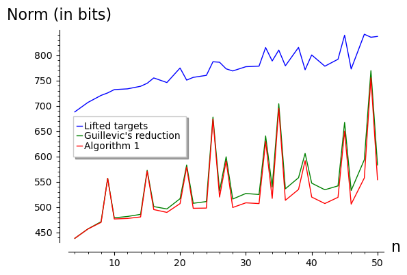
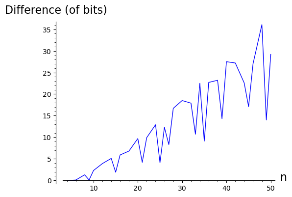
Figure 3: Average norms in the number field of the lifted targets, of Guillevic’s candidates and of candidates from Algorithm 1, as a function of the extension degree $n$. Experiments run on approximately 500-bit finite fields.

    Figure 4: Difference of sizes in basis 2 between the average norms of Guillevic’s candidates and the average norms of candidates from Algorithm 1, as a function of the extension degree $n$. Experiments run on approximately 500-bit finite fields.

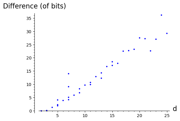
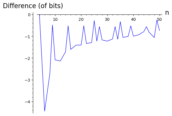
Figure 5: Difference of sizes in basis 2 between the average norms of Guillevic’s candidates and the average norms of candidates from Algorithm 1, as a function of $d$ the greatest proper divisor of $n$. Experiments run on approximately 500-bit finite fields.

    Figure 6: Difference of sizes in basis 2 between the average Euclidean norms of Guillevic’s candidates and the average Euclidean norms of candidates from Algorithm 1, as a function of the extension degree $n$. Experiments run on approximately 500-bit finite fields.

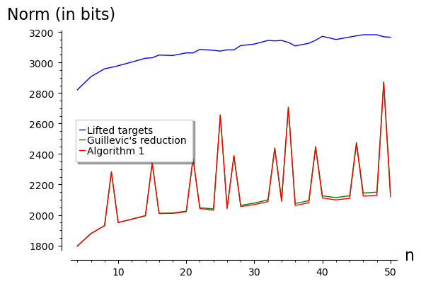
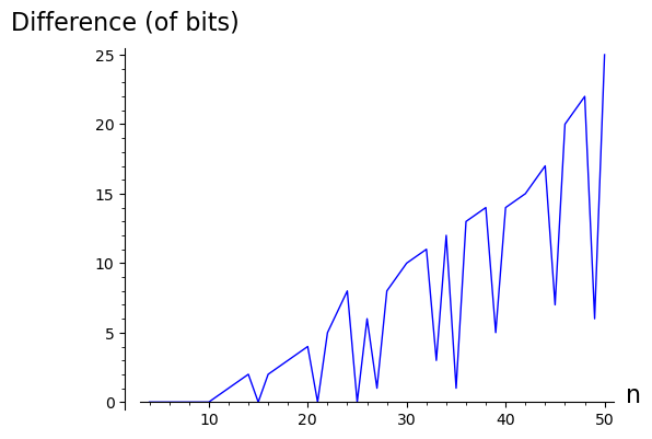
Figure 7: Average norms in the number field of the lifted targets, of Guillevic’s candidates and of candidates from Algorithm 1, as a function of the extension degree $n$. Experiments run on approximately 2048-bit finite fields.

    Figure 8: Difference of sizes in basis 2 between the average norms of Guillevic’s candidates and the average norms of candidates from Algorithm 1, as a function of the extension degree $n$. Experiments run on approximately 2048-bit finite fields.

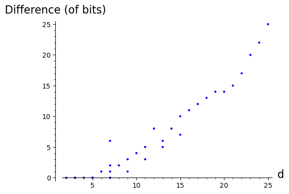
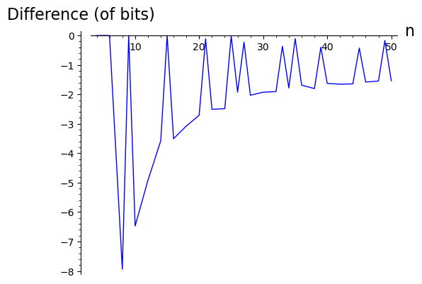
Figure 9: Difference of sizes in basis 2 between the average norms of Guillevic’s candidates and the average norms of candidates from Algorithm 1, as a function of $d$ the greatest proper divisor of $n$. Experiments run on approximately 2048-bit finite fields.

    Figure 10: Difference of sizes in basis 2 between the average Euclidean norms of Guillevic’s candidates and the average Euclidean norms of candidates from Algorithm 1, as a function of the extension degree $n$. Experiments run on approximately 2048-bit finite fields.

Conclusion

We proved that using BKZ reduction instead of LLL lowers the individual logarithm complexity in the lower half of the medium characteristic range.

In addition, experiments show that using sublattices to perform the smoothness step in the number field sieve can outperform the existing technique of using the whole lattice. This new technique outperforms the later when the composite extension degree is sufficiently large and the coefficients of the polynomial constructing the number field are large enough. For instance, these two conditions are fulfilled when dealing with medium characteristic finite fields and using the JLSV₁ polynomial selection. This set up is relevant since the JLSV₁ polynomial selection is both adapted in theory and in practice for TNFS and is well adapted for MNFS in the medium characteristic case, especially when one asks for a symmetric diagram. Such setting can be very useful for the MexTNFS variant in order to get many number fields of the same quality.

Declaration

• Funding: Haetham Al Aswad is funded by French Ministry of Army - AID Agence de l’Innovation de Défense. Cécile Pierrot did not receive support from any organization for the submitted work.

• Financial interests: The authors declare they have no financial interests.

The datasets generated during the study are available in the ”Smoothing step in NFS for composite extension degree finite fields” git lab repository, [AP22].

Appendix 0.A Example

We give a concrete example to better understand Algorithm 1 and to see how decreasing the degree while allowing larger coefficients can result is smaller norms. Take the finite field ${\mathbb{F}}_{p^{28}}$ of size $476$ bits where $p=131101$.

Construction of finite field and number fields:

After running JLSV₁ polynomial selection to find 100 pairs of suitable polynomials. We choose the pair with the highest score for a notion of score based on the alpha value [GS21] and the coefficient sizes. The code to select the pair of polynomials can be found at [AP22].

$f_{1}(X)=X^{28}+349X^{27}+348X^{26}+1040X^{25}+349X^{24}+348X^{23}+1040X^{22}+1040X^{21}+695X^{20}+1041X^{19}+695X^{18}+347X^{17}+349X^{16}+347X^{15}+348X^{14}+694X^{13}+1039X^{12}+348X^{11}+347X^{10}+348X^{9}+1039X^{8}+347X^{7}+695X^{6}+1041X^{5}+349X^{4}+1039X^{3}+347X^{2}+1041X+349$.

$f_{2}(X)=-379X^{28}-1170X^{27}-791X^{26}-857X^{25}-1170X^{24}-791X^{23}-857X^{22}-857X^{21}-1203X^{20}-1236X^{19}-1203X^{18}-412X^{17}-1170X^{16}-412X^{15}-791X^{14}-824X^{13}-478X^{12}-791X^{11}-412X^{10}-791X^{9}-478X^{8}-412X^{7}-1203X^{6}-1236X^{5}-1170X^{4}-478X^{3}-412X^{2}-1236X-1170$.

Moreover, $f_{1}$ is also irreducible in ${\mathbb{F}}_{p}[X]$, thus ${\mathbb{F}}_{p^{28}}$ is represented as:

$${\mathbb{F}}_{p}[X]/(f_{1}):={\mathbb{F}}_{p}(\alpha).$$

Since $f_{1}$ has smaller coefficients than $f_{2}$, it is natural to perform the smoothing step in $\mathcal{K}={\mathbb{Q}}[X]/(f_{1}):={\mathbb{Q}}(x)$. Denote by $\mathcal{N}$ the norm defined in $\mathcal{K}$ and for any element $Y$ in ${\mathbb{F}}_{p}(\alpha)$, $\bar{Y}$ denotes its natural preimage in $\mathcal{K}$.

Generator selection:

Finding a generator of ${\mathbb{F}}_{p^{n}}^{*}$ requires factoring $p^{n}-1$ which is out of reach. Instead one chooses a random element $g\in{\mathbb{F}}_{p^{n}}^{*}$ and tests if $g^{(p^{n}-1)/m}\not=1$ for all $m$ running over small divisors of $p^{n}-1$ (say all divisors smaller than $10^{9}$). Such an element has a very high probability of being a generator of ${\mathbb{F}}_{p^{n}}^{*}$, and is called a pseudo generator. Running our code that is available at [AP22], we find the following pseudo generator of ${\mathbb{F}}_{p^{28}}^{*}$: $g=44501\alpha^{27}+17288\alpha^{26}+79714\alpha^{25}+15355\alpha^{24}+100146\alpha^{23}+87012\alpha^{22}+18126\alpha^{21}+125995\alpha^{20}+12941\alpha^{19}+86746\alpha^{18}+22260\alpha^{17}+8816\alpha^{16}+41799\alpha^{15}+19116\alpha^{14}+45121\alpha^{13}+116926\alpha^{12}+11767\alpha^{11}+64435\alpha^{10}+16296\alpha^{9}+33812\alpha^{8}+96819\alpha^{7}+40474\alpha^{6}+105343\alpha^{5}+71563\alpha^{4}+48599\alpha^{3}+102954\alpha^{2}+36712\alpha+3594$.

Target selection:

We choose a target constructed from the decimal digits of $\pi$.

$T=1415926\alpha^{27}+5358979\alpha^{26}+3238462\alpha^{25}+6433832\alpha^{24}+7950288\alpha^{23}+4197169\alpha^{22}+3993751\alpha^{21}+582097\alpha^{20}+4944592\alpha^{19}+3078164\alpha^{18}+628620\alpha^{17}+8998628\alpha^{16}+348253\alpha^{15}+4211706\alpha^{14}+7982148\alpha^{13}+865132\alpha^{12}+8230664\alpha^{11}+7093844\alpha^{10}+6095505\alpha^{9}+8223172\alpha^{8}+5359408\alpha^{7}+1284811\alpha^{6}+1745028\alpha^{5}+4102701\alpha^{4}+9385211\alpha^{3}+555964\alpha^{2}+4622948\alpha+9549303$.

After reducing each coefficient modulo $p$, the target $T$ becomes: $T=104916\alpha^{27}+114939\alpha^{26}+92038\alpha^{25}+9883\alpha^{24}+84228\alpha^{23}+1937\alpha^{22}+60721\alpha^{21}+57693\alpha^{20}+93855\alpha^{19}+62841\alpha^{18}+104216\alpha^{17}+83760\alpha^{16}+86051\alpha^{15}+16474\alpha^{14}+116088\alpha^{13}+78526\alpha^{12}+102402\alpha^{11}+14390\alpha^{10}+64859\alpha^{9}+94910\alpha^{8}+115368\alpha^{7}+104902\alpha^{6}+40715\alpha^{5}+38570\alpha^{4}+77040\alpha^{3}+31560\alpha^{2}+34413\alpha+110031$.

Outputs:

To run our code [AP22], one starts by creating an instance from smoothness.sage: diag = Smoothness(p, n, f1, f1, g), and then one calls the method smoothness_lattice_n: $R_{1}$, $R_{2}$, $s_{best}$ = diag.smoothness_lattice_n(T). We get $\overline{R_{1}}$ the output of the algorithm of [Gui19] (i.e: Algorithm 1 with $s=0$) and $\overline{R_{2}}$ the output of Algorithm 1 for the best choice of $s$, that is $s_{practical}$. We recall that $s_{practical}$ is the number of columns erased from the lattice that results in the output of the smallest element, that is $\overline{R_{2}}$. We get:

$\overline{R_{1}}=-13x^{27}-51x^{26}-10x^{25}+100x^{24}+219x^{23}+80x^{22}+98x^{21}+54x^{20}-5x^{19}+113x^{18}-195x^{17}+92x^{16}-46x^{15}-99x^{14}+9x^{13}+77x^{12}-173x^{11}+77x^{10}+57x^{9}+213x^{8}-82x^{7}-107x^{6}-76x^{5}-58x^{4}-8x^{3}+34x^{2}-64x-28$.

$\overline{R_{2}}=175x^{23}-87x^{22}-10x^{21}+305x^{20}+233x^{19}-37x^{18}-151x^{17}-123x^{16}-30x^{15}+105x^{14}+145x^{13}-214x^{12}+143x^{11}+432x^{10}+63x^{9}-222x^{8}-17x^{7}-303x^{6}-309x^{5}-239x^{4}+25x^{3}-373x^{2}-330x-174$, where $s_{practical}=4$.

Norms of the target and the outputs:

The norm of the target is $\mathcal{N}\left(\bar{T}\right)\approx 2^{769}$, the norm of $\overline{R_{1}}$ is $\mathcal{N}\left(\overline{R_{1}}\right)\approx 2^{507}$, and the norm of $R_{2}$ is $\mathcal{N}\left(\overline{R_{2}}\right)\approx 2^{492}$. Our algorithm outputs here an element of norm 15 bits smaller than the one output by [Gui19]. We emphasize that $\overline{R_{1}}$ is of degree maximal $27$ whereas $\overline{R_{2}}$ is of degree $27-4=23$ and has slightly larger coefficients.

Probability of smoothness:

Fix a smoothness bound $B=2^{35}$. Then using the dickman_rho function implemented is sage, the probability of $\mathcal{N}\left(\overline{R_{1}}\right)$ being $B$-smooth is about $6.45\times 10^{-19}$ and the probability of $\mathcal{N}\left(\overline{R_{2}}\right)$ being $B$-smooth is about $3.77\times 10^{-18}$. Our output is $5.8$ more likely to be smooth.

Larger example:

As shown in Section 6, our algorithm performs the best as the degree extension $n$ grows. For instance let us look at the $2050$-bits finite field ${\mathbb{F}}_{p^{n}}={\mathbb{F}}_{2199023255579^{50}}$. All the parameters for this setting, such as the polynomials selected and the generator, can be found in the GitLab repository [AP22]. Similarly as above, applying Algorithm 1 leads to the following:

1. The norm of the target chosen with the decimals of $\pi$ is $\mathcal{N}\left(\overline{T}\right)\approx 2^{3152}$

2. The norm of the output $\overline{R_{1}}$ of [Gui19]’s algorithm is $\mathcal{N}\left(\overline{R_{1}}\right)\approx 2^{2138}$

3. The norm of the output $\overline{R_{2}}$ of Algorithm 1 with the best $s$ is $\mathcal{N}\left(\overline{R_{2}}\right)\approx 2^{2121}$, where the best $s$ is $s_{practical}=4$.

In this example our output is $2^{17}$ times smaller. If the smoothness bound is set to $B=2^{70}$, then our output is about $3.5$ times more likely to be $B$-smooth. Since the smoothness probability is higher, one can set a lower smoothness bound in order to get a smaller descent tree.

Appendix 0.B Data

The next two tables present the results of our experiments: $n$ is the extension degree, $d$ is the largest divisor of $n$, $p$ in bits is the number of bits of the characteristic $p$, Bitsize of the field is the size of the finite field ${\mathbb{F}}_{p^{n}}$ in bits, Input norms in bits is the mean in bits of the norms in the number field of the 1000 targets, Output norms with [Guil19] in bits is the mean in bits of the norms output by [Guil19], Our norms in bits is the mean in bits of the norms output by Algorithm $1$, $s_{practical}$ is the mean of the best choice of $s$ in Algorithm $1$ in practice rounded to one decimal place, and $s_{theoretical}$ is the optimal $s$ given from the asymptotic formula rounded to the integer below. Each given norm in a given finite field is a mean of the norms of 1000 elements. The data is sorted in respect to $n$ the extension degree. Moreover, the polynomials selected for the experiments, the pseudo generators of the multiplicative group in each finite field, and the implementation that produced this data are available at [AP22].

n	d	p in bits	Bitsize of	Input norms	Output norms	Our norms	$s_{practical}$	$s_{theoretical}$
			the field	in bits	with [Gui19] in bits	in bits
4	2	125	500	688	438	438	0.0	0
6	3	83	498	707	457	457	0.1	0
8	4	62	496	721	471	470	0.3	0
9	3	55	495	726	557	557	0.0	0
10	5	50	500	732	479	477	0.4	0
12	6	41	492	734	482	478	0.7	0
14	7	35	490	739	486	481	0.9	0
15	5	33	495	745	573	571	0.2	0
16	8	31	496	755	501	495	1.2	0
18	9	27	486	746	497	490	1.4	0
20	10	25	500	775	517	507	1.7	0
21	7	23	483	751	583	579	0.6	0
22	11	22	484	757	508	498	2.1	0
24	12	20	480	761	511	498	2.5	2
25	5	20	500	787	678	674	0.4	0
26	13	19	494	786	532	520	2.8	3
27	9	18	486	773	600	591	1.1	1
28	14	17	476	769	516	499	3.2	6
30	15	16	480	778	527	509	3.9	8
32	16	15	480	779	525	507	4.2	10
33	11	15	495	815	641	630	1.8	7
34	17	14	476	789	540	517	5.0	12
35	7	14	490	810	704	695	1.1	5
36	18	13	468	779	536	514	5.5	14
38	19	13	494	816	558	535	5.7	15
39	13	12	468	772	606	592	2.7	11
40	20	12	480	801	548	520	6.5	18
42	21	11	462	779	534	507	7.2	19
44	22	11	484	792	542	520	6.9	20
45	15	11	495	840	668	651	4.0	13
46	23	10	460	773	533	506	8.2	21
48	24	10	480	842	594	558	10.4	22
49	7	10	490	836	770	756	2.5	5
50	25	10	500	837	584	554	8.8	23

Table 3: Experiments are run on 460 to 500-bit finite fields. The extension degree varies from $4$ to $50$.

n	d	p in bits	Bitsize of	Input norms	Output norms	Our norms	$s_{practical}$	$s_{theoretical}$
			the field	in bits	with [Gui19] in bits	in bits
4	2	513	2052	2821	1796	1796	0.0	0
6	3	342	2052	2907	1878	1878	0.0	0
8	4	257	2056	2959	1930	1930	0.0	0
9	3	228	2052	2968	2282	2282	0.0	0
10	5	205	2050	2979	1950	1950	0.0	0
12	6	171	2052	3003	1973	1972	0.1	0
14	7	147	2058	3028	1996	1994	0.2	0
15	5	137	2055	3031	2342	2342	0.0	0
16	8	129	2064	3049	2011	2009	0.3	0
18	9	114	2052	3046	2013	2010	0.5	0
20	10	103	2060	3063	2025	2021	0.6	0
21	7	98	2058	3063	2370	2370	0.0	0
22	11	94	2068	3086	2047	2042	0.7	0
24	12	86	2064	3080	2040	2032	0.8	0
25	5	82	2050	3075	2656	2656	0.0	0
26	13	79	2054	3083	2047	2041	0.8	0
27	9	76	2052	3083	2389	2388	0.1	0
28	14	74	2072	3111	2063	2055	1.0	0
30	15	69	2070	3121	2078	2068	1.1	0
32	16	65	2080	3145	2099	2088	1.3	0
33	11	63	2079	3142	2440	2437	0.2	0
34	17	61	2074	3145	2101	2089	1.4	0
35	7	59	2065	3132	2707	2706	0.1	0
36	18	57	2052	3109	2075	2062	1.6	0
38	19	54	2052	3126	2094	2080	1.9	0
39	13	53	2067	3146	2449	2444	0.3	0
40	20	52	2080	3172	2125	2111	1.9	0
42	21	49	2058	3151	2114	2099	2.2	0
44	22	47	2068	3167	2126	2109	2.4	0
45	15	46	2070	3175	2476	2469	0.5	0
46	23	45	2070	3182	2144	2124	2.6	0
48	24	43	2064	3182	2150	2128	2.9	2
49	7	42	2058	3169	2873	2867	0.2	0
50	25	41	2050	3166	2144	2119	3.2	4

Table 4: Experiments are run on 2050 to 2080-bit finite fields. The extension degree varies from $4$ to $50$.

References

- [AP22] Haetham Al Aswad and Cécile Pierrot. Smoothness step in NFS for composite extenion finite fields. https://gitlab.inria.fr/halaswad/smoothing-step-in-nfs-for-composite-extension-degree-finite-fields. GitLab, 2022.
- [BF01] Dan Boneh and Matthew K. Franklin. Identity-based encryption from the Weil pairing. In Joe Kilian, editor, CRYPTO 2001, volume 2139 of LNCS, pages 213–229. Springer, Heidelberg, August 2001.
- [BFHMV84] Ian Blake, R. Fuji-Hara, R. Mullin, and S. Vanstone. Computing logarithms in finite fields of characteristic two. Siam Journal on Algebraic and Discrete Methods, 5, 06 1984.
- [BGG+20] Fabrice Boudot, Pierrick Gaudry, Aurore Guillevic, Nadia Heninger, Emmanuel Thomé, and Paul Zimmermann. Comparing the difficulty of factorization and discrete logarithm: A 240-digit experiment. In Hovav Shacham and Alexandra Boldyreva, editors, CRYPTO 2020, Part II, LNCS, pages 62–91. Springer, Heidelberg, August 2020.
- [BGGM15a] Razvan Barbulescu, Pierrick Gaudry, Aurore Guillevic, and François Morain. DL record computation in of bits, 2015. http://www.lix.polytechnique.fr/~guillevic/docs/guillevic-catrel15-talk.pdf.
- [BGGM15b] Razvan Barbulescu, Pierrick Gaudry, Aurore Guillevic, and François Morain. Improving NFS for the discrete logarithm problem in non-prime finite fields. In Elisabeth Oswald and Marc Fischlin, editors, EUROCRYPT 2015, Part I, volume 9056 of LNCS, pages 129–155. Springer, Heidelberg, April 2015.
- [BGJT14] Razvan Barbulescu, Pierrick Gaudry, Antoine Joux, and Emmanuel Thomé. A heuristic quasi-polynomial algorithm for discrete logarithm in finite fields of small characteristic. In Phong Q. Nguyen and Elisabeth Oswald, editors, EUROCRYPT 2014, volume 8441 of LNCS, pages 1–16. Springer, Heidelberg, May 2014.
- [BGK15] Razvan Barbulescu, Pierrick Gaudry, and Thorsten Kleinjung. The tower number field sieve. In Tetsu Iwata and Jung Hee Cheon, editors, ASIACRYPT 2015, Part II, volume 9453 of LNCS, pages 31–55. Springer, Heidelberg, November / December 2015.
- [BLS01] Dan Boneh, Ben Lynn, and Hovav Shacham. Short signatures from the Weil pairing. In Colin Boyd, editor, ASIACRYPT 2001, volume 2248 of LNCS, pages 514–532. Springer, Heidelberg, December 2001.
- [BMV84] Ian F. Blake, Ronald C. Mullin, and Scott A. Vanstone. Computing logarithms in . In G. R. Blakley and David Chaum, editors, CRYPTO’84, volume 196 of LNCS, pages 73–82. Springer, Heidelberg, August 1984.
- [BP14] Razvan Barbulescu and Cécile Pierrot. The Multiple Number Field Sieve for Medium and High Characteristic Finite Fields. LMS Journal of Computation and Mathematics, 17:230–246, 2014.
- [CEP83] E. Rodney Canfield, Paul Erdös, and Carl Pomerance. On a problem of Oppenheim concerning “factorisatio numerorum”. Journal of Number Theory, 17(1):1–28, 1983.
- [FP85] Ulrich Fincke and Michael E. Pohst. Improved methods for calculating vectors of short length in a lattice. Mathematics of Computation, 1985.
- [GKZ14] Robert Granger, Thorsten Kleinjung, and Jens Zumbrägel. Breaking ‘128-bit secure’ supersingular binary curves - (or how to solve discrete logarithms in and ). In Juan A. Garay and Rosario Gennaro, editors, CRYPTO 2014, Part II, volume 8617 of LNCS, pages 126–145. Springer, Heidelberg, August 2014.
- [Gré] Laurent Grémy. Computations of discrete logarithms sorted by date. https://dldb.loria.fr/.
- [GS21] Aurore Guillevic and Shashank Singh. On the Alpha Value of Polynomials in the Tower Number Field Sieve Algorithm. Mathematical Cryptology, 1(1):39, 2021.
- [Gui15] Aurore Guillevic. Computing individual discrete logarithms faster in with the NFS-DL algorithm. In Tetsu Iwata and Jung Hee Cheon, editors, ASIACRYPT 2015, Part I, volume 9452 of LNCS, pages 149–173. Springer, Heidelberg, November / December 2015.
- [Gui19] Aurore Guillevic. Faster individual discrete logarithms in finite fields of composite extension degree. Mathematics of Computation, 88(317):1273–1301, January 2019.
- [HPS11] Guillaume Hanrot, Xavier Pujol, and Damien Stehlé. Analyzing blockwise lattice algorithms using dynamical systems. In Phillip Rogaway, editor, CRYPTO 2011, volume 6841 of LNCS, pages 447–464. Springer, Heidelberg, August 2011.
- [JLSV06] Antoine Joux, Reynald Lercier, Nigel Smart, and Frederik Vercauteren. The number field sieve in the medium prime case. In Cynthia Dwork, editor, CRYPTO 2006, volume 4117 of LNCS, pages 326–344. Springer, Heidelberg, August 2006.
- [Jou04] Antoine Joux. A one round protocol for tripartite Diffie-Hellman. Journal of Cryptology, 17(4):263–276, 2004.
- [JP14] Antoine Joux and Cécile Pierrot. The special number field sieve in - application to pairing-friendly constructions. In Zhenfu Cao and Fangguo Zhang, editors, PAIRING 2013, volume 8365 of LNCS, pages 45–61. Springer, Heidelberg, November 2014.
- [Kan87] Ravi Kannan. Minkowski’s convex body theorem and integer programming. Mathematics of Operations Research, 12(3):415–440, aug 1987.
- [KB16] Taechan Kim and Razvan Barbulescu. Extended tower number field sieve: A new complexity for the medium prime case. In Matthew Robshaw and Jonathan Katz, editors, CRYPTO 2016, Part I, volume 9814 of LNCS, pages 543–571. Springer, Heidelberg, August 2016.
- [KJ17] Taechan Kim and Jinhyuck Jeong. Extended tower number field sieve with application to finite fields of arbitrary composite extension degree. In Serge Fehr, editor, PKC 2017, Part I, volume 10174 of LNCS, pages 388–408. Springer, Heidelberg, March 2017.
- [KW19] Thorsten Kleinjung and Benjamin Wesolowski. Discrete logarithms in quasi-polynomial time in finite fields of fixed characteristic. Cryptology ePrint Archive, Report 2019/751, 2019. https://eprint.iacr.org/2019/751.
- [LLL82] A. K. Lenstra, H. W. Lenstra, and L. Lovasz. Factoring Polynomials with Rational Coefficients. Mathematische Annalen, 261:515–534, 1982.
- [MGP21] Gabrielle De Micheli, Pierrick Gaudry, and Cécile Pierrot. Lattice enumeration for tower NFS: A 521-bit discrete logarithm computation. In Mehdi Tibouchi and Huaxiong Wang, editors, Advances in Cryptology - ASIACRYPT 2021 - 27th International Conference on the Theory and Application of Cryptology and Information Security, Singapore, December 6-10, 2021, Proceedings, Part I, volume 13090 of Lecture Notes in Computer Science, pages 67–96. Springer, 2021.
- [Mil04] Victor Miller. The Weil pairing, and its efficient calculation. Journal of Cryptology, 17:235–261, 2004.
- [MS20] Madhurima Mukhopadhyay and Palash Sarkar. Faster initial splitting for small characteristic composite extension degree fields. Finite Fields and Their Applications, 62:101629, 2020.
- [MSST22] Madhurima Mukhopadhyay, Palash Sarkar, Shashank Singh, and Emmanuel Thomé. New discrete logarithm computation for the medium prime case using the function field sieve. Advances in Mathematics of Communications, 16(3):449–464, 2022.
- [MV10] Daniele Micciancio and Panagiotis Voulgaris. A deterministic single exponential time algorithm for most lattice problems based on voronoi cell computations. In Leonard J. Schulman, editor, 42nd ACM STOC, pages 351–358. ACM Press, June 2010.
- [MW15] Daniele Micciancio and Michael Walter. Fast lattice point enumeration with minimal overhead. In Piotr Indyk, editor, 26th SODA, pages 276–294. ACM-SIAM, January 2015.
- [MW16] Daniele Micciancio and Michael Walter. Practical, predictable lattice basis reduction. In Marc Fischlin and Jean-Sébastien Coron, editors, EUROCRYPT 2016, Part I, volume 9665 of LNCS, pages 820–849. Springer, Heidelberg, May 2016.
- [Pie15] Cécile Pierrot. The multiple number field sieve with conjugation and generalized Joux-Lercier methods. In Elisabeth Oswald and Marc Fischlin, editors, EUROCRYPT 2015, Part I, volume 9056 of LNCS, pages 156–170. Springer, Heidelberg, April 2015.
- [Sch00] Oliver Schirokauer. Using Number Fields to Compute Logarithms in Finite Fields. Mathematics of Computation, 69:1267–1283, 2000.
- [SE94] Claus-Peter Schnorr and M. Euchner. Lattice basis reduction: Improved practical algorithms and solving subset sum problems. Mathematical Programming, 66:181–199, 1994.
- [SS16] Palash Sarkar and Shashank Singh. A general polynomial selection method and new asymptotic complexities for the tower number field sieve algorithm. In Jung Hee Cheon and Tsuyoshi Takagi, editors, ASIACRYPT 2016, Part I, volume 10031 of LNCS, pages 37–62. Springer, Heidelberg, December 2016.
- [SS19] Palash Sarkar and Shashank Singh. A unified polynomial selection method for the (tower) number field sieve algorithm, 2019.
- [TPM] Trusted platform module. https://trustedcomputinggroup.org/resource/tpm-library-specification/. Latest Version Nov. 2019.
- [Wie86] Douglas H. Wiedemann. Solving Sparse Linear Equations over Finite Fields. IEEE Transactions on Information Theory, 32(1):54–62, 1986.