A numerical framework for simulating progressive failure in composite laminates under high-cycle fatigue loading

Abstract

In this work, a recently proposed high-cycle fatigue cohesive zone model, which covers crack initiation and propagation with limited input parameters, is embedded in a robust and efficient numerical framework for simulating progressive failure in composite laminates under fatigue loading. The fatigue cohesive zone model is enhanced with an implicit time integration scheme of the fatigue damage variable which allows for larger cycle increments and more efficient analyses. The method is combined with an adaptive strategy for determining the cycle increment based on global convergence rates. Moreover, a consistent material tangent stiffness matrix has been derived by fully linearizing the underlying mixed-mode quasi-static model and the fatigue damage update. The enhanced fatigue cohesive zone model is used to describe matrix cracking and delamination in laminates. In order to allow for matrix cracks to initiate at arbitrary locations and to avoid complex and costly mesh generation, the phantom node version of the eXtended finite element method (XFEM) is employed. For the insertion of new crack segments, an XFEM fatigue crack insertion criterion is presented, which is consistent with the fatigue cohesive zone formulation. It is shown with numerical examples that the improved fatigue damage update enhances the accuracy, efficiency and robustness of the numerical simulations significantly. The numerical framework is applied to the simulation of progressive fatigue failure in an open-hole [$\pm 45$]-laminate. It is demonstrated that the numerical model is capable of accurately and efficiently simulating the complete failure process from distributed damage to localized failure.

Keywords: composite laminates; high-cycle fatigue, progressive failure; extended finite element method, cohesive zone modeling

 

1.   Introduction

Fatigue is often a critical failure process in fiber reinforced polymer laminates. Accurate, efficient and robust numerical prediction tools can help in enhancing the efficiency of the design process of composite laminated structures, reducing manufacturing time, and minimizing the need for extensive testing to ensure the safety of new composite structures.

When fiber reinforced polymer laminates are subjected to loads, several interacting failure processes take place that make developing reliable prediction tools a challenging endeavor. For example, matrix cracks can initiate and propagate and eventually lead to interface delamination. Finally, fiber breakage can occur leading to overall failure of the laminate. The interaction of these competing processes and the type of final failure depend on the stacking sequence, laminate thickness and the presence of notches [1, 2]. Furthermore, the load character (cyclic or quasi-static) influences the final failure mode [3, 3, 4, 5]. In addition, damage accumulation in fiber reinforced composite materials already takes place at an early stage which results in significant stiffness reduction and stress redistribution. In order to accurately predict the performance of composite laminates, numerical models must take into account the progressive character of failure that covers the initial stage of early damage up to complete failure of the laminate.

In literature, several numerical models have been developed for the quasi-static load case of complex laminates. For example, Jiang et al. [6] modelled splitting and matrix cracks with interface elements at pre-defined locations according to experiments. Hallet et al. [7] used a similar approach for matrix cracks and delamination and included a Weibull statistical criterion for fiber failure. Furthermore, Van der Meer et al. [8, 9] used the phantom node version of the extended finite element method (XFEM) [10] for modeling matrix cracks to reduce the complexity of meshing and to allow for mesh-independent cracks that can initiate at arbitrary locations with a pre-defined crack spacing. Moreover, [11] [11] used a 3D version of the floating node method [12] to model the interaction of a large number of discrete matrix cracks with delaminations and demonstrated that the model was able to accurately predict the sequence of failure processes in notched and unnotched laminates. More modeling approaches of composite laminates subjected to quasi-static loading scenarios can be found in Refs. [13, 14, 15, 16, 17, 18, 19, 20, 21, 22]

At present, there are only few progressive failure models that can simulate (high-cycle) fatigue failure in composite laminates. One of the first papers of open-hole fatigue modeling of progressive failure was presented by Nixon-Pearson et al. [23], where pre-inserted interface elements were used to model matrix cracks and a Paris-type cyclic cohesive zone model (CZM) [24, 25] was used for crack propagation. Iarve et al. [17] developed a model where the regularized eXtended finite element method (Rx-FEM) was employed for modeling mesh-independent cracks and a fatigue initiation criterion based on S-N curves was presented. This framework was further extended by [26] [26] to account for high-density crack networks by allowing cracks to appear close to each other. In the work by Tao et al. [27], a similar approach as in [23] [23] was adopted, but extended with a fatigue initiation criterion based on S-N curves, similar as proposed in Ref. [17]. As opposed to the discrete crack modeling approaches for simulating matrix cracking in the previously mentioned approaches, Llobet et al. [28] used a continuum damage modeling approach with fiber-aligned meshes and included a description for fiber damage due to cyclic loading. More recently, [29] [29] developed an enhanced fatigue cohesive zone model where stiffness degradation is described by a Paris-relation-informed neural network and applied it to simulate an open-hole fatigue tension test with good accuracy.

In most of the existing methods, a fatigue cohesive zone model, that requires a Paris-relation [30] as input, is used for modeling delamination and matrix cracking. These cohesive zone models are suitable for describing crack propagation of an initial crack [31, 24, 25, 32, 33, 34, 35, 36]. However, in full-laminate analysis, a matrix crack can also initiate under cyclic loading. Upon further applying fatigue load cycles, a fracture process zone develops in the onset phase after which propagation of the crack takes place. In literature, only a few CZMs take these three stages of fatigue crack growth into account [37, 17, 26, 38, 39, 40, 28].

Recently, Dávila [37] proposed a cyclic CZM that covers initiation, onset and propagation and is built on Turon’s quasi-static mixed-mode CZM [41, 42]. The fatigue CZM relies on S-N curves with simple engineering assumptions and empirical relations to take the dependence of mode-mixity and stress-ratio into account. The method is based on the assumption that an intrinsic relation exists between S-N curves and Paris’ relation [43]. The model is capable of simulating complex 3D crack fronts [44] in a reinforced double cantilever beam (DCB) test [45] and can be extended to cases where the local stress ratio is not equal to the global load ratio, as presented in [46] where the presence of residual stresses was taken into account. Furthermore, it has been demonstrated that the method can simulate crack migration in a ply-drop specimen [47] and R-curve effects in thermoplastic material systems [48]. With regards to laminate analyses, the unification of initiation and propagation makes the fatigue CZM suitable for simulating both interface delamination and matrix cracking in progressive failure analyses of complex laminates.

Originally, the model presented in Ref. [37] employed an explicit update of the damage variable that evolves with load cycles. Therefore, small cycle increments must be used during simulations to prevent instabilities in the damage evolution and a step size criterion based on the maximum damage experienced in all integration points is required. This approach may become problematic in full-laminate analyses where many integration points, due to stress redistribution and complex loading histories, experience different damage rates throughout the simulation.

In this work, an implicit fatigue damage update is presented to make the formulation more suitable for use in full-laminate analyses. The method is combined with efficient cycle jumping based on global iterations and a fully consistent tangent matrix has been derived to enhance efficiency and robustness of the simulations. In order to allow for multiple cracks at arbitrary locations, the fatigue CZM is combined with XFEM with a proper fatigue crack insertion criterion that is consistent with the fatigue damage evolution.

The organization of this article is as follows. Firstly the improvement to Dávila’s fatigue damage formulation is presented and a fully consistent material tangent is derived. Subsequently, the XFEM implementation with a proper fatigue crack insertion criterion is presented. The model is applied to several numerical examples to verify the methods and to the show the improved performance. In order to demonstrate the capabilities of the presented numerical framework, an open-hole [$\pm$45]-laminate under fatigue loading is simulated.

2.   Methods

2.1.   Fatigue cohesive zone model

The fatigue CZM by Dávila [37, 49] is built on top of the static CZM with mode-dependent dummy stiffness by Turon [41, 42]. In this section, the formulation of the fatigue CZM is given in local coordinate frame with basis vectors $\{\bm{e}_{n},\bm{e}_{s1},\bm{e}_{s2}\}$ aligned with the crack plane.

In order to allow for a reduction of elastic stiffness due to fatigue and static loading, a scalar damage variable $d$ is introduced. The traction is computed as

$$\textbf{t}=(\textbf{I}-d\textbf{P})\textbf{K}\llbracket\textbf{u}\rrbracket$$ (1)

where $\llbracket\textbf{u}\rrbracket$ is the displacement jump, K is the dummy stiffness matrix and P is a selection matrix expressed as

$$\textbf{K}=\begin{bmatrix}K_{n}&0&0\\ 0&K_{sh}&0\\ 0&0&K_{sh}\end{bmatrix},$$ (2)

$$\textbf{P}=\begin{bmatrix}\frac{\left<\llbracket u\rrbracket_{n}\right>}{\llbracket u\rrbracket_{n}}&0&0\\ 0&1&0\\ 0&0&1\end{bmatrix}$$ (3)

where $K_{n}$ and $K_{sh}$ are the normal and shear dummy stiffnesses respectively. The operator $\left<\bm{\bullet}\right>$ is the Macaulay operator, defined as $\mathrm{max}(0,\bullet)$ and makes sure that interfacial penetration is prevented when the normal component of the displacement jump is negative. The damage variable $d$ determines the stiffness reduction and its evolution depends on the mode-mixity such that the energy dissipated matches with the phenomenological mixed-mode fracture energy relation proposed by Benzeggagh and Kenane [50]. It is shown in [51, 42] that the correct energy dissipation under mixed-mode fracture is ensured by relating the ratio between dummy stiffnesses $K_{n}$ and $K_{sh}$ to the fracture properties with the following equation

$$K_{sh}=K_{n}\frac{G_{Ic,d}}{G_{IIc,d}}\Bigg{(}\frac{f_{sh}}{f_{n}}\Bigg{)}^{2}$$ (4)

where $f_{n}$, $f_{sh}$, $G_{Ic,d}$ and $G_{IIc,d}$ are the tensile strength, shear strength, mode-I and mode-II fracture energies, respectively. The mixed-mode CZM is formulated in the form of an equivalent 1D traction-separation relation

$$\sigma=(1-d)K_{\mathcal{B}}\Delta$$ (5)

where $\sigma$ is the equivalent stress, $K_{\mathcal{B}}$ is the mode-dependent dummy stiffness and $\Delta$ is the equivalent displacement jump. These quantities are defined as

$$\sigma=\sqrt{\left<t_{n}\right>^{2}+t^{2}_{s1}+t^{2}_{s2}}$$ (6)

$$K_{\mathcal{B}}=K_{n}(1-\mathcal{B})+\mathcal{B}K_{sh}$$ (7)

$$\Delta=\frac{K_{n}\left<\llbracket u\rrbracket_{n}\right>^{2}+K_{sh}\llbracket u\rrbracket_{sh}^{2}}{\sqrt{K_{n}^{2}\left<\llbracket u\rrbracket_{n}\right>^{2}+K_{sh}^{2}\llbracket u\rrbracket_{sh}^{2}}}$$ (8)

where $\mathcal{B}$ is a displacement-based measure of mode-mixity

$$\mathcal{B}=\frac{K_{sh}\llbracket u\rrbracket_{sh}^{2}}{K_{n}\left<\llbracket u\rrbracket_{n}\right>^{2}+K_{sh}\llbracket u\rrbracket_{sh}^{2}}$$ (9)

and $\llbracket u\rrbracket_{sh}$ is the Eucledian norm (length) of the shear displacement jump vector

$$\llbracket u\rrbracket_{sh}^{2}=\llbracket u\rrbracket_{s1}^{2}+\llbracket u\rrbracket_{s2}^{2}$$ (10)

The values of equivalent displacement jump at fracture initiation and complete fracture of the 1D equivalent traction-separation relation (equation 5) are expressed as

$$\Delta_{0}=\sqrt{\frac{K_{n}(\llbracket u\rrbracket^{0}_{n})^{2}+\Big{(}K_{sh}(\llbracket u\rrbracket^{0}_{sh})^{2}-K_{n}(\llbracket u\rrbracket^{0}_{n})^{2}\Big{)}\mathcal{B}^{\eta}}{K_{\mathcal{B}}}}$$ (11)

$$\Delta_{f}=\frac{K_{n}\llbracket u\rrbracket^{0}_{n}\llbracket u\rrbracket^{f}_{n}+\Big{(}K_{sh}\llbracket u\rrbracket^{0}_{sh}\llbracket u\rrbracket^{f}_{sh}-K_{n}\llbracket u\rrbracket^{0}_{n}\llbracket u\rrbracket^{f}_{n}\Big{)}\mathcal{B}^{\eta}}{K_{\mathcal{B}}\Delta_{0}}$$ (12)

where $\eta$ is the Benzeggagh-Kenane interaction parameter. The pure-mode jump components corresponding to fracture initiation and complete fracture are given by

$$\llbracket u\rrbracket^{0}_{n}=\frac{f_{n}}{K_{n}},\qquad\,\leavevmode\nobreak\ \llbracket u\rrbracket^{f}_{n}=\frac{2G_{Ic,d}}{f_{n}}$$ (13)

$$\llbracket u\rrbracket^{0}_{sh}=\frac{f_{sh}}{K_{sh}},\qquad\llbracket u\rrbracket^{f}_{sh}=\frac{2G_{IIc,d}}{f_{sh}}$$ (14)

An energy-based damage variable $\mathcal{D}$ is introduced as the state variable, which is defined as the ratio of dissipated energy $G_{d}$ over the critical mixed-mode energy release rate $G_{c}$

$$\mathcal{D}\equiv\frac{G_{d}}{G_{c}}=\frac{\Delta-\Delta_{f}}{\Delta_{f}-\Delta_{0}}$$ (15)

and can only increase in pseudo time $t$, such that for time step $n$ ($t=t_{n}$):

$$\mathcal{D}(t_{n})=\max\limits_{0\leq\tau\leq t_{n}}\big{(}\mathcal{D}(\tau)\big{)}$$ (16)

The stiffness-based damage variable $d$ in equation 1 is related to the energy-based damage variable through

$$d=1-\frac{(1-\mathcal{D})\Delta_{0}}{\mathcal{D}\Delta_{f}+(1-\mathcal{D})\Delta_{0}}$$ (17)

Dávila’s fatigue damage formulation

Figure 1: Dávila’s fatigue cohesive zone model. The evolution of damage variable $\mathcal{D}$ is such that at constant stress and mode-mixity the time to failure $N_{\mathrm{fail}}$ matches with an S-N curve

Figure 2: Nomenclature of the fatigue CZM. The fatigue traction-separation response (${\color[rgb]{0,0,1}\definecolor[named]{pgfstrokecolor}{rgb}{0,0,1}\bullet}$) is inside the quasi-static envelope

In Dávila’s fatigue CZM, the number of cycles to failure of a 1D bar with a single crack and cyclic load matches with an S-N curve (see figure 1). This is achieved by reducing the stiffness at constant applied stress until the traction-separation response reaches the quasi-static softening line, which marks failure of the material point. The evolution of the energy-based damage variable during fatigue $\mathcal{D}_{f}$ is described with the following (nonlinear) differential equation

$$\derivative{\mathcal{D}_{f}}{N}=f_{\mathcal{D}}(\Delta,\Delta^{*},\mathcal{D})$$ (18)

where $\Delta^{*}$ is the reference displacement, which is the displacement corresponding to the residual traction (see figure 2) and can be computed as

$$\Delta^{*}=\mathcal{D}(\Delta_{f}-\Delta_{0})+\Delta_{0}$$ (19)

The quasi-static damage $\mathcal{D}_{s}$ is computed as

$$\mathcal{D}_{s}=\frac{\Delta-\Delta_{0}}{\Delta_{f}-\Delta_{0}}$$ (20)

and the updated damage is determined as the maximum of the static and the fatigue damage

$$\mathcal{D}=\max\big{(}\mathcal{D}_{s},\mathcal{D}_{f}\big{)}$$ (21)

to ensure that the traction-opening response during fatigue loading is inside the quasi-static envelope.

In [49], several fatigue damage functions were proposed and compared. It was shown that the so-called CF20 damage function

$$f^{\mathrm{CF20}}_{\mathcal{D}}=\frac{1}{\gamma}\frac{(1-\mathcal{D})^{\beta-p}}{E^{\beta}(p+1)}\bigg{(}\frac{\Delta}{\Delta^{*}}\bigg{)}^{\beta}$$ (22)

gave the most satisfactory results. Here, $\gamma$ is the number of cycles to failure at the endurance limit (which is usually set to $10^{7}$ cycles), $p$ can be calibrated such that the propagation rates in the simulation match with (available) Paris curves [49] and $\beta$ is the exponent in the S-N curve, computed as

$$\beta=\frac{-7\eta}{logE}$$ (23)

where $\eta$ is a brittleness parameter that can take into account the low-cycle fatigue response in the S-N curve.

For a given stress ratio $R\equiv\sigma^{\mathrm{min}}/\sigma^{\mathrm{max}}$, the relative endurance limit $E$, defined as the ratio of equivalent endurance limit $\sigma_{\mathrm{end}}$ and mode-dependent static strength $f_{\mathcal{B}}$, is computed from the relative endurance limit $\epsilon$ (at full load reversal $R=-1$) with the Goodmann diagram:

$$E=\frac{2C_{l}\epsilon}{C_{l}\epsilon+1+R(C_{l}\epsilon-1)}$$ (24)

where $C_{l}$ is an empirical relation which takes into account the effect of mode-mixity [52]:

$$C_{l}=1-0.42\mathcal{B}$$ (25)

In summary, the input fatigue model parameters for CF20 are $\eta,\epsilon$ and $p$.

Implicit fatigue damage update

In order to compute the damage at current pseudo time $t_{n}$, the damage rate function in equation 18 must be integrated, which is mathematically expressed as

$$\mathcal{D}_{f}^{t_{n}}=\mathcal{D}^{t_{n-1}}+\int^{t_{n}}_{t_{n-1}}f_{\mathcal{D}}(\Delta,\Delta^{*},\mathcal{D})\,\mathrm{d}N$$ (26)

[37] [37] used an Euler forward (explicit) time integration scheme where the integral is approximated as $\Delta Nf_{\mathcal{D}}^{(n-1)}$, with $f_{\mathcal{D}}^{(n-1)}$ representing $f_{\mathcal{D}}$ evaluated at $t_{n-1}$. In this work, the damage at current time step $n$ (corresponding to time $t_{n}$) is computed with the generalized trapezoidal rule:

$$\mathcal{D}^{(n)}_{f}=\mathcal{D}^{(n-1)}+\Delta N\Big{[}(1-\theta)f_{\mathcal{D}}^{(n-1)}+\theta f_{\mathcal{D}}^{(n)}\Big{]}$$ (27)

with parameter $\theta\in\big{(}0,1\big{]}$. Through equation 22, $f_{\mathcal{D}}^{(n)}$ requires $\mathcal{D}_{f}^{(n)}$, making the update with equation 27 implicit. The resulting nonlinear equation can be solved at local integration point level, e.g. with Newton’s method by performing iterations until a local convergence criterion is met.

Remark

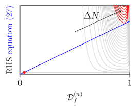
The right-hand side (RHS) of equation 27 depends on the step size $\Delta N$. When the step size is too large and a material point completely fails within the time step, no solution exists for equation 27 (see figure 3). This issue is circumvented by setting $\mathcal{D}_{f}=1$ when this occurs.

Figure 3: Right-hand side of equation 27 as a function of damage $\mathcal{D}_{f}^{(n)}$ (curves in gray) at constant equivalent displacement $\Delta$ while increasing the cycle increment $\Delta N$ starting from $\Delta N=0$ (horizontal gray line). For a given $\Delta N$, the solution of equation 27 is the intersection with the blue line $\mathrm{RHS}=\mathcal{D}_{f}^{(n)}$. The damage value $\mathcal{D}_{0}$ of the previous pseudo time step $n$ is indicated with ${\color[rgb]{1,0,0}\definecolor[named]{pgfstrokecolor}{rgb}{1,0,0}\bullet}$. When the cycle increment is too large, there exists no intersection for $\mathcal{D}_{f}^{(n)}\in\big{[}\mathcal{D}_{0},1\big{)}$ (curves in red).

Consistent linearization of the traction update

In [37] and [42], a numerical tangent stiffness based on finite differences was used to approximate the tangent of the static cohesive relation and the extension with fatigue damage. However, the accuracy of approximating the tangent and robustness depends on the choice of the perturbation and is case-dependent. In addition, the traction update needs to be performed for each perturbation of the displacement jump component, which may not be computationally efficient.

In order to improve the efficiency and robustness, which is crucial in full-laminate analyses, a consistent tangent stiffness matrix is derived below for the static cohesive zone model [42] and the fatigue damage extension [37], including the improved (implicit) fatigue damage update presented in this work.

The traction at current time $n$ is written as a function of displacement jump $\llbracket\textbf{u}\rrbracket$, current damage $\mathcal{D}$ and cycle jump $\Delta N$

$$\textbf{t}=\hat{\textbf{t}}(\llbracket\textbf{u}\rrbracket,\mathcal{D}(\llbracket\textbf{u}\rrbracket,\Delta N))$$ (28)

The linearized traction update can be expressed as

$$\delta\textbf{t}=\underbrace{\Bigg{(}\partialderivative{\hat{\textbf{t}}(\llbracket\textbf{u}\rrbracket,\mathcal{D}(\llbracket\textbf{u}\rrbracket,\Delta N))}{\llbracket\textbf{u}\rrbracket}\Bigg{)}_{(n)}}_{\textbf{D}}\delta\llbracket\textbf{u}\rrbracket$$ (29)

where it is explicitly indicated that the time $n$ is kept constant. The material tangent D can be identified in this expression as the linear operator that maps an iterative-increment of the displacement jump to an iterative-increment of the traction vector.

By performing partial differentiation and after some re-arrangement, the expression of the material tangent becomes

$$\textbf{D}=\underbrace{(\textbf{I}-d\textbf{P})\textbf{K}}_{\mathrm{secant\leavevmode\nobreak\ stiffness}}-\textbf{P}\textbf{K}\llbracket\textbf{u}\rrbracket\partialderivative{d^{{}^{\mathrm{T}}}}{\llbracket\textbf{u}\rrbracket}$$ (30)

Differentiation of the last term in equation 30 and applying the chain rule gives

$$\partialderivative{d}{\llbracket\textbf{u}\rrbracket} =\partialderivative{d}{\mathcal{D}}\partialderivative{\mathcal{D}}{\llbracket\textbf{u}\rrbracket}+\partialderivative{d}{\Delta_{0}}\partialderivative{\Delta_{0}}{\llbracket\textbf{u}\rrbracket}+\partialderivative{d}{\Delta_{f}}\partialderivative{\Delta_{f}}{\llbracket\textbf{u}\rrbracket}$$ (31)

where the partial derivatives $\partial\Delta_{0}/\partial\llbracket\textbf{u}\rrbracket$ and $\partial\Delta_{f}/\partial\llbracket\textbf{u}\rrbracket$ can be further expanded:

$$\partialderivative{\Delta_{0}}{\llbracket\textbf{u}\rrbracket} =\partialderivative{\Delta_{0}}{\mathcal{B}}\partialderivative{\mathcal{B}}{\llbracket\textbf{u}\rrbracket}+\partialderivative{\Delta_{0}}{K_{\mathcal{B}}}\partialderivative{K_{\mathcal{B}}}{\mathcal{B}}\partialderivative{\mathcal{B}}{\llbracket\textbf{u}\rrbracket}$$ (32)

$$\partialderivative{\Delta_{f}}{\llbracket\textbf{u}\rrbracket} =\partialderivative{\Delta_{f}}{\mathcal{B}}\partialderivative{\mathcal{B}}{\llbracket\textbf{u}\rrbracket}+\partialderivative{\Delta_{f}}{K_{\mathcal{B}}}\partialderivative{K_{\mathcal{B}}}{\mathcal{B}}\partialderivative{\mathcal{B}}{\llbracket\textbf{u}\rrbracket}+\partialderivative{\Delta_{f}}{\Delta_{0}}\partialderivative{\Delta_{0}}{\llbracket\textbf{u}\rrbracket}$$ (33)

The partial derivatives in equations 31, 32 and 33 can be computed with quantities already obtained from the traction update algorithm presented before:

$$\partialderivative{d}{\mathcal{D}} =\frac{\Delta_{0}\Delta_{f}}{\big{[}(\mathcal{D}-1)\Delta_{0}-\mathcal{D}\Delta_{f}\big{]}^{2}}$$ (34)

$$\partialderivative{d}{\Delta_{0}} =\frac{(\mathcal{D}-1)\mathcal{D}\Delta_{f}}{\big{[}(\mathcal{D}-1)\Delta_{0}-\mathcal{D}\Delta_{f}\big{]}^{2}}$$ (35)

$$\partialderivative{d}{\Delta_{f}} =\frac{(1-\mathcal{D})\mathcal{D}\Delta_{0}}{\big{[}(\mathcal{D}-1)\Delta_{0}-\mathcal{D}\Delta_{f}\big{]}^{2}}$$ (36)

$$\partialderivative{\Delta_{0}}{\mathcal{B}} =\frac{K_{sh}(\llbracket u\rrbracket^{0}_{sh})^{2}-K_{n}(\llbracket u\rrbracket^{0}_{n})^{2}}{2\Delta_{0}K_{\mathcal{B}}}\mathcal{B}^{\eta-1}\eta$$ (37)

$$\partialderivative{\Delta_{0}}{K_{\mathcal{B}}} =-\frac{\Delta_{0}}{2K_{\mathcal{B}}}$$ (38)

$$\partialderivative{\Delta_{f}}{\mathcal{B}} =\frac{K_{sh}\llbracket u\rrbracket^{0}_{sh}\llbracket u\rrbracket^{f}_{sh}-K_{n}\llbracket u\rrbracket^{0}_{n}\llbracket u\rrbracket^{f}_{n}}{\Delta_{0}K_{\mathcal{B}}}\mathcal{B}^{\eta-1}\eta$$ (39)

$$\partialderivative{\Delta_{f}}{K_{\mathcal{B}}} =-\frac{\Delta_{f}}{K_{\mathcal{B}}}$$ (40)

$$\partialderivative{K_{\mathcal{B}}}{\mathcal{B}} =-K_{n}+K_{sh}$$ (41)

$$\partialderivative{\mathcal{B}}{\llbracket\textbf{u}\rrbracket} =\frac{2K_{n}K_{sh}}{\Big{(}K_{n}\left<\llbracket u\rrbracket_{n}\right>^{2}+K_{sh}\llbracket u\rrbracket_{sh}^{2}\Big{)}^{2}}$$

$$\qquad\Bigg{[}-(\llbracket u\rrbracket_{sh})^{2}\left<\llbracket u\rrbracket_{n}\right>,\llbracket u\rrbracket_{s1}\left<\llbracket u\rrbracket_{n}\right>^{2},\llbracket u\rrbracket_{s2}\left<\llbracket u\rrbracket_{n}\right>^{2}\Bigg{]}^{\mathrm{T}}$$ (42)

$$\partialderivative{\Delta_{f}}{\Delta_{0}} =-\frac{\Delta_{f}}{\Delta_{0}}$$ (43)

During loading, $\partial\mathcal{D}/\partial\llbracket\textbf{u}\rrbracket$ is non-zero at current time $n$ and global iteration $j$. Due to the $\mathrm{max}$ operator in equation 21, the term $\partial\mathcal{D}/\partial\llbracket\textbf{u}\rrbracket$ is not continuous which requires considering each case (static and fatigue loading) separately.

Quasi-static loading

When quasi-static damage is larger than fatigue damage, the term $\partial\mathcal{D}/\partial\llbracket\textbf{u}\rrbracket$ is obtained by partial differentiation of the static damage (equation 20):

$$\partialderivative{\mathcal{D}}{\llbracket\textbf{u}\rrbracket}=\partialderivative{\mathcal{D}_{s}}{\Delta}\partialderivative{\Delta}{\llbracket\textbf{u}\rrbracket}+\partialderivative{\mathcal{D}_{s}}{\Delta_{0}}\partialderivative{\Delta_{0}}{\llbracket\textbf{u}\rrbracket}+\partialderivative{\mathcal{D}_{s}}{\Delta_{f}}\partialderivative{\Delta_{f}}{\llbracket\textbf{u}\rrbracket}$$ (44)

with

$$\partialderivative{\Delta}{\llbracket\textbf{u}\rrbracket} =\Big{(}K_{n}^{2}\left<\llbracket u\rrbracket_{n}\right>^{2}+K_{sh}^{2}\llbracket u\rrbracket_{sh}^{2}\Big{)}^{-3/2}$$

$$\qquad\begin{bmatrix}K_{n}\left<\llbracket u\rrbracket_{n}\right>\big{[}K_{n}^{2}\left<\llbracket u\rrbracket_{n}\right>^{2}+(2K_{sh}^{2}-K_{n}K_{sh}\big{)}\llbracket u\rrbracket_{sh}^{2}\big{]}\\ K_{sh}\llbracket u\rrbracket_{s1}\big{(}2K_{n}^{2}\left<\llbracket u\rrbracket_{n}\right>^{2}-K_{n}K_{sh}\left<\llbracket u\rrbracket_{n}\right>^{2}+K_{sh}^{2}\llbracket u\rrbracket_{sh}^{2}\big{)}\\ K_{sh}\llbracket u\rrbracket_{s2}\big{(}2K_{n}^{2}\left<\llbracket u\rrbracket_{n}\right>^{2}-K_{n}K_{sh}\left<\llbracket u\rrbracket_{n}\right>^{2}+K_{sh}^{2}\llbracket u\rrbracket_{sh}^{2}\big{)}\end{bmatrix}$$ (45)

$$\partialderivative{\mathcal{D}_{s}}{\Delta} =\frac{1}{\Delta_{f}-\Delta_{0}}$$ (46)

$$\partialderivative{\mathcal{D}_{s}}{\Delta_{0}} =\frac{\Delta-\Delta_{f}}{(\Delta_{f}-\Delta_{0})^{2}}$$ (47)

$$\partialderivative{\mathcal{D}_{s}}{\Delta_{f}} =\frac{\Delta_{0}-\Delta}{(\Delta_{f}-\Delta_{0})^{2}}$$ (48)

Fatigue loading

When fatigue damage is larger than quasi-static damage, the term must be determined differently. The implicit damage update in equation 27 can be recast in residual form as

$$r=\mathcal{D}^{(n)}-\mathcal{D}^{(n-1)}-\Delta N\Big{[}(1-\theta)f_{\mathcal{D}}^{(n-1)}+\theta f_{\mathcal{D}}^{(n)}\Big{]}$$ (49)

The residual is a function of independent variables $\mathcal{D}$ and $\llbracket\textbf{u}\rrbracket$. Therefore, the variation of the residual is expressed as

$$\delta r=\Bigg{(}\partialderivative{r}{\mathcal{D}}\Bigg{)}_{\llbracket\textbf{u}\rrbracket}\delta\mathcal{D}+\Bigg{(}\partialderivative{r}{\llbracket\textbf{u}\rrbracket}\Bigg{)}_{\mathcal{D}}\delta\llbracket\textbf{u}\rrbracket$$ (50)

The local damage state at current time $n$ is obtained in every global iteration by iteratively solving for the residual to be zero (within a sufficiently small tolerance). Therefore, the variation of the locally converged residual does not change between global iterations:

$$\delta r=0$$ (51)

which is a consistency condition. Similar to what is done for plasticity models with return mapping algorithms, this consistency condition can be used to obtain a relation between the variation of the displacement jump and the locally converged damage variable $\mathcal{D}$ from which the derivative of the damage with respect to displacement jump can be identified:

$$\delta\mathcal{D}=\underbrace{-\frac{\big{(}\partialderivative{r}{\llbracket\textbf{u}\rrbracket}\big{)}_{\mathcal{D}}}{\big{(}\partialderivative{r}{\mathcal{D}}\big{)}_{\llbracket\textbf{u}\rrbracket}}}_{\partialderivative{\mathcal{D}}{\llbracket\textbf{u}\rrbracket}}\delta\llbracket\textbf{u}\rrbracket$$ (52)

Applying the chain-rule gives the expressions for the partial derivatives

$$\bigg{(}\partialderivative{r}{\mathcal{D}}\bigg{)}_{\llbracket\textbf{u}\rrbracket}=\partialderivative{r}{\mathcal{D}}+\partialderivative{r}{\Delta^{*}}\partialderivative{\Delta^{*}}{\mathcal{D}}$$ (53)

$$\bigg{(}\partialderivative{r}{\llbracket\textbf{u}\rrbracket}\bigg{)}_{\mathcal{D}}=\partialderivative{r}{\Delta}\partialderivative{\Delta}{\llbracket\textbf{u}\rrbracket}+\partialderivative{r}{\Delta^{*}}\ \partialderivative{\Delta^{*}}{\llbracket\textbf{u}\rrbracket}+\sum^{N\mathcal{P}}_{i=1}\partialderivative{r}{\mathcal{P}_{i}}\partialderivative{\mathcal{P}_{i}}{\llbracket\textbf{u}\rrbracket}$$ (54)

where the last terms after the summation are the partial derivatives of the parameter functions that depend on the displacement jump (for CF20: $\mathcal{P}=\{E,\beta,p\}$). Applying the chain rule to the fourth term in equation 54 gives

$$\partialderivative{\Delta^{*}}{\llbracket\textbf{u}\rrbracket}=\partialderivative{\Delta^{*}}{\Delta_{0}}\partialderivative{\Delta_{0}}{\llbracket\textbf{u}\rrbracket}+\partialderivative{\Delta^{*}}{\Delta_{f}}\partialderivative{\Delta^{f}}{\llbracket\textbf{u}\rrbracket}$$ (55)

where $\partial\Delta_{0}/\partial\llbracket\textbf{u}\rrbracket$ and $\partial\Delta_{f}/\partial\llbracket\textbf{u}\rrbracket$ are derived earlier (see equations 32 and 33). Performing the differentiation of the other derivatives in equations 53, 54 and 55 gives

$$\partialderivative{r}{\Delta}=-\Delta N\theta\partialderivative{f_{\mathcal{D}}}{\Delta}$$ (56)

$$\partialderivative{r}{\Delta^{*}}=-\Delta N\theta\partialderivative{f_{\mathcal{D}}}{\Delta^{*}}$$ (57)

$$\partialderivative{r}{\mathcal{D}}=1-\Delta N\theta\partialderivative{f_{\mathcal{D}}}{\mathcal{D}}$$ (58)

$$\sum^{N\mathcal{P}}_{i=1}\partialderivative{r}{\mathcal{P}_{i}}\partialderivative{\mathcal{P}_{i}}{\llbracket\textbf{u}\rrbracket}=-\Delta N\theta\Bigg{[}\sum^{N\mathcal{P}}_{i=1}\partialderivative{f_{\mathcal{D}}}{\mathcal{P}_{i}}\partialderivative{\mathcal{P}_{i}}{\mathcal{B}}\Bigg{]}\partialderivative{\mathcal{B}}{\llbracket\textbf{u}\rrbracket}$$ (59)

$$\partialderivative{\Delta^{*}}{\mathcal{D}}=\Delta_{f}-\Delta_{0}$$ (60)

$$\partialderivative{\Delta^{*}}{\Delta_{f}}=\mathcal{D}$$ (61)

$$\partialderivative{\Delta^{*}}{\Delta_{0}}=1-\mathcal{D}$$ (62)

where, for CF20 with $\mathcal{P}=\{E,\beta,p\}$, the term in equation 59 can be further expanded:

$$\sum^{N\mathcal{P}}_{i=1}\partialderivative{f_{\mathcal{D}}}{\mathcal{P}_{i}}\partialderivative{\mathcal{P}_{i}}{\mathcal{B}}=\Bigg{[}\partialderivative{f_{\mathcal{D}}}{E}+\Bigg{(}\partialderivative{f_{\mathcal{D}}}{\beta}+{\color[rgb]{0,0,0}\definecolor[named]{pgfstrokecolor}{rgb}{0,0,0}\pgfsys@color@gray@stroke{0}\pgfsys@color@gray@fill{0}\partialderivative{f_{\mathcal{D}}}{p}\partialderivative{p}{\beta}}\Bigg{)}\partialderivative{\beta}{E}\Bigg{]}\partialderivative{E}{C_{l}}\partialderivative{C_{l}}{\mathcal{B}}$$ (63)

with

$$\partialderivative{f_{\mathcal{D}}}{\Delta}=\frac{\beta}{\Delta}f_{\mathcal{D}}$$ (65)

$$\partialderivative{f_{\mathcal{D}}}{\Delta^{*}}=-\frac{\beta}{\Delta^{*}}f_{\mathcal{D}}$$ (66)

$$\partialderivative{f_{\mathcal{D}}}{\mathcal{D}}=\frac{p-\beta}{1-\mathcal{D}}f_{\mathcal{D}}$$ (67)

$$\partialderivative{f_{\mathcal{D}}}{E}=-\frac{\beta}{E}f_{\mathcal{D}}$$ (68)

$$\partialderivative{f_{\mathcal{D}}}{\beta}=\big{[}\mathrm{ln}\Big{(}\frac{\Delta}{\Delta^{*}}\Big{)}+\mathrm{ln}(1-\mathcal{D})-\mathrm{ln}(E)\big{]}f_{\mathcal{D}}$$ (69)

$${\color[rgb]{0,0,0}\definecolor[named]{pgfstrokecolor}{rgb}{0,0,0}\pgfsys@color@gray@stroke{0}\pgfsys@color@gray@fill{0}\partialderivative{f_{\mathcal{D}}}{p}=-\frac{f_{\mathcal{D}}}{p+1}\big{[}1+(p+1)\mathrm{ln}(1-\mathcal{D})\big{]}}$$ (70)

$$\partialderivative{E}{C_{l}}=\frac{2\epsilon(1-R)}{\big{[}C_{l}\epsilon(R+1)-R+1\big{]}^{2}}$$ (71)

$$\partialderivative{C_{l}}{\mathcal{B}}=-0.42$$ (72)

$$\partialderivative{\beta}{E}=\frac{7\eta\ln{(10)}}{\ln{(E)}^{2}E}$$ (73)

$${\color[rgb]{0,0,0}\definecolor[named]{pgfstrokecolor}{rgb}{0,0,0}\pgfsys@color@gray@stroke{0}\pgfsys@color@gray@fill{0}\partialderivative{p}{\beta}=1}$$ (74)

Phantom node version of XFEM

The fatigue CZM with the improved damage update is combined with the phantom node version of XFEM [10]. When a certain stress criterion in a bulk integration point is reached, a discontinuity is inserted in the displacement field of the element (see figure 4). In order to include microstructural information of cracks propagating in the fiber direction, the normal n of the crack is fixed in the direction perpendicular to the fibers following Van der Meer and Sluys [8].

A discontinuity in the displacement field is achieved by duplicating the original element and expressing the displacement field in terms of the independent displacement fields of the two overlapping sub-elements:

$$\textbf{u}(\textbf{x})=\left\{\begin{array}[]{ll}\textbf{N}(\textbf{x})\textbf{u}_{A},\leavevmode\nobreak\ \textbf{x}\in\Omega_{A}\\ \textbf{N}(\textbf{x})\textbf{u}_{B},\leavevmode\nobreak\ \textbf{x}\in\Omega_{B}\\ \end{array}\right.$$ (75)

where $\textbf{u}_{A}$ and $\textbf{u}_{B}$ are the vectors containing the nodal DOFs of the sub-elements with original nodes and phantom nodes. The connectivity of the sub-elements is given as

$$\Omega^{n}_{A}=\{n_{1},n_{2},{\color[rgb]{0,0,1}\definecolor[named]{pgfstrokecolor}{rgb}{0,0,1}\tilde{n}_{3}}\}$$ (76)

$$\Omega^{n}_{B}=\{{\color[rgb]{0,0,1}\definecolor[named]{pgfstrokecolor}{rgb}{0,0,1}\tilde{n}_{1}},{\color[rgb]{0,0,1}\definecolor[named]{pgfstrokecolor}{rgb}{0,0,1}\tilde{n}_{2}},n_{3}\}$$ (77)

Figure 4: Crack insertion in XFEM element. When the stress in a bulk integration point (left) satisfies the insertion criterion, a cohesive segment is inserted (right)

The displacement jump vector along the cohesive segment $\Gamma_{d}$ is defined as

$$\llbracket\textbf{u}\rrbracket(\textbf{x})=\textbf{N}(\textbf{x})(\textbf{u}_{A}-\textbf{u}_{B}),\leavevmode\nobreak\ \textbf{x}\in\Gamma_{d}$$ (78)

Fatigue XFEM insertion criterion

In order to allow for matrix cracks to initiate at arbitrary locations, an XFEM fatigue crack insertion criterion is presented in the following. In the fatigue CZM, fatigue damage already accumulates before the static initiation stress is reached, provided that the stress is above the endurance limit. Therefore, the endurance limit is a natural choice to define as the moment for insertion of cohesive crack segments, which is consistent with the fatigue damage formulation.

The relative endurance limit depends on the local stress ratio $R$ and mode-mixity $\mathcal{B}$ via equations 24 and 25. The endurance limit can be computed with the relative endurance limit and the static equivalent strength as

$$\sigma_{\mathrm{end}}=Ef_{\mathcal{B}}$$ (79)

where the static mode-dependent strength $f_{\mathcal{B}}$ is related to the mode-dependent dummy stiffness (equation 7) and the equivalent initiation jump (equation 11):

$$f_{\mathcal{B}}=K_{\mathcal{B}}\Delta_{0}$$ (80)

Substituting the pure-mode initiation displacement components (equation 14) in the expression for the equivalent fracture initiation jump (equation 11) and substituting the result, together with the expression for the mode-dependent dummy stiffness (equation 7), in equation 80 gives

$$f_{\mathcal{B}}=\sqrt{(K_{n}(1-\mathcal{B})+\mathcal{B}K_{sh})\big{[}f^{2}_{n}/K_{n}+(f_{sh}^{2}/K_{sh}-f^{2}_{n}/K_{n})\mathcal{B}^{\eta}\big{]}}$$ (81)

which is an expression in terms of input material model parameters and mode-mixity only. The material model parameters are readily available in a bulk integration point. However, in the absence of a cohesive segment in the XFEM element before crack insertion, equation 9 cannot be used to compute the displacement-based mode-mixity $\mathcal{B}$. Since the normal n is fixed in the direction of the fibers and known before crack insertion, the traction in each bulk element can be computed with the bulk stress using $\textbf{t}=\bm{\sigma}\textbf{n}$. By using the fact that before crack insertion damage is zero ($d=0\rightarrow t_{n}=K_{n}\llbracket u\rrbracket_{n},t_{sh}=K_{sh}\llbracket u\rrbracket_{sh}$), the mode-mixity can be computed in each integration point of a bulk element:

$$\mathcal{B}=\frac{t_{sh}/K_{sh}}{\left<t_{n}\right>/K_{n}+t_{sh}/K_{sh}}$$ (82)

from which the endurance limit and the mode-dependent strength can be computed with equations 79, 80 and 81. The equivalent stress in the bulk integration point is computed with equation 6. Finally, the XFEM fatigue crack insertion criterion is defined as

$$f_{I}(\bm{\sigma})\equiv\frac{\sigma(\bm{\sigma})}{\sigma_{\mathrm{end}}(\bm{\sigma})}>1.0$$ (83)

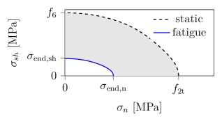
which represents a surface in stress-space when $f_{I}(\bm{\sigma})=1.0$ (see figure 5).

It should be emphesized that at the moment of crack insertion when equation 83 is satisfied, fatigue damage in the newly inserted cohesive crack segment is zero. Only after crack insertion, fatigue damage can accumulate according to the formulation presented in the previous section.

Figure 5: Fatigue and static damage initiation surfaces in stress-space

Shifted cohesive relation

Cohesive XFEM segments are inserted on the fly when the stress criterion is reached. The static initiation stress used in this work is the B-K interpolation of the elastic stored energy [53] before the peak at zero damage (see equation 80). For fatigue damage, the fatigue crack insertion criterion presented in the prevous section is used.

At the time of insertion, the stress in the material is non-zero. Therefore, following [54], Hille’s approach is used [55] where a shift is applied such that the traction for zero opening in the cohesive segment is in equilibrium with the stress in the bulk $\bm{\sigma}$ before and after insertion. The shift at the moment of crack insertion is computed as

$$\llbracket\textbf{u}\rrbracket_{\mathrm{shift}}=\textbf{K}^{-1}\bm{\sigma}\textbf{n}$$ (84)

The updated traction at current time $n$ is computed with equation 1 where the displacement jump is the sum of the jump passed to the integration point $\llbracket\textbf{u}\rrbracket_{\mathrm{FEM}}$ and the shift $\llbracket\textbf{u}\rrbracket_{\mathrm{shift}}$ (see figure 6).

Figure 6: Shifted fatigue cohesive zone model

2.2.   Adaptive cycle jumping

The cycle increment during fatigue loading is determined with a measure based on the number of global Newton-Raphson iterations $N_{\mathrm{iter}}$, following a strategy similar to [56] as previously applied in static loading [8]. The cycle increment $\Delta N$ for the next time step $n+1$ is computed from the current (converged) time step $n$ as

$$\Delta N^{(n+1)}=C^{-(\frac{n_{\mathrm{iter}}-n_{\mathrm{iter}}^{\mathrm{opt}}}{\xi})}\Delta N^{(n)}$$ (85)

where $C$, $\xi$ and $N_{\mathrm{iter}}^{\mathrm{opt}}$ are model parameters. If convergence is not reached within a specified maximum number of iterations $n_{\mathrm{iter}}^{\mathrm{max}}$, the step is cancelled and restarted with a reduced cycle increment $\Delta N^{(n)}\leftarrow c_{\mathrm{red}}\Delta N^{(n)}$.

3.   Examples

First a simple 1D case is simulated with a single XFEM element and shifted cohesive relation in order to verify the presented modeling approaches and to demonstrate the improved accuracy with the implicit fatigue damage update. As a second example, a DCB test is simulated where the importance of an implicit scheme for integrating the damage rate function is highlighted. In the last example, an open-hole [$\pm 45$]_s-laminate simulation is shown to demonstrate the capabilities of the numerical framework in simulating the complex interaction of matrix cracking and interface delamination under fatigue loading.

3.1.   Example A: Single XFEM cohesive element test

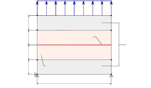
Firstly, a simple case under uniaxial tension is simulated (see figure 7). The maximum applied stress level is $\sigma^{\mathrm{\mathrm{max}}}=$6\text{\,}\mathrm{M}\mathrm{P}\mathrm{a}$$. The tensile strength, mode-I fracture energy and dummy stiffness are $f_{t}=$10\text{\,}\mathrm{M}\mathrm{P}\mathrm{a}$$, $G_{Ic}=0.1$ and $K=${10}^{4}\text{\,}\mathrm{N}\mathrm{/}\mathrm{m}\mathrm{m}$$. The fatigue model parameters are $p=\beta$, $\eta=0.8$ and $\epsilon=0.2$. The XFEM crack is inserted in the middle element when the applied stress $\sigma^{\mathrm{max}}=0.2f_{t}$.

For the case of constant tension, the damage evolution can be analytically derived as shown in [49]. The time to failure is given with the following equation

$$N_{\mathrm{fail}}=\bar{N}(\sigma^{\mathrm{max}})=\gamma E^{\beta}\Big{(}\frac{\sigma^{\mathrm{max}}}{f_{t}}\Big{)}^{-\beta}\Big{[}1-\Big{(}\frac{\sigma^{\mathrm{max}}}{f_{t}}\Big{)}^{p+1}\Big{]}$$ (86)

where $\gamma=10^{7}$ (see equation 22).

In the case of the maximum stress level considered in this example, the damage state at which the material point is considered to have failed is equal to $\mathcal{D}_{\mathrm{fail}}=1-\sigma^{\mathrm{max}}/f_{t}=0.4$.

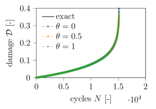
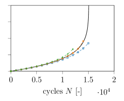
The damage evolution as a result of three different time integration parameter values $\theta\in\{0,0.5,1\}$ (see equation 27), corresponding to Euler forward, trapezoidal rule and Euler backward, is shown in figure 8. When the step size is sufficiently small, as in the case with $\Delta N=10$, all three methods show good correspondence with the exact analytical result. When the step size is increased to $\Delta N=1000$, the trapezoidal rule with $\theta=0.5$ results in the most accurate response as it is second-order accurate, while Euler forward and Euler backward underestimate and overestimate the damage accumulation, respectively. Also note that with $\Delta N=1000$, the final damage $\mathcal{D}_{\mathrm{fail}}=0.4$ is not reached. This is caused by the fact that in the constant stress simulation, no equilibrium solution exists when $\mathcal{D}>\mathcal{D}_{\mathrm{fail}}$.

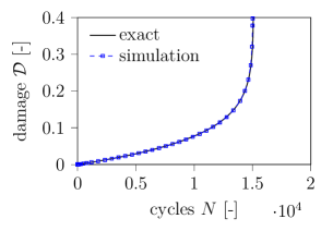
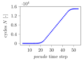
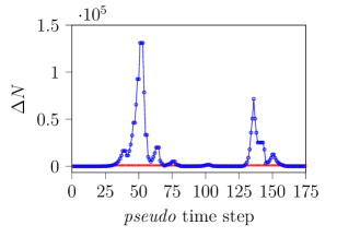
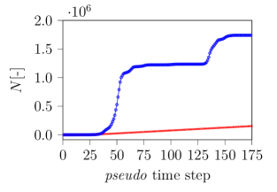
The simulations are also performed with the adaptive cycle jump scheme described in section 2.2, where the cycle increment size $\Delta N$ is chosen based on the convergence characteristics from the previous pseudo time step. The damage evolution is shown in fig. 9(a). The number of elapsed cycles in each pseudo time step as a result of the accumulation of the (adaptive) cycle increments is shown in fig. 9(b). It can be observed that the implicit damage update with adaptive stepping based on global convergence behavior is capable of tracing the full evolution of damage with high accuracy and efficient time stepping.

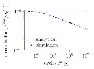
The exercise is repeated with four different stress levels. The corresponding number of cycles to failure is plotted on the underlying S-N curve that serves as input for the model in figure 10. A good match is obtained with the numerical simulations, which verifies the XFEM implementation with shifted cohesive relation and implicit fatigue damage update.

Figure 7: Specimen dimensions of single element test

(a)

(b)

Figure 8: Damage evolution with two different constant cycle increments $\Delta N$. (a) $\Delta N=10$, (b) $\Delta N=1000$

(a) adaptive $\Delta N$

(b) elapsed number of cycles in each pseudo time step

Figure 9: Damage evolution and elapsed cycles per pseudo time step with adaptive cycle increment $\Delta N$

Figure 10: Verification of the input at different stress levels

3.2.   Example B: Double cantilever beam test

The improved performance of the fatigue CZM in simulating fatigue crack growth in a DCB test is compared to the existing formulation in [37]. For this purpose, the case recently studied in [57] with optimal fatigue parameters is used for comparison. The results are compared with the experiments done by [58] [58]. The plies have height $h=$1.472\text{\,}\mathrm{m}\mathrm{m}$$, width $25\text{\,}\mathrm{m}\mathrm{m}$ and an initial crack length $a_{0}=$51.2\text{\,}\mathrm{m}\mathrm{m}$$. The computational model is shown in figure 11.

Figure 11: Computational model of the DCB specimen. The element width is $0.05\text{\,}\mathrm{m}\mathrm{m}$ in the refined zone (region in dark grey) and $0.25\text{\,}\mathrm{m}\mathrm{m}$ outside this zone (region in light brown). Eight elements are used across the thickness of each arm

Each arm of the DCB specimen is modeled with 2D plane strain linear quadrilateral elements with unit thickness. The bulk material is linearly elastic orthotropic and the static interface material properties and optimal fatigue model parameters determined in [57] are given in table 1. Furthermore, normal dummy stiffness $K_{n}=$2\text{\times}{10}^{5}\text{\,}\mathrm{N}\mathrm{/}\mathrm{m}\mathrm{m}$$ is used. In order to drive the fatigue cracking process, displacement control is used with a maximum applied displacement $u^{\mathrm{max}}_{\mathrm{p}}=$5\text{\,}\mathrm{mm}$$ and global load-ratio $R=0.1$.

Comparison integration schemes with constant cycle increments

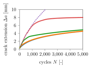
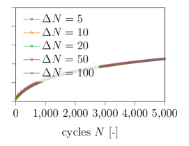
To compare the performance of the implicit damage update with the explicit update, constant cycle increments $\Delta N\in\{10,20,50,100\}$ are used. For the implicit scheme, the numerical time integration parameter is set to $\theta=0.5$, which reduces to the trapezoidal rule with second-order accuracy. Figure 12 shows the crack extension $\Delta a$ as a function of number of cycles $N$, which clearly indicates the strong influence of the step size for the explicit fatigue damage update, whereas with the implicit scheme, the global response is insensitive to the step size in the investigated range.

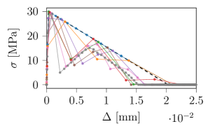
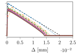
Figure 13 shows the traction-opening history of several integration points along the interface for the case with $\Delta N=50$. With the explicit scheme, numerically unstable damage growth can be observed which is fully removed with the implicit scheme where damage grows during fatigue loading in a continuous fashion. The effect of numerically unstable damage growth is most profound for integration points in the cohesive zone (for which $\mathcal{D}\in(0,1)$) after the static ramp-up phase, where a sharp drop in stiffness is observed for the first fatigue cycles (see figure 13).

Under displacement control, the energy release rate (ERR) reduces as the crack extends and the compliance increases. Since the ERR is closely related to the area under the traction-opening relation, points move farther away from the softening line, which in turn decreases the rate of fatigue damage accumulation $\mathrm{d}\mathcal{D}/\mathrm{d}N$ as described by the underlying S-N curve. Consequently, larger step sizes can be used as the crack propagates.

Simulations with adaptive cycle jumping

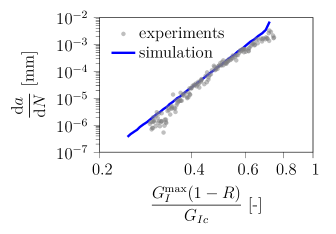
Under displacement control, the energy release rate (ERR) reduces and a sweep over several ERR values is performed in a single DCB simulation. Therefore, the crack growth rate can be computed as a function of the ERR at the maximum load level and compared to the response of the experimental Paris relation. The crack length $a$ is computed numerically and is based on the average damage along the interface following [46]:

$$a=a_{0}+\sum^{N_{\mathrm{ip}}}_{\mathrm{ip}=1}\mathcal{D}_{\mathrm{ip}}J_{\mathrm{ip}}w_{\mathrm{ip}}$$ (87)

where $J_{\mathrm{ip}}w_{\mathrm{ip}}$ is the product of the Jacobian and the integration weight. The crack growth rate at time step $n$ is then approximated with Euler backward differentiation:

$$\derivative{a}{N}^{(n)}\approx\frac{a^{(n)}-a^{(n-1)}}{\Delta N}$$ (88)

The ERR at maximum load $G^{\mathrm{max}}_{I}$ is computed according to the ASTM D5528 standard [59]

$$G^{\mathrm{max}}_{I}=\frac{3F^{\mathrm{max}}u^{\mathrm{max}}_{\mathrm{p}}}{2b(a+\Delta_{\mathrm{cor}})}$$ (89)

where $F^{\mathrm{max}}$ is the reaction force at the node where $u^{\mathrm{max}}_{\mathrm{p}}$ is applied (see figure 11), $b$ is the specimen width and $\Delta_{\mathrm{cor}}$ takes into account the effect of finite rotations (here $\Delta_{\mathrm{cor}}=$6.2\text{\,}\mathrm{m}\mathrm{m}$$). The computed crack growth rate vs ERR is shown in figure 15, from which it can be observed that a good match is obtained with the experimental results.

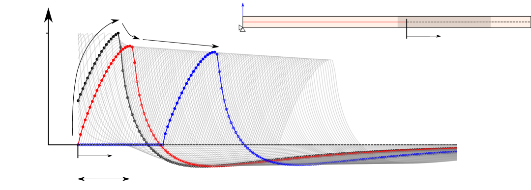
The complete evolution of the traction is shown in figure 14, from which three phases can be distinguished. First, the maximum load is applied quasi-statically. When the first load cycles are applied (shown in black), the fracture process continuous to develop into a complete cohesive zone during the onset phase (shown in red). When the process zone has fully developed, propagation of the crack takes place (shown in blue).

(a)

(b)

Figure 12: Crack extension with number of cycles as a result of (a) explicit and (b) implicit fatigue damage update

(a)

(b)

Figure 13: Traction-opening histories of several integration points along in the interface as a result of (a) explicit and (b) implicit fatigue damage update.

Figure 14: Traction profile evolution along the interface at different time steps shown in gray. The stages of the static ramp-up, fatigue crack onset and propagation are indicated with black, red and blue colors respectively.

Figure 15: Paris relation with simulation and with experimental results from [58]

Table 1: Ply material properties for the DCB specimen example. Taken from [57]

elastic constants ply		fracture properties interface		fatigue parameters
$E_{1}$	$154\text{\,}\mathrm{G}\mathrm{P}\mathrm{a}$	$f_{n}$	30 MPa	$\eta$	0.8757
$E_{2}=E_{3}$	8.5 GPa	$G_{Ic}$	$0.305\text{\,}\mathrm{N}\text{\,}{\mathrm{mm}}^{-1}$	$\epsilon$	0.2628
$G_{12}=G_{13}$	4.2 GPa			$p$	$\beta+0.915$
$\nu_{12}=\nu_{13}$	0.35
$\nu_{23}$	0.4

3.3.   Example C: Open-hole $[\pm 45]$-laminate

A $[\pm 45]$-laminate is simulated in order to demonstrate the capabilities of the developed fatigue failure framework to deal with progressive laminate failure. This case was previously studied in the context of static loading in [9] for the purpose of simulating the interaction between matrix cracking and delamination without fiber fracture.

Modeling preliminaries

The laminate has dimensions $$38\text{\,}\mathrm{m}\mathrm{m}$\times$16\text{\,}\mathrm{m}\mathrm{m}$\times$1\text{\,}\mathrm{m}\mathrm{m}$$ and contains a hole in the middle with a diameter of $6.4\text{\,}\mathrm{m}\mathrm{m}$. The plies have a thickness $t=$0.5\text{\,}\mathrm{mm}$$ and are modeled with plane stress XFEM elements, whereas delamination between the plies is modeled with zero-thickness interface elements. The constitutive relation of the matrix cohesive segments and interface integration points is described with the improved fatigue CZM presented in section 2.1. The material properties and the fatigue model parameters are given in table 2. The dummy stiffness of matrix cracks in normal direction is $K_{n}=$1.0\text{\times}{10}^{5}\text{\,}\mathrm{N}\text{\,}{\mathrm{mm}}^{-1}$$, whereas $K_{sh}$ is adapted according to equation 4. The shear stiffness of the interface is related to the shear modulus $G_{12}$ and thickness of the ply ($K_{d}=G_{12}/\frac{1}{2}t=$22\,000\text{\,}\mathrm{N}\mathrm{/}\mathrm{m}\mathrm{m}$$) according to [9], taking into account the effect of out-of-plane ply shear deformation. The computational domain is discretized using linear (constant strain) triangular elements with single-point Gauss integration. Upon crack insertion, a two-point Gauss scheme is employed in the XFEM crack segment. Three-point Newton-Cotes is used for the interface, following [9]. Furthermore, displacement control is used. The maximum applied displacement is $u^{\mathrm{max}}_{\mathrm{p}}=$0.1\text{\,}\mathrm{mm}$$ with global load ratio $R=0.1$.

Crack segments are inserted when the stress in the bulk integration point reaches the stress endurance limit (see section 2). The shift is applied in order to ensure traction continuity before and after insertion of the crack, which improves the convergence characteristics. At the end of a converged pseudo time step, a maximum of 100 segments can be inserted at a time. After insertion, the global Newton-Raphson loop is re-entered to equilibrate the solution with new crack segments [54]. With the XFEM representation, cracks can initiate at arbitrary locations within a predefined crack-spacing width $l_{\mathrm{c}}$.

Equation 85 is used to adapt the cycle increment $\Delta N$ throughout the simulations. The used stepping parameters are $C=2$, $\xi=2$, $n_{\mathrm{iter}}^{\mathrm{opt}}=4$, $n_{\mathrm{iter}}^{\mathrm{max}}=10$ and $c_{\mathrm{red}}=0.6$.

Table 2: Ply material properties for open-hole numerical example

elastic constants		fracture properties		fatigue parameters
$E_{1}$	$122.7\text{\,}\mathrm{G}\mathrm{P}\mathrm{a}$	$f_{2t}$	80 MPa	$\eta$	0.95
$E_{2}$	10.1 GPa	$f_{12}$	100 MPa	$\epsilon$	0.25
$G_{12}$	5.5 GPa	$G_{Ic}$	$0.969\text{\,}\mathrm{N}\text{\,}{\mathrm{mm}}^{-1}$	$p$	$\beta$
$\nu_{12}$	0.25	$G_{IIc}$	$1.719\text{\,}\mathrm{N}\text{\,}{\mathrm{mm}}^{-1}$
		$\eta$	2.284

Global response and damage development

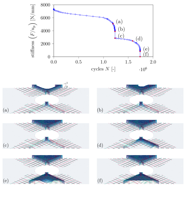
Simulations are performed with crack-spacing parameter $l_{c}=0.9$. The progressive nature of damage development is depicted in figure 16, which shows the reduction of global stiffness (reaction force over applied displacement at the end) as a function of cycle number $N$. At the indicated time instances, the damage profiles in the interface and the XFEM matrix cracks are shown. From these figures, several stages of damage development can be distinguished. Firstly, a gradual stiffness reduction takes place due to matrix cracking and delamination of the (small) triangular areas near the hole, followed by a rapid damage development (from (a) to (c)) due to combined matrix cracking and major delamination on one side of the hole. After this phase, a third stage of matrix cracking on the opposite side takes place (from (d) to (f)), leading to delamination with sharp stiffness drops until complete failure of the laminate. The deformed mesh is shown in figure 17, from which it can be observed that a transition from distributed to localized failure is obtained.

Time step dependence

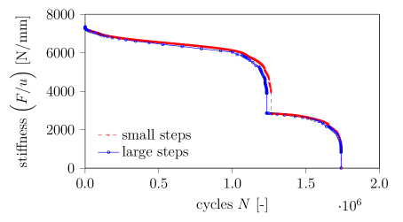
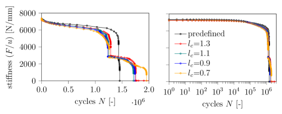
The influence of the adaptive cycle jumping scheme on the accuracy of the simulation is illustrated in figure 18, where the stiffness reduction is shown in fig. 18(a) with two different adaptive stepping parameters, corresponding to small and large cycle increments as depicted in fig. 18(c). For the small increment simulation, the maximum cycle jump is $\Delta N^{\mathrm{max}}=1000$. It can be observed that the progression of damage and the time to failure is only slightly affected by the large step sizes, thereby validating the choice to use global iterations as a measure for determining the cycle increment $\Delta N$ with implicit time integration of the fatigue damage rate function. Moreover, fig. 18(c) shows that the cycle jumping strategy with consistent tangent and implicit fatigue damage update allows a seamless transition through periods that require small steps and periods that allow for large cycle increments, with minimal influence on the accuracy.

Figure 16: Stiffness reduction as a function of number of cycles $N$ (top) and damage evolution at indicated time instances in interface (in blue) and XFEM matrix cracks in top ply (in red) and bottom ply (in green)

Figure 17: Deformations in the laminate showing a transition from distributed to localized failure

(a)

(b)

(c)

Figure 18: Influence of the cycle jump size. (a) stiffness reduction with two different cycle jump parameters corresponding to small and large step sizes. (b) cycle increments per pseudo time step. (c) accumulation of fatigue cycles throughout the simulation steps. The simulation with the small step strategy required more than 1500 time steps, whereas with the larger step sizes the simulation finished in 174 time steps

Crack-spacing parameter dependence

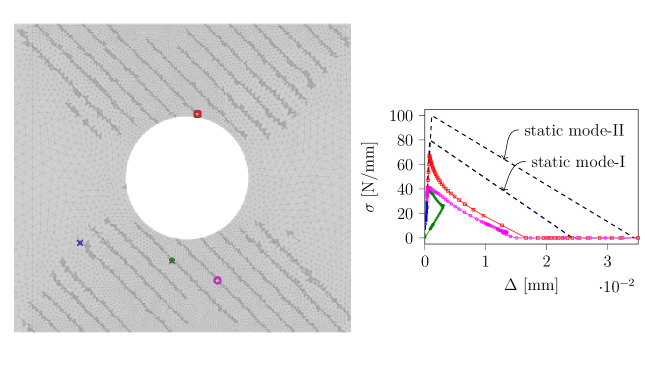
The exercise is repeated for several crack-spacing parameter values $l_{c}(\mathrm{mm})\in\{0.7,0.9,1.1,1.3\}$. Moreover, a case with two cracks per ply at predefined locations is included. The cracks are inserted in each ply in the direction of the fibers and tangential to the hole. The global stiffness reduction is shown in figure 19. An interesting observation is that allowing more than two cracks per ply has a significant positive effect on the fatigue life of the considered laminate. This can be explained by the fact that matrix cracking results in a reduction of stress concentrations in the interface and thus less fatigue damage accumulation. Another observation is that the response varies slightly with different crack-spacing parameter values. However, the discrepancy is not monotonic, in the sense that reducing the spacing does not always lead to an increase in fatigue life. In fact, the difference can be explained by analysing figure 20, which depicts the damage in the XFEM matrix cracks in the bottom ply for each spacing parameter value $l_{\mathrm{c}}$. It can be observed that the crack density and patterns are different, which explains a different progression of stiffness reduction as observed in figure 19. However, when the response is shown on a log-scale, as is common practice with fatigue analysis, the difference vanishes.

Figure 21 shows the response in four integration points for the case of a crack spacing parameter $l_{c}=$0.9\text{\,}\mathrm{m}\mathrm{m}$$. As it can be observed, two of the selected points completely separate, while the other integration points unload. This indicates that not necessarily all XFEM cracks that have been inserted accumulate damage until complete material point failure, thereby allowing for simulating the transition from distributed damage to localized failure. Another interesting fact is that the traction-separation response is not parallel to the static softening line, as is the case with the simulated DCB case in the previous section (cf. fig. 13(b)), indicating the accurate time integration of the damage evolution equation.

Figure 19: Influence of the spacing parameter $l_{\mathrm{c}}$ on the simulation results on two different scales: linear on the left and log-scale on the right.

Figure 20: Final damage $\mathcal{D}$ in XFEM cracks in bottom ply (shown in green) for different crack spacing parameter values $l_{\mathrm{c}}$. The delaminated area in the interface is shown in dark gray

Figure 21: Traction-opening histories (right) of four XFEM integration points at different crack locations in the ply (left)

4.   Conclusion

A numerical framework for simulating progressive fatigue failure has been presented in this paper. The recently proposed fatigue cohesive zone model by [37], which covers initiation and propagation, has been improved with an implicit time integration scheme and consistent linearization of both the underlying quasi-static and the fatigue cohesive relation. Furthermore, the fatigue cohesive zone model has been combined with XFEM for modeling mesh-independent transverse matrix cracks in full-laminate analyses.

It has been shown with numerical examples that the improved damage update results in more accurate and efficient analyses. The capabilities of the numerical framework have been demonstrated with the simulation of an open-hole [$\pm 45$]-laminate under fatigue loading. The numerical model can accurately simulate the interaction of transverse matrix cracking and delamination. A slight sensitivity to the numerical crack-spacing parameter has been observed, although within acceptable range for predicting fatigue life.

References

- [1] Michael R. Wisnom and Stephen R. Hallett “The Role of Delamination in Strength, Failure Mechanism and Hole Size Effect in Open Hole Tensile Tests on Quasi-Isotropic Laminates” In Composites Part A: Applied Science and Manufacturing 40.4 Elsevier Ltd, 2009, pp. 335–342 DOI: 10.1016/j.compositesa.2008.12.013
- [2] B.. Green, M.. Wisnom and S.. Hallett “An Experimental Investigation into the Tensile Strength Scaling of Notched Composites” In Composites Part A: Applied Science and Manufacturing 38.3, 2007, pp. 867–878 DOI: 10.1016/j.compositesa.2006.07.008
- [3] O.. Nixon-Pearson, S.. Hallett, P.. Withers and J. Rouse “Damage Development in Open-Hole Composite Specimens in Fatigue. Part 1: Experimental Investigation” In Composite Structures 106 Elsevier Ltd, 2013, pp. 882–889 DOI: 10.1016/j.compstruct.2013.05.033
- [4] F Aymerich and M.. Found “Response of Notched Carbon/PEEK and Carbon/Epoxy Laminates Subjected to Tension Fatigue Loading” In Fatigue and Fracture of Engineering Materials and Structures 23.8, 2000, pp. 675–683 DOI: 10.1046/j.1460-2695.2000.00262.x
- [5] Bilel Aidi, Michael K. Philen and Scott W. Case “Progressive Damage Assessment of Centrally Notched Composite Specimens in Fatigue” In Composites Part A: Applied Science and Manufacturing 74 Elsevier Ltd, 2015, pp. 47–59 DOI: 10.1016/j.compositesa.2015.03.022
- [6] Wen Guang Jiang, Stephen R. Hallett, Ben G. Green and Michael R. Wisnom “A Concise Interface Constitutive Law for Analysis of Delamination and Splitting in Composite Materials and Its Application to Scaled Notched Tensile Specimens” In International Journal for Numerical Methods in Engineering 69.9, 2007, pp. 1982–1995 DOI: 10.1002/nme.1842
- [7] S.. Hallett, B.. Green, W.. Jiang and M.. Wisnom “An Experimental and Numerical Investigation into the Damage Mechanisms in Notched Composites” In Composites Part A: Applied Science and Manufacturing 40.5 Elsevier Ltd, 2009, pp. 613–624 DOI: 10.1016/j.compositesa.2009.02.021
- [8] F.. Meer and L.. Sluys “A Phantom Node Formulation with Mixed Mode Cohesive Law for Splitting in Laminates” In International Journal of Fracture 158.2, 2009, pp. 107–124 DOI: 10.1007/s10704-009-9344-5
- [9] F.. Van der Meer and L.. Sluys “Mesh-Independent Modeling of Both Distributed and Discrete Matrix Cracking in Interaction with Delamination in Composites” In Engineering Fracture Mechanics 77.4, 2010, pp. 719–735 DOI: 10.1016/j.engfracmech.2009.11.010
- [10] Anita Hansbo and Peter Hansbo “A Finite Element Method for the Simulation of Strong and Weak Discontinuities in Solid Mechanics” In Computer Methods in Applied Mechanics and Engineering 193.33-35, 2004, pp. 3523–3540 DOI: 10.1016/j.cma.2003.12.041
- [11] B.. Chen, T.. Tay, S.. Pinho and V..C. Tan “Modelling the Tensile Failure of Composites with the Floating Node Method” In Computer Methods in Applied Mechanics and Engineering 308 Elsevier B.V., 2016, pp. 414–442 DOI: 10.1016/j.cma.2016.05.027
- [12] B.Y. Chen, S.T. Pinho, N.V. De Carvalho, P.M. Baiz and T.E. Tay “A Floating Node Method for the Modelling of Discontinuities in Composites” In Engineering Fracture Mechanics 127, 2014, pp. 104–134 DOI: 10.1016/j.engfracmech.2014.05.018
- [13] Michael J Swindeman, Endel V Iarve, Robert A Brockman, David H Mollenhauer and Stephen R Hallett “Strength Prediction in Open Hole Composite Laminates by Using Discrete Damage Modeling” In AIAA Journal 51.4, 2013, pp. 936–945 DOI: 10.2514/1.J051773
- [14] B.. Chen, T.. Tay, P.. Baiz and S.. Pinho “Numerical Analysis of Size Effects on Open-Hole Tensile Composite Laminates” In Composites Part A: Applied Science and Manufacturing 47.1, 2013, pp. 52–62 DOI: 10.1016/j.compositesa.2012.12.001
- [15] Victor Achard, Christophe Bouvet, Bruno Castanié and Clément Chirol “Discrete Ply Modelling of Open Hole Tensile Tests” In Composite Structures 113.1 Elsevier Ltd, 2014, pp. 369–381 DOI: 10.1016/j.compstruct.2014.03.031
- [16] Luiz F Kawashita, Alexandre Bedos and Stephen R Hallett “Modelling Mesh Independent Transverse Cracks in Laminated Composites with a Simplified Cohesive Segment Method” In Computers, Materials and Continua 32.2, 2012, pp. 133–158
- [17] Endel V Iarve, Kevin Hoos, Michael Braginsky, Eric Zhou and David H Mollenhauer “Progressive Failure Simulation in Laminated Composites under Fatigue Loading by Using Discrete Damage Modeling” In Journal of Composite Materials 51.15, 2016, pp. 2143–2161 DOI: 10.1177/0021998316681831
- [18] Zhaoyang Ma, Jianlin Chen, Qingda Yang, Zheng Li and Xianyue Su “Progressive Fracture Analysis of the Open-Hole Composite Laminates: Experiment and Simulation” In Composite Structures 262 Elsevier Ltd, 2021, pp. 113628 DOI: 10.1016/j.compstruct.2021.113628
- [19] O. Falcó, R.. Ávila, B. Tijs and C.. Lopes “Modelling and Simulation Methodology for Unidirectional Composite Laminates in a Virtual Test Lab Framework” In Composite Structures 190 Elsevier Ltd, 2018, pp. 137–159 DOI: 10.1016/j.compstruct.2018.02.016
- [20] M.. Le, H. Bainier, D. Néron, C. Ha-Minh and P. Ladevèze “On Matrix Cracking and Splits Modeling in Laminated Composites” In Composites Part A: Applied Science and Manufacturing 115 Elsevier Ltd, 2018, pp. 294–301 DOI: 10.1016/j.compositesa.2018.10.002
- [21] Jing Fen Chen, Evgeny V. Morozov and Krishnakumar Shankar “Simulating Progressive Failure of Composite Laminates Including In-Ply and Delamination Damage Effects” In Composites Part A: Applied Science and Manufacturing 61 Elsevier Ltd, 2014, pp. 185–200 DOI: 10.1016/j.compositesa.2014.02.013
- [22] Chen Wang and Chao Zhang “Discussions on Extension of Traditional Cohesive Element for Delamination Modeling of Laminates Used in Combination with Phantom Node Intraply Elements” In Composite Structures 261 Elsevier Ltd, 2021, pp. 113588 DOI: 10.1016/j.compstruct.2021.113588
- [23] O.. Nixon-Pearson, S.. Hallett, P.. Harper and L.. Kawashita “Damage Development in Open-Hole Composite Specimens in Fatigue. Part 2: Numerical Modelling” In Composite Structures 106, 2013, pp. 890–898 DOI: 10.1016/j.compstruct.2013.05.019
- [24] Paul W. Harper and Stephen R. Hallett “A Fatigue Degradation Law for Cohesive Interface Elements – Development and Application to Composite Materials” In International Journal of Fatigue 32.11 Elsevier Ltd, 2010, pp. 1774–1787 DOI: 10.1016/j.ijfatigue.2010.04.006
- [25] Luiz F. Kawashita and Stephen R. Hallett “A Crack Tip Tracking Algorithm for Cohesive Interface Element Analysis of Fatigue Delamination Propagation in Composite Materials” In International Journal of Solids and Structures 49.21, 2012, pp. 2898–2913 DOI: 10.1016/j.ijsolstr.2012.03.034
- [26] Wei-Tsen Lu, Zhenjia Gao, Hari K. Adluru, Kevin H. Hoos, Waruna P. Seneviratne, David H. Mollenhauer and Endel V. Iarve “Fatigue Damage Modeling in Laminated Composite by Using Rx-FEM and Strength Tracking Method” In Composites Part A: Applied Science and Manufacturing 163, 2022, pp. 107199 DOI: 10.1016/j.compositesa.2022.107199
- [27] Chongcong Tao, Supratik Mukhopadhyay, Bing Zhang, Luiz F. Kawashita, Jinhao Qiu and Stephen R. Hallett “An Improved Delamination Fatigue Cohesive Interface Model for Complex Three-Dimensional Multi-Interface Cases” In Composites Part A: Applied Science and Manufacturing 107, 2018, pp. 633–646 DOI: 10.1016/j.compositesa.2018.02.008
- [28] J. Llobet, P. Maimí, A. Turon, B.L.V. Bak, E. Lindgaard, L. Carreras, Y. Essa and F. Martin de la Escalera “A Continuum Damage Model for Composite Laminates: Part IV- Experimental and Numerical Tests” In Mechanics of Materials 154, 2021, pp. 103686 DOI: 10.1016/j.mechmat.2020.103686
- [29] Chongcong Tao, Chao Zhang, Hongli Ji and Jinhao Qiu “A Paris-law-informed Neural Fatigue Cohesive Model and Its Application to Open-Hole Composite Laminates” In International Journal of Solids and Structures 267, 2023, pp. 112158 DOI: 10.1016/j.ijsolstr.2023.112158
- [30] P.C. Paris, M.P. Gomes and W.E. Anderson “A Rational Analytic Theory of Fatigue” In Trend Engineering 388, 1961
- [31] B.L.V Bak, A. Turon, A. Lindgaard and E. Lund “A Simulation Method for High-Cycle Fatigue-Driven Delamination Using a Cohesive Zone Model” In International Journal for Numerical Methods in Engineering, 2016 DOI: 10.1002/nme.5117 A
- [32] M. Latifi, F.P.. Meer and L.J.. Sluys “A Level Set Model for Simulating Fatigue-Driven Delamination in Composites” In International Journal of Fatigue 80 Elsevier Ltd, 2015, pp. 434–442 DOI: 10.1016/j.ijfatigue.2015.07.003
- [33] A. Turon, J. Costa, P.P. Camanho and C.G. Dávila “Simulation of Delamination in Composites under High-Cycle Fatigue” In Composites Part A: Applied Science and Manufacturing 38.11, 2007, pp. 2270–2282 DOI: 10.1016/j.compositesa.2006.11.009
- [34] L. Carreras, A. Turon, B.L.V..V. Bak, E. Lindgaard, J. Renart, F. Martin de la Escalera and Y. Essa “A Simulation Method for Fatigue-Driven Delamination in Layered Structures Involving Non-Negligible Fracture Process Zones and Arbitrarily Shaped Crack Fronts” In Composites Part A: Applied Science and Manufacturing 122 Elsevier Ltd, 2019, pp. 107–119 DOI: 10.1016/j.compositesa.2019.04.026
- [35] Ahmad Amiri-Rad and Mohammad Mashayekhi “A Cohesive Zone Approach for Fatigue-Driven Delamination Analysis in Composite Materials” In Applied Composite Materials 24.4 Applied Composite Materials, 2017, pp. 751–769 DOI: 10.1007/s10443-016-9543-y
- [36] Ahmad Amiri-Rad, Mohammad Mashayekhi and Frans P. Meer “Cohesive Zone and Level Set Method for Simulation of High Cycle Fatigue Delamination in Composite Materials” In Composite Structures 160, 2017, pp. 61–69 DOI: 10.1016/j.compstruct.2016.10.041
- [37] Carlos G. Dávila “From S-N to the Paris Law with a New Mixed-Mode Cohesive Fatigue Model for Delamination in Composites” In Theoretical and Applied Fracture Mechanics 106, 2020, pp. 102499 DOI: 10.1016/j.tafmec.2020.102499
- [38] Michael May and Stephen R. Hallett “A Combined Model for Initiation and Propagation of Damage under Fatigue Loading for Cohesive Interface Elements” In Composites Part A: Applied Science and Manufacturing 41.12, 2010, pp. 1787–1796 DOI: 10.1016/j.compositesa.2010.08.015
- [39] Michael May, Rhys Pullin, Mark Eaton, Carol Featherston and Stephen R. Hallett “An Advanced Model for Initiation and Propagation of Damage under Fatigue Loading - Part II: Matrix Cracking Validation Cases” In Composite Structures 93.9 Elsevier Ltd, 2011, pp. 2350–2357 DOI: 10.1016/j.compstruct.2011.03.023
- [40] S. Nojavan, D. Schesser and Q.. Yang “An in Situ Fatigue-CZM for Unified Crack Initiation and Propagation in Composites under Cyclic Loading” In Composite Structures 146 Elsevier Ltd, 2016, pp. 34–49 DOI: 10.1016/j.compstruct.2016.02.060
- [41] A. Turon, P.. Camanho, J. Costa and C.. Dávila “A Damage Model for the Simulation of Delamination in Advanced Composites under Variable-Mode Loading” In Mechanics of Materials 38.11, 2006, pp. 1072–1089 DOI: 10.1016/j.mechmat.2005.10.003
- [42] A. Turon, E.. González, C. Sarrado, G. Guillamet and P. Maimí “Accurate Simulation of Delamination under Mixed-Mode Loading Using a Cohesive Model with a Mode-Dependent Penalty Stiffness” In Composite Structures 184 Elsevier, 2018, pp. 506–511 DOI: 10.1016/j.compstruct.2017.10.017
- [43] Giuliano Allegri “A Unified Formulation for Fatigue Crack Onset and Growth via Cohesive Zone Modelling” In Journal of the Mechanics and Physics of Solids 138 Elsevier Ltd, 2020, pp. 103900 DOI: 10.1016/j.jmps.2020.103900
- [44] Antonio Raimondo, Carlos G. Dávila and Chiara Bisagni “Cohesive Analysis of a 3D Benchmark for Delamination Growth under Quasi-static and Fatigue Loading Conditions” In Fatigue and Fracture of Engineering Materials and Structures, 2022 DOI: 10.1111/FFE.13712
- [45] L. Carreras, J. Renart, A. Turon, J. Costa, B..V. Bak, E. Lindgaard, F. Martin de la Escalera and Y. Essa “A Benchmark Test for Validating 3D Simulation Methods for Delamination Growth under Quasi-Static and Fatigue Loading” In Composite Structures 210 Elsevier Ltd, 2019, pp. 932–941 DOI: 10.1016/j.compstruct.2018.12.008
- [46] Mathew W. Joosten, Carlos G. Dávila and Qingda Yang “Predicting Fatigue Damage in Composites Subjected to General Loading Conditions” In Composites Part A: Applied Science and Manufacturing 156, 2022, pp. 106862 DOI: 10.1016/j.compositesa.2022.106862
- [47] Yu Jui Liang, Carlos G. Dávila and Endel V. Iarve “A Reduced-Input Cohesive Zone Model with Regularized Extended Finite Element Method for Fatigue Analysis of Laminated Composites in Abaqus” In Composite Structures 275 Elsevier Ltd, 2021, pp. 114494 DOI: 10.1016/j.compstruct.2021.114494
- [48] I. Leciñana, J. Renart, A. Turon, J. Zurbitu and B.H.A.H. Tijs “Characterization and Analysis of the Mode I Interlaminar Fatigue Behaviour of Thermoplastic Composites Considering R -Curve Effects” In Engineering Fracture Mechanics, 2023, pp. 109273 DOI: 10.1016/j.engfracmech.2023.109273
- [49] Carlos G Dávila, Cheryl A Rose, Gretchen B Murri, Wade C Jackson and William M Johnston “Evaluation of Fatigue Damage Accumulation Functions for Delamination Initiation and Propagation” In Nasa/Tp–2020-220584, 2020
- [50] M L Benzeggagh and M Kenane “Measurement of Mixed-Mode Delamination Fracture Toughness of Uniderictional Glass/Epoxy Composites with Mixed-Mode Bending” In Composites Science and Technology 56, 1996, pp. 439–449 DOI: 10.1016/0266-3538(96)00005-X
- [51] A. Turon, P.. Camanho, J. Costa and J. Renart “Accurate Simulation of Delamination Growth under Mixed-Mode Loading Using Cohesive Elements: Definition of Interlaminar Strengths and Elastic Stiffness” In Composite Structures 92.8 Elsevier Ltd, 2010, pp. 1857–1864 DOI: 10.1016/j.compstruct.2010.01.012
- [52] Robert C. Juvinall and Kurt M. Marshek “Fundamentals of Machine Component Design” Hoboken, NJ: John Wiley & Sons, 2012
- [53] E.. González, P. Maimí, A. Turon, P.. Camanho and J. Renart “Simulation of Delamination by Means of Cohesive Elements Using an Explicit Finite Element Code” In Computers, Materials and Continua 9.1, 2009, pp. 51–92
- [54] Frans P. Van der Meer “Mesolevel Modeling of Failure in Composite Laminates: Constitutive, Kinematic and Algorithmic Aspects” In Archives of Computational Methods in Engineering 19.3, 2012, pp. 381–425 DOI: 10.1007/s11831-012-9076-y
- [55] T.. Hille, A..J. Suiker and S. Turteltaub “Microcrack Nucleation in Thermal Barrier Coating Systems” In Engineering Fracture Mechanics 76.6 Elsevier Ltd, 2009, pp. 813–825 DOI: 10.1016/j.engfracmech.2008.12.010
- [56] Clemens V. Verhoosel, Joris J.. Remmers and Miguel A. Gutiérrez “A Dissipation-Based Arc-Length Method for Robust Simulation of Brittle and Ductile Failure” In International Journal for Numerical Methods in Engineering 77.9, 2009, pp. 1290–1321 DOI: 10.1002/nme.2447
- [57] I. Leciñana, J. Zurbitu, J. Renart and A. Turon “A Robust Fatigue Parameter Determination Method for a Local Fatigue Cohesive Zone Model” In International Journal of Fatigue, 2023, pp. 107582 DOI: 10.1016/j.ijfatigue.2023.107582
- [58] J. Renart, S. Budhe, L. Carreras, J.A. Mayugo and J. Costa “A New Testing Device to Simultaneously Measure the Mode I Fatigue Delamination Behavior of a Batch of Specimens” In International Journal of Fatigue 116, 2018, pp. 275–283 DOI: 10.1016/j.ijfatigue.2018.06.021
- [59] “ASTM D5528-01, Standard Test Method for Mode I Interlaminar Fracture Toughness of Unidirectional Fiber-Reinforced Polymer Matrix Composites Annual Book of ASTM Standards, American Society for Testing and Materials 2002.” In Book of ASTM Standards, American Society for Testing and Materials, West Conshohocken, PA, 2002