Deep learning probability flows and entropy production rates in active matter

Abstract

Active matter systems, from self-propelled colloids to motile bacteria, are characterized by the conversion of free energy into useful work at the microscopic scale. These systems generically involve physics beyond the reach of equilibrium statistical mechanics, and a persistent challenge has been to understand the nature of their nonequilibrium states. The entropy production rate and the magnitude of the steady-state probability current provide quantitative ways to do so by measuring the breakdown of time-reversal symmetry and the strength of nonequilibrium transport of measure. Yet, their efficient computation has remained elusive, as they depend on the system’s unknown and high-dimensional probability density. Here, building upon recent advances in generative modeling, we develop a deep learning framework that estimates the score of this density. We show that the score, together with the microscopic equations of motion, gives direct access to the entropy production rate, the probability current, and their decomposition into local contributions from individual particles, spatial regions, and degrees of freedom. To represent the score, we introduce a novel, spatially-local transformer-based network architecture that learns high-order interactions between particles while respecting their underlying permutation symmetry. We demonstrate the broad utility and scalability of the method by applying it to several high-dimensional systems of interacting active particles undergoing motility-induced phase separation (MIPS). We show that a single instance of our network trained on a system of 4096 particles at one packing fraction can generalize to other regions of the phase diagram, including systems with as many as 32768 particles. We use this observation to quantify the spatial structure of the departure from equilibrium in MIPS as a function of the number of particles and the packing fraction.

1 Introduction

Active matter systems are driven out of equilibrium by a continuous injection of energy at the microscopic scale of the constituent particles [1, 2, 3]. The nonequilibrium nature of their dynamics manifests itself in the breakdown of time-reversal symmetry (TRS), which can be quantified by the global rate of entropy production (EPR) [4, 5, 6, 7], and by the presence of probability currents at statistical steady state [8, 9, 10]. Despite their wide recognition as quantities of fundamental importance, computing either the global EPR or the magnitude of the probability current has remained a long-standing challenge. At a fundamental level, both are defined via the microscopic density for the system [11, 12], which is generically unknown outside of a few simplistic cases due to its high-dimensionality and its complexity [13].

The global EPR can in principle be computed directly from the microscopic equations of motion [14, 15, 16, 17, 18] by making use of the Crooks fluctuation theorem [19]. However, this leads to a single number, which fails to quantify where TRS breaks down spatially in the system, and fails to reveal which particles are responsible. This issue can be addressed for active matter field theories, where a similar approach leads to a local, spatially-dependent definition of the EPR [20, 21], but only after a coarse-graining of the microscopic dynamics. In general, methods based on the Crooks fluctuation theorem require a suitable definition of a time-reversed dyamics, which has been debated in the literature [22, 23, 24]. The use of a time reversal can be avoided via the stochastic thermodynamics definition of the entropy [11, 7], but doing so requires the logarithm of the system’s microscopic density, which is unavailable outside of the simplest cases. An orthogonal approach makes use of data compression algorithms to compute the global [25] or local EPR [26], but these methods are only valid asymptotically in the limit of infinite system size, and it is difficult to understand what they compute away from this limit. Several methods have also been developed to infer a global measure of the probability current [27, 28, 29], but thus far have been restricted to low-dimensional systems. For a detailed coverage on the use of the EPR and steady-state currents to quantify nonequilibrium effects in active matter, we refer the reader to [2].

Here, building upon recent advances in generative modeling [30, 31, 32, 33, 34], we tackle the challenging problem of estimating spatially-local probability currents and entropy production rates directly from their microscopic definitions. To this end, we develop a machine learning method that estimates the gradient of the logarithm of the system’s probability density, which can be characterized as a solution to the many-body stationary Fokker-Planck equation (FPE). This quantity, known as the score function [30, 31], enters the definition of both the probability current and the EPR. We show how the method naturally decomposes the global EPR or probability current into microscopic contributions from the individual particles and their degrees of freedom, which enables us to identify spatial structure in the breakdown of TRS. To validate the accuracy of the learned solution, we develop diagnostics based on invariants of the stationary FPE that can be verified a-posteriori.

We apply the method to several model systems involving active swimmers: two swimmers on the torus, where we can visualize the EPR and the probability flow across the entire phase space, a system of $64$ swimmers in a harmonic trap, and a system of $4096$ swimmers undergoing motility-induced phase separation (MIPS) [35]. For the MIPS system, we learn using a novel spatially-local architecture that does not depend on the total number of swimmers, and we show that it can be extended to systems of up to $32,768$ swimmers at values of the packing fraction that differ from those seen during training. Despite the high-dimensionality of these latter examples, our approach provides us with a microscopic description of both the current and the local EPR. Importantly, this enables us to visualize the contributions of the individual particles directly without any need for averaging. We use this property to confirm theoretical predictions about the spatial features of entropy production in MIPS, such as concentration on the interface between the dilute and condensed phases [20, 26]. Our main contributions can be summarized as:

1. We revisit the framework of stochastic thermodynamics and show how signatures of nonequilibrium behavior and lack of time-reversibility, such as the probability current and the EPR, can be related to the score of the system’s stationary probability density.

2. We show how to use machine learning tools from the field of generative modeling to estimate the score function from microscopic data (Figure 1). To approximate this high-dimensional function accurately, we develop a new transformer neural network architecture that incorporates spatial locality and permutation symmetry. This enables transferability to systems with differing numbers of particles or packing fractions than seen at training.

3. We illustrate the usefulness of the approach on systems involving active particles undergoing MIPS, where we show that the method can quantify the EPR at the individual particle level as a function of the activity, number of particles, or packing fraction. We confirm that entropy is dominantly produced at the interface between the cluster and the gas.

These contributions continue in a line of work that seeks to apply methods based on machine learning to high-dimensional problems in scientific computing [36, 37, 38, 39, 40], applied mathematics [41, 34, 42, 43, 44, 45, 46, 47, 48, 49], and the physical sciences [50, 51, 52, 53, 54]. In particular, considerable research effort has been spent designing machine learning methods to compute solutions of the many-body Schrödinger equation [55, 56, 57, 58]; our work can be seen as an extension of this research effort to classical statistical mechanics and stochastic thermodynamics.

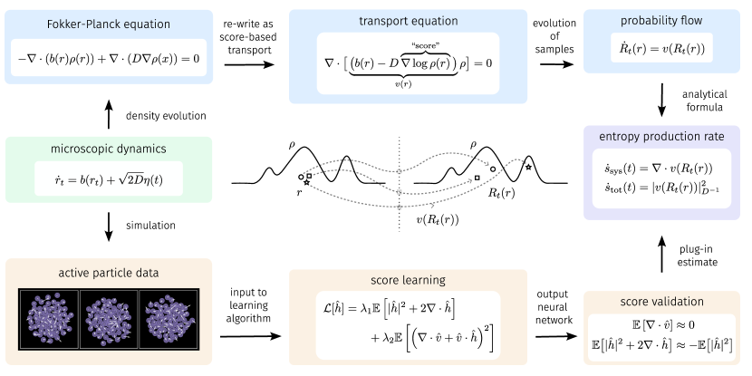
Figure 1: Method overview. (Green) The starting point for our approach is a microscopic dynamics describing the evolution of a set of interacting active particles. (Purple) The target is estimation of several definitions of the entropy production rate of the system, which we will accomplish by means of the probability flow. (Blue) Mathematically, our approach is built on viewing the system from the perspective of dynamical transport of measure. The microscopic stochastic dynamics induces a Fokker-Planck equation for a high-dimensional density describing the configuration of the system. This Fokker-Planck equation is equivalent to a transport equation that depends on the unknown “score” $\nabla\log\rho$ of the solution. The characteristics of this equation obey a probability flow ordinary differential equation, which gives immediate access to the entropy production rate. (Center) Illustration of nonequilibrium transport of measure at stationarity. (Orange) Algorithmically, our method approximates the unknown score by machine learning over a dataset of microscopic particle data. The learned approximation can be validated a-posteriori by checking invariants of the stationary Fokker-Planck equation, and can be plugged in directly to the definition of the entropy production rate to obtain an estimate.

2 Stochastic thermodynamics

\begin{overpic}[width=433.62pt]{figures/lowd/sde_trajs_and_density.pdf} \put(3.0,36.0){{A}} \put(51.0,36.0){{B}} \end{overpic}

\begin{overpic}[width=433.62pt]{figures/lowd/phase_portrait_and_current.pdf} \put(3.0,35.5){{C}} \put(51.0,35.5){{D}} \end{overpic}

Figure 2: Stochastic dynamics and probability flows. (A) Individual stochastic trajectories of (1) for $N=2$ and $d=1$ in the variables $x_{t}=x^{2}_{t}-x^{1}_{t}$ and $g_{t}=g^{2}_{t}-g^{1}_{t}$, with periodic boundary conditions on $[0,L]$. The trajectories $(x_{t},g_{t})$ tend to accumulate in two clusters corresponding to situations where particle 1 is just in front of particle 2 or vice-versa. This occurs because one particle catches up to the other in a typical trajectory (since either $|g_{t}^{1}|>|g_{t}^{2}|$ or $|g_{t}^{1}|<|g_{t}^{2}|$), but does not pass over it due to the short-range repulsive force between them. Random transitions between these modes occur when the magnitudes of $|g_{t}^{1}|$ and $|g_{t}^{2}|$ change order. (B) Stationary probability density function $\rho$ of $(x_{t},g_{t})$ confirming the metastability observed in (A): $\rho$ is the solution of the stationary FPE (3). (C) Visualization of the (diffusion-weighted) norm of the probability current $j$, defined in (4), over the phase space. The current is concentrated in the two modes, but is also nonzero along transition pathways between them. (D) Phase portrait of the probability flow (7). Similar to the stochastic trajectories in (A), the flow lines preserve the density $\rho$ in (B), but are deterministic and interpretable, highlighting limit cycles within and between the two clusters. A movie of these limit cycles in a frame with one particle fixed is available at this link.

2.1 Active swimmers

As an application of our approach, we will consider a suspension of $N$ self-propelled particles in $d=1$ or $d=2$ dimensions with translational degrees of freedom $x_{t}^{i}\in\mathbb{R}^{d}$ and orientational degrees of freedom $g_{t}^{i}\in\mathbb{R}^{d}$. Their dynamics is given by the so-called active Ornstein-Uhlenbeck, or Gaussian colored-noise model [59, 60, 61, 62, 15, 23]:

$$\dot{x}_{t}^{i} =-\mu\sum_{j\not=i}f(x_{t}^{i}-x_{t}^{j})+v_{0}g_{t}^{i}+\sqrt{2\epsilon}\,\eta_{x}^{i}(t),$$ (1)

$$\dot{g}_{t}^{i} =-\gamma g_{t}^{i}+\sqrt{2\gamma}\,\eta_{g}^{i}(t).$$

In (1), $\mu$ is the mobility, $f(x)$ is a short-range repulsive potential force whose specific form will be specified later, and $v_{0}\geq 0$ is the self-propulsion speed of the particles. $\eta^{i}_{x}(t)$ and $\eta^{i}_{g}(t)$ are independent white-noise sources, i.e., Gaussian processes with mean zero and covariances given by $\langle\eta_{x}^{i}(t)\eta_{x}^{j}(t^{\prime})\rangle=\langle\eta_{g}^{i}(t)\eta_{g}^{j}(t^{\prime})\rangle=\delta(t-t^{\prime})\delta_{i,j}Id$. $\epsilon\geq 0$ sets the scale of the thermal noise, while $\gamma>0$ tunes the persistence timescale of the self-propulsion. The orientational degrees of freedom $g_{t}^{i}$ introduce an active noise term with a finite correlation time $1/\gamma$ into the translational dynamics for $r_{t}^{i}$; the presence of this correlated noise drives the system out of equilibrium for any $v_{0}\not=0$ and $\gamma<\infty$.

Trajectories of (1) are shown in Fig. 2A, where we consider $N=2$ particles in dimension $d=1$ on the interval $[0,L]$ with periodic boundary conditions. By translation invariance, we can define $x=x^{2}-x^{1}$ and $g=g^{2}-g^{1}$ to reduce dimensionality, which allows us to visualize the entire phase space. We will use this low-dimensional system as a running illustrative example, while our main results consider (1) in higher-dimensional situations with up to $N=32,768$ particles in $d=2$ dimensions.

2.2 General microscopic description

Since the tools that we introduce to study (1) are transportable to other nonequilibrium systems, it is convenient to view these equations as an instance of the generic stochastic differential equation (SDE) for $r_{t}\in\Omega$

$$\dot{r}_{t}=b(r_{t})+\sqrt{2D}\,\eta(t),$$ (2)

where $b(r)$ denotes the deterministic drift, $D$ denotes the diffusion tensor (assumed to be symmetric and positive semi-definite but not necessarily invertible), and $\eta(t)$ is a white noise process. Eq. (1) can be cast into the form of (2) by setting $r_{t}=(r_{t}^{1},\ldots,r_{t}^{N})$ with $r_{t}^{i}=(x_{t}^{i},g_{t}^{i})\in\mathbb{R}^{2d}$ for $i=1,\ldots,N$ (so that $\Omega=\mathbb{R}^{2Nd}$), along with proper identification of $b(r)$ and $D$. For simplicity, we focus on drifts $b(r)$ that are independent of time, along with diffusion tensors $D$ that are constant in both space and time. Importantly, we study systems that may not respect detailed-balance, so that $b(r)\neq-D\nabla U(r)$ for some potential $U(r)$.

2.3 Many-Body Fokker-Planck Equation

The probability density function $\rho_{t}$ of the solution $r_{t}$ to (2) satisfies a many-body Fokker-Planck Equation (FPE) that can be written as a continuity equation

$$\partial_{t}\rho_{t}(r)+\nabla\cdot j_{t}(r)=0,$$ (3)

where we have defined the probability current $j_{t}(r)$

$$j_{t}(r)=b(r)\rho_{t}(r)-D\nabla\rho_{t}(r).$$ (4)

We study systems that have reached statistical steady state, so that $\rho_{t}(r)=\rho(r)$ and $j_{t}(r)=j(r)$. Then (3) reduces to $\nabla\cdot j(r)=0$ with $j(r)=b(r)\rho(r)-D\nabla\rho(r)$. Since we do not assume that the system is in detailed-balance, its stationary density $\rho$ and current $j$ are in general unknown. In particular, the system can sustain a nonequilibrium stationary current $j\neq 0$. We visualize the stationary density $\rho$ and the steady-state current $j$ for our low-dimensional illustrative system in Figures 2B and 2C, respectively.

2.4 Probability Flow

At stationarity, assuming that $\rho(r)>0$ everywhere in $\Omega$, we may re-write (3) as a time-independent transport equation

$$0=\nabla\cdot\left(v(r)\rho(r)\right),$$ (5)

where $v$ is the mean local velocity field [7] defined as

$$v(r)=j(r)/\rho(r)=b(r)-D\nabla\log\rho(r).$$ (6)

The velocity $v$ is a fundamental object, and we will show that various definitions of the EPR can be computed from it. It contains strictly more information than $\rho$ alone, because it is always possible to construct an equilibrium system with the same $\rho$. Calculation of the EPR requires access to the steady state currents captured by $v$, which arise through an interplay between both the system’s stationary density and structural information about its dynamics.

To gain access to $v$ without explicit knowledge of $\rho$, we will develop a learning algorithm that estimates the high-dimensional $\nabla\log\rho$ from data from the SDE in (2): $\nabla\log\rho$ is known as the Hyvärinen “score” function in the machine learning literature [30]. In addition to enabling the computation of various definitions of the EPR, $v$ allows us to directly interrogate the flow of probability in the system. To do so, we may study the characteristics of (5) via solution of the ordinary differential equation (ODE)

$$\dot{R}_{t}(r)=v(R_{t}(r)),\qquad R_{t=0}(r)=r.$$ (7)

We refer to (7) as the probability flow equation, as it describes the transport of samples in phase space according to the probability current $j$. In particular, at stationarity, the flow map $R_{t}(r)$ leaves the density $\rho$ invariant, so that the density of $R_{t}(r)$ is also $\rho$ for any $r$ drawn randomly from $\rho$. This means that for any observable $A(r)$, we have

$$\forall t\in\mathbb{R}\ :\quad\int_{\Omega}A(R_{t}(r))\rho(r)dr=\int_{\Omega}A(r)\rho(r)dr.$$ (8)

We stress that for $j\neq 0$, transport can occur even at stationarity; the condition in (8) ensures that this transport preserves $\rho$. We visualize the phase portrait of (7) for our low-dimensional illustrative example in Figure 2D. The resulting ordered limit cycles may be contrasted with trajectories of the equivalent stochastic dynamics ((2)) in Figure 2A; despite their striking qualitative differences, both leave $\rho$ invariant.

2.5 Nonequilibrium Steady States

A system in a nonequilibrium steady state (NESS) necessarily has a nonzero current $j$, and hence a corresponding nonzero velocity $v$. However, this condition is insufficient as a definition of a NESS, because it is possible to construct equilibrium systems for which $j\neq 0$. For example, an underdamped Langevin equation has nonzero $v$ at stationarity; in addition, other, more general examples of equilibrium steady states with nontrivial probability currents can easily be constructed (see the SI Appendix). Here we define a NESS via the condition (at stationarity)

$$\nabla\cdot v\not=0,$$ (9)

and we say that the system is at equilibrium if and only if $\nabla\cdot v=0$ globally, i.e., if the probability flow is incompressible. To motivate the condition in (9) further, observe that from (6), we may write

$$b=D\nabla\log\rho+v.$$ (10)

The condition $v=0$ implies that $b=D\nabla\log\rho$, so that (2) reduces to an overdamped Langevin equation; our definition of equilibrium allows for an additional incompressible component in $b$. Moreover, from the condition $\nabla\cdot j=0$, it follows that

$$\rho\nabla\cdot v+v\cdot\nabla\rho=0.$$ (11)

As a result, for an equilibrium steady state, (11) reduces to the condition $v\cdot\nabla\rho=0$, so that there is only probability flow along level sets of the density. By contrast, in a NESS,

$$v\cdot\nabla\rho\neq 0,$$

and probability can flow across level sets of $\rho$. Next, we show that the NESS condition in (9) plays a key role in a characterization of the EPR.

3 Entropy Production Rates

In this work, we are primarily interested in nonequilibrium systems, and we will study how their nonequilibrium dynamics arises spatially from nonzero $v$ and $\nabla\cdot v$. To this end, we now show how to relate $\nabla\cdot v$ and $|v|^{2}$ to several definitions of the EPR. These relations will lead to stochastic thermodynamic interpretations of nonequilibrium states.

3.1 Gibbs entropy and system EPR

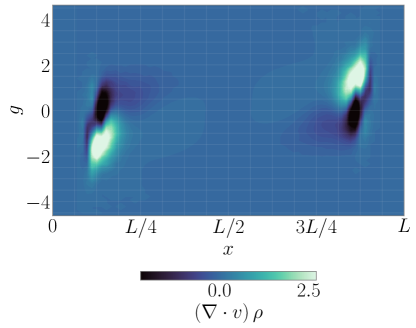
Figure 3: System EPR. Visualization of $\nabla\cdot v(r)$ across the phase space for (1) with $N=2$ and $d=1$ in the variables $x_{t}=x_{t}^{2}-x_{t}^{1}$ and $g_{t}=g_{t}^{2}-g_{t}^{1}$. The system EPR along a trajectory $R_{t}(r)$ of the probability flow (7) can be written as $\dot{s}_{\text{sys}}(t)=\nabla\cdot v(R_{t}(r))$, so that $\nabla\cdot v(r)$ gives insight into how entropy is generated locally by the system. Even though $\mathbb{E}_{\rho}[\nabla\cdot v]=0$ at stationarity, $\nabla\cdot v\neq 0$ pointwise when the system is out of equilibrium. Here, system entropy is locally produced when the two particles collide, and released when they separate.

Given a solution $\rho$ to (3), the Gibbs entropy of the system is defined as

$$S_{\text{sys}}=-\int_{\Omega}\log\rho(r)\rho(r)dr.$$ (12)

At stationarity, $S_{\text{sys}}$ is time-independent, and hence must be preserved by the dynamics. To see how this occurs at the level of the individual degrees of freedom, we can consider the evolution of the stochastic entropy of the system [11, 7] along trajectories of the probability flow ODE 7

$$s_{\text{sys}}(t)=-\log\rho(R_{t}(r)).$$ (13)

From Eq. 8, $S_{\text{sys}}$ may be obtained as an expectation of $s_{\text{sys}}(t)$ at any time $t$ over the initial condition $r$ drawn from $\rho$. We emphasize that our definition of $s_{\text{sys}}(t)$ differs from the one considered in [11, 63], as we study $\log\rho$ along trajectories of the probability flow ODE 7, while these past works studied $\log\rho$ along solutions of the SDE 28. Our definition leads to new expressions for the system and total EPR in terms of $v$. Specifically, we show in (SI appendix) that the system EPR can be written

$$\dot{s}_{\text{sys}}(t) =\nabla\cdot v(R_{t}(r)).$$ (14)

The quantity $\nabla\cdot v$ is visualized over the phase space of our low-dimensional illustrative example in Figure 3, which highlights alternating regions of system entropy production and consumption in the two modes. Equation (14) reveals a stochastic thermodynamic interpretation of nonequilibrium as a state in which the system EPR is nonzero. Moreover, because $S_{\text{sys}}$ is a constant of motion at stationarity, we arrive at the condition

$$\dot{S}_{\text{sys}}=\int_{\Omega}\nabla\cdot v(r)\rho(r)dr=0.$$ (15)

Later, we will make use of (15) as a quantitative test to measure convergence of our learning algorithm. To understand how $\dot{s}_{\text{sys}}$ is distributed spatially in systems with a high-dimensional phase space, we may decompose $\nabla\cdot v$ into a local sum of contributions from individual particles using $v(r)=(v^{1}(r),\ldots,v^{N}(r))$ to obtain

$$\nabla\cdot v(r)=\sum_{i=1}^{N}\nabla_{i}\cdot v^{i}(r),$$ (16)

where $\nabla_{i}$ denotes the gradient with respect to $r^{i}$.

3.2 Total EPR

Assuming that $D$ is invertible, we can alternatively use (3) and (7) to obtain (SI appendix)

$$\dot{s}_{\text{sys}}(t) =\underbrace{|v(R_{t}(r))|_{D^{-1}}^{2}}_{\mathclap{\dot{s}_{\text{tot}}(t)}}-\underbrace{b(R_{t}(r))\cdot D^{-1}v(R_{t}(r))}_{\mathclap{\dot{s}_{\text{m}}(t)}}.$$ (17)

where $|v|^{2}_{D^{-1}}=v^{\mathsf{T}}D^{-1}v$. The first quantity on the right-hand side is non-negative, and can be identified as the total entropy production rate $\dot{s}_{\text{tot}}(t)$ along the flow lines of the probability current $R_{t}(r)$, by analogy with the stochastic identification in [11, 63]. The second term is of indefinite sign even upon averaging over $\rho$, and hence can be identified as the entropy production of the medium $\dot{s}_{\text{m}}(t)$ [64, 65, 22, 19, 11, 4]. Similar to (16), assuming that $D$ is made of $N$ diagonal blocks $D^{i}$, we may decompose

$$|v(r)|_{D^{-1}}^{2}=\sum_{i=1}^{N}|v^{i}(r)|_{D_{i}^{-1}}^{2},$$ (18)

into local contributions from individual particles. Eq. 18 leads to a stochastic thermodynamic interpretation of the condition $v=0$ as a state in which there is no total EPR.

3.3 Global EPR

The global EPR is defined as the Kullback-Leibler divergence between the forward and reverse path measures [19, 4]

$$\dot{S}_{\text{tot}}=\lim_{{T\rightarrow\infty}}\frac{1}{T}\left\langle\log\left(\frac{\mathcal{P}(\phi_{T})}{\mathcal{P}^{\mathsf{R}}(\phi_{T})}\right)\right\rangle,$$ (19)

where $\phi_{T}=\{r_{t}\}_{{0\leq t\leq T}}$ denotes a path through phase space, $\mathcal{P}$ denotes the path measure for (2), $\mathcal{P}^{\mathsf{R}}$ denotes the path measure for a reverse-time dynamics, and the angular brackets denote an average over realizations of the noise in (2). The global EPR can be challenging to compute because it requires a choice of reverse-time dynamics, and the correct one has been a subject of debate [23, 24, 62, 66, 22, 67]. Interestingly, there is a way to construct a reverse-time dynamics such that $\dot{S}_{\text{tot}}$ can be written as an expectation of $\dot{s}_{\text{tot}}$, but it requires again knowledge of $v(r)$. This reverse-time dynamics is the SDE whose solutions have the same statistical properties as the solutions to (2) played in reverse. It reads (SI Appendix)

$$\dot{r}_{t}^{\mathsf{R}}=b(r_{t}^{\mathsf{R}})-2v(r_{t}^{\mathsf{R}})+\sqrt{2D}\,\eta(t),$$ (20)

where $\eta(t)$ is the same Gaussian white noise process as in the forward SDE 2. By a standard path integral argument [68] or an application of the Girsanov theorem [69], when $D$ is invertible we may compute (SI Appendix)

$$\dot{S}_{\text{tot}} =\int_{\Omega}|v(r)|_{D^{-1}}^{2}\rho(r)dr,$$ (21)

which, by Eq. 8, may be understood as the the total EPR $\dot{s}_{\text{tot}}$ averaged over $r$ drawn from $\rho$.

4 Learning Algorithm

4.1 Score

The expressions for $v$, the system EPR, and the total EPR depend on the score $\nabla\log\rho(r)$, which is a high-dimensional function we typically do not have access to. In this section, we develop a machine learning algorithm to approximate it: a graphical summary of the method is given in Figure 1. In addition to providing access to $v$, and therefore to the total and system EPRs, $\nabla\log\rho$ has the important advantage that it is independent of the normalizing constant of $\rho$, which is typically unknown and intractable. This enables us to exploit expressive function classes that need-not represent normalized probability distributions.

4.2 Score Matching

The score $\nabla\log\rho$ can be shown to be the unique minimizer of the loss

$$\mathcal{L}_{\mathsf{sm}}[\hat{h}] =\mathbb{E}_{\rho}\left[\left|\hat{h}\right|^{2}+2\nabla\cdot\hat{h}\right],$$ (22)

$$\nabla\log\rho =\operatorname*{argmin}_{\hat{h}}\mathcal{L}_{\text{sm}}[\hat{h}],$$

where $\mathbb{E}_{\rho}$ denotes expectation over $\rho$. Eq. 22 is known as the “score matching” loss in the machine learning literature [30]. For the reader’s convenience, we provide a derivation of this loss and demonstrate the uniqueness of its minimizers in (SI Appendix).

4.3 Exploiting the Stationary FPE

While a useful loss function, (22) is valid for any data distribution, and does not make use of the fact that $\rho$ solves the stationary FPE (3); it is therefore agnostic to the underlying physics. Intuitively, exploiting our prior knowledge that $\rho$ solves (3) should impose additional structure that can be leveraged to improve the quality of the learned score. As written, (3) is an equation for $\rho$, while we are interested in estimating $\nabla\log\rho$. Dividing by $\rho$ yields a nonlinear equation for the score

$$\nabla\cdot v+v\cdot\nabla\log\rho=0.$$ (23)

Equation 23 may be used to construct a physics-informed loss based on the squared residual [39, 53]

$$\mathcal{L}_{\mathsf{FPE}}[\hat{h}]=\mathbb{E}_{\rho}\left[\left(\nabla\cdot\hat{v}+\hat{v}\cdot\hat{h}\right)^{2}\right],$$ (24)

where $\hat{v}(r)=b(r)-D\hat{h}(r)$. We propose minimization of the composite loss

$$\mathcal{L}[\hat{h}]=\lambda_{1}\mathcal{L}_{\mathsf{sm}}[\hat{h}]+\lambda_{2}\mathcal{L}_{\mathsf{FPE}}[\hat{h}],$$ (25)

which consists of both the physics-agnostic score matching loss $\mathcal{L}_{\mathsf{sm}}$ and the physics-informed loss $\mathcal{L}_{\mathsf{FPE}}$. In our experiments, we find best performance incorporating both terms, and we set $\lambda_{1}=\lambda_{2}=1$ throughout unless otherwise indicated.

4.4 Empirical Loss

In practice, we minimize an empirical approximation of (25)

$$\hat{\mathcal{L}}[\hat{h}] =\frac{\lambda_{1}}{n}\sum_{\alpha=1}^{n}\left(|\hat{h}(r_{\alpha})|^{2}+2\nabla\cdot\hat{h}(r_{\alpha})\right)$$ (26)

$$\qquad+\frac{\lambda_{2}}{n}\sum_{i=1}^{n}\left(\nabla\cdot\hat{v}(r_{\alpha})+\hat{v}(r_{\alpha})\cdot\hat{h}(r_{\alpha})\right)^{2}$$

over a dataset of samples $\{r_{\alpha}\}_{\alpha=1}^{n}$ with each $r_{\alpha}\sim\rho$. We can generate such a dataset by simulating the SDE in (2) with a numerical integration scheme like the Euler-Maruyama method. To make the optimization computationally tractable for high-dimensional systems of particles, we can perform the estimation over an expressive parametric class for $\hat{h}(r)$ such as neural networks, and can use a first-order optimization scheme such as Adam [70] to optimize the parameters. To increase the diversity of the dataset, we can take steps of the SDE 1 between steps of the optimization algorithm, which is similar to online learning and helps prevent overfitting.

4.5 Quantitative Validation

There are several metrics that we can use to verify the accuracy of the learned approximation $\hat{h}$ to $\nabla\log\rho$. The loss in (24) is exactly the squared residual for the stationary score-based FPE (23), and hence provides a quantitative measure of how well the learned score satisfies its governing equation. At optimality, (22) satisfies $\mathcal{L}_{\mathsf{sm}}[\nabla\log\rho]=-\mathbb{E}_{\rho}\left[|\nabla\log\rho|^{2}\right]$ (SI Appendix); deviation from this relation also provides a measure of convergence. Last, we can verify the constraint (15) to ensure that the global EPR is a constant of the motion.

5 Neural Network Architecture

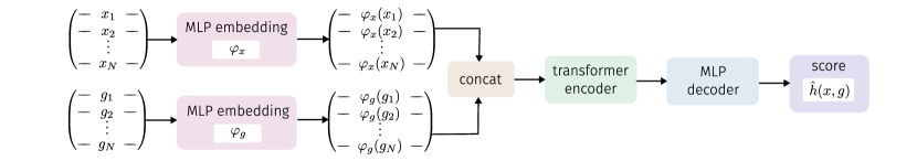
Figure 4: Network Architecture. Depiction of the transformer architecture introduced in this work. The particle positions and orientations are fed into separate multi-layer perceptrons (MLPs) that embed the input into a latent space of higher dimensionality. The embeddings are concatenated particle-wise and fed into a transformer encoder block (SI appendix for further details), where multiple layers of multi-head attention modules learn relevant interactions between particles. The output of the encoder block is decoded by a shared MLP applied to each particle state to obtain the score.

5.1 Permutation symmetry

An important ingredient in our learning algorithm is a proper choice of the neural network used to estimate $\nabla\log\rho$. One guiding principle that can be used for physical problems is to build the symmetries of the system into the network [50]. In addition to its conceptual motivation, this approach has been shown to be statistically advantageous [71]. In (1), the most relevant symmetry group is permutation invariance amongst the particles, which generates complex multi-modal structure in the stationary density $\rho$. Generically, all the configurations generated by permutations will not be present in a given dataset, and this makes it crucial to use a representation of $\nabla\log\rho(r)$ where the permutation invariance is build-in.

5.2 Invariance and equivariance

Permutation invariance at the level of $\rho$ gives rise to permutation equivariance at the level of $\nabla\log\rho$. In a numerical implementation, we can choose to parameterize $\log\rho$ and take its gradient or to parameterize $\nabla\log\rho$ directly. While it seems physically natural to parameterize $\nabla\log\rho$ as a gradient field, state of the art results in diffusion-based generative modeling directly parameterize the score without this added constraint [31, 72, 73], and we follow this approach here. Doing so reduces the number of gradients that must be computed via automatic differentiation during training, and tends to improve performance and stability.

5.3 Specified interactions

A canonical way to construct a permutation equivariant architecture is to consider a pooling operation over the particles – for example, two-point interactions can be captured by a representation of the form $\hat{h}^{i}(r)=\phi\left(\frac{1}{N}\sum_{j=1}^{N}\psi(r^{i},r^{j})\right)$ for a learnable encoder/decoder pair $\psi$ and $\phi$. While such architectures have been successfully applied to interacting particle systems in the past [34], they become expensive to generalize past two-point interactions, and the emergence of effective three-point interactions has already been demonstrated for active matter systems such as motility-induced phase separation [15].

5.4 Transformers

Perhaps the most natural way to proceed is to employ an architecture that can directly learn the relevant order of the interactions in the system. The transformer architecture [74] has emerged as a powerful tool for learning complex interactions in language [75, 76], and is built upon operations (self-attention and token-wise mappings) that are naturally permutation equivariant. In addition to language modeling, transformers currently achieve state of the art in image classification [77, 78], and have been applied to problems such as protein structure prediction [79] and quantum chemistry [80]. Yet, to our knowledge, they have not been used to study interacting particle systems in active matter and stochastic thermodynamics. Transformers also have the advantage that their attention maps can be inspected a-posteriori for insight into the interactions learned by the model [81].

We introduce a transformer architecture that learns interactions between embeddings of the particle positions $x^{i}$ and orientations $g^{i}$ (Figure 4). The output of a series of transformer encoder blocks consisting of self-attention, LayerNorm [82], and particle-wise multi-layer perceptrons (MLPs) is decoded by an additional particle-wise MLP to obtain the score $\hat{h}$. For large numbers of interacting particles (as we will study in the MIPS system), we introduce a modification of this architecture that exploits a spatially-local ansatz to define the score $\hat{h}^{i}$ at the level of the individual particles. Remarkably, in addition to a large gain in memory efficiency, this architecture enables transfer learning to datasets with a larger numbers of particles, where we find physically meaningful predictions without any additional training. We provide an overview of the relevant features of the transformer architecture, including more detail on the constituent elements of the encoder blocks in (SI Appendix).

6 Active swimmers in a trap

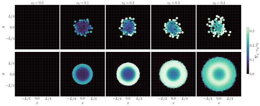
Figure 5: 64 swimmers in a harmonic trap: system EPR. (Top) The contribution of the per-particle orientational degrees of freedom to the system EPR $\nabla_{g^{i}}\cdot v_{g}^{i}$ as a function of the activity $v_{0}$, visualized directly on the particles. For $v_{0}=0$, the system is at equilibrium and the network learns that the system EPR vanishes. As $v_{0}$ increases, nonequilibrium effects emerge, and the particles on the boundary display the highest contribution to the EPR. (Bottom) A spatial map visualizing the typical contribution of a particle at position $(x,y)$ to the system EPR, obtained by averaging the data in the top row over many system snapshots. The map highlights the role of interfacial contributions, and displays a prominent ring at the boundary of the cluster.

6.1 Dynamics

As a first application of our method, we now consider a system of $N=64$ interacting active Ornstein-Uhlenbeck particles in a harmonic trap, similar to what was studied by [15]; this gives rise to a $256$-dimensional many-body FPE in (3). In this case, the system under study is given by (1) with $\epsilon=0.1$, $\gamma=0.1$, $\mu=1$, and where the force $\sum_{j\not=i}f(x^{i}-x^{j})$ has been replaced by the gradient over $x^{i}$ of the potential

$$\Phi(x)=\frac{A}{2}\sum_{i=1}^{N}|x_{i}|^{2}+\frac{1}{2}\sum_{\begin{subarray}{c}i,j=1\\ i\not=j\end{subarray}}^{N}V(x_{i}-x_{j}).$$ (27)

Above, $A=0.05$ and $V(x)=\tfrac{k}{2}\left(2a-|x|\right)^{2}\Theta(2a-|x|)$ with $a=1$ the particle radius, $k=2.5$, and where $\Theta$ denotes the Heaviside step function. To make the system more amenable to learning, we smooth the force slightly to avoid the hard cutoff mediated by $\Theta$ (see SI Appendix for details). Due to the presence of the trap, the system assembles into an active cluster with a dense core and a motile boundary that is similar to the phase separation observed in MIPS. The trap makes the presence of these features more robust to variations in the parameters $\gamma,\epsilon$, and $v_{0}$, which enables us to study the structure of the total and system EPRs as a function of the activity $v_{0}$ at fixed persistence $\gamma$ and bath temperature $\epsilon$. Localizing the cluster also allows us to perform spatial averaging of the EPR, which connects our results with the field-theoretic approach developed in [20]. We stress, however, that our approach does not require this spatial averaging, and we will remove the trap when we study MIPS.

6.2 EPR Decomposition

The contribution of each particle to the system EPR $\nabla_{i}\cdot v^{i}(r)=\nabla_{x^{i}}\cdot v_{x}^{i}(r)+\nabla_{g^{i}}\cdot v_{g}^{i}(r)$ can be decomposed additively into local contributions from the orientational degrees of freedom $g^{i}$ and the translational degrees of freedom $x^{i}$ to understand how they independently contribute to the system EPR. Similarly, the contribution to the total EPR decomposes as $|v^{i}(r)|^{2}=|v_{g}^{i}(r)|^{2}+|v_{x}^{i}(r)|^{2}$. In the following, we make use of these decompositions to isolate further how the total and system EPRs are built up from individual particle contributions.

6.3 Interfacial contributions

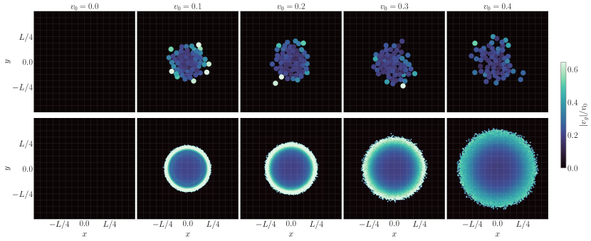
Figure 6: 64 swimmers in a harmonic trap: total EPR. (Top) The contribution of the per-particle orientational degrees of freedom to the total EPR $|v_{g}^{i}|^{2}$ as a function of the activity $v_{0}$, visualized directly on the particles. As in Figure 5, the network learns that the system is at equilibrium for $v_{0}=0$, and the total EPR vanishes. As $v_{0}$ increases, the total EPR is dominated by outlier contributions from particles on the edge of the cluster. (Bottom) A spatial map visualizing the typical contribution of a particle at position $(x,y)$ to the total EPR, obtained by averaging the data in the top row over many system snapshots. The map distills the signal present in the outliers in the top row, and displays a concentrated ring of entropy production at the interface.

We first focus on the contribution of the orientational degrees of freedom to the total EPR $|v_{g}|$ and the system EPR $\nabla_{g}\cdot v_{g}$ (Figures 5 & 6, top). For $v_{0}=0$, the system is at equilibrium and hence the EPR vanishes. As $v_{0}$ is increased, the system becomes increasingly nonequilibrium, and spatial structure begins to emerge in the EPR. Consistent with theoretical predictions [20], we find that both quantities concentrate on the boundary of the cluster. The contribution to the EPR of the system $\nabla_{g}\cdot v_{g}$ increases smoothly with radial distance from the center of the cluster. The contribution to the total entropy production $|v_{g}|$ is similar, but is more dominated by a few outliers on the boundary.

In Figures 16–17 (SI Appendix), we visualize the translational contributions $|v_{x}|$ and $\nabla_{x}\cdot v_{x}$, as well as the EPR $|v|$ and the system EPR $\nabla\cdot v$. $|v_{x}|$ displays similar features to $|v_{g}|$ with slightly lower contrast between the core and the boundary, so that $|v|$ also displays concentration on the interface. We find that $\nabla_{x}\cdot v_{x}\approx-\nabla_{g}\cdot v_{g}$, which causes $\nabla\cdot v$ to roughly vanish pointwise per-particle. Small-scale fluctuations in the particles are present around zero, which together average so that $\mathbb{E}_{\rho}[\nabla\cdot v]\approx 0$ as required by stationarity. We find high accuracy as measured by the residual of the score-based FPE in (23) and the stationarity condition (15) (Figure 18 SI Appendix).

6.4 A spatial map of entropy production

The presence of the trap constrains the shape and location of the cluster, which facilitates averaging in space and in time. To build up a spatial map of the entropy production, we discretize space into a $256\times 256$ grid. We can then sum the particle-wise contributions $\nabla_{g^{i}}\cdot v_{g}^{i}$ and $|v_{g}^{i}|^{2}$ in each grid cell over a dataset of samples, normalizing by the number of particles that appear in each cell in the dataset. The result is a spatial map that describes the typical value of the EPR a particle would attain at a given spatial position. We visualize these spatial maps in Figures 5 & 6 (bottom), where we find a distinct ring of entropy production at the boundary of the core.

6.5 Attention map

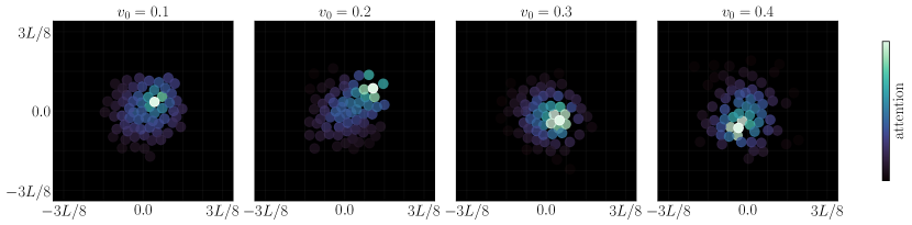
Figure 7: 64 swimmers in a harmonic trap: attention map. The attention map, which quantifies the relevance of other particles for the score of a given particle, for several example swimmers (circled in white) as a function of $v_{0}$. The network learns a spatially-local attention pattern in each case, indicating that the score for each particle is primarily determined by its local neighborhood. Despite this spatial-locality, the learned attention pattern is longer-range than the physical interaction potential.

An advantage of the transformer architecture is that we can visualize the attention map, which gives us insight into which other particles are used to compute the score (and hence the entropy production) of a given particle. To do so, we employed attention rollout [81], which is a simple method to propagate the flow of attention across all heads from layer to layer (for further details, see SI Appendix). The attention map reveals that the network learns a physically-intuitive spatially-local attention pattern, where each particle is primarily influenced by its nearest neighbors (Figure 7). Interestingly, the interactions are still significantly longer-range than those present in the interaction potential for the system.

7 Motility-induced phase separation

\begin{overpic}[width=433.62pt]{figures/mips/EPR.pdf} \put(7.0,41.0){{A}} \put(38.0,41.0){{B}} \put(69.0,41.0){{C}} \end{overpic}

Figure 8: Motility induced phase separation. (A) Reference depiction of the MIPS cluster. (B/C) Particle-wise contributions to the total EPR $|v_{g}^{i}|^{2}$ and the system EPR $\nabla_{g^{i}}\cdot v_{g}^{i}$. Both quantities concentrate on the boundary of the cluster, with sporadic contributions throughout the dilute phase when particles collide. $|v_{g}^{i}|$ vanishes in the center of the cluster, indicating a nontrivial phase dependence in the velocity field. A movie visualizing the evolution of these quantities along stochastic trajectories can be found at this link.

We now consider a system of $N=4096$ interacting particles undergoing motility-induced phase separation, given by (1) with $v_{0}=0.025$, $\mu=1$, $\gamma=10^{-4}$, $\epsilon=0$, and with periodic boundary conditions. In this case, the corresponding many-body FPE is $16,384$-dimensional, and its solution poses a formidable task. Because we consider the athermal, hypoelliptic setting with $\epsilon=0$, the velocity field defined in (6) only depends on the score in the $g$ variables $\nabla_{g}\log\rho$. To target $\nabla_{g}\log\rho$ directly, we consider only the score matching loss (22) and set $\lambda_{2}=0$ in the combined loss (25); the result decouples into equivalent losses for $\nabla_{x}\log\rho$ and $\nabla_{g}\log\rho$, while the physics-informed loss (24) couples the two scores, so they cannot be learned independently. For further details, including an overview of a variant of the denoising score matching loss function [83] we use to reduce computational expense, see (SI Appendix). We learn $\nabla_{g}\log\rho$ on a single dataset with $N=4096$ particles and with a packing fraction $\phi=0.5$, but make use of an architecture that enables us to transfer learn to higher values of $N$ and other values of $\phi$, as we now describe.

7.1 Network architecture

The large number of particles makes it computationally intractable to use the same transformer architecture we used for $N=64$: the self-attention mechanism has time and memory complexities that scale as $\mathcal{O}\left(N^{2}\right)$, which quickly both become prohibitive for large $N$. Nevertheless, Figure 7 shows that the learned attention map is spatially-local in the $N=64$ case, and we expect the same behavior to hold true for the MIPS system. To exploit spatial locality, we developed a transformer architecture defined at the level of an individual particle, which restricts the attention mechanism to a local neighborhood (SI Appendix). This approach has the additional advantage of increasing the effective size of the dataset, because there are many distinct local neighborhoods in a given snapshot of the system. As the size of the attention window is increased, the architecture used for $N=64$ is recovered. Because we define the transformer at the single particle level, our network can be extended to systems with larger $N$ or with a different packing fraction $\phi$, which we demonstrate in this section.

7.2 EPR

Figure 8A shows the MIPS cluster for reference, while Figures 8B & 8C display the orientational contributions to the total EPR $|v_{g}|$ and the system EPR $\nabla_{g}\cdot v_{g}$, respectively. Both quantities are visualized as individual particle contributions without any averaging in space or in time. Consistent with the results for $N=64$ from the previous section, we find that the dominant source of entropy production is at the interface between the gas and solid phases. There are also pockets of entropy production spread sporadically throughout the gas in regions with particle-particle collisions. A movie of a stochastic trajectory, colored by the total and system EPR values, can be found at this link (we recommend downloading the movie for high-resolution viewing).

7.3 Transfer learning toward larger systems

\begin{overpic}[width=433.62pt]{figures/mips/N_transfer.pdf} \end{overpic}

Figure 9: Motility induced phase separation: transfer learning towards larger systems. Our network architecture is defined at the level of individual particles, and depends only on local neighborhoods. This enables us to extend the learned solution from the $N=4096$ training set to larger values of $N$. We consider values of $N$ up to $8\times$ larger, and find physically-consistent predictions in all cases. Movies visualizing the evolution of the EPR along stochastic trajectories can be found at the following links: $N=8192$, $N=16384$, $N=32768$.

Because our neural network architecture is defined at the particle level, it is agnostic to the number of particles $N$ in the system. This means that we can take a single network trained with $N=4096$ and investigate whether it can make reasonable predictions for higher values of $N$ without any re-training. In Figure 9, we show predictions of the total EPR $|v_{g}|$ and system EPR $\nabla_{g}\cdot v_{g}$ as a function of $N$, ultimately scaling up to $32768$ particles. As the number of particles increases, the cluster becomes more well-defined, and the signal in the EPR seen for $N=4096$ becomes increasingly high-resolution. These results highlight the remarkable fact that the local environment learned with $N=4096$ – where dataset generation is significantly cheaper – can be used to make predictions about systems with larger numbers of interacting particles.

7.4 Probability flow

\begin{overpic}[width=433.62pt]{figures/mips/vg.pdf} \put(11.0,60.0){{A}} \put(55.0,60.0){{B}} \end{overpic}

Figure 10: Motility-induced phase separation: probability flow. Particle values of $v_{g}^{i}$ (A) and $g^{i}$ (B), with directionality visualized as arrows for $N=16384$. $v_{g}^{i}$ vanishes in the interior of the solid, but points outward near the solid side of the interface. There is also a layer of particles pointing both inward and outward directly at the interface, corresponding to particles that are exiting and leaving the cluster. The values of $g^{i}$ appear random, and do not have a clear phase dependence by eye, in contrast with $v_{g}^{i}$.

We can use our ability to scale to larger $N$ to investigate the probability flow near the thermodynamic limit: in Figure 10A, we visualize the directionality of $v_{g}^{i}$, and we compare it to $g^{i}$ in Figure 10B. The result reveals a surprising set of observations: $v_{g}^{i}$ vanishes in the solid phase, typically points outwards at the solid edge of the interface, and typically points inwards at the gaseous edge of the interface. While it follows by force-balance that $|v_{x}^{i}|$ must vanish in the solid, an equivalent for $|v_{g}^{i}|$ is nontrivial. This is highlighted when contrasting the particle-wise values of $|v_{g}^{i}|$ with those of $|g^{i}|$. Unlike the $|v_{g}^{i}|$, The $|g^{i}|$ appear random, and by eye, uncorrelated with their phase. This is consistent with the fact that their dynamics is decoupled from the translational degrees of freedom in (1).

Together, these observations reveal a simple picture for the probability flow. Particles in the solid are frozen with $v_{x}^{i}=v_{g}^{i}=0$. Free particles in the gas have $v_{x}^{i}=v_{0}g^{i}$ and $v_{g}^{i}=0$. At particle-particle collisions, $v_{g}^{i}$ becomes nonzero, and entropy is produced. These events are mostly concentrated at the interface between the gas and the solid, where there are particles both exiting and entering the cluster, but also occur sporadically throughout the gas.

7.5 Packing fraction transfer

\begin{overpic}[width=433.62pt]{figures/mips/phi_transfer_N=8192.pdf} \end{overpic}

Figure 11: Motility induced phase separation: transfer learning to other packing fractions. Similar to Figure 9, we find that the learned solution generalizes to other packing fractions $\phi$. Here, we vary $\phi$ at resolution $N=8192$ by varying the size $L$ of the box; for presentation, we rescale the results to the same square. The solution identifies contributions to the EPR from particle-particle collisions in the gaseous phase and at the interface of the gaseous and solid phases. For low and high packing fraction, the EPR diminishes, as the system becomes dominated by a gas or a solid.

In addition to transferring to larger values of $N$, we can investigate the ability of the learned network to transfer to other regimes of the phase diagram, so long as the system parameters defining the particles are fixed. For example, because the score is defined at the level of the local neighborhood of each particle, we expect it to be able to transfer to other packing fractions $\phi$. In Figure 11, we show that a single network trained on a dataset of $N=4096$ particles with $\phi=0.5$ can make physically consistent predictions for a range of values from $\phi=0.01$ to $\phi=0.9$ on a dataset with $N=8192$ particles. For very low packing fraction, there are few particle-particle collisions and no cluster, and the EPR is essentially zero everywhere. As the packing fraction increases, particle-particle collisions begin to occur, so that pockets of entropy production become spread throughout the gas. As a cluster forms for intermediate $\phi$, the EPR becomes concentrated at the interface. As $\phi$ increases further, the cluster becomes dominant, again leaving few regions of entropy production. Analogous figures for $N=4096,N=16384,$ and $N=32768$ are shown in Figures 19-21 (SI Appendix).

Conclusion and future directions

In this work, we demonstrated the capability of machine learning algorithms to learn the entropy production rate and the probability flow of complex interacting particle systems, even in high-dimensional scenarios typically plagued by the curse of dimensionality. In addition to uncovering structure in the EPR, we highlighted that a network trained with a given number of particles $N$ and a fixed packing fraction $\phi$ can generalize to other values of $N$ and $\phi$. As a result, our method paves the way to investigating questions about active systems in the thermodynamic limit.

Physically, we focused on active particles without alignment interactions, and a natural extension of this work is to consider more complex models such as the Vicsek model [84]. Numerically, we considered transformer architectures based on standard self attention modules, but could likely scale to larger systems with less local interactions by incorporating recent advances such as FlashAttention [85, 86]. Mathematically, we focused here on developing algorithms that estimate the score $\nabla\log\rho(x,g)$, and used the score to build the probability flow $v(x,g)=b(x,g)-D\nabla\log\rho(x,g)$. In many cases, particularly when the activity parameter $v_{0}$ is small (such as in MIPS), we may expect the velocity field to be easier to learn than the score. Moreover, learning the score requires a model of the dynamics to construct $v$. It would be useful to develop a loss function that targets $v$ directly, which may be easier to learn in some cases, and which would be directly applicable to experimental data where the dynamics is not known.

Appendix A Entropy Production

A.1 Stochastic Entropy

In this section, we reconsider (2) from an Itô stochastic differential equation (SDE) perspective. We begin by writing (2) as a proper SDE

$$dr_{t}=b(r_{t})dt+\sqrt{2D}dW_{t}$$ (28)

where $W_{t}$ is a Wiener process. To derive an evolution equation for the stochastic entropy, we can apply Itô’s Lemma to $\log\rho$ along trajectories $r_{t}$ of (28). To emphasize terms that vanish only at stationary state, we consider the possibility of a time-dependent $\rho_{t}$:

$$-d\log\rho_{t}(r_{t}) =\partial_{t}\log\rho_{t}(r_{t})dt-\nabla\log\rho_{t}(r_{t})\cdot dr_{t}-\nabla\cdot\left(D\nabla\log\rho_{t}(r_{t})\right)dt$$ (29)

$$=-\partial_{t}\log\rho_{t}(r_{t})dt-\nabla\log\rho(r_{t})\cdot b(r_{t})dt$$

$$\qquad-\nabla\cdot\left(D\nabla\log\rho_{t}(r_{t})\right)dt-\sqrt{2D}\nabla\log\rho_{t}(r_{t})\cdot dW_{t}.$$

We now derive two decompositions for the EPR from (29), similar to the main text.

A.1.1 System EPR

First, we use that $v_{t}=b-D\nabla\log\rho_{t}$ to write that

$$-d\log\rho_{t}(r_{t}) =-\partial_{t}\log\rho_{t}(r_{t})dt-\nabla\log\rho_{t}(r_{t})\cdot b(r_{t})dt+\nabla\cdot v_{t}(r_{t})dt$$ (30)

$$\qquad-\nabla\cdot b(r_{t})dt-\sqrt{2D}\nabla\log\rho_{t}(r_{t})\cdot dW_{t}.$$

Taking an expectation under $\rho_{t}$ and the noise $dW_{t}$ of (30),

$$\mathbb{E}_{\rho_{t},W_{t}}\left[-d\log\rho_{t}(r_{t})\right] =\mathbb{E}_{\rho_{t}}\left[\nabla\cdot v_{t}(r_{t})\right]dt.$$ (31)

In (31), we have used that

$$\mathbb{E}_{\rho_{t}}\left[\partial_{t}\log\rho_{t}\right] =\int_{\Omega}\rho_{t}(r)\frac{\partial_{t}\rho_{t}(r)}{\rho_{t}(r)}dr=\int_{\Omega}\partial_{t}\rho_{t}(r)dr=\frac{d}{dt}\int_{\Omega}\rho_{t}(r)dr=0,$$ (32)

$$\mathbb{E}_{\rho_{t}}[\nabla\cdot b] =\mathbb{E}_{\rho_{t}}[-\nabla\log\rho_{t}\cdot b]$$

where the second relation follows by Stein’s identity (integration by parts).

A.1.2 Total EPR

We now note that

$$-\nabla\log\rho_{t}(r_{t})\cdot b(r_{t}) =-\nabla\log\rho_{t}(r_{t})\cdot\left(v_{t}(r_{t})+D\nabla\log\rho_{t}(r_{t})\right)$$ (33)

$$=-\nabla\log\rho_{t}(r_{t})\cdot v_{t}(r_{t})-|\nabla\log\rho_{t}(r_{t})|_{D}^{2}$$

$$=-\left(D^{-1}(b(r_{t})-v_{t}(r_{t}))\right)\cdot v_{t}(r_{t})-|\nabla\log\rho_{t}(r_{t})|_{D}^{2}$$

$$=|v_{t}(r_{t})|_{D^{-1}}^{2}-b(r_{t})\cdot D^{-1}v_{t}(r_{t})-|\nabla\log\rho_{t}(r_{t})|_{D}^{2}$$

Hence, (29) becomes

$$-d\log\rho_{t}(r_{t}) =-\partial_{t}\log\rho_{t}(r_{t})dt+|v_{t}(r_{t})|_{D^{-1}}^{2}dt-b(r_{t})\cdot D^{-1}v_{t}(r_{t})dt$$

$$\qquad-|\nabla\log\rho_{t}(r_{t})|_{D}^{2}dt-\nabla\cdot\left(D\nabla\log\rho_{t}(r_{t})\right)dt-\sqrt{2D}\nabla\log\rho_{t}(r_{t})\cdot dW_{t}.$$ (34)

We now observe that, by Stein’s identity,

$$\mathbb{E}_{\rho_{t}}\left[-|\nabla\log\rho_{t}(r_{t})|_{D}^{2}\right]=\mathbb{E}_{\rho_{t}}\left[\nabla\cdot\left(D\nabla\log\rho_{t}\right)\right],$$ (35)

so that

$$\mathbb{E}_{\rho_{t},W_{t}}\left[-d\log\rho_{t}(r_{t})\right]=\mathbb{E}_{\rho_{t}}\left[|v_{t}(r_{t})|_{D^{-1}}^{2}\right]dt-\mathbb{E}_{\rho_{t}}\left[b(r_{t})\cdot D^{-1}v_{t}(r_{t})\right]dt.$$ (36)

A.2 Probability Flow Entropy

We now consider two analogous derivations, but along trajectories of the probability flow $p(t)$.

A.2.1 System EPR

To derive the System EPR, we simply apply the chain rule

$$-\frac{d}{dt}\log\rho(R_{t}(r))=-\nabla\log\rho(R_{t}(r))\cdot v(R_{t}(r))$$ (37)

where we have used that $\dot{R}_{t}(r)=v(R_{t}(r))$ by the probability flow ODE 7. Now, by the score-based stationary FPE 23, we have that $\nabla\log\rho(R_{t}(r))\cdot v(R_{t}(r))=-\nabla\cdot v(R_{t}(r))$, so that

$$-\frac{d}{dt}\log\rho(R_{t}(r))=\nabla\cdot v(R_{t}(r)).$$ (38)

A.2.2 Total EPR

To derive the total EPR, we instead use the relation $v=b-D\nabla\log\rho$ to write $\nabla\log\rho=D^{-1}(b-v)$ in (37)

$$-\frac{d}{dt}\log\rho(R_{t}(r)) =-\left(b(R_{t}(r))-v(R_{t}(r))\right)\cdot D^{-1}\cdot v(R_{t}(r))$$

$$=v(R_{t}(r))\cdot D^{-1}v(R_{t}(r))-b(R_{t}(r))\cdot D^{-1}v(R_{t}(r)).$$ (39)

A.3 Importance of $\nabla\cdot v=0$

Here, we elaborate on the relevance of the generalized equilibrium condition $\nabla\cdot v=0$ that we introduced in the main text, and compare it with the more standard definition $v=0$.

A.3.1 Underdamped Langevin Dynamics

We first consider an underdamped Langevin dynamics

$$dx_{t} =u_{t}dt$$ (40)

$$du_{t} =-\gamma u_{t}dt-\nabla_{x}\Phi(x_{t})dt+\sqrt{2\gamma\beta^{-1}}dW_{t}$$

for position $x$, velocity $u$, damping parameter $\gamma>0$, inverse temperature $\beta>0$, and potential $\Phi>0$. The stationary density for (40) is given by

$$\rho(x,u)=Z^{-1}\exp\left(-\beta\Phi(x)-\tfrac{1}{2}\beta|u|^{2}\right),\qquad Z=\int_{\mathbb{R}^{d}\times\mathbb{R}^{d}}\exp\left(-\beta\Phi(x)-\tfrac{1}{2}\beta|u|^{2}\right)dxdu,$$ (41)

so that the score is given by

$$\nabla_{x}\log\rho(x,u) =-\beta\nabla_{x}\Phi(x)$$ (42)

$$\nabla_{u}\log\rho(x,u) =-\beta u.$$

The velocity field for the probability flow is then given by

$$v_{x}(x,u) =u$$ (43)

$$v_{u}(x,u) =-\nabla_{x}\Phi(x).$$

Equation 43 is nonzero in general, unless $x$ is at an extremum of $\Phi$ and $u=0$. Nevertheless,

$$\nabla\cdot v(x,u)=\nabla_{x}\cdot u-\nabla_{u}\cdot\nabla_{x}\Phi(x)=0,$$ (44)

so that the probability flow is incompressible.

A.3.2 Elliptic System

We now consider a more general dynamics than (40) that allows for noise in all coordinates. Let $D=D^{T}$ denote a symmetric positive definite tensor, and let $A=-A^{T}$ denote an antisymmetric tensor. We consider the dynamics

$$dr_{t}=-(D+A)\nabla\Phi(r_{t})dt+\sqrt{2D}dW_{t}.$$ (45)

This system has stationary density given by

$$\rho(r)=Z^{-1}\exp\left(-\Phi(r)\right),\qquad Z=\int_{\Omega}\exp\left(-\Phi(r)\right)dr,$$ (46)

so that the score is given by

$$\nabla\log\rho(r)=-\nabla\Phi(r)$$ (47)

and hence the velocity field $v$ is

$$v(r)=-A\nabla\Phi(r).$$ (48)

The divergence is then given by

$$\nabla\cdot v(r)=-A:\nabla\nabla\Phi(r)=0$$ (49)

because $A$ is antisymmetric and $\nabla\nabla\Phi$ is symmetric, though $v(r)\neq 0$ in general.

Appendix B Time-Reversal

Here, we describe in greater detail the reversal of probability current considered in the main text. Our starting point is the FPE 3. To reverse the probability current, we may re-write this FPE as an equivalent equation with anti-diffusion

$$\partial_{t}\rho_{t}+\nabla\cdot\left(\left(b-2D\nabla\log\rho_{t}\right)\rho_{t}\right)+\nabla\cdot\left(D\nabla\rho_{t}\right)=0.$$ (50)

So that (50) remains well-posed, it must be solved backwards in time from $T$ down to $0$. Equation (50) admits a corresponding reverse-time SDE

$$d\tilde{r}_{t}^{\mathsf{R}}=b(\tilde{r}_{t}^{\mathsf{R}})dt-2D\nabla\log\rho_{t}(\tilde{r}_{t}^{\mathsf{R}})dt+\sqrt{2D}dW_{t}^{\mathsf{R}}$$ (51)

solved backwards from $T$ down to $0$, where $dW_{t}^{\mathsf{R}}$ is a reverse Wiener process. We may then define $r_{t}=\tilde{r}_{T-t}$ to find

$$dr_{t}^{\mathsf{R}}=-b(r_{t}^{\mathsf{R}})dt+2D\nabla\log\rho_{t}(r_{t}^{\mathsf{R}})dt+\sqrt{2D}dW_{t},$$ (52)

where $W_{t}$ is a standard Wiener process. At stationarity, $\rho_{t}(r)=\rho(r)$ and $-b(r)+2D\nabla\log\rho_{t}(r)=b(r)-2v(r)$, so that (52) is (20) written as an Itô SDE.

Appendix C Path KL

C.1 Measure-Theoretic (Girsanov) Derivation

We now consider the SDEs corresponding to (2) and (20), repeated here for simplicity

$$dr_{t} =b(r_{t})dt+\sqrt{2D}dW_{t},$$ (53)

$$dr_{t}^{\mathsf{R}} =-b(r_{t}^{\mathsf{R}})dt+2D\nabla\log\rho_{t}(r_{t}^{\mathsf{R}})dt+\sqrt{2D}dW_{t}.$$

We first observe that the difference in drifts is given by twice the velocity $v_{t}(r)=j_{t}(r)/\rho_{t}(r)$ of the probability flow

$$b(r)-\left(-b(r)+2D\nabla\log\rho_{t}(r)\right)=2b(r)-2D\nabla\log\rho_{t}(r)=2v_{t}(r).$$ (54)

Given this relation, we assume that Novikov’s condition (see [69]) holds, i.e. that

$$\mathbb{E}\left[\exp\left(\int_{0}^{T}|v_{t}(r_{t})|_{D^{-1}}^{2}dt\right)\right]<\infty,$$ (55)

where $\mathbb{E}$ denotes an expectation over the noise in the forward-time dynamics. Because $D$ is assumed full rank, and assuming (55), it follows that (53) fits the conditions of the Girsanov Theorem III, see [69]. Then, assuming a fixed initial condition $r_{0}=r_{0}^{\mathsf{R}}$ for both dynamics, we obtain the Radon-Nikodym derivative between the measure $\mathcal{P}^{\mathsf{R}}$ of the time-reversed process $\phi_{T}^{\mathsf{R}}=\{r^{\mathsf{R}}_{t}\}_{t\in[0,T]}$ and the measure $\mathcal{P}$ of the forward process $\phi_{T}=\{r_{t}\}_{t\in[0,T]}$

$$\frac{\mathcal{P}^{\mathsf{R}}(\phi_{T}|r_{0})}{\mathcal{P}(\phi_{T}|r_{0})}=\exp\left(-\int_{0}^{T}|v_{t}(r_{t})|_{D^{-1}}^{2}dt+\int_{0}^{t}v(r_{t})\cdot D^{-1}(dr_{t}-b(r_{t})dt)\right).$$ (56)

Assuming symmetry in the initial distribution, i.e., $\rho_{T}=\rho^{\mathsf{R}}_{0}$ and $\rho^{\mathsf{R}}_{T}=\rho_{0}$, we have that $\mathcal{P}(\phi_{T})=\mathcal{P}(\phi_{T}|r_{0})\rho_{0}(r_{0})$ and $\mathcal{P}^{\mathsf{R}}(\phi_{T})=\mathcal{P}^{\mathsf{R}}(\phi_{T}|r_{0})\rho_{T}(r_{0})$, so that

$$\dot{S}_{\text{tot}} =-\lim_{T\rightarrow\infty}\frac{1}{T}\mathbb{E}\left[\log\left(\frac{\mathcal{P}^{\mathsf{R}}(\phi_{T})}{\mathcal{P}(\phi_{T})}\right)\right]$$ (57)

$$=-\lim_{T\rightarrow\infty}\frac{1}{T}\mathbb{E}\left[\log\left(\frac{\mathcal{P}^{\mathsf{R}}(\phi_{T}|r_{0})}{\mathcal{P}(\phi_{T}|r_{0})}\right)\right]-\lim_{T\rightarrow\infty}\frac{1}{T}\mathbb{E}\left[\log\left(\frac{\rho_{T}(r_{0})}{\rho_{0}(r_{0})}\right)\right]$$ (58)

$$=\lim_{T\rightarrow\infty}\left\{\frac{1}{T}\mathbb{E}\left[\int_{0}^{T}|v_{t}(r_{t})|_{D^{-1}}^{2}dt\right]-\frac{\sqrt{2}}{T}\mathbb{E}\left[\int_{0}^{T}v_{t}(r_{t})\cdot D^{-1/2}dW_{t}\right]\right\}$$ (59)

$$=\lim_{T\rightarrow\infty}\frac{1}{T}\mathbb{E}\left[\int_{0}^{T}|v_{t}(r_{t})|_{D^{-1}}^{2}dt\right]$$ (60)

$$=\lim_{T\rightarrow\infty}\frac{1}{T}\int_{0}^{T}\int_{\Omega}|v_{t}(r)|_{D^{-1}}^{2}\rho_{t}(r)drdt$$ (61)

$$=\int_{\Omega}|v(r)|_{D^{-1}}^{2}\rho(r)dr.$$ (62)

where $\mathbb{E}$ denotes expectation over the forward process $\phi_{T}=\{r_{t}\}_{t\in[0,T]}$. Above, we used $dr_{t}-b(r_{t})dt=\sqrt{2D}dW_{t}$ which follows from the SDE 2, the martingale property $\mathbb{E}\left[\int_{0}^{T}v(r(t))\cdot D^{-1/2}dW_{t}\right]=0$, that $\lim_{T\rightarrow\infty}\frac{1}{T}\mathbb{E}\left[\log\left(\frac{\rho_{T}(r_{0})}{\rho_{0}(r_{0})}\right)\right]=0$ vanishes as a boundary term, and ergodicity, so that $\rho_{t}(r)\to\rho(r)$ and $v_{t}(r)\rightarrow v(r)=b(r)-D\nabla\log\rho(r)$ as $t\to\infty$ .

C.2 Path Integral (Physicist Style) Derivation

We now consider an analogous derivation to the previous section, instead making use of a path integral formulation [68]. We first write the path measures

$$\mathcal{P}(\phi_{T}) =\frac{1}{Z}\exp\left(-\int_{0}^{T}\mathcal{L}(r_{t},\dot{r}_{t})dt\right),$$ (63)

$$\mathcal{P}^{\mathsf{R}}(\phi_{T}) =\frac{1}{Z}\exp\left(-\int_{0}^{T}\mathcal{L}^{\mathsf{R}}(r_{t},\dot{r}_{t})dt\right),$$

with $\{r_{t}:t\in[0,T]\}$ viewed as a dummy integration variable. We have defined the forward and reverse Lagrangians

$$\mathcal{L}(r,\dot{r}) =\frac{1}{4}\left(\dot{r}_{t}-b(r_{t})\right)\cdot D^{-1}\left(\dot{r_{t}}-b(r_{t})\right)$$ (64)

$$\mathcal{L}^{\mathsf{R}}(r,\dot{r}) =\frac{1}{4}\left(\dot{r}_{t}-b(r_{t})-2v_{t}(r_{t})\right)\cdot D^{-1}\left(\dot{r}_{t}-b(r_{t})-2v_{t}(r_{t})\right)$$

Equation 63 is formal in the sense that the common normalization factor $Z$ is technically infinite, but it is common to both measures and cancels in the ratio defining the EPR. It then follows that

$$\dot{S}_{\text{tot}} =\lim_{T\rightarrow\infty}\frac{1}{T}\left\langle\log\left(\frac{\mathcal{P}(\phi_{T})}{\mathcal{P}^{\mathsf{R}}(\phi_{T})}\right)\right\rangle$$ (65)

$$=\lim_{T\rightarrow\infty}\frac{1}{T}\left\langle\int_{0}^{T}\left(\mathcal{L}(r_{t},\dot{r}_{t})-\mathcal{L}^{\mathsf{R}}(r_{t},\dot{r}_{t})\right)dt\right\rangle.$$

Manipulating the expression for $\mathcal{L}^{\mathsf{R}}$,

$$\mathcal{L}^{\mathsf{R}}(r) =\frac{1}{4}\left(\dot{r}_{t}-b(r_{t})\right)\cdot D^{-1}\left(\dot{r}_{t}-b(r_{t})\right)+|v(r_{t})|_{D^{-1}}^{2}-\left(\dot{r}_{t}-b(r_{t})\right)\cdot D^{-1}v(r_{t})$$ (66)

$$=\mathcal{L}(r_{t})+|v(r_{t})|_{D^{-1}}^{2}-\left(\dot{r}_{t}-b(r_{t})\right)\cdot D^{-1}v(r_{t})$$

$$=\mathcal{L}(r_{t})+|v(r_{t})|_{D^{-1}}^{2}-\sqrt{2D^{-1}}\eta(t)\cdot v(r_{t}).$$

In the last line, we have used the identity $\dot{r}_{t}=b(r_{t})+\sqrt{2D}\eta(t)$, which holds when taking an expectation over the forward paths. Hence, we find that

$$\dot{S}_{\text{tot}} =\lim_{T\rightarrow\infty}\frac{1}{T}\left\langle\int_{0}^{T}\left(|v(r_{t})|_{D^{-1}}^{2}-\sqrt{2D^{-1}}\eta(t)\cdot v(r_{t})\right)dt\right\rangle$$ (67)

$$=\lim_{T\rightarrow\infty}\frac{1}{T}\left\langle\int_{0}^{T}|v(r_{t})|_{D^{-1}}^{2}dt-\int_{0}^{T}\sqrt{2D^{-1}}\eta(t)\cdot v(r_{t})\right\rangle$$

$$=\lim_{T\rightarrow\infty}\frac{1}{T}\left\langle\int_{0}^{T}|v(r_{t})|_{D^{-1}}^{2}dt\right\rangle$$

$$=\int_{\Omega}|v(r)|_{D^{-1}}^{2}\rho(r)dr.$$

Appendix D Review of Score Matching

In this section, we review the score matching loss (22) introduced by [30] and used heavily in the score-based diffusion literature [72, 31].

D.1 Loss Derivation

We first note that to estimate the score a natural objective is the $\mathcal{L}_{2}$ error

$$\tilde{\mathcal{L}}_{\text{sm}}[\hat{h}]=\mathbb{E}_{\rho}\left[|\hat{h}-\nabla\log\rho|^{2}\right].$$ (68)

Expanding the square,

$$\tilde{\mathcal{L}}_{\text{sm}}[\hat{h}]=\mathbb{E}_{\rho}\left[|\hat{h}|^{2}-2\nabla\log\rho\cdot\hat{h}+|\nabla\log\rho|^{2}\right].$$ (69)

The cross term can be integrated by parts (Stein’s identity)

$$\mathbb{E}_{\rho}\left[\nabla\log\rho\cdot\hat{h}\right] =\int_{\Omega}\nabla\log\rho(r)\cdot\hat{h}(r)\rho(r)dr,$$ (70)

$$=\int_{\Omega}\nabla\rho\cdot\hat{h}(r)dr,$$ (71)

$$=-\int_{\Omega}\nabla\cdot\hat{h}(r)\rho(r)dr,$$ (72)

$$=\mathbb{E}_{\rho}\left[-\nabla\cdot\hat{h}\right].$$ (73)

Plugging this back in to (69), we find

$$\tilde{\mathcal{L}}_{\text{sm}}[\hat{h}]=\mathbb{E}_{\rho}\left[|\hat{h}|^{2}+2\nabla\cdot\hat{h}+|\nabla\log\rho|^{2}\right].$$ (74)

Neglecting the constant term $\mathbb{E}_{\rho}\left[|\nabla\log\rho|^{2}\right]$ gives the score matching loss $\mathcal{L}_{\text{sm}}$ in (22), repeated for completeness:

$$\mathcal{L}_{\text{sm}}[h]=\mathbb{E}_{\rho}\left[|h|^{2}+2\nabla\cdot h\right].$$ (75)

Moreover, because (68) is zero for $h=\nabla\log\rho$ and $\tilde{\mathcal{L}}[h]\geq 0$ for all $h$, we find that

$$\mathcal{L}_{\text{sm}}[\nabla\log\rho]=-\mathbb{E}_{\rho}\left[|\nabla\log\rho|^{2}\right]$$ (76)

which is one of the quantitative tests for convergence introduced in the main text.

D.2 Convexity and Global Minimizer

It is clear that (68) is convex in $\hat{h}$ and that its unique minimizer is $\hat{h}=\nabla\log\rho$. We now show that the same holds for $\mathcal{L}_{\text{sm}}$ in (22). We first observe that the first variation with respect to $\hat{h}$ is given by

$$\frac{\delta}{\delta\hat{h}(r)}\mathcal{L}_{\text{sm}}[\hat{h}]=2\hat{h}(r)\rho(r)-2\cdot\nabla\rho(r).$$ (77)

Setting $\frac{\delta}{\delta\hat{h}(r)}\mathcal{L}_{\text{sm}}[h^{*}]=0$ recovers the condition

$$h^{*}(r)=\nabla\log\rho(r),$$ (78)

after division by $\rho$. Hence, the only extreme points $h^{*}(r)$ satisfy $h^{*}(r)=\nabla\log\rho(r)$. Moreover, the second variation is given by

$$\frac{\delta^{2}}{\delta\hat{h}(r)\delta\hat{h}(r^{\prime})}\mathcal{L}_{\text{sm}}[h]=2\rho(r)\delta(r-r^{\prime})\geq 0$$ (79)

so that $\mathcal{L}_{\text{sm}}$ is convex and $h^{*}(r)=\nabla\log\rho(r)$ is the unique global minimizer.

D.3 Denoising Loss

We now derive an equivalent of the loss $\mathcal{L}_{\text{sm}}$ that avoids computation of the divergence $\nabla\cdot\hat{h}$ by use of the transition probabilities for the SDE (2) that generate the density $\rho$. This loss was introduced by [87], but we provide a description here for completeness. Consider a small timestep $\Delta t$, and note that

$$\rho(r_{t+\Delta t})=\int_{\Omega}\rho(r_{t+\Delta t}|r_{t})\rho(r_{t})dr_{t}$$ (80)

by stationarity of the dynamics. It then follows that

$$\nabla\rho(r_{t+\Delta t})=\int_{\Omega}\nabla\rho(r_{t+\Delta t}|r_{t})\rho(r_{t})dr_{t},$$ (81)

where $\nabla=\nabla_{r_{t+\Delta t}}$. Hence, we may write that

$$\mathbb{E}_{\rho}\left[\nabla\log\rho\cdot\hat{h}\right] =\int_{\Omega}\nabla\log\rho(r_{t+\Delta t})\cdot\hat{h}(r_{t+\Delta t})\rho(r_{t+\Delta t})dr_{t+\Delta t}$$ (82)

$$=\int_{\Omega}\nabla\rho(r_{t+\Delta t})\cdot\hat{h}(r_{t+\Delta t})dr_{t+\Delta t}$$

$$=\int_{\Omega}\left(\int_{\Omega}\nabla\rho(r_{t+\Delta t}|r_{t})\rho(r_{t})dr_{t}\right)\cdot\hat{h}(r_{t+\Delta t})dr_{t+\Delta t}$$

$$=\int_{\Omega}\left(\int_{\Omega}\nabla\log\rho(r_{t+\Delta t}|r_{t})\rho(r_{t+\Delta t}|r_{t})\rho(r_{t})dr_{t}\right)\cdot\hat{h}(r_{t+\Delta t})dr_{t+\Delta t}$$

$$=\int_{\Omega\times\Omega}\nabla\log\rho(r_{t+\Delta t}|r_{t})\cdot\hat{h}(r_{t+\Delta t})\rho(r_{t+\Delta t}|r_{t})\rho(r_{t})dr_{t+\Delta t}dr_{t}$$

$$=\mathbb{E}_{r_{t+\Delta t},r_{t}}\left[\nabla\log\rho(r_{t+\Delta t}|r_{t})\cdot\hat{h}(r_{t+\Delta t})\right]$$

Similarly,

$$\mathbb{E}_{\rho}\left[|\hat{h}|^{2}\right] =\int_{\Omega}|\hat{h}(r_{t+\Delta t})|^{2}\rho(r_{t+\Delta t})dr_{t+\Delta t}$$ (83)

$$=\int_{\Omega\times\Omega}|\hat{h}(r_{t+\Delta t})|^{2}\rho(r_{t+\Delta t}|r_{t})\rho(r_{t})dr_{t+\Delta t}dr_{t}$$

$$=\mathbb{E}_{r_{t+\Delta t},r_{t}}\left[|\hat{h}(r_{t+\Delta t})|^{2}\right].$$

Hence, letting $\sim$ denote equivalent up to a constant with respect to $\hat{h}$, we find that

$$\mathbb{E}_{\rho}\left[|\hat{h}-\nabla\log\rho|^{2}\right] =\mathbb{E}_{\rho}\left[|\hat{h}|^{2}\right]-2\mathbb{E}_{\rho}\left[\nabla\log\rho\cdot\hat{h}\right]$$ (84)

$$\qquad+\mathbb{E}_{r_{t+\Delta t},r_{t}}\left[|\nabla\log\rho(r_{t+\Delta t}|r_{t})|^{2}\right]$$

$$\qquad\qquad+\left(\mathbb{E}_{\rho}\left[|\nabla\log\rho|^{2}\right]-\mathbb{E}_{r_{t+\Delta t},r_{t}}\left[|\nabla\log\rho(r_{t+\Delta t}|r_{t})|^{2}\right]\right)$$

$$\sim\mathbb{E}_{\rho}\left[|\hat{h}|^{2}\right]-2\mathbb{E}_{\rho}\left[\nabla\log\rho\cdot\hat{h}\right]+\mathbb{E}_{r_{t+\Delta t},r_{t}}\left[|\nabla\log\rho(r_{t+\Delta t}|r_{t})|^{2}\right]$$

$$=\mathbb{E}_{r_{t+\Delta t},r_{t}}\left[|\hat{h}(r_{t+\Delta t})|^{2}\right]-2\mathbb{E}_{r_{t+\Delta t},r_{t}}\left[\nabla\log\rho(r_{t+\Delta t}|r_{t})\cdot\hat{h}(r_{t+\Delta t})\right]$$

$$\qquad+\mathbb{E}_{r_{t+\Delta t},r_{t}}\left[|\nabla\log\rho(r_{t+\Delta t}|r_{t})|^{2}\right]$$

$$=\mathbb{E}_{r_{t+\Delta t},r_{t}}\left[|\hat{h}(r_{t+\Delta t})-\nabla\log\rho(r_{t+\Delta t}|r_{t})|^{2}\right].$$

For an Euler-Maruyama discretization of (2), we have the exact relation for the transition probability

$$\rho(r_{t+\Delta t}|r_{t}) =\mathsf{N}\left(r_{t}+\Delta tb(r_{t}),2\Delta tD\right),$$ (85)

$$=\frac{1}{Z}\exp\left(-\tfrac{1}{4\Delta t}\left(r_{t+\Delta t}-r_{t}-\Delta tb(r_{t})\right)\cdot D^{-1}\left(r_{t+\Delta t}-r_{t}-\Delta tb(r_{t})\right)\right)$$

Let us define the noise $\xi$ by the relation

$$\sqrt{2\Delta tD}\xi_{t}=r_{t+\Delta t}-r_{t}-\Delta tb(r_{t}).$$ (86)

Then we can compute the transition score exactly,

$$\nabla\log\rho(r_{t+\Delta t}|r_{t}) =-\frac{1}{2\Delta t}D^{-1}\left(r_{t+\Delta t}-r_{t}-\Delta tb(r_{t})\right)$$ (87)

$$=-\left(2\Delta tD\right)^{-1/2}\xi_{t}.$$

Finally, we obtain the “denoising” loss function

$$\mathcal{L}_{\text{d}}[\hat{h}]=\mathbb{E}_{r_{t+\Delta t},r_{t},\xi_{t}}\left[|\hat{h}(r_{t+\Delta t})+\left(2\Delta tD\right)^{-1/2}\xi_{t}|^{2}\right].$$ (88)

By the preceding derivations, up to discretization errors already present in the dataset, $\mathcal{L}_{\text{d}}$ is equivalent to $\mathcal{L}_{\text{sm}}$.

Appendix E Transformer Architecture

In this section, we provide a more detailed description of the particle transformer architecture (Figure 4) introduced in this work.

E.1 Multi-Head Attention

A critical component of the transformer encoder block used in the particle transformer is the multi-head self-attention module. We make use of the scaled dot-product attention introduced by [74],

$$\operatorname{Attention}(Q,K,V)=\operatorname{softmax}\left(\frac{QK^{\mathsf{T}}}{\sqrt{d_{k}}}\right)V.$$ (89)

Above, $Q\in\mathbb{R}^{n_{q}\times d_{q}}$ denotes the matrix of queries, $K\in\mathbb{R}^{n_{v}\times d_{q}}$ denotes the matrix of keys, and $V\in\mathbb{R}^{n_{v}\times d_{v}}$ denotes the matrix of values. Here, we use a multi-head self attention module with $h$ heads that sets the queries, keys, and values equal

$$\operatorname{MultiHead}(X) =\operatorname{Concat}(\operatorname{head}_{1},\ldots,\operatorname{head}_{h})W^{O},$$ (90)

$$\operatorname{head}_{i} =\operatorname{Attention}(XW_{i}^{Q},XW_{i}^{K},XW_{i}^{V}),$$

so that $n_{q}=n_{v}$ and $d_{q}=d_{v}$. Above, $W_{i}^{Q},W_{i}^{K},W_{i}^{V}\in\mathbb{R}^{d_{q}\times d_{h}}$, where $d_{h}$ denotes the dimension of each head. Typically, $d_{h}=d_{q}/h$ with $d_{q}$ a multiple of $h$, and this is the convention we adopt in this work. In our architecture, the tokens will correspond to particles, so we let $n_{q}=N$ and define $d_{e}=d_{q}$ to be the embedding dimension coming from the MLP embeddings (see Figure 4).

E.2 Encoder Block

The encoder block is given by $L$ layers, each consisting of four data transformations applied in succession:

1. A multi-head self-attention module with a residual connection.

2. A LayerNorm [82] block.

3. A single-layer MLP applied to each particle individually with a residual connection.

4. A LayerNorm block.

Mathematically, we can thus describe each layer by the assignments

$$X \leftarrow X+\operatorname{MultiHead}(X),$$ (91)

$$X \leftarrow\operatorname{LayerNorm}(X),$$

$$X \leftarrow X+\psi(X),$$

$$X \leftarrow\operatorname{LayerNorm}(X),$$

where $\psi$ denotes a (shared) MLP applied to each row of $X$. At the first layer, the input $X$ to the multi-head self-attention module is given by the matrix of particle state embeddings. That is, letting $\varphi(x_{i},g_{i})=\left(\varphi_{x}(x_{i})^{\mathsf{T}},\varphi_{g}(g_{i})^{\mathsf{T}}\right)\in\mathbb{R}^{d_{e}}$,

$$X=\begin{pmatrix}\varphi(x_{1})^{\mathsf{T}}\\ \varphi(x_{2})^{\mathsf{T}}\\ \vdots\\ \varphi(x_{N})^{\mathsf{T}}\end{pmatrix}.$$ (92)

The input to each following layer is given by the output of the preceding layer. Importantly, the $\operatorname{MultiHead}(\cdot)$ operation is equivariant with respect to permutations of the rows of its input, i.e., permutations of the particles. The output of the encoder block is then decoded by an MLP, again applied row-wise to the particle states, to produce the approximate score model $\hat{h}$.

E.3 Rollout Attention

The output of $\operatorname{MultiHead}(\cdot)$ at each layer (the attention map) provides a way to visualize and interpret the prediction of the transformer. Yet, it is well-known that the attention map becomes more difficult to interpret deeper in the encoder block because it describes higher-order interactions between the input tokens. Rollout attention is a simple method that combines the attention map of each layer into a single map that can be visualized [81]. Letting the attention map for layer $i$ be given by $A_{i}$, the formula used to obtain the rollout attention map $A$ visualized in Figure 7 is given by

$$A=\prod_{i=1}^{L}\tfrac{1}{2}\left(I+A_{i}\right),$$ (93)

i.e., we take the successive product of the attention map in each layer, accounting for the residual connection by the addition of the identity matrix $I$. The factor $\tfrac{1}{2}$ ensures that the resulting rollout attention map remains normalized.

Appendix F Numerical Experiments

F.1 Smoothed Potential

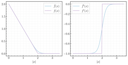
Figure 12: Force smoothing. (Left) Comparison of the smoothed force $\tilde{f}(x)$ given by (95), to the hard cutoff force $f(x)$ given by (94) with $r=1$, as a function of the norm $|x|$. The function values are similar over most of the domain, except for the cutoff point at $|x|=2$. (Right) Comparison of the derivatives $\tilde{f}^{\prime}(x)$ and $f(x)$ as a function of the norm $|x|$. While $f^{\prime}(x)$ is discontinuous, which poses difficulties for learning, $\tilde{f}^{\prime}(x)$ is smooth.

We found that the hard cutoff force listed in the main text

$$f(x)=(2r-|x|)\frac{x}{|x|}\Theta(2r-|x|)$$ (94)

made it difficult to obtain quantitative accuracy with our learning algorithm. This is likely because we use smooth activation functions in our networks, and $f$ has a discontinuous derivative. To alleviate this difficulty, we used a smoothed version of (94)

$$\tilde{f}(x) =\operatorname{softplus}(2r-|x|)\frac{x}{|x|},$$ (95)

$$\operatorname{softplus}(x) =\tfrac{1}{\beta}\log\left(1+\exp(\beta x)\right),$$

with $\beta=7.5$. We found the resulting dynamics to be visually very similar, but the learning algorithm converged faster and to higher accuracy. A comparison of $f(x)$ and $\tilde{f}(x)$ is shown in Figure 12.

F.2 Two Particles on a Ring

\begin{overpic}[width=390.25534pt]{figures/lowd/ring_and_hist.pdf} \put(0.0,25.0){{A}} \put(25.0,25.0){{B}} \end{overpic}

\begin{overpic}[width=325.215pt]{figures/lowd/split_dof_entropy_two_rows.pdf} \put(0.0,75.0){{C}} \put(0.0,40.0){{D}} \end{overpic}

Figure 13: Two active particles on a ring. (A) Diagram of the system. We study a system of two active swimmers in one dimension on the torus. The particles experience a pairwise repulsive force that prevents their overlap. (B) Statistics of the entropy production rate. (C) Decomposition of the probability current into orientational and translational degres of freedom. The orientational degrees of freedom have current dominated at the collision points, while the translational degrees of freedom have current at the collisions and during transitions between the two modes. (D) Decomposition of the system EPR into orientational and translational degrees of freedom. The orientational degrees of freedom have system EPR dominated by the collision point, while the translational degrees of freedom are of larger magnitude and hence similar to $\nabla\cdot v$ in Figure 3 from the main text.

F.2.1 Dynamics

We consider (1) for two particles ($N=2$) in one dimension ($d=1$) with periodic boundary conditions (Figure 13A). In this case, the corresponding four-dimensional dynamics is simple enough to be written explicitly

$$\dot{x}^{1}_{t} =\mu f(x^{1}_{t}-x^{2}_{t})dt+v_{0}g_{t}^{1}+\sqrt{2\epsilon}\,\eta_{x}^{1}(t),$$ (96)

$$\dot{g}^{1}_{t} =-\gamma g^{1}_{t}+\sqrt{2\gamma}\,\eta_{g}^{1}(t),$$

$$\dot{x}^{2}_{t} =\mu f(x^{1}_{t}-x^{2}_{t})+v_{0}g_{t}^{2}+\sqrt{2\epsilon}\,\eta_{x}^{2}(t),$$

$$\dot{g}^{2}_{t} =-\gamma g^{2}_{t}+\sqrt{2\gamma}\,\eta_{g}^{2}(t),$$

where $f(x)$ is given by (95).

F.2.2 Transformed dynamics

In displacement coordinates $x_{t}=x^{1}_{t}-x^{2}_{t}$ and $g_{t}=g^{1}_{t}-g^{2}_{t}$, we can write (96) as

$$\dot{x}_{t} =2\mu f(x_{t})+v_{0}g_{t}+2\sqrt{\epsilon}\,\eta_{x}(t),$$ (97)

$$\dot{g}_{t} =-\gamma g_{t}+2\sqrt{\gamma}\,\eta_{g}(t),$$

where $\eta_{x}(t)=\eta^{1}_{x}(t)-\eta^{2}_{x}(t)$ and $\eta_{g}(t)=\eta^{1}_{g}(t)-\eta^{2}_{g}(t)$ are two new independent white-noises. Equation (97) has the advantage that the phase space is two-dimensional, which enables us to visualize the probability current, probability flow, and the EPR globally as a function of $x$ and $g$, as well as to construct a phase portrait of the probability flow described by (7); these were depicted in Figures 2 & 3.

F.2.3 Numerical implementation and training details

We simulated (97) using the Euler-Maruyama method with a time step of $\Delta t=10^{-3}$, a thermal noise scale $\epsilon=10^{-1}$, and a persistence parameter $\gamma=10^{-1}$ over a horizon $T=100$ to generate a dataset of size $n=10^{6}$. Because there are only two particles, it suffices to use a simpler architecture than the particle transformer, and we adopted a fully connected network with four hidden layers, $256$ neurons per layer, and the GeLU activation function [88]. We used the Adam optimizer with a learning rate of $10^{-6}$, a batch size of $4096$, and trained the network for $200000$ steps. The learning rate was scheduled according to a cosine decay (without warmup), ending at a learning rate of $0$ after $200,000$ steps, according to the function warmup_cosine_decay_schedule in the optax package. Between each epoch, we re-sampled the dataset by taking $250$ steps of the dynamics (97). In (25), we set $\lambda_{1}=\lambda_{2}=1$. We found best performance by learning the scores $s_{x}$ and $s_{g}$ separately, which decouples the learning in (22). The learning of the two scores becomes coupled through the loss term (24).

F.2.4 Quantitative statistics

Figure 13B shows histograms (over independent samples) of the system EPR, along with the contributions from the translational and orientational degrees of freedom. The distribution of $\nabla\cdot v$ is centered around zero (mean $\sim 10^{-3}$), consistent with the requirement that $\mathbb{E}_{\rho}[\nabla\cdot v]=0$ at stationarity. The distribution of $\nabla_{x}\cdot v_{x}$ is centered around a negative value and has a heavy tail, while the distribution of $\nabla_{g}\cdot v_{g}$ is centered around a positive value of opposite sign and nearly equal magnitude. The statistics of the residual for the score-based FPE (23), $v\cdot s$, $|s_{x}|^{2}+\nabla_{x}\cdot s_{x}$ and $|s_{g}|^{2}+\nabla_{g}\cdot s_{g}$ all demonstrate that both scores have been learned to high-accuracy (Figure 15).

F.2.5 Probability current

Figure 13C visualizes a decomposition of the probability current into contributions from the translational and orientational degrees of freedom $|j_{g}|$ and $|j_{x}|$, respectively, as a function of position in phase space $(x,g)$. This decomposition reveals an interesting structure that explains the appearance of limit cycles in the phase portrait (Figure 2D). $|j_{g}|$ is largest near the collisions, which is where $|j_{x}|$ is smallest; these states correspond to a slow-moving particle with a value of $g$ that is changing sign. As the sign flips, the particle begins to move in the other direction. While it does so, $g$ remains roughly constant (as indicated by a small or zero $|j_{g}|$), but $|j_{x}|$ is largest, indicating that the particle is in motion. The system remains in this “free particle” state until another collision occurs on the other side of the ring, where the process repeats. A similar line of reasoning explains the appearance of within-mode limit cycles.

F.2.6 System EPR

Figure 13D visualizes a decomposition of the system EPR into translational and orientational contributions $\nabla_{x}\cdot v_{x}$ and $\nabla_{g}\cdot v_{g}$, as a function of phase space position. We find that $\nabla\cdot v$ is dominated by the contribution from $\nabla_{x}\cdot v_{x}$. $\nabla_{g}\cdot v_{g}$ displays features that are quite similar to $|v_{g}|$, and highlights the interface between the two particles. The regions of highest entropy production in the phase space correspond to when one particle exits the condensed phase. $\nabla_{x}\cdot v_{x}\approx\nabla\cdot v$ shows regions of entropy production and entropy consumption, corresponding to whether the system is entering or leaving a collision. Collectively these regions ensure that $\mathbb{E}\left[\nabla\cdot v\right]\approx 0$. These quantities, as well as the orientational and translational contributions to the total EPR, are also visualized pointwise over phase space in Figure 14, where outliers are more prominent.

\begin{overpic}[width=433.62pt]{figures/lowd/entropy_hist_nospring_density.pdf} \end{overpic}

Figure 14: Two active particles on a ring: pointwise contributions. Pointwise depiction of the total EPR (top) and the system EPR (bottom) over the phase space. Unlike Figure 13, these quantities are not weighted by the density $\rho$. This gives a full picture of both definitions of the EPR, but is more dominated by outlier contributions.

\begin{overpic}[width=325.215pt]{figures/lowd/quantitative_stats_hist.pdf} \end{overpic}

Figure 15: Two active particles on a ring: quantitative convergence statistics. We consider four measures of convergence: the residual for the stationary score-based FPE 23, the condition $\mathbb{E}_{\rho}[v\cdot\nabla\log\rho]=0$, obtained by integrating the condition $\mathbb{E}_{\rho}\left[\nabla\cdot v\right]=0$ by parts, and the condition $\mathbb{E}_{\rho}\left[\nabla\log\rho+\Delta\log\rho\right]=0$, applied separately to the individual components of the score. In all cases, the mean $\mu$ is small in comparison to the standard deviation $\sigma$.

F.3 $N=64$ Particles in a Harmonic Potential

F.3.1 Numerical implementation and training details

We simulated (1) with the potential (27) (subject to the same smoothing as described in (95)) using the Euler-Maruyama method with a time step of $\Delta t=10^{-3}$, a thermal noise scale $\epsilon=10^{-1}$, and a persistence parameter $\gamma=10^{-1}$ over a horizon $T=200$ to generate a dataset of $n=10^{7}$ trajectories. We use the rectified Adam optimizer [89] with a batch size of $64$ and train for $2.5\times 10^{5}$ iterations. We use the transformer architecture described in Figure 4 with four layers in the transformer encoder block, four heads, and two hidden layers in the MLP embedding and decoder. Each MLP (embedding, decoder, and in the transformer encoder block) was selected to have $256$ neurons and the GeLU activation [88]. The embedding dimension $d_{e}=256$ for the transformer encoder block. We employed a cosine warmup and annealing schedule starting and ending at a learning rate of $0$ and peaking at a learning rate of $10^{-4}$ after $10^{4}$ iterations, again according to the function warmup_cosine_decay_schedule in the optax package. Similar to the previous system, we learn $s_{x}$ and $s_{g}$ separately, but couple the learning with $\lambda_{1}=\lambda_{2}=1$.

F.3.2 Boltzmann-informed initialization

For $v_{0}=0$, the system reduces to a Langevin dynamics with stationary measure $\rho_{\mathsf{ss}}(x,g)=\frac{1}{Z}e^{-\Phi(x)/\epsilon}e^{-|g|^{2}/2}$ where $Z$ is the partition function. In this case, the stationary score can be computed exactly, giving the relations

$$\nabla_{x}\log\rho_{\mathsf{ss}}(x,g) =-\frac{1}{\epsilon}\nabla_{x}\Phi(x),$$ (98)

$$\nabla_{g}\log\rho_{\mathsf{ss}}(x,g) =-g.$$

(98) shows that $v=0$ and $\nabla\cdot v=0$ for $v_{0}=0$. We expect that as $v_{0}$ is tuned smoothly away from zero, the score $\nabla\log\rho(x,g)$ can be written as a correction to $\nabla\log\rho_{\mathsf{ss}}(x,g)$. In order to take this into account, we parameterize the score as $s_{x}=-\frac{1}{\epsilon}\nabla_{x}\Phi(x)+N_{x}$ and $s_{g}=-g+N_{g}$ with $N_{x}$ and $N_{g}$ learnable neural networks; this obviates the need to learn $\frac{1}{\epsilon}\nabla_{x}\Phi(x)$ explicitly. Because the neural network weights are initialized randomly around zero, we can view this procedure as shifting the initialization of the network in function space to a ball around the Boltzmann score. Empirically, we find significant improvements in quantitative accuracy metrics when making use of this Boltzmann-informed initialization.

F.3.3 Additional results

Figures 16 & 17 display the quantities $|v_{x}|,\nabla_{x}\cdot v_{x},|v|$ and $\nabla\cdot v$ that were omitted from the main text, while Figure 18 displays the quantitative statistics we used to assess convergence (see captions for discussion).

\begin{overpic}[width=433.62pt]{figures/N64/xdot_combined.pdf} \put(3.0,40.0){{A}} \end{overpic}

\begin{overpic}[width=433.62pt]{figures/N64/v_combined.pdf} \put(3.0,40.0){{B}} \end{overpic}

Figure 16: 64 swimmers in a trap: total EPR (A) [Top] Individual particle contributions from the translational degrees of freedom $|v_{x}^{i}|$ to the total EPR. [Bottom] Spatial map of the translational component of the total EPR $|v_{x}|$, obtained by averaging the data in the top row. Both the particle contributions and the spatial map display a signal concentrated on the interface, but both signals are less clear than the orientational degrees of freedom considered in the main text. (B) [Top] Individual particle contributions to the total EPR $|v^{i}|$. [Bottom] Spatial map, obtained by averaging the data in the top row. Similar to (A), there is a concentrated signal on the interface, but it less clear than the orientational contributions alone.

\begin{overpic}[width=433.62pt]{figures/N64/div_vx_combined.pdf} \put(3.0,40.0){{A}} \end{overpic}

\begin{overpic}[width=433.62pt]{figures/N64/div_v_combined.pdf} \put(3.0,40.0){{B}} \end{overpic}

Figure 17: 64 swimmers in a trap: system EPR (A) [Top] Individual particle contributions from the translational degrees of freedom $\nabla_{x^{i}}\cdot v_{x}^{i}$ to the total EPR. [Bottom] Spatial map of the translational component of the system EPR $\nabla_{x}\cdot v_{x}$, obtained by averaging the data in the top row. The signal is roughly inverted with respect to $\nabla_{g}\cdot v_{g}$, so that $\nabla_{x}\cdot v_{x}\approx-\nabla_{g}\cdot v_{g}$; this is clearest at the level of the spatial map. (B) [Top] Individual particle contributions to the system EPR $\nabla_{i}\cdot v^{i}$. [Bottom] Spatial map, obtained by averaging the data in the top row. Because $\nabla_{x^{i}}\cdot v_{x}^{i}\approx-\nabla_{g^{i}}\cdot v_{g}^{i}$, the particle contributions nearly vanish up to small-scale fluctuations around zero. These fluctuations are an order of magnitude lower than the values of $\nabla_{g^{i}}\cdot v_{g}^{i}$ and $\nabla_{x^{i}}\cdot v_{x}^{i}$ (see colorbar).

\begin{overpic}[width=390.25534pt]{figures/N64/div_v_statistics.pdf} \put(3.0,19.0){{A}} \end{overpic}

\begin{overpic}[width=390.25534pt]{figures/N64/pinn_statistics.pdf} \put(3.0,19.0){{B}} \end{overpic}

\begin{overpic}[width=390.25534pt]{figures/N64/ibp_statistics.pdf} \put(3.0,19.0){{C}} \end{overpic}

\begin{overpic}[width=390.25534pt]{figures/N64/v_times_s_statistics.pdf} \put(3.0,19.0){{D}} \end{overpic}

Figure 18: 64 Particles: quantitative convergence statistics. Because each quantity considered here consists of a sum of $N$ terms, we normalize by the number of particles. (A) Distribution of $\nabla\cdot v=\sum_{i=1}^{N}\nabla_{i}\cdot v^{i}$ over snapshots of the system. By stationarity of the Gibbs entropy, $\partial_{t}\mathbb{E}_{\rho}\left[\log\rho\right]=0$, we require that $\mathbb{E}_{\rho}\left[\nabla\cdot v\right]=0$. For each value of $v_{0}$, we find a small mean value $\mu$ and a small standard deviation $\sigma$. This indicates that $\mathbb{E}_{\rho}[\nabla\cdot v]\approx 0$. Interestingly, the small value of $\sigma$ indicates $\nabla\cdot v\approx 0$ on each snapshot, which is not strictly required for convergence. (B) Distribution of the score-based stationary FPE ((23)) residual, $\nabla\cdot v+v\cdot s$, over system snapshots. To satisfy the stationary FPE, this quantity should be zero pointwise. We find low mean values $\mu$ and low standard deviations $\sigma$ in all cases, indicating that this is approximately satisfied. (C) Distribution of $|\nabla\log\rho|^{2}+\Delta\log\rho$. By integration by parts, we require that $\mathbb{E}_{\rho}\left[|\nabla\log\rho|^{2}+\Delta\log\rho\right]=0$. We find a low mean value in all cases. The standard deviation is orders of magnitude higher, indicating that this quantity does not vanish pointwise (which is not required for convergence). (D) Distribution of $v\cdot\nabla\log\rho$ over snapshots. By integration by parts, $\mathbb{E}_{\rho}\left[\nabla\cdot v\right]=\mathbb{E}_{\rho}\left[-v\cdot\nabla\log\rho\right]=0$, so that this quantity should vanish in expectation by stationarity of the Gibbs entropy. Consistent with (A), we find a low $\mu$ and a low $\sigma$, indicating that it approximately vanishes both in expectation and pointwise.

F.4 Motility-Induced Phase Separation

\begin{overpic}[width=433.62pt]{figures/mips/phi_transfer_N=4096.pdf} \end{overpic}

Figure 19: Motility induced phase separation. Packing fraction generalization. Packing fraction generalization with $N=4096$.

\begin{overpic}[width=433.62pt]{figures/mips/phi_transfer_N=16384.pdf} \end{overpic}

Figure 20: Motility induced phase separation. Packing fraction generalization. Packing fraction generalization with $N=16384$.

\begin{overpic}[width=433.62pt]{figures/mips/phi_transfer_N=32768.pdf} \end{overpic}

Figure 21: Motility induced phase separation. Packing fraction generalization. Packing fraction generalization with $N=32768$.

F.5 Dataset generation

We simulated (1) using the Euler-Maruyama method in the athermal regime with $\epsilon=0$, a persistence parameter $\gamma=10^{-4}$, a timestep of $\Delta t=10^{-1}$, a self-propulsion velocity $v_{0}=0.025$ and a packing fraction of $\phi=0.5$. These parameters were chosen to ensure the system was in the motility-induced phase separation regime. Due to the large number of interacting particles, it is computationally expensive to generate a large dataset of thermalized independent samples, as was done in the previous two examples. Instead, we simulated $12$ independent initial conditions until time $1/\gamma$ and verified that a cluster had formed. Then we generated a trajectory of $10,000$ samples per initial condition separated by a time lag $\tau=0.02/\gamma=20$.

F.6 Network Architecture

We define the score $s^{i}$ for each particle $i$ using the architecture in Figure 4; to reduce time and memory complexity, the input to the encoder block is only the embedding for particle $i$ along with the embeddings for the $N_{\text{neighbors}}$ nearest neighbors. The output of the network is then a matrix of size $(N_{\text{neighbors}}+1)\times d$. These represent the score $s^{i}$ along with a set of rich features for each neighboring particle used to compute $s^{i}$; the latter are discarded, so that as $N_{\text{neighbors}}\rightarrow N$, we recover the architecture used for $N=64$ defined at the level of the full system. To ensure equivariance amongst particles, we share weights in the embedding, encoder, and decoder between all particles.

F.7 Scale separation and singularity

In the athermal limit $\epsilon=0$, we found it more challenging to maintain the zero system EPR condition $\mathbb{E}_{\rho}\left[\nabla\cdot v\right]=0$ than in the thermal regime. To see analytically why this may be the case, note that

$$v_{x}(x,g) =-\nabla_{x}\Phi(x),$$ (99)

$$v_{g}(x,g) =-\gamma g-\gamma\nabla_{g}\log\rho(x,g).$$

for $\epsilon=0$. Hence,

$$\nabla\cdot v=-\Delta_{x}\Phi(x)-\gamma d-\gamma\Delta_{g}\log\rho(x,g),$$ (100)

so that the condition $\mathbb{E}_{\rho}\left[\nabla\cdot v\right]=0$ reads

$$\mathbb{E}_{\rho}\left[-\Delta_{x}\Phi(x)\right]=\gamma d+\gamma\mathbb{E}_{\rho}\left[\Delta_{g}\log\rho(x,g)\right].$$ (101)

The Laplacian term $-\Delta_{x}\Phi(x)$ (for the hard cutoff potential) is given by

$$-\Delta_{x}\Phi(x)=\sum_{i,j=1}^{N}\left(\frac{2r(d-1)}{|x^{i}-x^{j}|}-d\right)\Theta\left(2r-|x^{i}-x^{j}|\right).$$ (102)

In the solid, $|x^{i}-x^{j}|\sim 2r$, so that each term in the sum is $\mathcal{O}(1)$, and the overall Laplacian can be as large as $\mathcal{O}(N)$. For the small $\gamma\sim 10^{-4}$ values needed to induce MIPS, this creates a difficult scale-separation problem for a learning algorithm, as $\Delta_{g}\log\rho(x,g)$ must be of order $\mathcal{O}(1/\gamma)$ to cancel the contribution from $\Delta_{x}\Phi(x)$. Moreover, because the stationary density for $v_{0}=0$ is singular,

$$\rho_{\text{ss}}(x,g)=\frac{1}{Z}\delta\left(\nabla\Phi(x)\right)\exp\left(-\frac{1}{2}|g|^{2}\right),$$ (103)

it is not clear how to initialize to avoid this problem. By contrast, in the thermal setting

$$v_{x}(x,g) =-\nabla_{x}\Phi(x)-\epsilon\nabla_{x}\log\rho(x,g),$$ (104)

$$v_{g}(x,g) =-\gamma g-\gamma\nabla_{g}\log\rho(x,g).$$

Stationarity of the Gibbs entropy $\mathbb{E}_{\rho}\left[\nabla\cdot v\right]=0$ becomes

$$\mathbb{E}_{\rho}\left[-\Delta_{x}\Phi(x)\right]-\epsilon\mathbb{E}_{\rho}\left[\Delta_{x}\log\rho(x,g)\right]=-\gamma d-\gamma\mathbb{E}_{\rho}\left[\Delta_{g}\log\rho(x,g)\right].$$ (105)

Here, the scale-separation problem is offloaded to the score in $x$. This can be seen most clearly by observing that the stationary score is now well-defined for $v_{0}=0$,

$$\nabla_{x}\log\rho_{\text{ss}} =-\frac{1}{\epsilon}\nabla\Phi(x),$$ (106)

$$\nabla_{g}\log\rho_{\text{ss}} =-g.$$

We exploited this observation in the $N=64$ system via the introduction of a Boltzmann-informed initialization. However, to ensure a well-defined MIPS cluster for finite $\epsilon$, we must take $\epsilon$ very small. While the Boltzmann-informed initialization avoids the need to learn a term of order $1/\epsilon$, such a term is still included in the score parameterization, which makes the loss function poorly conditioned.

F.8 Loss function

To sidestep these issues, we make use of the denoising loss function described in Section D.3 to learn only the score in $g$. Importantly, we add noise in the $x$ variables, which corresponds to taking a step along a thermal dynamics (where the $x$ score is nearly singular, but the $g$ score is well-behaved) starting from athermal data. This approach ensures that there is a well-defined boundary of the cluster, avoids the need to learn a term of large magnitude, and is structured so that cancellation of the equilibrium force term $-\nabla_{x}\Phi(x)$ to ensure $\mathbb{E}\left[\nabla\cdot v\right]=0$ will happen in the score in $x$, which we do not learn. We have already seen in the $N=64$ example that $\nabla_{x}\cdot v_{x}\approx-\nabla_{g}\cdot v_{g}$ and that there is a rich signal contained in $v_{g}$ alone, which further justifies restricting to $v_{g}$.

F.9 Training details

We set $N_{\text{neighbors}}=64$ and otherwise use identical network hyperparameters as in the example of $64$ active swimmers. We use a cosine warmup and annealing schedule, peaking at a learning rate of $10^{-6}$ after $10,000$ steps and ending at a learning rate of $0$ after $500,000$ steps. Because all terms in the denoising loss split into contributions from individual particles, and because the network is defined at the particle level, we consider the particles as datapoints and batch over the particles themselves (ensuring that batches never include particles from two separate snapshots of the system). We use a batch size of $1024$ particles. In the denoising loss, we use a noise with standard deviation $\sigma=0.01$ and neglect the drift term $b$ in the denoising loss because it is higher-order in $\Delta t$.

F.10 Additional results

Figures 19-21 show the ability of the learned network (trained with $N=4096$ and packing fraction $\phi=0.5$) to generalize to other values of $\phi$ for $N=4096,N=16384$, and $N=32768$; only $N=8192$ was considered in the main text. In all cases, the predictions are physically reasonable.

References

- Marchetti et al. [2013] M. C. Marchetti, J. F. Joanny, S. Ramaswamy, T. B. Liverpool, J. Prost, Madan Rao, and R. Aditi Simha. Hydrodynamics of soft active matter. Reviews of Modern Physics, 85(3):1143–1189, 2013.
- Fodor et al. [2022] Etienne Fodor, Robert L. Jack, and Michael E. Cates. Irreversibility and Biased Ensembles in Active Matter: Insights from Stochastic Thermodynamics. Annual Review of Condensed Matter Physics, 13(1):215–238, 2022.
- O’Byrne et al. [2022] J. O’Byrne, Y. Kafri, J. Tailleur, and F. van Wijland. Time irreversibility in active matter, from micro to macro. Nature Reviews Physics, 4(3):167–183, 2022.
- Lebowitz and Spohn [1999] Joel L. Lebowitz and Herbert Spohn. A Gallavotti–Cohen-Type Symmetry in the Large Deviation Functional for Stochastic Dynamics. Journal of Statistical Physics, 95(1):333–365, 1999.
- Parrondo et al. [2009] J M R Parrondo, C Van den Broeck, and R Kawai. Entropy production and the arrow of time. New Journal of Physics, 11(7):073008, 2009.
- Jarzynski [2011] Christopher Jarzynski. Equalities and Inequalities: Irreversibility and the Second Law of Thermodynamics at the Nanoscale. Annual Review of Condensed Matter Physics, 2(1):329–351, 2011.
- Seifert [2012] Udo Seifert. Stochastic thermodynamics, fluctuation theorems, and molecular machines. Reports on Progress in Physics, 75(12):126001, 2012.
- Bodineau and Derrida [2007] Thierry Bodineau and Bernard Derrida. Cumulants and large deviations of the current through non-equilibrium steady states. Comptes Rendus Physique, 8(5):540–555, 2007.
- Battle et al. [2016] Christopher Battle, Chase P. Broedersz, Nikta Fakhri, Veikko F. Geyer, Jonathon Howard, Christoph F. Schmidt, and Fred C. MacKintosh. Broken detailed balance at mesoscopic scales in active biological systems. Science, 352(6285):604–607, 2016.
- Bertini et al. [2015] Lorenzo Bertini, Alberto De Sole, Davide Gabrielli, Giovanni Jona-Lasinio, and Claudio Landim. Macroscopic fluctuation theory. Reviews of Modern Physics, 87(2):593–636, 2015.
- Seifert [2005] Udo Seifert. Entropy Production along a Stochastic Trajectory and an Integral Fluctuation Theorem. Physical Review Letters, 95(4):040602, 2005.
- Gomez-Marin et al. [2008] A. Gomez-Marin, J. M. R. Parrondo, and C. Van den Broeck. The “footprints” of irreversibility. Europhysics Letters, 82(5):50002, 2008.
- Pietzonka and Seifert [2018] Patrick Pietzonka and Udo Seifert. Entropy production of active particles and for particles in active baths. Journal of Physics A: Mathematical and Theoretical, 51(1):01LT01, 2018.
- Fodor et al. [2016] Etienne Fodor, Cesare Nardini, Michael E. Cates, Julien Tailleur, Paolo Visco, and Frederic Van Wijland. How Far from Equilibrium Is Active Matter? Physical Review Letters, 117(3):038103, 2016.
- Martin et al. [2021] David Martin, Jeremy O’Byrne, Michael E. Cates, Etienne Fodor, Cesare Nardini, Julien Tailleur, and Frederic Van Wijland. Statistical mechanics of active Ornstein-Uhlenbeck particles. Physical Review E, 103(3):032607, 2021.
- Speck [2018] Thomas Speck. Active Brownian particles driven by constant affinity. Europhysics Letters, 123(2):20007, 2018.
- Shankar and Marchetti [2018] Suraj Shankar and M. Cristina Marchetti. Hidden entropy production and work fluctuations in an ideal active gas. Physical Review E, 98(2):020604, 2018.
- Dadhichi et al. [2018] Lokrshi Prawar Dadhichi, Ananyo Maitra, and Sriram Ramaswamy. Origins and diagnostics of the nonequilibrium character of active systems. Journal of Statistical Mechanics: Theory and Experiment, 2018(12):123201, 2018.
- Crooks [1999] Gavin E. Crooks. Entropy production fluctuation theorem and the nonequilibrium work relation for free energy differences. Physical Review E, 60(3):2721–2726, 1999.
- Nardini et al. [2017] Cesare Nardini, Étienne Fodor, Elsen Tjhung, Frédéric van Wijland, Julien Tailleur, and Michael E. Cates. Entropy Production in Field Theories without Time-Reversal Symmetry: Quantifying the Non-Equilibrium Character of Active Matter. Physical Review X, 7(2):021007, 2017.
- Borthne et al. [2020] Oyvind L. Borthne, Etienne Fodor, and Michael E. Cates. Time-reversal symmetry violations and entropy production in field theories of polar active matter. New Journal of Physics, 22(12):123012, 2020.
- Chetrite and Gawedzki [2008] Raphael Chetrite and Krzysztof Gawedzki. Fluctuation relations for diffusion processes. Communications in Mathematical Physics, 282(2):469–518, 2008.
- Mandal et al. [2017] Dibyendu Mandal, Katherine Klymko, and Michael R. DeWeese. Entropy Production and Fluctuation Theorems for Active Matter. Physical Review Letters, 119(25):258001, 2017.
- Caprini et al. [2018] Lorenzo Caprini, Umberto Marini Bettolo Marconi, Andrea Puglisi, and Angelo Vulpiani. Comment on “Entropy Production and Fluctuation Theorems for Active Matter”. Physical Review Letters, 121(13):139801, 2018.
- Martiniani et al. [2019] Stefano Martiniani, Paul M. Chaikin, and Dov Levine. Quantifying Hidden Order out of Equilibrium. Physical Review X, 9(1):011031, 2019.
- Ro et al. [2022] Sunghan Ro, Buming Guo, Aaron Shih, Trung V. Phan, Robert H. Austin, Dov Levine, Paul M. Chaikin, and Stefano Martiniani. Model-Free Measurement of Local Entropy Production and Extractable Work in Active Matter. Physical Review Letters, 129(22):220601, 2022.
- Li et al. [2019] Junang Li, Jordan M. Horowitz, Todd R. Gingrich, and Nikta Fakhri. Quantifying dissipation using fluctuating currents. Nature Communications, 10(1):1666, 2019.
- Otsubo et al. [2020] Shun Otsubo, Sosuke Ito, Andreas Dechant, and Takahiro Sagawa. Estimating entropy production by machine learning of short-time fluctuating currents. Physical Review E, 101(6), 2020.
- Otsubo et al. [2022] Shun Otsubo, Sreekanth K. Manikandan, Takahiro Sagawa, and Supriya Krishnamurthy. Estimating time-dependent entropy production from non-equilibrium trajectories. Communications Physics, 5(1):1–10, 2022.
- Hyvarinen [2005] Aapo Hyvarinen. Estimation of Non-Normalized Statistical Models by Score Matching. Journal of Machine Learning Research, 6(24):695–709, 2005.
- Song et al. [2021a] Yang Song, Jascha Sohl-Dickstein, Diederik P. Kingma, Abhishek Kumar, Stefano Ermon, and Ben Poole. Score-Based Generative Modeling through Stochastic Differential Equations. arXiv:2011.13456, 2021a.
- Albergo and Vanden-Eijnden [2023] Michael S. Albergo and Eric Vanden-Eijnden. Building Normalizing Flows with Stochastic Interpolants. arXiv:2209.15571, 2023.
- Albergo et al. [2023] Michael S. Albergo, Nicholas M. Boffi, and Eric Vanden-Eijnden. Stochastic Interpolants: A Unifying Framework for Flows and Diffusions. arXiv:2303.08797, 2023.
- Boffi and Vanden-Eijnden [2023] Nicholas M. Boffi and Eric Vanden-Eijnden. Probability flow solution of the Fokker–Planck equation. Machine Learning: Science and Technology, 4(3):035012, 2023.
- Cates and Tailleur [2015] Michael E. Cates and Julien Tailleur. Motility-Induced Phase Separation. Annual Review of Condensed Matter Physics, 6(1):219–244, 2015.
- Noe et al. [2019] Frank Noe, Simon Olsson, Jonas Kohler, and Hao Wu. Boltzmann generators: Sampling equilibrium states of many-body systems with deep learning. Science, 365(6457), 2019.
- Khoo et al. [2018] Yuehaw Khoo, Jianfeng Lu, and Lexing Ying. Solving for high dimensional committor functions using artificial neural networks. arXiv:1802.10275, 2018.
- Khoo et al. [2020] Yuehaw Khoo, Jianfeng Lu, and Lexing Ying. Solving parametric PDE problems with artificial neural networks. European Journal of Applied Mathematics, pages 1–15, 2020.
- Raissi et al. [2019] M. Raissi, P. Perdikaris, and G. E. Karniadakis. Physics-informed neural networks: A deep learning framework for solving forward and inverse problems involving nonlinear partial differential equations. Journal of Computational Physics, 378:686–707, 2019.
- Bar-Sinai et al. [2019] Yohai Bar-Sinai, Stephan Hoyer, Jason Hickey, and Michael P. Brenner. Learning data-driven discretizations for partial differential equations. Proceedings of the National Academy of Sciences, 116(31):15344–15349, 2019.
- Gabrie et al. [2022] Marylou Gabrie, Grant M. Rotskoff, and Eric Vanden-Eijnden. Adaptive Monte Carlo augmented with normalizing flows. Proceedings of the National Academy of Sciences, 119(10):e2109420119, 2022.
- Brunton et al. [2016] Steven L. Brunton, Joshua L. Proctor, and J. Nathan Kutz. Discovering governing equations from data by sparse identification of nonlinear dynamical systems. Proceedings of the National Academy of Sciences, 113(15):3932–3937, 2016.
- Lusch et al. [2018] Bethany Lusch, J. Nathan Kutz, and Steven L. Brunton. Deep learning for universal linear embeddings of nonlinear dynamics. Nature Communications, 9(1):4950, 2018.
- Rudy et al. [2017] Samuel H. Rudy, Steven L. Brunton, Joshua L. Proctor, and J. Nathan Kutz. Data-driven discovery of partial differential equations. Science Advances, 3(4), 2017.
- Nusken and Richter [2021] Nikolas Nusken and Lorenz Richter. Solving high-dimensional Hamilton–Jacobi–Bellman PDEs using neural networks: perspectives from the theory of controlled diffusions and measures on path space. Partial Differential Equations and Applications, 2(4):48, 2021.
- E et al. [2021] Weinan E, Jiequn Han, and Arnulf Jentzen. Algorithms for solving high dimensional PDEs: from nonlinear Monte Carlo to machine learning. Nonlinearity, 35(1):278, 2021.
- E and Yu [2018] Weinan E and Bing Yu. The Deep Ritz Method: A Deep Learning-Based Numerical Algorithm for Solving Variational Problems. Communications in Mathematics and Statistics, 6(1):1–12, 2018.
- Kovachki et al. [2023] Nikola Kovachki, Zongyi Li, Burigede Liu, Kamyar Azizzadenesheli, Kaushik Bhattacharya, Andrew Stuart, and Anima Anandkumar. Neural Operator: Learning Maps Between Function Spaces With Applications to PDEs. Journal of Machine Learning Research, 24(89):1–97, 2023.
- Li et al. [2020] Zongyi Li, Nikola Kovachki, Kamyar Azizzadenesheli, Burigede Liu, Kaushik Bhattacharya, Andrew Stuart, and Anima Anandkumar. Fourier Neural Operator for Parametric Partial Differential Equations. arXiv:2010.08895, 2020.
- Carleo et al. [2019] Giuseppe Carleo, Ignacio Cirac, Kyle Cranmer, Laurent Daudet, Maria Schuld, Naftali Tishby, Leslie Vogt-Maranto, and Lenka Zdeborová. Machine learning and the physical sciences. Reviews of Modern Physics, 91(4):045002, 2019.
- Brunton et al. [2020] Steven L. Brunton, Bernd R. Noack, and Petros Koumoutsakos. Machine Learning for Fluid Mechanics. Annual Review of Fluid Mechanics, 52(1):477–508, 2020.
- Supekar et al. [2023] Rohit Supekar, Boya Song, Alasdair Hastewell, Gary P. T. Choi, Alexander Mietke, and Jorn Dunkel. Learning hydrodynamic equations for active matter from particle simulations and experiments. Proceedings of the National Academy of Sciences, 120(7):e2206994120, 2023.
- Karniadakis et al. [2021] George Em Karniadakis, Ioannis G. Kevrekidis, Lu Lu, Paris Perdikaris, Sifan Wang, and Liu Yang. Physics-informed machine learning. Nature Reviews Physics, 3(6):422–440, 2021.
- Kochkov et al. [2021] Dmitrii Kochkov, Jamie A. Smith, Ayya Alieva, Qing Wang, Michael P. Brenner, and Stephan Hoyer. Machine learning–accelerated computational fluid dynamics. Proceedings of the National Academy of Sciences, 118(21):e2101784118, 2021.
- Carleo and Troyer [2017] Giuseppe Carleo and Matthias Troyer. Solving the quantum many-body problem with artificial neural networks. Science, 355(6325):602–606, 2017.
- Hermann et al. [2020] Jan Hermann, Zeno Schatzle, and Frank Noe. Deep-neural-network solution of the electronic Schrodinger equation. Nature Chemistry, 12(10):891–897, 2020.
- Qiao et al. [2020] Zhuoran Qiao, Matthew Welborn, Animashree Anandkumar, Frederick R. Manby, and Thomas F. Miller III. OrbNet: Deep Learning for Quantum Chemistry Using Symmetry-Adapted Atomic-Orbital Features. The Journal of Chemical Physics, 153(12):124111, 2020.
- Pfau et al. [2020] David Pfau, James S. Spencer, Alexander G. de G. Matthews, and W. M. C. Foulkes. Ab-Initio Solution of the Many-Electron Schrödinger Equation with Deep Neural Networks. Physical Review Research, 2(3):033429, 2020.
- Paoluzzi et al. [2016] M. Paoluzzi, C. Maggi, U. Marini Bettolo Marconi, and N. Gnan. Critical phenomena in active matter. Physical Review E, 94(5):052602, 2016.
- Szamel [2014] Grzegorz Szamel. Self-propelled particle in an external potential: Existence of an effective temperature. Physical Review E, 90(1):012111, 2014.
- Flenner et al. [2016] Elijah Flenner, Grzegorz Szamel, and Ludovic Berthier. The nonequilibrium glassy dynamics of self-propelled particles. Soft Matter, 12(34):7136–7149, 2016.
- Caprini et al. [2019] Lorenzo Caprini, Umberto Marini Bettolo Marconi, Andrea Puglisi, and Angelo Vulpiani. The entropy production of Ornstein–Uhlenbeck active particles: a path integral method for correlations. Journal of Statistical Mechanics: Theory and Experiment, 2019(5):053203, 2019.
- Pigolotti et al. [2017] Simone Pigolotti, Izaak Neri, Edgar Roldan, and Frank Julicher. Generic Properties of Stochastic Entropy Production. Physical Review Letters, 119(14):140604, 2017.
- Marconi et al. [2017] Umberto Marini Bettolo Marconi, Andrea Puglisi, and Claudio Maggi. Heat, temperature and Clausius inequality in a model for active Brownian particles. Scientific Reports, 7(1):46496, 2017.
- Puglisi and Marini Bettolo Marconi [2017] Andrea Puglisi and Umberto Marini Bettolo Marconi. Clausius Relation for Active Particles: What Can We Learn from Fluctuations. Entropy, 19(7):356, 2017.
- Dabelow et al. [2019] Lennart Dabelow, Stefano Bo, and Ralf Eichhorn. Irreversibility in active matter systems: Fluctuation theorem and mutual information. Physical Review X, 9(2):021009, 2019.
- Chernyak et al. [2006] Vladimir Y. Chernyak, Michael Chertkov, and Christopher Jarzynski. Path-integral analysis of fluctuation theorems for general Langevin processes. Journal of Statistical Mechanics: Theory and Experiment, 2006(08):P08001–P08001, 2006.
- Onsager and Machlup [1953] L. Onsager and S. Machlup. Fluctuations and Irreversible Processes. Physical Review, 91(6):1505–1512, 1953.
- Øksendal [2003] Bernt Øksendal. Stochastic Differential Equations: An Introduction with Applications. Springer, 6th edition, 2003.
- Kingma and Ba [2017] Diederik P. Kingma and Jimmy Ba. Adam: A Method for Stochastic Optimization. arXiv:1412.6980, 2017.
- Bietti et al. [2021] Alberto Bietti, Luca Venturi, and Joan Bruna. On the Sample Complexity of Learning with Geometric Stability. arXiv:2106.07148, 2021.
- Song et al. [2021b] Yang Song, Conor Durkan, Iain Murray, and Stefano Ermon. Maximum Likelihood Training of Score-Based Diffusion Models. arXiv:2101.09258, 2021b.
- Karras et al. [2022] Tero Karras, Miika Aittala, Timo Aila, and Samuli Laine. Elucidating the Design Space of Diffusion-Based Generative Models. arXiv:2206.00364, 2022.
- Vaswani et al. [2017] Ashish Vaswani, Noam Shazeer, Niki Parmar, Jakob Uszkoreit, Llion Jones, Aidan N Gomez, Łukasz Kaiser, and Illia Polosukhin. Attention is All you Need. arXiv:1706.03762, 2017.
- Zaheer et al. [2021] Manzil Zaheer, Guru Guruganesh, Avinava Dubey, Joshua Ainslie, Chris Alberti, Santiago Ontanon, Philip Pham, Anirudh Ravula, Qifan Wang, Li Yang, and Amr Ahmed. Big Bird: Transformers for Longer Sequences. arXiv:2007.14062, 2021.
- Wang et al. [2019] Qiang Wang, Bei Li, Tong Xiao, Jingbo Zhu, Changliang Li, Derek F. Wong, and Lidia S. Chao. Learning Deep Transformer Models for Machine Translation. arXiv:1906.01787, 2019.
- Parmar et al. [2018] Niki Parmar, Ashish Vaswani, Jakob Uszkoreit, Łukasz Kaiser, Noam Shazeer, Alexander Ku, and Dustin Tran. Image Transformer. arXiv:1802.05751, 2018.
- Dosovitskiy et al. [2021] Alexey Dosovitskiy, Lucas Beyer, Alexander Kolesnikov, Dirk Weissenborn, Xiaohua Zhai, Thomas Unterthiner, Mostafa Dehghani, Matthias Minderer, Georg Heigold, Sylvain Gelly, Jakob Uszkoreit, and Neil Houlsby. An Image is Worth 16x16 Words: Transformers for Image Recognition at Scale. arXiv:2010.11929, 2021.
- Chandra et al. [2023] Abel Chandra, Laura Tünnermann, Tommy Löfstedt, and Regina Gratz. Transformer-based deep learning for predicting protein properties in the life sciences. eLife, 12:e82819, 2023.
- von Glehn et al. [2023] Ingrid von Glehn, James S. Spencer, and David Pfau. A Self-Attention Ansatz for Ab-initio Quantum Chemistry. arXiv:2211.13672, 2023.
- Abnar and Zuidema [2020] Samira Abnar and Willem Zuidema. Quantifying Attention Flow in Transformers. arXiv:2005.00928, 2020.
- Ba et al. [2016] Jimmy Lei Ba, Jamie Ryan Kiros, and Geoffrey E. Hinton. Layer Normalization. arXiv:1802.05751, 2016.
- Vincent [2011] Pascal Vincent. A Connection Between Score Matching and Denoising Autoencoders. Neural Computation, 23(7):1661–1674, 2011.
- Vicsek et al. [1995] Tamás Vicsek, Andras Czirok, Eshel Ben-Jacob, Inon Cohen, and Ofer Shochet. Novel Type of Phase Transition in a System of Self-Driven Particles. Physical Review Letters, 75(6):1226–1229, 1995.
- Dao et al. [2022] Tri Dao, Daniel Y. Fu, Stefano Ermon, Atri Rudra, and Christopher Ré. FlashAttention: Fast and Memory-Efficient Exact Attention with IO-Awareness. arXiv:2205.14135, 2022.
- Dao [2023] Tri Dao. FlashAttention-2: Faster Attention with Better Parallelism and Work Partitioning. arXiv:2307.08691, 2023.
- Doucet et al. [2022] Arnaud Doucet, Will Grathwohl, Alexander G. D. G. Matthews, and Heiko Strathmann. Score-Based Diffusion meets Annealed Importance Sampling. arXiv:2208.07698, 2022.
- Hendrycks and Gimpel [2023] Dan Hendrycks and Kevin Gimpel. Gaussian Error Linear Units (GELUs). arXiv:1606.08415, 2023.
- Liu et al. [2021] Liyuan Liu, Haoming Jiang, Pengcheng He, Weizhu Chen, Xiaodong Liu, Jianfeng Gao, and Jiawei Han. On the Variance of the Adaptive Learning Rate and Beyond. arXiv:1908.03265, 2021.