Certifying the topology of quantum networks: theory and experiment

Abstract

Distributed quantum information in networks is paramount for global secure quantum communication. Moreover, it finds applications as a resource for relevant tasks, such as clock synchronization, magnetic field sensing, and blind quantum computation. For quantum network analysis and benchmarking of implementations, however, it is crucial to characterize the topology of networks in a way that reveals the nodes between which entanglement can be reliably distributed. Here, we demonstrate an efficient scheme for this topology certification. Our scheme allows for distinguishing, in a scalable manner, different networks consisting of bipartite and multipartite entanglement sources, for different levels of trust in the measurement devices and network nodes. We experimentally demonstrate our approach by certifying the topology of different six-qubit networks generated with polarized photons, employing active feed-forward and time multiplexing. Our methods can be used for general simultaneous tests of multiple hypotheses with few measurements, being useful for other certification scenarios in quantum technologies.

I Introduction

A key hallmark of modern information technology is the ability to establish multi-user communication channels. In the field of quantum information processing, such multilateral communication channels gain further significance as they can be enhanced by providing entanglement as a quantum resource between multiple nodes of a quantum network [1, 2, 3]. Indeed, such quantum networks can serve as useful structures for secure communication [4], clock synchronization [5], distributed field sensing [6, 7], and even blind quantum computation [8]. Consequently, many experimental groups pursue their implementation by demonstrating basic network structures [9, 10, 11]. In any case, real quantum networks are fragile and stochastic effects caused by, e.g., probabilistic entanglement generation or failure of nodes and links [12, 13, 14], detrimentally affect the usefulness and connectivity of a network. Similarly, eavesdropping events as well as corrupted nodes may affect the network structure, necessitating a probing and monitoring of the shared quantum resources in an easily accessible manner.

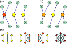
Figure 1: (a,b) For a quantum network of eight parties, two possible network configurations are shown: (a) two two-qubit sources and one four-qubit source and (b) one two-qubit source and two three-qubit sources are used to distribute eight qubits. In this paper, we design and implement an efficient method to discriminate these and all other configurations. (c) For the experimental implementation, we consider a six-qubit network, where four different configurations shall be distinguished. Here, the sources distribute two-, four- or six-qubit GHZ states, which are depicted by the fully connected graphs.

In all aforementioned cases, the characterization of the distributed entanglement across the network is indispensable. So far, however, the tools with which this goal can be achieved have been limited mainly to analyzing which quantum states and correlations can and cannot be established in a given network structure [15, 16, 17, 18, 19, 20, 21]. In order to understand the properties and limitations of a given quantum network, however, it is crucial to certify its topology. This refers to the probing of a set of targeted quantum network configurations (see Fig. 1) and goes beyond the characterization of single distributed quantum states [20, 22, 23]. First approaches to this problem have recently been given [24, 25]. But, although the proposed methods can distinguish between certain topologies, they assume the distribution of pure states or specific noise models and do not allow for certifying the quantum nature of the distributed states.

Conceptually speaking, the scenario of topology certification amounts to the joint test of several mutually exclusive hypotheses. This is significantly different from many existing works in quantum information science, where typically only one hypothesis is compared with one null hypothesis [26, 27, 28, 29, 30]. We also add that the related problem of community detection in classical networks has been intensively discussed [31, 32, 33], but these approaches do not directly translate to a quantum mechanical formulation.

In this work, we explore in theory and experiment the resource-efficient hypothesis testing of distinct quantum network configurations. For this purpose, we devise and implement a protocol that allows us to statistically certify (or falsify) which hypothesis is consistent with the multipartite quantum state of a network. Importantly, our different tests are based on a common set of local measurements and are easily implementable. In the experiment, we generate six-qubit quantum networks with different multipartite entanglement structures from a flexible, engineered source based on time-multiplexing and feed-forward; different network topologies correspond to different feed-forward sequences in the same physical source. Our measurements then allow us to determine the generated entanglement configuration with high confidence. Finally, we present methods for the topology certification of networks which can also be applied if some nodes are not trusted or some measurement devices are not certified.

II Statement of the Problem

The problem we consider is best explained by an example; see Fig. 1. Consider eight parties connected through a quantum network. Then, entanglement is distributed via the network across eight qubits. As depicted in Fig. 1, this may be done in different ways: In network (a), the entanglement is distributed by two Bell pair sources together with one four-qubit source, whereas network (b) consists of one Bell pair and two three-qubit sources. Clearly, other topologies are also possible yet omitted here for the sake of clarity and simplicity. Here and in the following, we always assume that the sources distribute (potentially noisy) Greenberger-Horne-Zeilinger (GHZ) states,

$$\ket{GHZ_{n}}=\frac{1}{\sqrt{2}}(\ket{0}^{\otimes n}+\ket{1}^{\otimes n}),$$ (1)

consisting of $n$ qubits. For the two-qubit case, GHZ states are simply the maximally entangled Bell states. For more particles, they are also, in some sense, maximally entangled [34], and form valuable resources for multiparticle cryptography [4, 35] and quantum metrology [36, 37]. The key questions are now: How can the eight parties identify, in a simple manner, which of the different configurations the network qubits are currently sharing? How can they find out which types of sources have been used (e.g., how many qubits were entangled) and between which of their qubits entanglement has successfully been generated?

These questions, with appropriate modifications, arise in several situations. For instance, it may be that the parties are connected via an intricate network of qubits, where the network provider promises to generate maximally entangled states in different configurations. In this case, the parties may be interested in verifying the provider’s claims with minimum effort. Alternatively, consider a network with some dishonest participants. Then, some other participants may want to certify that they share an entangled state, while ensuring that this state is not shared with any potentially malicious party.

In the general case, the problem can be considered for $N$ nodes, corresponding to $N$ qubits from different sources. The aim is then to certify the topology of the network from which the qubits originate. Here, one may additionally assume that only GHZ states of maximally $M<N$ qubits can be generated by the sources, effectively reducing the set of possible configurations. In the following, we present an efficient scheme to measure all fidelities $F_{I}=\mathrm{tr}(\ket{GHZ_{I}}\bra{GHZ_{I}}\varrho_{I})$ for all possible configurations in a unified manner. The index $I$ denotes here the set of $|I|=n$ qubits on which the fidelity depends, and the state $\varrho_{I}$ is the reduced state on the qubits labeled by $I$; in Fig. 1(a), the set $I$ could be $\{1,2,3,4\}$, $\{5,6\}$ or $\{7,8\}$. This now allows us to derive statistically rigorous tests for the different hypotheses about the topology directly from the measurement data. Our approach can be formulated for well-characterized measurements on the qubits as well as for the device-independent scenario, where some parties are not trusted and the measurements are potentially misaligned. We stress that our approach is fundamentally different from the task of state discrimination for a set of states [38] as we are not assuming that the quantum state comes from a fixed collection of states. In addition, we do not make any assumptions about the kind of noise.

III Simultaneous fidelity estimation and hypothesis testing

To start, we recall how the fidelity of an $N$-qubit GHZ state can be determined [39]. This state can be decomposed into a diagonal term $\mathcal{D}_{N}$ and an anti-diagonal term $\mathcal{A}_{N}$, i.e.,

$$\outerproduct{GHZ_{N}}{GHZ_{N}}= \frac{1}{2}\big{(}\outerproduct{0}{0}^{\otimes N}+\outerproduct{1}{1}^{\otimes N}+\ket{0}\!\!\bra{1}^{\otimes N}$$

$$+\ket{1}\!\!\bra{0}^{\otimes N}\big{)}=\frac{1}{2}(\mathcal{D}_{N}+\mathcal{A}_{N}).$$ (2)

The diagonal term can be determined by performing the Pauli measurement $\sigma_{z}^{\otimes N}$ on all qubits. Concerning the anti-diagonal term, it has been shown that it can be written as $\mathcal{A}_{N}=\nicefrac{{1}}{{N}}\sum_{k=0}^{N-1}(-1)^{k}\mathcal{M}_{k}^{\otimes N}$, where the observables $\mathcal{M}_{k}$ are given by measurements in the $x$-$y$ plane of the Bloch sphere,

$$\mathcal{M}_{k}=\Big{[}\cos\left(\frac{k\pi}{N}\right)\sigma_{x}+\sin\left(\frac{k\pi}{N}\right)\sigma_{y}\Big{]}.$$ (3)

This means that the fidelity of an $N$-qubit GHZ state can be determined by in total $N+1$ local measurements. Note that the measurements $\mathcal{M}_{k}$ also depend on the number $N$ of qubits.

The key observation in our approach is that the decomposition of $\mathcal{A}_{N}$ is not unique. Indeed, other sets of measurements in the $x$-$y$ plane of the Bloch sphere also allow us to determine $\mathcal{A}_{N}$, as long as the measurements form a basis in the space of operators spanned by products of $\sigma_{x}$ and $\sigma_{y}$, with an even number of $\sigma_{y}$ [39]. This paves the way for the simultaneous estimation of several GHZ fidelities: From the measurement data of $\mathcal{M}_{k}^{\otimes N}$, $\mathcal{A}_{N}$ can be determined using the formula above. Furthermore, for any subset of $m<N$ qubits, the expectation values $\langle\mathcal{M}_{k}^{\otimes m}\rangle$ can be obtained from the same set of data, which allows for the computation of the fidelity of the $m$-qubit GHZ states with respect to the reduced state on these $m$ particles. Explicit formulas for the $m$-qubit fidelities are provided in Appendix A.

Combining the above observations leads to the following scheme for testing the topology of a network: For a given $N$, the parties perform the $N+1$ local measurements $\sigma_{z}^{\otimes N}$ and $\mathcal{M}_{k}^{\otimes N}$. They then use this data to determine the set of fidelities $\{F_{I}\}$ for each considered network configuration. This allows them to identify the actual configuration and, at the same time, to characterize the quality of the sources. If the parties know that the sources are at most $M$-partite, then it suffices to perform the $M$ measurements $\mathcal{M}_{k}^{\otimes N}$ with angles $\nicefrac{{k\pi}}{{M}}$ in the $x$-$y$ plane and the measurement $\sigma_{z}^{\otimes N}$.

It remains to discuss how to formulate a proper hypothesis test in the space of potential fidelities that can be used to make a decision based on the observed data. Here, the task is to formulate a set of exclusive hypotheses which correspond to the different topologies, are physically motivated, and, at the same time, allow for a direct estimation of a $p$-value. The $p$-value of a hypothesis describes the probability of observing the experimental data given that the hypothesis $H$ holds true, i.e., $p=\Pr[\mathrm{data}\mid H]$. From a physical point of view, it is important to certify that a working source delivers GHZ states with a fidelity $F>1/2$, as this guarantees the presence of genuine multiparticle entanglement [40, 41]. Moreover, there are intricate dependencies between the fidelities of different GHZ states. If a state on $n$ qubits has a high GHZ fidelity, then the reduced state on a subset of $m<n$ qubits has also a non-vanishing fidelity with a GHZ state (with potentially adjusted phases); indeed, we have $F_{m}>F_{n}/2$ because of the common entries on the diagonal.

The above considerations motivate the following strategy to formulate exclusive hypotheses in the space of all fidelities. Any topology $T$ is characterized by a set of fidelities $\{F^{T}_{I}\}$ of the included GHZ states. The hypothesis corresponding to $T$ is then given by a set of conditions of the type

$$F_{I}^{T}-\max_{G\supset I}\Big{\{}F_{G}^{T}\Big{\}}>\frac{1}{2},$$ (4)

where ${G\supset I}$ denotes the relevant supersets of the qubits in the $n$-qubit set ${I}$. For instance, in order to distinguish the distinct topologies in Fig. 1, the hypothesis for configuration (a) should contain the conditions $F_{\{1,2,3,4\}}>1/2$, $F_{\{5,6\}}>1/2$ and $F_{\{7,8\}}-F_{\{6,7,8\}}>1/2$, and the hypothesis for (b) the conditions $F_{\{1,2,3\}}-F_{\{1,2,3,4\}}>1/2$, $F_{\{4,5\}}>1/2$ and $F_{\{6,7,8\}}>1/2$, rendering these hypotheses mutually exclusive. Taking the differences of the fidelities, e.g., $F_{\{7,8\}}-F_{\{6,7,8\}}>1/2$, is necessary to distinguish between tripartite entanglement on $\{6,7,8\}$, which leads to high fidelities $F_{\{7,8\}}$ and $F_{\{6,7,8\}}$, and bipartite entanglement on $\{7,8\}$, which only results in a high fidelity $F_{\{7,8\}}$. Finally, one always has to consider the null hypothesis, where the fidelities are small, making it impossible to certify the network structure. Given such hypotheses, the $p$-values can directly be calculated from the data, using large deviation bounds, like the Hoeffding inequality; see also Appendix B and C for details.

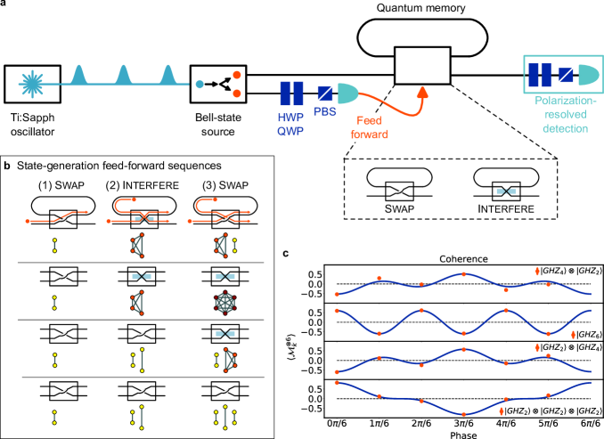
Figure 2: Operation principle of the experiment. (a) A dispersion-engineered, integrated Bell-state source probabilistically generates polarization-entangled Bell states. A successful polarization-resolved detection of one pair-photon generates a feed-forward signal to the quantum memory that stores its sibling. Retrieved light from the memory is detected in another polarization-resolved detection stage. The zoom-out shows the two operation modes of the memory: swap stores a new photon while releasing a stored photon without them interacting; interfere realizes a balanced interference between a new photon and a stored photon to increase the size of the entangled state. HWP: half-wave plate; QWP: quarter-wave plate; PBS: polarizing beam splitter. (b) Depending on the desired final network topology, different feed-forward sequences are implemented, which exchange swap and interfere operations of the quantum memory. Lines 2-4 show a smaller version of the quantum memory pictogram. (c) Measured average coherence terms $\langle\mathcal{M}_{k}^{\otimes 6}\rangle$ for the four different network topologies (orange markers), in the same order as in (b). The terms show an oscillatory dependence on the phase, which correlates with the number of entangled photons in each state. The blue lines are theory and serve as guide to the eye. Error bars are smaller than the symbol size.

IV Experimental generation of network states

The experimental implementation of our scheme demands a flexible state-generation circuit for the different entanglement configurations; see also Fig. 2 (a). We generate polarization-entangled Bell states with a dispersion-engineered parametric down-conversion source in a periodically poled potassium titanyl waveguide [42]. Larger entangled states are created with the help of a polarization qubit memory, based on an all-optical storage loop, which doubles as time-multiplexing device to increase generation rates and beam splitter to interfere successive Bell pairs [43]. The qubit memory’s operation mode—swap or interfere—is triggered by fast feed-forward based on the detection of one qubit from each Bell pair. We can generate four- and six-photon GHZ states with our setup at increased rates. Here, we make use of the specific programming capabilities of our system to generate four different six-photon states by changing the feed-forward sequence of the memory, without any physical changes in the experimental setup in practice; see Fig. 2 (b).

The first line schematically depicts the feed-forward sequence for the generation of a $|GHZ_{4}\rangle\otimes|GHZ_{2}\rangle$ network topology. Upon detection of a photon from the first Bell pair, its partner is stored in the memory by means of a swap operation. It is then interfered with a photon from the successive Bell pair to generate a $|GHZ_{4}\rangle$ state by means of the interfere operation. The stored photon is then exchanged for a photon from the third Bell pair via another swap operation. Note that we did not depict a final swap operation, which serves to read out the final photon from the memory. The interfere operation is essentially a fusion of two polarization qubits from two Bell pairs by interfering them on a polarizing beam splitter and post-selecting on a specific measurement pattern to create a graph state [44, 45].

Two consecutive interfere operations generate a $|GHZ_{6}\rangle$ state, while a swap operation followed by an interfere operation generates the state $|GHZ_{2}\rangle\otimes|GHZ_{4}\rangle$. Finally, two swap operations yield the state $|GHZ_{2}\rangle\otimes|GHZ_{2}\rangle\otimes|GHZ_{2}\rangle$, where photons from each Bell pair only share entanglement with each other. Note that in our setup fixing the phase of the six-photon GHZ state as $\ket{GHZ_{6}}=(\ket{0}^{\otimes 6}+\ket{1}^{\otimes 6})/{\sqrt{2}}$ implicitly fixes the phase of the four-photon state to $\ket{GHZ_{4}^{-}}=(\ket{0}^{\otimes 4}-\ket{1}^{\otimes 4})/{\sqrt{2}}$, so we formulate the hypotheses for this four-photon source.

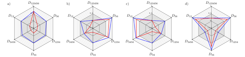
Figure 3: Graphical depiction of the fidelities (blue curves) and the differences of the fidelities considered in the hypotheses (red curves) for the four different measured datasets. The different directions $D_{I}$ denote either the fidelity $F_{I}$ (blue) or the difference $F_{I}-\max_{G\supset I}F_{G}$ (red). The differences allow for a clear separation between the states in the sense that only the desired terms are larger than $1/2$ (outside the dark area). The hypothesis test leads to the following results: dataset a) belongs to the state $\ket{GHZ_{6}}$, b) to $\ket{GHZ_{4}}\otimes\ket{GHZ_{2}}$, c) to $\ket{GHZ_{2}}\otimes\ket{GHZ_{4}}$ and d) to $\ket{GHZ_{2}}\otimes\ket{GHZ_{2}}\otimes\ket{GHZ_{2}}$.

Our source generates Bell states with entanglement visibility exceeding 93%. In total, we multiplex up to seven pump pulses to create the three Bell states required for this work. This yields a final six-photon event rate of approximately $0.3\,$Hz; more details are given in Appendix D. Note that higher rates can be achieved by multiplexing more pump pulses [43]. This, however, comes at the cost of a decreased state fidelity. As described above, for any network topology we perform the Pauli measurement $\sigma_{z}^{\otimes 6}$ as well as the measurements of the $\mathcal{M}_{k}^{\otimes 6}$. For the latter, we set the corresponding wave plate angles in front of the detection; see Fig. 2. We record around thousand successful events for every measurement setting to ensure good statistics. Our data yields H/V populations of $\mathcal{D}_{6}=(74\pm 1.7)\%$ and a total coherence value of $\mathcal{A}_{6}=(60\pm 0.9)\%$, resulting in a total fidelity of $F_{6}=0.67\pm 0.01$ for the $|GHZ_{6}\rangle$ state [46]. A plot of all coherence terms for the different topologies is shown in Fig. 2(c).

V Statistical model selection

All that remains to be done is the formulation of exclusive hypotheses and the calculation of the according $p$-values for our specific experiment. Naturally, we look for four distinct hypotheses according to the four possible configurations, and a fifth null hypothesis, which accounts for the case that none of the desired states was prepared. To exploit the fact that a fidelity higher than $1/2$ guarantees the presence of multipartite entanglement, it is reasonable to start with the hypothesis $H_{1}\ :\ F_{\{1,2,3,4,5,6\}}>1/2$, which describes the successful detection of a $6$-particle GHZ state. The next hypothesis $H_{2}$ responsible for the certification of the generation of $\ket{GHZ_{4}}\otimes\ket{GHZ_{2}}$ consists of two parts for the respective $GHZ$ states: $F_{\{1,2,3,4\}}-F_{\{1,2,3,4,5,6\}}>1/2$ and $F_{\{5,6\}}-\max\{F_{\{3,4,5,6\}},F_{\{1,2,3,4,5,6\}}\}>1/2$. The hypothesis $H_{3}$ and $H_{4}$, associated with the states $\ket{GHZ_{2}}\otimes\ket{GHZ_{4}}$ and $\ket{GHZ_{2}}\otimes\ket{GHZ_{2}}\otimes\ket{GHZ_{2}}$, respectively, are constructed in the same fashion and given explicitly in Appendix C. In Fig. 3, the different measured fidelities for the four different states are depicted together with the differences of the fidelities considered in the hypotheses.

The $p$-values of the hypotheses are given by the probability to observe the experimental data given that the respective hypothesis $H_{i}$ holds true, i.e., $p=\Pr[\mathrm{data}\mid H_{i}]$. The data in our case is given by the differences of the fidelities we compute, e.g., $d_{\{5,6\}}=F_{\{5,6\}}-\max\{F_{\{3,4,5,6\}},F_{\{1,2,3,4,5,6\}}\}$. We resort to calculating an upper bound on $p$, using the Hoeffding inequality [47] as in Refs. [26, 48]. The Hoeffding inequality is a large deviation bound for a sum of independent and bounded random variables. It states that the probability for this sum to differ from the mean value by a certain amount decreases exponentially in the number of variables. The measured difference of fidelities can be seen as a sum of the measurement results from the runs of the experiment, weighted with certain coefficients. Each measurement result in turn is an independent random event which can be modeled as a random variable so that we can apply Hoeffding’s inequality to the sum of these variables to bound the $p$-value. An exact analytical presentation of this bound and its proof can be found in Appendix C.

For each of the four generated states, we computed upper bounds on the $p$-values corresponding to the five hypotheses $H_{i}$ ($i=0,\dots,4$). The upper bounds concerning the null hypothesis are smaller than $9.5\times 10^{-8}$ for all states, i.e., the probability that the fidelities are too small to certify one of the network states is at most $9.5\times 10^{-8}$. For the four hypotheses $H_{1}$, $H_{2}$, $H_{3}$ and $H_{4}$, there exists one hypothesis for each state, for which the $p$-value is trivially upper bounded by one, while the other three $p$-values are upper bounded by at most $1.2\times 10^{-32}$. The exact values of the bounds are given in Table 1 of Appendix C.

VI Device-independent approach

So far, we have assumed that the performed measurements are well calibrated and that the nodes are trusted. This, however, may not necessarily be the case. The key to discussing the device-independent scenario is to consider the Bell operator from the Mermin inequality [49], which reads for three particles as

$$\mathcal{B}_{3}=X\otimes X\otimes X-X\otimes Y\otimes Y-Y\otimes X\otimes Y-Y\otimes Y\otimes X.$$ (5)

Here, $X$ and $Y$ are general dichotomic observables, but not necessarily Pauli matrices. For local realistic models, $\langle\mathcal{B}_{3}\rangle\leq 2$ has to hold while the GHZ state reaches $\langle\mathcal{B}_{3}\rangle=4$ if the measurements $X=\sigma_{x}$ and $Y=\sigma_{y}$ are performed. The Mermin inequality can be generalized to more particles; it consists of a combination of $X$ and $Y$ measurements with an even number of $Y$s and alternating signs. Formally, this can efficiently be written as $\mathcal{B}_{N}=[(X+iY)^{\otimes N}+(X-iY)^{\otimes N}]/2$, and, with the identification $X=\sigma_{x},Y=\sigma_{y}$, one finds $\mathcal{B}_{N}=2^{N}\mathcal{A}_{N}$.

The essential point is that several results connecting the expectation value $\langle\mathcal{B}_{N}\rangle$ with the GHZ-state fidelity are known. First, if nothing is assumed about the measurements, and if the value $\langle\mathcal{B}_{N}\rangle$ is close to the algebraic maximum $2^{N}$, a high GHZ fidelity up to some local rotations is certified [50]. Second, as we show in Appendix E, if one assumes that $X$ and $Y$ are (potentially misaligned) measurements on qubits, one can directly formulate a lower bound on the GHZ fidelity. Third, it has been shown that, even in the presence of collaborating dishonest nodes, the global state must be close to a GHZ state if the honest nodes choose $X=\sigma_{x}$ and $Y=\sigma_{y}$ as measurements [20]. Finally, if all parties choose $X=\sigma_{x}$ and $Y=\sigma_{y}$, then $F_{N}\geq\langle\mathcal{B}_{N}\rangle/2^{N}$ since for quantum states $\langle\mathcal{D}_{N}\rangle\geq\langle\mathcal{A}_{N}\rangle$.

The above comments suggest the following scheme for the device independent scenario. All parties measure all combinations of $X$ and $Y$, leading to $2^{N}$ measurements in total. Then, they can evaluate the Bell operator of the Mermin inequality on each subset and characterize the fidelity for all sources with three or more qubits, depending on the assumptions they can justify. For the case that the maximal size of the GHZ states is known to be $M<N$, not all $2^{N}$ measurements need to be performed. Rather, a smartly chosen subset of these measurements suffices as the scheme of overlapping tomography allows to evaluate all combinations of $X$ and $Y$ on $M$-particle subsets with an effort increasing only logarithmically in $M$ [51]. Finally, one may also consider advanced measurement schemes based on continuous stabilizers [21], or the Svetlichny inequality [22], which may be more efficient in the presence of dishonest parties.

VII Discussion

We devised and directly realized a resource-efficient scheme for probing the entanglement topology of quantum networks. Our method is based on a small set of local measurements, is easily implementable and scalable, and can be generalized to the device-independent scenario. Employing our flexibly programmable experimental setup based on feed-forward and time multiplexing, we were able to generate six-photon, polarization-encoded qubit states with different multipartite entanglement structures and discriminate them with high confidence.

Our work opens an avenue to several new research directions in the field of quantum information science. First, our methods can be extended to characterize other network scenarios. For instance, other quantum states besides GHZ states, such as cluster and graph states [52, 53], may be distributed and certified. Also, one may include the effects of classical communication, imperfect quantum memories, and probabilistic entanglement generation to certify the topology of the classical and quantum layer of a network. Second, our approach is an example of a multiple hypothesis test, a concept which has natural applications to other problems. An example is the joint estimation of several incompatible measurements [54] from simpler ones. Here, also shadow-like techniques based on randomized measurements may be a fruitful tool [55].

VIII Appendix A: Coefficients for the fidelity calculation

Given an $N$-qubit GHZ-state, it is known as mentioned in the main text that its fidelity $F_{N}=\Tr{\varrho\ket{GHZ_{N}}\bra{GHZ_{N}}}$ with some state $\varrho$ can be obtained by measuring $N+1$ different measurement settings only [39]. These consist of the Pauli-$Z$ measurement $\sigma_{z}^{\otimes N}$ and the $N$ measurements

$$\mathcal{M}_{k}^{\otimes N}=\left[\cos\left(\frac{k\pi}{N}\right)\sigma_{x}+\sin\left(\frac{k\pi}{N}\right)\sigma_{y}\right]^{\otimes N},\quad k=0,\dots,N-1.$$ (6)

Since these are all local measurements, all measurement results of $\sigma_{z}^{\otimes n}$ and $\mathcal{M}_{k}^{\otimes n}$ for $n\leq N$ can be deduced from the same measurement data. We now show that, by using the results of these measurements, we can also compute the fidelity of any $n$-qubit reduced state of $\varrho$ (denoted $\varrho^{(n)}$) with an $n$-party GHZ-state for $n<N$. For simplicity, we just write $F_{n}$ for this fidelity and omit the notation on which $n$ parties the fidelity is calculated.

First, we note that the $GHZ_{n}$ state can be written as

$$\ket{GHZ_{n}}\bra{GHZ_{n}}=\frac{1}{2}\left(\ket{0}\bra{0}^{\otimes n}+\ket{1}\bra{1}^{\otimes n}\right)+\frac{1}{2}\left(\ket{0}\bra{1}^{\otimes n}+\ket{1}\bra{0}^{\otimes n}\right)=:\frac{1}{2}(\mathcal{D}_{n}+\mathcal{A}_{n})$$ (7)

such that the fidelity $F_{n}$ reads as

$$F_{n}=\Tr(\varrho\ket{GHZ_{n}}\bra{GHZ_{n}}\otimes\mathds{1}_{N-n})=\frac{1}{2}\left[\Tr(\varrho^{(n)}\mathcal{D}_{n})+\Tr(\varrho^{(n)}\mathcal{A}_{n})\right].$$ (8)

The expectation values of $\ket{0}\bra{0}^{\otimes n}$ and $\ket{1}\bra{1}^{\otimes n}$, and thus of $\mathcal{D}_{n}$, can be directly recovered from the measurement results of $\sigma_{z}^{\otimes N}$ for all $n\leq N$. The calculation of the expectation value of $\mathcal{A}_{n}$ is not as trivial, and we show that there exist real coefficients $a_{k}$ ($k=0,\dots,N-1$) such that

$$\sum_{k=0}^{N-1}a_{k}\mathcal{M}_{k}^{\otimes n}=\mathcal{A}_{n}.$$ (9)

This means that the expectation value of $\mathcal{A}_{n}$ can be obtained from the measurement results of $\mathcal{M}_{k}^{\otimes n}$. Note that the fidelity of $\varrho$ with the $\ket{GHZ_{n}^{-}}$ state, which is given by

$$\ket{GHZ_{n}^{-}}=\frac{1}{\sqrt{2}}(\ket{0}^{\otimes n}-\ket{1}^{\otimes n}),$$ (10)

can also be calculated directly from the same data by just switching the sign from $\mathcal{A}_{n}$ to $-\mathcal{A}_{n}$.

Theorem 1.

The $N$-dimensional vector of coefficients $\vec{a}$ in Eq. (9) is given by

$$\vec{a}={\mathrm{diag}}(e^{-i\pi\frac{kn}{N}})\mathcal{F}^{-1}(\vec{c}),$$ (11)

where ${\mathrm{diag}}(e^{-i\pi\frac{kn}{N}})$ denotes the diagonal matrix with entries $e^{-i\pi\frac{kn}{N}}$ ($k=0,\dots,N-1$) and $\mathcal{F}^{-1}$ denotes the inverse discrete Fourier transform (DFT) of $\vec{c}=(1,0,\dots,0,1,c_{n+1},\dots,c_{N-1})\in\mathbb{C}^{N}$.

Proof.

Let us first rewrite $\mathcal{M}_{k}$ as

$$\mathcal{M}_{k} =\cos\left(\frac{k\pi}{N}\right)\left[\ket{0}\bra{1}+\ket{1}\bra{0}\right]+\sin\left(\frac{k\pi}{N}\right)\left[-i\ket{0}\bra{1}+i\ket{1}\bra{0}\right]$$ (12)

$$=e^{-i\frac{k\pi}{N}}\ket{0}\bra{1}+e^{i\frac{k\pi}{N}}\ket{1}\bra{0},\quad k=0,\dots,N-1,$$ (13)

and thus

$$\sum_{k=0}^{N-1}a_{k}\mathcal{M}_{k}^{\otimes n} =\sum_{j=0}^{n}\left[\sum_{k=0}^{N-1}e^{-i\pi\frac{k}{N}j}e^{i\pi\frac{k}{N}(n-j)}a_{k}\right]\sum_{\pi}\left[\bigotimes_{l=0}^{j}\ket{0}\bra{1}\bigotimes_{l=j+1}^{n}\ket{1}\bra{0}\right]$$ (14)

$$=:\sum_{j=0}^{n}c_{j}\sum_{\pi}\left[\bigotimes_{l=0}^{j}\ket{0}\bra{1}\bigotimes_{l=j+1}^{n}\ket{1}\bra{0}\right],$$ (15)

where $\sum_{\pi}\dots$ denotes the sum over all permutations leading to different terms. It now follows directly that we must have $c_{0}=c_{n}=1$ and $c_{2}=\dots=c_{n-1}=0$ with

$$c_{j}=\sum_{k=0}^{N-1}e^{-i\pi\frac{k}{N}j}e^{i\pi\frac{k}{N}(n-j)}a_{k}=\sum_{k=0}^{N-1}e^{-2\pi i\frac{kj}{N}}e^{i\pi\frac{kn}{N}}a_{k}$$ (16)

for $j=0,\dots,n$. These are the first $n+1$ entries of the DFT of ${\mathrm{diag}}(e^{i\pi\frac{kn}{N}})\vec{a}$. By defining $c_{n+1},\dots,c_{N-1}$ through Eq. (16), we can consider the extended vector $\vec{c}=(1,0,\dots,0,1,c_{n+1},\dots,c_{N-1})$ as the entire DFT $\vec{c}=\mathcal{F}({\mathrm{diag}}(e^{i\pi\frac{kn}{N}})\vec{a})$. Using the inverse of the DFT, we arrive at

$$\vec{a}={\mathrm{diag}}(e^{-i\pi\frac{kn}{N}})\mathcal{F}^{-1}(\vec{c}),$$ (17)

or, alternatively,

$$a_{k}=\frac{1}{N}e^{-i\pi\frac{kn}{N}}\sum_{j=0}^{N-1}e^{2\pi i\frac{kj}{N}}c_{j},$$ (18)

with $c_{n+1},\dots,c_{N-1}\in\mathbb{C}$. ∎

Note that the coefficients $a_{k}$ are not necessarily real for an arbitrary choice of $c_{n+1},\dots,c_{N-1}$. In that case, one can simply take the real part $\mathrm{Re}(\vec{a})$ only without affecting the validity of Eq. (9) as $\mathcal{M}_{k}$ and $\mathcal{A}_{n}$ are hermitian. However, we show in the following Corollary that, from requiring a minimal norm of the coefficients $\norm{\vec{a}}_{2}$, it already follows that the vector $\vec{a}$ is real-valued. We will see in the following Appendix B that minimizing the norm $\norm{\vec{a}}_{2}$ leads to the best bounds on the accuracy of our fidelity estimate.

For the next part, we recall that $\norm{\mathcal{F}(\vec{a})}_{2}^{2}=N\norm{\vec{a}}_{2}^{2}$ holds true in the case of the DFT. Since $\vec{c}$ is the DFT of $\vec{a}$, up to a complex phase, it directly follows that $\norm{\vec{c}}_{2}^{2}=N\norm{\vec{a}}_{2}^{2}$. Keeping this in mind, we can directly calculate the coefficients $a_{k}$ with minimal norm $\norm{\vec{a}}_{2}$ from the above Theorem.

Corollary 2.

The coefficients $a_{k}$ minimizing the norm $\norm{\vec{a}}_{2}$ for fixed $n$ and $N$ are given by

$$a_{k}=\frac{1}{N}\begin{cases}(-1)^{k}\ &\text{for }n=N,\\ 2\cos(\pi\frac{kn}{N})\ &\text{for }n<N.\end{cases}$$ (19)

Proof.

Since the vectors $\vec{a}$ and $\vec{c}$ fulfill $\norm{\vec{c}}_{2}^{2}=N\norm{\vec{a}}_{2}^{2}$, the norm of $\vec{a}$ is minimal if and only if the norm of $\vec{c}$ is minimal. According to Theorem 1, the norm of the vector $\vec{c}$ reads as

$$\norm{\vec{c}}_{2}^{2}=1+0+\dots+0+1+|c_{n+1}|^{2}+\dots+|c_{N-1}|^{2},$$ (20)

which is minimal for $c_{n+1}=\dots=c_{N-1}=0$. Thus, the ideal choice for the vector $\vec{c}$ only contains up to two entries equal to one and has therefore a norm of $\norm{\vec{c}}_{2}=\sqrt{2}$ for $n<N$ and $\norm{\vec{c}}_{2}=1$ for $n=N$. In the case of $n<N$, this leads to

$$Na_{k}=e^{-i\pi\frac{kn}{N}}\left[e^{0}+e^{2\pi i\frac{kn}{N}}\right]=e^{-i\pi\frac{kn}{N}}+e^{\pi i\frac{kn}{N}}=2\cos(\pi\frac{kn}{N})$$ (21)

and, in the case of $n=N$, to

$$Na_{k}=e^{-i\pi\frac{kN}{N}}=e^{-i\pi k}=(-1)^{k},$$ (22)

which proves the statement. ∎

Note that in the case $n=N$ these are exactly the coefficients given in the main text. It follows directly from the above Corollary that the norm of the minimal coefficient vector $\vec{a}$ only depends on the number of qubits $\norm{\vec{a}}_{2}^{2}=\frac{1}{N}\norm{c}_{2}^{2}\leq\frac{2}{N}$. We will use this result in Appendix B to characterize the accuracy of the fidelities obtained from the experimental data.

IX Appendix B: Confidence region for fidelity estimation

In the asymptotic limit, the experimental data for a measurement $M$ ought to reproduce exactly the expectation value $\langle M\rangle$. However, since every experiment is restricted to a finite number of measurements, one can only calculate estimates of the expectation values from the measurement results. Here we describe a way to bound the accuracy of the calculated estimate using Hoeffding’s inequality [26, 47].

The setting is the following: We want to calculate the fidelity $F$, which is a linear combination of some observables $M_{i}$,

$$F=\sum_{i=0}^{N}d_{i}\langle M_{i}\rangle.$$ (23)

In our case, the coefficients and measurements will be the same as described in Appendix A. For now, however, we will look at the general case described above. In the experiment, each of the measurements $M_{i}$ will be measured for a finite number $m_{i}$ where each of these single measurements leads to a measurement result $A_{ij}$ ($j=1,\dots,m_{i}$). For example, measuring $m_{i}=10$ times the measurement $M_{i}=\sigma_{z}$ leads to the ten measurement results $A_{ij}=+1$ or $A_{ij}=-1$ for $j=1,\dots,10$. The estimate for the expectation value of $M_{i}$ is then calculated by

$$\widehat{\langle M_{i}\rangle}=\frac{1}{m_{i}}\sum_{j=1}^{m_{i}}A_{ij},$$ (24)

and the estimate for the fidelity $F$ is obtained accordingly by

$$\hat{F}=\sum_{i=0}^{N}d_{i}\widehat{\langle M_{i}\rangle}=\sum_{i=0}^{N}\frac{d_{i}}{m_{i}}\sum_{j=1}^{m_{i}}A_{ij}.$$ (25)

We now want to characterize the accuracy of this estimate by using Hoeffding’s inequality [47], which we briefly recall:

Lemma 3 (Hoeffding’s inequality [47]).

Let $X_{1},\dots,X_{m}$ be independent, bounded random variables such that there exist $s_{i}$ and $t_{i}$ with $s_{i}\leq X_{i}\leq t_{i}$. Then, the sum $S_{n}=\sum_{i=1}^{n}X_{i}$ fulfills

$$\Pr[(S_{n}-\langle S_{n})\rangle>\epsilon]<\exp{-\frac{2\epsilon}{C}},$$ (26)

with $C=\sum_{i=1}^{m}(t_{i}-s_{i})^{2}$.

For a proof, see [47].

Using this, we can now calculate the accuracy of the estimate $\hat{F}$.

Lemma 4.

Defining the fidelities, coefficients, and measurements in the same way as in Appendix A, and denoting the minimal number of measurements by $\mu=\min_{i}(m_{i})$, the estimate of the fidelity $\hat{F}$ obeys $\Pr[(\hat{F}_{n}-F_{n})>\epsilon]<\delta$ for $\delta(\epsilon)=\exp{-\frac{8\mu\epsilon^{2}}{1+8/N}}\Leftrightarrow\epsilon(\delta)=\sqrt{-\frac{1+8/N}{8\mu}\ln{\delta}}$.

Proof.

Following the notation in Appendix A, the fidelity reads

$$F_{n}=\sum_{k=0}^{N-1}\frac{a_{k}}{2}\langle\mathcal{M}_{k}^{\otimes n}\rangle+\frac{1}{2}\langle\mathcal{D}_{n}\rangle=:\sum_{k=0}^{N}\frac{a_{k}}{2}\langle M_{k}\rangle,$$ (27)

for $M_{k}=\mathcal{M}_{k}^{\otimes n}$ for $k=0,\dots,N-1$, $M_{N}=\mathcal{D}_{n}$ and $a_{N}=1$. Note that each measurement $M_{k}$ has only two possible measurement results: the measurements $\mathcal{M}_{k}^{\otimes n}$ can only result in either $+1$ or $-1$, and the measurement $\mathcal{D}_{n}$ only in either $0$ or $1$. Denoting the number of times each measurement $M_{i}$ is performed by $m_{i}$, and the result of the $j$-th measurement of $M_{i}$ by $A_{ij}$, the estimate of the fidelity is then

$$\hat{F}_{n}=\sum_{i=0}^{N}\frac{a_{i}}{2m_{i}}\sum_{j=1}^{m_{i}}A_{ij}.$$ (28)

Note that this is a sum of the independent random variables $\frac{a_{i}}{2m_{i}}A_{ij}$, whose expectation value yields the true fidelity,

$$\langle\hat{F}_{n}\rangle=\sum_{i=0}^{N}\frac{a_{i}}{2m_{i}}\sum_{j=1}^{m_{i}}\langle A_{ij}\rangle=\sum_{i=0}^{N}\frac{a_{i}}{2m_{i}}\sum_{j=1}^{m_{i}}\langle M_{i}\rangle=\sum_{i=0}^{N}\frac{a_{i}}{2}\langle M_{i}\rangle=F_{n}.$$ (29)

The random variables $A_{ij}$ themselves can only take two different values; for $i=N$, it holds

$$\frac{a_{N}}{2m_{N}}A_{Nj}\in\left\{\frac{a_{N}}{2m_{N}}\times 0,\frac{a_{N}}{2m_{N}}\times 1\right\}=\left\{0,\frac{1}{2m_{N}}\right\}$$ (30)

and, for $i=0,\dots,N-1$,

$$\frac{a_{i}}{2m_{i}}A_{ij}\in\left\{\frac{a_{i}}{2m_{i}}\times(-1),\frac{a_{i}}{2m_{i}}\times 1\right\}.$$ (31)

Using Hoeffding’s inequality, we therefore arrive at

$$\Pr[\left(\hat{F}_{n}-F_{n}\right)>\epsilon]=\Pr(\hat{F}_{n}-\langle\hat{F}_{n}\rangle>\epsilon)\leq\exp{-\frac{2\epsilon^{2}}{C}}$$ (32)

with

$$C =\sum_{i=0}^{N-1}\sum_{j=1}^{m_{i}}\left(\frac{a_{i}}{2m_{i}}-\frac{-a_{i}}{2m_{i}}\right)^{2}+\sum_{j=1}^{m_{N}}\left(\frac{1}{2m_{N}}\right)^{2}$$ (33)

$$=\sum_{i=0}^{N-1}\frac{a_{i}^{2}}{m_{i}}+\frac{1}{4m_{N}}$$ (34)

$$\leq\frac{1}{4\mu}\left(4\norm{\vec{a}}_{2}^{2}+1\right)$$ (35)

$$\leq\frac{1}{4\mu}\left(8/N+1\right),$$ (36)

which proves the statement. ∎

The last inequality follows directly from Corollary 2 and explains the need to minimize the norm of the coefficient vector $\vec{a}$.

In Appendix C, we want to test hypotheses which compare fidelities on different subsets. Let us for now denote two of these different fidelities by $F_{1}$ and $F_{2}$. Then, we can bound in exactly the same way as described above the probability by

$$\Pr[(\hat{F}_{1}-\hat{F}_{2})-(F_{1}-F_{2})>\epsilon]<\exp{-\frac{2\epsilon^{2}\mu}{1+8/N}}.$$ (37)

Intuitively, the factor of $4$ in the constant $C$ appears because the length of the intervals in which the summed random variables assume their values approximately doubles. Mathematically, the random variables $\frac{a^{(1)}_{i}}{2m_{i}}A^{(1)}_{ij}-\frac{a^{(2)}_{i}}{2m_{i}}A^{(2)}_{ij}$ arising in the calculation of the fidelity can now take four values, which are bounded by sums of the different coefficients $a^{(k)}_{i}$. Using the subadditivity of the norm $\norm{\cdot}_{2}$ in the calculation of the constant $C$ yields then the expression given above.

X Appendix C: Hypothesis testing

Recall that our goal is to distinguish between different topologies of distributed states. Using the calculated fidelities for subsets of $n$ of the $N$ qubits, we develop here a hypothesis test to decide which layout describes the measured data best. We do that by first formulating the different topologies as partitions of the set of all qubits. Then, we derive a hypothesis test for different partitions and calculate the $p$-value of each hypothesis using the results from Appendix B.

We start by noticing that the different layouts of a network can be seen as different partitions of the set $\{1,\dots,N\}$. We recall that a partition $P$ of $\{1,\dots,N\}$ is a set of subsets $\{I_{1},\dots,I_{k}\}$ of $\{1,\dots,N\}$ such that $I_{i}\neq\emptyset$ and $I_{i}\cap I_{j}=\emptyset$ for all $i,j$ and the union of all subsets covers again $\{1,\dots,N\}$,

$$\bigcup_{j=1}^{k}I_{j}=\{1,\dots,N\}.$$ (38)

For instance, the configurations (a) and (b) from Fig. 1 would correspond to the partitions $P_{a}=\{\{1,2,3,4\},\{5,6\},\{7,8\}\}$ and $P_{b}=\{\{1,2,3\},\{4,5\},\{6,7,8\}\}$, respectively.

As seen in the section before, all the fidelities $F_{n}=\Tr{\varrho\ket{GHZ_{n}}\bra{GHZ_{n}}\otimes\mathds{1}_{N-n}}$ for $n\leq N$ can be computed from only $N+1$ measurements. We now refine the notation to keep track on which $n$ parties the fidelity is calculated. We denote the $n$-party GHZ-state on the $n$ qubits $I\subseteq\{1,\dots,N\}$, $|I|=n$, by $\ket{GHZ_{I}}$ and the respective fidelity by $F_{I}=\Tr{\varrho\ket{GHZ_{I}}\bra{GHZ_{I}}\otimes\mathds{1}_{\overline{I}}}$. The overline $\overline{I}$ denotes the complement of $I$ in $\{1,\dots,N\}$.

Now, let $\mathcal{P}(\{1,\dots,N\})$ be the set of all partitions of $\{1,\dots,N\}$. Physically, we interpret a given partition $P=\{I_{1},\dots,I_{k}\}$ as the subsets of parties $I_{j}$ on which a GHZ-state was distributed. This means we expect the global state of the network to be

$$\bigotimes_{j=1}^{k}\ket{GHZ_{I_{j}}}\bra{GHZ_{I_{j}}}=\bigotimes_{I\in P}\ket{GHZ_{I}}\bra{GHZ_{I}}.$$ (39)

In our case, we have $N=6$ photons which can be entangled in four different ways:

$$\ket{\Psi_{1}}= \ket{GHZ_{6}},$$ (40a)

$$\ket{\Psi_{2}}= \ket{GHZ_{4}}\otimes\ket{GHZ_{2}},$$ (40b)

$$\ket{\Psi_{3}}= \ket{GHZ_{2}}\otimes\ket{GHZ_{4}},\quad\mathrm{and}$$ (40c)

$$\ket{\Psi_{4}}= \ket{GHZ_{2}}\otimes\ket{GHZ_{2}}\otimes\ket{GHZ_{2}}.$$ (40d)

These four cases correspond to the four partitions

$$P_{1}= \{\{1,2,3,4,5,6\}\},$$ (41a)

$$P_{2}= \{\{1,2,3,4\},\{5,6\}\},$$ (41b)

$$P_{3}= \{\{1,2\},\{3,4,5,6\}\},\quad\mathrm{and}$$ (41c)

$$P_{4}= \{\{1,2\},\{3,4\},\{5,6\}\},$$ (41d)

respectively. To discriminate these different possible configurations from the measured data, we now develop a hypothesis test in which the hypotheses exclude each other, ensuring that only one hypothesis can be accepted.

Lemma 5.

Let $P_{1},\dots,P_{K}\in\mathcal{P}(\{1,\dots,N\})$ be $K$ different partitions such that for every pair of partitions $P_{i}$ and $P_{j}$, there exists at least one subset in each partition $\tilde{I}\in P_{i}$ and $\tilde{J}\in P_{j}$ with $\tilde{I}\subsetneq\tilde{J}$ or $\tilde{I}\supsetneq\tilde{J}$. Then, the $K+1$ hypotheses $H_{1},\dots,H_{K}$ and $H_{\emptyset}$ given by

$$H_{i}\ :\ \forall I\in P_{i}\ :\ F_{I}-\max_{G\supset I}F_{G}>\frac{1}{2}\quad\forall i\in\{1,\dots,K\},$$ (42)

$$H_{\emptyset}\ :\ \mathrm{otherwise}$$ (43)

are pairwise exclusive to each other, i.e. only one of them can be accepted.

Proof.

Clearly, the different hypotheses $H_{i}$ and the hypothesis $H_{\emptyset}$ are mutually exclusive by definition. So, it is only left to show that any two hypotheses $H_{i}$ and $H_{j}$, with $i\neq j$, exclude each other. From the assumptions, there exist two sets $\tilde{I}\in P_{i}$ and $\tilde{J}\in P_{j}$ which fulfill without loss of generality $\tilde{I}\subsetneq\tilde{J}$. Let us now assume that both hypotheses could be accepted at the same time. It follows that

$$F_{\tilde{I}} >\frac{1}{2}+\max_{G\supset\tilde{I}}F_{G}\geq\frac{1}{2}+F_{\tilde{J}}\quad\mathrm{and}$$ (44)

$$F_{\tilde{J}} >\frac{1}{2}+\max_{G\supset\tilde{J}}F_{G}\geq\frac{1}{2}.$$ (45)

But then we have

$$F_{\tilde{I}}>\frac{1}{2}+F_{\tilde{J}}>\frac{1}{2}+\frac{1}{2}=1,$$ (46)

which contradicts the fact that fidelities can be at most one, i.e. $F_{\tilde{I}}\leq 1$, and completes the proof. ∎

The different partitions of Eq. (41) obviously fulfill the condition in Lemma 5. So, in our case, we have the five following different hypotheses:

$$H_{1}\ :\ F_{123456}>\nicefrac{{1}}{{2}};$$ (47a)

$$H_{2}\ :\ \begin{cases}h_{21}\ &:\ F_{1234}-F_{123456}>\nicefrac{{1}}{{2}}\quad\mathrm{and}\\ h_{22}\ &:\ F_{56}-\max\{F_{3456},F_{123456}\}>\nicefrac{{1}}{{2}};\\ \end{cases}$$ (47b)

$$H_{3}\ :\ \begin{cases}h_{31}\ &:\ F_{12}-\max\{F_{1234},F_{123456}\}>\nicefrac{{1}}{{2}}\quad\mathrm{and}\\ h_{32}\ &:\ F_{3456}-F_{123456}>\nicefrac{{1}}{{2}};\end{cases}$$ (47c)

$$H_{4}\ :\ \begin{cases}h_{41}\ &:\ F_{12}-\max\{F_{1234},F_{123456}\}>\nicefrac{{1}}{{2}},\\ h_{42}\ &:\ F_{34}-\max\{F_{1234},F_{3456},F_{123456}\}>\nicefrac{{1}}{{2}}\quad\mathrm{and}\\ h_{43}\ &:\ F_{56}-\max\{F_{3456},F_{123456}\}>\nicefrac{{1}}{{2}},\\ \end{cases}$$ (47d)

and

$$H_{\emptyset}\ :\ \text{otherwise},$$ (47e)

respectively. Note that, for the sake of simplicity, we wrote, e.g., $12$ for the set $\{1,2\}$.

So, if we have the true fidelities $F_{I}$ on every one of these specific subsets, we can unambiguously decide which hypothesis or configuration is true and reject the other possibilities. However, as we only have access to finite statistics, and therefore to estimates of the fidelities, we now have to calculate the $p$-values of every single hypothesis. The $p$-value describes the probability to get a certain experimental result, in our case the calculated estimate of the fidelity, given that a hypothesis is true.

Since the hypotheses $H_{i}$ of Eq. (42) are all of the same form, we concentrate on a single one of these, consisting of $m$ terms of the type $F_{I}-\max_{J\supset I}F_{J}>\frac{1}{2}$. For the sake of readability, we neglect the index $I$ in the following calculations and denote the hypothesis by $H$, consisting of the sub-hypotheses $h_{i}\ :\ F^{(i)}-\max_{J}F^{(i)}_{J}>\frac{1}{2}$ ($i=1,\dots,k$). Additionally, we introduce the shorthand notation $X^{(i)}_{J}:=F^{(i)}-F^{(i)}_{J}$, or equivalently $\min_{J}X^{(i)}_{J}:=F^{(i)}-\max_{J}F^{(i)}_{J}$. With this notation, the $p$-value of the hypothesis for the minimum of the estimates

$$d_{i}:=\min_{J}\widehat{X^{(i)}_{J}},$$ (48)

which are calculated from the experimentally observed data, reads as

$$p=\Pr[\min_{J}\widehat{X^{(i)}_{J}}\leq d_{i}\ \forall i\in\{1,\dots,k\}\mid H].$$ (49)

First, we prove a short and later helpful Lemma.

Lemma 6.

With the notation introduced above and the fidelities defined as in Appendix A and B, it holds

$$\Pr[\left(\min_{J}\widehat{X^{(i)}_{J}}-\min_{J}X^{(i)}_{J}\right)>\epsilon]\leq\exp{-\frac{2\epsilon^{2}\mu}{1+8/N}}.$$ (50)

Proof.

To be able to use the results from Appendix B, we note that the minimum $\min^{(i)}_{J}X^{(i)}_{J}=:X^{(i)}_{\tilde{J}}$ is assumed for at least one $\tilde{J}$. Additionally, the probability for the minimum of the estimates $\min_{J}\widehat{X^{(i)}_{J}}$ being larger than some value is upper bounded by the probability for any of the $\widehat{X^{(i)}_{J}}$ to be larger than that same value. We therefore arrive at

$$\Pr[\left(\min_{J}\widehat{X^{(i)}_{J}}-\min_{J}X^{(i)}_{J}\right)>\epsilon]=\Pr[\left(\min_{J}\widehat{X^{(i)}_{J}}-X^{(i)}_{\tilde{J}}\right)>\epsilon]\leq\Pr[\left(\widehat{X^{(i)}_{\tilde{J}}}-X^{(i)}_{\tilde{J}}\right)>\epsilon]\overset{\eqref{eq:estFidelity}}{\leq}\exp{-\frac{2\epsilon^{2}\mu}{1+8/N}}=\delta(\epsilon),$$ (51)

with $\epsilon=\sqrt{-\frac{1+8/N}{2\mu}\ln(\delta)}$. ∎

Now, since it is not possible to calculate the $p$-value exactly given that it only compares fidelities, we provide an upper bound for the $p$-value.

Lemma 7.

For the hypothesis $H$ described above, the $p$-value in Eq. (49) is bounded by

$$p\leq\delta(d)$$ (52)

where $d$ and $\delta(d)$ are defined by $d=\min\{d_{1},\dots,d_{k},1/2\}$ and $\delta(d)=\exp{-\frac{2(1/2-d)^{2}M}{1+8/N}}$.

Proof.

We use the fact that the random variables $\min_{J}X_{J}^{(i)}$ and their estimates are resulting from quantum states $\varrho$. We define regions in the state space where the different hypotheses are fulfilled,

$$R_{i}:= \{\varrho\mid h_{i}\ :\ \min_{J}X_{J}^{(i)}>\nicefrac{{1}}{{2}}\ \mathrm{is\ true}\},\quad i\in\{1,\dots,k\}\quad\mathrm{and}$$ (53)

$$R:= \{\varrho\mid h_{i}\ :\ \min_{J}X_{J}^{(i)}>\nicefrac{{1}}{{2}}\ \mathrm{is\ true}\ \forall i\in\{1,\dots,k\}\}.$$ (54)

Obviously, it holds $R\subseteq R_{i}$. We now can calculate a bound on the $p$-value by maximizing over the possible quantum states which lie in $R$:

$$p =\Pr[\min_{J}\widehat{X^{(j)}_{J}}\leq d_{j}\ \forall j\mid H]\leq\max_{\varrho\in R}\Pr[\min_{J}\widehat{X^{(j)}_{J}}\leq d_{j}\ \forall j\mid\varrho]\leq\max_{\varrho\in R_{i}}\Pr[\min_{J}\widehat{X^{(j)}_{J}}\leq d_{j}\ \forall j\mid\varrho]\quad\forall i.$$ (55)

Since this holds for every $R_{i}$, it also holds for the minimum over $i$. Additionally, the joint probability for the different events $\min_{J}\widehat{X^{(j)}_{J}}\leq d_{j}$ is bounded by the probability of one of these events. We therefore arrive at

$$p \leq\min_{i}\max_{\varrho\in R_{i}}\Pr[\min_{J}\widehat{X^{(j)}_{J}}\leq d_{j}\ \forall j\mid\varrho]\leq\min_{i}\max_{\varrho\in R_{i}}\Pr[\min_{J}\widehat{X^{(i)}_{J}}\leq d_{i}\mid\varrho].$$ (56)

However, the probability in the last line can be bounded using Lemma 6. Indeed, for the case $d_{i}<1/2$, it holds

$$\max_{\varrho\in R_{i}}\Pr[\min_{J}\widehat{X^{(i)}_{J}}\leq d_{i}\mid\varrho] \leq\Pr[\left(\min_{J}X_{J}^{(i)}-\min_{J}\widehat{X^{(i)}_{J}}\right)\geq 1/2-d_{i}]$$ (57)

$$\overset{\eqref{eq:probMin}}{\leq}\exp{-\frac{2(1/2-d_{i})^{2}\mu}{1+8/N}}=:\delta(d_{i}).$$ (58)

For the case $d_{i}\geq 1/2$, however, we only obtain the trivial bound

$$\max_{\varrho\in R_{i}}\Pr[\min_{J}\widehat{X^{(i)}_{J}}\leq d_{i}\mid\varrho]\leq 1=\delta(1/2).$$ (59)

Since $\delta(d_{i})$ decreases for decreasing $d_{i}<1/2$, we get

$$p \leq\min_{i}\max_{\varrho\in R_{i}}\Pr[\min_{J}\widehat{X^{(i)}_{J}}\leq d_{i}\mid\varrho]\leq\delta(\min\{d_{1},\dots,d_{k},1/2\}),$$ (60)

which concludes the proof. ∎

The intuition behind this proof is that the probability for the observed data given the hypothesis $H$ is upper bounded by the probability of the least probable event. Since the hypothesis $H$ consists of statements of the type $d_{i}>1/2$ the least probable result $d_{i}$ is the one farthest away from $1/2$, namely $\min_{i}d_{i}<1/2$.

The only hypothesis which cannot be described in the above manner is the null hypothesis $H_{\emptyset}$ in Lemma 5. However, this hypothesis can be written as

$$H_{\emptyset}\ :\ \forall i\in\{1,\dots,K\}\ \exists I^{(i)}\in P_{i}\ :\ \min_{G}(F_{I^{(i)}}-F_{G})\leq 1/2.$$ (61)

For a fixed combination of the sets $I^{(i)}$, we can argue in the same way as in Lemma 7: the probability for the calculated estimates is bounded by

$$\Pr[\min_{G}(\widehat{F_{I^{(i)}}}-\widehat{F_{G}})\geq d_{i}\mid\min_{G}(F_{I^{(i)}}-F_{G})\leq 1/2]\leq\begin{cases}\delta(d_{i})&\text{for }d_{i}>1/2,\\ 1&\text{else},\end{cases}$$ (62)

with $\delta(d_{i})=\exp{-\frac{2(1/2-d_{i})^{2}M}{1+8/N}}$. Thus, we have

$$\Pr[\min_{G}(\widehat{F_{I^{(j)}}}-\widehat{F_{G}})\geq d_{j}\ \forall j\mid H_{\emptyset}]\leq\min_{j}\{\delta(d_{j}),1\}.$$ (63)

The $p$-value itself is then bounded by the maximum over the different combinations of the $I^{(i)}$

$$p \leq\max_{\{I^{(i)}\}}\Pr[\min_{G}(\widehat{F_{I^{(i)}}}-\widehat{F_{G}})\geq d_{i}\ \forall i\mid H_{\emptyset}]$$ (64)

$$\leq\max_{\{I^{(i)}\}}\min_{i}\{\delta(d_{i}),1\}$$ (65)

$$\leq\min\{\delta(d),1\},$$ (66)

where $d=\min_{\{i\mid d_{i}>1/2\}}d_{i}$.

Intuitively, this can again be understood in the following way: The probability for the observed data given the hypothesis $H_{\emptyset}$ is upper bounded by the probability of the least probable event. The least probable event in this case is the one farthest away from $1/2$, namely $\max_{i}d_{i}>1/2$. Since the exact combination of the $I^{(i)}$ and therefore the $d_{i}$ one has to consider in the maximization are unknown, one can only upper bound the $p$-value by the worst case $d_{i}$, namely the one nearest to but still larger than $1/2$; that is $d=\min_{\{i\mid d_{i}>1/2\}}d_{i}$.

Table 1: Upper bound on the $p$-value of the different hypotheses for the four different states. We recall that the hypotheses are explicitly given in Eq. (47), and that $H_{1}$ corresponds to $F_{123456}$ being large, $H_{2}$ to $F_{1234}$ and $F_{56}$ being large, $H_{3}$ to $F_{12}$ and $F_{3456}$ being large, $H_{4}$ to $F_{12}$, $F_{34}$ and $F_{56}$ being large and, finally, $H_{\emptyset}$ is the null hypothesis.

	$H_{1}$	$H_{2}$	$H_{3}$	$H_{4}$	$H_{\emptyset}$
Dataset 1	$1$	$2.3724\times 10^{-139}$	$9.2153\times 10^{-146}$	$3.0256\times 10^{-116}$	$9.4765\times 10^{-8}$
Dataset 2	$8.3274\times 10^{-92}$	$1$	$1.6231\times 10^{-258}$	$1.6231\times 10^{-258}$	$1.4347\times 10^{-13}$
Dataset 3	$6.1789\times 10^{-93}$	$6.8294\times 10^{-259}$	$1$	$8.8629\times 10^{-272}$	$1.3010\times 10^{-23}$
Dataset 4	$1.1810\times 10^{-32}$	$3.7960\times 10^{-174}$	$4.9169\times 10^{-188}$	$1$	$2.3295\times 10^{-22}$

XI Appendix D: Additional data and experimental details

An in-depth description and characterization of our experiment can be found in Ref. [43]. A dispersion-engineered, spectrally decorrelated guided-wave parametric down-conversion in a periodically poled potassium titanyl waveguide is pumped with ultrafast pump pulses with a central wavelength of $\lambda_{p}=775\,$nm. The source is arranged in a Sagnac configuration to generate polarization-entangled Bell states with a central wavelength of $\lambda_{\mathrm{Bell}}=1550\,$nm [42]. A set of tomographic wave plates (half-wave plate, quarter-wave plate) and a polarizing beam splitter are used in one arm of the source to implement a polarization-resolving heralding measurement. We use superconducting nanowire single-photon detectors with an efficiency of more than 70% and recovery time of $11\,$ns for photon detection. These allow to operate the source at the full laser repetition rate of $76\,$MHz, corresponding to a time difference between successive laser pulses of $13.6\,$ns. A successful heralding detection event is fed forward to a high-speed electro-optic switch inside the quantum memory. The switch is, effectively, a Pockels cell that rotates the polarization of an incoming light pulse when a high voltage is applied. It has a response time (rise and/or fall time) of less than $5\,$ns. Depending on when the switching occurs, we can realize the swap and interfere operations described in the main text. Again, more details are found in Ref. [43].

The quantum memory itself is an all-optical, free-space storage loop with a memory bandwidth beyond $1\,$THz, a memory efficiency of 91%, and a lifetime of $131\,$ns. Its operation state is controlled by a field-programmable gate array (FPGA), which converts the heralding detection events into switching time lists for the Pockels cell as well as a time gate for the photon detection behind the memory. The latency of the feed-forward is compensated for by sending the photons through a $300\,$m long single-mode fiber. After retrieval from the memory, photons are sent to another polarization-resolving detection stage. A successful datum is registered when six photons are detected in total, three herald photons in different time bins together with three photons from the memory in the corresponding time bins. Hence, a complete experiment consists of the following steps: Firstly, define the network topology and the corresponding switching sequence; secondly, perform a test measurement of the H/V populations to assess system performance; thirdly, measure all relevant observables by automatically setting the corresponding wave-plate angles and collecting data until a predetermined number of successful events (in our case around thousand) has been measured.

Figure 4 exemplarily shows the click-correlation matrices for the H/V populations of the four network topologies considered in the main text (top row) and the $\langle\mathcal{M}_{3}^{\otimes 6}\rangle$ coherence term (lower row). Note that the same data sets have been used to calculate the observables as described in the main text.

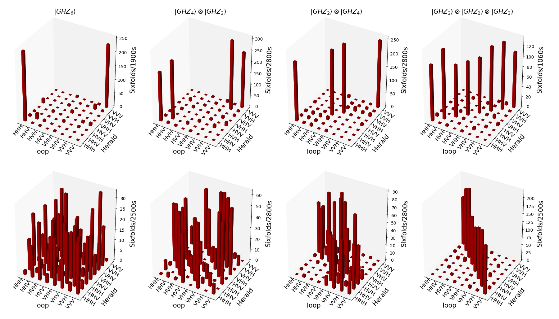
Figure 4: (Top row) Population of six-fold clicks for the four different topologies (as named in figure) measured in the H/V basis. Direct population analysis shows $\mathcal{D}_{N}$ values of $(74\pm 1.7)\%$, $(83.7\pm 1.1)\%$, $(82.3\pm 1.1)\%$, and $(92.6\pm 0.8)\%$, respectively, for the states from left to right. A Poissonian error on the counts is included in the data analysis. As expected, fidelities decrease for larger-size GHZ states. (Bottom row) Six-fold click probabilities measured in a specific coherence term ($\langle\mathcal{M}_{3}^{\otimes 6}\rangle$) setting.

XII Appendix E: Semi-Device-independent estimation on the fidelity

In a device-independent scenario, there are no assumptions made on the measurements. As mentioned in the main text, there are already results connecting the violation of a Mermin inequality by some state with its GHZ-state fidelity [50]. In the following, using the experimentally observed violation of the Mermin inequality $S_{N}=\expectationvalue{\mathcal{B}_{N}}$, we will give a lower bound of the GHZ-state fidelity under the assumption that one performs (misaligned) measurements $X$ and $Y$ on qubits.

Firstly, recall that the Bell operator of the Mermin inequality for $N$ qubits is given by

$$\mathcal{B}_{N}=[(X+iY)^{\otimes N}+(X-iY)^{\otimes N}]/2.$$ (67)

We then specify the observables as

$$X =\sigma_{x},$$ (68)

$$Y =\sin(\theta_{k})\sigma_{x}+\cos(\theta_{k})\sigma_{y},$$ (69)

where $\theta_{k}$ is the angle denoting the misalignment from a perfect measurement ($X=\sigma_{x}$ and $Y=\sigma_{y}$), which can be different for each qubit $k=1,...,N$. Note that we can assume $X=\sigma_{x}$ since we are only interested in the GHZ-state fidelity modulus local unitaries. For the same reason, it is no further restriction to assume the second measurement to be in the $x$-$y$ plane of the Bloch sphere.

The goal is now to estimate the lower bound on the GHZ-state fidelity, given a violation $S_{N}$ of the $N$-qubit Mermin inequality. For two qubits, this has previously been done using the spectral decomposition of the Clauser, Horne, Shimony, Holt (CHSH) operator [56]. We now extend this method to $N>2$ qubits by using the spectral decomposition of the Mermin operator $\mathcal{B}_{N}$ and the fact that, for any Bell operator with two observables per qubit, its eigenstates (if not degenerate) are given by the $N$-qubit GHZ states, such that its eigendecomposition is $\mathcal{B}_{N}=\sum_{i}\lambda_{i}\ket{GHZ_{i}}\bra{GHZ_{i}}$ [34].

The idea is now the following: If the violation exceeds a certain value $S_{N}$, we want to be able to state that the fidelity for some GHZ state $\ket{GHZ_{i}}$ is at least $F$. Thus, we start by fixing a fidelity $F$ and maximize the violation of the Bell inequality.

Consider the expectation value of the Bell operator for some state $\varrho$,

$$S_{N} =\Tr(\mathcal{B}_{N}\varrho)=\sum_{i}\lambda_{i}\bra{GHZ_{i}}\varrho\ket{GHZ_{i}}$$ (70)

$$=\sum_{i}\lambda_{i}F(\varrho,\ket{GHZ_{i}})\leq\lambda_{1}F+\lambda_{2}(1-F),$$ (71)

where we fixed the largest fidelity $F\coloneqq\max_{i}\{F(\varrho,\ket{GHZ_{i}})\}$ and sorted the eigenvalues $\lambda_{i}$ in decreasing order.

As mentioned before, the measurements might be misaligned with respect to some angles $\theta_{k}$ and therefore the eigenvalues $\lambda_{i}$ are functions of the angles $\theta_{k}$. Since we are interested in the largest violation one can achieve for a fixed fidelity $F$, we have to consider all possible misalignments $\{\theta_{k}\}$. Then, Eq. (71) reads

$$S_{N}\leq\max_{\{\theta_{k}\}}[\lambda_{1}(\{\theta_{k}\})F+\lambda_{2}(\{\theta_{k}\})(1-F)].$$ (72)

In order to find the maximum of this expression, consider

$$\mathcal{B}_{N}^{2}=[((X+iY)^{2})^{\otimes N}+((X-iY)^{2})^{\otimes N}+((X+iY)(X-iY))^{\otimes N}+((X-iY)(X+iY))^{\otimes N}]/4.$$ (73)

Using $\Tr(\sigma_{i}\sigma_{j})=2\delta_{ij}$, it follows that $\Tr(XY)=2\sin(\theta_{k})$, and further that

$$\Tr(\mathcal{B}_{N}^{2}) =[\prod_{k=1}^{N}4i\sin(\theta_{k})+\prod_{k=1}^{N}(-4i)\sin(\theta_{k})+4^{N}+4^{N}]/4$$ (74)

$$=[(4i)^{N}\prod_{k=1}^{N}\sin(\theta_{k})+(-4i)^{N}\prod_{k=1}^{N}\sin(\theta_{k})+2\cdot 4^{N}]/4.$$ (75)

For an odd number of qubits $N$, this reduces to

$$\Tr(\mathcal{B}_{N}^{2}) =[2\cdot 4^{N}]/4=2^{-1}2^{2N}=2^{N}2^{N-1}.$$ (76)

Following Ref. [34], where similar formulas were derived, we note that

$$\sum_{i=1}^{2^{N}}\lambda_{i}^{2}=\Tr(\mathcal{B}_{N}^{2})=2^{N}2^{N-1}.$$ (77)

Further, it is known that the eigenvalues of the Mermin operator $\mathcal{B}_{N}$ appear pairwise with alternating signs; therefore, summing up only the squared positive eigenvalues yields

$$\sum_{i=1}^{2^{N-1}}(\lambda_{i}^{+})^{2}=2^{N}2^{N-1}/2=2^{2(N-1)}.$$ (78)

Thus, the two largest eigenvalues must fulfill

$$\lambda_{1}^{2}+\lambda_{2}^{2}\leq 2^{2(N-1)}.$$ (79)

We can use this to parameterize $\lambda_{1}=2^{N-1}\cos(\alpha)$ and $\lambda_{2}=2^{N-1}\sin(\alpha)$, as done in Ref. [56]. Note that $\alpha$ is not directly connected to the misalignment $\theta_{k}$ anymore, but it simply represents a parameter used to express all possible configurations for $\lambda_{1}$ and $\lambda_{2}$ saturating Eq. (79). Then, Eq. (72) yields

$$S_{N} \leq\max_{\alpha}[2^{N-1}\cos(\alpha)F+2^{N-1}\sin(\alpha)(1-F)]$$ (80)

$$\leq 2^{N-1}\sqrt{F^{2}+(1-F)^{2}},$$ (81)

using that $\max_{\alpha}(a\sin(\alpha)+b\cos(\alpha))=\sqrt{a^{2}+b^{2}}$, and it follows that

$$F\geq\frac{1}{2}+\frac{1}{\sqrt{2}}\sqrt{\left(\frac{S_{N}}{2^{N-1}}\right)^{2}-\frac{1}{2}}$$ (82)

for an odd number of qubits. Note that this expression is only defined if the violation is large enough, which shows that, in the semi-device-independent scenario, a violation of at least $S_{N}=2^{N-1}/\sqrt{2}$ is needed to certify entanglement. Furthermore, if the maximal violation $2^{N-1}$ is achieved, the GHZ-state fidelity is $F=1$.

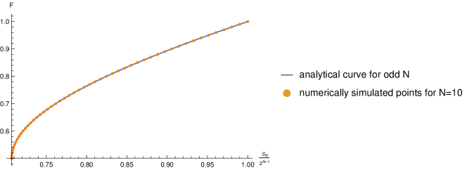
Figure 5: The minimum GHZ-state fidelity for a given violation of the $N$-qubit Mermin inequality. We compare the analytically computed curve following Eq. (82) to the numerically simulated values for 10 qubits.

Lastly, it is to mention that this ansatz to find the analytical expression only works for an odd number of qubits. However, when numerically maximizing Eq. (72) for up to 10 qubits and scaling the violation with a factor $2^{-(N-1)}$, we obtain the same curve for all $N$, as shown in Fig. 5. Thus, we conjecture that Eq. (82) is true for all $N$.

References

- Kimble [2008] H. J. Kimble, Nature 453, 1023 (2008).
- Wehner et al. [2018] S. Wehner, D. Elkouss, and R. Hanson, Science 362, 303 (2018).
- Azuma et al. [2022] K. Azuma, S. E. Economou, D. Elkouss, P. Hilaire, L. Jiang, H.-K. Lo, and I. Tzitrin, Quantum repeaters: From quantum networks to the quantum internet (2022), arXiv:2212.10820 [quant-ph] .
- Murta et al. [2020] G. Murta, F. Grasselli, H. Kampermann, and D. Bruß, Adv. Quantum Technol. 3, 2000025 (2020).
- Komar et al. [2014] P. Komar, E. M. Kessler, M. Bishof, L. Jiang, A. S. Sørensen, J. Ye, and M. D. Lukin, Nat. Phys. 10, 582 (2014).
- Sekatski et al. [2020] P. Sekatski, S. Wölk, and W. Dür, Phys. Rev. Res. 2, 023052 (2020).
- Proctor et al. [2018] T. J. Proctor, P. A. Knott, and J. A. Dunningham, Phys. Rev. Lett. 120, 080501 (2018).
- Barz et al. [2012] S. Barz, E. Kashefi, A. Broadbent, J. F. Fitzsimons, A. Zeilinger, and P. Walther, Science 335, 303 (2012).
- Hermans et al. [2022] S. L. N. Hermans, M. Pompili, H. K. C. Beukers, S. Baier, J. Borregaard, and R. Hanson, Nature 605, 663 (2022).
- Liu et al. [2023] J.-L. Liu, X.-Y. Luo, Y. Yu, C.-Y. Wang, B. Wang, Y. Hu, J. Li, M.-Y. Zheng, B. Yao, Z. Yan, D. Teng, J.-W. Jiang, X.-B. Liu, X.-P. Xie, J. Zhang, Q.-H. Mao, X. Jiang, Q. Zhang, X.-H. Bao, and J.-W. Pan, A multinode quantum network over a metropolitan area (2023), arXiv:2309.00221 [quant-ph] .
- Nitsche et al. [2020] T. Nitsche, S. De, S. Barkhofen, E. Meyer-Scott, J. Tiedau, J. Sperling, A. Gábris, I. Jex, and C. Silberhorn, Phys. Rev. Lett. 125, 213604 (2020).
- Collins et al. [2007] O. A. Collins, S. D. Jenkins, A. Kuzmich, and T. A. B. Kennedy, Phys. Rev. Lett. 98, 060502 (2007).
- Shchukin et al. [2019] E. Shchukin, F. Schmidt, and P. van Loock, Phys. Rev. A 100, 032322 (2019).
- Weinbrenner et al. [2023] L. T. Weinbrenner, L. Vandré, T. Coopmans, and O. Gühne, Aging and reliability of quantum networks (2023), arXiv:2305.19976 [quant-ph] .
- Navascues et al. [2020] M. Navascues, E. Wolfe, D. Rosset, and A. Pozas-Kerstjens, Phys. Rev. Lett. 125, 240505 (2020).
- Kraft et al. [2021] T. Kraft, S. Designolle, C. Ritz, N. Brunner, O. Gühne, and M. Huber, Phys. Rev. A 103, L060401 (2021).
- Luo [2021] M.-X. Luo, Adv. Quantum Technol. 4, 2000123 (2021).
- Tavakoli et al. [2022] A. Tavakoli, A. Pozas-Kerstjens, M.-X. Luo, and M.-O. Renou, Rep. Prog. Phys. 85, 056001 (2022).
- Hansenne et al. [2022] K. Hansenne, Z.-P. Xu, T. Kraft, and O. Gühne, Nat. Commun. 13, 496 (2022).
- Pappa et al. [2012] A. Pappa, A. Chailloux, S. Wehner, E. Diamanti, and I. Kerenidis, Phys. Rev. Lett. 108, 260502 (2012).
- McCutcheon et al. [2016] W. McCutcheon, A. Pappa, B. A. Bell, A. Mcmillan, A. Chailloux, T. Lawson, M. Mafu, D. Markham, E. Diamanti, I. Kerenidis, et al., Nat. Commun. 7, 13251 (2016).
- Murta and Baccari [2023] G. Murta and F. Baccari, Self-testing with dishonest parties and device-independent entanglement certification in quantum networks (2023), arXiv:2305.10587 [quant-ph] .
- Kao et al. [2023] W.-T. Kao, C.-Y. Huang, T.-J. Tsai, S.-H. Chen, S.-Y. Sun, Y.-C. Li, T.-L. Liao, C.-S. Chuu, H. Lu, and C.-M. Li, Scalable quantum network determination with Einstein-Podolsky-Rosen steering (2023), arXiv:2303.17771 [quant-ph] .
- Chen et al. [2023] D. T. Chen, B. Doolittle, J. M. Larson, Z. H. Saleem, and E. Chitambar, Inferring quantum network topology using local measurements (2023), arXiv:2212.07987 [quant-ph] .
- Yang et al. [2022] X. Yang, Y.-H. Yang, and M.-X. Luo, Phys. Rev. Res. 4, 013153 (2022).
- Flammia and Liu [2011] S. T. Flammia and Y.-K. Liu, Phys. Rev. Lett. 106, 230501 (2011).
- Yu et al. [2022] X.-D. Yu, J. Shang, and O. Gühne, Adv. Quantum Technol. 5, 2100126 (2022).
- Saggio et al. [2019] V. Saggio, A. Dimić, C. Greganti, L. A. Rozema, P. Walther, and B. Dakić, Nat. Phys. 15, 935 (2019).
- Pallister et al. [2018] S. Pallister, N. Linden, and A. Montanaro, Phys. Rev. Lett. 120, 170502 (2018).
- Martínez Vargas et al. [2021] E. Martínez Vargas, C. Hirche, G. Sentís, M. Skotiniotis, M. Carrizo, R. Muñoz Tapia, and J. Calsamiglia, Phys. Rev. Lett. 126, 180502 (2021).
- Newman [2018] M. Newman, Networks (Oxford University Press, 2018).
- Zachary [1977] W. W. Zachary, J. Anthropol. Res. 33, 452 (1977).
- Girvan and Newman [2002] M. Girvan and M. E. J. Newman, Proc. Natl. Acad. Sci. USA 99, 7821 (2002).
- Scarani and Gisin [2001] V. Scarani and N. Gisin, J. Phys. A Math. Gen. 34, 6043 (2001).
- Christandl and Wehner [2005] M. Christandl and S. Wehner, in Lecture Notes in Computer Science (Springer Berlin Heidelberg, 2005) pp. 217–235.
- Tóth and Apellaniz [2014] G. Tóth and I. Apellaniz, J. Phys. A Math. Theor. 47, 424006 (2014).
- Giovannetti et al. [2004] V. Giovannetti, S. Lloyd, and L. Maccone, Science 306, 1330 (2004).
- Barnett and Croke [2009] S. M. Barnett and S. Croke, Adv. Opt. Photonics 1, 238 (2009).
- Gühne et al. [2007] O. Gühne, C.-Y. Lu, W.-B. Gao, and J.-W. Pan, Phys. Rev. A 76, 030305 (2007).
- Gühne and Tóth [2009] O. Gühne and G. Tóth, Physics Reports 474, 1 (2009).
- Horodecki et al. [2009] R. Horodecki, P. Horodecki, M. Horodecki, and K. Horodecki, Rev. Mod. Phys. 81, 865 (2009).
- Meyer-Scott et al. [2018] E. Meyer-Scott, N. Prasannan, C. Eigner, V. Quiring, J. M. Donohue, S. Barkhofen, and C. Silberhorn, Opt. Express 26, 32475 (2018).
- Meyer-Scott et al. [2022] E. Meyer-Scott, N. Prasannan, I. Dhand, C. Eigner, V. Quiring, S. Barkhofen, B. Brecht, M. B. Plenio, and C. Silberhorn, Phys. Rev. Lett. 129, 150501 (2022).
- Bouwmeester et al. [1999] D. Bouwmeester, J.-W. Pan, M. Daniell, H. Weinfurter, and A. Zeilinger, Phys. Rev. Lett. 82, 1345 (1999).
- Lu et al. [2007] C.-Y. Lu, X.-Q. Zhou, O. Gühne, W.-B. Gao, J. Zhang, Z.-S. Yuan, A. Goebel, T. Yang, and J.-W. Pan, Nat. Phys. 3, 91 (2007).
- Wang et al. [2016] X.-L. Wang, L.-K. Chen, W. Li, H.-L. Huang, C. Liu, C. Chen, Y.-H. Luo, Z.-E. Su, D. Wu, Z.-D. Li, H. Lu, Y. Hu, X. Jiang, C.-Z. Peng, L. Li, N.-L. Liu, Y.-A. Chen, C.-Y. Lu, and J.-W. Pan, Phys. Rev. Lett. 117, 210502 (2016).
- Hoeffding [1963] W. Hoeffding, J. Am. Stat. Assoc. 58, 13 (1963).
- Moroder et al. [2013] T. Moroder, M. Kleinmann, P. Schindler, T. Monz, O. Gühne, and R. Blatt, Phys. Rev. Lett. 110, 180401 (2013).
- Mermin [1990] N. D. Mermin, Phys. Rev. Lett. 65, 1838 (1990).
- Kaniewski [2016] J. Kaniewski, Phys. Rev. Lett. 117, 070402 (2016).
- Cotler and Wilczek [2020] J. Cotler and F. Wilczek, Phys. Rev. Lett. 124, 100401 (2020).
- Meignant et al. [2019] C. Meignant, D. Markham, and F. Grosshans, Phys. Rev. A 100, 052333 (2019).
- Hahn et al. [2022] F. Hahn, A. Dahlberg, J. Eisert, and A. Pappa, Phys. Rev. A 106, L010401 (2022).
- Gühne et al. [2023] O. Gühne, E. Haapasalo, T. Kraft, J.-P. Pellonpää, and R. Uola, Rev. Mod. Phys. 95, 011003 (2023).
- Huang et al. [2020] H.-Y. Huang, R. Kueng, and J. Preskill, Nat. Phys. 16, 1050 (2020).
- Bardyn et al. [2009] C.-E. Bardyn, T. C. H. Liew, S. Massar, M. McKague, and V. Scarani, Phys. Rev. A 80, 062327 (2009).