EarnHFT: Efficient Hierarchical Reinforcement Learning for
High Frequency Trading

Abstract

High-frequency trading (HFT) uses computer algorithms to make trading decisions in short time scales (e.g., second-level), which is widely used in the Cryptocurrency (Crypto) market (e.g., Bitcoin). Reinforcement learning (RL) in financial research has shown stellar performance on many quantitative trading tasks. However, most methods focus on low-frequency trading, e.g., day-level, which cannot be directly applied to HFT because of two challenges. First, RL for HFT involves dealing with extremely long trajectories (e.g., 2.4 million steps per month), which is hard to optimize and evaluate. Second, the dramatic price fluctuations and market trend changes of Crypto make existing algorithms fail to maintain satisfactory performance. To tackle these challenges, we propose an Efficient hieArchical Reinforcement learNing method for High Frequency Trading (EarnHFT), a novel three-stage hierarchical RL framework for HFT. In stage I, we compute a Q-teacher, i.e., the optimal action value based on dynamic programming, for enhancing the performance and training efficiency of second-level RL agents. In stage II, we construct a pool of diverse RL agents for different market trends, distinguished by return rates, where hundreds of RL agents are trained with different preferences of return rates and only a tiny fraction of them will be selected into the pool based on their profitability. In stage III, we train a minute-level router which dynamically picks a second-level agent from the pool to achieve stable performance across different markets. Through extensive experiments in various market trends on Crypto markets in a high-fidelity simulation trading environment, we demonstrate that EarnHFT significantly outperforms 6 state-of-art baselines in 6 popular financial criteria, exceeding the runner-up by 30% in profitability.

1 Introduction

High-frequency trading (HFT), taking up more than 73% volume in the fincial market, refers to leveraging complicated computer algorithms or mathematical models to place or cancel orders at incredibly short time scales (Almeida and Gonçalves 2023). A good HFT strategy enables investors to make more profit than a low-frequency strategy and is therefore pursued by many radical traders. It has been widely used in Cryptocurrency (Crypto) market due to Crypto’s 24/7 non-stop trading time, which prevents Crypto holders from overnight risk, and dramatic price fluctuations, which provides more profitable trading opportunities for HFT.

Although reinforcement learning (RL) algorithms (Sun et al. 2022; Théate and Ernst 2021; Cumming, Alrajeh, and Dickens 2015) have achieved outstanding results in low-frequency trading in traditional financial markets like stock or futures, few maintain robust performance under the setting of HFT due to two challenges:

• An extremely large time horizon induces low data efficiency for RL training. Compared with Atari games where the time horizon is 6000 (Mnih et al. 2013), the time horizon of HFT is around 1 million, because second-level agents need to be evaluated in dozens of days. Large time horizons need more data to converge (Zhang et al. 2023a), demanding more computational resources.

• The dramatic market changes cause agents trained on history data to fail in maintaining performance over long periods. In a traditional RL setting, the training and testing environments remain consistent. However, Crypto market trend changes cause a significant difference between the training and testing environments. An agent trained on one market trend tends to cause tremendous losses once the trend changes dramatically in the market.

To tackle the challenges, we propose an Efficient hieArchical Reinforcement learNing method for High Frequency Trading (EarnHFT) as shown in Figure 1. In stage I, we build a Q-teacher indicating the optimal action value based on dynamic programming and future price information, which is used as a regularizer to train RL agents delivering a target position every second for better performance and faster training speed. In stage II, we first train hundreds of second-level RL agents following the stage I process under different market trend preferences, where buy and hold (Shiryaev 2008) return rates are used as the preference indicators. We further label each market based on DTW (Muda, Begam, and Elamvazuthi 2010) as different categories and use the profitability performance under each market category to select a tiny fraction of trained second-level RL agents to construct a strategy pool. In stage III, we train a router which dynamically picks a second-level agent from the pool per minute to achieve stable performance across different markets. Through extensive experiments in various market trends in the Crypto market under a high-fidelity simulation trading environment, we demonstrate that EarnHFT significantly outperforms 6 state-of-art baselines in terms of 6 popular financial criteria, exceeds the runner-up by at least 30% in terms of profitability.

2 Related Works

In this section, we introduce the related works on traditional finance methods used in HFT and RL for quantitative trading. More discussion can be found in Appendix A.

2.1 High-Frequency Trading in Crypto

HFT, aiming to profit from slight price fluctuation in a short period of time in the market, has been widely used in companies (Zhou et al. 2021). Crypto traders invest differently from those in stock markets because of the high volatility (Delfabbro, King, and Williams 2021). In the Crypto market, there are many high-frequency technical indicators (Huang, Huang, and Ni 2019), such as imbalance volume (IV) (Chordia, Roll, and Subrahmanyam 2002) and moving average convergence divergence (MACD) (Krug, Dobaj, and Macher 2022), to capture buying and selling pressures among different time scales. However, these technical indicators also have limitations. In the volatile Crypto market, technical indicators may produce false signals. The result is sensitive to hyper-parameter settings, e.g. the take profit point and the stop loss.

2.2 RL for Quantitative Trading

Many deep reinforcement learning methods for quantitative trading have been proposed. DeepScalper (Sun et al. 2022) uses a hindsight bonus and auxiliary task to improve the model’s generalization ability in intraday trading. DRA (Briola et al. 2021) uses LSTM and PPO. CDQNRP (Zhu and Zhu 2022) uses a random perturbation to increase the stability of training a convolution DQN. However, these algorithms focus mainly on designing only one powerful RL agent to conduct profitable trading in short-term scenarios, neglecting its failure of maintaining performance over long periods.

Hierarchical Reinforcement Learning (HRL), which decomposes a long-horizon task into a hierarchy of sub-problems, has been studied for decades. There are some hierarchical RL frameworks for quantitative trading. HRPM (Wang et al. 2021) utilizes a hierarchical framework to simulate portfolio management and order execution. MetaTrader (Niu, Li, and Li 2022) proposes a router to pick the most suitable strategy for the current market situation. However, these hierarchical frameworks are all utilized in portfolio management. Its application remains unexplored in HFT where only one asset is traded.

3 Problem Formulation

In this section, we present some basic finance concepts used in simulating the trading process and propose a hierarchical Markov decision process (MDP) framework for HFT.

3.1 Financial Foundations for HFT

We first introduce some basic financial concepts used to describe state, reward, and action in the following hierarchical Markov Decision Process (MDP) framework and present the objective of HFT.

Limit Order Book (LOB) records unfilled orders. It is widely used to describe the market micro-structure (Madhavan 2000) in finance. We denote an m-level LOB at time $t$ as $b_{t}=(p_{t}^{b_{1}},p_{t}^{a_{1}},q_{t}^{b_{1}},q_{t}^{a_{1}},...,p_{t}^{b_{m}},p_{t}^{a_{m}},q_{t}^{b_{m}},q_{t}^{a_{m}})$, where $p_{t}^{b_{i}}$ ($p_{t}^{a_{i}}$) is the level $i$ bid (ask) price, $q_{t}^{b_{i}}$ ($q_{t}^{a_{i}}$) is the quantity.

OHLC is aggregated information of executed orders. OHLC vector at time $t$ is denoted as $x_{t}=(p_{t}^{o},p_{t}^{h},p_{t}^{l},p_{t}^{c})$, where $p_{t}^{o},p_{t}^{h},p_{t}^{l},p_{t}^{c}$ indicate the open, high, low and close price.

Technical Indicators indicate features calculated by a formulaic combination of the original OHLC or LOB to uncover the underlying pattern of the financial market. We denote the technical indicator vector at time $t$ $y_{t}=\phi(b_{t},x_{t},...,b_{t-h},x_{t-h})$, where $\phi$ is the function that maps OHLC and LOB to technical indicators.

Market Order is a trade to buy or sell a financial asset instantly. The executed price is calculated as Equation 1.

$$E_{t}(M)=\sum_{i}(p_{t}^{i}\times\min(q_{t}^{i},R_{i-1}))(1+\sigma)$$ (1)

where $E$ is the execution price, $R_{i-1}$ is the remaining quantity after level $i$ in LOB, $\sigma$ is the commission fee rate, and $q_{t}^{i},p_{t}^{i}$ are the level $i$ price and quantity in LOB respectively.

Position is the amount of a financial asset traders hold. Position at time $t$ is denoted as $P_{t}$ and $P_{t}\geq 0$, indicating only a long position is permitted in this formulation.

Net Value $V_{t}$ is the sum of cash and value of the position, calculated as $V_{t}=V_{ct}+P_{t}\times p_{t}^{b1}$, where $V_{ct}$ is the cash.

We aim to maximize the net value by conducting market orders on a single asset based on market information (e.g., LOB and OHLC) at a second-level time scale.

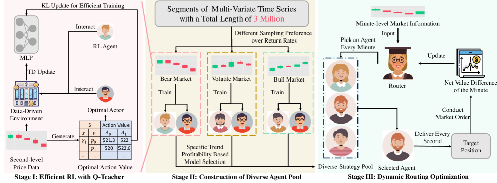
Figure 1: The overview of EarnHFT. First, we compute a Q-teacher for enhancing the performance and training efficiency of second-level RL agents. Then, we efficiently train diverse RL agents under various market trends and select a small fraction of them to form an agent pool based on profitability. Finally, we train a minute-level router which dynamically picks a second-level agent from the pool to achieve stable performance across different markets.

3.2 Hierarchical MDP Framework

In this subsection, we formulate HFT as a hierarchical MDP. An MDP is defined by the tuple: ($S$, $A$, $P$, $r$, $\gamma$, $T$), where $S$ is the state space and $A$ is the action space. $P:S\times A\times S\rightarrow[0,1]$ is the transition function, $r:S\times A\times S\rightarrow R$ is the reward function, $\gamma\in(0,1]$ is the discount factor and $T$ is the time horizon. In an MDP, the agent receives the current state $s_{t}\in S$ from the environment, performs an action $a_{t}\in A$, and gets the next state $s_{t+1}\in S$ and a reward $r_{t}$. An agent’s policy is defined by $\pi_{\theta}$ : $S\times A\rightarrow[0,1]$, which is parameterized by $\theta$. The objective of the agent is to learn an optimal policy $\pi^{*}=\arg\max_{\theta}E_{\pi_{\theta}}[\sum_{t=0}^{T}\gamma^{t}r_{t}|S_{0}]$ where $s_{0}$ is the initial state of the MDP.

In RL for HFT, data drifting of the micro-level market information prevents a single agent from maintaining its performance over long periods and it is difficult to train a profitable agent under all trends because of the conflict in effective strategies under different market conditions. Macro-level information, as an aggregation of micro-level market information, provides insight into the dynamics of the micro-level market. Therefore, we formulate HFT as a hierarchical MDP, where the low-level MDP operating on a second-level time scale formulates the process of micro-level market dynamics and trading execution and the high-level MDP operating on a minute-level time scale formulates the process of the macro-level market trends and strategy adjustment. It is defined by ($\text{MDP}_{h}$, $\text{MDP}_{l}$), where

$$\text{MDP}_{h} =(S_{h},A_{h},P_{h},R_{h},\gamma_{h},T_{h})$$

$$\text{MDP}_{l} =(S_{l},A_{l},P_{l},R_{l},\gamma_{l},T_{l})$$

Low-level State $S_{lt}$ at time $t$ consists of two parts: the latent representation $X_{lt}$, which is the micro-level market technical indicators and private state $P_{t}$. $X_{lt}$ consists of 54 features and is calculated as $X_{lt}=\phi_{l}(C_{lt})$ where $C_{lt}$ is a rolling window of second-level OHLC and the snapshot of LOB with length 60. $P_{t}$ indicates the current position of the agent.

Low-level Action $a_{lt}$ at time $t$ is the target position. It is chosen from a predefined position pool $A_{l}$ with finite elements defined as $\{0,\frac{H}{|A|-1},...,H\}$ where $|A|$ represents the number of the action choices and $H$ is the maximum position. If $a_{lt}\neq P_{t}$, then we instantly take a market order $E_{t}(a_{lt}-P_{t})$, making the current position to $a_{lt}$.

Low-level Reward $r_{lt}$ at time $t$ is the net value differential in the second-level time scale, referring to money made through one second. It is calculated as $r_{lt}=P_{t+1}\times p_{t+1}^{b1}-(P_{t}\times p_{t}^{b1}+E_{t}(P_{t+1}-P_{t})$, where we use the best bid price to calculate the value of the current position.

High-level State $S_{ht}$ at time $t$ also consists of two parts: the latent representation $X_{ht}$, which is the macro-level market technical indicators and private state $P_{t}$. $X_{ht}$ consists of 19 features and is calculated as $X_{ht}=\phi_{h}(C_{ht})$ where $C_{ht}$ is a rolling window of minute-level OHLC length 60. $P_{t}$ indicates the current position of the agent.

High-level Action $a_{ht}$ is the selected agent at time $t$. It is chosen from a pre-trained agent pool $A_{h}$, each of which is trained under a low-level MDP.

High-level Reward $r_{lt}$ at time $t$ is the net value differential in the minute-level time scale, referring to money made through one minute. It is also the return of the selected low-level agent makes under low-level MDP in one minute and is calculated as $r_{hT}=\sum_{t=T}^{T+\tau}r_{lt}$.

In this bilevel hierarchical MDP framework, for every minute, our high-level agent picks a low-level agent, which will adjust its position every second to make profit. We aim to find a set of low-level agents (traders) and a high-level agent (router) to maximize our total profit.

4 EarnHFT

In this section, we demonstrate three stages of EarnHFT as shown in Figure 1. In stage I, we present RL with Q-teacher, which improves the training efficiency, to train low-level agents. In stage II, agents are trained and evaluated in different market trends, forming a diverse pool for hierarchical constructions. In stage III, we train a router to pick a proper agent to maintain profitability in the non-stationary market.

4.1 Stage I: Efficient RL with Q-Teacher

A long trajectory causes extra computational cost in traditional RL settings. However, in our low-level MDP, the price information is not influenced by our policy. By using future price information and dynamic programming, we can easily construct the optimal action value (Sutton and Barto 2018) to help train RL agents more efficiently. Here, we use an optimal value supervisor and an optimal actor to aid training.

Optimal Value Supervisor. Although using RL to conduct HFT suffers from drawbacks such as overfitting stated in  (Zhang et al. 2023b), it can compute the optimal action value for any state, unlike traditional RL where even expert trajectories are hard to acquire. Since our position choice is finite, we can backward calculate the optimal action value. By calculating the market order costing and the value of position fluctuations, we can get the reward and calculate the action value for the previous state as shown in Algorithm 1. Adding optimal action value as a supervision signal can help the agent to explore faster and get positive rewards more quickly. During the training of the DDQN (Van Hasselt, Guez, and Silver 2016) agent, we can add a supervision term which is the Kullback–Leibler (KL) divergence between the agent’s action values and the optimal action value picked from the same state. Let $Q_{t}(\chi,p,a)$ denote the action-value from evaluate network for latent representation $\chi$, position $p$ and action $a$ at time $t$, and let $Q^{*}(\chi,p,a)$ denote the optimal action-value function, which we have calculated by Algorithm 1. The loss function could be described as follows:

$$L(\theta_{i})=L_{td}+\alpha KL(Q_{t}(\chi,p,\cdot;\theta_{i})||Q^{*}(\chi,p,\cdot))$$ (2)

where

$$L_{td}=\left(r+\gamma\max Q_{t}(\chi^{\prime},a,\cdot;\theta_{i}^{\prime})-Q_{t}(\chi,p,a;\theta_{i})\right)^{2}$$ (3)

representing the TD error in DDQN and $\alpha$ is a coefficient that decays along time.

Algorithm 1 Construction of Optimal Action Value

Input: Multivariate Time Series $\mathcal{D}$ with Length $N$, Commission Fee Rate $\delta$, Action Space $A$
Output: A Table $Q^{*}$ Indicating Optimal Action Value at Time $t$, Position $p$ and Action $a$.

1:  Initialize $Q^{*}$ with shape (N,$|A|$,$|A|$) and all elements 0.

2:  for $t\leftarrow N-1$ to 1 do

3:     for $p\leftarrow 1$ to $|A|$ do

4:        for $a\leftarrow 1$ to $|A|$ do

5:           $Q^{*}[t,p,a]\leftarrow\max_{a^{\prime}}Q^{*}[t+1,a,a^{\prime}]+a\times p_{t+1}^{b1}-(p\times p_{t}^{b1}+E_{t}(p-a))$.

6:        end for

7:     end for

8:  end for

9:  return $Q^{*}$

The second term in Equation 2 enables low-level agents to acquire the advantage function of other actions under the same state without exploration, enhancing the efficiency of RL training. It can be proven that with this supervisor, the action value still converges to the optimal action value, as shown in Appendix C.2.

Optimal Actor. Although we have improved the training efficiency using the optimal value supervisor, it is still very hard for the agent to learn the optimal policy. The reason is that our optimal action value is based on the current position. It is often the case that once our RL agents deviate from the optimal policy, the supervision term also changes, which leads to a more significant deviation. Therefore, instead of just training from the transitions the agent explores using $\epsilon$-greedy policy, we further train the agent using the transitions generated by the optimal policy where the action with the highest optimal action value is chosen. The optimal transitions provide extra experience and prevent the agents from falling into the local trap.

In Algorithm 2, the agents first collect experience from both $\epsilon$-greedy policy and the optimal actor, then update the network using both TD errors and KL divergence.

Algorithm 2 Efficient RL with Q-Teacher

Input: Multivariate Time Series $\mathcal{D}$ with Length $N$, Commission Fee Rate $\delta$, Action Space $A$

Output: Network Parameter $\theta$

1:  Initialize experience replay $R$, network $Q_{\theta}$, target network $Q_{\theta^{\prime}}$ and construct the optimal action value using Algorithm 1 and trading environment $Env$.

2:  Initialize trading environment $Env$

3:  for $t=1$ to $N-1$ do

4:     Choose action $a_{\epsilon}$ using $\epsilon$-greedy policy.

5:     Store transition $(s,a_{\epsilon},r,s^{\prime},Q^{*})$ in $D$

6:  end for

7:  Reinitialize trading environment $Env$

8:  for $t=1$ to $N-1$ do

9:     Choose action $a_{o}$ that $\operatorname*{argmax}_{a}Q^{*}[t,p,a]$.

10:     Store transition $(s,a_{o},r,s^{\prime},Q^{*})$ in $R$

11:  end for

12:  Sample transitions $(s_{j},a_{j},r_{j},s^{\prime}_{j},Q^{*}_{j})$

13:  Calculate $L$ following Equation 2, do its gradient descent on $\theta$ and update $\theta^{\prime}=\tau\theta+(1-\tau)\theta^{\prime}$.

14:  return $Q_{\theta}$

4.2 Stage II: Construction of Agent Pool

The micro-level market information in the Crypto market changes rapidly, causing models’ failure in maintaining their performance over a long period. According to our preliminary experiments where training among different market trends is incompatible, we decide to decompose the whole market as different trends and develop a suitable trading strategy for each market trend.

Algorithm 3 Market Segmentation & Labelling

Input: A Time Series $\mathcal{D}$ with Length $N$
Parameter: Risk threshold $\theta$, Label number $M$
Output: Labels indicating the trend they belong to for every point in time series D

1:  $D^{\prime}\leftarrow\text{denoising high frequency noise }D$.

2:  Divide $D^{\prime}$ according to its extrema into segments $S$.

3:  Merge adjacent segments in $S$ if DTW (Muda, Begam, and Elamvazuthi 2010) and slop difference are small enough until $S$ is stable.

4:  Calculate threshold $H=Q_{1-\frac{\theta}{2}}(R)$, $L=Q_{\frac{\theta}{2}}(R)$  

5:  Calculate the upper bond and lower bonds of slopes for each label based on the quantile and the threshold.

6:  Label each segment based on the bonds.

7:  Return the label corresponding to each segment.

Generating Diverse Agents. Previous works on generating diverse agents mainly focus on the different random seed initialization of the neural network or RL training’s hyperparameter search (Sun et al. 2023), which is mainly unstructured and can be seen as a byproduct of algorithmic stochasticity rather than an intentional design. Here we propose to train diverse agents following Algorithm 2 with different preferences over time series $D$, i.e., market trends. We first separate the training dataset (a multivariate time series with a length of over 3 million) into data chunks with length $L$, where each data chunk represents a continuous market trend, to reduce the time horizon for training. The preference is defined by $\beta$, where a corresponding priority proportional to the probability of a data chunk with buy and hold return rate $r$ being sampled is calculated as Equation 4.

$$f(x)=\begin{cases}\frac{e^{\beta r}}{pdf(r)}&\text{if }Q_{\frac{\theta}{2}}(R)\leq r\leq Q_{1-\frac{\theta}{2}}(R)\\ e^{\beta r}&\text{if }r\geq Q_{1-\frac{\theta}{2}}(R)\lor r\leq Q_{\frac{\theta}{2}}(R)\end{cases}$$ (4)

In Equation 4, $Q_{\frac{\theta}{2}}(R)$ represents the $\frac{\theta}{2}$-th quantile of the samples’ return rate $R$. $pdf$ represents probability density functions estimated by kernel density estimation and are calculated as Equation 5:

$$pdf(x)=\frac{1}{nh}\sum_{r\in R}K\left(\frac{x-r}{h}\right)$$ (5)

where $h$ is obtained by searching around Silverman’s bandwidth (Silverman 1984) and $K$ is the kernel function as which we use the normal distribution $N(0,1)$. The kernel density term erases the influence of the distribution of the training dataset and therefore provides a more robust sampling outcome. We sample the data chunk based on the priority to construct our low-level MDP and train the agents following the process in stage I. Different agents are trained under different preference parameters $\beta$. This sampling method ensures the agent can access all of the data chunks yet is trained with a preference over all the market trends and prevents the agent from being trapped in those extreme conditions, which may cause agents’ performances on all other trends to plummet.

Agent Selection. Although we have generated diverse agents, it is inefficient to put all of them into the agent pool because it will vastly increase the action space for the router. Therefore we only select a small fraction of generated agents to form the pool based on their profitability on various market trends. First, we precisely label each point in the valid dataset using Algorithm 3, which, unlike previous algorithms (Purkayastha, Manolova, and Edelman 2012), can label different datasets without tunning the hyperparameters. A more detailed version of the algorithm is described in Appendix C.1. We evaluate agents with different market trends and initial positions and further select the agents with the best profitability (averaged return on various market segments) under each label with each initial position to construct a two-dimensional agent pool $(m,n)$, where $m$ is the number of market trends and $n$ is the initial position.

4.3 Stage III: Dynamic Routing Optimization

We apply DDQN (Van Hasselt, Guez, and Silver 2016) to train the router for the high-level MDP. However, the number of agents in the pool is still too large. Even though the trajectory length has been significantly reduced (by 98.33% ) because we use the router to select the agent in a minute-level timescale, it is still computational-burdensome for the high-level agent to explore all the low-level agents. Therefore we use the priory knowledge of the agent pool to refine our options during trading. More specifically, before we choose the low-level agent, we will secure the chosen model whose initial positions are the same as the current position. Therefore, we reduce the number of possible low-level agents to $m$. Here, we choose not to compute a Q-teacher to aid the learning process for two reasons: i) the time horizon is largely reduced, therefore the computational burden for RL to self-explore is reduced. ii) the high-level action is a low-level agent, i.e., a trading strategy instead of a target position, causing the extra computation for the position at the end of the trading session of the selected agent and the reward during the trading session. The decreasing computation for RL and increasing computation for computing the optimal action value make pure DDQN more efficient.

5 Experiment Setup

5.1 Datasets

To comprehensively evaluate the algorithm, testing is conducted on four Crypto, encompassing both mainstream and niche options, over a period exceeding a week, covering both bull and bear market conditions. We summarize statistics of the 4 datasets in Table 5 and further elaborate them in Appendix D.1. For dataset split, we use data from the last 9 days for testing, the penultimate 9 days for validation and the remaining for training on all 4 datasets. We first train multiple low-level agents on the training dataset, and segment and label the valid dataset for model selection. We further train the router on the training dataset again and evaluate it on the whole valid dataset to pick the best router, which will be tested in the testing dataset. Experimental results in Table  2 show the great performance of that EarnHFT under different market statuses despite the difference between the valid dataset and the test dataset as shown in Appendix D.2.

Dataset	Dynamics	Seconds	From	To
BTC/TUSD	Sideways	4057140	23/03/30	23/05/15
BTC/USDT	Sideways	3884400	22/09/01	22/10/15
ETH/USDT	Bear	3970800	22/05/01	22/06/15
GALA/USDT	Bull	3970740	22/07/01	22/08/15

Table 1: Dataset statistics detailing market, data frequency, number of stocks, trading days and chronological period.

		Profit	Risk-Adjusted Profit			Risk Metrics				Profit	Risk-Adjusted Profit			Risk Metrics
Market	Model	TR(%)$\uparrow$	ASR$\uparrow$	ACR$\uparrow$	ASoR$\uparrow$	AVOL(%)$\downarrow$	MDD(%)$\downarrow$	Market	Model	TR(%)$\uparrow$	ASR$\uparrow$	ACR$\uparrow$	ASoR$\uparrow$	AVOL(%)$\downarrow$	MDD(%)$\downarrow$
BTCU	DRA	-4.56	-4.28	-19.57	-4.65	42.25	9.24	BTCT	DRA	-2.65	-4.82	-17.48	-4.77	21.18	5.84
	PPO	-3.61	-5.25	-22.74	-5.71	27.76	6.41		PPO	-0.60	-14.74	-35.80	-0.14	1.59	0.65
	CDQNRP	-2.83	-2.91	-14.85	-3.31	37.61	7.38		CDQNRP	-0.60	-19.52	-37.88	-0.74	1.20	0.61
	DQN	-3.48	-12.37	-35.01	-11.86	11.57	4.09		DQN	0.47	4.21	27.94	1.14	4.38	0.66
	MACD	-6.07	-10.11	-25.17	-8.05	24.84	9.98		MACD	-4.02	-5.80	-24.21	-4.32	26.87	6.44
	IV	-2.99	-3.78	-14.24	-3.27	31.35	8.32		IV	-12.01	-17.83	-38.99	-13.90	27.68	12.66
	EarnHFT	0.72	1.22	10.77	0.93	27.08	3.07		EarnHFT	0.99	1.34	7.76	1.01	32.40	5.61
ETH	DRA	-33.37	-9.06	-32.23	-9.20	163.25	45.88	GALA	DRA	10.56	4.77	41.63	4.44	92.43	10.60
	PPO	-22.61	-10.11	-31.17	-10.39	96.12	31.17		PPO	10.56	4.77	41.63	4.44	92.43	10.60
	CDQNRP	-6.82	-24.41	-40.19	-3.11	11.46	6.96		CDQNRP	5.22	4.51	39.42	4.16	47.27	5.41
	DQN	-11.02	-9.47	-32.81	-8.43	47.76	13.79		DQN	2.94	3.55	32.02	2.66	34.08	3.78
	MACD	-4.29	-1.78	-8.71	-1.19	79.64	16.35		MACD	2.37	1.79	11.45	1.22	62.89	9.84
	IV	-27.42	-12.27	-36.01	-9.00	99.67	33.96		IV	13.95	6.74	55.67	5.41	81.79	9.91
	EarnHFT	4.52	2.92	14.30	1.78	67.92	13.89		EarnHFT	19.41	9.77	79.08	7.79	74.94	9.26

Table 2: Performance comparison on 4 Crypto markets with 6 baselines including 2 policy-based RL algorithms, 2 value-based RL algorithms, and 2 rule-based methods. Results in pink, green, and blue show the best, second-best, and third-best results.

5.2 Evaluation Metrics

We evaluate EarnHFT on 6 different financial metrics including one profit criterion, two risk criteria, and three risk-adjusted profit criteria listed below.

• Total Return (TR) is the overall return rate of the whole trading period. It is defined as $TR=\frac{V_{t}-V_{1}}{V_{1}}$, where ${V}_{t}$ is the final net value and ${V}_{1}$ is the initial net value.

• Annual Volatility (AVOL) is the variance of the annual return defined as $\sigma[\mathbf{ret}]\times\sqrt{m}$ to measure the risk level of trading strategies, where $\mathbf{ret}=(ret_{1},ret_{2},...,ret_{t})$ is a vector of secondly return, $\sigma[.]$ is the variances and $m$ is the number of seconds contained in a year.

• Drawdown (MDD) measures the largest loss from any peak to show the worst case.

• Annual Sharpe Ratio (ASR) considers the amount of extra return that a trader receives per unit of increase in risk. It is defined axs: $SR={E}[\mathbf{ret}]/\sigma[\mathbf{ret}]\times\sqrt{m}$, where $E[.]$ is the expected value.

• Annual Calmar Ratio (ACR) is defined as $CR=\frac{E[\mathbf{ret}]}{MDD}\times m$, which is the expected annual return divided by the maximum drawdown.

• Annual Sortino Ratio (ASoR) applies downside deviation as the risk measure. It is defined as: $SoR=\frac{E[\mathbf{ret}]\times\sqrt{m}}{DD}$, where downside deviation is the standard deviation of the negative return rates.

5.3 Training Setup

We conduct all experiments on a 4090 GPU. For the trading setting, the commission fee rate is 0 for BTCT and 0.02% for the remaining datasets following the policy of Binance. For the training setting, we choose $\beta$ in Equaition 4 in list $[-90,-10,30,100]$ and run each $\beta$ for 50 epochs, generating a total of 200 agents. Adam is used as the optimizer for DDQN. As for other baselines, there are two conditions: i) there are authors’ official or open-source library (Huang et al. 2022) implementations, we apply the same hyperparameters for a fair comparison. ii) if there are no publicly available implementations, we reimplement the algorithms and try our best to maintain consistency based on the original papers. It takes about 10 hours to run all experiments in 4 datasets. Descriptions of other parameter settings (e.g., the trading setting) are in Appendix D.3.

5.4 Baselines

To provide a comprehensive comparison of EarnHFT, we select 6 baselines including 4 SOTA RL algorithms and 2 widely-used rule base methods.

• PPO (Schulman et al. 2017) applies importance sampling to enhance the experience efficiency.

• DRA (Briola et al. 2021) uses an LSTM (Hochreiter and Schmidhuber 1997) network to enhance the state representation to gain a better result using PPO.

• DQN (Mnih et al. 2015) applies experience replay and multi-layer perceptrons to Q-learning.

• CDQNRP (Zhu and Zhu 2022) uses a random perturbed target frequency to enhance the stability during training.

• MACD (Krug, Dobaj, and Macher 2022) is an upgraded method based on the traditional moving average method. Not only does it show the rise or fall of the current price, but also indicates the speed of rising or falling.

• IV (Chordia, Roll, and Subrahmanyam 2002) is a micro-market indicator widely used in HFT.

6 Results and Analysis

6.1 Comparison with Baselines

According to Table 2, our method achieves the highest profit in all 4 datasets and the highest risk-adjusted profit in 3 datasets. Value-based methods (e.g., CDQRP and DQN) perform well when the gap between the valid and test datasets is not large under a stable market trend. Policy-based methods (e.g., PPO and DRA) are easy to converge to a dummy policy where the agents just deliver the target position the same as their current position due to the existence of the commission fee even if the learning rate is set to $1e^{-7}$ and therefore perform poorly on the bear market. Rule-based methods are extremely sensitive to the take profit point and the stop loss and only achieve moderate profit under volatile markets. Our method, EarnHFT, although it performs well on profit-related metrics, is a very radical trader due to the optimal value supervisor and optimal actor, which only delivers profit-related experience, neglecting the risk-related information, and therefore performs moderately in some datasets in terms of risk. As shown in Figure 2, EarnHFT opens a position and closes the position within 30 seconds and profits from a market trend which is viewed as a pullback at a minute-level timescale. More results can be found in Appendix D.4.

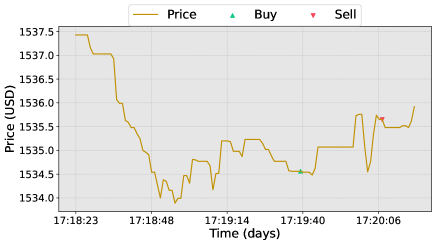
Figure 2: Trading process of EarnHFT in ETH

6.2 The Effectiveness of Hierarchical Framework

We examine the effectiveness of the hierarchical framework by analyzing the router’s behaviors under different datasets and conducting experiments to show the performance comparison of the EarHFT and each agent from its pool. From Figure 3 we can see that bull and rally agent tends to buy and hold and therefore perform well in the bull market (e.g., GALA). The sideways agent tends to trade less and hold still its position. The pullback and bear market tends to close its position and perform well in the bear market (e.g., ETH). The router combines all the advantages of the agents and performs the best on all 4 datasets in terms of profit. Figure 4 refers to the selection distribution for the router on 4 datasets. While datasets with high volatility (e.g., ETH and GALA), the market dynamics change more frequently and therefore the routing shows a more balanced distribution across 5 market trends. While datasets with lower volatility (e.g., BTCT and BTCU), the router selection is more focused on two market dynamics.

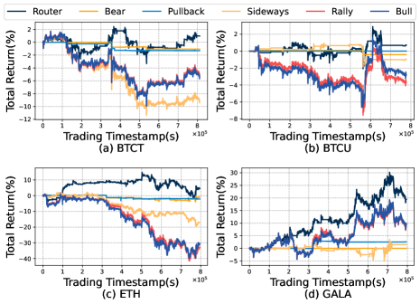
Figure 3: Comparison of the router and agent pool

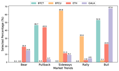
Figure 4: Router selection distribution

6.3 The Effectiveness of Optimal Action Value

OA	OS	GALA			ETH
		CS	RS	AHL	CS	RS	AHL
✓	✓	78848	4.43	448	102400	12.32	81.3
✓		102400	0.24	38.7	102400	-1.40	4.15
	✓	4608	2.89	147	30720	4.87	35.8
		30720	-0.01	284	30720	-29.6	39.1

Table 3: Ablation Study of OS and OT

To demonstrate the effectiveness of the optimal value supervisor (OS) and the optimal actor (OA), we conduct an ablation study on two datasets, ETH and GALA. We evaluate the training efficiency by the number of steps need to converge (CS) and the converged reward sum (RS). We further investigate their influence on agent trading behavior by average holding length (AHL). In Table 3. For GALA we can see that compared with the original DDQN, the one with OS only takes 15% of the steps to converge and gain a higher return. OA can further improve the return in exchange for more steps to converge. For ETH, since the market is bull, the CS is not reduced by OS. However, the return is largely increased. The reason why OS is more effective is that OS provides more information for the agents and its instructions vary along the changes of the agents’ policy while OA only provides demonstrations.

7 Conclusion

In this paper, we propose EarnHFT, a novel three-stage hierarchical RL framework for HFT to alleviate training efficiency and data shifting. First, we compute the optimal action value to improve the performance and training efficiency of second-level RL agents. Then we train a diverse pool of agents excelling in various market trends. Finally, we train a router to regularly pick an agent from the pool to conduct trading to deal with the dynamic market. Extensive experiments on Crypto markets demonstrate that EarnHFT significantly outperforms many strong baselines. Ablation studies show the effectiveness of the proposed components.

References

- Almeida and Gonçalves (2023) Almeida, J.; and Gonçalves, T. C. 2023. A systematic literature review of investor behavior in the cryptocurrency markets. Journal of Behavioral and Experimental Finance, 37: 100785.
- Briola et al. (2021) Briola, A.; Turiel, J.; Marcaccioli, R.; and Aste, T. 2021. Deep reinforcement learning for active high frequency trading. arXiv preprint arXiv:2101.07107.
- Chordia, Roll, and Subrahmanyam (2002) Chordia, T.; Roll, R.; and Subrahmanyam, A. 2002. Order imbalance, liquidity, and market returns. Journal of Financial Economics, 65(1): 111–130.
- Cumming, Alrajeh, and Dickens (2015) Cumming, J.; Alrajeh, D. D.; and Dickens, L. 2015. An investigation into the use of reinforcement learning techniques within the algorithmic trading domain. Imperial College London: London, UK, 58.
- Delfabbro, King, and Williams (2021) Delfabbro, P.; King, D. L.; and Williams, J. 2021. The psychology of cryptocurrency trading: Risk and protective factors. Journal of Behavioral Addictions, 10(2): 201–207.
- Hochreiter and Schmidhuber (1997) Hochreiter, S.; and Schmidhuber, J. 1997. Long short-term memory. Neural computation, 9(8): 1735–1780.
- Huang, Huang, and Ni (2019) Huang, J.-Z.; Huang, W.; and Ni, J. 2019. Predicting bitcoin returns using high-dimensional technical indicators. The Journal of Finance and Data Science, 5(3): 140–155.
- Huang et al. (2022) Huang, S.; Dossa, R. F. J.; Ye, C.; Braga, J.; Chakraborty, D.; Mehta, K.; and Araújo, J. G. 2022. Cleanrl: High-quality single-file implementations of deep reinforcement learning algorithms. The Journal of Machine Learning Research, 23(1): 12585–12602.
- Krug, Dobaj, and Macher (2022) Krug, T.; Dobaj, J.; and Macher, G. 2022. Enforcing network safety-margins in industrial process control using MACD indicators. In European Conference on Software Process Improvement, 401–413.
- Madhavan (2000) Madhavan, A. 2000. Market microstructure: A survey. Journal of Financial Markets, 3(3): 205–258.
- Mnih et al. (2013) Mnih, V.; Kavukcuoglu, K.; Silver, D.; Graves, A.; Antonoglou, I.; Wierstra, D.; and Riedmiller, M. 2013. Playing Atari with deep reinforcement learning. arXiv preprint arXiv:1312.5602.
- Mnih et al. (2015) Mnih, V.; Kavukcuoglu, K.; Silver, D.; Rusu, A. A.; Veness, J.; Bellemare, M. G.; Graves, A.; Riedmiller, M.; Fidjeland, A. K.; Ostrovski, G.; et al. 2015. Human-level control through deep reinforcement learning. Nature, 518(7540): 529–533.
- Muda, Begam, and Elamvazuthi (2010) Muda, L.; Begam, M.; and Elamvazuthi, I. 2010. Voice recognition algorithms using mel frequency cepstral coefficient (MFCC) and dynamic time warping (DTW) techniques. arXiv preprint arXiv:1003.4083.
- Niu, Li, and Li (2022) Niu, H.; Li, S.; and Li, J. 2022. MetaTrader: An reinforcement learning approach integrating diverse policies for portfolio optimization. In Proceedings of the 31st ACM International Conference on Information & Knowledge Management, 1573–1583.
- Purkayastha, Manolova, and Edelman (2012) Purkayastha, S.; Manolova, T. S.; and Edelman, L. F. 2012. Diversification and performance in developed and emerging market contexts: A review of the literature. International Journal of Management Reviews, 14(1): 18–38.
- Schulman et al. (2017) Schulman, J.; Wolski, F.; Dhariwal, P.; Radford, A.; and Klimov, O. 2017. Proximal policy optimization algorithms. arXiv preprint arXiv:1707.06347.
- Shiryaev (2008) Shiryaev, X. Y. 2008. Thou shalt buy and hold. Quantitative Finance, 8(8): 765–776.
- Silverman (1984) Silverman, B. W. 1984. Spline smoothing: the equivalent variable kernel method. The Annals of Statistics, 898–916.
- Sun et al. (2023) Sun, S.; Wang, X.; Xue, W.; Lou, X.; and An, B. 2023. Mastering stock markets with efficient mixture of diversified trading experts. Proceedings of the 29th ACM SIGKDD International Conference on Knowledge Discovery & Data Mining.
- Sun et al. (2022) Sun, S.; Xue, W.; Wang, R.; He, X.; Zhu, J.; Li, J.; and An, B. 2022. DeepScalper: A Risk-aware reinforcement learning framework to capture fleeting intraday trading opportunities. In Proceedings of the 31st ACM International Conference on Information & Knowledge Management, 1858–1867.
- Sutton and Barto (2018) Sutton, R. S.; and Barto, A. G. 2018. Reinforcement learning: An introduction. MIT press.
- Théate and Ernst (2021) Théate, T.; and Ernst, D. 2021. An application of deep reinforcement learning to algorithmic trading. Expert Systems with Applications, 173: 114632.
- Van Hasselt, Guez, and Silver (2016) Van Hasselt, H.; Guez, A.; and Silver, D. 2016. Deep reinforcement learning with double q-learning. In Proceedings of the AAAI Conference on Artificial Intelligence.
- Wang et al. (2021) Wang, R.; Wei, H.; An, B.; Feng, Z.; and Yao, J. 2021. Commission fee is not enough: A hierarchical reinforced framework for portfolio management. In Proceedings of the AAAI Conference on Artificial Intelligence, volume 35, 626–633.
- Zhang et al. (2023a) Zhang, C.; Duan, Y.; Chen, X.; Chen, J.; Li, J.; and Zhao, L. 2023a. Towards Generalizable Reinforcement Learning for Trade Execution. arXiv preprint arXiv:2307.11685.
- Zhang et al. (2023b) Zhang, C.; Duan, Y.; Chen, X.; Chen, J.; Li, J.; and Zhao, L. 2023b. Towards generalizable reinforcement learning for trade execution. arXiv:2307.11685.
- Zhou et al. (2021) Zhou, L.; Qin, K.; Torres, C. F.; Le, D. V.; and Gervais, A. 2021. High-frequency trading on decentralized on-chain exchanges. In 2021 IEEE Symposium on Security and Privacy (SP), 428–445.
- Zhu and Zhu (2022) Zhu, T.; and Zhu, W. 2022. Quantitative trading through random perturbation Q-network with nonlinear transaction costs. Stats, 5(2): 546–560.