The impact of angle-dependent partial frequency redistribution
on the scattering polarization of the solar Na i D lines

Abstract

The long-standing paradox of the linear polarization signal of the Na i D₁ line was recently resolved by accounting for the atom’s hyperfine structure and the detailed spectral structure of the incident radiation field. That modeling relied on the simplifying angle-averaged (AA) approximation for partial frequency redistribution (PRD) in scattering, which potentially neglects important angle-frequency couplings. This work aims at evaluating the suitability of a PRD–AA modeling for the D₁ and D₂ lines through comparisons with general angle-dependent (AD) PRD calculations, both in the absence and presence of magnetic fields. We solved the radiative transfer problem for polarized radiation in a one-dimensional semi-empirical atmospheric model with microturbulent and isotropic magnetic fields, accounting for PRD effects, comparing PRD–AA and PRD–AD modelings. The D₁ and D₂ lines are modeled separately as two-level atomic system with hyperfine structure. The numerical results confirm that a spectrally structured radiation field induces linear polarization in the D₁ line. However, the PRD–AA approximation greatly impacts the $Q/I$ shape, producing an antisymmetric pattern instead of the more symmetric PRD–AD one, while presenting a similar sensitivity to magnetic fields between $10$ and $200$ G. Under the PRD–AA approximation, the $Q/I$ profile of the D₂ line presents an artificial dip in its core, which is not found for the PRD–AD case. We conclude that accounting for PRD–AD effects is essential to suitably model the scattering polarization of the Na i D lines. These results bring us closer to exploiting the full diagnostic potential of these lines for the elusive chromospheric magnetic fields.

1 Introduction

Measurements of the polarization of the solar radiation are an essential resource for exploring the properties of the solar atmosphere, and especially its magnetism. High-precision spectro-polarimetric observations performed in quiet regions of the Sun close to the limb reveal numerous and varied linear polarization features that are collectively referred to as the Second Solar Spectrum (e.g., Stenflo & Keller, 1997; Gandorfer, 2002). These polarization signals are produced by the scattering of anisotropic radiation (i.e., scattering polarization). During the scattering process, the radiation induces population imbalances and coherence between atomic states that belong to the same level or term (i.e., atomic level polarization). The presence of a magnetic field modifies the atomic level polarization, and thus scattering polarization, via the Hanle effect. Each spectral line is sensitive to the Hanle effect in a given range of field strengths, depending on the Landé factors and the lifetimes of the levels involved in the spectral line transition (e.g., Trujillo Bueno, 2001). Nowadays, the power of magnetic field diagnostics based on the joint action of the Hanle and Zeeman effects is well established, especially for obtaining information on photospheric, chromospheric, and coronal magnetic fields outside active regions (e.g., Trujillo Bueno & del Pino Alemán, 2022, and references therein).

A particularly interesting instance of scattering polarization, and the focus of this work, was observed by Stenflo & Keller (1997). The conspicuous linear polarization signal they reported in the core region of Na i D₁ at 5896 Å eluded a straightforward explanation because this line, which arises from an atomic transition between an upper and lower level that both have total angular momentum $J=1/2$, was considered to be intrinsically unpolarizable. Subsequent investigations that aimed at providing a theoretical explanation for these enigmatic signals relied on the fact that sodium has nuclear spin $I=3/2$ and, hence, its fine-structure (FS) levels split into several hyperfine-structure (HFS) levels. Accounting for HFS, and assuming that the lower level of D₁ (the ground level of sodium) has a substantial amount of atomic polarization, Landi Degl’Innocenti (1998) could successfully fit the observed D₁ polarization signals. However, the required amount of ground level atomic polarization was incompatible with the presence of inclined magnetic fields stronger than about $0.01$ G, whereas theoretical plasma physics arguments and observations in other spectral lines suggest that far stronger fields should be ubiquitous in the quiet solar chromosphere. Finding a resolution to this paradox represented a serious challenge to solar physicists for many years.

Several years later, a breakthrough in the modeling of the Na i D₁ line was presented by Belluzzi & Trujillo Bueno (2013). For the unmagnetized case, these authors showed that scattering polarization signals of substantial amplitude could be produced without the need for ground-level polarization (see also Belluzzi et al., 2015). It was demonstrated that such linear polarization signals can be explained by taking into account the detailed spectral structure of the incident anisotropic radiation over the small wavelength intervals spanned by the HFS transitions that compose the D₁ line, so that the various HFS components can possibly be pumped by a slightly different radiation field. It must be stressed that within the framework of a first-order theory of polarization, that is considering the limit of complete frequency redistribution (CRD), it is not possible to account for this differential pumping together with the impact of coherence between different HFS levels, because this would not comply with the flat-spectrum condition (see Landi Degl’Innocenti & Landolfi, 2004). To accurately model these effects, it is therefore necessary to formulate the problem using high-order approaches, which include partial frequency redistribution (PRD) effects (i.e., frequency correlations between incident and scattered radiation). The suitability of this explanation was confirmed when Alsina Ballester et al. (2021) modeled the polarization of the solar sodium doublet radiation accounting for both collisions and magnetic fields, within the framework of the quantum theory of spectral line polarization described in Bommier (2017). They also highlighted the sensitivity of these polarization signals to the presence of magnetic fields in the gauss range, opening up a new window for probing the elusive magnetic fields of the solar chromosphere in the present new era of large-aperture solar telescopes.

Because of the high computational requirements of modeling these scattering polarization signals, Alsina Ballester et al. (2021) made the so-called angle-averaged (AA) simplifying assumption in their calculations (see, e.g., Rees & Saliba 1982; Sampoorna 2014 and references therein; Belluzzi & Trujillo Bueno 2014; Alsina Ballester et al. 2017), which accounted for the HFS of sodium and for the quantum interference between states belonging to different FS levels of the upper term (i.e., $J$-state interference) and between states belonging to different HFS levels of the same HFS level (i.e., $F$-state interference). As summarized in Section 2.1, the AA approximation smears out geometrical dependencies of the problem, and can, in principle, introduce significant inaccuracies in the synthesized profiles (see, e.g., Janett et al., 2021a).

The aim of this work is to evaluate the suitability of angle-averaging in this context through a comparison with angle-dependent (AD) PRD calculations, which are more accurate but have a significantly higher numerical cost. For this goal, we carried out a series of calculations with a code capable of solving the non-local-thermodynamical-equilibrium (non-LTE) RT problem in static 1D semi-empirical models of the solar atmosphere for two-level model atoms (in which $J$-state interference are neglected) with HFS, taking scattering polarization and PRD–AD effects into account.

The article is organized as follows: Section 2 exposes the considered RT problem for polarized radiation and outlines the adopted solution strategy. Section 3 describes the considered atomic and atmospheric models. In Section 4, we report and analyze the synthetic emergent Stokes profiles of the Na i D₁ and D₂ lines, comparing PRD–AA and PRD–AD calculations. Finally, Section 5 provides remarks and conclusions.

2 Transfer problem for polarized radiation

The intensity and polarization of a radiation beam are fully described by the four Stokes parameters $I$, $Q$, $U$, and $V$. The Stokes parameter $I$ quantifies the intensity, $Q$ and $U$ jointly quantify the linear polarization, while $V$ quantifies the circular polarization (e.g., Landi Degl’Innocenti & Landolfi, 2004). Hereafter, we will assume stationary conditions so that all the considered quantities are time-independent.

The intensity and polarization of a radiation beam propagating in a medium (e.g., the plasma of a stellar atmosphere) change as the radiation interacts with the particles therein. This modification is fully described by the RT equation for polarized radiation, which is a system of coupled first-order, inhomogeneous, ordinary differential equations. Defining the Stokes parameters as the four components of the Stokes vector $\bm{I}=(I_{1},I_{2},I_{3},I_{4})^{T}=(I,Q,U,V)^{T}\in\mathbb{R}^{4}$, the RT equation can be written as

$$\vec{\nabla}_{{\bm{\Omega}}}\bm{I}(\bm{r},\bm{\Omega},\nu)=-K(\bm{r},\bm{\Omega},\nu)\,\bm{I}(\bm{r},\bm{\Omega},\nu)+\bm{\varepsilon}(\bm{r},\bm{\Omega},\nu),$$ (1)

where $\bm{r}$ denotes the spatial point, $\nu$ the radiation frequency, and $\vec{\nabla}_{\bm{\Omega}}$ denotes the spatial derivative along the direction specified by the unit vector $\bm{\Omega}=(\theta,\chi)$, $\theta$ and $\chi$ being the polar angles (inclination and azimuth, respectively). The propagation matrix $K\in\mathbb{R}^{4\times 4}$ is given by

$$K=\begin{pmatrix}\eta_{1}&\eta_{2}&\eta_{3}&\eta_{4}\\ \eta_{2}&\eta_{1}&\rho_{4}&-\rho_{3}\\ \eta_{3}&-\rho_{4}&\eta_{1}&\rho_{2}\\ \eta_{4}&\rho_{3}&-\rho_{2}&\eta_{1}\\ \end{pmatrix}.$$ (2)

The elements of $K$ describe absorption ($\eta_{1}$), dichroism ($\eta_{2}$, $\eta_{3}$, and $\eta_{4}$), and anomalous dispersion ($\rho_{2}$, $\rho_{3}$, and $\rho_{4}$) phenomena. The emission vector $\bm{\varepsilon}=(\varepsilon_{1},\varepsilon_{2},\varepsilon_{3},\varepsilon_{4})^{T}\in\mathbb{R}^{4}$ describes the radiation emitted by the plasma in the four Stokes parameters.

In the frequency interval of a given spectral line, the elements of $K$ and $\bm{\varepsilon}$ depend on the state of the atom (or molecule) giving rise to that line. In general, this state has to be determined by solving a set of rate equations (statistical equilibrium equations), which describe the interaction of the atom with the radiation field (radiative processes), other particles present in the plasma (collisional processes), and external magnetic and electric fields. The emission vector, in particular, can be written as the sum of two terms, namely

$$\bm{\varepsilon}(\bm{r},\bm{\Omega},\nu)=\bm{\varepsilon}^{\mathrm{sc}}(\bm{r},\bm{\Omega},\nu)+\bm{\varepsilon}^{\mathrm{th}}(\bm{r},\bm{\Omega},\nu),$$ (3)

where $\bm{\varepsilon}^{\mathrm{sc}}$ describes the contribution from atoms that are radiatively excited (scattering term), and $\bm{\varepsilon}^{\mathrm{th}}$ describes the contribution due to atoms that are collisionally excited (thermal term). We note that, in the solar atmosphere, stimulated emission is negligible in the spectral interval around the Na i D lines and it is consequently neglected. For certain, relatively simple, atomic models (for instance a two-term atomic system with an unpolarized lower term whose levels are infinitely sharp), an analytic solution exists for the statistical equilibrium equations. In such scenarios, the scattering contribution to the emission vector can be directly related to the radiation field that illuminates the atom (incident radiation) through the redistribution matrix formalism. Following the convention that primed and unprimed quantities refer to the incident and scattered radiation, respectively, it can be written in terms of the so-called scattering integral

$$\small\bm{\varepsilon}^{\mathrm{sc}}(\bm{r},\bm{\Omega},\nu)=k_{L}(\bm{r})\!\!\int\!\!\mathrm{d}\nu^{\prime}\!\!\oint\frac{\mathrm{d}\bm{\Omega}^{\prime}}{4\pi}R(\bm{r},\bm{\Omega}^{\prime},\bm{\Omega},\nu^{\prime},\nu)\,\bm{I}(\bm{r},\bm{\Omega}^{\prime},\nu^{\prime}),$$ (4)

where the factor $k_{L}$ is the frequency-integrated absorption coefficient, and $R\in\mathbb{R}^{4\times 4}$ is the redistribution matrix. The element $R_{ij}(\bm{r},\bm{\Omega}^{\prime},\bm{\Omega},\nu^{\prime},\nu)$ of the redistribution matrix relates the $i$-th Stokes component of the emissivity, in direction $\bm{\Omega}$ and at frequency $\nu$, to the $j$-th Stokes component of the incident radiation with direction $\bm{\Omega}^{\prime}$ and frequency $\nu^{\prime}$.

For an atomic system with infinitely sharp lower states, as the one considered in this work (see Section 3 for more details), the redistribution matrix can be separated into

$$R(\bm{r},\bm{\Omega}^{\prime},\bm{\Omega},\nu^{\prime},\nu)=R^{\scriptscriptstyle\mathrm{II}}(\bm{r},\bm{\Omega}^{\prime},\bm{\Omega},\nu^{\prime},\nu)+R^{\scriptscriptstyle\mathrm{III}}(\bm{r},\bm{\Omega}^{\prime},\bm{\Omega},\nu^{\prime},\nu),$$

where the notation introduced in Hummer (1962) has been used. The $R^{\scriptscriptstyle\mathrm{II}}$ matrix quantifies scattering processes that are coherent in the rest frame of the atom and $R^{\scriptscriptstyle\mathrm{III}}$ quantifies those that are totally incoherent due to the impact of elastic collisions. The expressions for $R^{\scriptscriptstyle\mathrm{II}}$ and $R^{\scriptscriptstyle\mathrm{III}}$ in the observer’s frame (i.e., including the Doppler shifts due to thermal atomic motions) in the case of a two-term atom can be obtained from Equation (A.1) of Bommier (2018). The same redistribution matrices, particularized to the case of a Maxwellian distribution of atomic velocities (without a bulk component) under the AA approximation (see Section 2.1), as well as the $K$ matrix elements, can be found in Alsina Ballester et al. (2022). The thermal contribution to the emissivity $\bm{\varepsilon}^{\mathrm{th}}$ can be found, for instance, in Alsina Ballester (2022). In this work, we also include the contribution brought by continuum processes. In the considered spectral region, they only contribute to the diagonal elements of $K$. The continuum emissivity is calculated including both the thermal contribution (assumed to be isotropic and unpolarized) and the scattering one (under the assumption of coherent scattering in the observer’s frame). More details on the continuum terms can be found in Sect. 2.5 of Alsina Ballester et al. (2022).

Solving the whole RT problem consists in finding a self-consistent solution for the RT equation (1) and the equation for the scattering contribution to the emissivity (4). This problem is in general non-linear because of the factor $k_{L}$ that appears both in the elements of the propagation matrix and in the emission coefficients. This factor is proportional to the population of the lower level, which in turn depends non-linearly on the incident radiation field through the statistical equilibrium equations.

We linearize the problem with respect to $\bm{I}$, by fixing a priori the population of the lower level, and thus the factor $k_{L}$. In this scenario, whose suitability is discussed in Janett et al. (2021b) and Benedusi et al. (2021), the propagation matrix $K$ and the thermal contribution to the emissivity $\bm{\varepsilon}^{\mathrm{th}}$ are independent of $\bm{I}$, while the scattering term $\bm{\varepsilon}^{\mathrm{sc}}$ depends on it linearly through the scattering integral shown in Equation (4). The population of the lower level can be taken either from the atmospheric model (if provided) or from independent calculations. The latter can be carried out with available non-LTE RT codes that neglect polarization (which is expected to have a minor impact on the population of ground or metastable levels), but allow considering multi-level atomic models. In this way, accurate estimates of the lower level population can be used (e.g., Janett et al., 2021a; Alsina Ballester et al., 2021).

2.1 Angle-averaged approximation

Using the formalism of the irreducible spherical tensors for polarimetry (e.g., Chapt. 5 of Landi Degl’Innocenti & Landolfi, 2004), the ${R}^{{\scriptscriptstyle\rm II}}$ and ${R}^{{\scriptscriptstyle\rm III}}$ redistribution matrices can be decomposed as

$$R^{\scriptscriptstyle X}\!(\bm{r},\bm{\Omega}^{\prime}\!,\bm{\Omega},\nu^{\prime}\!,\nu)\!=\!\!\!\sum_{KK^{\prime}Q}\!\!\!\mathcal{R}^{{\scriptscriptstyle X},KK^{\prime}}_{Q}\!(\bm{r},\bm{\Omega}^{\prime},\bm{\Omega},\nu^{\prime}\!,\nu)P^{KK^{\prime}}_{Q}\!(\bm{r},\bm{\Omega}^{\prime},\bm{\Omega}),$$

with $X=\{\mathrm{II},\mathrm{III}\}$. The scattering phase matrix $P$ is independent of frequency and its expression can be found, e.g., in Alsina Ballester et al. (2022). The $\mathcal{R}^{{\scriptscriptstyle X}}$ redistribution function locally couples all frequencies and directions of the incident and scattered radiation, making the problem computationally very demanding. In the absence of bulk velocities, the angular dependence of this function is fully contained in the scattering angle

$$\Theta=\arccos\left(\bm{\Omega}^{\prime}\cdot\bm{\Omega}\right).$$

Approximated forms of the functions $\mathcal{R}^{{\scriptscriptstyle X}}$ are frequently applied to simplify the calculations. A common one for $\mathcal{R}^{{\scriptscriptstyle\rm II}}$ is the so-called AA, which consists in averaging this function over the scattering angle $\Theta$, namely

$$\mathcal{R}^{{\scriptscriptstyle\rm II-AA},KK^{\prime}}_{Q}\!(\bm{r},\nu^{\prime},\nu)=\frac{1}{2}\!\int_{0}^{\pi}\!\!\!{\rm d}{\Theta}\sin(\Theta)\,\mathcal{R}^{{\scriptscriptstyle\rm II},KK^{\prime}}_{Q}\!(\bm{r},\bm{\Omega}^{\prime},\bm{\Omega},\nu^{\prime},\nu).$$ (5)

When the AA redistribution function (5) is used, frequencies and directions are completely decoupled in $\mathcal{R}^{{\scriptscriptstyle\rm II}}$, allowing for a drastic reduction of the computational cost.

Faurobert (1987, 1988) and Sampoorna et al. (2011, 2017) analyzed the suitability of the AA approximation in the modeling of polarization signals in academic scenarios, concluding that this approximation introduces relevant inaccuracies in the modeling of the linear polarization signals in the core of spectral lines. More recently, Janett et al. (2021a) showed that the AA approximation introduces an artificial trough in the line-core peak of the $Q/I$ and $U/I$ scattering polarization profiles of the Ca i 4227 line. This highlights the need to evaluate the impact of this approximation when modeling the scattering polarization of lines where PRD effects play a crucial role, like for the D lines of neutral sodium.

Leenaarts et al. (2012) proposed a generalization of the AA approximation suited for dynamic scenarios, which proved to be highly effective for the unpolarized case. This version of the AA approximation sacrifices information on the anisotropy of the radiation field, and it is thus not suited for the description of scattering polarization. However, the AA approximation for the polarized case can be also used in dynamic scenarios by applying the comoving frame method for treating bulk velocities (see Sampoorna & Nagendra, 2016, and references therein). We note that the radiative transfer equation in the comoving frame includes an additional term containing a derivative w.r.t. frequency, yielding a partial differential equation, which is significantly more complicated to solve (see, e.g., Mihalas, 1978, p. 492).

As far as $\mathcal{R}^{{\scriptscriptstyle\rm III}}$ is concerned, a widely used approximation is to assume that the scattering processes described by this matrix are totally incoherent also in the observer’s frame (e.g., Mihalas, 1978; Bommier, 1997; Alsina Ballester et al., 2017; Benedusi et al., 2022). This assumption is also applied in this work.

2.2 Numerical solution strategy

Following the works by Janett et al. (2021b) and Benedusi et al. (2021, 2022), we first present an algebraic formulation of the considered linearized RT problem for polarized radiation. Starting from this formulation, we then apply a parallel solution strategy, based on Krylov iterative methods with physics-based preconditioning. This strategy allows us to routinely solve the problem in semi-empirical 1D models of the solar atmosphere, considering the angle-dependent expression of $R^{\scriptscriptstyle\rm II}$.

The problem is discretized by introducing suitable grids for the continuous variables $\bm{r}$, $\theta$, $\chi$, and $\nu$ (see Section 4.1). Provided the radiation field at all nodes on the angular grid $(\theta_{l},\chi_{m})$ ($l=1,...,N_{\theta}$, $m=1,...,N_{\chi}$) and frequency grid $\nu_{j}$ ($j=1,...,N_{\nu}$), for a given spatial grid point $\bm{r}_{i}$ ($i=1,....,N_{r}$), the scattering integral (4) is evaluated in terms of suitable angular and spectral quadratures. Provided the propagation matrix (2) and the emission coefficients (3) at all spatial points $\bm{r}_{i}$, for a given direction $(\theta_{l},\chi_{m})$ and frequency $\nu_{j}$, the RT equation (1) is numerically solved by applying the $L$-stable DELO-linear method combined with a linear conversion to optical depth (see, e.g., Janett et al., 2017; Janett & Paganini, 2018; Janett et al., 2018). In Equation (1) we impose the following boundary conditions: we assume that no radiation is entering from the upper boundary, while the radiation entering the atmosphere from the lower boundary is assumed isotropic, unpolarized, and equal to the Planck function.

After introducing the collocation vectors $\mathbf{I}\in\mathbb{R}^{N}$ and $\bm{\epsilon}\in\mathbb{R}^{N}$ $(N=4N_{r}\,N_{\nu}\,N_{\theta}\,N_{\chi})$, which contain the numerical approximations of the Stokes vector and the emission vector, respectively, at all $N$ nodes, the whole discrete RT problem can be then formulated in the compact form given by (see Janett et al., 2021a; Benedusi et al., 2022)

$$(Id-\Lambda\Sigma)\mathbf{I}=\Lambda\bm{\epsilon}^{\mathrm{th}}+\mathbf{t}.$$ (6)

In this linear system, $Id\in\mathbb{R}^{N\times N}$ is the identity matrix. $\Lambda:\mathbb{R}^{N}\rightarrow\mathbb{R}^{N}$ is the transfer operator, which encodes the formal solver and the propagation matrix. The scattering operator, which encodes the numerical evaluation of the scattering integral (4), is given by the sum of different components, namely,

$$\Sigma=\Sigma^{\scriptscriptstyle\rm II}+\Sigma^{\scriptscriptstyle\rm III}+\Sigma^{\rm c},$$

where $\Sigma^{\scriptscriptstyle\rm II}$ and $\Sigma^{\scriptscriptstyle\rm III}$ encode the contributions from $R^{\scriptscriptstyle\rm II}$ and $R^{\scriptscriptstyle\rm III}$, respectively, and $\Sigma^{\rm c}$ the scattering contribution from the continuum. The vector $\bm{\epsilon}^{\rm th}\in\mathbb{R}^{N}$ encodes the thermal emissivity, and the vector $\mathbf{t}\in\mathbb{R}^{N}$ encodes the boundary conditions.

Under the assumption that $k_{L}$ is known a priori (see, e.g., Janett et al., 2021a), the operators $\Lambda$ and $\Sigma$ do not depend on $\mathbf{I}$, and the problem (6) is thus linear. The right-hand side vector $\Lambda\bm{\epsilon}^{\mathrm{th}}+\mathbf{t}$ is computed a priori, while the action of the matrices $\Lambda$ and $\Sigma$ is encoded in a matrix-free form. We solve the linear system (6) by applying a matrix-free, preconditioned GMRES method. Figure 1 illustrates the convergence history for preconditioned and unpreconditioned GMRES iterative methods applied to (6), by modeling the Na i D₁ line via the numerical setting described in Section  4.1, in the absence of magnetic fields. In particular, we exploit two different preconditioners based on two simplified descriptions of the scattering process: (i) by considering the limit of CRD and (ii) by applying the AA approximation. Both CRD- and PRD–AA-based preconditioners have a noticeable impact. We note that the computational cost for the former is substantially lower than for the latter. In the calculations presented in this paper, preconditioning is thus performed by describing scattering processes in the limit of CRD. The preconditioned GMRES solvers outperform the unpreconditioned one, strongly reducing the number of iterations to convergence. The reader is referred to Benedusi et al. (2022) for more details on this solution strategy.

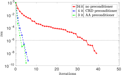
Figure 1: Convergence history for the GMRES iterative solution of (6) for the Na i D₁ line, exploiting none, CRD, and PRD–AA preconditioners. The number of iterations to convergence are reported in square brackets. The horizontal dashed line represents the tolerance (${\rm tol}=10^{-6}$) for the preconditioned relative residual (${\rm res}$).

3 Atomic and atmospheric models

In this section, we present the atomic and the atmospheric models used in the calculations. A strictly correct RT modeling of the scattering polarization of the Na i D lines should be carried out considering a two-term atom with HFS (see Alsina Ballester et al., 2021). The upper term (${}^{2}\mathrm{P}^{o}$) consists of two FS $J$ levels, having total angular momentum $J=1/2$ (upper level of D₁) and $J=3/2$ (upper level of D₂). The lower term (${}^{2}\mathrm{S}$) consists of the ground level of sodium with $J=1/2$, which is the lower level of both D₁ and D₂. Because this level has a very long lifetime, all its sublevels can be taken to be infinitely sharp. The lower level can also be treated as unpolarized; because of its long lifetime, it is strongly depolarized by magnetic fields of just a few tens of milligauss (Landi Degl’Innocenti, 1998) and by elastic collisions with neutral hydrogen, for densities as low as $n_{\mathrm{H}}\sim 10^{14}$cm³ (see Kerkeni & Bommier, 2002). Due to the interaction with the nuclear spin ($I=3/2$), the $J$ levels split into various HFS $F$ levels.

In the presence of external magnetic fields such that the splitting between magnetic sublevels is comparable to the separation between HFS or FS levels, their energies must be calculated in the incomplete Paschen-Back (IPB) effect regime, accounting for the related mixing between eigenstates of total angular momentum.

Because of the large energy separation between the upper $J$ levels of D₁ and D₂, the $J$-state interference between them is not appreciably modified by the presence of a magnetic field, and it only affects the scattering polarization pattern outside the line core regions. This can be seen from the similarities between the synthetic $Q/I$ profiles shown in Figure 4 of Belluzzi & Trujillo Bueno (2013) and in Figure 1 of Belluzzi et al. (2015), in which $J$-state interference was taken into account and neglected, respectively. We also verified this using the more recent numerical code described in Alsina Ballester et al. (2022), which is suitable for modeling lines that arise from a two-term atomic system with HFS, in the presence of arbitrary magnetic fields, under the AA approximation.

3.1 Two-level atom with HFS for Na i D lines

At the time of writing, no numerical code exists that can handle the computational complexity of the non-LTE RT problem for polarized radiation for a two-term atom with HFS, while accounting for PRD effects in the general AD case. However, bearing in mind that $J$-state interference does not significantly modify the line-core polarization signals of the Na i D lines, for the purposes of this work we find it suitable to model the D1 and D2 lines separately, considering a two-level atom with HFS for each of them. A similar strategy was followed by Sampoorna et al. (2019) and Nagendra et al. (2020) in their PRD-AA vs PRD-AD investigation of the Na i D₂ line in isothermal slab models. The D₁ (D₂) line is modeled setting $J_{\ell}=1/2$ and $J_{u}=1/2\,\,(3/2)$, and taking into account the HFS due to a nuclear spin $I=3/2$. The calculations are carried out using existing codes for a two-term atom without HFS, and applying them to the formally equivalent case of a two-level atom with HFS (e.g., Landi Degl’Innocenti & Landolfi, 2004). In the unmagnetized case, the equivalence between a two-term atom and a two-level atom with HFS is obtained with the following formal substitutions in the quantum numbers: $S\rightarrow I$, $L\rightarrow J$, $J\rightarrow F$ (see also Eq. (A6)), where $S$ and $L$ have the usual meaning of total electronic spin and orbital angular momentum quantum numbers, respectively. The generalization to the magnetic case is described in Appendix A. We used experimental data for the energies of the upper $J$ levels (Kramida et al., 2022). The energy splittings of the HFS $F$ levels were calculated using recent experimental values for the HFS constants for the various $J$ levels (Steck, 2003).

3.2 1D semi-empirical atmospheric model

In this work, we consider the 1D semi-empirical solar atmospheric model C of Fontenla et al. (1993) either in the absence or in the presence of microturbulent magnetic fields (see Section 3.3), taking the micro-turbulent velocities as determined semi-empirically in Fontenla et al. (1991). In a 1D model, the spatial dependency of the physical quantities entering the RT problem is fully described by the height coordinate $z$, which replaces the coordinate $\bm{r}$. In this work we do not consider deterministic magnetic fields and bulk velocities. The problem is thus characterized by axial symmetry, which allow us to keep computational costs down to a manageable level. It can be expected that the impact of the general AD treatment of PRD effects will be greater when the radiation field scattered by the atom has a more complex angular dependence, as happens when the complex 3D geometrical structure of the solar chromospheric plasma is taken into account (e.g., Benedusi et al., 2023; Anusha, 2023, and references therein).

3.3 Microstructured magnetic fields

In the solar atmosphere, it is common to find magnetic fields that vary on spatial scales below the resolution element of standard observations, which are often referred to as tangled (e.g. Trujillo Bueno et al., 2004; Manso Sainz et al., 2004). Throughout this work, we consider unimodal microstructured isotropic magnetic fields (see Stenflo, 1994; Trujillo Bueno & Manso Sainz, 1999; Alsina Ballester et al., 2017), that is, fields with a fixed strength but whose orientation changes at scales below the mean free path of photons, such that they are uniformly distributed over all directions. The expressions for the RT coefficients (i.e., elements of the propagation matrix and components of the emission vector) in the presence of such tangled magnetic fields are discussed in Alsina Ballester et al. (2022).

4 Numerical results

In this section, we provide quantitative results on the suitability of a PRD–AA modeling for the Na i D lines, through comparisons with the general PRD–AD calculations, both in the absence and presence of magnetic fields. As discussed in Section 3, the D₁ and D₂ lines are modeled separately, considering for each of them a two-level system with HFS, in which the Paschen-Back effect is taken into account for the magnetic splitting. This section focuses on the modeling of the D₁ line at 5896 Å, whereas the modeling of the D₂ line at 5890 Å is reported in Appendix B.

4.1 Numerical setting

The wavelength interval $[\lambda_{\min},\lambda_{\max}]=[5894.4\text{\,\AA},5897.4\text{\,\AA}]$ is discretized with ${N_{\nu}=161}$ logarithmically distributed nodes. This frequency grid, chosen to suitably sample the spectral line under investigation, is denser in the line core and coarser in the wings. The spatial grid is provided by the considered 1D semi-empirical atmospheric model C of Fontenla et al. (1993), which discretizes the height interval $[z_{\min},z_{\max}]=[-100~{}\text{km},2219~{}\text{km}]$ with $N_{r}=70$ unevenly distributed spatial nodes. We adopted a very common tensor product angular grid with $N_{\chi}=12$ and $N_{\theta}=12$, for a total of $N_{\Omega}=144$ nodes, which guarantees the accurate calculation of the scattering polarization signals (see Appendix C for details).

The proposed iterative solver consists of two nested GMRES iterations (see Benedusi et al., 2022). We use no restart and the same threshold tolerance ${\rm tol}$ for both GMRES iterations. As a stopping criterion for the iterative method, we adopt the inequality

$${\rm res}<{\rm tol}=10^{-6},$$

in which the preconditioned relative residual ${\rm res}$ is a scalar that indicates the accuracy of the approximate solution. We adopt a zero initial guess.

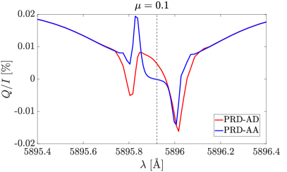
Figure 2: Emergent $Q/I$ profiles for the Na i D₁ line at $\mu=0.1$, calculated with a two-level model atom and in the atmospheric model C of Fontenla et al. (1993), without a magnetic field. The results of calculations are shown taking PRD effects into account both in the general AD case (red curve) and under the AA approximation (blue curve), in both cases neglecting the impact of $J$-state interference. The vertical dashed line indicates the line-center wavelength.

4.2 Impact of PRD–AD treatment on D₁ polarization

The intensity profiles of PRD–AA and PRD–AD calculations are essentially identical in all the considered cases, and thus they are not explicitly shown. Figure 2 shows the $Q/I$ patterns of the D₁ line obtained for PRD–AA and for PRD–AD calculations in the absence of magnetic fields, using the numerical scheme described in the previous sections. In order to have scattering polarization signals with a relatively large amplitude in the considered geometry, we show a significantly inclined line of sight with $\mu=\cos(\theta)=0.1$. The PRD–AA calculation yields a largely antisymmetric $Q/I$ profile around the D₁ line core, with a positive peak on the blue side of the line center, and a negative one on the red side. We find a very good qualitative agreement between this pattern and the one reported in Figure 4 of Belluzzi & Trujillo Bueno (2013), although a strict comparison cannot be made because different formal solvers were used. Likewise, it also presents a good qualitative agreement with the polarization signals in the D₁ core region shown in Figure 1 of Belluzzi et al. (2015) and in Figure 2 of Alsina Ballester et al. (2021). As expected, the $Q/I$ lobes outside the line core reported in the latter two investigations cannot be reproduced with the two-level atomic model considered in the present work, because such lobes arise from $J$-state interference.

The PRD–AD calculation yields a scattering polarization profile that presents substantial differences in the shape with respect to the PRD–AA calculation. Whereas a similar red negative peak is obtained for both treatments, the positive blue peak that was found in the PRD–AA case is shifted toward the line center for the PRD–AD calculation and a negative peak is found in its place. Thus, instead of the antisymmetric pattern resulting from the PRD–AA calculation, the PRD–AD calculation produces a far more symmetric profile, with a positive $Q/I$ peak near the line center and negative peaks at $\sim 0.1$ Å to the red and blue of it. We also note that the positive $Q/I$ peak found in the PRD–AD case does not fall exactly at line center, but instead its maximum is slightly shifted to the blue. When artificially neglecting the HFS splitting in the lower level, the resulting $Q/I$ profile only shows a depolarization feature in the line core. This confirms that the physical origin of the line scattering polarization is the same as for PRD–AA calculations, that is the variation of the anisotropy of the radiation field over the spectral range spanned by the HFS transitions of the D₁ line, as shown by Belluzzi & Trujillo Bueno (2013). Even though the linear polarization profile resulting from AD calculations is rather symmetric, in contrast to the mostly antisymmetric $Q/I$ profile obtained from AA calculations, it is noteworthy that the signal obtained from integrating the former over frequency is not greater than the one obtained when integrating the latter (see Appendix D).

Thus, a suitable modeling of the observed linear polarization patterns of the Na i D₁ line requires making a PRD–AD treatment of scattering processes, while considering a two-term atomic model (in order to account for the $J$-state interference) with HFS. We recall that an antisymmetric $Q/I$ profile of the Na i D₁, obtained from an observation with low temporal and spatial resolution, could be fit remarkably well considering PRD-AA calculations (see Alsina Ballester et al., 2021). We may expect that such antisymmetric profiles can be modeled also considering AD-PRD effects, once we additionally account for relevant phenomena such as the spectral smearing of typical instruments and local effects related to the three-dimensional and dynamic nature of the solar atmosphere. An investigation of these effects is, however, beyond the scope of both the aforementioned investigation and the present one. We also point out that new spectro-polarimetric observations have been recently acquired in the spectral range around the Na i D₁ line (e.g., Bianda et al., 2019). Such observations present a wide variety of profiles, a few of which are quite symmetric, with a shape in good qualitative agreement with the theoretical PRD–AD profiles presented above.

Figure 3 shows the same linear polarization profiles as in Figure 2, also comparing AD and AA calculations, but for various lines of sight (LOS). In the AA case (lower panel), the amplitude of the $Q/I$ peaks decreases for larger $\mu$, while its shape is largely preserved. In contrast, the shape of the AD profile (upper panel) clearly changes with the LOS; the overall $Q/I$ pattern becomes much more symmetric for larger $\mu$ values, as the shift of the central peak towards the blue becomes less pronounced. In addition, the amplitude of the three peaks does not decrease monotonically as $\mu$ increases, but instead they reach a maximum and then decrease. The central peak, for instance, reaches its maximum at around $\mu=0.61$.

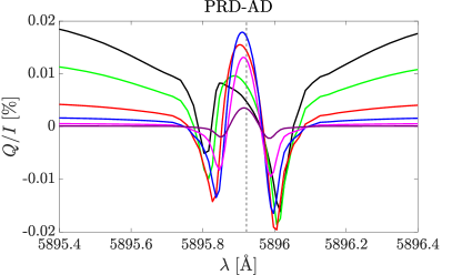
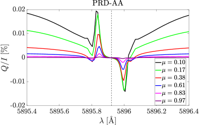
Figure 3: Emergent $Q/I$ profiles for the Na i D₁ line for different lines of sight, calculated in atmospheric model C of Fontenla et al. (1993), without a magnetic field. The results of calculations are shown taking PRD effects into account both in the general AD case (upper panel) and under the AA approximation (lower panel), in both cases neglecting the impact of $J$-state interference. The vertical dashed line indicates the line-center wavelength.

4.3 Impact of the magnetic fields on D₁ polarization

It is also of interest to investigate the sensitivity of the D₁ scattering polarization to magnetic fields. We recall that, in the presence of an isotropic distribution of micro-structured magnetic fields, such as the one considered in this work, the Zeeman and magneto-optical signatures vanish due to cancellation effects, and the only impact of the magnetic field is the modification of $Q/I$ due to the Hanle effect (see Alsina Ballester et al., 2021). The $U/I$ and $V/I$ signals are thus zero and are consequently not shown. The upper panel of Figure 4 shows the $Q/I$ patterns obtained from AD calculations in which we accounted for isotropic microturbulent magnetic fields of various strengths, in a range between $0$ and $100$ G, for which the incomplete Paschen-Back effect regime is attained. For field strengths of $20$ G, the amplitude of the D₁ $Q/I$ signal already decreases appreciably due to the Hanle effect, both in the positive peak near the line center and in the negative lateral peaks. At roughly $200$ G, Hanle saturation is reached and further increases in the field strength have no impact on the scattering polarization amplitude.

Despite the differences in the shape of the $Q/I$ profile with respect to the PRD–AD case, the lower panel of Figure 4 shows that the $Q/I$ peaks of the anti-symmetric PRD–AA profiles are sensitive to the same range of field strengths. Likewise, the decrease of the peak amplitudes at $100$ G, relative to the unmagnetized case, is similar to the one found for the AD case.

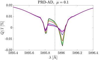
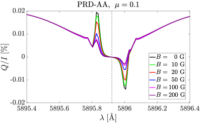
Figure 4: Emergent $Q/I$ profiles for the Na i D₁ line at $\mu=0.1$, calculated in atmospheric model C of Fontenla et al. (1993), in the presence of a microturbulent magnetic field of various strengths, taking PRD effects into account both in the general AD case (upper panel) and under the AA approximation (lower panel), in both cases neglecting the impact of $J$-state interference. The vertical dashed line indicates the line-center wavelength.

5 Conclusions

In the last years, theoretical investigations have demonstrated that the enigmatic linear polarization patterns observed in the core of the Na i D₁ line are a consequence of the variation of the anisotropy of the radiation field in the wavelength interval spanned by the line’s various HFS components (see Belluzzi & Trujillo Bueno, 2013; Belluzzi et al., 2015; Alsina Ballester et al., 2021). Because of the high computational cost of the general PRD–AD calculations, the simplifying AA assumption was made in the works mentioned above. Although this approximation is justified for modeling the intensity of spectral lines, it has been found to introduce inaccuracies in the core region of the linear polarization profiles of certain strong resonance lines (e.g., Janett et al., 2021a). In this work, we investigated the suitability of PRD–AA calculations for modeling the scattering polarization of the Na i D lines, using a numerical NLTE RT code for polarized radiation. The code is suitable for 1D atmospheric models and treats the spectral lines as arising from a two-level atomic model with HFS (i.e., neglecting the impact of $J$-state interference), accounting for isotropic microturbulent magnetic fields in the incomplete Paschen-Back effect regime.

Considering the semi-empirical atmospheric model C of Fontenla et al. (1993), we first compared the D₁ linear polarization profiles obtained under PRD–AA and PRD–AD calculations. In the absence of magnetic fields, the AD calculations yield D₁ scattering polarization amplitudes of the order of $0.01\%$, while confirming that this signal originates from the detailed spectral structure of the radiation field (see Belluzzi & Trujillo Bueno, 2013). However, the shape of the linear polarization profiles obtained under the PRD–AA and PRD–AD calculations is markedly different. A largely antisymmetric two-peak profile is found in the AA case, with a positive peak to the blue of the D₁ line center and a negative peak to the red of it, whereas a far more symmetric three-peak profile is obtained from the PRD–AD calculation, with a positive peak near the line center and a negative peak at either side of it. The PRD–AD profile also exhibits an interesting behavior with the LOS. Its central peak, shifted towards the blue for $\mu=0.1$, approaches the line center for larger $\mu$ values. As $\mu$ increases, the amplitudes of its three peaks grow until reaching a maximum and then fall.

In the presence of isotropic microturbulent magnetic fields, the sensitivity of the linear polarization profiles is quite similar for the PRD–AA and PRD–AD calculations, at least in relative terms. The signal is appreciably depolarized in the presence of magnetic fields of around $10$ G and, for stronger fields, its amplitude further reduces until about $200$ G, when saturation is reached. Nevertheless, it is worth noting that the various peaks obtained in the PRD–AD calculation are depolarized to a slightly different extent by the magnetic field.

Some impact of PRD–AD effects is also appreciable in the D₂ line-core $Q/I$ signal, where the dip feature found in the AA case is no longer obtained when such approximation is relaxed (see Figure 6). Nevertheless, the relative impact on the linear polarization amplitude is quite minor and we find a very similar magnetic sensitivity for the PRD–AA and PRD–AD cases. Because the HFS separation of the upper level of the D₂ line is smaller than that of the upper level of D₁, the D₂ linear polarization is sensitive to weaker magnetic fields; a depolarization is appreciable for strengths as low as $2$ G and saturation is found beyond roughly $100$ G.

The remarkable influence of the general PRD–AD treatment on the shape of the Na i D₁ scattering polarization pattern suggests that fully accounting for the angle-frequency coupling is crucial in explaining spectro-polarimetric observations of this line, especially those that present a rather symmetric $Q/I$ pattern. Indeed, it should be expected that the astounding variety of linear polarization patterns that are observed in this line may be partly explained by phenomena that are intrinsically linked to the three-dimensional complexity of the solar atmosphere, including horizontal inhomogeneities in its thermodynamical properties, such as temperature or density, and velocity gradients (e.g., Jaume Bestard et al., 2021). A very important goal for the near future is to model the D₁ and D₂ lines together, also accounting for PRD–AD effects and magnetic fields of arbitrary strength and orientation, considering a two-term atomic model with HFS, thus considering also $J$-state interference. This would allow us to perform a quantitative comparison with recent spectro-polarimetric observations, which revealed a wide variety of both nearly symmetric and antisymmetric $Q/I$ profiles of D₁ (e.g., Bianda et al., 2019). In any case, the results presented in this work bring us one step forward towards the goal of fully exploiting the Na i lines for diagnostics of the elusive magnetic fields of the lower solar chromosphere.

Acknowledgements: We gratefully acknowledge the financial support from the Sinergia program of the SNSF (grant No. CRSII5_180238) and from the European Research Council (ERC) under the European Union’s Horizon 2020 research and innovation program (ERC Advanced grant agreement No. 742265). T.P.A.’s participation in the publication is part of the Project RYC2021-034006-I, funded by MICIN/AEI/10.13039/501100011033, and the European Union “NextGenerationEU”/RTRP.

Appendix A Redistribution matrix for a two-level atom with HFS

The redistribution matrix for a two-level atom with HFS in the incomplete Paschen-Back effect regime for the HFS is formally equivalent to the one for a two-term atom (without HFS) in the Paschen-Back effect regime for FS, after making the appropriate substitutions discussed below. However, after these substitutions, there are certain differences between the atomic Hamiltonians of the two modelings in the presence of a magnetic field, which impact the resulting eigenvalues and eigenvectors (i.e., the energies of the atomic states and their expansion coefficients, respectively). These differences are essential to accurately account for the magnetic sensitivity of the D₁ and D₂ lines.

A.1 Two-term atom

When the magnetic splitting is comparable to the splitting between FS levels, the incomplete Paschen-Back effect regime is attained and the total electronic angular momentum $J$ is no longer a good quantum number for the atomic system. The redistribution matrix (including both $R^{\scriptscriptstyle\rm II}$ and $R^{\scriptscriptstyle\rm III}$) for a two-term atom in the Paschen-Back effect regime for the FS is given by Equation (A1) of Bommier (2017). Following the notation of that paper, the eigenvectors of the total Hamiltonian, which have the form $\ket{\beta LSJ^{\ast}M}$, can be expressed in the basis of the eigenvectors of the total angular momentum as (see Eq. (3.58) of Landi Degl’Innocenti & Landolfi, 2004)

$$\ket{\beta LSJ^{\ast}M}=\sum_{J}C^{J}_{J^{\ast}M}(B)\ket{\beta LSJM},$$ (A1)

where $\beta$ is a set of inner quantum numbers of the system, $L$ is the quantum number for orbital angular momentum, $S$ is the spin quantum number, and $M$ is the magnetic quantum number (i.e., the projection of $\bm{J}$ onto the selected quantization axis). The modified number $J^{\ast}$ indicates the angular momentum number $J$ of the corresponding atomic state in the absence of magnetic fields. The energies of the levels $\ket{\beta LSJ^{\ast}M}$ and the expansion coefficients $C^{J}_{J^{\ast}M}(B)$ are calculated through the diagonalization of the atomic Hamiltonian. Its matrix elements are

$$\bra{\beta LSJM}H_{\rm{so}}+H_{B}\ket{\beta LSJ^{\prime}M},$$ (A2)

where $H_{\rm{so}}$ and $H_{B}$ are the spin-orbit and magnetic Hamiltonian, respectively. For the magnetic fields typically found in astrophysical plasmas one can take $H_{B}=\mu_{0}\,(\bm{J}+2\bm{L})\,\bm{B}$, where $\mu_{0}$ is the Bohr magneton. By assuming that the atomic system is described by L–S coupling and applying the Wigner-Eckart theorem and its corollaries, one finds that the only non-zero matrix elements are (see Equations (3.61a) and (3.61b) of Landi Degl’Innocenti & Landolfi, 2004)

$$\bra{\beta LSJM}H_{\rm{so}}+H_{B}\ket{\beta LSJM}=E_{\beta LS}(J)+\mu_{0}Bg_{LS}(J)M,$$ (A3)

where $E_{\beta LS}(J)$ is the energy of the $J$-level and $g_{LS}(J)$ its Landé factor (see Equation (3.8) of Landi Degl’Innocenti & Landolfi, 2004)

$$g_{LS}(J)=1+\frac{1}{2}\frac{J(J+1)+S(S+1)-L(L+1)}{J(J+1)}\qquad(J\neq 0),$$ (A4)

and

$$\bra{\beta LSJ-1\,M}H_{\rm{so}}+H_{B}\ket{\beta LSJM}=\bra{\beta LSJM}H_{\rm{so}}+H_{B}\ket{\beta LSJ-1\,M}$$

$$=-\frac{\mu_{0}B}{2J}\sqrt{\frac{(J+S+L+1)(J-S+L)(J+S-L)(-J+S+L+1)(J^{2}-M^{2})}{(2J+1)(2J-1)}}.$$ (A5)

A.2 Two-level atom with HFS

The redistribution matrix for a two-level atom with HFS is still given by Equation (A.1) of Bommier (2017), with the following formal substitutions (see Equation (7.64) of Landi Degl’Innocenti & Landolfi, 2004)

$$\beta\rightarrow\alpha\qquad S\rightarrow I\qquad J^{\ast}\rightarrow F^{\ast}$$

$$L\rightarrow J\qquad J\rightarrow F\qquad M\rightarrow f,$$ (A6)

where $\alpha$ is a set of inner quantum numbers that includes $S$ and $L$, $I$ is the quantum number for nuclear spin, $F$ is the quantum number for total atomic angular momentum such that $\bm{F}=\bm{J}+\bm{I}$, and $f$ is the projection of $\bm{F}$ upon the selected quantization axis. The number $F^{\ast}$ indicates the angular momentum number $F$ of the corresponding atomic state in the absence of magnetic fields. The eigenvectors of the total Hamiltonian, which have the form $\ket{\alpha JIF^{\ast}f}$, can be expanded on the basis of the eigenvectors of the total angular momentum as (see Equation (7.58) of Landi Degl’Innocenti & Landolfi, 2004)

$$\ket{\alpha JIF^{\ast}f}=\sum_{F}C^{F}_{F^{\ast}f}(B)\ket{\alpha JIFf}.$$ (A7)

In this work, we calculate the energies of the levels $\ket{\alpha JIF^{\ast}f}$ and the expansion coefficients $C^{F}_{F^{\ast}f}(B)$ through the diagonalization of the atomic Hamiltonian, whose elements are

$$\bra{\alpha JIFf}H_{\rm{HFS}}+H_{B}\ket{\alpha JIF^{\prime}f},$$ (A8)

where $H_{\rm{HFS}}$ and $H_{B}$ are the HFS and magnetic Hamiltonian, respectively. The contribution from $H_{\rm{HFS}}$ is obtained following Equation (3.70) of Landi Degl’Innocenti & Landolfi (2004). As in the case for the two-term atom, the contribution from $H_{B}$ is obtained from the application of the Wigner-Eckart theorem and its corollaries (see Equations (3.71) and (3.73) of Landi Degl’Innocenti & Landolfi, 2004). One finds that the only non-zero matrix elements are

$$\bra{\alpha JIFf}H_{\rm{HFS}}+H_{B}\ket{\alpha JIFf}=E_{\alpha JI}(F)+\mu_{0}B\,g_{LS}(J)\,g_{\rm{HFS}}(F)\,f,$$ (A9)

where

$$E_{\alpha JI}(F)=E_{\beta LS}(J)+\frac{\mathcal{A}(\alpha,J,I)}{2}K+\mathcal{B}(\alpha,J,I)\left[K(K+1)-\frac{4}{3}J(J+1)I(I+1)\right],$$ (A10)

with $\mathcal{A}$ and $\mathcal{B}$ the HFS constants, $K=F(F+1)-J(J+1)-I(I+1)$,

$$g_{\rm{HFS}}(F)=\frac{1}{2}\frac{F(F+1)+J(J+1)-I(I+1)}{F(F+1)}\qquad(F\neq 0),$$ (A11)

and

$$\bra{\alpha JIF-1\,f} H_{\rm{HFS}}+H_{B}\ket{\alpha JIFf}=\bra{\alpha JIFf}H_{\rm{HFS}}+H_{B}\ket{\alpha JIF-1\,f}$$

$$=\mu_{0}Bg_{LS}(J)(-1)^{J+I-f}\sqrt{J(J+1)(2J+1)(2F+1)(2F-1)}\left\{\begin{array}[]{ccc}F-1&F&1\\ J&J&I\end{array}\right\}\left(\begin{array}[]{ccc}F&F-1&1\\ -f&f&0\end{array}\right)$$ (A16)

$$=\frac{\mu_{0}Bg_{LS}(J)}{2F}\sqrt{\frac{(F+J+I+1)(F-I+J)(F+I-J)(-F+J+I+1)(F^{2}-f^{2})}{(2F+1)(2F-1)}}.$$ (A17)

In this work, we compute the eigenvectors and eigenvalues of the atomic Hamiltonian by considering the matrix elements given in Equations (A9) and (A17). We note that these elements are not equivalent to the analogous ones for the two-term atom without HFS obtained via the formal substitutions shown in Equations (A6). The contribution from the magnetic Hamiltonian in Equation (A9) differs from the one that would be obtained from Equation (A3) in the $g_{LS}(J)\,g_{\rm{HFS}}(F)$ factor of the former. In addition, the element in Equation (A17) differs from the one that would be obtained from Equation (A5) in the overall sign and in the $g_{LS}(J)$ factor.

Appendix B Impact of PRD–AD treatment on D₂ polarization

In this section, we analyze the suitability of a PRD–AA modeling for the Na i D₂ line at 5890 Å, through quantitative comparisons with the general PRD–AD calculations, both in the absence and presence of magnetic fields. We considered the same setting exposed in Section 4.1 and the wavelength interval $[\lambda_{\min},\lambda_{\max}]=[5887.3\text{\,\AA},5892.6\text{\,\AA}]$. Figure 5 compares the $Q/I$ patterns of the D₂ line obtained for PRD–AA and for PRD–AD calculations at $\mu=\cos(\theta)=0.1$ and in the absence of magnetic fields. The left and right panels of Figure 6 show the $Q/I$ patterns obtained from AD and AA calculations, respectively, at $\mu=\cos(\theta)=0.1$. In these calculations, we accounted for isotropic microturbulent magnetic fields of various strengths, ranging from $0$ to $10$ G, for which the incomplete Paschen-Back effect regime must be considered. Under the PRD–AA approximation, the $Q/I$ profile of the D₂ line presents an artificial dip in its core, which is not found for the PRD–AD case. This result is similar to what was reported in an analogous investigation on the Ca i line at $4227$ Å by Janett et al. (2021a). However, the relative impact on the linear polarization amplitude is quite minor when compared to the Na i D₁ case. Moreover, we find a very similar magnetic sensitivity for the PRD–AA and PRD–AD cases.

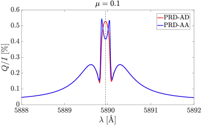
Figure 5: Emergent $Q/I$ profiles for the Na i D₂ line at $\mu=0.1$, calculated with a two-level model atom and in the atmospheric model C of Fontenla et al. (1993), without a magnetic field. The results of calculations are shown taking PRD effects into account both in the general AD case (red curve) and under the AA approximation (blue curve). The vertical dashed line indicates the line-center wavelength.

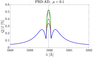
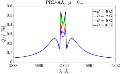
Figure 6: Emergent $Q/I$ profiles for the Na i D₂ line at $\mu=0.1$, calculated in atmospheric model C of Fontenla et al. (1993), in the presence of a microturbulent magnetic field of various strengths, taking PRD effects into account both in the general AD case (left panel) and under the AA approximation (right panel). The vertical dashed line indicates the line-center wavelength.

Appendix C Angular sampling

For the angular discretization of $\bm{\Omega}=(\theta,\chi)$, we use a tensor product quadrature. For the inclination $\mu=\cos(\theta)\in[-1,1]$, we consider two Gauss-Legendre grids (and corresponding weights) for $\mu\in(-1,0)$ and $\mu\in(0,1)$, respectively, with $N_{\theta}/2$ nodes each, namely

$$1>\mu_{1}>\mu_{2}>\cdots>\mu_{N_{\theta}/2}>0>\mu_{N_{\theta}/2+1}>\cdots>\mu_{N_{\theta}}>-1.$$

This grid corresponds to

$$0<\theta_{1}<\theta_{2}<\cdots<\theta_{N_{\theta}/2}<\pi/2<\theta_{N_{\theta}/2+1}<\cdots<\theta_{N_{\theta}}<\pi,$$

with $\theta_{j}=\arccos(\mu_{j})$ for $j=1,\ldots,N_{\theta}$, with $N_{\theta}$ even. For the azimuth $\chi\in(0,2\pi]$, we consider an equidistant grid (and corresponding trapezoidal weights) with $N_{\chi}$ nodes, namely

$$\chi_{k}=k\cdot 2\pi/N_{\chi}\quad\text{for}\quad k=1,\ldots,N_{\chi}.$$

Figure 7 presents the emergent $Q/I$ profiles for the Na i D₁ line obtained with PRD–AD calculations in the absence of magnetic fields with $N_{\theta}=12$ at $\mu=0.17$ (left panel) and $N_{\theta}=24$ at $\mu=0.21$ (right panel) for various azimuthal samplings. The two panels are shown for different LOSs, so that they lie on the considered angular grid. For both $N_{\theta}=12,24$, the very common azimuthal sampling given by $N_{\chi}=8$ was revealed to be inaccurate for modeling these scattering polarization signals, taking PRD effects into account in the general AD case. Therefore, we set $N_{\chi}=12$ in all the AD calculations shown in this work.

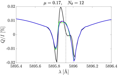
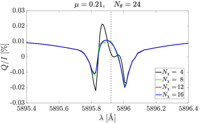
Figure 7: Emergent $Q/I$ profiles for the Na i D₁ line obtained through the PRD calculations detailed in the main text in the general AD case. Model C of Fontenla et al. (1993) was considered in the absence of magnetic fields. The vertical dashed line indicates the line-center wavelength. The results of calculations are shown for angular grids with $N_{\chi}=4,8,12,16$ (see legend) and with $N_{\theta}=12$ at $\mu=0.17$ (left panel) and $N_{\theta}=24$ at $\mu=0.21$ (right panel). All the results shown in this work were thus obtained considering $N_{\chi}=12$ and $N_{\theta}=12$.

Appendix D Frequency-integrated D₁ linear polarization signal

Figure 8 shows the frequency-integrated $\overline{Q}$ signals of the Na i D₁ line, normalized to the continuum intensity $I_{c}$, as a function of $\mu$. It presents a comparison between the signals obtained from calculations taking PRD effects into account in the general AD case and under the AA approximation in the absence of magnetic fields, neglecting the continuum contribution to polarization. We note that the amplitudes in the AD curve are comparable to those in the AA one, indicating that the AD treatment does not lead to an enhancement of the net $\overline{Q}/I_{c}$ signal. In addition, we computed the emergent $\overline{Q}/\overline{I}$ ratio in a frequency interval corresponding to $\pm 0.50$ Å from the line center. We found the largest values for $\overline{Q}/\overline{I}$ to be on the order of $10^{-5}$, for $\mu$ positions close to the limb. The largest contribution to the net linear polarization comes from the regions between $\sim\!0.15$ and $\sim\!0.40$ Å from the line center, both to the red and the blue, where Stokes $Q$ signals of the same sign are found. Such wing signals arise mainly as a consequence of transfer effects. To verify this, we computed the $\overline{\varepsilon}_{Q}/\overline{\varepsilon}_{I}$ ratio for the AA case, neglecting continuum contributions, at all height points between $600$ and $2017$ km in the FAL-C atmospheric model. The largest value of $\overline{\varepsilon}_{Q}/\overline{\varepsilon}_{I}$, found for $\mu$ positions close to the limb, is on the order of $10^{-6}$, that is one order of magnitude smaller than the emergent $\overline{Q}/\overline{I}$ ratio.

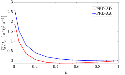
Figure 8: Frequency-integrated emergent $\overline{Q}/I_{c}$ signals as a function of $\mu$ for the Na i D₁ line, calculated in atmospheric model C of Fontenla et al. (1993) in the absence of magnetic fields. The signals were obtained from the profiles calculated neglecting the continuum contribution to polarization and taking PRD effects into account both in the general AD case (red curve) and under the AA approximation (blue curve), for an angular grid with $N_{\chi}=12$ and $N_{\theta}=24$.

References

- Alsina Ballester (2022) Alsina Ballester, E. 2022, A&A, 666, A178
- Alsina Ballester et al. (2017) Alsina Ballester, E., Belluzzi, L., & Trujillo Bueno, J. 2017, ApJ, 836, 6
- Alsina Ballester et al. (2021) Alsina Ballester, E., Belluzzi, L., & Trujillo Bueno, J. 2021, Phys. Rev. Lett., 127, 081101
- Alsina Ballester et al. (2022) Alsina Ballester, E., Belluzzi, L., & Trujillo Bueno, J. 2022, A&A, 664, A76
- Anusha (2023) Anusha, L. S. 2023, ApJ, 949, 84
- Belluzzi & Trujillo Bueno (2013) Belluzzi, L. & Trujillo Bueno, J. 2013, ApJ, 774, L28
- Belluzzi & Trujillo Bueno (2014) Belluzzi, L. & Trujillo Bueno, J. 2014, A&A, 564, A16
- Belluzzi et al. (2015) Belluzzi, L., Trujillo Bueno, J., & Landi Degl’Innocenti, E. 2015, ApJ, 814, 116
- Benedusi et al. (2021) Benedusi, P., Janett, G., Belluzzi, L., & Krause, R. 2021, A&A, accepted
- Benedusi et al. (2022) Benedusi, P., Janett, G., Riva, S., Krause, R., & Belluzzi, L. 2022, A&A, 664, A197
- Benedusi et al. (2023) Benedusi, P., Riva, S., Zulian, P., et al. 2023, Journal of Computational Physics, 479, 112013
- Bianda et al. (2019) Bianda, M., Ramelli, R., Gisler, D., Belluzzi, L., & Carlin, E. S. 2019, in Astronomical Society of the Pacific Conference Series, Vol. 526, Solar Polariation Workshop 8, ed. L. Belluzzi, R. Casini, M. Romoli, & J. Trujillo Bueno, 223
- Bommier (1997) Bommier, V. 1997, A&A, 328, 726
- Bommier (2017) Bommier, V. 2017, A&A, 607, A50
- Bommier (2018) Bommier, V. 2018, A&A, 619, C1
- Faurobert (1987) Faurobert, M. 1987, A&A, 178, 269
- Faurobert (1988) Faurobert, M. 1988, A&A, 194, 268
- Fontenla et al. (1991) Fontenla, J. M., Avrett, E. H., & Loeser, R. 1991, ApJ, 377, 712
- Fontenla et al. (1993) Fontenla, J. M., Avrett, E. H., & Loeser, R. 1993, ApJ, 406, 319
- Gandorfer (2002) Gandorfer, A. 2002, The Second Solar Spectrum: Volume II (Hochschulverlag AG, ETHZ)
- Hummer (1962) Hummer, D. G. 1962, MNRAS, 125, 21
- Janett et al. (2021a) Janett, G., Alsina Ballester, E., Guerreiro, N., et al. 2021a, A&A, 655, A13
- Janett et al. (2021b) Janett, G., Benedusi, P., Belluzzi, L., & Krause, R. 2021b, A&A, 655, A87
- Janett et al. (2017) Janett, G., Carlin, E. S., Steiner, O., & Belluzzi, L. 2017, ApJ, 840, 107
- Janett & Paganini (2018) Janett, G. & Paganini, A. 2018, ApJ, 857, 91
- Janett et al. (2018) Janett, G., Steiner, O., & Belluzzi, L. 2018, ApJ, 865, 16
- Jaume Bestard et al. (2021) Jaume Bestard, J., Trujillo Bueno, J., Štěpán, J., & del Pino Alemán, T. 2021, ApJ, 909, 183
- Kerkeni & Bommier (2002) Kerkeni, B. & Bommier, V. 2002, A&A, 394, 707
- Kramida et al. (2022) Kramida, A., Yu. Ralchenko, Reader, J., & and NIST ASD Team. 2022, NIST Atomic Spectra Database (ver. 5.10), [Online]. Available: https://physics.nist.gov/asd [2023, May 8]. National Institute of Standards and Technology, Gaithersburg, MD.
- Landi Degl’Innocenti (1998) Landi Degl’Innocenti, E. 1998, Nature, 392, 256
- Landi Degl’Innocenti & Landolfi (2004) Landi Degl’Innocenti, E. & Landolfi, M. 2004, Astrophysics and Space Science Library, Vol. 307, Polarization in Spectral Lines (Dordrecht: Kluwer Academic Publishers)
- Leenaarts et al. (2012) Leenaarts, J., Pereira, T., & Uitenbroek, H. 2012, A&A, 543, A109
- Manso Sainz et al. (2004) Manso Sainz, R., Landi Degl’Innocenti, E., & Trujillo Bueno, J. 2004, The Astrophysical Journal, 614, L89
- Mihalas (1978) Mihalas, D. 1978, Stellar Atmospheres, 2nd edn. (San Francisco: W.H. Freeman and Company)
- Nagendra et al. (2020) Nagendra, K. N., Sowmya, K., Sampoorna, M., Stenflo, J. O., & Anusha, L. S. 2020, ApJ, 898, 49
- Rees & Saliba (1982) Rees, D. E. & Saliba, G. J. 1982, A&A, 115, 1
- Sampoorna (2014) Sampoorna, M. 2014, in Astronomical Society of the Pacific Conference Series, Vol. 489, Solar Polarization 7, ed. K. N. Nagendra, J. O. Stenflo, Z. Q. Qu, & M. Sampoorna, 197
- Sampoorna & Nagendra (2016) Sampoorna, M. & Nagendra, K. N. 2016, ApJ, 833, 32
- Sampoorna et al. (2011) Sampoorna, M., Nagendra, K. N., & Frisch, H. 2011, A&A, 527, A89
- Sampoorna et al. (2019) Sampoorna, M., Nagendra, K. N., Sowmya, K., Stenflo, J. O., & Anusha, L. S. 2019, ApJ, 883, 188
- Sampoorna et al. (2017) Sampoorna, M., Nagendra, K. N., & Stenflo, J. O. 2017, ApJ, 844, 97
- Steck (2003) Steck, D. A. 2003, Sodium D Line Data. Notes available at http://steck.us/alkalidata
- Stenflo (1994) Stenflo, J. 1994, Solar Magnetic Fields: Polarized Radiation Diagnostics, Vol. 189 (Springer)
- Stenflo & Keller (1997) Stenflo, J. O. & Keller, C. U. 1997, A&A, 321, 927
- Trujillo Bueno (2001) Trujillo Bueno, J. 2001, in Astronomical Society of the Pacific Conference Series, Vol. 236, Advanced Solar Polarimetry – Theory, Observation, and Instrumentation, ed. M. Sigwarth, 161
- Trujillo Bueno & del Pino Alemán (2022) Trujillo Bueno, J. & del Pino Alemán, T. 2022, ARA&A, 60, 415
- Trujillo Bueno & Manso Sainz (1999) Trujillo Bueno, J. & Manso Sainz, R. 1999, ApJ, 516, 436
- Trujillo Bueno et al. (2004) Trujillo Bueno, J., Shchukina, N., & Asensio Ramos, A. 2004, Nature, 430, 326