A second-order in time, BGN-based parametric finite element method for geometric flows of curves

Abstract

Over the last two decades, the field of geometric curve evolutions has attracted significant attention from scientific computing. One of the most popular numerical methods for solving geometric flows is the so-called BGN scheme, which was proposed by Barrett, Garcke, and Nürnberg (J. Comput. Phys., 222 (2007), pp. 441–467), due to its favorable properties (e.g., its computational efficiency and the good mesh property). However, the BGN scheme is limited to first-order accuracy in time, and how to develop a higher-order numerical scheme is challenging. In this paper, we propose a fully discrete, temporal second-order parametric finite element method, which incorporates a mesh regularization technique when necessary, for solving geometric flows of curves. The scheme is constructed based on the BGN formulation and a semi-implicit Crank-Nicolson leap-frog time stepping discretization as well as a linear finite element approximation in space. More importantly, we point out that the shape metrics, such as manifold distance and Hausdorff distance, instead of function norms, should be employed to measure numerical errors. Extensive numerical experiments demonstrate that the proposed BGN-based scheme is second-order accurate in time in terms of shape metrics. Moreover, by employing the classical BGN scheme as a mesh regularization technique when necessary, our proposed second-order scheme exhibits good properties with respect to the mesh distribution.

1 Introduction

Geometric flows, which describe the evolution of curves or surfaces over time based on the principle that the shape changes according to its underlying geometric properties, such as the curvature, have been extensively studied in the fields of computational geometry and geometric analysis. In particular, second-order (e.g., mean curvature flow, which is also called as curve-shortening flow for curve evolution) and fourth-order (e.g., surface diffusion flow) geometric flows have attracted considerable interest due to their wide-ranging applications in materials science [6, 31], image processing [1], multiphase fluids [21] and cell biology [13]. For more in-depth information, readers can refer to the recent review articles [14, 17], and references provided therein.

In this paper, we focus on three different types of geometric flows of curves: curve-shortening flow (CSF), area-preserving curve-shortening flow (AP-CSF) and surface diffusion flow (SDF). First, assume that $\Gamma(t)$ is a family of simple closed curves in the two-dimensional plane. We consider that the curve is governed by the three geometric flows, i.e., its velocity is respectively given by

$${\mathcal{V}}=\begin{cases}-\kappa\mathbf{n},&\quad\text{CSF},\\ (-\kappa+\left<\kappa\right>)\mathbf{n},&\quad\text{AP-CSF},\\ (\partial_{ss}\kappa)\mathbf{n},&\quad\text{SDF},\end{cases}$$ (1.1)

where $\kappa$ is the curvature of the curve, $s$ is the arc-length, $\left<\kappa\right>:=\int_{\Gamma(t)}\kappa\mathrm{d}s/\int_{\Gamma(t)}1\mathrm{d}s$ is the average curvature and $\mathbf{n}$ is the outward unit normal to $\Gamma$. Here, we use the sign convention that a unit circle has a positive constant curvature.

By representing the curves $\Gamma(t)$ as a parametrization $\mathbf{X}(\cdot,t):\mathbb{I}\rightarrow{\mathbb{R}}^{2}$, where $\mathbb{I}:=\mathbb{R}/\mathbb{Z}$ is the “periodic” interval $[0,1]$, Barrett, Garcke and Nürnberg [10, 14] creatively reformulated the above equations (1.1) into the following coupled forms:

$$\begin{split}\partial_{t}\mathbf{X}\cdot\mathbf{n}&=\begin{cases}-\kappa,&\quad\text{CSF},\\ -\kappa+\left<\kappa\right>,&\quad\text{AP-CSF},\\ \partial_{ss}\kappa,&\quad\text{SDF},\end{cases}\\ \kappa\mathbf{n}&=-\partial_{ss}\mathbf{X}.\end{split}$$ (1.2)

Based on the above equations and the corresponding weak formulations, a series of numerical schemes (the so-called BGN schemes) were proposed for solving different geometric flows, such as mean curvature flow and surface diffusion [10, 11], Willmore flow [13], anisotropic geometric flow [5], solid-state dewetting [6, 31] and geometric flow for surface evolution [12]. Recently, based on the BGN formulation (1.2), structure-preserving schemes have been proposed for axisymmetric geometric equations [4] and surface diffusion [7, 5], respectively. In practical simulations, ample numerical results have demonstrated the high performance of the BGN scheme, due to inheriting the variational structure of the original problem and introducing an appropriate tangential velocity to help mesh points maintain a good distribution. However, for the original BGN scheme, because its formal truncation error is $\mathcal{O}(\tau)$, where $\tau$ is the time step size, the temporal convergence order of the scheme is limited to the first-order. This has been confirmed by extensive numerical experiments [7, 10, 11, 6]. Therefore, how to design a temporal high-order scheme which is based on the BGN formulation (1.2) is challenging and still open. It is also worth noting that rigorous numerical analysis for BGN schemes remains an open problem [14].

In this paper, based on the BGN formulation (1.2), we propose a novel temporal second-order parametric finite element method for solving geometric flows of curves, i.e., CSF, AP-CSF and SDF. Specifically, to discretize the same continuous-in-time semi-discrete formulation as the classical BGN scheme [10], we begin by fixing the unit normal as that on the current curve $\Gamma^{m}$ and then discretize other terms using the Crank-Nicolson leap-frog scheme [22]. The resulting scheme is a second-order semi-implicit scheme, which only requires solving a system of linear algebraic equations at each time step. Furthermore, the well-posedness and mild energy stability of the fully discrete scheme can be established under suitable assumption conditions. Numerical results have demonstrated that the proposed scheme achieves second-order accuracy in time, as measured by the shape metrics, outperforming the classical BGN scheme in terms of accuracy and efficiency.

It is worth mentioning that there exist several temporal higher-order numerical schemes based on other formulations which have been proposed for simulating geometric flows. For the specific case of curve-shortening flow, a Crank-Nicolson-type scheme combined with tangential redistribution [3] and an adaptive moving mesh method [28] have been developed. Both of the schemes are convergent quadratically in time and fully implicit, requiring to solve a system of nonlinear equations at each time step. Recently, an evolving surface finite element method together with linearly implicit backward difference formulae for time integration for simulating the mean curvature flow has been proposed in [26, 27]. In comparison to these existing approaches, our newly proposed scheme is based on the BGN formulation (1.2), then it inherits the variational structure of the original geometric flows, and has very good property with respect to mesh distribution. The new scheme exhibits comparable computational cost to the classical BGN scheme while surpassing it in terms of accuracy. Furthermore, it can be extended easily to other geometric flows with applications to various fields.

The main reason why we have successfully proposed a temporal high-order, BGN-based parametric finite element method for solving geometric flows lies in the following two key points: (1). we choose an appropriate metric (i.e., shape metrics) to measure numerical errors of the proposed schemes; (2). we use the classical first-order BGN scheme as “a good partner” of the proposed scheme to help mesh points maintain a good distribution without sacrificing the accuracy.

How to measure the errors of numerical solutions for geometric flows is an important issue. A natural approach is to use classical Sobolev norms, such as $L^{2}$-norm, $L^{\infty}$-norm or $H^{1}$-norm, which are widely used in the numerical analysis for geometric flows [18, 19, 26, 27]. However, when it comes to numerical schemes that involve in tangential movements, these function norms may not be suitable for quantifying the differences between two curves/surfaces. To address this issue, we consider an alternative approach using shape metrics, such as manifold distance (as used in [7, 32]) and Hausdorff distance [2]. These metrics provide a measure of how similar or different two curves/surfaces are in terms of their shape characteristics. Extensive numerical experiments have been conducted, and the results demonstrate that our proposed scheme achieves second-order accuracy when measured using shape metrics.

On the other hand, the quality of mesh distribution is always a major concern when simulating geometric flows using parametric finite element methods. It is important to note that the original flow (1.1) requires the curve to evolve only in the normal direction, thus the numerical methods based on (1.1) which prevent tangential movement of mesh points might lead to mesh distortion or clustering during the evolution. To address this issue, various approaches have been proposed in the literature to maintain good mesh quality, e.g., artificial mesh regularization method [15], reparametrization by introducing a tangential velocity [16, 29, 20, 25, 30]. On the contrary, the BGN formulation (1.2) does not enforce any condition on the tangential velocity, which allows for an intrinsic tangential motion of mesh points, as demonstrated by the standard BGN scheme [10, 11] constructed based on this formulation (1.2). Though the semi-discrete scheme of (1.2), where only spatial discretization is performed, results in precise equidistribution of mesh points, our proposed fully discrete second-order BGN-based scheme exhibits oscillations in terms of mesh ratio and other geometric quantities, which may lead to instability in certain situations. To overcome this problem, we employ the classical first-order BGN scheme as a mesh regularization procedure to improve mesh quality once poorly distributed polygonal approximations are observed. Extensive numerical experiments indicate that this mesh regularization remedy enhances the stability of the new scheme and improves mesh quality significantly. Fortunately, numerous numerical experiments have also demonstrated that this mesh regularization only occurs a few times during the evolution, thus not compromising the temporal second-order accuracy of the proposed scheme.

The remaining of the paper is organized as follows. In Section 2, taking CSF as an example, we begin by recalling the standard BGN scheme, and then propose a second-order in time, BGN-based parametric finite element method for solving CSF. Section 3 is devoted to explaining the importance of using shape metrics, such as manifold distance and Hausdorff distance, to accurately measure the errors of two curves. We extend the proposed second-order scheme to other geometric flows such as AP-CSF and the fourth-order flow SDF in Section 4. Extensive numerical results are provided to demonstrate the accuracy and efficiency of the proposed schemes in Section 5. Finally, we draw some conclusions in Section 6.

2 For curve shortening flow (CSF)

In this section, we propose a parametric finite element method with second-order temporal accuracy for numerically solving the CSF. The same idea can be easily extended to other geometric flows (cf. Section 4). To provide a comprehensive understanding, we first review the classical first-order BGN scheme proposed by Barrett, Garcke and Nürnberg [10, 11, 14].

2.1 Weak formulation and BGN scheme

To begin with, we rewrite the CSF into the following formulation as presented in Eqs. (1.2):

$$\begin{split}\partial_{t}\mathbf{X}\cdot\mathbf{n}&=-\kappa,\\ \kappa\mathbf{n}&=-\partial_{ss}\mathbf{X}.\end{split}$$ (2.1)

We introduce the following finite element approximation. Let $\mathbb{I}=[0,1]=\bigcup_{j=1}^{N}I_{j}$, $N\geq 3$, be a decomposition of $\mathbb{I}$ into intervals given by the nodes $q_{j}$, $I_{j}=[\rho_{j-1},\rho_{j}]$. Let $h=\max\limits_{1\leq j\leq N}|\rho_{j}-\rho_{j-1}|$ be the maximal length of a grid element. Define the linear finite element space as

$$V^{h}:=\{u\in C(\mathbb{I}):u|_{I_{j}}\,\,\,\mathrm{is\,\,\,linear,\,\,\,}\forall j=1,2,\ldots,N;\quad u(\rho_{0})=u(\rho_{N})\}\subseteq H^{1}(\mathbb{I}).$$

The mass lumped inner product $(\cdot,\cdot)_{\Gamma^{h}}^{h}$ over the polygonal curve $\Gamma^{h}$, which is an approximation of $(\cdot,\cdot)_{\Gamma^{h}}$ by using the composite trapezoidal rule, is defined as

$$(u,v)_{\Gamma^{h}}^{h}:=\frac{1}{2}\sum_{j=1}^{N}|\mathbf{X}^{h}(\rho_{j},t)-\mathbf{X}^{h}(\rho_{j-1},t)|\left[(u\cdot v)(\rho_{j}^{-})+(u\cdot v)(\rho_{j-1}^{+})\right],$$

where $u,v$ are two scalar/vector piecewise continuous functions with possible jumps at the nodes $\{\rho_{j}\}_{j=1}^{N}$, and $u(\rho_{j}^{\pm})=\lim\limits_{\rho\rightarrow\rho_{j}^{\pm}}u(\rho)$.

Subsequently, the semi-discrete scheme of the formulation (2.1) is as follows: given initial polygon $\Gamma^{h}(0)$ with vertices lying on the initial curve $\Gamma(0)$ clockwise, parametrized by $\mathbf{X}^{h}(\cdot,0)\in[V^{h}]^{2}$, find $(\mathbf{X}^{h}(\cdot,t),\kappa^{h}(\cdot,t))\in[V^{h}]^{2}\times V^{h}$ such that

$$\begin{cases}\left(\partial_{t}\mathbf{X}^{h}\cdot\mathbf{n}^{h},\varphi^{h}\right)_{\Gamma^{h}}^{h}+\left(\kappa^{h},\varphi^{h}\right)^{h}_{\Gamma^{h}}=0,\quad\forall\ \varphi^{h}\in V^{h},\\ \left(\kappa^{h},\mathbf{n}^{h}\cdot\bm{\omega}^{h}\right)^{h}_{\Gamma^{h}}-\left(\partial_{s}\mathbf{X}^{h},\partial_{s}\bm{\omega}^{h}\right)_{\Gamma^{h}}=0,\quad\forall\ \bm{\omega}^{h}\in[V^{h}]^{2},\end{cases}$$ (2.2)

where we always integrate over the current curve $\Gamma^{h}$ described by $\mathbf{X}^{h}$, the outward unit normal $\mathbf{n}^{h}$ is a piecewise constant vector given by

$$\mathbf{n}^{h}|_{I_{j}}=-\frac{\mathbf{h}_{j}^{\perp}}{|\mathbf{h}_{j}|},\quad\mathbf{h}_{j}=\mathbf{X}^{h}(\rho_{j},t)-\mathbf{X}^{h}(\rho_{j-1},t),\quad j=1,\ldots,N,$$

with $\cdot^{\perp}$ denoting clockwise rotation by $\frac{\pi}{2}$, and the partial derivative $\partial_{s}$ is defined piecewisely over each side of the polygon $\partial_{s}f|_{I_{j}}=\frac{\partial_{\rho}f}{|\partial_{\rho}\mathbf{X}^{h}|}|_{I_{j}}=\frac{(\rho_{j}-\rho_{j-1})\partial_{\rho}f|_{I_{j}}}{|\mathbf{h}_{j}|}$. It was shown that the scheme (2.2) will always equidistribute the vertices along $\Gamma^{h}$ for $t>0$ if they are not locally parallel (see Remark 2.4 in [10]).

For a full discretization, we fix $\tau>0$ as a uniform time step size for simplicity, and let $\mathbf{X}^{m}\in[V^{h}]^{2}$ and $\Gamma^{m}$ be the approximations of $\mathbf{X}(\cdot,t_{m})$ and $\Gamma(t_{m})$, respectively, for $m=0,1,2,\ldots$, where $t_{m}:=m\tau$. We define $\mathbf{h}_{j}^{m}:=\mathbf{X}^{m}(\rho_{j})-\mathbf{X}^{m}(\rho_{j-1})$ and assume $|\mathbf{h}_{j}^{m}|>0$ for $j=1,\ldots,N$, $\forall\ m>0$. The discrete unit normal vector $\mathbf{n}^{m}$, the discrete inner product $(\cdot,\cdot)^{h}_{\Gamma^{m}}$ and the discrete operator $\partial_{s}$ are defined similarly as in the semi-discrete case. Barrett, Garcke and Nürnberg used a formal first-order approximation [10, 11] to replace the velocity $\partial_{t}\mathbf{X}$, $\kappa$ and $\partial_{s}\mathbf{X}$ by

$$\begin{split}\partial_{t}\mathbf{X}(\cdot,t_{m})&=\frac{\mathbf{X}(\cdot,t_{m+1})-\mathbf{X}(\cdot,t_{m})}{\tau}+\mathcal{O}(\tau),\\ \kappa(\cdot,t_{m})&=\kappa(\cdot,t_{m+1})+\mathcal{O}(\tau),\\ \partial_{s}\mathbf{X}(\cdot,t_{m})&=\partial_{s}\mathbf{X}(\cdot,t_{m+1})+\mathcal{O}(\tau),\end{split}$$

and the fully discrete semi-implicit BGN scheme (denoted as BGN1 scheme) reads as:

(BGN1, First-order in time BGN scheme for CSF): For $m\geq 0$, find $\mathbf{X}^{m+1}\in[V^{h}]^{2}$ and $\kappa^{m+1}\in V^{h}$ such that

$$\begin{cases}\left(\frac{\mathbf{X}^{m+1}-\mathbf{X}^{m}}{\tau},\varphi^{h}\mathbf{n}^{m}\right)^{h}_{\Gamma^{m}}+\left(\kappa^{m+1},\varphi^{h}\right)_{\Gamma^{m}}^{h}=0,\quad\forall\ \varphi^{h}\in V^{h},\\ \left(\kappa^{m+1},\mathbf{n}^{m}\cdot\bm{\omega}^{h}\right)_{\Gamma^{m}}^{h}-\left(\partial_{s}\mathbf{X}^{m+1},\partial_{s}\bm{\omega}^{h}\right)_{\Gamma^{m}}=0,\quad\forall\ \bm{\omega}^{h}\in[V^{h}]^{2}.\end{cases}$$ (2.3)

The well-posedness and energy stability were established under some mild conditions. In practice, numerous numerical results show that the BGN1 scheme (2.3) converges quadratically in space [11] and linearly in time (cf. Fig. 1 in Section 5.1).

2.2 A second-order in time, BGN-based scheme

Instead of using the first-order Euler method, we apply the Crank-Nicolson leap-frog time stepping discretization in (2.2) based on the following simple calculation

$$\begin{split}\partial_{t}\mathbf{X}(\cdot,t_{m})&=\frac{\mathbf{X}(\cdot,t_{m+1})-\mathbf{X}(\cdot,t_{m-1})}{2\tau}+\mathcal{O}(\tau^{2}),\\ \kappa(\cdot,t_{m})&=\frac{\kappa(\cdot,t_{m+1})+\kappa(\cdot,t_{m-1})}{2}+\mathcal{O}(\tau^{2}),\\ \partial_{s}\mathbf{X}(\cdot,t_{m})&=\frac{\partial_{s}\mathbf{X}(\cdot,t_{m+1})+\partial_{s}\mathbf{X}(\cdot,t_{m-1})}{2}+\mathcal{O}(\tau^{2}),\end{split}$$ (2.4)

then the corresponding second-order scheme (denoted as BGN2 scheme) is as follows:

(BGN2, Second-order in time BGN-based scheme for CSF):  For $\mathbf{X}^{0}\in[V^{h}]^{2}$, $\kappa^{0}\in V^{h}$ and $(\mathbf{X}^{1},\kappa^{1})\in[V^{h}]^{2}\times V^{h}$ which are the appropriate approximations at the time levels $t_{0}=0$ and $t_{1}=\tau$, respectively, find $\mathbf{X}^{m+1}\in[V^{h}]^{2}$ and $\kappa^{m+1}\in V^{h}$ for $m\geq 1$ such that

$$\begin{cases}\left(\frac{\mathbf{X}^{m+1}-\mathbf{X}^{m-1}}{2\tau},\varphi^{h}\mathbf{n}^{m}\right)^{h}_{\Gamma^{m}}+\left(\frac{\kappa^{m+1}+\kappa^{m-1}}{2},\varphi^{h}\right)_{\Gamma^{m}}^{h}=0,\\ \vspace{-3mm}\\ \left(\frac{\kappa^{m+1}+\kappa^{m-1}}{2},\mathbf{n}^{m}\cdot\bm{\omega}^{h}\right)_{\Gamma^{m}}^{h}-\left(\frac{\partial_{s}\mathbf{X}^{m+1}+\partial_{s}\mathbf{X}^{m-1}}{2},\partial_{s}\bm{\omega}^{h}\right)_{\Gamma^{m}}=0,\end{cases}$$ (2.5)

for all $(\varphi^{h},\bm{\omega}^{h})\in V^{h}\times[V^{h}]^{2}$. The scheme (2.5) is semi-implicit and the computational cost is comparable to that of the BGN1 scheme (2.3). Moreover, as a temporal discretization of the semi-discrete version (2.2), it can be easily derived from (2.4) that the truncation error is of order $\mathcal{O}(\tau^{2})$.

Remark 2.1.

To begin the BGN2 scheme (2.5), we need to first prepare the data $\kappa^{0}$ and $(\mathbf{X}^{1},\kappa^{1})$. In practical simulations, this can be easily achieved without sacrificing the accuracy of the scheme by utilizing the standard BGN1 scheme (2.3) to get $(\mathbf{X}^{1},\kappa^{1})$, and the following formula of discrete curvature was proposed in [10, Page 461] to prepare $\kappa^{0}$ (note the the sign convention of the curvature is opposite to [10])

$$\kappa^{0}=(N_{0}^{\top}N_{0})^{-1}N_{0}^{\top}A_{0}\textbf{X}^{0},$$ (2.6)

where $N_{0}$ is a $2N\times N$ matrix, $\textbf{X}^{0}$ is a $2N\times 1$ vector and $A_{0}$ is a $2N\times 2N$ matrix given by

$$N_{0}=\begin{pmatrix}(\varphi_{i},(\mathbf{n}^{0})^{[1]}\varphi_{j})_{\Gamma^{0}}^{h}\\ (\varphi_{i},(\mathbf{n}^{0})^{[2]}\varphi_{j})_{\Gamma^{0}}^{h}\end{pmatrix},\quad\textbf{X}^{0}=\begin{pmatrix}\textbf{x}^{0}\\ \textbf{y}^{0}\end{pmatrix},$$

$$A_{0}=\begin{pmatrix}(\partial_{s}\varphi_{i},\partial_{s}\varphi_{j})_{\Gamma^{0}}&0\\ 0&(\partial_{s}\varphi_{i},\partial_{s}\varphi_{j})_{\Gamma^{0}}\end{pmatrix},$$

where $\varphi_{i},1\leq i\leq N$ are the standard Lagrange basis over $\mathbb{I}$, and $\mathbf{a}^{[1]},\mathbf{a}^{[2]}$ are the first and second component of vector $\mathbf{a}\in{\mathbb{R}}^{2}$, and $\textbf{x}_{j}^{0}=(\mathbf{X}^{0})^{[1]}(\rho_{j})$, $\textbf{y}_{j}^{0}=(\mathbf{X}^{0})^{[2]}(\rho_{j})$ for $j=1,\ldots,N$. Note that this formula can be derived by solving the finite element approximation of the equation $\kappa\mathbf{n}=-\partial_{ss}\mathbf{X}$ and using the least square method. We can summarize the process as Algorithm 2.1, which outlines the steps to prepare the required data $\kappa^{0}$ and $(\mathbf{X}^{1},\kappa^{1})$. Once we have obtained these data, we can directly apply the BGN2 scheme (2.5) to calculate $(\mathbf{X}^{m},\kappa^{m})$, for $m\geq 2$.

Algorithm 2.1.

(Preparation for the initial data of BGN2 for CSF)

$\bm{Step~{}0.}$ Given the initial curve $\Gamma(0)$, the number of grid points $N$ and the time step size $\tau$. We choose the polygon $\Gamma^{0}$ with $N$ vertices lying on $\Gamma(0)$ such that $\Gamma^{0}$ is (almost) equidistributed, i.e., each side of the polygon is (nearly) equal in length. We parameterize $\Gamma^{0}$ with $\mathbf{X}^{0}\in[V^{h}]^{2}$ and the grid points $\rho_{j}$ can be determined correspondingly.

$\bm{Step~{}1.}$ Using $\mathbf{X}^{0}$ as the input, we compute $\kappa^{0}$ using the discrete curvature formula (2.6).

$\bm{Step~{}2.}$ Using $\mathbf{X}^{0}$ as the input, we obtain $(\mathbf{X}^{1},\kappa^{1})$ by solving the BGN1 scheme (2.3) for one time step.

Remark 2.2.

When dealing with an initial curve which is not regular, an alternative approach for initialization is to solve the BGN1 scheme twice and start the BGN2 scheme from $m=2$. Specifically, for given $\mathbf{X}^{0}$, we can compute $(\mathbf{X}^{1},\kappa^{1})$ and $(\mathbf{X}^{2},\kappa^{2})$, which are the appropriate approximations at time levels $t_{1}=\tau$ and $t_{2}=2\tau$, by solving the BGN1 scheme (2.3) twice. These approximations can be used as initial values to implement the BGN2 scheme (2.3) for $m\geq 2$. For the superiority of this approach, see Fig. 7 in Section 5.3.

Similar to the BGN1 scheme (2.3), we can show the well-posedness of the BGN2 scheme (2.5) under some mild conditions as follows.

Theorem 2.1 (Well-posedness).

For $m\geq 0$, we assume that the following two conditions are satisfied:

1. There exist at least two vectors in $\{\mathbf{h}_{j}^{m}\}_{j=1}^{N}$ which are not parallel, i.e.,

   $$\mathrm{dim}\left(\mathrm{Span}\left\{\mathbf{h}_{j}^{m}\right\}_{j=1}^{N}\right)=2.$$

2. No degenerate vertices exist on $\Gamma^{m}$, i.e.,

   $$\min_{1\leq j\leq N}|\mathbf{h}_{j}^{m}|>0.$$

Then the full discretization (2.5) is well-posed, i.e., there exists a unique solution $(\mathbf{X}^{m+1},\kappa^{m+1})\in[V^{h}]^{2}\times V^{h}$ of (2.5).

Proof.

It suffices to prove the following algebraic system for $(\mathbf{X},\kappa)\in[V^{h}]^{2}\times V^{h}$ has only zero solution,

$$\begin{cases}\left(\frac{\mathbf{X}}{\tau},\varphi^{h}\mathbf{n}^{m}\right)^{h}_{\Gamma^{m}}+\left(\kappa,\varphi^{h}\right)_{\Gamma^{m}}^{h}=0,\quad\forall\ \varphi^{h}\in V^{h},\\ \left(\kappa,\mathbf{n}^{m}\cdot\bm{\omega}^{h}\right)_{\Gamma^{m}}^{h}-\left(\partial_{s}\mathbf{X},\partial_{s}\bm{\omega}^{h}\right)_{\Gamma^{m}}=0,\quad\forall\ \bm{\omega}^{h}\in[V^{h}]^{2}.\end{cases}$$

Indeed, the stiffness matrix is exactly the same as the standard BGN1 scheme (2.3) and thus the same argument in [11, Theorem 2.9] yields the conclusion under the assumptions (1) and (2). ∎

Subsequently, we prove the following energy stability property, assuming a mild condition regarding the upper bound of the mesh ratio. Furthermore, the numerical results presented in Section 5 demonstrate that the proposed BGN2 scheme remains stable even for very large time step $\tau$.

Theorem 2.2 (Mild energy stability).

Assume that the mesh ratio of $\mathbf{X}^{m}$ satisfies

$$\Psi^{m}:=\frac{\max_{j}|\mathbf{h}^{m}_{j}|}{\min_{j}|\mathbf{h}^{m}_{j}|}\leq c,$$ (2.7)

where $c$ is a constant independent of $\tau$, $h$ and $m$. Then for any $\tau>0$ and $m\geq 1$, the energy stability holds in the following sense,

$$E^{m+1}\leq cE^{m-1},$$ (2.8)

where $E^{m+1}:=\sum\limits_{j=1}^{N}|\mathbf{h}^{m+1}_{j}|^{2}.$

Proof.

Taking $\bm{\omega}^{h}=\frac{\mathbf{X}^{m+1}-\mathbf{X}^{m-1}}{2\tau}$ and $\varphi^{h}=\frac{\kappa^{m+1}+\kappa^{m-1}}{2}$ in (2.5), we get

$$\left(\frac{\kappa^{m+1}+\kappa^{m-1}}{2},\frac{\kappa^{m+1}+\kappa^{m-1}}{2}\right)_{\Gamma^{m}}^{h}$$

$$=-\left(\frac{\mathbf{X}^{m+1}-\mathbf{X}^{m-1}}{2\tau},\left(\frac{\kappa^{m+1}+\kappa^{m-1}}{2}\right)\mathbf{n}^{m}\right)^{h}_{\Gamma^{m}}$$

$$=-\left(\frac{\partial_{s}\mathbf{X}^{m+1}+\partial_{s}\mathbf{X}^{m-1}}{2},\frac{\partial_{s}\mathbf{X}^{m+1}-\partial_{s}\mathbf{X}^{m-1}}{2\tau}\right)_{\Gamma^{m}}$$

$$=-\frac{1}{4\tau}\left(\left(\partial_{s}\mathbf{X}^{m+1},\partial_{s}\mathbf{X}^{m+1}\right)_{\Gamma^{m}}-\left(\partial_{s}\mathbf{X}^{m-1},\partial_{s}\mathbf{X}^{m-1}\right)_{\Gamma^{m}}\right).$$

Noticing

$$\left(\partial_{s}\mathbf{X}^{m+1},\partial_{s}\mathbf{X}^{m+1}\right)_{\Gamma^{m}} =\sum_{j=1}^{N}\frac{|\mathbf{h}_{j}^{m+1}|}{|\mathbf{h}_{j}^{m}|}\frac{|\mathbf{h}_{j}^{m+1}|}{|\mathbf{h}_{j}^{m}|}|\mathbf{h}_{j}^{m}|=\sum_{j=1}^{N}\frac{|\mathbf{h}_{j}^{m+1}|^{2}}{|\mathbf{h}_{j}^{m}|},$$

we can estimate for any $\tau>0$,

$$E^{m+1}-cE^{m-1} =\sum_{j=1}^{N}|\mathbf{h}^{m+1}_{j}|^{2}-c\sum_{j=1}^{N}|\mathbf{h}^{m-1}_{j}|^{2}$$

$$\leq\left(\max_{j}|\mathbf{h}_{j}^{m}|\right)\sum_{j=1}^{N}\frac{|\mathbf{h}_{j}^{m+1}|^{2}}{|\mathbf{h}_{j}^{m}|}-\left(\min_{j}|\mathbf{h}_{j}^{m}|\right)c\sum_{j=1}^{N}\frac{|\mathbf{h}_{j}^{m-1}|^{2}}{|\mathbf{h}_{j}^{m}|}$$

$$\leq\left(\max_{j}|\mathbf{h}_{j}^{m}|\right)\left(\sum_{j=1}^{N}\frac{|\mathbf{h}_{j}^{m+1}|^{2}}{|\mathbf{h}_{j}^{m}|}-\sum_{j=1}^{N}\frac{|\mathbf{h}_{j}^{m-1}|^{2}}{|\mathbf{h}_{j}^{m}|}\right)$$

$$=-4\tau\max_{j}|\mathbf{h}_{j}^{m}|\left(\frac{\kappa^{m+1}+\kappa^{m-1}}{2},\frac{\kappa^{m+1}+\kappa^{m-1}}{2}\right)_{\Gamma^{m}}^{h}\leq 0,$$

and the proof is completed. ∎

2.3 Mesh regularization

As was mentioned earlier, the semi-discrete scheme (2.2) possesses the mesh equidistribution property [14, Theorem 79]. In practice, the fully-discrete BGN1 scheme (2.3) can maintain the asymptotic long-time mesh equidistribution property. However, the BGN2 scheme (2.5) may have oscillating mesh ratio due to the structure of two-step method, which can potentially amplify the mesh ratio and cause mesh distortion or clustering during the evolution, especially for some initial curves which are not so regular, e.g., a ‘flower’ curve (see the second row of Fig. 8). Therefore, a mesh regularization procedure is necessary in real simulations to help the mesh maintain a good distribution property during the evolution, when the mesh ratio exceeds a given threshold value. Inspired by the good mesh distribution property of the BGN1 scheme, we utilize the BGN1 scheme as the mesh regularization technique. In the following, we denote $n_{\rm{MR}}$ as the threshold value chosen initially. If the mesh ratio $\Psi^{m}>n_{\rm{MR}}$, then we use the mesh regularization procedure to improve the mesh distribution. We present a summary of the complete algorithm of BGN2 scheme for solving the CSF in Algorithm 2.2.

Algorithm 2.2.

(BGN2 scheme for CSF)

$\bm{Step~{}0.}$ Given the initial curve $\Gamma(0)$, and $N,T,n_{\rm{MR}}$, $\tau$, compute $\mathbf{X}^{0}$ as in Step 0 in Algorithm 2.1.

$\bm{Step~{}1.}$ Using $\mathbf{X}^{0}$ as the input, we compute $\kappa^{0}$ using the discrete curvature formula (2.6) and solve $(\mathbf{X}^{1},\kappa^{1})$ via the BGN1 scheme (2.3). Set $m=1$.

$\bm{Step~{}2.}$ Calculate the mesh ratio $\Psi^{m}$ of $\mathbf{X}^{m}$, $m\geq 1$.

$\bm{Step~{}3.}$ If the mesh ratio $\Psi^{m}>n_{\rm{MR}}$, then replace $(\mathbf{X}^{m},\kappa^{m})$ with the solution of the BGN1 scheme (2.3) with $\mathbf{X}^{m-1}$ as the input by one run; otherwise, skip this step.

$\bm{Step~{}4.}$ Use the BGN2 scheme (2.5) to obtain $(\mathbf{X}^{m+1},\kappa^{m+1})$.

$\bm{Step~{}5.}$ Update $m=m+1$. If $m<T/\tau$, then go back to Step 2; otherwise, stop the algorithm and output the data.

As shown in Step 3 of Algorithm 2.2, if the mesh ratio $\Psi^{m}>n_{\rm{MR}}$, we replace $(\mathbf{X}^{m},\kappa^{m})$ with the solution of the BGN1 scheme (2.3) with $\mathbf{X}^{m-1}$ as the input by one run, to help us realize the mesh regularization. Extensive numerical experiments suggest that the mesh regularization procedure is very effective, and the mesh ratio decreases immediately to a small value after this procedure (cf. Fig. 5(d) in Section 5). The BGN2 scheme with the aid of the BGN1 scheme as the mesh regularization is very efficient and stable in practical simulations. The reason comes from that the BGN1 scheme (2.3) can intrinsically lead to a good mesh distribution property, which was explained in [10, 14], but a more convincing explanation needs further rigorous numerical analysis for the scheme.

One concern that may arise is whether the BGN2 scheme with necessary mesh regularization can still achieve second-order accuracy, considering that the BGN1 scheme is only first-order accurate. It is important to note that for certain smooth initial curves, such as elliptic curves, the mesh regularization procedure is never required during the evolution. In such cases, the numerical evolution remains remarkably stable and the mesh ratio remains bounded. While for certain special initial curves, like a ‘flower’ curve or a ‘tube’ curve, the mesh regularization procedure may be needed only a few times (cf. Section 5.3). Nevertheless, this does not compromise the temporal second-order accuracy of the BGN2 scheme (2.5).

3 Shape metric is a better choice

As we are aware, it is an interesting and thought-provoking problem to determine how to quantify the difference between two curves in 2D or two surfaces in 3D. Given two closed curves $\Gamma_{1}$ and $\Gamma_{2}$, we assume that the two curves are parametrized by $\mathbf{X}(\rho)$ and $\mathbf{Y}(\rho)$, respectively, over the same interval $\mathbb{I}$. Consequently, we can define the following four metrics for measurement:

• ($L^{2}$-error)  The $L^{2}$-norm between the parameterized functions $\mathbf{X}(\rho)$ and $\mathbf{Y}(\rho)$ is defined in a classical way

  $$A(\mathbf{X},\mathbf{Y}):=\|\mathbf{X}(\rho)-\mathbf{Y}(\rho)\|_{L^{2}(\mathbb{I})}.$$

• ($L^{\infty}$-error) The $L^{\infty}$-norm between the parameterized functions $\mathbf{X}(\rho)$ and $\mathbf{Y}(\rho)$ is defined as

  $$B(\mathbf{X},\mathbf{Y}):=\|\mathbf{X}(\rho)-\mathbf{Y}(\rho)\|_{L^{\infty}(\mathbb{I})}.$$

• (Manifold distance)  The manifold distance between the curves $\Gamma_{1}$ and $\Gamma_{2}$ is defined as [32]

  $$\mathrm{M}\left(\Gamma_{1},\Gamma_{2}\right) :=|(\Omega_{1}\setminus\Omega_{2})\cup(\Omega_{2}\setminus\Omega_{1})|=|\Omega_{1}|+|\Omega_{2}|-2|\Omega_{1}\cup\Omega_{2}|,$$

  where $\Omega_{1}$ and $\Omega_{2}$ represent the regions enclosed by $\Gamma_{1}$ and $\Gamma_{2}$, respectively, and $|\Omega|$ denotes the area of $\Omega$.

• (Hausdorff distance)  The Hausdorff distance between the curves $\Gamma_{1}$ and $\Gamma_{2}$ is defined as [2]

  $$H(\Gamma_{1},\Gamma_{2})=\max\{\widetilde{H}(\Gamma_{1},\Gamma_{2}),\widetilde{H}(\Gamma_{2},\Gamma_{1})\},$$

  where $\widetilde{H}(\Gamma_{1},\Gamma_{2})=\max\limits_{a\in\Gamma_{1}}\min\limits_{b\in\Gamma_{2}}d(a,b)$, and $d$ is the Euclidean distance.

Remark 3.1.

The $L^{2}$-error and $L^{\infty}$-error fall within the domain of function metrics, which rely on the parametrization of curves. On the other hand, as demonstrated in [32, Proposition 5.1] and [2], it has been easily proven that both manifold distance and Hausdorff distance fulfill the properties of symmetry, positivity and the triangle inequality. Therefore, they belong to the category of shape metrics and not influenced by the specific parametrization.

Remark 3.2.

It should be noted that the aforementioned shape metrics can be easily calculated using simple algorithms. As the numerical solutions are represented as polygons, it is very easy to calculate the area of the symmetric difference region, i.e., the manifold distance, between two polygonal curves. Additionally, a polygon-based approach proposed in the literature [2] can be employed to calculate the Hausdorff distance between planar curves.

In order to test the convergence rate of numerical schemes, for example, we consider the evolution of the CSF with an initial ellipse defined by

$$\{(x,y)\in\mathbb{R}^{2}:\quad x^{2}+4y^{2}=4\}.$$

This initial ellipse is approximated using an equidistributed polygon $\mathbf{X}^{0}$ with $N$ vertices. Here, we simulate the CSF by using three different numerical schemes: Dziuk’s scheme [18, Section 6], BGN1 scheme (2.3) and BGN2 scheme (2.5). Since the exact solution of the CSF for an elliptical curve is unknown, we first compute a reference solution $\mathbf{X}_{\mathrm{ref}}$ by Dziuk’s scheme (to test the convergence of Dziuk’s scheme) or the BGN2 scheme (to test the convergence of BGN-type schemes) with a fine mesh and a tiny time step size, e.g., $N=10000$ and $\tau=10^{-1}*2^{-11}$. To test the temporal error, we still take a large number of grid points, e.g., $N=10000$, such that the spatial error is ignorable. The numerical error and the corresponding convergence order are then determined as follows

$$\mathcal{E}_{\mathcal{M}}:=\mathcal{E}_{\tau}(T)=\mathcal{M}(\mathbf{X}^{k}_{\tau},\mathbf{X}_{\mathrm{ref}}),\quad\text{Order}=\log\Big{(}\frac{\mathcal{E}_{\tau}(T)}{\mathcal{E}_{\tau/2}(T)}\Big{)}\Big{/}\log 2,$$ (3.1)

where $k=T/\tau$, and $\mathcal{M}$ represents any one of the four metrics defined above.

Table 1: Numerical errors quantified by various metrics for Dziuk’s scheme [18, Section 6], with the parameters $N=10000,\tau_{0}=1/40$, and $T=0.25$.

  Errors $\tau=\tau_{0}$ $\tau_{0}/2$ $\tau_{0}/2^{2}$ $\tau_{0}/2^{3}$ $L^{2}$-norm 1.17E-2 6.31E-3 3.26E-3 1.62E-3 Order – 0.89 0.95 1.01 $L^{\infty}$-norm 3.05E-2 1.63E-2 8.41E-3 4.19E-3 Order – 0.90 0.96 1.00 Manifold distance 6.89E-2 3.65E-2 1.86E-2 9.17E-3 Order – 0.92 0.97 1.02 Hausdorff distance 3.04E-2 1.62E-2 8.29E-3 4.09E-3 Order – 0.91 0.97 1.02  

Tables 1-3 display the numerical errors at time $T=0.25$ measured by the four different metrics for Dziuk’s scheme [18], the BGN1 scheme (2.3) and the BGN2 scheme (2.5), respectively. As anticipated, we easily observe linear convergence in time for Dziuk’s scheme across all four different metrics. While linear and quadratic convergence for both shape metrics (i.e., the manifold distance and Hausdorff distance) are observed for the BGN1 scheme in Table 2 and the BGN2 scheme in Table 3, respectively.

Table 2: Numerical errors quantified by various metrics for the BGN1 scheme (2.3), with the parameters $N=10000,\tau_{0}=1/40$, $T=0.25$.

  Errors $\tau=\tau_{0}$ $\tau_{0}/2$ $\tau_{0}/2^{2}$ $\tau_{0}/2^{3}$ $L^{2}$-norm 4.25E-3 3.98E-3 4.05E-3 4.15E-3 Order – 0.10 $-$0.03 $-$0.03 $L^{\infty}$-norm 1.00E-2 9.17E-3 9.47E-3 9.79E-3 Order – 0.12 $-$0.05 $-$0.05 Manifold distance 3.11E-2 1.58E-2 7.96E-3 4.00E-3 Order – 0.98 0.99 0.99 Hausdorff distance 8.23E-3 4.18E-3 2.11E-3 1.06E-3 Order – 0.98 0.99 0.99  

Table 3: Numerical errors quantified by various metrics for the BGN2 scheme (2.5), with the parameters $N=10000,\tau_{0}=1/40$, $T=0.25$.

  Errors $\tau=\tau_{0}$ $\tau_{0}/2$ $\tau_{0}/2^{2}$ $\tau_{0}/2^{3}$ $L^{2}$-norm 1.49E-2 1.45E-2 1.45E-2 1.43E-2 Order – 0.04 0.00 0.02 $L^{\infty}$-norm 3.32E-2 3.30E-2 3.29E-2 3.29E-2 Order – 0.01 0.00 0.00 Manifold distance 8.44E-4 2.11E-4 5.27E-5 1.32E-5 Order – 2.00 2.00 1.99 Hausdorff distance 2.00E-4 4.98E-5 1.26E-5 3.29E-6 Order – 2.01 1.98 1.94  

It is worth noting that unlike Dziuk’s scheme, the convergence of the BGN1 scheme and BGN2 scheme under function metrics (the $L^{2}$-norm and $L^{\infty}$-norm) is not as satisfactory. This is not surprising since the error in classical Sobolev space depends on the specific parametrization of the curve. In contrast, the BGN formulation (2.1) allows tangential motion to make the mesh points equidistribute, which indeed affects the parametrization while preserving the shape of the curve. Thus it is not appropriate to use the classical function metrics to quantify the errors of the BGN-type schemes which are based on the BGN formulation. Instead, as observed from Tables 2 and 3, the shape metrics are much more suitable for quantifying the numerical errors of the schemes that allow intrinsic tangential velocity. In the remaining of the article, we will employ the manifold distance or the Hausdorff distance when measuring the difference between two curves.

4 Applications to other geometric flows

In this section, we extend the above proposed BGN2 scheme to other geometric flows.

4.1 For area-preserving curve-shortening flow (AP-CSF)

As is known, the AP-CSF can be viewed as the $L^{2}$-gradient flow with respect to the length functional under the constraint of total area preservation [14, 24]. Similar to (2.1), we rewrite the AP-CSF as the following coupled equations

$$\begin{split}\partial_{t}\mathbf{X}\cdot\mathbf{n}&=-\kappa+\left<\kappa\right>,\\ \kappa\mathbf{n}&=-\partial_{ss}\mathbf{X},\end{split}$$ (4.1)

where the average of curvature is defined as $\left<\kappa\right>:=\int_{\Gamma(t)}\kappa\mathrm{d}s/\int_{\Gamma(t)}1\mathrm{d}s$. The fully-discrete, first-order in time semi-implicit BGN scheme for AP-CSF reads as [14]:

(BGN1 scheme for AP-CSF): For $m\geq 0$, find $\mathbf{X}^{m+1}\in[V^{h}]^{2}$ and $\kappa^{m+1}\in V^{h}$ such that

$$\begin{cases}\left(\frac{\mathbf{X}^{m+1}-\mathbf{X}^{m}}{\tau},\varphi^{h}\mathbf{n}^{m}\right)^{h}_{\Gamma^{m}}+\left(\kappa^{m+1}-\left<\kappa^{m+1}\right>_{\Gamma^{m}},\varphi^{h}\right)_{\Gamma^{m}}^{h}=0,\\ \left(\kappa^{m+1},\mathbf{n}^{m}\cdot\bm{\omega}^{h}\right)_{\Gamma^{m}}^{h}-\left(\partial_{s}\mathbf{X}^{m+1},\partial_{s}\bm{\omega}^{h}\right)_{\Gamma^{m}}=0,\end{cases}$$ (4.2)

for all $(\varphi^{h},\bm{\omega}^{h})\in V^{h}\times[V^{h}]^{2}$, where $\left<\kappa^{m+1}\right>_{\Gamma^{m}}:=\left(\kappa^{m+1},1\right)_{\Gamma^{m}}^{h}/\left(1,1\right)_{\Gamma^{m}}^{h}$.

Based on the same spirit, we can propose the following second-order BGN2 scheme.

(BGN2 scheme for AP-CSF):  For $m\geq 1$, find $(\mathbf{X}^{m+1},\kappa^{m+1})\in[V^{h}]^{2}\times V^{h}$ such that

$$\begin{cases}\big{(}\frac{\mathbf{X}^{m+1}-\mathbf{X}^{m-1}}{2\tau},\varphi^{h}\mathbf{n}^{m}\big{)}^{h}_{\Gamma^{m}}=-\big{(}\frac{\kappa^{m+1}+\kappa^{m-1}}{2}-\big{<}\frac{\kappa^{m+1}+\kappa^{m-1}}{2}\big{>}_{\Gamma^{m}},\varphi^{h}\big{)}_{\Gamma^{m}}^{h},\\ \big{(}\frac{\kappa^{m+1}+\kappa^{m-1}}{2},\mathbf{n}^{m}\cdot\bm{\omega}^{h}\big{)}_{\Gamma^{m}}^{h}-\big{(}\frac{\partial_{s}\mathbf{X}^{m+1}+\partial_{s}\mathbf{X}^{m-1}}{2},\partial_{s}\bm{\omega}^{h}\big{)}_{\Gamma^{m}}=0,\end{cases}$$ (4.3)

for all $(\varphi^{h},\bm{\omega}^{h})\in V^{h}\times[V^{h}]^{2}$. Similarly, the stiffness matrix of the linear system to be solved in (4.3) is exactly the same as the BGN1 scheme (4.2), whose well-posedness has been established in [14, Theorem 90]. Additionally, a mild energy stability can be easily obtained under the same conditions as stated in Theorem 2.2.

4.2 For surface diffusion flow (SDF)

We consider the fourth-order flow—SDF, which can be viewed as the $H^{-1}$-gradient flow with respect to the length functional [14, 7]. In a similar fashion, we rephrase the SDF as the subsequent system of equations

$$\begin{split}\partial_{t}\mathbf{X}\cdot\mathbf{n}&=\partial_{ss}\kappa,\\ \kappa\mathbf{n}&=-\partial_{ss}\mathbf{X}.\end{split}$$ (4.4)

The fully discrete, first-order in time semi-implicit BGN scheme for SDF reads as [10]:

(BGN1 scheme for SDF): For $m\geq 0$, find $\mathbf{X}^{m+1}\in[V^{h}]^{2}$ and $\kappa^{m+1}\in V^{h}$ such that

$$\begin{cases}\left(\frac{\mathbf{X}^{m+1}-\mathbf{X}^{m}}{\tau},\varphi^{h}\mathbf{n}^{m}\right)^{h}_{\Gamma^{m}}+\left(\partial_{s}\kappa^{m+1},\partial_{s}\varphi^{h}\right)_{\Gamma^{m}}=0,\quad\forall\ \varphi^{h}\in V^{h},\\ \vspace{-3mm}\left(\kappa^{m+1},\mathbf{n}^{m}\cdot\bm{\omega}^{h}\right)_{\Gamma^{m}}^{h}-\left(\partial_{s}\mathbf{X}^{m+1},\partial_{s}\bm{\omega}^{h}\right)_{\Gamma^{m}}=0,\quad\forall\ \bm{\omega}^{h}\in[V^{h}]^{2}.\end{cases}$$ (4.5)

In line with the same approach, we can put forward the subsequent second-order BGN2 scheme:

(BGN2 scheme for SDF):  For $m\geq 1$, find $(\mathbf{X}^{m+1},\kappa^{m+1})\in[V^{h}]^{2}\times V^{h}$ such that

$$\begin{cases}\left(\frac{\mathbf{X}^{m+1}-\mathbf{X}^{m-1}}{2\tau},\varphi^{h}\mathbf{n}^{m}\right)^{h}_{\Gamma^{m}}+\left(\frac{\partial_{s}\kappa^{m+1}+\partial_{s}\kappa^{m-1}}{2},\partial_{s}\varphi^{h}\right)_{\Gamma^{m}}=0,\\ \vspace{-5mm}\\ \left(\frac{\kappa^{m+1}+\kappa^{m-1}}{2},\mathbf{n}^{m}\cdot\bm{\omega}^{h}\right)_{\Gamma^{m}}^{h}-\left(\frac{\partial_{s}\mathbf{X}^{m+1}+\partial_{s}\mathbf{X}^{m-1}}{2},\partial_{s}\bm{\omega}^{h}\right)_{\Gamma^{m}}=0,\end{cases}$$ (4.6)

for all $(\varphi^{h},\bm{\omega}^{h})\in V^{h}\times[V^{h}]^{2}$.

The well-posedness and energy stability of the above scheme can be shown similarly under certain mild conditions.

For the schemes (4.3) and (4.6), we consistently set $\mathbf{X}^{0}\in[V^{h}]^{2}$ as specified in Algorithm 2.1, that is, $\mathbf{X}^{0}$ is a parametrization of an (almost) equidistributed interpolation polygon with $N$ vertices for the initial curve $\Gamma(0)$. Similar as the case of CSF, to start the BGN2 schemes, we need to prepare the initial data $\kappa^{0}$ and $(\mathbf{X}^{1},\kappa^{1})$, which can be achieved by using the similar approach as Algorithm 2.1 by using the corresponding BGN1 scheme. A complete second-order scheme can be obtained as in Algorithm 2.2 with the corresponding BGN1 scheme as a mesh regularization when necessary.

5 Numerical results

5.1 Convergence tests

In this subsection, we test the temporal convergence of the second-order schemes (2.5), (4.3) and (4.6) for solving the three geometric flows: CSF, AP-CSF and SDF, respectively. As previously discussed in Section 3, we quantify the numerical errors of the curves using the shape metrics, such as the manifold distance and Hausdorff distance. For the following simulations, we select four distinct types of initial shapes:

• (Shape 1): a unit circle;

• (Shape 2): an ellipse with semi-major axis $2$ and semi-minor axis $1$;

• (Shape 3): a ‘tube’ shape, which is a curve comprising a $4\times 1$ rectangle with two semicircles on its left and right sides;

• (Shape 4): a ‘flower’ shape, which is parameterized by

  $$\mathbf{X}(\rho)=((2+\cos(12\pi\rho))\cos(2\pi\rho),(2+\cos(12\pi\rho))\sin(2\pi\rho)),\quad\rho\in\mathbb{I}=[0,1].$$

We note that for the CSF with Shape 1 as its initial shape has the following true solution, i.e.,

$$\mathbf{X}_{\mathrm{true}}(\rho,t)=\sqrt{1-2t}(\cos(2\pi\rho),\sin(2\pi\rho)),\quad\rho\in\mathbb{I},\quad t\in[0,0.5).$$

For this particular case, we compute the numerical error by comparing it with the true solution. However, for all other cases, we utilize the reference solutions which are obtained by the BGN2 scheme with large $N$ and a tiny time step size $\tau$. In addition, the mesh regularization threshold is consistently set to $n_{\text{MR}}=10$.

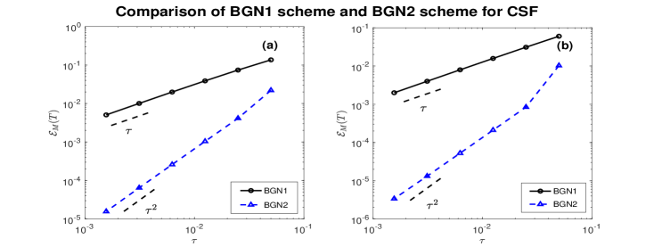
Figure 1: Log-log plot of the numerical errors at time $T=0.25$ measured by the manifold distance for BGN1 (2.3) and BGN2 (2.5) schemes for solving the CSF with two different initial curves: (a) Shape 1 and (b) Shape 2, respectively, where the number of nodes is fixed as $N=10000$.

We begin our test by calculating the convergence of the BGN2 scheme (2.5) for the CSF with either Shape 1 or Shape 2 as initial data. Fig. 1 presents a log-log plot of the numerical errors at time $T=0.25$, measured by the manifold distance. The errors for the Hausdorff distance, which are similar, are not included here for brevity. To ensure a fair comparison, we also include the numerical results of the BGN1 scheme (2.3) under the same computational parameters, with a fixed number of grid points $N=10000$. As clearly shown in Fig. 1, the numerical error of the BGN2 scheme reduces very rapidly with second-order accuracy in time, while the BGN1 scheme only achieves first-order convergence.

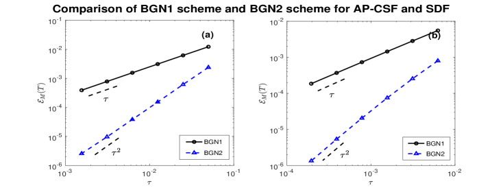
Figure 2: Log-log plot of the numerical errors at time $T=0.25$, measured by the manifold distance, for solving two different flows with Shape 2 as the initial curve: (a) AP-CSF and (b) SDF, respectively.

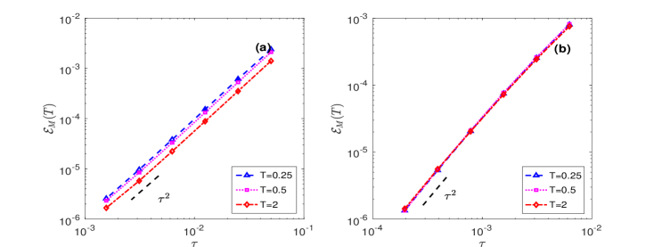
Figure 3: Log-log plot of the numerical errors measured by the manifold distance, at three different times (i.e., $T=0.25,0.5,2$) for solving two different flows with Shape 2 as the initial curve: (a) AP-CSF and (b) SDF, respectively.

Fig. 2 shows the temporal errors of the BGN2 scheme (4.3) for solving the AP-CSF and SDF with Shape 2 as initial data. It is clear that the numerical error of the BGN2 scheme converges quadratically, whereas the BGN1 scheme (4.2) converges only linearly. Moreover, since both the AP-CSF and SDF eventually evolve into a circle, we also investigate the convergence of the BGN2 scheme over long-time simulations. As illustrated in Fig. 3, the numerical errors at three different times $T=0.25,0.5,2$ of the BGN2 scheme all display quadratic convergence.

5.2 Comparison of computational costs

In order to show that the computational cost of the proposed BGN2 scheme is comparable to that of the BGN1 scheme, we present two examples about solving the CSF and SDF, respectively. The numerical codes were written by using MATLAB 2021b, and they were implemented in a MacBook Pro with 1.4GHz quad-core Intel Core i5 and 8GB RAM.

Table 4: Comparisons of the CPU times (seconds) and the numerical errors measured from the manifold distance $\mathcal{E}_{M}(T)$ and Hausdorff distance $\mathcal{E}_{H}(T)$ for the BGN2 scheme (2.5) and the BGN1 scheme (2.3) applied to CSF, where the initial shape is chosen as Shape 1, with $\tau=0.5/N$ and $T=0.05$.

BGN1 scheme (2.3)				BGN2 scheme (2.5)
$N$	$\mathcal{E}_{M}(T)$	$\mathcal{E}_{H}(T)$	Time	$N$	$\mathcal{E}_{M}(T)$	$\mathcal{E}_{H}(T)$	Time
320	5.61E-4	1.25E-4	0.350s	160	8.35E-4	2.02E-4	0.200s
640	3.34E-4	6.37E-5	1.70s	320	2.09E-4	5.04E-5	0.430s
1280	1.81E-4	3.22E-5	9.85s	640	5.20E-5	1.27E-5	2.30s
2560	9.38E-5	1.62E-5	110s	1280	1.29E-5	3.20E-6	12.9s
5120	4.78E-5	8.16E-5	1893s	2560	3.08E-6	8.16E-7	130s

Table 4 displays a comparison of CPU times in seconds and numerical errors at time $T=0.05$, as measured by the manifold distance $\mathcal{E}_{M}(T)$ and Hausdorff distance $\mathcal{E}_{H}(T)$, using the BGN2 scheme (2.5) and the BGN1 scheme (2.3) for solving the CSF, where the initial shape is chosen as Shape 1. Table 5 provides similar results for solving the SDF with Shape 3 as its initial shape. Based on the findings presented in Tables 4 and 5, the following conclusions can be drawn: (i) On the same mesh, the computational cost of the BGN2 scheme is slightly higher compared to the BGN1 scheme, as it involves additional calculations for the initial values and the right-hand side of the linear system at each time level. However, the numerical solution obtained using the BGN2 scheme is significantly more accurate than the BGN1 scheme. (ii) Achieving the same level of accuracy requires a much higher computational cost for the BGN1 scheme. For instance, as demonstrated in Table 4, when comparing the results of the BGN1 scheme with $N=5120$ and the BGN2 scheme with $N=1280$, it is evident that the BGN2 scheme is not only more accurate but also more than $100$ times faster than the BGN1 scheme. Similar trends can be observed in Table 5 for the SDF.

Table 5: Comparisons of the CPU times (seconds) and the numerical errors measured by the manifold distance $\mathcal{E}_{M}(T)$ and Hausdorff distance $\mathcal{E}_{H}(T)$ using the BGN2 scheme (4.6) and the BGN1 scheme (4.5) for SDF, where the initial shape is chosen as Shape 3, with $\tau=0.5/N$, and $T=0.05$.

BGN1 scheme (4.5)				BGN2 scheme (4.6)
$N$	$\mathcal{E}_{M}(T)$	$\mathcal{E}_{H}(T)$	Time	$N$	$\mathcal{E}_{M}(T)$	$\mathcal{E}_{H}(T)$	Time
320	4.73E-3	6.91E-4	0.470s	160	7.51E-3	2.62E-3	0.260s
640	2.24E-3	3.38E-4	2.03s	320	2.53E-3	1.14E-3	0.610s
1280	1.10E-3	1.67E-4	12.6s	640	8.28E-4	4.17E-4	2.270s
2560	5.53E-4	8.34E-5	132.6s	1280	2.30E-4	1.12E-4	15.1s
5120	2.80E-4	4.16E-5	2180s	2560	5.42E-5	2.82E-5	153s

5.3 Applications to the curve evolution

As is well-known, the AP-CSF and SDF possess some structure-preserving properties, such as the perimeter decreasing and area conserving properties [23, 24, 7]. In this subsection, we investigate the structure-preserving properties of the proposed BGN2 schemes (4.3) and (4.6) applied to AP-CSF and SDF, respectively. As an example, we mainly focus on the SDF here. Moreover, we will discuss the importance of the mesh regularization procedure.

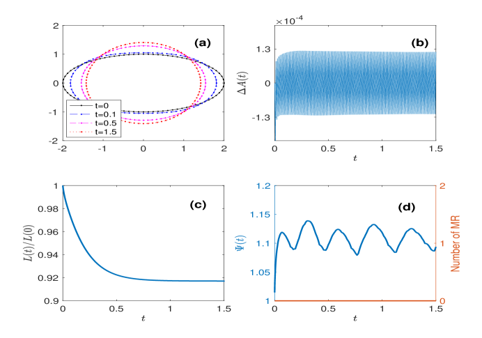
Figure 4: (a) Several snapshots of the curve evolution controlled by the SDF, starting with Shape 2 as its initial shape. (b) The normalized area loss as a function of time. (c) The normalized perimeter as a function of time. (d) The mesh ratio function $\Psi(t)$ (in blue line) and the number of mesh regularizations (in red line). For (a)-(b), we used $N=80$ and $\tau=1/160$ while for (c)-(d), $N=640$ and $\tau=1/1280$.

Fig. 4 (a) illustrates the evolution of an initially elliptic curve, referred to as Shape 2, driven by SDF towards its equilibrium state. Fig. 4(b)-(d) show the evolution of various geometric quantities during the process: the relative area loss $\Delta A(t)$, the normalized perimeter $L(t)/L(0)$, and the mesh distribution function $\Psi(t)$, which are defined respectively as

$$\Delta A(t)|_{t=t_{m}}=\frac{A^{m}-A^{0}}{A^{0}},\quad\left.\frac{L(t)}{L(0)}\right|_{t=t_{m}}=\frac{L^{m}}{L^{0}},\quad\Psi(t)|_{t=t_{m}}=\Psi^{m},\quad m\geq 0,$$

where $A^{m}$ is the area enclosed by the polygon determined by $\mathbf{X}^{m}$, $L^{m}$ represents the perimeter of the polygon, and the mesh ratio $\Psi^{m}$ is defined in (2.7). As depicted in Fig. 4(b), the area loss exhibits a weakly oscillating behavior, which may result from the two-step structure of the BGN2 scheme. It is worth noting that despite the oscillations, the normalized area loss remains very low, consistently below $0.01\%$. By employing a smaller grid size, the area loss can be further reduced, and it is significantly lower than that of the BGN1 scheme under the same computational parameters. Furthermore, Fig. 4(c) shows the BGN2 scheme preserves the perimeter-decreasing property of the SDF numerically. Furthermore, in Fig. 4(d), it can be observed that the mesh distribution function $\Psi(t)$ remains lower than $1.2$ during the evolution. This indicates that the mesh distribution remains well-maintained and almost equidistributed during the process. Therefore, in this scenario, there is no need to perform the mesh regularization procedure because $\Psi(t)$ is always smaller than the chosen threshold $n_{\text{MR}}$ (here we choose it as $10$) in the simulations.

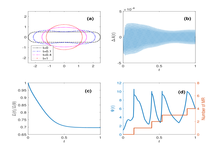
Figure 5: (a) Several snapshots of the curve evolution controlled by the SDF, starting with Shape 3 as its initial shape. (b) The normalized area loss as a function of time. (c) The normalized perimeter as a function of time. (d) The mesh distribution function $\Psi(t)$ (in blue line) and the number of mesh regularizations (in red line). For (a)-(b) we used $N=80$ and $\tau=1/160$ while $N=640$ and $\tau=1/1280$ for (c)-(d).

To provide a more comprehensive comparison, we conduct simulations of evolution of Shape 3 curve driven by the SDF. Fig. 5(b)-(c) demonstrates that the BGN2 scheme effectively preserves two crucial geometric properties of the SDF: the conservation of area and the reduction of perimeter properties [23, 7]. It should be noted that Fig. 5(d) reveals that without the implementation of mesh regularization, the mesh distribution function $\Psi(t)$ can become very large. Therefore, in our algorithm, when $\Psi(t)$ exceeds a threshold $n_{\text{MR}}$, we employ the BGN1 scheme (4.5) for a single run to perform mesh regularization, similar to Step 3 of Algorithm 2.2. As clearly shown in Fig. 5(d), following this step, the mesh ratio rapidly decreases to a low value, which makes the method more stable. Importantly, this mesh regularization procedure is only required four times throughout the entire evolution, without sacrificing the accuracy of the BGN2 scheme (cf. Table 5).

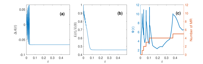
Figure 6: Evolution of the three geometrical quantities when the initial data is prepared as in Algorithm 2.1: (a) the normalized area loss, (b) the normalied perimeter, (c) the mesh distribution function $\Psi(t)$, with mesh regularization procedure.

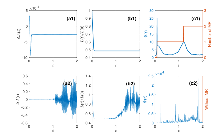
Figure 7: Evolution of the three geometrical quantities when the initial data is prepared as in Remark 2.2: (a) the normalized area loss, (b) the normalized perimeter, (c) the mesh distribution function $\Psi(t)$, with mesh regularization procedure (shown in the top row) and without mesh regularization procedure (shown in the bottom row).

Next, we proceed to simulate the evolution of a nonconvex curve, referred to as Shape 4. Fig. 6 and Fig. 7 (top row) show the evolution of the geometric quantities based on two different initial data preparations: Algorithm 2.1 and Remark 2.2, respectively. A comparison of the results reveals the superiority of the latter approach for several reasons: (i) the magnitude of area loss is significantly lower when using the approach in Remark 2.2; (ii) the perimeter-decreasing property is preserved while the perimeter oscillates at the beginning when using Algorithm 2.1; (iii) the number of mesh regularization implementations is smaller with the approach in Remark 2.2. Thus we recommend preparing the data for a nonconvex initial curve following the approach outlined in Remark 2.2. Fig. 7 (bottom row) illustrates the evolution of the same quantities without implementation of mesh regularization. In this case, all three quantities exhibit significant oscillations after a certain time period, and the area loss and mesh ratio of the polygon becomes excessively large, resulting in the breakdown of the BGN2 scheme. Notably, mesh clustering has happened at $t=1$ (see Fig. 8 (c2)), eventually leading to mesh distortion at $t=2$ (see Fig. 8 (d2)). These issues can be avoided by implementing mesh regularization (see 7 (a1)-(c1) and Fig. 8 (a1)-(d1)). This demonstrates the essential role of mesh regularization in the effectiveness of the BGN2 scheme and the BGN1 scheme can greatly improve the mesh distribution.

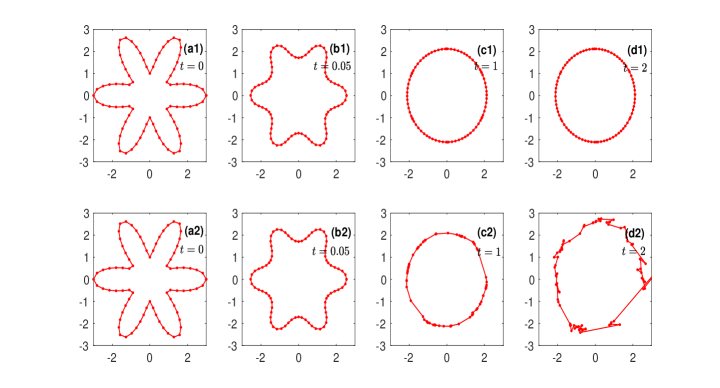
Figure 8: Evolution of the curve driven by SDF starting with Shape 4 as initial data by using the BGN2 scheme (4.6) with mesh regularization procedure (shown in the top row), and without mesh regularization procedure (shown in the bottom row). The simulations are conducted with a grid number of $N=80$ and a time step size $\tau=1/160$.

We close this section by simulating the evolution of a nonconvex initial curve [30, 3, 28] driven by CSF, AP-CSF and SDF using the BGN2 schemes. The initial curve can be parametrized as

$$\mathbf{X}_{0}(\rho)=(\cos(2\pi\rho),\sin(\cos(2\pi\rho))+\sin(2\pi\rho)(0.7+\sin(2\pi\rho)\sin^{2}(6\pi\rho))),$$

for $\rho\in\mathbb{I}=[0,1]$. The numerical results are depicted in Fig. 9. As shown in this figure, the CSF initially transforms the intricate curve into a circle before it disappear. Both the AP-CSF and SDF drive the curve to evolve into a perfect circle as its equilibrium shape.

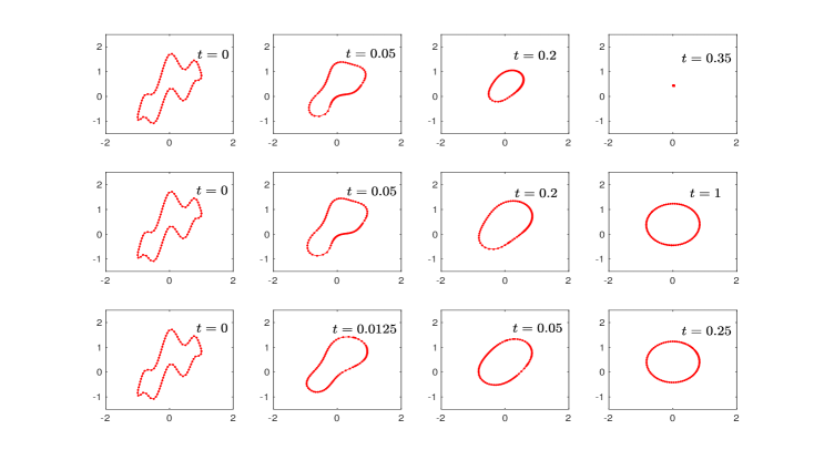
Figure 9: Snapshots of the curve evolution using the proposed BGN2 schemes for three distinct geometric flows: CSF (first row), AP-CSF (second row) and SDF (third row). The simulations are conducted with $N=80$ and $\tau=1/640$.

6 Conclusions

We proposed a novel temporal second-order, BGN-based parametric finite element method (BGN2 scheme) for solving geometric flows of curves such as CSF, AP-CSF and SDF. Based on the BGN formulation and the corresponding semi-discrete FEM approximation [10, 11, 14], our numerical method employs a Crank-Nicolson leap-frog method to discretize in time and the key innovation lies in choosing a discrete inner product over the curve $\Gamma^{m}$, such that the time level $t_{m}$ coincides with when all quantities have approximations with an error of $\mathcal{O}(\tau^{2})$. We established the well-posedness and mild energy stability of the fully-discrete scheme, subject to suitable assumptions. We emphasized the use of shape metrics (manifold distance and Hausdorff distance) rather than function norms (e.g., $L^{2}$-norm, $L^{\infty}$-norm) to measure the numerical errors of the BGN-based schemes. In the case of certain initial curves, such as a ‘flower’ shape, we found that the BGN2 scheme, in conjunction with the BGN1 scheme for mesh regularization, exhibited remarkable efficiency and stability in practical simulations. Extensive numerical experiments demonstrated that the proposed BGN2 scheme achieves second-order accuracy in time, as measured by the shape metrics, outperforming the BGN1 scheme in terms of accuracy.

Furthermore, it is worth mentioning that the approach we have presented for constructing a temporal high-order BGN-based scheme can be readily extended to address various other problems, such as anisotropic geometric flows [5], Willmore flow [13], two-phase flow [21], solid-state dewetting [32] and geometric flows in 3D [31].

In our future research, we will further investigate the development of structure-preserving temporal high-order BGN-based schemes [7, 23] and conduct the numerical analysis of the BGN-based schemes with respect to the shape metric. These investigations will contribute to enhancing the overall understanding and applicability of the BGN type scheme in different contexts.

CRediT authorship contribution statement

Wei Jiang: Conceptualization, Methodology, Supervision, Writing. Chunmei Su: Conceptualization, Methodology, Supervision, Writing. Ganghui Zhang: Methodology, Numerical experiments, Visualization and Writing.

Declaration of competing interest

The authors declare that they have no known competing financial interests or personal relationships that could have appeared to influence the work reported in this paper.

Data availability

No data was used for the research described in the article.

References

References

- [1] G. Aubert, P. Kornprobst, Mathematical problems in image processing, Vol. 147 of Applied Mathematical Science (2006), Springer.
- [2] Y. Bai, J. Yong, C. Liu, X. Liu, Y. Meng, Polyline approach for approximating Hausdorff distance between planar free-form curves, Computer-Aided Design 43 (2011) 687–698.
- [3] M. Balaz̆ovjech, K. Mikula, A higher order scheme for a tangentially stabilized plane curve shortening flow with a driving force, SIAM J. Sci. Comput. 33 (2011) 2277–2294.
- [4] W. Bao, H. Garcke, R. Nürnberg, Q. Zhao, Volume-preserving parametric finite element methods for axisymmetric geometric evolution equations, J. Comput. Phys. 460 (2022) article 111180.
- [5] W. Bao, W. Jiang, Y. Li, A symmetrized parametric finite element method for anisotropic surface diffusion of closed curves, SIAM J. Numer. Anal. 61 (2023) 617–641.
- [6] W. Bao, W. Jiang, Y. Wang, Q. Zhao, A parametric finite element method for solid-state dewetting problem with anisotropic surface energies, J. Comput. Phys. 330 (2017) 380–400.
- [7] W. Bao, Q. Zhao, A structure-preserving parametric finite element method for surface diffusion, SIAM J. Numer. Anal. 59 (2021) 2775–2799.
- [8] J. W. Barrett, K. Deckelnick, R. Nürnberg, A finite element error analysis for axisymmetric mean curvature flow, IMA J. Numer. Anal. 41 (2021) 1641–1667.
- [9] J. W. Barrett, K. Deckelnick, V. Styles, Numerical analysis for a system coupling curve evolution to reaction diffusion on the curve, SIAM J. Numer. Anal. 55 (2017) 1080–1100.
- [10] J. W. Barrett, H. Garcke, R. Nürnberg, A parametric finite element method for fourth order geometric evolution equations, J. Comput. Phys. 222 (2007) 441–467.
- [11] J. W. Barrett, H. Garcke, R. Nürnberg, On the variational approximation of combined second and fourth order geometric evolution equations, SIAM J. Sci. Comput. 29 (2007) 1006–1041.
- [12] J. W. Barrett, H. Garcke, R. Nürnberg, On the parametric finite element approximation of evolving hypersurfaces in , J. Comput. Phys. 227 (2008) 4281–4307.
- [13] J. W. Barrett, H. Garcke and R. Nürnberg, Parametric approximation of Willmore flow and related geometric evolution equations, SIAM J. Sci. Comput. 31 (2008) 225–253.
- [14] J. W. Barrett, H. Garcke, R. Nürnberg, Parametric finite element method approximations of curvature driven interface evolutions, Handb. Numer. Anal. 21, Elsevier, Amsterdam, (2020), pp. 275–423.
- [15] E. Bänsch, P. Morin, R.H. Nochetto, A finite element method for surface diffusion: the parametric case, J. Comput. Phys. 203 (2005) 321–343.
- [16] K. Deckelnick, G. Dziuk, On the approximation of the curve shortening flow, in Calculus of Variations, Applications and Computations (Pont-à-Mousson, 1994), Pitman Res. Notes Math. Ser. 326, Longman Sci. Tech., Harlow, UK, 1995, pp. 100–108.
- [17] K. Deckelnick, G. Dziuk, C. M. Elliott, Computation of geometric partial differential equations and mean curvature flow, Acta Numer. 14 (2005) 139–232.
- [18] G. Dziuk, Convergence of a semi-discrete scheme for the curve shortening flow, Math. Models Methods Appl. Sci. 04 (1994) 589–606.
- [19] G. Dziuk, Discrete anisotropic curve shortening flow, SIAM J. Numer. Anal. 36 (1999) 1808–1830.
- [20] C. M. Elliott, H. Fritz, On approximations of the curve shortening flow and of the mean curvature flow based on the DeTurck trick, IMA J. Numer. Anal. 37 (2016) 543–603.
- [21] G. Garcke, R. Nürnberg, Q. Zhao, Structure-preserving discretizations of two-phase Navier–Stokes flow using fitted and unfitted approaches, J. Comput. Phys. 489 (2023) article 112276.
- [22] N. Hurl, W. Layton, Y. Li, M. Moraiti, The unstable mode in the Crank-Nicolson Leap-Frog method is stable, Int. J. Numer. Anal. Model. 13 (2016) 753-762.
- [23] W. Jiang, B. Li, A perimeter-decreasing and area-conserving algorithm for surface diffusion flow of curves, J. Comput. Phys. 443 (2021) article 110531.
- [24] W. Jiang, C. Su, G. Zhang, A convexity-preserving and perimeter-decreasing parametric finite element method for the area-preserving curve shortening flow, SIAM J. Numer. Anal. 61 (2023) 1989–2010.
- [25] M. Kimura, Numerical analysis of moving boundary problems using the boundary tracking method, Japan J. Indust. Appl. Math. 14 (1997) 373-398.
- [26] B. Kovács, B. Li, C. Lubich, A convergent evolving finite element algorithm for mean curvature flow of closed surfaces, Numer. Math. 143 (2019) 797–853.
- [27] B. Kovács, B. Li, C. Lubich, A convergent algorithm for forced mean curvature flow driven by diffusion on the surface, Interfaces Free Bound. 22 (2020) 443–464.
- [28] J. A. Mackenzie, M. Nolan, C. F. Rowlatt, R. H. Insall, An adaptive moving mesh method for forced curve shortening flow, SIAM J. Sci. Comput. 41 (2019) A1170–A1200.
- [29] K. Mikula, D. Sevcovic, Evolution of plane curves driven by a nonlinear function of curvature and anisotropy, SIAM J. Appl. Math. 61 (2001) 1473–1501.
- [30] K. Mikula, D. Sevcovic, A direct method for solving an anisotropic mean curvature flow of plane curves with an external force, Math. Methods Appl. Sci. 27 (2004) 1545–1565.
- [31] Q. Zhao, W. Jiang, W. Bao, A parametric finite element method for solid-state dewetting problems in three dimensions, SIAM J. Sci. Comput. 42 (2020) B327–B352.
- [32] Q. Zhao, W. Jiang, W. Bao, An energy-stable parametric finite element method for simulating solid-state dewetting, IMA J. Numer. Anal. 41 (2021) 2026–2055.