Deep regression learning with optimal loss function

Abstract

Due to powerful function fitting ability and effective training algorithms of neural networks, in this paper, we develop a novel efficient and robust nonparametric regression estimator under a framework of feedforward neural network (FNN). There are several interesting characteristics for the proposed estimator. First, the loss function is built upon an estimated maximum likelihood function, who integrates the information from observed data, as well as the information from data structure. Consequently, the resulting estimator has desirable optimal properties, such as efficiency. Second, different from the traditional maximum likelihood estimation (MLE), we do not require the specification of the distribution, hence the proposed estimator is flexible to any kind of distribution, such as heavy tails, multimodal or heterogeneous distribution. Third, the proposed loss function relies on probabilities rather than direct observations as in least square loss, hence contributes the robustness in the proposed estimator. Finally, the proposed loss function involves nonparametric regression function only. This enables the direct application of the existing packages, and thus the computation and programming are simple. We establish the large sample property of the proposed estimator in terms of its excess risk and minimax near-optimal rate. The theoretical results demonstrate that the proposed estimator is equivalent to the true MLE in which the density function is known. Our simulation studies show that the proposed estimator outperforms the existing methods in terms of prediction accuracy, efficiency and robustness. Particularly, it is comparable to the true MLE, and even gets better as the sample size increases. This implies that the adaptive and data-driven loss function from the estimated density may offer an additional avenue for capturing valuable information. We further apply the proposed method to four real data examples, resulting in significantly reduced out-of-sample prediction errors compared to existing methods.

Keywords: Estimated maximum likelihood estimation, feedforward neural network, excess risk, kernel density estimation.

1 Introduction

Consider a nonparametric regression model,

$$Y = g(\bm{X})+\epsilon,$$ (1)

where $Y\in\mathbb{R}$ is a response variable, $\bm{X}\in\mathcal{X}\subseteqq\mathbb{R}^{d}$ is a $d$-dimensional vector of predictors, $g:\mathcal{X}\rightarrow\mathbb{R}$ is an unknown regression function, $\epsilon$ is an error independent of $\bm{X}$. Nonparametric regression is a basic and core problem in statistics and machine learning, where the purpose is estimating the unknown target regression function $g$ given independent and identically distributed (i.i.d.) samples $S\equiv{(\bm{X}_{i},Y_{i})}_{i=1}^{n}$ with the sample size $n$. Since the distribution of $\epsilon$ is unknown, $g(\cdot)$ is usually estimated based on the least square (LS) criterion, that is,

$$\hat{g}=\underset{g:\mathbb{R}^{d}\rightarrow\mathbb{R}}{\arg\min}\frac{1}{n}\sum_{i=1}^{n}\left\{Y_{i}-g(\bm{X}_{i})\right\}^{2}.$$ (2)

Driven by various nonparametric approximation techniques, there is a vast literature on nonparametric regression. For example, tree regression (Breiman, 2017), random forests (Breiman, 2001), and nonparametric smoothing methods such as nearest neighbor regression (Cheng, 1984; Devroye et al., 1994), kernel regression (Nadaraya, 1964; Watson, 1964; Hall and Huang, 2001), local polynomial regression (Fan and Gijbels, 2018), spline approximation (Schumaker, 2007) and reproducing kernel regression (Berlinet and Thomas-Agnan, 2011; Lv et al., 2018), among others.

Recently, attributed to powerful function fitting ability, well-designed neural network architectures and effective training algorithms and high-performance computing technologies, deep neural network (DNN) with the empirical LS loss function has enjoyed tremendous success in a variety of applications, such as the fields of computer vision, natural language processing, speech recognition, among others. Based on the theoretical results concerning approximation error and stochastic error, with the LS loss, several inspiring works have obtained the minimax near-optimal rate at $n^{-\frac{2\beta}{2\beta+d}}(\log n)^{s}$ for learning the regression function $g$ under feedforward neural network (FNN), with the assumption that $g$ is $\beta$-H$\ddot{o}$lder smooth. In these works, the response variable or the error term is assumed to be bounded (Györfi et al., 2002; Farrell et al., 2021), have finite $p$-th moment with $p>1$ (Kohler and Langer, 2021; Kohler et al., 2022), sub-Gaussian (Bauer and Kohler, 2019; Chen et al., 2019; Schmidt-Hieber, 2019; 2020; Fan and Gu, 2022; Bhattacharya et al., 2023), sub-exponential (Jiao et al., 2021; Yan and Yao, 2023) or have finite variance (Liu et al., 2022).

The LS criterion based estimators are mathematically convenient, easily implemented, and efficient when the error $\epsilon$ is normally distributed. However, as it is expressed in (2), the LS loss is sensitive to large errors, that is, the LS estimator is severely influenced by outliers, resulting in unstable and unreliable estimation. In the era of “big data”, data generation mechanism and collection are unmanageable, and thus non-Gaussian noises or outliers are almost inevitable. To address the unstableness, a lot of robust methods based on traditional nonparametric regression techniques have been developed, for example, the kernel M-smoother (Härdle, 1989), median smoothing(Tukey et al., 1977) , locally weighted regression (Stone, 1977; Cleveland, 1979), the local least absolute method (Wang and Scott, 1994), quantile regression (Koenker and Bassett Jr, 1978; He et al., 2013; Lv et al., 2018), among others.

Recently, within the framework of FNN, several robust methods have been introduced to address non-Gaussian noise problems, and corresponding convergence rates for learning the function $g$ have also been established. For instance, Lederer, (2020); Shen et al., 2021b and Fan et al., (2022) have explored non-asymptotic error bounds of the estimators that minimizing robust loss functions, such as the least-absolute deviation loss (Bassett Jr and Koenker, 1978), Huber loss (Huber, 1973), Cauchy loss and Tukey’s biweight loss (Beaton and Tukey, 1974). Particularly, based on a general robust loss function satisfying a Lipschitz continuity, Farrell et al., (2021) have demonstrated the convergence rate $n^{-\frac{2\beta}{2\beta+d}}(\log n)^{4}$ with the assumption that the response is bounded, which means that heavy-tail error is not applicable. To relax the bounded restriction on the response, Shen et al., 2021b and Shen et al., 2021a have established the convergence rate $n^{-\frac{2\beta}{2\beta+d}+1/p}(\log n)^{c}$ under the assumption that the $p$-th moment of response is bounded for some $p>1$. These methods are proposed for improving the robustness, they are sub-optimal in terms of efficiency.

This work attempts to provide a loss function which is efficient as well as robust for nonparametric regression estimation within the framework of FNN. It is worth noting that in the least squares (LS) criterion, observations in which the response variable $Y_{i}$ deviates significantly from the conditional mean $g(\bm{X}_{i})$ play a significant role, which may seem counterintuitive. In fact, when estimating the conditional mean $g(\cdot)$, observations in which $Y_{i}$ is closer to $g(\bm{X}_{i})$ are supposed to logically carry more information than those where the response is away from the conditional mean. This can be expressed in terms of probability of observation. Therefore, we propose a loss function based on the estimated likelihood function, which has the form of

$$\hat{g}=\underset{g:\mathbb{R}^{d}\rightarrow\mathbb{R}}{\arg\max}\frac{1}{n}\sum_{i=1}^{n}\log\hat{f}(Y_{i}-g(\bm{X}_{i})),$$ (3)

where $\hat{f}$ is an estimator of the density function of $\epsilon_{i}=Y_{i}-g(\bm{X}_{i})$. We simplify the FNN estimators of $g(\cdot)$ based on maximizing Estimated log-Likelihood functions (3) by EML-FNN, which is expected to have the desirable optimal properties since we use the density function and leverage the data distribution. In addition, different from the traditional maximum likelihood estimator (MLE) where $f(\cdot)$ is known, the proposed EML-FNN is flexible as it avoids specifying the error distribution. Moreover, the quasi-likelihood loss (3), which relies on probabilities rather than direct observations as in LSE, contributes the robustness of the proposed EML-FNN. More interesting, in comparison to the MLE where $f(\cdot)$ is known, the adaptive form via estimating the density $f(\cdot)$ in (3) proves to be effective in learning the data structure and offers an additional avenue for capturing information. This is supported by our simulation studies. Specifically, Figures 1 to 3 reveal the following results: when $\varepsilon_{i}$ follows a normal distribution where the LSE is equivalent to the MLE, the EML-FNN performs slightly better than FNN estimators based on Least Square Error (LSE-FNN) for data with a larger sample size ($n=1024$). However, when $\varepsilon_{i}$ deviates from a normal distribution or has heterogeneous variances, the EML-FNN significantly outperforms the LSE-FNN. The enhanced performance may be attributed to the utilization of structural information via the estimated density function $\hat{f}(\cdot)$.

With the explicit form of Nadaraya–Watson kernel estimator for the density function of $\epsilon_{i}$, we develop a FNN estimation for $g$ that circumvents estimating the unknown density function, resulting in an objective function that solely involves $g$. This enables the direct application of existing packages Pytorch (Paszke et al., 2019) and Scikit-learn (Pedregosa et al., 2011) in python, simplifying the computation and programming. We establish the large sample property of $\hat{g}$ in terms of its excess risk and the minimax rate, which demonstrate that the proposed estimator for $g$ is equivalent to the one based on (3) when the density function is known. As a result, the proposed deep learning approach for $g$ exhibits the desired optimal properties, such as efficiency (Zhou et al., 2018; 2019). Finally, we employ the proposed method to analyze four real datasets. Table 1 shows that the proposed EML-FNN provides much higher prediction accuracy than the existing methods for each dataset.

The paper is structured as follows. In Section 2, we introduce the proposed EML-FNN. In Section 3, we establish the large sample property of $\hat{g}$ in terms of its excess risk and the minimax rate. Section 4 provides simulation studies to investigate the performance of the proposed method via the comparison with the competing estimation methods. In Section 5, we apply the proposed method to analyze four real data. We conclude the paper with a discussion in Section 6. Technical proofs are included in the Supplementary Material.

2 Method

We estimate $g$ under the framework of FNN. In particular, we set $\mathcal{G}$ to be a function class consisting of ReLU neural networks, that is, $\mathcal{G}:=\mathcal{G}_{\mathcal{D},\mathcal{U},\mathcal{W},\mathcal{S},\mathcal{B}},$ where the input data is the predictor $X$, forming the first layer, and the output is the last layer of the network; Such a network $\mathcal{G}$ has $\mathcal{D}$ hidden layers and a total of $(\mathcal{D}+2)$ layers. Denote the width of layer $j$ by $d_{j}$, $j=0,\cdots,\mathcal{D},\mathcal{D}+1$ with $d_{0}=d$ representing the dimension of the input $X$, and $d_{\mathcal{D}+1}=1$ representing the dimension of the response $Y$. The width $\mathcal{W}$ is defined as the maximum width among the hidden layers, i.e., $\mathcal{W}=\max{(d_{1},...,d_{\mathcal{D}})}$. The size $\mathcal{S}$ is defined as the total number of parameters in the network $\mathcal{G}$, given by $\mathcal{S}=\sum_{i=0}^{\mathcal{D}}d_{i+1}\times(d_{i}+1)$; The number of neurons $\mathcal{U}$ is defined as the total number of computational units in the hidden layers, given by $\mathcal{U}=\sum_{i=1}^{\mathcal{D}}d_{i}$. Further, we assume every function $g\in\mathcal{G}$ satisfies $|g|_{\infty}\leq\mathcal{B}$ with $\mathcal{B}$ being a positive constant.

With $g\in\mathcal{G}$, $g$ can be estimated by

$$\arg\min_{g\in\mathcal{G}}\left\{\frac{1}{n}\sum_{i=1}^{n}\rho(Y_{i}-g(\bm{X}_{i}))\right\},$$ (4)

where $\rho(\cdot)$ is a given loss function, for example, the least squares $\rho(t)=t^{2}$; least absolute criteria $\rho(t)=|t|$; Huber loss, Cauchy loss, and Tukey’s biweight loss, and so on. The LS based estimator is efficient only when the error $\epsilon$ is normally distributed. The estimators based on robust loss functions such as least absolute, Huber, Cauchy and Tukey’s biweight are robust but they are sub-optimal in terms of efficiency.

When $f(\cdot)$ is known, an ideal estimator of $g$ can be obtained by,

$$\hat{g}=\arg\min_{g\in\mathcal{G}}\mathcal{R}_{n}(g):=\arg\min_{g\in\mathcal{G}}\left\{\frac{1}{n}\sum_{i=1}^{n}\left(-\log f(Y_{i}-g(\bm{X}_{i}))\right)\right\}.$$ (5)

However, in reality, $f$ is usually unknown. To ensure that we do not misspecify the distribution and simultaneously obtain an estimator based on optimal loss, we employ kernel techniques to estimate the density function $f$. That is,

$$\hat{f}(z)=\frac{1}{n}\sum_{i=1}^{n}\mathcal{K}_{h}(\epsilon_{i},z),$$ (6)

where $\mathcal{K}_{h}(y_{1},y_{2})=K(\frac{y_{1}-y_{2}}{h})/h$, $h$ is a bandwidth and $K(\cdot)$ is a kernel function.

Replacing $f(\cdot)$ in (5) with $\hat{f}$, we estimate $g$ by,

$$\hat{g}=\arg\min_{g\in\mathcal{G}}\hat{\mathcal{R}}_{n}(g)=\arg\min_{g\in\mathcal{G}}n^{-1}\sum_{i=1}^{n}\left(-\log\hat{f}(Y_{i}-g(\bm{X}_{i}))\right).$$ (7)

That is,

$$\hat{g}=\arg\min_{g\in\mathcal{G}}\hat{\mathcal{R}}_{n}(g)=\arg\min_{g\in\mathcal{G}}n^{-1}\sum_{i=1}^{n}\left(-\log\frac{1}{n}\sum_{j=1}^{n}\mathcal{K}_{h}(Y_{j}-g(\bm{X}_{j}),Y_{i}-g(\bm{X}_{i}))\right).$$ (8)

Recall that the conventional FNN (Chen et al., 2019; Nakada and Imaizumi, 2019; Schmidt-Hieber, 2020; Kohler and Langer, 2021; Jiao et al., 2021; Kohler et al., 2022; Liu et al., 2022; Fan and Gu, 2022; Yan and Yao, 2023; Bhattacharya et al., 2023) minimizes a least square objective and is sensitive to the data’s distribution type and outliers, which leading to the development of the robust FNN (Lederer, 2020; Shen et al., 2021b ; Fan et al., 2022). However, the enhanced robustness comes at the cost of efficiency. In contrast to existing methods, our approach stands out by utilizing a MLE criterion as the objective function, thereby achieving both efficiency and robustness. In particular, efficiency is attained by fully leveraging the data distribution, robustness is added to our estimator because our proposed loss function relies on probabilities rather than direct observations as in LS. Moreover, the kernel-based estimation approach benefits from the smooth continuity of kernel functions, facilitating gradient calculations and overcoming non-differentiability issues when dealing with densities such as the uniform distribution, mixture distribution, and heteroscedasticity. Finally, the proposed loss function (8) involves $g$ only. This enables the direct application of packages Pytorch (Paszke et al., 2019) and Scikit-learn (Pedregosa et al., 2011) in python, simplifying the computation and programming.

The proposed $\hat{\mathcal{R}}_{n}(g)$ involves a tuning parameter $h$. According to the property of kernel approximation, a smaller $h$ yields a more accurate density approximation but with a larger variance. Fortunately, the summation over individuals mitigates the increased variance caused by a small $h$. Therefore, when computational feasibility allows, a smaller value of $h$ is preferred. The conclusion is supported by both our theoretical and numerical results. In practice, we use the Gaussian kernel function and set $\hat{f}=1e-5$ when $\hat{f}<1e-5$ because logarithmic transformation is required in the objective function.

3 Large sample properties

In this section, we establish the large sample property of $\hat{g}$ in terms of its excess risk, which is defined as the difference between the risks of ${g}$ and $g^{*}$:

$$\mathcal{R}(g)-\mathcal{R}(g^{*})=\mathbb{E}\left(-\log f(Y_{i}-g(\bm{X}_{i}))\right)-\mathbb{E}\left(-\log f(Y_{i}-g^{*}(\bm{X}_{i}))\right),$$

where $g^{*}$ is defined as

$$g^{*}:=\arg\min_{g}\mathcal{R}(g)=\arg\min_{g}\mathbb{E}\left(-\log f\left(Y_{i}-g(\bm{X}_{i})\right)\right).$$

The minimizer is taken over the entire space, and thus implies that $g^{*}$ does not necessarily belong to the set $\mathcal{G}$. We further define $g_{\mathcal{G}}^{*}:=\arg\min_{g\in\mathcal{G}}\mathcal{R}(g)$ in the set $\mathcal{G}$.

Denote $f^{(r)}(\cdot)$ to be the $r$th derivative of $f$, and $f_{\bm{x}}(\cdot)$ to be the density function of covariates $\bm{X}$, who is supported on a bounded set, and for simplicity, we assume this bounded set to be $[0,1]^{d}$. In the rest of the paper, the symbol $c$ denotes a positive constant which may vary across different contexts. The following conditions are required for establishing the rate of the excess risk:

1. Kernel: Let $U_{r}=\int K(t)t^{r}dt$ and $v_{r}=\int K^{2}(t)t^{r}dt$. Assume the kernel function $K(\cdot)$ has a bounded second derivative, $U_{0}=1$ and $U_{1}=0$.

2. Bandwidth: $h\to 0$ and $nh\to\infty$ as $n\rightarrow\infty$.

3. Density function $f$: Assume the density function $f(\cdot)$ has a continuous second derivative and satisfies $f(\epsilon)>c>0$ for any $\epsilon$ belonging to the support set of $f$.

4. Function class for $g$ and $g^{*}$: For any function $g\in\mathcal{G}$ and the true function $g^{*}$, we assume $\|g\|_{\infty}<\mathcal{B}$ and $\|g^{*}\|_{\infty}<\mathcal{B}$.

Condition (C1) is a mild condition for the kernel function, which is easy to be satisfied when the kernel function is a symmetric density function. Condition (C2) is the most commonly used assumption for the bandwidth. Condition (C3) requires a lower bound of the density function to avoid tail-related problems. The simulation studies, where the lower bounded condition is not met across all four distributions, demonstrate that the proposed estimator maintains its effectiveness even in scenarios where the condition does not hold. Condition (C4) is a bounded condition for the function class $\mathcal{G}$ and the true function $g^{*}$, which is commonly used in Shen et al., (2019); Lu et al., (2021); Chen et al., (2019); Yarotsky, (2017). It is noteworthy that, in cases where the explicit depiction of the approximation error for the function class $\mathcal{G}$ to $g^{*}$ becomes necessary, an additional condition will be introduced concerning the category to which $g^{*}$ belongs. This is demonstrated in Corollary 1.

Define $\mathcal{G}|_{\bm{x}}:=\{g(\bm{x}_{1}),g(\bm{x}_{2}),\cdots,g(\bm{x}_{n}):g\in\mathcal{G}\}$ for a given sequence $\bm{x}=(\bm{x}_{1},\cdots,\bm{x}_{n})$ and denote $\mathcal{N}_{2n}(\delta,\|\cdot\|_{\infty},\mathcal{G}|_{\bm{x}})$ to be the covering number of $\mathcal{G}|_{\bm{x}}$ under the norm $\|\cdot\|_{\infty}$ with radius $\delta$. Let $A\preceq B$ represent $A\leq cB$ for a postive constant $c$. In the following Theorems 1 and 2, we show the excess risk of the proposed estimator under the true density function and the estimated density function to see how much difference of the proposed estimator from the true MLE estimator, which is defined as

$$\hat{g}_{oracle}=\arg\min_{g\in\mathcal{G}}\left\{\frac{1}{n}\sum_{i=1}^{n}\big{(}-\log f(Y_{i}-g(\bm{X}_{i}))\big{)}\right\}.$$ (9)

Theorem 1.

Under Conditions (C3) and (C4), we have that, as $n\rightarrow\infty$,

$$\mathbb{E}\left(\mathcal{R}(\hat{g}_{oracle})-\mathcal{R}(g^{*})\right)\preceq\frac{\log\mathcal{N}_{2n}(n^{-1},\|\cdot\|_{\infty},\mathcal{G}|_{\bm{x}})}{n}+\big{(}\mathcal{R}(g^{*}_{\mathcal{G}})-\mathcal{R}(g^{*})\big{)}.$$

Recall that the excess risk of the LS estimator, takes the form: $\frac{\mathcal{B}^{2}\log 2\mathcal{N}_{2n}(n^{-1},|\cdot|_{\infty},\mathcal{G}|_{\bm{x}})(\log n)^{c}}{n}+\left(\mathcal{R}(g^{*}_{\mathcal{G}})-\mathcal{R}(g^{*})\right)$ for some positive constant $c$ with the condition of bounded response (Györfi et al., 2002; Farrell et al., 2021) or bounded $p$-th moment (Kohler and Langer, 2021; Kohler et al., 2022). For the robust loss considered in Shen et al., 2021b , the excess risk has the form of: $\frac{\lambda_{L}\mathcal{B}\log 2\mathcal{N}_{2n}(n^{-1},|\cdot|_{\infty},\mathcal{G}|_{\bm{x}})(\log n)^{c}}{n^{1-1/p}}+\left(\mathcal{R}(g^{*}_{\mathcal{G}})-\mathcal{R}(g^{*})\right)$, where $p$ represents the bounded $p$-th moment of the outcome, and $\lambda_{L}$ represents the Lipschitz coefficient of robust loss function. Clearly, the oracle estimator $\hat{g}_{oracle}$ presents a slightly more favorable excess risk bound compared to the OLS estimator, as it lacks the $(\log n)^{c}$ multiplier. Additionally, our estimator converges faster than the robust estimators with a rate of $(\log n)^{c}/n^{1-1/p}$ for robust estimators versus a reduced rate of $1/n$ for our estimator in estimation error. It is important to highlight that, unlike the requirement of a Lipschitz condition for the robust loss, we instead invoke a lower bound condition (C3) for the density function. The introduction of a lower bound to the density function is helpful to the stability of our estimator. On the other hand, by leveraging the inherent benefits of the density function, our proposed estimator exemplifies a harmonious blend of robustness and efficiency that is crucial for practical applications.

Theorem 2.

For the proposed estimator $\hat{g}$, under conditions (C1)–(C4), we have

$$\mathbb{E}\left(\mathcal{R}(\hat{g})-\mathcal{R}(g^{*})\right) \preceq \left(\frac{\log\mathcal{N}_{2n}(\frac{1}{n},\|\cdot\|_{\infty},\mathcal{G}|_{\bm{x}})}{n}\right)+\left(\mathcal{R}(g^{*}_{\mathcal{G}})-\mathcal{R}(g^{*})\right)+\left(\|g^{*}_{\mathcal{G}}-g^{*}\|^{2}_{\infty}+h^{2}\right).$$

Theorems 1 and 2 shows that the upper bounds of the excess risk for both $\hat{g}_{oracle}$ and $\hat{g}$ encompass two terms: $\frac{\log\mathcal{N}{2n}(\frac{1}{n},|\cdot|{\infty},\mathcal{G}|{\mathbf{x}})}{n}$ and $\mathcal{R}(g^{*}_{\mathcal{G}})-\mathcal{R}(g^{*})$, which represent the estimation error of $\hat{g}$ evaluated at the true density function $f$, and the approximate bias of the FNN space towards the true function $g^{*}$, respectively. The disparity in excess risks between $\hat{g}_{oracle}$ and $\hat{g}$ is encapsulated in $\|g^{*}_{\mathcal{G}}-g^{*}\|^{2}_{\infty}+h^{2}$, which describes the error introduced by substituting $f$ with its kernel estimator $\hat{f}$. The error implies that utilizing the kernel estimator $\hat{f}$ in lieu of $f$ does not introduce additional variance. However, it does lead to significant approximation bias when using a larger value of $h$, thus advocating the preference for a smaller value of $h$ to mitigate this bias, particularly, the bias is ignorable if $h^{2}\preceq\frac{\log\mathcal{N}_{2n}(\frac{1}{n},\|\cdot\|_{\infty},\mathcal{G}|_{\bm{x}})}{n}$ and the FNN function closely approximates the true function $g^{*}$. The former can be satisfied by taking a small $h$ and the later holds due to powerful function fitting ability of FNN. The simulation studies in Section 4 further confirm the conclusion.

With the discussion above, we hence investigate the efficiency of the proposed estimator via that for the oracle estimator $\hat{g}_{oracle}$. For simplicity, we assume $g^{*}=g^{*}_{\mathcal{G}}$, that is, the true function belongs to the FNN space. Recall that for $g\in\mathcal{G}$, we have

$$g(x)=\bm{W}^{\top}_{\mathcal{D}}\sigma\left(\bm{W}^{\top}_{\mathcal{D}-1}\sigma(\bm{W}^{\top}_{\mathcal{D}-2}\sigma(\bm{W}_{\mathcal{D}-3}\cdots\sigma(\bm{W}^{\top}_{0}\bm{X}+\bm{a}_{0}))+\bm{a}_{\mathcal{D}-2})+\bm{a}_{\mathcal{D}-1}\right)+a_{\mathcal{D}},$$

where $\sigma(\cdot)$ is a given activation function and $\bm{W}_{r},\bm{a}_{r},r=0,\cdots,\mathcal{D}$ are parameters. Then, we can write $g(\bm{x})=g(\bm{x};\bm{\theta})$ with $\bm{\theta}=\{\bm{W}_{r},\bm{a}_{r},r=0,\cdots,\mathcal{D}\}$. Denote $g^{*}(\bm{x})=g(\bm{x};\bm{\theta}^{*})$. We can obtain that $\hat{g}_{oracle}(\bm{x})=g(\bm{x};\hat{\bm{\theta}}_{o})$ with $\hat{\bm{\theta}}_{o}$ satisfying $\hat{\bm{\theta}}_{o}=\arg\min_{\bm{\theta}}\left\{\frac{1}{n}\sum_{i=1}^{n}\big{(}-\log f(Y_{i}-g(\bm{X}_{i};\bm{\theta}))\big{)}\right\}.$ If $\mathbb{E}\left[\left(\frac{d\log f(Y-g(\bm{X};\bm{\theta}))}{d\bm{\theta}}\right)\left(\frac{d\log f(Y-g(\bm{X};\bm{\theta}))}{d\bm{\theta}}\right)^{\top}\right]$ is positive definite around $\bm{\theta}^{*}$ and $\mathbb{E}(\hat{\bm{\theta}}_{o})=\bm{\theta}^{*}$, we have $\mathbb{E}(\hat{\bm{\theta}}_{o}\hat{\bm{\theta}}_{o}^{\top})=n^{-1}\left\{\mathbb{E}\left[\left(\frac{d\log f(Y-g(\bm{X};\bm{\theta}))}{d\bm{\theta}}\right)\left(\frac{d\log f(Y-g(\bm{X};\bm{\theta}))}{d\bm{\theta}}\right)^{\top}\mid_{\bm{\theta}=\bm{\theta}^{*}}\right]\right\}^{-1}$ (Onzon, 2011). Then for any unbiased estimator $\check{\bm{\theta}}$ that $\mathbb{E}(\check{\bm{\theta}})=\bm{\theta}^{*}$, based on the Multivariate Cramer-Rao Lower Bound, it holds that

$$\mathbb{E}(\check{\bm{\theta}}\check{\bm{\theta}}^{\top})\succeq n^{-1}\left\{\mathbb{E}\left[\left(\frac{d\log f(Y-g(\bm{X};\bm{\theta}))}{d\bm{\theta}}\right)\left(\frac{d\log f(Y-g(\bm{X};\bm{\theta}))}{d\bm{\theta}}\right)^{\top}\mid_{\bm{\theta}=\bm{\theta}_{o}}\right]\right\}^{-1}=\mathbb{E}(\hat{\bm{\theta}}_{o}\hat{\bm{\theta}}_{o}^{\top}).$$

which leads that $\text{Var}(\check{\bm{\theta}})\succeq\text{Var}(\hat{\bm{\theta}}_{o})$, where $A\succeq B$ represents $A-B$ is a semi-positive matrix. Combining with the delta method, it holds that $\text{Var}(\check{g}):=\text{Var}(g(\bm{x};\check{\bm{\theta}}))\geq\text{Var}(\hat{g}_{oracle})$. From this perspective, we can characterize $\hat{g}_{oracle}$ as an efficient estimator, while $\hat{g}$ also possesses such efficiency under certain straightforward conditions, such as $h^{2}\preceq\frac{\mathcal{S}}{n}$, where $\mathcal{S}$ is the length of $\bm{\theta}$.

Now, we further explore how the excess risk relies on FNN structure, as well as the function class which $g^{*}$ belongs to. Let $\beta=s+r$, $r\in(0,1]$ and $s=\left\lfloor\beta\right\rfloor\in\mathbb{N}_{0}$, where $\left\lfloor\beta\right\rfloor$ denotes the largest integer strictly smaller than $\beta$ and $\mathbb{N}_{0}$ denotes the set of non-negative integers. For a finite constant $B_{0}>0$, the $H\ddot{o}lder$ class $\mathcal{H}_{\beta}([0,1]^{d},B_{0})$ is defined as

$$\mathcal{H}_{\beta}([0,1]^{d},B_{0})=\{g:[0,1]^{d}\mapsto\mathbb{R},\max_{\|\alpha\|_{1}<s}\|\partial^{\alpha}g\|_{\infty}\leq B_{0},\max_{\|\alpha\|_{1}=s}\sup_{x\neq y}\frac{\left|\partial^{\alpha}g(x)-\partial^{\alpha}g(y)\right|}{\|x-y\|^{r}_{2}}\leq B_{0}\}$$

where $\partial^{\alpha}=\partial^{\alpha_{1}}\cdots\partial^{\alpha_{d}}$ with $\alpha=(\alpha_{1},\cdots,\alpha_{d})^{T}\in\mathbb{N}_{0}^{d}$ and $\|\alpha\|_{1}=\sum_{i=1}^{d}\alpha_{i}$.

Denote $\left\lceil a\right\rceil$ to be the smallest integer no less than $a$ and $\mathbb{N}^{+}$ to be the set of positive integers. Based on Lemma 1 of Jiao et al., (2021) for the approximation error in terms of FNN structures and Lemma 2 of Bartlett et al., (2019) for the bounding covering number, we can conclude the following Corollary 1 from Theorem 2:

Corollary 1.

Given $H\ddot{o}lder$ smooth functions $g^{*}\in\mathcal{H}_{\beta}([0,1]^{d},B_{0})$, for any $D\in\mathbb{N}^{+}$, $W\in\mathbb{N}^{+}$, under conditions of Theorem 2, Lemma 1 in Jiao et al., (2021) and Lemma 2 in Bartlett et al., (2019), if the FNN with a ReLU activation function has width $\mathcal{W}=C_{3}(\left\lfloor\beta\right\rfloor+1)^{2}d^{\left\lfloor\beta\right\rfloor+1}W\left\lceil\log_{2}(8W)\right\rceil$ and depth $\mathcal{D}=C_{4}(\left\lfloor\beta\right\rfloor+1)^{2}D\left\lceil\log_{2}(8D)\right\rceil$, then

$$\mathbb{E}\left(\mathcal{R}(\hat{g})-\mathcal{R}(g^{*})\right) \preceq \frac{\mathcal{S}\mathcal{D}\log(\mathcal{S})}{n}+h^{2}+(WD)^{-4\beta/d}.$$

In Corollary 1, the first term comes from the covering number of $\mathcal{G}$, which is bounded by its VC dimension $\mathcal{N}_{2n}(\frac{1}{n},|\cdot|_{\infty},\mathcal{G}|_{\bm{x}})=O(\mathcal{S}\mathcal{D}\log(\mathcal{S}))$ (Bartlett et al., 2019), where $\mathcal{S}$ and $\mathcal{D}$ are the total number of parameters and hidden layers, respectively. The third term follows from the approximation results from Jiao et al., (2021) that $\left\|g^{*}-g_{\mathcal{G}}^{*}\right\|_{\infty}\leq 18B_{0}(\left\lfloor\beta\right\rfloor+1)^{2}d^{\left\lfloor\beta\right\rfloor+\max\{\beta,1\}/2}(WD)^{-2\beta/d}$ and $\mathbb{E}(\mathcal{R}(g_{\mathcal{G}}^{*})-\mathcal{R}(g^{*}))\simeq\|g_{\mathcal{G}}^{*}-g^{*}\|^{2}_{\infty}$ where $A\simeq B$ represents $A\preceq B$ and $B\preceq A$.

If given $\mathcal{S}=\mathcal{O}(n^{\frac{d}{2\beta+d}}\log n)$ and $\mathcal{D}=\log n$, following Corollary 1 and $\mathcal{S}=O(\mathcal{W}^{2}\mathcal{D})$, it holds that $\mathbb{E}\left(\mathcal{R}(\hat{g})-\mathcal{R}(g^{*})\right)\preceq n^{-\frac{2\beta}{2\beta+d}}(\log n)^{3}+h^{2}+n^{-\frac{2\beta}{2\beta+d}}$. Hence, we have the following Corollary 2.

Corollary 2.

Under the conditions in Corollary 1, if $h^{2}=O(n^{-\frac{2\beta}{2\beta+d}})$, then

$$\mathbb{E}\left(\mathcal{R}(\hat{g})-\mathcal{R}(g^{*})\right)\preceq n^{-\frac{2\beta}{2\beta+d}}(\log n)^{3},$$

which is comparable to $n^{-\frac{2\beta}{2\beta+d}}$, the lower bound of the minimax learning rate of $g^{*}$ (Stone, 1982), i.e., $\min_{\check{g}}\max_{g^{*}\in\mathcal{H}_{\beta}([0,1]^{d},B_{0})}\mathbb{E}\left[\int_{[0,1]^{d}}(\check{g}(\bm{x})-g^{*}(\bm{x}))^{2}f_{\bm{x}}(\bm{x})d\bm{x}\right]\succeq n^{-\frac{2\beta}{2\beta+d}}$, where $\check{g}$ is an estimator of $g^{*}$ based on the data set $S$ and the expectation is taken with respect to the randomness of $S$.

It is interesting to compare several established convergence rates under the framework of FNN. Particularly, using the LS loss for $g\in\mathcal{H}_{\beta}([0,1]^{d},B_{0})$, Chen et al., (2019); Nakada and Imaizumi, (2019); Schmidt-Hieber, (2020); Jiao et al., (2021); Liu et al., (2022); Bhattacharya et al., (2023) and Yan and Yao, (2023) have obtained upper bound of the minimax learning rate of $g$ at $n^{-\frac{2\beta}{2\beta+d}}(\log n)^{s}$, which is nearly minimax optimal (Donoho et al., 1995; Stone, 1982); Using a Lipschitz continuous loss function, Farrell et al., (2021) have obtained the convergence rate at $n^{-\frac{2\beta}{2\beta+d}}(\log n)^{4}$ under a bounded response condition; Shen et al., 2021b and Shen et al., 2021a have obtained the convergence rate $n^{-\frac{2\beta}{2\beta+d}+1/p}(\log n)^{c}$ under the assumption of the bounded $p$-th moment for some $p>1$ to allow heavy-tailed response $Y$. The severity of heavy tail decreases as $p$ increases. In particular, if the response $Y$ is sub-exponentially distributed, $p=\infty$, the convergence rate achieves the minimax near-optimal rate. Obviously, the proposed EML-FNN also enjoys nearly minimax optimal rate under condition (C3) with the lower bounded restriction on the density function. It seems that, to achieve the optimal convergence rate, a bounded condition on the tail-probability may be essential. In fact, a similar condition also appears for a quantile regression model, that under the assumption that the conditional density of $Y$ given $\bm{X}$ around $\tau$-th quantile is bounded by below, Padilla et al., (2020) have obtained the convergence rate $n^{-\frac{2\beta}{2\beta+d}}(\log n)^{2}$ for a quantile regression model under the framework of FNN.

4 Simulation study

We investigate the performance of the proposed EML-FNN (simplified as EML) by comparing it with the least square estimator (LSE) and several robust methods with $g$ approximated by FNN. We consider four commonly used robust methods: (1) Least absolute deviation method (LAD) with the loss function $\rho(x)=\left|x\right|$; (2) Huber method with the loss function $\rho(x)=0.5x^{2}I(\left|x\right|\leq\zeta)+(\zeta\left|x\right|-\zeta^{2}/2)I(\left|x\right|>\zeta)$ at $\zeta=1.345$; (3) Cauchy method with the loss function $\rho(x)=\log\{1+\kappa^{2}x^{2}\}$ at $\kappa=1$; (4) Tukey’s biweight method with the loss function $\rho(x)=t^{2}[1-\{1-(x/t)^{2}\}^{3}]I(\left|x\right|\leq t)/6+t^{2}I(\left|x\right|>t)/6$ at $t=4.685$. We also investigate the effect of bandwidth on our method in Section 4.3.

All feedforward network architecture, initial values, and data for training are the same for all methods involved. The computations were implemented via packages Pytorch (Paszke et al., 2019) and Scikit-learn (Pedregosa et al., 2011) in python. Specifically, we use the network Net-d5-w256 with Relu activated functions, which comprises of 3 hidden layers, resulting in a network depth of 5 with the corresponding network widths $(d,256,256,256,1)$. We use the Adam optimization algorithm (Kingma and Ba, 2014) with a learning rate of $0.0003$ for network parameters initialized by uniform distribution (He et al., 2015). The coefficients used for calculating the running average of the gradient and the squared gradient are $\beta=(0.9,0.99)$. We set the training batch size to be equal to the size of the training data $n$, and train the network for at least 1000 epochs using a dropout rate of $0.01$ until the training loss converges or reaches a satisfactory level.

To enhance flexibility and simplicity, we adopt a varying bandwidth $h(\epsilon_{i})=|\max(\epsilon_{i}(v))-\min(\epsilon_{i}(v))|,$ where the set $\epsilon_{i}(v)$ is the neighborhood of $\epsilon_{i}$ encompassing a proportion $v$ of the total sample (Loftsgaarden and Quesenberry, 1965). Then the selection of the bandwidth is translated into selecting a value for $v$ from the interval $(0,1]$. The constrained interval simplifies the process of bandwidth selection.

We evaluate the performance of $\hat{g}$ by the bias, standard deviation (SD) and root mean square error(RMSE), defined as $bias=\left[\frac{1}{n_{grid}}\sum_{i=1}^{n_{grid}}(E\widehat{g}(z_{i})-g(z_{i}))^{2}\right]^{\frac{1}{2}}$, $SD=\left[\frac{1}{n_{grid}}\sum_{i=1}^{n_{grid}}E(\widehat{g}(z_{i})-E\widehat{g}(z_{i}))^{2}\right]^{\frac{1}{2}}$, and $RMSE=\sqrt{bias^{2}+SD^{2}}$, where $z_{i}(i=1,...,n_{grid})$ are grid points on which $g(\cdot)$ is evaluated, which firstly randomly generated from the distribution of $\bm{X}$ and then fixed, $n_{grid}=2048$ is the number of grid points, and $E\widehat{g}(z_{i})$ is approximated by its sample mean based on $100$ replications.

4.1 Data generation

Denote $\bm{X}_{i}=(X_{i1},\cdots,X_{id})^{\top}$ with each component of $\bm{X}_{i}$ being i.i.d. generated from a uniform distribution $U(0,1)$. We consider three target functions: (1) $g_{5}(\bm{X}_{i})=x_{i1}^{3}+x_{i2}^{2}+x_{i3}+\left|x_{i4}\right|+cos(x_{i5})$; (2) $g_{10}(\bm{X}_{i})=x_{i1}^{3}+x_{i2}^{2}+x_{i3}+\left|x_{i4}\right|+cos(x_{i5})+sin(x_{i6})+e^{x_{i7}}+log(1+x_{i8})+x_{i9}^{{\frac{1}{2}}}+x_{i10}^{{\frac{1}{3}}}$; and (3) $g_{20}(\bm{X}_{i})=x_{i1}^{5}+x_{i2}^{4}+x_{i3}^{3}+x_{i4}^{2}+x_{i5}+\left|x_{i6}\right|+x_{i7}^{{\frac{1}{2}}}+x_{i8}^{{\frac{1}{3}}}+x_{i9}^{{\frac{1}{4}}}+x_{i10}^{{\frac{1}{5}}}+\left|x_{i11}^{3}\right|+cos(x_{i12})+sin(x_{i13})+cos(x_{i14}^{2})+sin(x_{i15}^{2})+e^{x_{i16}}+log(1+x_{i17})+e^{x_{i18}^{2}}+log(1+x_{i19}^{2})+log(1+x_{i20}^{{\frac{1}{2}}})$, which are $p=5,10$ and 20-dimensional functions, respectively, where $x_{ij}=\bm{X}_{i}^{\top}\bm{\beta}_{j},j=1,...,20$, $\bm{\beta}_{j}$ is a $d$-dimensional vector with $\bm{\beta}_{j}\left[\left((j-1)\times\left\lfloor\frac{d}{p}\right\rfloor+1\right):\left(j\times\left\lfloor\frac{d}{p}\right\rfloor\right)\right]=\frac{\left(\bm{\gamma}^{\top},\cdots,\bm{\gamma}^{\top}\right)}{\left\lfloor\frac{d}{20p}\right\rfloor\times\|\bm{\gamma}\|_{1}}$ and the remaining components of $\bm{\beta}_{j}$ are $0$, where $\bm{\gamma}=(1,2,\cdots,20)^{\top}$. In a word, the non-zero elements of $\bm{\beta}_{j}$ are integer values ranging from 1 to 20 but scaled according to $L_{1}$ norms.

We consider the following four distributions for the error $\epsilon_{i}$: (I) Standard normal distribution: $\epsilon_{i}\sim\mathcal{N}(0,1)$; (II) Mixture gaussion distribution: $\epsilon_{i}\sim 0.7\mathcal{N}(0,1)+0.3\mathcal{N}(0,5)$; (III) Student-t distribution: $\epsilon_{i}\sim t(2)$; and (IV) Heteroscedasticity: $\epsilon_{i}\sim\mathcal{N}(0,3X_{i1}+4X_{i2})$.

We then generate $Y_{i}$ by $Y_{i}=g_{p}(\bm{X}_{i})+\varepsilon_{i}$ with $p=5,10,20$, respectively. We set $n=256,1024$ and consider $d=100,200,400,500,600,800$ for the above three target functions and four error distributions, respectively. All simulation results with 100 replications are presented in Figures 1 to 3.

4.2 Numerical Results

From Figures 1 to 3, it is evident that the proposed EML consistently and significantly outperforms the robust-based methods in terms of bias, SD, and RMSE. When the errors follow the normal distribution, the LSE is optimal. In this case, the proposed EML performs comparably to LSE, and both outperform the robust-based methods. This indicates that the loss caused by estimating the density function can be ignored, which aligns with the theoretical findings in Theorem 2. Upon closer examination, we can see that EML even slightly outperforms LSE for normal data as the sample size increases, for instance, when $n=1024$. This observation implies that the ability of the proposed EML to learn the data structure may become more pronounced as the sample size grows. For non-normal and heteroscedasticity situations, the LSE performs the worst among all the methods and the proposed EML significantly outperforms the LSE. Figures 1 to 3 also show that the performance of all the methods improves with increasing sample sizes or decreasing dimensions.

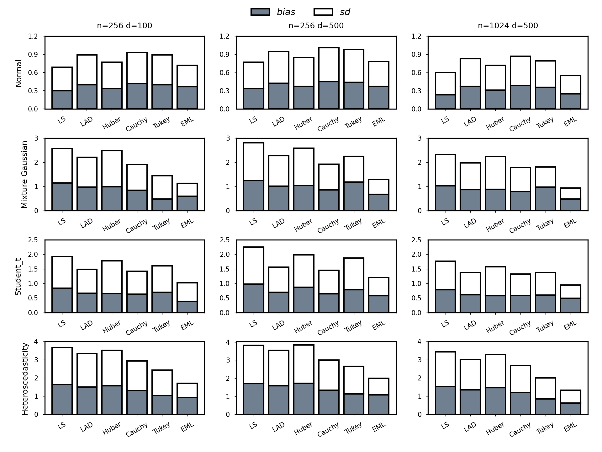
Figure 1: The bar chart of the bias and standard deviation of $g_{5}$ using six methods for four error distributions with sample sizes $n=256,1024$ and input dimensions $d=100,500$, respectively.

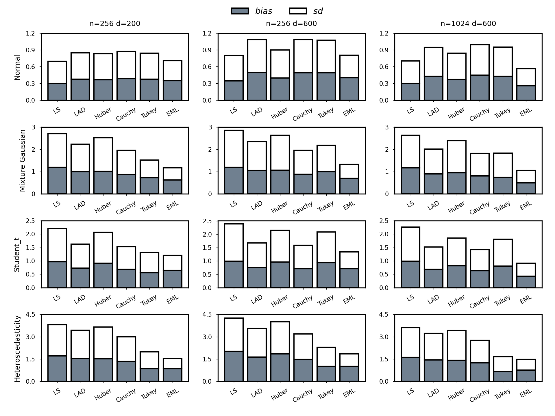
Figure 2: The bar chart of the bias and standard deviation of $g_{10}$ using six methods for four error distributions with sample sizes $n=256,1024$ and input dimensions $d=200,600$, respectively.

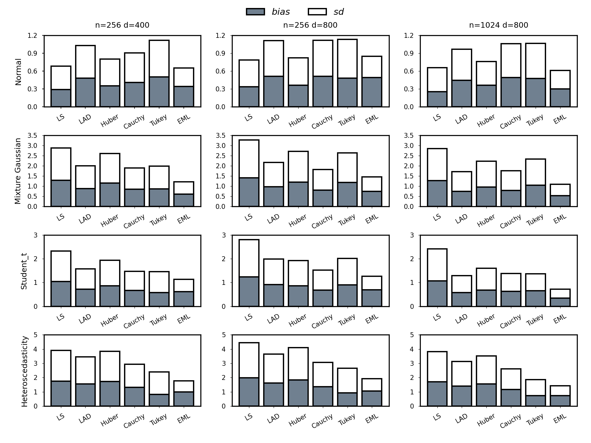
Figure 3: The bar chart of the bias and standard deviation of $g_{20}$ using six methods for four error distributions with sample sizes $n=256,1024$ and input dimensions $d=400,800$, respectively.

4.3 Effect of the bandwidth

Now, we examine the effect of bandwidth on the proposed method. In Figures 4 and 5, we present the bias, SD, and prediction error (PE) of the EML-FNN estimator when the bandwidths vary from 0.2 to 0.8 for $g_{5}$ under four error distributions given $(n,d)=(1024,500)$. PE is defined as $PE=\frac{1}{t}\sum_{i=1}^{t}\left\|g(X_{i}^{test})-Y_{i}^{test}\right\|^{2}$, where $\left\{(X_{i}^{test},Y_{i}^{test}\right\}_{i=1}^{t}$ represents the test data, which shares the same distribution as the training data. From Figures 4 and 5, we can see that a smaller bandwidth provides a better estimator in terms of bias, SD, and PE, and the proposed EML estimator is robust to variations in bandwidth within a certain range that approaches zero. These findings are consistent with the theoretical result presented in Theorem 2, which indicates that a small bandwidth is favored, and the extra risk is independent of the bandwidth if the bandwidth is appropriately small. Additionally, the comparison of Figures 4 and 5 reveals that the PE is more stable than bias and SD as the bandwidth changes.

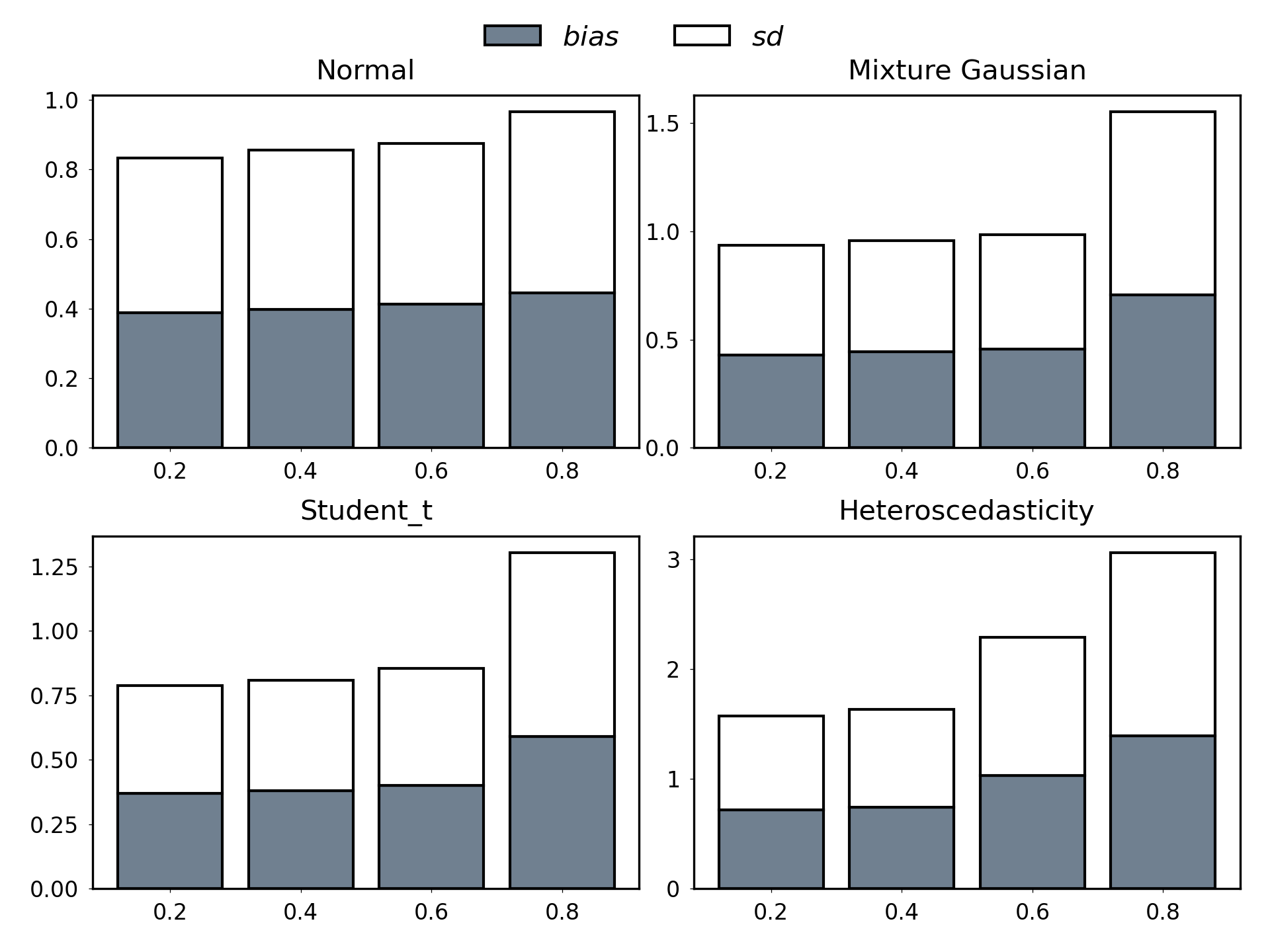
Figure 4: The bar chart of the bias and standard deviation of the proposed EML-FNN for $g_{5}$ under four error distributions with $(n,d)=(1024,500)$, as the bandwidths vary from 0.2 to 0.8.

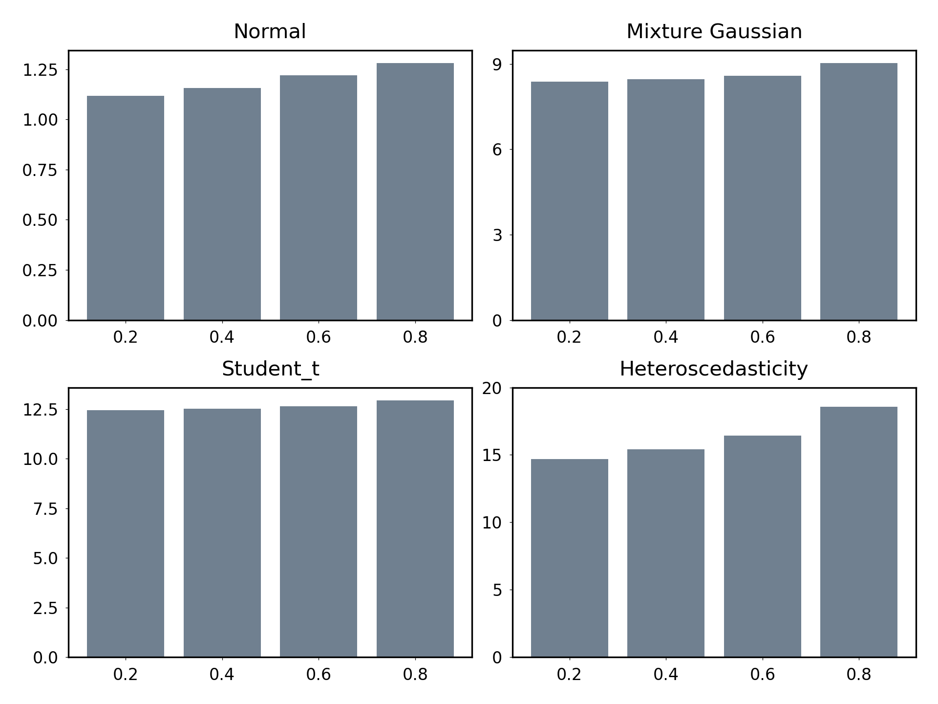
Figure 5: The bar chart of the mean prediction error (PE) of the proposed EML-FNN for $g_{5}$ under four error distributions with $(n,d)=(1024,500)$, as the bandwidths vary from 0.2 to 0.8.

5 Real data example

We applied our proposed EML-FNN and other competing methods to analyze four real datasets based on the model (1) using the observations $(\bm{X}_{i},Y_{i})_{i=1}^{n}$.

• Boston House Price Dataset. It is available in the scikit-learn library (Pedregosa et al., 2011) and encompasses a total of $n=506$ observations. The purpose of the analysis is predicting the house price based on the 13 input variables $\bm{X}_{i}$, such as urban crime rates, nitric oxide levels, average number of rooms in a dwelling, weighted distance to central areas, and average owner-occupied house prices, among others. Following Kong and Xia, (2012) and Zhou et al., (2019), we employ the logarithm of the median price of owner-occupied residences in units of $1,000 as our response $Y_{i}$.

• QSAR aquatic toxicity Dataset. The dataset was provided by Cassotti et al., (2014) and was used to develop quantitative regression QSAR models for predicting acute aquatic toxicity towards Daphnia Magna. It consists of a total of $n=546$ observations, each has 8 molecular descriptors serving as covariates $\bm{X}_{i}$, including PSA(Tot) (Molecular properties), SAacc (Molecular properties), H-050 (Atom-centred fragments), MLOGP (Molecular properties), RDCHI (Connectivity indices), GATS1p (2D autocorrelations), nN (Constitutional indices), C-040 (Atom-centred fragments). The response variable $Y_{i}$ is the acute aquatic toxicity, specifically the LC50, which is defined as the concentration causing death in 50% of the test D. magna over a test duration of 48 hours.

• QSAR fish toxicity Dataset. Another version of the dataset for quantitative regression QSAR models was provided by Cassotti et al., (2015). This dataset includes 908 observations, each observation has 6 input variables ($\bm{X}_{i}$) including molecular descriptors: MLOGP (molecular properties), CIC0 (information indices), GATS1i (2D autocorrelations), NdssC (atom-type counts), NdsCH ((atom-type counts), SM1_Dz(Z) (2D matrix-based descriptors). The response variable $Y_{i}$ is the LC50 which is the concentration that causes death in 50% of test fish over a test duration of 96 hours.

• Temperature forecast Dataset. The dataset was provided by Cho et al., (2020) and aims to correcting bias of next-day maximum and minimum air temperatures forecast from the LDAPS model operated by the Korea Meteorological Administration over Seoul, South Korea. The data consists of summer data spanning from 2013 to 2017. The input data $\bm{X}_{i}$ is largely composed of predictions from the LDAPS model for the subsequent day, in-situ records of present-day maximum and minimum temperatures, and five geographic auxiliary variables. In this dataset, two outputs ($Y_{i}$) are featured: next-day maximum and minimum air temperatures.

Table 1: Mean prediction error for four real datasets.

	Boston	Aquatic Toxicity	Fish Toxicity
	(Pedregosa et al., 2011)	(Cassotti et al., 2014)	(Cassotti et al., 2015)
LS	0.1045	1.2812	2.0153
LAD	0.1054	1.2184	2.142
Huber	0.1155	1.2003	2.1403
Cauchy	0.1192	1.2697	2.1179
Tukey’s biweight	0.1153	1.3148	2.1436
EML	0.0833	1.1497	1.8918
	Temperature Forecast
	(Cho et al., 2020)
LS	10.9303	5.5969
LAD	10.6615	5.71
Huber	10.6054	5.3211
Cauchy	11.4592	6.0396
Tukey’s biweight	11.2879	5.2332
EML	4.4085	2.2196

We preprocessed all the datasets by applying Z-score normalization to each predictor variable. Inspired from transfer learning, we employed the widely-used fine-tuning technique to simplify the computation. We initiated the process by training a single network model based on, for example, the Cauchy loss function by employing the methodology outlined in Section 4. Subsequently, we leveraged this trained model as a foundation to train all other models with a learning rate of $0.00003$. All four datasets were randomly split into training and test sets with a ratio of 4:1 to calculate PE. The entire procedure was repeated 50 times, and the average PE were calculated and presented in Table 1. The results in Table 1 clearly demonstrate the significant superiority of our approach over other competing methods in terms of a remarkable improvement in prediction accuracy across all four datasets. Particularly noteworthy is the outstanding performance achieved when applying our proposed EML technique to the Temperature Forecast dataset, where the improvement of the prediction accuracy achieves up to $50\%$. To understand the underlying reasons behind this improvement, we proceeded to plot the Q-Q plot in Figure 6 on the estimated error distribution for each of four real datasets. From the Q-Q plot in Figure 6, we can see the distribution of Boston house prices quite close to normal distribution. Following this, the toxicity data exhibits relatively closer resemblance to normality, characterized by a limited number of outliers. In contrast, the temperature data diverges substantially from the normal distribution, with a notable prevalence of extreme values. Based on these findings, we can draw the conclusion that the prediction performances, as illustrated in Table 1, are linked to the degree to which the respective distributions adhere to normality. Furthermore, from Tables 1 and Figure 6, we also can see that all the methods exhibit enhanced predictive accuracy when handling datasets that are more similar to a normal distribution. This observation further highlights the influence of distribution characteristics on the resulting estimator and emphasizes the importance of incorporating distribution information into the analysis.

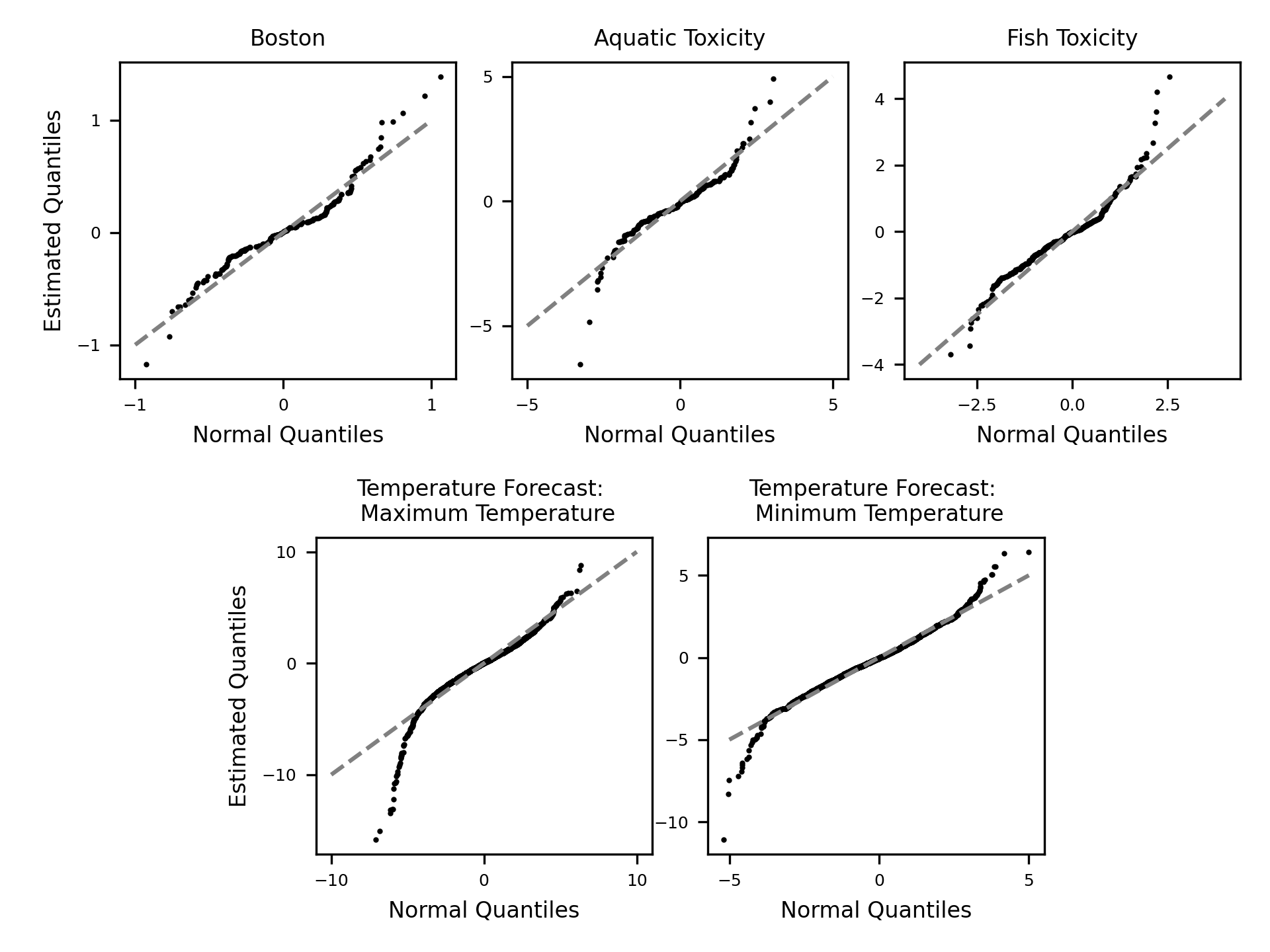
Figure 6: The Q-Q plot of the estimated density function for four real datasets.

6 Concluding Remarks

The paper presents an innovative approach to nonparametric regression using FNN. This approach is characterized by its efficiency in both estimation and computation, its adaptability to diverse data distributions, and its robustness in the presence of noise and uncertainty. The key contributions are as follows: (1) Estimation efficiency: The method introduces a novel loss function that incorporates not only observed data but also potentially implicit information about the data structure. By integrating this hidden information, the loss function transforms into an estimated maximum likelihood function, resulting in desirable properties such as efficiency. (2) Distribution-free: The method is independent of data distribution assumptions. Consequently, the approach adeptly handles data with varying distributional characteristics, such as heavy tails, multimodal distributions, and heterogeneity. (3) Probabilistic Robustness: The loss function is formulated through a probabilistic framework. This probabilistic approach effectively reduce the impact of substantial noise and outliers within the data, thereby enhancing its robustness. (4) Kernel-Based Smoothness: The method leverages the inherent smoothness of kernel functions. This enables the calculation of gradients and addresses challenges related to non-differentiability, when dealing with densities such as uniform distributions, mixture distributions, and cases of heteroscedasticity. (5) Computational efficiency: The proposed loss function exclusively involves the regression function $g$. This design facilitates the straightforward utilization of existing software packages, simplifying the computational and programming. In summary, the method’s capacity to accommodate various data distributions without the need for distributional assumptions renders it versatile and applicable to a wide range of real-world scenarios.

By utilizing a reasonably small bandwidth, the proposed estimator is proved to be equivalent to the maximum likelihood estimator (MLE) where the density function is known. Furthermore, it nearly attains the minimax optimal rate, with only an additional logarithmic factor. Its exceptional performance is further exemplified through comprehensive simulation studies and its successful application to four distinct real-world datasets.

There are several directions for future research. First, it might be possible to extend our method to a more complicated model, such as the generalized regression model for a discrete response. Secondly, practical scenarios often involve multiple responses that exhibit correlations, as seen in the Temperature Forecast Dataset’s maximum and minimum air temperatures. By further modeling inter-response correlations, predictive capabilities could be enhanced. Lastly, it remains our responsibility to consistently enhance the associated software packages, ensuring seamless application. Despite having introduced an efficient and user-friendly package named EML-FNN, continued optimization and refinement are necessary.

References

- Bartlett et al., (2019) Bartlett, P. L., Harvey, N., Liaw, C., and Mehrabian, A. (2019). Nearly-tight vc-dimension and pseudodimension bounds for piecewise linear neural networks. The Journal of Machine Learning Research, 20(1):2285–2301.
- Bassett Jr and Koenker, (1978) Bassett Jr, G. and Koenker, R. (1978). Asymptotic theory of least absolute error regression. Journal of the American Statistical Association, 73(363):618–622.
- Bauer and Kohler, (2019) Bauer, B. and Kohler, M. (2019). On deep learning as a remedy for the curse of dimensionality in nonparametric regression. The Annals of Statistics, 47(4):2261–2285.
- Beaton and Tukey, (1974) Beaton, A. E. and Tukey, J. W. (1974). The fitting of power series, meaning polynomials, illustrated on band-spectroscopic data. Technometrics, 16(2):147–185.
- Berlinet and Thomas-Agnan, (2011) Berlinet, A. and Thomas-Agnan, C. (2011). Reproducing kernel Hilbert spaces in probability and statistics. Springer Science & Business Media.
- Bhattacharya et al., (2023) Bhattacharya, S., Fan, J., and Mukherjee, D. (2023). Deep neural networks for nonparametric interaction models with diverging dimension. arXiv preprint arXiv:2302.05851.
- Breiman, (2001) Breiman, L. (2001). Random forests. Machine learning, 45:5–32.
- Breiman, (2017) Breiman, L. (2017). Classification and regression trees. Routledge.
- Cassotti et al., (2014) Cassotti, M., Ballabio, D., Consonni, V., Mauri, A., Tetko, I. V., and Todeschini, R. (2014). Prediction of acute aquatic toxicity toward daphnia magna by using the ga-k nn method. Alternatives to Laboratory Animals, 42(1):31–41.
- Cassotti et al., (2015) Cassotti, M., Ballabio, D., Todeschini, R., and Consonni, V. (2015). A similarity-based qsar model for predicting acute toxicity towards the fathead minnow (pimephales promelas). SAR and QSAR in Environmental Research, 26(3):217–243.
- Chen et al., (2019) Chen, M., Jiang, H., Liao, W., and Zhao, T. (2019). Nonparametric regression on low-dimensional manifolds using deep relu networks: Function approximation and statistical recovery. arXiv preprint arXiv:1908.01842.
- Cheng, (1984) Cheng, P. E. (1984). Strong consistency of nearest neighbor regression function estimators. Journal of Multivariate Analysis, 15(1):63–72.
- Cho et al., (2020) Cho, D., Yoo, C., Im, J., and Cha, D.-H. (2020). Comparative assessment of various machine learning-based bias correction methods for numerical weather prediction model forecasts of extreme air temperatures in urban areas. Earth and Space Science, 7(4):e2019EA000740.
- Cleveland, (1979) Cleveland, W. S. (1979). Robust locally weighted regression and smoothing scatterplots. Journal of the American statistical association, 74(368):829–836.
- Devroye et al., (1994) Devroye, L., Gyorfi, L., Krzyzak, A., and Lugosi, G. (1994). On the strong universal consistency of nearest neighbor regression function estimates. The Annals of Statistics, 22(3):1371–1385.
- Donoho et al., (1995) Donoho, D. L., Johnstone, I. M., Kerkyacharian, G., and Picard, D. (1995). Wavelet shrinkage: asymptopia? Journal of the Royal Statistical Society: Series B (Methodological), 57(2):301–337.
- Fan and Gijbels, (2018) Fan, J. and Gijbels, I. (2018). Local polynomial modelling and its applications. Routledge.
- Fan and Gu, (2022) Fan, J. and Gu, Y. (2022). Factor augmented sparse throughput deep relu neural networks for high dimensional regression. arXiv preprint arXiv:2210.02002.
- Fan et al., (2022) Fan, J., Gu, Y., and Zhou, W.-X. (2022). How do noise tails impact on deep relu networks? arXiv preprint arXiv:2203.10418.
- Farrell et al., (2021) Farrell, M. H., Liang, T., and Misra, S. (2021). Deep neural networks for estimation and inference. Econometrica, 89(1):181–213.
- Györfi et al., (2002) Györfi, L., Kohler, M., Krzyzak, A., Walk, H., et al. (2002). A distribution-free theory of nonparametric regression, volume 1. Springer.
- Hall and Huang, (2001) Hall, P. and Huang, L.-S. (2001). Nonparametric kernel regression subject to monotonicity constraints. The Annals of Statistics, 29(3):624–647.
- Härdle, (1989) Härdle, W. (1989). Asymptotic maximal deviation of m-smoothers. Journal of Multivariate Analysis, 29(2):163–179.
- He et al., (2015) He, K., Zhang, X., Ren, S., and Sun, J. (2015). Delving deep into rectifiers: Surpassing human-level performance on imagenet classification. In 2015 IEEE International Conference on Computer Vision (ICCV), pages 1026–1034.
- He et al., (2013) He, X., Wang, L., and Hong, H. G. (2013). Quantile-adaptive model-free variable screening for high-dimensional heterogeneous data. The Annals of Statistics, 41(1):342–369.
- Huber, (1973) Huber, P. J. (1973). Robust Regression: Asymptotics, Conjectures and Monte Carlo. The Annals of Statistics, 1(5):799 – 821.
- Jiao et al., (2021) Jiao, Y., Shen, G., Lin, Y., and Huang, J. (2021). Deep nonparametric regression on approximately low-dimensional manifolds. arXiv preprint arXiv:2104.06708.
- Kingma and Ba, (2014) Kingma, D. P. and Ba, J. (2014). Adam: A method for stochastic optimization. arXiv preprint arXiv:1412.6980.
- Koenker and Bassett Jr, (1978) Koenker, R. and Bassett Jr, G. (1978). Regression quantiles. Econometrica, 46(1):33–50.
- Kohler et al., (2022) Kohler, M., Krzyzak, A., and Langer, S. (2022). Estimation of a function of low local dimensionality by deep neural networks. IEEE transactions on information theory, 68(6):4032–4042.
- Kohler and Langer, (2021) Kohler, M. and Langer, S. (2021). On the rate of convergence of fully connected deep neural network regression estimates. The Annals of Statistics, 49(4):2231–2249.
- Kong and Xia, (2012) Kong, E. and Xia, Y. (2012). A single-index quantile regression model and its estimation. Econometric Theory, 28(4):730–768.
- Lederer, (2020) Lederer, J. (2020). Risk bounds for robust deep learning. arXiv preprint arXiv:2009.06202.
- Liu et al., (2022) Liu, R., Boukai, B., and Shang, Z. (2022). Optimal nonparametric inference via deep neural network. Journal of Mathematical Analysis and Applications, 505(2):125561.
- Loftsgaarden and Quesenberry, (1965) Loftsgaarden, D. O. and Quesenberry, C. P. (1965). A nonparametric estimate of a multivariate density function. The Annals of Mathematical Statistics, 36(3):1049–1051.
- Lu et al., (2021) Lu, J., Shen, Z., Yang, H., and Zhang, S. (2021). Deep network approximation for smooth functions. SIAM Journal on Mathematical Analysis, 53(5):5465–5506.
- Lv et al., (2018) Lv, S., Lin, H., Lian, H., and Huang, J. (2018). Oracle inequalities for sparse additive quantile regression in reproducing kernel hilbert space. The Annals of Statistics, 46(2):781–813.
- Nadaraya, (1964) Nadaraya, E. A. (1964). On estimating regression. Theory of Probability & Its Applications, 9(1):141–142.
- Nakada and Imaizumi, (2019) Nakada, R. and Imaizumi, M. (2019). Adaptive approximation and estimation of deep neural network to intrinsic dimensionality. arXiv preprint arXiv:1907.02177, 6.
- Onzon, (2011) Onzon, E. (2011). Multivariate cramér–rao inequality for prediction and efficient predictors. Statistics & probability letters, 81(3):429–437.
- Padilla et al., (2020) Padilla, O. H. M., Tansey, W., and Chen, Y. (2020). Quantile regression with deep relu networks: Estimators and minimax rates. arXiv preprint arXiv:2010.08236.
- Paszke et al., (2019) Paszke, A., Gross, S., Massa, F., Lerer, A., Bradbury, J., Chanan, G., Killeen, T., Lin, Z., Gimelshein, N., Antiga, L., et al. (2019). Pytorch: An imperative style, high-performance deep learning library. Advances in neural information processing systems, 32.
- Pedregosa et al., (2011) Pedregosa, F., Varoquaux, G., Gramfort, A., Michel, V., Thirion, B., Grisel, O., Blondel, M., Prettenhofer, P., Weiss, R., Dubourg, V., Vanderplas, J., Passos, A., Cournapeau, D., Brucher, M., Perrot, M., and Duchesnay, E. (2011). Scikit-learn: Machine learning in Python. Journal of Machine Learning Research, 12:2825–2830.
- Schmidt-Hieber, (2019) Schmidt-Hieber, J. (2019). Deep relu network approximation of functions on a manifold. arXiv preprint arXiv:1908.00695.
- Schmidt-Hieber, (2020) Schmidt-Hieber, J. (2020). Nonparametric regression using deep neural networks with relu activation function. The Annals of Statistics, 48(4):1875–1897.
- Schumaker, (2007) Schumaker, L. (2007). Spline functions: basic theory. Cambridge university press.
- (47) Shen, G., Jiao, Y., Lin, Y., Horowitz, J. L., and Huang, J. (2021a). Deep quantile regression: Mitigating the curse of dimensionality through composition. arXiv preprint arXiv:2107.04907.
- (48) Shen, G., Jiao, Y., Lin, Y., and Huang, J. (2021b). Robust nonparametric regression with deep neural networks. arXiv preprint arXiv:2107.10343.
- Shen et al., (2019) Shen, Z., Yang, H., and Zhang, S. (2019). Deep network approximation characterized by number of neurons. arXiv preprint arXiv:1906.05497.
- Stone, (1977) Stone, C. J. (1977). Consistent nonparametric regression1. The Annals of Statistics, 5(4):595–620.
- Stone, (1982) Stone, C. J. (1982). Optimal global rates of convergence for nonparametric regression. Ann. Statist., 10(1):1040–1053.
- Tukey et al., (1977) Tukey, J. W. et al. (1977). Exploratory data analysis, volume 2. Reading, MA.
- Wang and Scott, (1994) Wang, F. T. and Scott, D. W. (1994). The l 1 method for robust nonparametric regression. Journal of the American Statistical Association, 89(425):65–76.
- Watson, (1964) Watson, G. S. (1964). Smooth regression analysis. Sankya, Series A, 26:359–372.
- Yan and Yao, (2023) Yan, S. and Yao, F. (2023). Nonparametric regression for repeated measurements with deep neural networks. arXiv preprint arXiv:2302.13908.
- Yarotsky, (2017) Yarotsky, D. (2017). Error bounds for approximations with deep relu networks. Neural Networks, 94:103–114.
- Zhou et al., (2019) Zhou, L., Lin, H., Chen, K., and Liang, H. (2019). Efficient estimation and computation of parameters and nonparametric functions in generalized semi/non-parametric regression models. Journal of Econometrics, 213(2):593–607.
- Zhou et al., (2018) Zhou, L., Lin, H., and Liang, H. (2018). Efficient estimation of the nonparametric mean and covariance functions for longitudinal and sparse functional data. Journal of the American Statistical Association, 113(524):1550–1564.