Penalty Ensembles for Navier-Stokes with Random Initial Conditions & Forcing

Abstract

Inspired by the novel ensemble method for the Navier-Stokes equations (NSE) in 2014 Nan-Layton-ensemble , and the work of YanLuo-ZhuWang-ensemble , this report develops an ensemble penalty method for the NSE. In addition, the method is extended to the Monte Carlo random sampling. The combination allows greater ensemble sizes with reduced complexity and thus gives a longer predictability horizon.

1 Introduction

In many applications uncertainty in problem data occurs. Then one is interested in simulations with different initial conditions and boundary conditions, body forces and other data Kalnay . This leads to a number of simulations and that are computationally expensive. Also with different initial conditions trajectories spread. When they are $\mathbf{O}(1)$ apart, the prediction will not be useful Lorenz . To extend their prediction ability, we compute ensembles, $u_{j},p_{j}$ of solutions of the NSE:

$$\begin{split}&u_{j,t}+u_{j}\cdot\nabla u_{j}-\nu\Delta u_{j}+\nabla p_{j}=f_{j}(x,t),\quad\text{ in }\Omega,j=1\cdots J,\\ &\nabla\cdot u_{j}=0,\text{ and }u_{j}(x,0)=u^{0}_{j}(x)\in\Omega,\text{ on }u_{j}=0\text{ on }\partial\Omega.\end{split}$$ (1)

The best prediction is the ensemble average and the predictability horizon is proportional to the ensemble spread. The velocity $u_{j}$ and pressure $p_{j}$ in the above equations are coupled together by the incompressible constraint. Penalty method replace

$$\nabla\cdot u_{j}=0\text{ with }\nabla\cdot u^{\epsilon}_{j}+\epsilon p_{j}^{\epsilon}=0,\text{ for }\epsilon<<1$$

to relax incompressibility. The result is the following: let $(x,t)\in\Omega\times[0,T]$,

$$\begin{split}&u^{\epsilon}_{j,t}+B(u_{j}^{\epsilon},u_{j}^{\epsilon})-\nu\Delta u^{\epsilon}_{j}+\nabla p^{\epsilon}_{j}=f_{j}(x,t),\quad\nabla\cdot u^{\epsilon}_{j}+\epsilon p^{\epsilon}_{j}=0,\end{split}$$ (2)

where

$$B(u,v)=(u\cdot\nabla)v+\frac{1}{2}(\nabla\cdot u)v,$$

and

$$\begin{split}u^{\epsilon}_{j}=0,\quad(x,t)\in\partial\Omega\times(0,T],\text{ and }u^{\epsilon}_{j}(x,0)=u^{0}_{j}(x),\quad x\in\Omega.\end{split}$$ (3)

The $B(u,v)$ term was introduced by Temam Temam-energey-dissipation . He proved in Temam-energey-dissipation that

$$\lim_{\epsilon\to 0}(u_{j},p_{j})=(u^{\epsilon}_{j},p^{\epsilon}_{j}).$$

Execution needs to assemble and solve $J$ linear systems at each timestep. To increase efficiency, we adapt ensemble methods to the penalty NSE from Nan-Layton-ensemble .

Denote the ensemble mean and fluctuation by

$$\begin{split}&<u^{\epsilon}>^{n}:=\frac{1}{J}\sum_{j=1}^{J}u^{\epsilon,n}_{j},\text{ and }U^{\epsilon,n}_{j}:=u^{\epsilon,n}_{j}-<u^{\epsilon}>^{n},\end{split}$$

and the usual explicitly skew symmetric trilinear form by

$$b^{*}(u,v,w):=\frac{1}{2}(u\cdot\nabla v,w)-\frac{1}{2}(u\cdot\nabla w,v).$$

To present the idea, suppress the spatial discretization. Using an implicit-explicit time discretization and keeping the resulting coefficient matrix independent of the ensemble member, leads to the method: for $(x,t)\in\Omega\times[0,T]$:

$$\begin{split}\frac{u^{\epsilon,n+1}_{j}-u^{\epsilon,n}_{j}}{\Delta t}+B(<u^{\epsilon}>^{n},u_{j}^{\epsilon,n+1})+&B(U^{\epsilon,n}_{j},u^{\epsilon,n}_{j})-\nu\Delta u_{j}^{\epsilon,n+1}+\nabla p^{\epsilon,n+1}_{j}=f_{j}^{n+1},\\ \nabla\cdot u_{j}^{\epsilon,n+1}+&\epsilon p_{j}^{\epsilon,n+1}=0.\end{split}$$ (4)

Here $\epsilon$ must be the same across all ensemble members to reduce memory required by eliminating the pressure and sharing the coefficient matrix among realizations.

2 Algorithms

Let $\Omega$ be an open regular domain in $\mathbb{R}^{d}$ ($d=2$ or 3). Let $X^{h}$ and $Q^{h}$ be the conforming finite element space of the velocity and the pressure respectively:

$$X^{h}\subset X:=(H^{1}_{0}(\Omega))^{d},\quad Q^{h}\subset Q:=L^{2}_{0}(\Omega)).$$

We assume that $X^{h}$ and $Q^{h}$ satisfy the usual inf-sup condition. Let $T$ be the final time, and $\Delta t_{n}$ denote the timestep at the $n_{th}$ step. The final step $N=T/\Delta t$. The fully discrete approximation of the method is given $(u^{\epsilon,n}_{j,h},p^{\epsilon,n}_{j,h})\in(X^{h},Q^{h})$, find $(u^{\epsilon,n+1}_{j,h},p^{\epsilon,n+1}_{j,h})\in(X^{h},Q^{h})$ satisfying:

$$\begin{split}\frac{1}{\Delta t_{n}}(u^{\epsilon,n+1}_{j,h}-u^{\epsilon,n}_{j,h},v_{h})+b^{*}(<u^{\epsilon}_{h}>^{n},u^{\epsilon,n+1}_{j,h},v_{h})+b^{*}(u^{\epsilon,n}_{j,h}-<u^{\epsilon}_{h}>^{n},u^{\epsilon,n}_{j,h},v_{h})\\ +\nu(\nabla u^{\epsilon,n+1}_{j,h},\nabla v_{h})-(p^{\epsilon,n+1}_{j,h},\nabla\cdot v^{h})+(q^{h},\nabla\cdot u^{\epsilon,n+1}_{j,h})+\epsilon(p^{\epsilon,n+1}_{j,h},q^{h})=(f_{j}^{n+1},v_{h}),\end{split}$$ (5)

for all $(v^{h},q^{h})\in(X^{h},Q^{h})$.

By solving the ensemble members with a shared coefficient matrix and different right-hand side vectors, we can reduce computation time greatly. Due to the explicit discretization of the stretching term $b^{*}(u^{\epsilon,n}_{j,h}-<u^{\epsilon}_{h}>^{n},u^{\epsilon,n}_{j,h},v_{h})$, the CFL timestep restriction is necessary:

$$C\frac{\Delta t}{\nu h}\|\nabla(u_{j}-<u>)\|^{2}\leq 1.$$

Algorithm 1

$\Delta t$, $\epsilon$, $u^{n}$, and $u^{n}_{j},j=1,\cdots,J$ at time $t$.

while $t<T$ do:

     Compute the average $<u>^{n}=\frac{1}{J}\sum_{j=1}^{J}u^{n}_{j}$.

     Solve the next step velocity $u^{n+1}_{j}$ by the method in (5).

     Update the average $<u>^{n+1}=\frac{1}{J}\sum_{j=1}^{J}u^{n+1}_{j}$.

     Calculate $\max_{j}\|\nabla(u^{n+1}_{j}-<u>^{n+1})\|$ and verify the CFL condition.

     if the CFL condition is satisfied then

         update time by $t=t+\Delta t$. $\triangleright$ Succeed, and go to next timestep

     else

         $\Delta t=\frac{1}{2}\Delta t$.

     end if

end while

3 Error Analysis

In this section, we summarize stability and convergence theorems from our analysis. We assume:

$$\begin{split}\inf_{v\in X^{h}}\|u-v\|\leq Ch^{m+1}|u|_{m+1},\quad u\in H^{m+1}(\Omega)^{d},\\ \inf_{v\in X^{h}}\|\nabla(u-v)\|\leq Ch^{m}|u|_{m+1},\quad u\in H^{m+1}(\Omega)^{d},\\ \inf_{q\in Q^{h}}\|p-q\|\leq Ch^{m}|p|_{m},\quad p\in H^{m}(\Omega).\end{split}$$ (6)

Theorem 3.1

(Stability) Under the CFL condition, for any $N>1$:

$$\frac{1}{2}\|u^{\epsilon,N}_{j,h}\|^{2}+\frac{1}{4}\sum_{n=0}^{N-1}\|u^{\epsilon,n+1}_{j,h}-u^{\epsilon,n}_{j,h}\|^{2}+\frac{\nu\Delta t}{4}\|\nabla u^{\epsilon,N}_{j,h}\|^{2}$$

$$+\frac{\nu\Delta t}{4}\sum_{n=0}^{N-1}\|\nabla u^{\epsilon,n+1}_{j,h}\|^{2}+\frac{\Delta t}{\epsilon}\sum_{n=0}^{N-1}\|P_{Q^{h}}(\nabla\cdot u^{\epsilon,n+1}_{j,h})\|^{2}$$

$$\leq\frac{\Delta t}{2\nu}\sum_{n=0}^{N-1}\|f^{n+1}_{j}\|^{2}_{-1}+\frac{1}{2}\|u^{0}_{j,h}\|^{2}+\frac{\nu\Delta t}{4}|\|\nabla u^{0}_{j,h}\|^{2},$$

where $P_{Q^{h}}$ is the L2-orthogonal projection.

Theorem 3.2

(Convergence) Under the CFL condition for regular solutions, we have the following optimal estimates:

$$\sup_{1\leq n\leq N}\tau(t_{n})\|\nabla u_{j}(t_{n})-\nabla u^{\epsilon,n}_{j,h}\|\leq C(\epsilon+\Delta t+h^{m}),\text{where }\tau(t)=\min\{t,1\}.$$

4 Numerical Experiments

We present numerical experiments of the algorithm with simply $J=2$ ensemble members. In the first test, we applied perturbations on the initial conditions of the Green-Taylor vortex. We verified the accuracy of the algorithm and confirmed the predicted convergence rates. In the second test, we studied a rotating flow on offset cylinders. Adapting the timestep, kinetic energy, angular momentum, and enstrophy indicated that stability was preserved.

4.1 Convergence Experiment

The Green-Taylor vortex problem is commonly used for convergence rates, since the analytical solution is known Volker . In $\Omega=(0,1)^{2}$, the exact solution of the Green-Taylor vortex is

$$\begin{split}u(x,y,t)&=-cos(x)sin(y)sin(t)\\ v(x,y,t)&=sin(x)cos(y)sin(t)\\ p(x,y,t)&=\frac{1}{4}\left(cos(2x)+cos(2y)\right)sin^{2}(t)\end{split}$$

We take the exact initial solutions, with perturbed initial conditions

$$\begin{split}u^{0}_{1}=(1+\epsilon_{1})u^{0},\ u^{0}_{2}=(1+\epsilon_{2})u^{0},\text{ where }\delta_{1}=10^{-3},\delta_{2}=-10^{-3}.\end{split}$$

We take $\nu=1,\mathcal{R}e=1/\nu,h=1/m$, and $\Delta t=1/10h$, penalty parameter $\epsilon=\Delta t$. Denote error $e(h)=Ch^{\beta}$, solve $\beta$ via

$$\beta=\frac{ln(e(h1)/e(h2))}{ln(h_{1}/h_{2})}$$

at two successive values of $h$. Set inhomogeneous Dirichlet boundary condition $u_{h}=u_{true}\text{ on }\partial\Omega.$

Table 1: Errors and convergence rates for $u_{1}$.

m	$\max_{t_{n}}\|u_{1}-u_{1,h}\|_{2,0}$	rate	$\int_{0}^{T}\|\nabla u_{1}-\nabla u_{1,h}\|_{2,0}$	rate
$(\frac{3}{2})^{0}\cdot 27$	$1.38318\cdot 10^{-4}$	–	$3.61255\cdot 10^{-4}$	–
$(\frac{3}{2})^{1}\cdot 27$	$9.37671\cdot 10^{-5}$	0.98906199	$2.38614\cdot 10^{-4}$	1.05519213
$(\frac{3}{2})^{2}\cdot 27$	$6.26996\cdot 10^{-5}$	0.99258689	$1.57337\cdot 10^{-4}$	1.02711214
$(\frac{3}{2})^{3}\cdot 27$	$4.14256\cdot 10^{-5}$	0.99505826	$1.03233\cdot 10^{-4}$	1.01173507
$(\frac{3}{2})^{4}\cdot 27$	$2.77552\cdot 10^{-5}$	0.99671009	$6.89522\cdot 10^{-5}$	1.00442624

Table 2: Errors and convergence rates for $u_{2}$.

m	$\max_{t_{n}}\|u_{2}-u_{2,h}\|_{2,0}$	rate	$\int_{0}^{T}\|\nabla u_{2}-\nabla u_{2,h}\|_{2,0}$	rate
$(\frac{3}{2})^{0}\cdot 27$	$1.37767\cdot 10^{-4}$	–	$3.59895\cdot 10^{-4}$	–
$(\frac{3}{2})^{1}\cdot 27$	$9.33934\cdot 10^{-5}$	0.98906665	$2.37692\cdot 10^{-4}$	1.05544879
$(\frac{3}{2})^{2}\cdot 27$	$6.24496\cdot 10^{-5}$	0.99258983	$1.56720\cdot 10^{-4}$	1.0272543
$(\frac{3}{2})^{3}\cdot 27$	$4.12603\cdot 10^{-5}$	0.99506015	$1.02825\cdot 10^{-4}$	1.01180731
$(\frac{3}{2})^{4}\cdot 27$	$2.76446\cdot 10^{-5}$	0.99671132	$6.86788\cdot 10^{-5}$	1.00446153

Table 3: Errors and convergence rates for $u_{2}$.

We used the method (5) for the momentum equation and the P2 Lagrange element for the velocity. From Table 1 and Table 3, we can see that the convergence rates of $u_{1}$ and $u_{2}$ are first order as predicted.

4.2 Stability Verification

We test the timestep condition for stability on a flow between offset cylinders. We used the method (5) and the P2 Lagrange element for velocity. The domain is a disk with a smaller off-center obstacle inside. Let outer circle radius $r_{1}=1$ and inner circle radius $r_{2}=0.5$, $c=(c_{1},c_{2})=(\frac{1}{2},0)$. The domain is described as

$$\Omega=\{(x,y):x^{2}+y^{2}\text{ and }(x-c_{1})^{2}+(y-c_{2})^{2}\geq r_{2}^{2}\}.$$

The flow is driven by a counterclockwise rotational force

$$f(x,y,t)=(-4y(1-x^{2}-y^{2}),4x(1-x^{2}-y^{2}))^{T}$$

with no-slip boundary conditions. Note that the outer circle is remained stationary. The unstructured mesh was generated with GMSH, with GMSH target mesh size parameter $lc=0.05$ (1). We chose the final time $T=100$, timestep $\Delta t=lc/10,\nu=1/150,\mathcal{R}e=150$ and penalty parameter $\epsilon=\Delta t$.

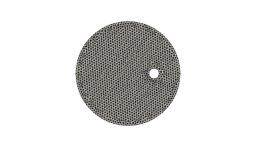
Figure 1: Mesh of the offset cylinder

Initial condition $u^{0}=0$, and $u=0$ on $\partial\Omega$. We perturbed initial condition with $\delta_{1}=0.1,\delta_{2}=-0.1$:

$$u^{0}_{j}:=\delta_{j}(1-x^{2}-y^{2})(0.5^{2}-(x-0.5)^{2}-y^{2}),$$

thus the no-slip boundary condition is preserved. We solve the NSE with the perturbed initial conditions which give us $u_{1}$ and $u_{2}$ respectively.

For the evaluation of flow statistics, we calculated the angular momentum, enstrophy, and kinetic energy:

$$|\text{angular momentum}| =|\int_{\Omega}\bar{x}\times\bar{u}\,d\bar{x}|,\text{enstrophy}=\frac{1}{2}\nu\|\nabla\times\bar{u}\|^{2},$$

$$\text{kinetic energy}=\frac{1}{2}\|\bar{u}\|^{2}$$

To ensure the algorithm is stable, we adapt $\Delta t$ to satisfy the CFL condition with $C=1200$ Nan-Layton-ensemble :

$$\frac{\Delta t}{h}\|\nabla(u_{j}-<u>)\|^{2}\leq\frac{1200}{\mathcal{R}e},\text{ where }j=1,2.$$

If the CFL condition (4.2) is violated, we cut $\Delta t$ by half, and repeat the process until (4.2) is satisfied.

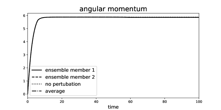
Figure 2: Stability: angular momentum, $\nu=1/150$.

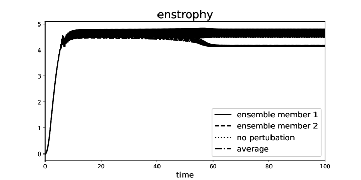
Figure 3: Stability: enstrophy, $\nu=1/150$.

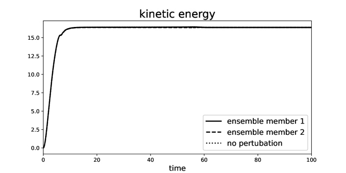
Figure 4: Stability: kinetic energy, $\nu=1/150$.

Figure 2 shows that the angular momentum aligns well for the ensemble members, and it is conserved, which indicates that the flow is stable. Enstrophy (Figure 3) is the integral of the vorticity square over the domain, and it measures the local rotation of a fluid. The enstrophy of the $u_{ave}$, the average of the ensemble members, is lower than the ensemble members and no perturbed one shows that the flow is smoothed out on average. In Figure 4, kinetic energy is very similar across all members and has reached a steady state.

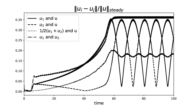
Figure 5: Spread with different initial conditions.

Figure 5 is the plot of the relative error, the ratio of the L2 norm of the difference and norm after the no perturbed flow reached a steady state.

When the $1^{st}$ significant digit is trustworthy, the difference of $u_{1}$ and $u_{2}$ indicates the predictability horizon of a single realization is about $T=30$, and the predictability horizon of the average, with two realizations is $T=50$. Our algorithm extends the predictability horizon.

5 Conclusions

In this report, we presented the stability and convergence of the ensemble penalty method (5) and verified the theorems are sharp with a suit of numerical tests. A larger ensemble size can give a more accurate and reliable simulation. We also extend the theorems to the Monte Carlo methods. Future work will extend this to a higher Reynolds number, and we are pursuing it now.

References

• (1) N. Jiang and W. Layton. ”An Algorithm for Fast Calculation of Flow Ensembles”, International Journal for Uncertainty Quantification, 4 (2014), 273-301.
• (2) Luo, Yan and Wang, Zhu. (2017). An Ensemble Algorithm for Numerical Solutions to Deterministic and Random Parabolic PDEs. SIAM Journal on Numerical Analysis. 56. 10.1137/17M1131489.
• (3) Kalnay, Eugenia. Atmospheric modeling, data assimilation and predictability. Cambridge university press, 2003.
• (4) Lorenz, E. N. ”The growth of errors in prediction.” Proceedings of the International School of Physics Enrico Fermi Course 88 on Turbulence and Predictability in Geophysical Fluid Dynamics and Climate Dynamics (1985).
• (5) Temam, R. Une mΓ©thode d’approximation de la solution des Γ©quations de Navier-Stokes. Bulletin de la SociΓ©tΓ© MathΓ©matique de France, Volume 96 (1968), pp. 115-152. doi : 10.24033/bsmf.1662. http://www.numdam.org/articles/10.24033/bsmf.1662/
• (6) John, Volker. Finite element methods for incompressible flow problems. Vol. 51. Cham: Springer International Publishing, 2016