Bridging Sensor Gaps via Single-Direction Tuning for Hyperspectral Image Classification

Abstract

Recently, vision transformer (ViT) models have excelled in diverse vision tasks, emerging as robust alternatives to convolutional neural networks. Inspired by this, some researchers have started exploring the use of ViTs in tackling HSI classification and achieved remarkable results. However, the training of ViT models requires a considerable number of training samples, while hyperspectral data, due to its high annotation costs, typically has a relatively small number of training samples. This contradiction has not been effectively addressed. In this paper, aiming to solve this problem, we propose the single-direction tuning (SDT) strategy, which serves as a bridge, allowing us to leverage existing labeled HSI datasets even RGB datasets to enhance the performance on new HSI datasets with limited samples. The proposed SDT inherits the idea of prompt tuning, aiming to reuse pre-trained models with minimal modifications for adaptation to new tasks. But unlike prompt tuning, SDT is custom-designed to accommodate the characteristics of HSIs. The proposed SDT utilizes a parallel architecture, an asynchronous cold-hot gradient update strategy, and unidirectional interaction. It aims to fully harness the potent representation learning capabilities derived from training on heterologous, even cross-modal datasets. In addition, we also introduce a novel Triplet-structured transformer (Tri-Former), where spectral attention and spatial attention modules are merged in parallel to construct the token mixing component for reducing computation cost and a 3D convolution-based channel mixer module is integrated to enhance stability and keep structure information. Comparison experiments conducted on three representative HSI datasets captured by different sensors demonstrate the proposed Tri-Former achieves better performance compared to several state-of-the-art methods. Homologous, heterologous and cross-modal tuning experiments verified the effectiveness of the proposed SDT. Code will be released at: https://github.com/Cecilia-xue/Tri-Former.

I Introduction

Hyperpectral image (HSI) classification aims to identify each pixel in an image and assign it to a specific land-cover category, which plays a crucial role in earth observation applications [1, 2]. Compared with traditional RGB images which only record three bands of colors, HSI images have much more rich spectral information. HSI sensors capture hundreds of spectral bands, each corresponding to a specific wavelength range. As a result, HSI images can provide more detailed and fine-grained information about the composition and properties of objects in the observed scene, which is very helpful in distinguishing ground-cover objects. Therefore, the HSI classification technology is widely applied in various scenes, e.g., mineral exploration [3], plant stress detection [4], and environmental science [5], etc. However, such high-dimensional features, on one hand, are beneficial for classifying ground objects. On the other hand, they also pose challenges in feature extraction due to their increased complexity. Hence, it is worthwile to explore efficient methods for feature extraction from raw HSIs.

Deep learning (DL) technique is famous for its superior ability to automatically extract deep features, which exactly meet the requirement of HSI classification. Over the past decade, DL based methods, especially convolutional neural network (ConvNet) based methods dominate the field of HSI classification. From 2013 to 2017, various DL based models have been proposed. For instance, in [6], Lin et al. utilized PCA to reduce the dimensionality of HSI from hundreds of spectral dimensions to dozens, then extract deep features from a neighborhood region via Stacked Autoencoder (SAE). Later, Chen et al. introduced another spectral channel to enforce spectral features and proposed to use a deep belief network (DBN) to replace SAE [7, 8]. Zhang et. al combine 1D ConvNet and 2D ConvNet to build dual channel ConvNet for HSI spectral-spatial classification [9]. Since 2016, 3D ConvNet-based HSI classification methods become the mainstream in this field, because the 3D convolution operation employed 3D ConvNet is inherently well-suited for processing 3D structure HSIs. From 2016 until now, various optimized 3D ConvNets have been proposed for HSI classification. In [10, 11], compact and conventional 3D ConvNets are applied into HSI classification directly. In [12], Zhang et al. design a 3D ConvNet via neural architecture search algorithm, where a 3D asymmetric neural network is searched via Darts [13] similar search method. Besides these 3D ConvNet-based methods, some transfer learning methods have also been drawn into the classification of HSI images [14, 15] to alleviate the small sample problem. The ConvNet-based HSI classification methods fully leverage their feature extraction capabilities, demonstrating a significant advantage in classification accuracy compared to previous approaches, dominating this field for a long time.

Recently, the emergence of the vision transformer (ViT) has disrupted this situation. Vaswani et al. first proposed the transformer architecture for natural language processing (NLP) tasks [16]. Later, Dosovitskiy et al. introduced this model to computer vision and presented ViT. Due to its remarkable scaling ability and potential to unify architectures in NLP and CV, ViT has garnered significant attention. Over the past three years, various vision transformer (ViT) models have been proposed, achieving remarkable results in numerous vision tasks and emerging as formidable alternatives to ConvNets [17] [18] [19]. Inspired by this, researchers have begun exploring how to apply ViT models to tackle the HSI classification problem. Impressive results have been achieved. Hong et al. were the first to apply pure transformers to HSI classification [20], where spectral-former is proposed to capture spectrally local sequence information from neighboring bands, forming group-wise spectral embeddings and a cross-layer skip connection retains valuable information during propagation. Sun et al. proposed SSFTT [21], which combines 2D and 3D convolutions in shallow layers to extract low-level features, and transformer encoder modules in deeper layers to refine the learned features. Xue et al., in their work [22], combined a 3D neural architecture search algorithm with transformers, using NAS-designed 3D ConvNets in shallow layers and a manually designed Transformer module to capture spatial relations in the final layers. Similar to the introduction of ConvNets, adopting the ViT model has once again boosted the accuracy of HSI classification, demonstrating its enormous potential. However, introducing ViT poses a unique challenge. Compared to ConvNets, ViTs are more challenging to train and require a larger number of training samples. However, due to that annotating HSIs is a laborious task, hyperspectral data usually has a relatively limited number of training samples. This contradiction significantly constrains the application of ViT-based models in HSI classification. In addition, as explained in [23, 18, 24], the vanilla self-attention module used in the token mixer part of ViT exhibits quadratic computation complexity with respect to the length of input tokens. This issue can be particularly challenging when dealing with 3D structured HSIs, where the quadratic computational complexity is even more pronounced.

In this paper, we aim to tackle these challenges by focusing on two sequential aspects. Firstly, to address the issue of limited training samples due to the high annotation cost in HSI datasets, it is worth noting that while most HSI datasets have a scarcity of labeled samples, there are a few exceptions with abundant annotations. Leveraging datasets that have abundant annotations has the potential to alleviate the issue of limited training samples. Furthermore, considering the abundance of RGB image datasets, incorporating RGB data alongside HSI data can provide a more robust solution to the HSI small sample issue. To enhance the accuracy of specific HSI datasets by efficiently utilizing data from various sources and even different modalities, it becomes necessary to build a bridge between different sensors. Based on these analyses, we introduce a novel architecture tuning strategy for transformer architectures called single-direction tuning (SDT) strategy. In fact, similar ideas has already been employed in the fields of HSI classification, computer vision (CV) and NLP for the same goal. For instance, fine-tuning based transfer learning strategies are employed in LWNet [14] and Two-CNN [15]. Clip-adapter [25] and LORA [26] are proposed for the vision-language task and NLP, respectively. Unfortunately, these methods may not perform effectively in scenarios where the model is a data-driven transformer model and the data is structurally intricate HSI data. HSI datasets acquired by various sensors display distinct structural characteristics. For data-driven models, effectively transferring the capabilities of representation learning from one dataset to another poses a significant challenge. The proposed SDT inherits the idea of prompt tuning, aiming to reuse pre-trained models with minimal modifications for adaptation to new tasks. It utilizes a parallel architecture, an asynchronous cold-hot gradient update strategy, and unidirectional interaction to fully exploit the representation learning capability learning from heterologous, even cross-modal datasets. In terms of structure, our proposed SDT and LST [27] exhibit some similarities. However, their applications are designed for different tasks. In SDT, both the main and branch structures, as well as the information exchange mechanisms, are tailored to the specific characteristics of HSI data. Additionally, SDT incorporates a more flexible asynchronous cold-hot gradient update strategy. For certain datasets, the SDT strategy can reduce the necessary training samples by half. For instance, on the Paiva University dataset, Tri-Former+SDT achieves an impressive 99.62% overall accuracy with only 75 training samples per class, outperforming SSFTT [21] by 1.6 percentage points with just half the training samples. Furthermore, after thoroughly analyzing the effectiveness of the SDT strategy in HSI classification, we extend our exploration to cross-modal datasets, specifically from RGB datasets to HSI datasets. Experimental results demonstrate that by utilizing HSI reconstruction models and our proposed SDT strategy as a bridge, RGB datasets can also be used to improve HSI classification accuracy cross-modally. Secondly, we present the Tri-Former, a triplet-structured transformer tailored for HSI classification. To address the high computation cost issue, we adopt a low-rank decomposition architecture. Additionally, we leverage 3D convolution to enhance the channel mixer part, improving the training stability while helping keep structure information. As a result, our proposed Tri-Former demonstrates promising performance with as few as tens to 150 training samples per class across all three representative HSI datasets.

The main contributions of this paper are outlined as follows.

1. We propose a single-direction tuning (SDT) strategy, which addresses the limitations of traditional transfer learning approaches used in previous ConvNet-based HSI classification methods. With the combination of the proposed Tri-Former, our method demonstrates impressive performance even with only tens of training samples per class. By integrating HSI reconstruction models, SDT establishes a connection between RGB and HSI datasets. This provides a novel approach, enabling the utilization of abundant RGB labeled datasets to enhance the performance of HSI classification, particularly in scenarios with limited labeled HSI data.

2. We propose a triplet-structured transformer for HSI classification, abbreviated as Tri-Former, which can achieve high competition performance with relatively small training samples.

The remaining sections of this paper are structured as follows. Section II presents a review of related work. In Section III, we provide a detailed explanation of our proposed Tri-Former model and SDT strategy. Algorithm implementation details are outlined in Section IV, followed by an extensive evaluation and comparison with state-of-the-art competitors. Finally, in Section V, we conclude this work.

II Related Work

II-A ConvNets for Hyperspectral Image Classification

ConvNets [28, 29, 30, 31, 32, 33, 34] emerged as a powerful tool for visual classification, revolutionizing the field by shifting focus from handcrafted features to data-driven architecture design. The adeptness of convolutional networks in feature extraction perfectly aligns with the demands of hyperspectral image classification. The emergence of convolutional networks has also revolutionized the field of hyperspectral image classification, elevating the accuracy of classification to a new level.

Over the past decade, various convolutional variants are proposed for HSI classification. 1D ConvNet and 2D ConvNet are first introduced into HSI classification. Mei and Ling [35, 36] employed 1D ConvNets to perform convolution along the spectral dimension, effectively extracting spectral features. Furthermore, a series of HSI classification approaches [37, 38] based on 2D ConvNet haven been proposed. 1D ConvNet focus on spectral dimension, 2D ConvNet considers spatial dimension. Later, researchers pursued dual-channel ConvNet structures after recognizing the potential of combining spectral and spatial information. Zhang et al. [9] and Yang et al.  [15] introduced dual-channel ConvNet models that effectively integrated 1D ConvNet and 2D ConvNet, achieving further improvements in accuracy for HSI classification. Since 2016, 3D ConvNet based method become the mainstream as 3D convolution naturally extracts spectral-spatial features from 3D HSIs. Li et al. [10] and Chen et al. [11] pioneered this approach, constructing 3D ConvNet architectures to capture spatial-spectral patterns efficiently. The inherent 3D nature of HSIs was leveraged, enabling comprehensive feature extraction and improving classification performance. After that, researchers mainly focus on designing HSI characteristic-aligned 3D ConvNets. Efficient residual structures were introduced by Zhong et al. [39], integrating spectral and spatial residual modules to improve feature learning. Zhang et al. [14] focused on lightweight 3D-CNN designs and transfer learning strategies to handle small sample problems. Zhang et al. [12] devised an efficient 3D pixel-to-pixel classification model using the NAS algorithm.

The evolution of ConvNet-based hyperspectral image (HSI) classification methods embodies three fundamental principles, including: 1) simultaneously harnessing spectral and spatial information contributes to enhancing accuracy; 2) the 3D convolution operation is inherently well-suited for processing 3D HSI; 3) aligning the classification framework with the inherent characteristics of HSI is unignorable. These three guiding principles have been adhered to in the conception of the Tri-Former model, ensuring its strong performance.

II-B Vision Transformer for Hyperspectral Image Classification

Initially introduced for NLP by Vaswani et al. [16], the Transformer model brought about a revolutionary change in processing sequential data through its attention mechanism. In the realm of computer vision, ViT [17] capitalizes on the triumph of the transformer that was initially formulated for Natural Language Processing (NLP).

More recently, within the HSI classification domain, researchers have redirected their focus towards the transformer model in their quest for enhanced performance [40, 41, 20]. For instance, He et al. [40] introduced a spatial-spectral transformer that combines a ConvNet for capturing spatial information with a ViT for extracting spectral relationships. Similarly, the method proposed in [41] adopts a spectral relationship extraction transformer along with several decoders. SpectralFormer [20] mines and represents the sequence attributes of spectral signatures well from input HSIs using the transformer model. It extracts spectrally local sequence information from neighboring bands of HSIs. Another HyT-NAS [22] first combines the NAS and transformer for handling the HSI classification task. An emerging transformer module is grafted on the automatically designed ConvNet to add global information to local region focused features. The searching space in HyT-NAS is hybrid, suitable for the HSI data with a relatively low spatial resolution and an extremely high spectral resolution. To better utilize high-level semantic spectral-spatial features, a spectral-spatial feature tokenization transformer (SSFTT) method [21] is proposed. Specifically, a spectral–spatial feature extraction module based on the convolution layer is built to extract low-level shallow features. Meanwhile, a gaussian weighted feature tokenizer is introduced for features transformation. Based on this, the transformed features are input into the transformer encoder module for stronger feature representation and learning.

The utilization of transformer models in HSI classification has demonstrated their potential to effectively exploit spatial and spectral relationships within hyperspectral data. This holds promise for further advancements in remote sensing image processing. Nevertheless, in spite of these endeavors, current methodologies have yet to fully harness the intrinsic strengths of the transformer architecture. Standing on the shoulders of these pioneers, we have taken a step forward and introduced a more efficient classification model.

II-C Fintuning vs. Adaptor vs. LORA in HSI classification

In the realm of HSI classification, apart from the complexity of data structures, another challenge is the limited labeled samples. In real-world scenarios, obtaining a sufficient amount of training data for HSI classification can be challenging due to the expensive sensor costs, complex data acquisition, and national security concerns. Therefore, designing classification models with low training sample requirements has consistently been a goal within the HSI classification domain.

A classical approach to addressing this challenge is transfer learning, where the knowledge and representations acquired from a source domain are adapted to the data-intensive HSI domain, focusing on relevant patterns and features [42]. A a pioneering effort to address the challenges of limited HSI training data can be found in [15], where Yang et al. combined transfer learning with a two-branch ConvNet to extract deep features from HSIs. In [14], Zhang et al. further improved this idea and transfered feature extraction capacity among heterogeneous HSI datsets even cross-modal datasets. In the field of RGB image processing and NLP, related methods are proposed for the same goal. Gao et al. [25] proposed a feature adapters (Clip-adapter) for better adapting vision-language models. Specifically, Clip-adapter adopts an additional bottleneck layer to learn new features and performs residual style feature blending with the original pretrained features. Another remarkable work LORA [26] reduces the number of trainable parameters by learning pairs of rank-decompostion matrices while freezing the original weights. This vastly reduces the storage requirement for large language models adapted to specific tasks and enables efficient task-switching during deployment all without introducing inference latency.

Unfortunately, these methods may not exhibit effective performance in scenarios where the model is a data-driven transformer model and the data comprises structurally intricate hyperspectral image (HSI) data. In LWNet [14] and Two-CNN [15], fine-tuning is employed to enhance the performance of ConvNet-based models, yielding promising results. However, unlike ConvNets, which learn convolutional filter parameters from extensive datasets, transformer-based architectures learn specific pixel relationships within the training data. Given these differing learning approaches, the fine-tuning transfer learning strategy used in ConvNet-based methods may not directly apply to the transformer framework. Furthermore, we observe that recently proposed techniques such as Clip-adapters and LORA also exhibit limited effectiveness in our context.

To overcome this challenge, we introduce a single-direction tuning strategy, drawing inspiration from prompt tuning and adapting it for the HSI classification task. This approach demonstrates effectiveness across homogeneous, heterogeneous, and even cross-modal cases. A more comprehensive analysis is presented in Section III, subsection C. The corresponding experimental results are outlined in Section IV, subsection E.

III Proposed Method

In this section, we provide a detailed introduction to the proposed Tri-Former model and SDT strategy. We start by giving a concise overview of the transformer module before diving into the architecture of our Tri-Former model. Following that, we elaborate on the detail of the SDT strategy, emphasizing its differences from previous approaches like fine-tuning, Clip-adapter, and LORA strategies. This analysis focuses on the gradient update perspective, highlighting the unique elements of our proposed strategy.

III-A Primary introduction of ViT model

The ViT is a powerful deep learning model that applies the transformer architecture, originally developed for natural language processing, to computer vision tasks. ViT revolutionizes traditional convolutional neural networks (ConvNets) by directly processing images as sequences of patches, allowing it to capture long-range dependencies and global context effectively.

The core idea behind ViT is to represent an image as a sequence of flattened image patches, followed by linear embeddings. The model then utilizes self-attention mechanisms to capture dependencies between these patches. The self-attention operation computes a weighted sum of the embeddings based on their pairwise relationships, which can be expressed as follows:

$${Attention(Q,K,V)}=\operatorname{softmax}\left(\frac{QK^{T}}{\sqrt{d_{k}}}+P\right)V$$ (1)

where $Q$,$K$,$V$ are the query, key, and value matrices, respectively, representing the input embeddings. $d_{k}$ denotes the dimensionality of $V$, and $P$ means relative position embedding (RPB),

$$P_{(x,y),\left(x^{\prime},y^{\prime}\right)}^{h}=Q_{(x,y),:}\cdot K_{\left(x^{\prime},y^{\prime}\right),:}+B_{\left|x-x^{\prime}\right|,\left|y-y^{\prime}\right|}^{h}\cdot$$ (2)

The self-attention mechanism enables the model to attend to relevant patches while processing each patch, facilitating global information exchange and improving performance.

The ViT model architecture consists of multiple layers of self-attention and feed-forward neural networks, commonly referred as transformer blocks. Each transformer block consists of two sub-layers: a Multi-Head Self-Attention (MHSA) layer (token mixer) and a Feed-Forward Neural Network (FFN) layer (channel mixer). The output of each Transformer block is then fed to the subsequent block, enabling hierarchical feature extraction.

The ViT model also includes a special learnable positional embedding that encodes the position information of each patch in the image sequence. Two common methods of adding position embedding are: 1) applying RPB to attention map, as in Equation (1); 2) adding absolute position embedding to the patch embeddings. In the vanilla ViT model, preserving positional information is crucial. However, employing position embeddings can be a bit cumbersome, especially when there are changes in the input patch resolution.

Compared with ConvNet, ViT has two major differences, meta-former architecture, and self attention mechanism. The meta-former architecture is not exclusive to the transformer structure; ConvNets can also adopt a similar framework [43]. What’s particularly intriguing is the self-attention component. Incorporating the self-attention mechanism transforms the transformer into a data-driven model, enhancing its flexibility while potentially diminishing its stability. Therefore, in the context of HSI classification methods, experiences gained from ConvNet-based methods may not necessarily apply to ViT-based approaches. Adapting to the characteristics of both the model and the data is essential.

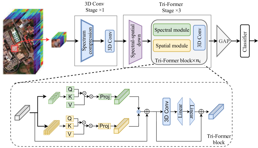
Figure 1: Architecture of proposed Tri-Former.

III-B Proposed Tri-Former

The architecture of the proposed Tri-Former is depicted in Fig. 1. The main body of the framework consists of four stages, including one stage of 3D convolution architecture and three stages of ViT blocks, as shown in the top half of Fig. 1. To be more specific, stage one comprises a spectrum compression module and a 3D convolution block. The subsequent three stages are constructed with the proposed Tri-Former modules. Each stage begins with a spectral-spatial downsample layer, followed by $n_{i}$ Tri-Former modules. After processing through the main body, the learned features are converted into feature vectors using global average pooling (GAP). Finally, a classifier is employed to generate the final prediction label.

The design of the main body follows two major principles:

• Early convolution principle. Indeed, it is possible to create a pure ViT network by employing the proposed Tri-Former block for all four stages. However, we refrain from adopting this structure due to the relatively low stability of pure ViT architectures. According to our experiments, we find that incorporating convolutions at the initial stage of the network enhances its stability and contributes to achieving better overall performance. This observation aligns with recent research findings [44, 45], which also advocate for the combination of convolutions with the ViT architecture to improve stability and performance. Therefore, we opt for a hybrid approach that leverages the advantages of both ViT and ConvNet components to build a more robust and efficient network.

• Hierarchical architecture principle. The entire network incorporates four downsampling layers, which are responsible for compressing the features along both the spectral and spatial dimensions. This hierarchical architecture primarily aims to reduce computation cost while maintaining effective information representation. At the beginning of each stage, spectrum compression or spectral-spatial downsample layers are employed to compress the input features, resulting in a more compact feature cube. Following a classical design strategy, the widths of the four stages are progressively doubled from stage to stage. In this context, we have set the width of the first stage to 32 as the starting point for subsequent widening. This design choice enables the network to efficiently process and extract relevant information in a computationally efficient manner.

The details of the proposed Tri-Former is shown in the bottom half of Fig. 1. Tri-Former has three main parts, spectral module, spatial module and 3D convolution module, which is why we call it triplet-structured. The spectral module is responsible for collecting information from different spectrum bands. The spatial module is in charge of collecting information from different space locations. We add a 3D convolution layer in before the two linear layers to enforce 3D structure information.

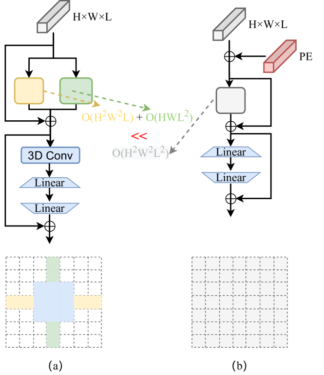
Figure 2: Comparison between proposed Tri-Former block and vanilla ViT block. (a) Proposed Tri-Former block; (b) Vanilla ViT block.

Compared with the vanilla ViT, we introduced two modifications:

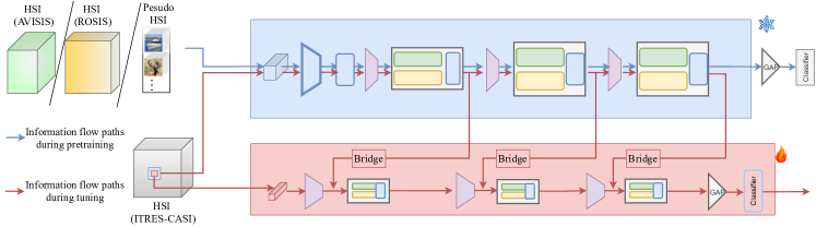
Figure 3: Architecture of proposed SDT. Blue part is basic model, where big patch and heavy Tri-Former are adopted. Red part is an auxiliary branch, where small patch and tiny Tri-Former are used. Bridges are point wise convolutions, which are responsible for adapting feature dimensions.

• Spectral-spatial parallel architecture. The adoption of such a design primarily stems from two reasons. Firstly, according to the first fundamental principle summarized in Section II, subsection A, both spectral and spatial information are important. Differing from previous works [20], which only apply self attention mechanism along spectral or spatial dimension only. Secondly, instead of directly applying self attention on three dimensions (two spatial dimensions and one spectral dimension), spectral and spatial dimensions are separately processed for reducing computation cost. The computation complexity of the vanilla ViT is quantic complex regarding to the length of the input sequence. In 3D architecture HSI, this issue is more serious. As shown in Fig 2, for a input with size of $H\times W\times L$, the computation complexity is $O(H^{2}W^{2}L^{2})$. In the spectral-spatial parallel architecture we have devised, the computational complexity becomes $O(H^{2}W^{2}L)+O(HWL^{2})$. In practical experiments, the value of $L$ is relatively large, making $O(H^{2}W^{2}L)+O(HWL^{2})$ significantly smaller than $O(H^{2}W^{2}L^{2})$. Therefore, our designed block markedly reduces computational load, rendering the entire architecture more lightweight and adaptable.

• 3D convolution enhanced channel mixer. Following fundamental principle two, 3D convolution is still heavily used in Tri-Former. In the channel mixer part, a 3D convolution is employed. Such a design has two advantages: 1) this additional 3D convolution contributes to stabilize the optimization process of the transformer block; 2) it enhances the structure information (position information) and obviates the necessity to rely on position embedding in the original ViT. Overall, the introduction of 3D convolutions results in a more flexible and stable module optimization tailored to HSI.

It is worth noting that the aforementioned two enhancements have significantly impacted the receptive field of the entire model. The receptive field in the proposed block excludes certain irrelevant elements within its scope, consequently strengthening the attention on pixels with close relationships. We illustrate the receptive fields of both our proposed module and the traditional transformer in Fig. 2 using two-dimensional features as an example. From Fig. 2(b), it is evident that the receptive field of the transitional structure is a square region. But as in Fig. 2(a), our design considers pixels that share the same row, column, or spatially adjacent positions with the central pixel. The self-attention operation in the ViT architecture achieves information fusion by computing approximate similarities between each pair of pixels. However, when a pixel is relatively distant from the central pixel, it may not effectively contribute to extracting information from the central pixel. Thus, retaining such distant pixels within the receptive field may indeed introduce noise. Therefore, the receptive field of our proposed module retains only the most crucially related pixels, while excluding irrelevant interference pixels, resulting in a more efficient mechanism.

III-C Proposed Single-Direction Tuning

Due to the high costs associated with HSI acquisition and annotation, how to achieve promising performance with very limited samples is a meaningful and open problem. Aiming to this problem, we proposed a single-direction tuning (SDT) strategy. As illustrated in Fig. 3, the function of SDT is like a bridge, bridging the gaps between HSI datasets captured by different sensors and datasets from different modalities. Utilizing the principles of SDT, we have the capability to enhance performance on novel HSI datasets with limited samples by leveraging either pre-existing labeled HSI datasets or RGB datasets.

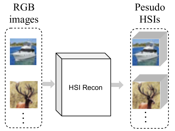
Figure 4: Framework of generating pseudo HSIs data from RGB images.

The process of SDT has two sequential stages:

• Firstly, pretraining the basic model with homogeneous and heterogeneous hyperspectral data, even RGB data, as illustrated in the blue part of Fig. 3. Here, to mitigate the modal disparities, we first employ the approach [46] to create the 32-channel pseudo-HSI data from RGB data and then use these pseudo-HSIs to perform pretraining, as depicted in Fig. 4. These generated images possess certain hyperspectral characteristics while harnessing the advantages of extensive natural image data. Experimental results in Section IV, subsection F demonstrate that the SDT can also benefit from RGB data.

• Secondly, a tiny auxiliary branch is tuned and applied to new HSI datasets, as presented in the red part of Fig. 3. To reduce the overhead associated with the auxiliary branch, we choose smaller patches, shallower architectures, and narrower modules. Unlike previous fine-tuning methods [47, 48, 49], where the base model remains frozen during tuning, we employ an asynchronous cold-hot gradient update strategy, where the basic model is updated slowly. Additionally, the bridge we establish between the base model and the auxiliary branch is unidirectional.

In terms of design, SDT has three notable aspects that guarantee its effective functioning in our scenario. To elaborate further:

• Parallel architecture. This design is inspired by the core idea of visual-prompt tuning (VPT) [47]. In VPT, learnable prompt and a new head are added and continuously updated to suit new tasks. The integration of new prompt and head incurs minimal additional costs. In our SDT approach, a tiny auxiliary branch is introduced and updated to adapt to the new datasets. This modification arises from the acknowledgment that distinct Hyperspectral Imaging (HSI) datasets exhibit more pronounced variations when compared to the disparities between diverse RGB datasets. Incorporating only a limited number of new learnable prompts has been demonstrated to be insufficient for effectively bridging this gap. Such a parallel architecture offers two distinct advantages. Firstly, during the tuning process, detaching the foundational model from gradient updating becomes effortless, enabling a more controlled adjustment. This adjustment aligns perfectly with the requirements for fine-tuning the ViT model for HSI classification. Secondly, the architectural design of the auxiliary branch is more flexible.

• Asynchronous cold-hot gradient update strategy. From our experiments, we find that completely freezing the foundational model as what do in RGB image processing and NLP fields [47, 48] does not work well in HSI classification. We speculate that this phenomenon arises due to the significant disparities among different HSI datasets. Therefore, a more suitable approach involves gradually fine-tuning the foundational model, allowing it to adjust appropriately and accommodate new data. Therefore, we propose an asynchronous cold-hot gradient update strategy, where basic model is updated slowly (cold) and the auxiliary branch is updated quickly (hot).

• Single-direction. During the tuning process, our goal is to ensure that the foundational model is appropriately adjusted to incorporate new data while maintaining its capacity for representation learning. To achieve this, we construct a single-direction bridge, which prevents the foundational model from being excessively influenced by gradients originating from the auxiliary branch.

To sum up, the design of SDT adheres to the third foundational principle, which aligns the classification framework with the intrinsic attributes of hyperspectral imagery. In this context, our focus primarily centers on the inherent diversity of physical traits displayed by various hyperspectral image datasets. Moving forward, we proceed to compare the proposed SDT approach with alternative fine-tuning and tuning strategies, analysing them from the perspective of gradient updates. Through this comparison, we aim to clarify the reasoning behind the SDT in our specific scenario.

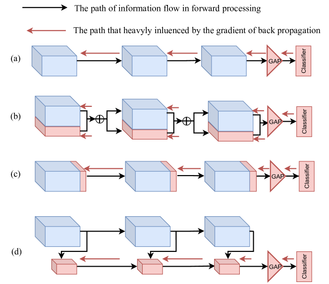
Figure 5: Comparison of different tuning architectures.

Comparative analysis in Fig. 5 highlights the distinctive nature of our proposed SDT strategy against prevailing methodologies. In traditional fine-tuning method, as depicted in Fig. 5(a), each feature undergoes significant gradient adjustments throughout the fine-tuning process. Fig. 5(b) illustrates the workflow of the LORA strategy, which introduces trainable rank decomposition matrices into each layer of the Transformer architecture, requiring matrix adjustments during tuning. Adaptor approaches, shown in Fig. 5(c), introduce new feature layers after each block, tuning block-specific features. Our proposed SDT is depicted in Fig. 5(d). As different HSI datasets have different physical attributes, completely freezing the basic model can not guarantee that the new model is suitable for the new dataset, which impacts the final performance. Therefore, updating the basic model is necessary. Nevertheless, if we adhere to the architecture of techniques like fine-tuning, Clip-adaptor, and LORA, the foundational model becomes significantly affected by the newly introduced modules. This outcome effectively nullifies the benefits acquired through pre-training, even when employing a cold-hot gradient update strategy. The corresponding experiments are presented in Section IV, subsection E.

IV Experiments

TABLE I: Sample distribution information of Datasets

Indian Pines			Pavia University		Houston University
Class	Land Cover Type	No.of Samples	Land Cover Type	No.of Samples	Land Cover Type	No.of Samples
1	Alfalfa	46	Asphalt	6631	Healthy Grass	1251
2	Corn-notill	1428	Meadows	18649	Stressed Grass	1254
3	Corn-mintill	830	Gravel	2099	Synthetic Grass	697
4	Corn	237	Trees	3064	Trees	1244
5	Grass-pasture	483	Painted Metal Sheets	1345	Soil	1242
6	Grass-trees	730	Bare Soil	5029	Water	325
7	Grass-pasture-mowed	28	Bitumen	1330	Residential	1268
8	Hay-windrowed	478	Self-Blocking Bricks	3682	Commercial	1244
9	Oats	20	Shadows	947	Road	1252
10	Soybean-notill	972	-	-	Highway	1227
11	Soybean-mintill	2455	-	-	Railway	1235
12	Soybean-clean	593	-	-	Parking Lot 1	1233
13	Wheat	205	-	-	Parking Lot 2	469
14	Woods	1265	-	-	Tennis Court	428
15	Buildings-Grass-Trees-Drives	386	-	-	Running Track	660
16	Stone-Steel-Towers	93	-	-	-	-
	Total	10249	Total	42776	Total	15029

IV-A Data Description

The three HSI datasets used in our experiments are Indian Pines, Pavia University, and Houston University. The sample distribution information is listed in Table I

Indian Pines dataset was acquired by the Airborne Visible/Infrared Imaging Spectrometer (AVIRIS) sensor during a flight campaign over the Indian Pines agricultural site in Indiana, USA. The Indian Pines dataset consists of a hyperspectral image with a high spectral resolution, capturing information in 224 contiguous spectral bands covering the wavelength range from 0.4 µm to 2.5 µm. The spatial resolution of the dataset is 145×145 pixels, making it relatively small compared to some other hyperspectral datasets. The primary objective of the Indian Pines dataset is to classify the various land-cover objects present in the agricultural area, which includes crops, bare soil, and different types of vegetation. The dataset contains 16 different land-cover classes in total.

Pavia University dataset was collected by the Reflective Optics System Imaging Spectrometer (ROSIS) sensor during a flight campaign over Pavia, a city in northern Italy. The dataset consists of a hyperspectral image with a high spectral resolution and geometric resolution of 1.3 meters. It captures information in 103 contiguous spectral bands covering the wavelength range from 0.43 µm to 0.86 µm. The spatial resolution of the Pavia University dataset is 610×340 pixels, making it of moderate size. The dataset contains 9 land-cover classes, representing various ground objects and materials present in the urban and agricultural regions of Pavia. The main objective of the Pavia University dataset is to classify the different land-cover classes present in the scene, which includes urban areas, vegetation, soil, and other materials.

Houston University dataset was captured by the ITRES-CASI 1500 hyperspectral imager over the University of Houston campus and the neighboring urban area in June 2012. The dataset comprises a hyperspectral image with a high spectral resolution, covering 144 contiguous spectral bands that span the wavelength range from 0.36 µm to 1.05 µm. With a spatial resolution of 349×1905 pixels, the Houston University dataset is relatively large, providing a detailed representation of the urban and suburban regions in the vicinity of the university. Houston University dataset consists of 349 × 1905 pixels. The dataset encompasses 15 distinct land-cover classes, including urban structures, roads, vegetation, water bodies, and other land-use categories typically encountered in urban environments.

IV-B Experiment Design

The experimental setup encompasses two comparative segments for classification evaluation. The first part involves basic model comparison experiments, while the second focuses on comparing various tuning strategies.

In basic model comparison part, we partition each target HSI dataset into two subsets: the training set and test set. We randomly extract 150 samples from each category as test samples and take the rest as the training samples in Pavia University dataset and Houston University. For the Indian Pines dataset, we sample a small number of pixels from classes with scarce samples to ensure a more balanced representation for the experiments. Concretely, we randomly select 10 samples from each of the following six classes: Alfalfa (class 1), Grass/trees (class 5), Grass/pasture-mowed (class 7), Oats (class 9), Buildings-grass-trees (class 15), and Stone-steel towers (class 16). For the remaining classes, we sample 150 pixels from each class. In this Section IV, subsection D, we compare our proposed Tri-Former model with other state-of-the-art algorithms.

In the context of tuning strategies comparison part in Section IV, subsection E, we compare the proposed SDT approach with other popular tuning methods on hyperspectral data collected from different sensors. Our experiments involve data from two source sensors: Salinas (captured by AVIRIS) and Pavia Center (captured by ROSIS). For the model trained on the data collected by each source sensor, we fine-tune it on the target data collected from another sensor with a limited number of samples. We design different experimental groups, each containing 25, 50, and 75 labeled pixels per class, respectively. Furthermore, in Section IV, subsection E, we evaluate the ability of the proposed method on tuning model pretrained on RGB images for application on HSI datsets.

Through comprehensive and systematic experiments, we demonstrate the effectiveness of our proposed method in addressing hyperspectral image classification. To ensure the fairness and stability of the comparison, we repeat each experiment five times and take the average values as the final results.

IV-C Implementation Details and Evaluation Metrics

Implementation details: The optimization of proposed method consists of two stages. The entire learning process is conducted on the server with 8 NVIDIA 3090 GPUs. During Training, the training samples are cropped as 27x27 spatial resolution patches, with a batch size of 96 on all three training dataset. We utilize the AdamW optimizer with a learning rate and weight decay value of $1\times 10^{-3}$ and $1\times 10^{-5}$, respectively. The learning rate decays from $1\times 10^{-3}$ to $1\times 10^{-6}$ following the cosine scheduler. The warming-up stage comprises 5 epochs and all the models are trained for 300 epochs. To further tune the final network, we crop patches with spatial resolutions of 13x13 and 27x27, which are fed into the auxiliary branch and main branch, respectively. Batch sizes are set to 12 for all datasets during tuning.

IV-D Comparison with state-of-the-art methods

In this section, we conduct a comparative analysis of our proposed Tri-Former against four ConvNet-based and Transformer-based HSI classification methods. The comparison is based on official code implementations of these methods: 3D-CNN, LWNet, SpectralFormer and SSFTT. The experimental results are presented in Tables II to  IV, and the visual comparisons are shown in Figs. 6 to 8.

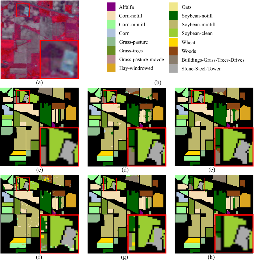
Figure 6: Results on Indian Pines. (a) Composite color map; (b) Ground truth; (c) 3D-CNN; (d) LWNet; (e) SpectralFormer; (f) SSFTT; (g) Tri-Former.

TABLE II: Comparison Experimental Results on Indian Pines Using 150 Training Samples Each Class

Models	3D-CNN	LWNet	SpectralFormer	SSFTT	Tri-Former
1	91.67	97.22	77.78	100.00	94.29
2	94.84	96.01	90.06	94.99	99.37
3	99.12	98.82	94.26	99.12	98.09
4	100.00	100.00	98.85	100.00	100.00
5	100.00	100.00	99.10	100.00	92.18
6	100.00	99.83	98.97	99.83	99.66
7	100.00	100.00	94.44	100.00	94.44
8	100.00	100.00	100.00	100.00	100.00
9	100.00	100.00	100.00	100.00	100.00
10	99.39	100.00	96.35	99.51	99.27
11	92.41	98.39	90.54	95.05	98.79
12	98.42	99.77	96.61	99.55	95.26
13	100.00	100.00	100.00	100.00	100.00
14	98.92	99.91	98.92	98.82	99.91
15	66.49	70.74	68.35	89.63	96.28
16	90.36	91.57	84.33	83.13	95.18
OA	95.23	97.46	93.08	97.12	98.44
AA	95.73	97.02	93.04	97.54	97.67
K	94.47	97.05	91.97	96.66	98.19

TABLE III: Comparison Experimental Results on Pavia University Using 150 Training Samples Each Class

Models	3D-CNN	LWNet	SpectralFormer	SSFTT	Tri-Former
1	91.09	96.06	83.13	94.69	99.86
2	92.05	95.69	92.83	98.74	99.99
3	92.45	95.95	89.34	98.50	100.00
4	98.55	98.68	97.60	95.05	98.83
5	99.52	99.92	100.00	97.43	100
6	93.14	98.09	90.32	99.96	99.98
7	97.48	99.76	96.99	100.00	99.92
8	95.20	99.11	92.63	99.08	99.63
9	97.28	98.82	99.65	99.88	99.87
OA	93.26	96.86	91.65	98.03	99.85
AA	95.20	98.01	93.61	98.15	99.79
K	91.13	95.84	89.00	97.38	99.80

The performance on the Indian Pines is listed in Table II. The corresponding visual comparison results are shown in Fig 6. Table II shows that the proposed Tri-Former achieves the highest OA of 98.44%, outperforming other ConvNet-based HSI classification methods like 3D-CNN (95.23%), LWNet (97.46%) and SpectralFormer (93.08%), and SSFTT (97.12%). Note that benefiting from the superior ability to represent deep semantic features, the SSFTT also outperforms several current state-of-the-art methods. The proposed Tri-Former further improved the OA metric of SSFTT by 1.32%, demonstrating its remarkable capability to accurately classify hyperspectral images in this challenging dataset. Fig 6 is the corresponding visual results. At the top, a color-composite image is presented, accompanied by color codes that represent different types of ground objects. The bottom-right corner features a magnified view, aimed at providing a clearer comparison of the classification performance of different methods. From Fig 6, we can see that all methods exhibit varying degrees of misclassification. Our proposed Tri-Former demonstrates the least amount of misclassification, approaching the ground truth closely.

Here, the performance of SpectralFormer still lags behind certain ConvNet-based methods. This phenomenon supports our statement that pure ViT is more data-hungry than ConvNet. SpectralFormer works well when the training samples are sufficient. But, it is not suit for the case where training samples are very limited. The performance of the SSFTT model is notably strong, surpassing the effectiveness of previous approaches. The incorporation of convolutional operations within the structure of SSFTT contributes to this improvement. This linear improvement further substantiates some of the points mentioned in our method section. Introducing convolutional operations to construct hybrid transformer models for processing HSI is a more suitable approach.

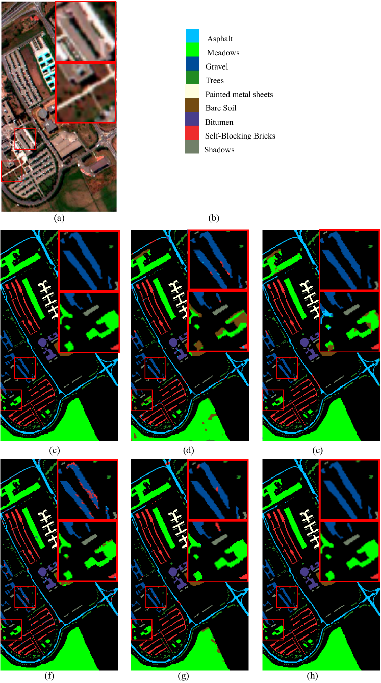
Figure 7: Results on Paiva University. (a) Composite color map; (b) Ground truth; (c) 3D-CNN; (d) LWNet; (e) SpectralFormer; (f) SSFTT; (g) Tri-Former.

Similar trends are also demonstrated in the experiments conducted on the Pavia University and Houston University datasets. When evaluated on the Pavia University dataset, our algorithm surpasses the state-of-the-art method SSFTT, achieving remarkable improvements in key evaluation metrics. Specifically, we observe substantial enhancements in Overall Accuracy (OA), Average Accuracy (AA), and Kappa (K) coefficient by 1.82%, 1.64%, and 2.42%, respectively. On the Houston University dataset, where the potential for performance improvement is considerably limited, our Tri-Former still manages to achieve the best performance among all methods compared. Fig 7 and Fig 8 are the corresponding visual comparison results. On these two datasets, especially on Pavia University dataset, proposed Tri-Former produces classification result maps that closely resemble the groundtruth.

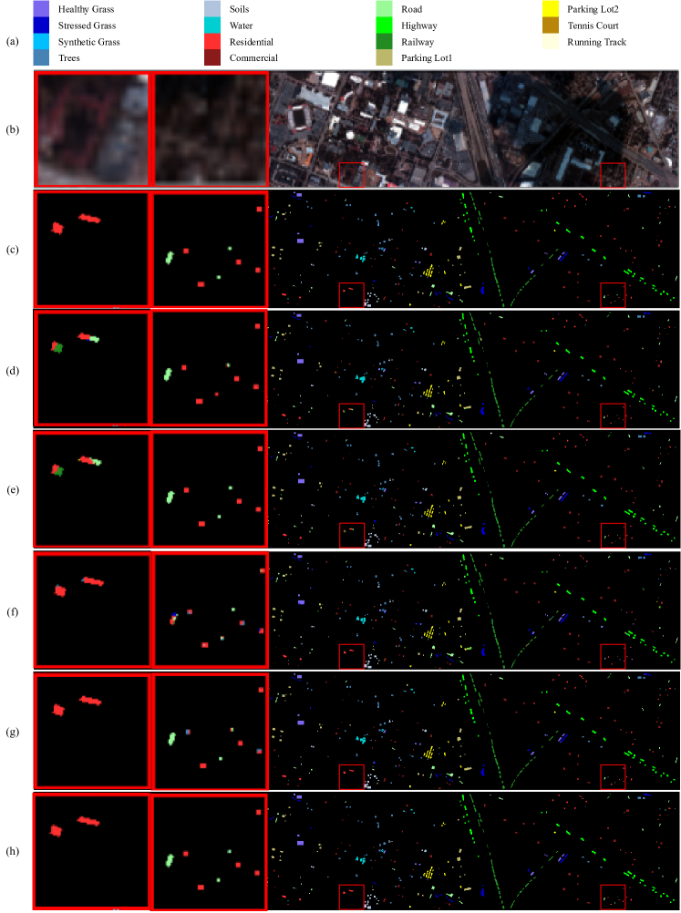
Figure 8: Results on Houston University. (a) Composite color map; (b) Ground truth; (c) 3D-CNN; (d) LWNet; (e) SpectralFormer; (f) SSFTT; (g) Tri-Former.

TABLE IV: Comparison Experimental Results on Houston University Using 150 Training Samples Each Class

Models	3D-CNN	LWNet	SpectralFormer	SSFTT	Tri-Former
1	96.64	98.64	96.00	98.00	98.73
2	95.20	99.01	89.31	97.10	98.28
3	99.82	100.00	99.09	99.09	100.00
4	97.62	99.54	86.47	97.90	96.80
5	99.45	100.00	95.88	100.00	100.00
6	100.00	100.00	86.86	100.00	100.00
7	91.68	96.06	73.23	98.66	98.66
8	94.70	96.71	85.56	97.62	98.90
9	96.82	97.19	85.57	99.82	98.37
10	98.33	99.44	91.55	100.00	99.91
11	97.05	100.00	92.35	100.00	98.71
12	96.12	98.25	86.98	96.21	99.45
13	95.61	100.00	82.45	99.37	100.00
14	100.00	100.00	100.00	100.00	100.00
15	100.00	100.00	97.65	100.00	99.61
OA	96.58	98.70	89.19	98.69	99.02
AA	97.14	98.99	89.93	98.92	99.17
K	96.29	98.59	88.28	98.57	98.85

During the network architecture design process, we adhered to the design principles outlined in the related work. Additionally, we took some guidelines from the recent developments in RGB image processing into account when designing the network. Finally, by merging these considerations with the characteristics unique to hyperspectral images, we formulated the Tri-Former architecture. These guidelines jointly ensure that the Tri-Former exhibits strong performance.

IV-E Comparison with other architecture tuning methods

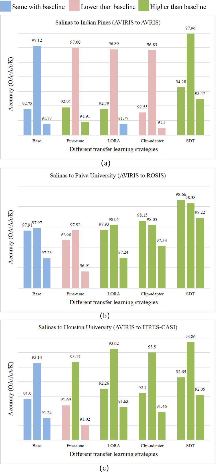
Figure 9: Comparison of different architecture tuning strategies.

For evaluating the effectiveness of our proposed SDT strategy, we conducted a comprehensive comparison with several representative architecture tuning methods. The comparison methods involved in the evaluation are as follows: Fine-tune (adopted in LWNet and Two-CNN for ConvNet methods), LORA and Clip-adapter (for transformer methods).

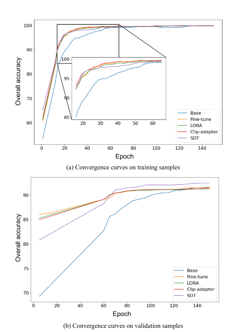
Figure 10: Convergence curves of different architecture tuning strategies.

In this experiment, the basic model is first pretrained on the Salinas dataset acquired through the AVRIS sensor. Then, the model is fine-tuned with various strategies on three distinct target datasets captured by different sensors: AVRIS, ROSIS, and ITRES-CASI. Within the tuning stage, each class is provided with 50 training samples. The experimental results are consolidated in Fig 9, where the x-axis denotes the employed methods and the y-axis depicts the evaluation metric. According to the comparison, we can draw four conclusions:

• Conventional fine-tuning strategy tailored for ConvNets proves ineffective in our scenario. As shown in Fig 5, the Fine-tune strategy not only fails to yield any improvement but also negatively affects the final results. We hypothesize that this lack of improvement can be attributed to the fundamental differences between the information learned by ConvNets and Transformer methods. ConvNets learn a set of filter parameters from the training data. The process of feature extraction in ConvNets is static. Differing from this, Transformer architectures learn relationships between pixels, capturing global dependencies in the data. Transformer is a data-driven model and its feature extraction process is dynamic, which is more sensitive to the difference between dataset used for pretraining and the new target dataset. Unfortunately, there are obvious differences among HSI datasets, which consequently hinder the effectiveness of fine-tuning.

  

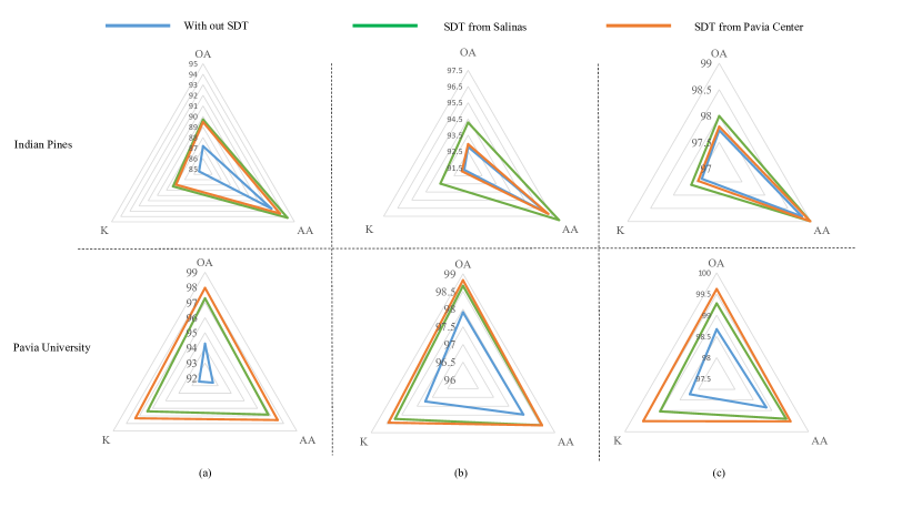
  Figure 11: Experiments on homogeneous and heterogeneous HSI datasets. (a) 25 training samples per class; (b) 50 training samples per class; (c) 75 training samples per class.

• Architecture tuning does have an impact on training effectiveness. To conduct a comprehensive analysis of different tuning strategies, we have plotted their respective convergence curves. As shown in Fig 10, compared with baseline, each tuning strategy exhibits a distinct convergence curve. Specifically, each tuning model achieves very high accuracy at beginning. The accuracy of training the base model (in blue line) gradually catches up with the accuracy curves of Fine-tune, Clip-adapter, and LORA. However, it still lags behind the convergence curve of SDT. We attribute this phenomenon mainly to the following reason. At the beginning of training, the baseline model starts with random initialization and lacks any feature extraction capability. Meanwhile, the tuned models have already learned feature extraction capabilities from heterogeneous data, allowing them to exhibit some effectiveness from the outset. During the training process, the baseline model benefits from the optimization on the new data, while tuned models may suffer from the conflicts gradually arising from the heterogeneous data. This dynamic change results in the baseline catching up with, and in some cases, surpassing the tuned models.

• Architecture tuning strategies proposed for transformer model have a certain role in our specific scenario as well. LORA and Clip-adaptor are specifically designed for transformer-based algorithms, and they do achieve higher classification accuracy compared to fine-tuning methods tailored for CNNs. However, despite their overall performance advantage, these two fine-tuning methods still exhibit negative effects in certain experiments. We speculate the reason is that the pretrained basic model is heavily influenced during tuning stage. When the adaptor introduces significant changes to the main network during fine-tuning, the fine-tuned model may lose some of the informative features learned during pre-training. As a result, the performance of LORA and Clip-adaptor could be negatively impacted in certain scenarios, particularly when there are a lot of differences between the pre-training and fine-tuning datasets. Significant updating of the main network’s parameters may disrupt the underlying spectral-spatial patterns captured during pre-training, leading to a drop in classification accuracy.

• Proposed SDT works well. Serving as a bridge, SDT ensures that the fine-tuning process adapts the model to the target dataset while preserving the generic spectral-spatial representations learned during pre-training. This approach enables SDT to capitalize on architecture tuning effectively, even when faced with diverse datasets, and contributes to its superior performance in various experimental scenarios.

IV-F Experiments on homogeneous and heterogeneous HSI datasets

To further validate the effectiveness of our method and investigate the influence of homogeneity and heterogeneity on tuning experiments, we conducted two sets of experiments on Indian pines, Salinas, Pavia University and Pavia Center. The first two datasets are homogeneous datasets captured by AVRIS. The last two datasets are homogeneous datasets captured by ROSIS. In the first experiment set, the foundational model was pretrained on the Salinas dataset. Subsequently, it was fine-tuned on the Indian Pines and Pavia University datasets respectively, under three distinct configurations: 25, 50, and 75 training samples settings.

The experimental results are depicted in the form of radar charts in Figure 11, from which we can see that:

• SDT consistently enhances performance across all settings. Whether in a homogenous or heterogeneous scenario, employing SDT consistently leads to a significant improvement in accuracy, which once again proves the effectiveness of our SDT strategy.

• Transfer between homogenous datasets holds more advantages compared to transfer between heterogeneous datasets. In LWNet [14], the transfer experiments reveal that regardless of whether it is a heterogeneous or homogeneous scenario, using Salinas pretraining yields better results compared to using Pavia pretraining. The reason behind this is that the Salinas dataset exhibits a greater diversity of samples, which contributes to the model’s enhanced generalization ability. Differring from this, in our case, the advantage of transferring between homogenous datasets is more pronounced. As shown in the experiments conducted on the Pavia University dataset, even though Pavia Center contains only ten classes and has less sample diversity compared to Salinas with 16 classes, the advantage of pretraining on Pavia Center becomes more obvious on Pavia University due to their homogeneity.

IV-G Effectiveness of sample diversity

Experiments in the last section verify the effectiveness of homogeneity. In this section, we pretain basic model on Salinas and Pavia Center, then tuning it on Houston Univeristy dataset to verify the effectiveness of sample diversity. For Houston University dataset, both Salinas and Paiva Center are heterogeneous datasets, but the Salinas has better sample diversity than Pavia Center. Similar with the last section, the experimental results are presented in the form of radar charts in Fig 12. From the results we can see that when all data is heterogeneous, training on a dataset with stronger diversity is more useful.

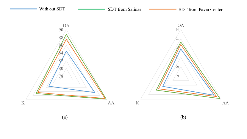
Figure 12: Prompt tuning experiments on Houston University. (a) 25 training samples per class; (b) 50 training samples per class.

TABLE V: Experimental Results of Cross Sensors Transfer Learning from RGB Data

Dataset	Indian pines		PaviaU		HoustonU
Sensor	RGB$\rightarrow$ AVIRIS		RGB$\rightarrow$ ROSIS		RGB $\rightarrow$ ITRES-CASI
Method	nSDT	SDT	nSDT	SDT	nSDT	SDT
OA	92.78	93.16	97.91	98.64	91.90	92.86
AA	97.12	97.38	97.97	98.64	93.14	93.85
K	91.77	92.19	97.23	98.19	91.24	92.27

IV-H Using SDT as a bridge between RGB datasets and HSI datasets

The experiments in the previous section reveal the importance of sample diversity. In terms of diversity, existing RGB datasets have strong diversity. The barrier between RGB and HSI datasets is that they are cross-modality datasets. In this section, we combine HSI reconstruction method and the proposed SDT to build a bridge to cross this barrier.

More specifically, we apply the trained HSI rescontruction model [46] to convert 3-channel RGB image to 32-channel pseudo-HSI image then use the pseudo-HSI to train the basic model. The RGB dataset used here is CIFAR-100. Experimental results are listed in Table V.

Interestingly, in this setup, SDT achieves results that are as good as, or even superior to, those obtained with homogenous data. Cross-modal experiments can be viewed as a further extension of cross-sensor experiments. At first glance, this experimental result seems contradictory to the previous results. We suspect that the main reason for this phenomenon is the strong sample diversity of the CIFAR-100 dataset, which offsets the effects of heterogeneous data to some extent. This is essential for remote sensing applications with expensive data collection costs.

Just as mentioned in our method, the proposed SDT serves as a bridge to address the modal differences between RGB datasets and HSI datasets. This is crucial, particularly considering the presence of datasets with even greater sample diversity in the realm of RGB datasets. The bridge allows us to make use of these datasets. Additionally, to enhance the HSI classification performance, larger models are required. Larger labeled datasets are necessary for training these larger models. SDT provides a way to effectively leverage existing RGB datasets to enhance the accuracy of hyperspectral image classification.

V Conclusion

In this paper, we have presented the Triplet-structured Transformer (Tri-Former) model, a strategic response to challenges in adopting Vision Transformer (ViT) models for Hyperspectral Image (HSI) classification. By integrating parallel attention modules and a 3D convolution-based channel mixer, Tri-Former optimizes computational efficiency while enhancing model stability. Furthermore, to more effectively diminish the demand for an extensive quantity of training samples, we introduce Single-Direction Tuning (SDT) strategy. Acting as a bridge, SDT enables us to capitalize on both pre-existing labeled HSI datasets and even RGB datasets, thereby enhancing the performance on new HSI datasets with constrained sample sizes. Extensive experiments across diverse HSI datasets and sensors verified the proposed Tri-Former. Homologous, heterologous, and cross-modal tuning experiments are conducted to validate the performance of the proposed SDT.

References

- [1] M. J. Khan, H. S. Khan, A. Yousaf, K. Khurshid, and A. Abbas, “Modern trends in hyperspectral image analysis: A review,” IEEE Access, vol. 6, pp. 14 118–14 129, 2018.
- [2] Y. Gu, J. Chanussot, X. Jia, and J. A. Benediktsson, “Multiple kernel learning for hyperspectral image classification: A review,” IEEE Transactions on Geoscience and Remote Sensing, vol. 55, no. 11, pp. 6547–6565, 2017.
- [3] T. A. Carrino, A. P. Crósta, C. L. B. Toledo, and A. M. Silva, “Hyperspectral remote sensing applied to mineral exploration in southern peru: A multiple data integration approach in the chapi chiara gold prospect,” International journal of applied earth observation and geoinformation, vol. 64, pp. 287–300, 2018.
- [4] J. Behmann, J. Steinrücken, and L. Plümer, “Detection of early plant stress responses in hyperspectral images,” ISPRS Journal of Photogrammetry and Remote Sensing, vol. 93, pp. 98–111, 2014.
- [5] J. Transon, R. d’Andrimont, A. Maugnard, and P. Defourny, “Survey of hyperspectral earth observation applications from space in the sentinel-2 context,” Remote Sensing, vol. 10, no. 2, p. 157, 2018.
- [6] Z. Lin, Y. Chen, X. Zhao, and G. Wang, “Spectral-spatial classification of hyperspectral image using autoencoders,” in 2013 9th International Conference on Information, Communications & Signal Processing. IEEE, 2013, pp. 1–5.
- [7] Y. Chen, Z. Lin, X. Zhao, G. Wang, and Y. Gu, “Deep learning-based classification of hyperspectral data,” IEEE J. Sel. Topics Appl. Earch Observ. Remote Sens., vol. 7, no. 6, pp. 2094–2107, Jun. 2014.
- [8] Y. Chen, X. Zhao, and X. Jia, “Spectral–spatial classification of hyperspectral data based on deep belief network,” IEEE J. Sel. Topics Appl. Earch Observ. Remote Sens., vol. 8, no. 6, pp. 2381–2392, Jun. 2015.
- [9] H. Zhang, Y. Li, Y. Zhang, and Q. Shen, “Spectral-spatial classification of hyperspectral imagery using a dual-channel convolutional neural network,” Remote sensing letters, vol. 8, no. 5, pp. 438–447, 2017.
- [10] Y. Li, H. Zhang, and Q. Shen, “Spectral–spatial classification of hyperspectral imagery with 3d convolutional neural network,” Remote Sensing, vol. 9, no. 1, p. 67, 2017.
- [11] Y. Chen, H. Jiang, C. Li, X. Jia, and P. Ghamisi, “Deep feature extraction and classification of hyperspectral images based on convolutional neural networks,” IEEE Trans. Geosci. Remote Sens., vol. 54, no. 10, pp. 6232–6251, Oct. 2016.
- [12] H. Zhang, C. Gong, Y. Bai, Z. Bai, and Y. Li, “3-d-anas: 3-d asymmetric neural architecture search for fast hyperspectral image classification,” IEEE Transactions on Geoscience and Remote Sensing, vol. 60, pp. 1–19, 2021.
- [13] H. Liu, K. Simonyan, and Y. Yang, “Darts: Differentiable architecture search,” in Proc. Int. Conf. Learn. Representations, 2019.
- [14] H. Zhang, Y. Li, Y. Jiang, P. Wang, and C. Shen, “Hyperspectral classification based on lightweight 3-d-cnn with transfer learning,” IEEE Transactions on Geoence and Remote Sensing, vol. 57, no. 8, pp. 5813–5828, 2019.
- [15] J. Yang, Y.-Q. Zhao, and J. C.-W. Chan, “Learning and transferring deep joint spectral–spatial features for hyperspectral classification,” IEEE Trans. Geosci. Remote Sens., vol. 55, no. 8, pp. 4729–4742, Aug. 2017.
- [16] A. Vaswani, N. Shazeer, N. Parmar, J. Uszkoreit, L. Jones, A. N. Gomez, Ł. Kaiser, and I. Polosukhin, “Attention is all you need,” in Advances in neural information processing systems, 2017, pp. 5998–6008.
- [17] A. Dosovitskiy, L. Beyer, A. Kolesnikov, D. Weissenborn, X. Zhai, T. Unterthiner, M. Dehghani, M. Minderer, G. Heigold, S. Gelly et al., “An image is worth 16x16 words: Transformers for image recognition at scale,” arXiv preprint arXiv:2010.11929, 2020.
- [18] H. Touvron, M. Cord, M. Douze, F. Massa, A. Sablayrolles, and H. Jégou, “Training data-efficient image transformers & distillation through attention,” in International Conference on Machine Learning. PMLR, 2021, pp. 10 347–10 357.
- [19] Z. Liu, Y. Lin, Y. Cao, H. Hu, Y. Wei, Z. Zhang, S. Lin, and B. Guo, “Swin transformer: Hierarchical vision transformer using shifted windows,” arXiv preprint arXiv:2103.14030, 2021.
- [20] D. Hong, Z. Han, J. Yao, L. Gao, B. Zhang, A. Plaza, and J. Chanussot, “Spectralformer: Rethinking hyperspectral image classification with transformers,” IEEE Transactions on Geoscience and Remote Sensing, 2021.
- [21] L. Sun, G. Zhao, Y. Zheng, and Z. Wu, “Spectral–spatial feature tokenization transformer for hyperspectral image classification,” IEEE Transactions on Geoscience and Remote Sensing, vol. 60, pp. 1–14, 2022.
- [22] X. Xue, H. Zhang, B. Fang, Z. Bai, and Y. Li, “Grafting transformer on automatically designed convolutional neural network for hyperspectral image classification,” IEEE Transactions on Geoscience and Remote Sensing, vol. 60, pp. 1–16, 2022.
- [23] H. Zhang, W. Hu, and X. Wang, “Parc-net: Position aware circular convolution with merits from convnets and transformer,” in European Conference on Computer Vision. Springer, 2022, pp. 613–630.
- [24] ——, “Cabvit: Cross attention among blocks for vision transformer,” arXiv preprint arXiv:2211.07198, 2022.
- [25] P. Gao, S. Geng, R. Zhang, T. Ma, R. Fang, Y. Zhang, H. Li, and Y. Qiao, “Clip-adapter: Better vision-language models with feature adapters,” arXiv preprint arXiv:2110.04544, 2021.
- [26] E. J. Hu, Y. Shen, P. Wallis, Z. Allen-Zhu, Y. Li, S. Wang, L. Wang, and W. Chen, “LoRA: Low-rank adaptation of large language models,” in International Conference on Learning Representations, 2022. [Online]. Available: https://openreview.net/forum?id=nZeVKeeFYf9
- [27] Y.-L. Sung, J. Cho, and M. Bansal, “Lst: Ladder side-tuning for parameter and memory efficient transfer learning,” Advances in Neural Information Processing Systems, vol. 35, pp. 12 991–13 005, 2022.
- [28] A. Krizhevsky, I. Sutskever, and G. E. Hinton, “Imagenet classification with deep convolutional neural networks,” in Proc. Adv. Neural Inf. Process. Syst., 2012, pp. 1097–1105.
- [29] K. Simonyan and A. Zisserman, “Very deep convolutional networks for large-scale image recognition,” arXiv preprint arXiv:1409.1556, 2014.
- [30] C. Szegedy, S. Ioffe, V. Vanhoucke, and A. A. Alemi, “Inception-v4, inception-resnet and the impact of residual connections on learning.” in Proc. AAAI Conf. Intell., vol. 4, 2017, p. 12.
- [31] K. He, X. Zhang, S. Ren, and J. Sun, “Deep residual learning for image recognition,” in Proc. IEEE Conf. Comput. Vis. Pattern Recognit. (CVPR), Jun. 2016, pp. 770–778.
- [32] G. Huang, Z. Liu, K. Q. Weinberger, and L. van der Maaten, “Densely connected convolutional networks,” in Proc. IEEE Conf. Comput. Vis. Pattern Recognit. (CVPR), Jul. 2017, p. 3.
- [33] A. G. Howard, M. Zhu, B. Chen, D. Kalenichenko, W. Wang, T. Weyand, M. Andreetto, and H. Adam, “Mobilenets: Efficient convolutional neural networks for mobile vision applications,” arXiv preprint arXiv:1704.04861, 2017.
- [34] Z. Liu, H. Mao, C.-Y. Wu, C. Feichtenhofer, T. Darrell, and S. Xie, “A convnet for the 2020s,” Proceedings of the IEEE/CVF Conference on Computer Vision and Pattern Recognition (CVPR), 2022.
- [35] S. Mei, J. Ji, Q. Bi, J. Hou, Q. Du, and W. Li, “Integrating spectral and spatial information into deep convolutional neural networks for hyperspectral classification,” in Proc. IEEE Conf. Int. Geosci. Remote Sens. Symp (IGARSS),, Jul. 2016, pp. 5067–5070.
- [36] H. Zhang and Y. Li, “Spectral-spatial classification of hyperspectral imagery based on deep convolutional network,” in 2016 International Conference on Orange Technologies (ICOT). IEEE, 2016, pp. 44–47.
- [37] K. Makantasis, K. Karantzalos, A. Doulamis, and N. Doulamis, “Deep supervised learning for hyperspectral data classification through convolutional neural networks,” in Proc. IEEE Conf. Int. Geosci. Remote Sens. Symp (IGARSS),, Jul. 2015, pp. 4959–4962.
- [38] J. Yue, W. Zhao, S. Mao, and H. Liu, “Spectral–spatial classification of hyperspectral images using deep convolutional neural networks,” Remote Sensing Letters, vol. 6, no. 6, pp. 468–477, 2015.
- [39] Z. Zhong, J. Li, Z. Luo, and M. Chapman, “Spectral–spatial residual network for hyperspectral image classification: A 3-d deep learning framework,” IEEE Trans. Geosci. Remote Sens., vol. 56, no. 2, pp. 847–858, Feb. 2018.
- [40] X. He, Y. Chen, and Z. Lin, “Spatial-spectral transformer for hyperspectral image classification,” Remote Sensing, vol. 13, no. 3, p. 498, 2021.
- [41] Y. Qing, W. Liu, L. Feng, and W. Gao, “Improved transformer net for hyperspectral image classification,” Remote Sensing, vol. 13, no. 11, p. 2216, 2021.
- [42] S. J. Pan and Q. Yang, “A survey on transfer learning,” IEEE Transactions on knowledge and data engineering, vol. 22, no. 10, pp. 1345–1359, 2009.
- [43] W. Yu, C. Si, P. Zhou, M. Luo, Y. Zhou, J. Feng, S. Yan, and X. Wang, “Metaformer baselines for vision,” arXiv preprint arXiv:2210.13452, 2022.
- [44] B. Graham, A. El-Nouby, H. Touvron, P. Stock, A. Joulin, H. Jégou, and M. Douze, “Levit: a vision transformer in convnet’s clothing for faster inference,” arXiv preprint arXiv:2104.01136, 2021.
- [45] T. Xiao, M. Singh, E. Mintun, T. Darrell, P. Dollár, and R. Girshick, “Early convolutions help transformers see better,” Advances in neural information processing systems, vol. 34, pp. 30 392–30 400, 2021.
- [46] J. Li, S. Du, C. Wu, Y. Leng, R. Song, and Y. Li, “Drcr net: Dense residual channel re-calibration network with non-local purification for spectral super resolution,” in Proceedings of the IEEE/CVF conference on computer vision and pattern recognition, 2022, pp. 1259–1268.
- [47] M. Jia, L. Tang, B.-C. Chen, C. Cardie, S. Belongie, B. Hariharan, and S.-N. Lim, “Visual prompt tuning,” in European Conference on Computer Vision. Springer, 2022, pp. 709–727.
- [48] P. Liu, W. Yuan, J. Fu, Z. Jiang, H. Hayashi, and G. Neubig, “Pre-train, prompt, and predict: A systematic survey of prompting methods in natural language processing,” ACM Computing Surveys, vol. 55, no. 9, pp. 1–35, 2023.
- [49] X. Liu, K. Ji, Y. Fu, W. L. Tam, Z. Du, Z. Yang, and J. Tang, “P-tuning v2: Prompt tuning can be comparable to fine-tuning universally across scales and tasks,” arXiv preprint arXiv:2110.07602, 2021.