Foundations of continuous agent-based modelling frameworks for pedestrian dynamics and their implications

Abstract

This paper addresses the theoretical foundations of pedestrian models for crowd dynamics. While the topic gains momentum, widely different mathematical approaches are actually in use, even if we only consider continuous agent-based models. To clarify their underpinning, we first rephrase the common hierarchical decomposition into strategic, tactical, and operational levels and show the practical interest in preserving the continuity between the latter two levels by working with a floor field, rather than way-points. Turning to local navigation, we clarify how three archetypical approaches, namely, reactive models, anticipatory models based on the idea of times to collision (exemplified by the recently proposed ANDA model), and game theory, differ in their extrapolation of future trajectories, and insist on the oft-overlooked distinction between processes pertaining to decision-making and mechanical effects in dense settings. The differences are illustrated with a comparison of the numerical predictions of instances of these models in the simple scenario of head-on collision avoidance between agents, by varying the walking speed and the reaction times, notably.

1 Introduction

Many breakthroughs in modern science have hinged on a reshuffling of the mathematical framework in use. For instance, the ability of modern statistics to account for the regularities of human physical features or social events [1, 2] can hardly be dissociated from the mathematical handling of errors and uncertainties and the then-emerging theories of probabilities [3]; similarly, the theoretical revisitation of the foundations of economics by von Neumann and Morgenstern [4] has been instrumental for the progress of modern economics. Transportation Science has largely benefited from the advances in these two disciplines.

Presently, within the field of transportation, modelling pedestrian dynamics is a topic that gains more and more traction, due to both its practical relevance for crowd safety [5] and flow management, and its theoretical intricacy [6, 7]. But at the same time, little thought has been dedicated to the soundness of its conceptual foundations. In fact, one almost takes for granted that pedestrian models should retain the formal structure in place in the fields that inspired them.

Thus, models originating from the field of algorithmic robotics (or computer graphics) typically rely on the notion of velocity obstacles, i.e., the set of all velocities leading to a collision before a predefined time horizon [8, 9, 10], and the idea that the chosen velocity should not belong to this set. What matters most is to reach a target while avoiding collisions at all costs. In this sense, mathematical proofs are often given to guarantee the absence of collisions, at least in some regimes [11].

Shifting the emphasis from global maneuverability to individual choice, economists and econometricians have employed the structure of discrete-choice models to find which step is optimal [12] and adequately calibrate their model [13]; each agent then chooses to make a step which optimises a utility function depending on various factors. The idea of optimal steps was also taken up in the optimal-step model [14], from a more pragmatic standpoint.

By contrast, physicists have propounded a line of models that keep the formal structure of Newton’s second law and handle interactions between pedestrians in the same way as mechanical forces. This is the case for the celebrated social force model [15] and its countless extensions and variants [16, 17, 18]. Contacts and collisions between agents are then possible, particularly at high density, so that these models are frequently used to study evacuations; besides, they heavily (arguably, too heavily) rely on these contact forces to reproduce the collective flow of crowds [19]. Moussaid et al. insisted on the more heuristic nature at play in pedestrians’ decisions of motion, thereby slagging off the deterministic mechanical picture and putting forward simple heuristic rules instead, but they still resorted to a similar force-based equation in which the heuristic pseudo-force is summed with mechanical forces [20].

This study, which extends the short report in [21], is aimed at delving into the structural foundations of agent-based pedestrian models and clarifying their implications and differences. For that purpose, starting from a very broad perspective, Sec. 2 revisits the hierarchical decomposition into levels of description, showing that it can be misguiding to adhere to the distinction between the tactical level and the operational one too tightly. Then, we address the description of local navigation, and notably the interface between walking choices and mechanical contacts in dense settings, which is a singularity of crowds. After introducing three archetypal models for operational pedestrian dynamics in Sec. 3, we expose the differences in their numerical predictions in Sec. 4, with an emphasis on the simple scenario of head-on collision avoidance between agents.

2 A deep dive into the foundations of pedestrian agent-based models

2.1 Levels of description of pedestrian dynamics

In this section, we will enquire into the mathematical underpinning and conceptual relevance of splitting the modeller’s task into a strategic level (where do I want to go and when?), a tactical level (what route do I take to reach this goal?) and an operational level (how do I interact with the human and built environment locally, en route?), using the terminology of [22]; these levels are illustrated in Fig. 2.1. We will question the practical implications of the stark distinction that is made between the tactical and operational levels. This mathematical clarification will directly pave the way for different modelling options, differing by the extent to which the future is anticipated.

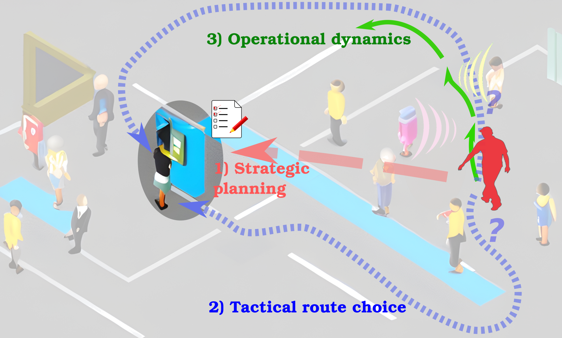
Figure 2.1: Schematic illustration of the different levels of description used in pedestrian modelling. Drawn using DeepAI.org.

First note that the foregoing levels of description may be coupled to some extent, but mostly rely on a coarse-grained vision of the lower levels. For instance, should I contemplate enjoying a day at the beach in a far-away island, my ultimate strategic decision may be influenced by my (tactical) knowledge of approximately how much it costs to fly there, in human, financial, and environmental terms. Once the strategic decision has been made, the agent will articulate the operational dynamics of local navigation with the route choice operated at the tactical level.

Thanks to its intuitive formulation and practical convenience, the foregoing decomposition has been widely applied. Nonetheless, to grasp its possible limitations, it is useful to make the definition sharper by phrasing it in mathematical terms, namely, in space-time $\Omega\times[0,T]$, where $\Omega\subset\mathbb{R}^{3}$ is the available geometric space and $[0,T]$ is the time window under consideration. The evolution of a crowd of $N$ agents is then represented by a set of $N$ trajectories $\boldsymbol{r}_{j}(t)$, for $j=1...N$ and $t\in[0,T]$. From this perspective, for each agent, a strategic choice consists in selecting a target region $\mathcal{T}_{j}$ in spacetime. The tactical choice then comes down to selecting a path route $\mathcal{R}_{j}$, i.e., a class of ‘equivalent’ trajectories that lead to the target $\mathcal{T}_{j}$, while navigation at the operational level will lead to the materialisation of only one trajectory $\boldsymbol{r}_{j}(t)$ in this class.

2.2 Selection of an optimal path

Once the strategic decision is made, agent $j$ has to select one route among all the possibilities $\mathcal{R}_{0}^{T}$ that match the agent’s goal. The selected route will be that which minimises a generalised cost $C_{j}$. Thus, the tactical choice can be regarded as an optimisation problem over a time window $[0,T]$, viz.,

$$\min_{\mathrm{routes}\ \mathcal{R}_{0}^{T}}C_{j}[\mathcal{R}_{0}^{T}]\ \ \ \tiny{\mathrm{[TACTICAL]}}$$ (1)

where the route cost is defined operationally as a minimum over all trajectories $\boldsymbol{r}_{j}$ belonging to that route,

$$C_{j}[\mathcal{R}_{0}^{T}]=\min_{\boldsymbol{r}_{j}\in\mathcal{R}_{0}^{T}}\int_{t}^{T}\underset{\text{running cost}}{\underbrace{c_{j}[\boldsymbol{r}_{j}(t^{\prime}),\boldsymbol{r}_{-j}(t^{\prime})]}}dt^{\prime}+\underset{\text{terminal cost}}{\underbrace{C_{j}^{T}[\boldsymbol{r}_{j}(T)]}}\ \ \ \tiny{\mathrm{[OPERATIONAL]}}.$$ (2)

Here, the running cost $c_{j}$ depends on agent $j$’s trajectory as well as the other agents’ trajectories $\boldsymbol{r}_{-j}=(\boldsymbol{r}_{1},...,\boldsymbol{r}_{j-1},\boldsymbol{r}_{j+1},...,\boldsymbol{r}_{N})$; the minimiser is the trajectory that is selected operationally. For concreteness, below, we will study simple running costs that just penalise large speeds and the spatial proximity to another agent with a repulsive potential.

Noteworthily, the tactical choice of Eq. 1 is fully entangled with the operational selection of Eq. 2. Adding to this complexity is the dependence of the individual costs $C_{j}$ on the other agents’ trajectories $\boldsymbol{r}_{-j}$. This is why the optimisation problem does not boil down to finding the local minimum of a function, but is a game [4] between different players, the agents, each intent on optimising their cost but unable to control the opponents’ decisions. In other words, the minimisation should be understood in the sense of a Nash equilibrium [23], i.e., agent $j$’s ‘optimal’ choice is conditioned on the fact that the the other agents’ trajectories $\boldsymbol{r}_{k}$, $k\neq j$, are also optimal for them.

Not only does this process make the model computationally complex, but one may also question its realism: Pedestrians are unable to accurately foresee the others’ trajectories; at best can they try to predict them, so that $\boldsymbol{r}_{-j}$ in Eq. 2 should be replaced by its prediction $\boldsymbol{\tilde{r}}_{-j}^{(j)}$ by agent $j$.

More pragmatically, one can treat future costs (say, beyond $\delta t$) using coarse-grained estimates, viz.,

$$C_{j}[\mathcal{R}_{0}^{T}] = C_{j}[\mathcal{R}_{0}^{\delta t}]+C_{j}[\mathcal{R}_{\delta t}^{T}]$$ (3)

$$\approx \min_{\boldsymbol{r}_{j}\in\mathcal{R}_{0}^{\delta t}}\int_{0}^{\delta t}c_{j}[\boldsymbol{r}_{j}(t^{\prime}),\boldsymbol{r}_{-j}(t^{\prime})]dt^{\prime}+\tilde{C}_{j}[\boldsymbol{r}_{j}(\delta t)],$$ (4)

where $\tilde{C}_{j}[\boldsymbol{r}_{j}(\delta t)]$ is an approximate assessment of the future cost beyond $\delta t$, that is assumed to depend only on the position $\boldsymbol{r}_{j}(\delta t)$ reached at that time. Note, in anticipation, that if $\delta t$ is small the trajectories can be considered linear, i.e., $\forall k\neq j,\ \boldsymbol{r}_{k}(t)\simeq\boldsymbol{r}_{k}(0)+\boldsymbol{v}_{k}(0)t$, so that the minimisation of Eq. 4 will ultimately reduce to a dynamical equation of motion: at each time $t$, each agent $j$ has to select an optimal velocity $\boldsymbol{v}_{j}^{\star}$.

Quite interestingly, these abstract considerations surreptitiously led to the substitution of the remaining cost $C_{j}[\mathcal{R}_{\delta t}^{T}]$ in the equation of motion by a floor field $\tilde{C}_{j}(\boldsymbol{r})$, i.e., a real-valued function $\Omega\to\mathbb{R}$ that quantifies how attractive a given location $\boldsymbol{r}$ is effectively, for every class of agents. In principle, it should exactly match the cost of the optimal route from $\boldsymbol{r}$ to the target location over the time window $[\delta t,T]$, but in practice this cost may be assessed roughly, notably in view of the proximity of $\boldsymbol{r}$ to the goal or via an Eikonal equation, traditionally used in ray tracing algorithms, in which the cost of walking through a given zone plays the role of an index of refraction [24]. We believe that this is a sensible approach and we will show that, indeed, models premised on it can be effective.

Alternative approaches to split the tactical and operational layers

This storage of floor fields makes the tactical-operational connection seamless, but it is relatively memory-consuming, say around a few megabytes per agent type for a $100\,\mathrm{m}\times 100\,\mathrm{m}$ space with a $10\,\mathrm{cm}$ resolution. This used to be an issue in the past, but this is no longer so with any modern computer.

Perhaps due to this historic reason, floor fields have seldom been used in continuous models, which generally handle the tactical route planning of Eq. 1 separately from, and prior to, the local navigation of Eq. 2. The tactical layer then feeds the operational one with a preferred velocity [25] or intermediate ‘way-points’ (glocal description) [26, 10, 27]. (This articulation, we will argue, is by no means seamless; see Sec. 4.1.) In this approach, routes $\mathcal{R}$ are defined as paths in the visibility graph of the environment, in which two areas are linked if they are directly connected and mutually visible. Route planning favours the route with the shortest distance or, in a dynamic approach, the one with the shortest travel time based on current densities. Then, this route is represented as a series of way-points, or intermediate goals, or midway destinations (which notably go around large obstacles). Compared to the floor field, local navigation will then be guided towards the next way-point (e.g., by making the agent’s desired velocity point to it), rather than surf on a space-covering map.

We claim that this presents several drawbacks. Firstly, conceptually, it introduces an arbitrary frontier between various types of obstacles, the larger ones being accounted for in route planning while the smaller ones are only considered for local navigation [Fig. 2.2(a-b)]. Topologically, this distinction does not exist, as the only way to discriminate trajectories is the homotopy class to which they belong, i.e., whether two trajectories can be smoothly deformed into one another without crossing an obstacle or a no-go area. From this perspective, routes should be considered as homotopy classes, within which the optimal trajectory member is then determined at the operational level.

Secondly, more pragmatically, as soon as discrete way-points are introduced, i.e., already at the tactical level, then the preferred route is immediately set in stone, leaving no alternative. Not only is it unclear why this tactical prescription for static obstacle avoidance should differ from pedestrian avoidance [Fig. 2.2(b-c)], but in addition the choice between alternatives is fixed too early. Consider a situation in which an agent faces a dilemma between two almost equivalent paths, one going left and the other going right, the latter being less favourable by a very slight margin. Adhering to the above decomposition, the route planner will select the left path and set intermediate goals along it. Should a counter-walking pedestrian unexpectedly obstruct the left path, the simulated agent will somewhat deviate from their planned local navigation, but still aim to go left, whereas in reality (s)he would opt for the right path in this circumstance. In other words, the degeneracy reflecting the quasi-equivalence of two, or more, options is lifted too early because of this decomposition.

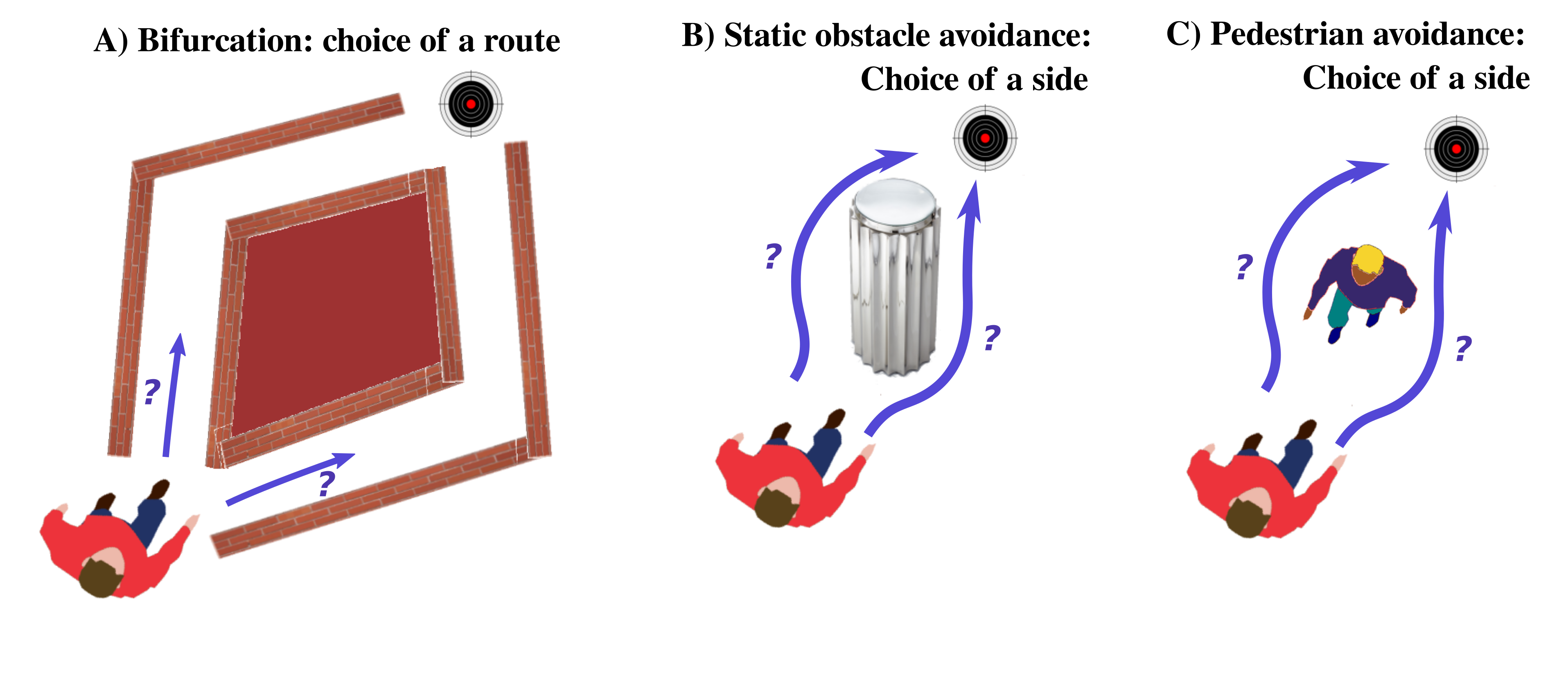
Figure 2.2: Route choice spans a continuum of decisions, from (a) actual routes to (b) obstacle avoidance, or even (c) pedestrian avoidance.

2.3 Modelling local navigation

Irrespective of the way in which pedestrian routes are implemented (via a road-map or a floor field as in Eq. 4), local pedestrian navigation will also require responding to the motion of neighbouring pedestrians. Naturally, the reason why these are more difficult to handle than static obstacles is that they are moving. Thus, in spacetime, they are not cylinders (invariant by translation along the time axis), but non-overlapping winding tubes (or tunnels) whose furtherances the agent has to predict in order to steer appropriately; see Fig. 2.3. This is dealt with by the integral extending into the future (in Eq. 2) in the game-theoretical approach, but at the expense of heavy computations (which prompted the development of mean-field versions of this approach [23, 28]).

At the other extreme, one may choose to determine each agent’s next velocity on the sole basis of their current neighours’ positions [29], as illustrated in Fig. 2.3(a). This leads to a reactive equation of motion akin to that of a driven passive particle [30], subject to distance-based interactions with its neighbours.

This alluringly simple approach, however, jettisons all the prediction capabilities of the agents (the other agents are then handled similarly to static obstacles, represented by time-invariant cylinders in space-time). To restore them partly while keeping in check the computational cost, methods based on the anticipated time to collision (TTC) have been put forward and validated empirically [31]. More precisely, the TTC is computed as the first time in the future at which a collision is expected if the neighbouring agents keep their current velocities. An expression for the TTC-based interaction energy was derived by Karamouzas and colleagues [31], in the form of a cut-off power law. In space-time, basing the potential on the TTC (which is a function of current positions and velocities) comes down to prolonging the other agents’ past trajectories as cylinders invariant along their current velocity vector $\boldsymbol{v}_{i}$ [Fig. 2.3(b)].

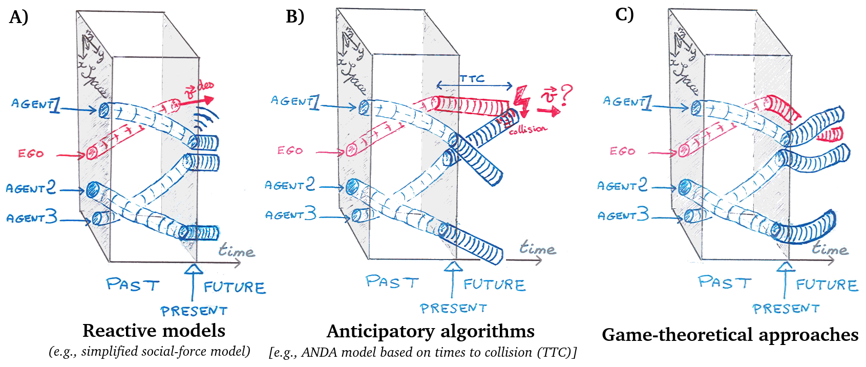
Figure 2.3: Schematic differences between different stems of agent-based models, highlighting their distinct extrapolations of the future. In this spacetime depiction, agents’ trajectories are represented as tubes.

2.4 Mechanics of locomotion and physical contacts

Pedestrian motion occupies a singular position among transport systems in that physical contacts can occur in close-to-normal flows at high densities. Thus, in addition to choices, mechanical effects need to be taken into account. In this respect, the motion of pedestrian $i$ (as a physical body of mass $m$ and position $\boldsymbol{r}_{i}$), averaged over a stepping cycle, is governed by Newton’s law of motion, viz.,

$$m\ddot{\boldsymbol{r}}_{i}=m\frac{\boldsymbol{u}_{i}^{\star}-\dot{\boldsymbol{r}_{i}}}{\tau^{\mathrm{mech}}}+\sum_{j\neq i}\boldsymbol{F}_{j\to i}^{\mathrm{c}}+\sum_{w\in\mathrm{walls}}\boldsymbol{F}_{w\to i}^{\mathrm{c}},$$ (5)

where $\boldsymbol{F}_{j\to i}^{\mathrm{c}}$ and $\boldsymbol{F}_{w\to i}^{\mathrm{c}}$ denote contact forces exerted by neighbouring pedestrians and walls, respectively. The first term of Eq. 5, which represents the controllable part of the acceleration [25] or the damped self-propelling force of an active particle, indicates that the desired velocity $\boldsymbol{u}_{i}^{\star}$ is not reached instantly, but only after characteristic time $\tau^{\mathrm{mech}}$ (a fraction of a second in free space) due to the cyclic human gait or the limited friction with the substrate. Importantly, $\tau^{\mathrm{mech}}$ only depends on locomotion and mechanical interactions, but on no account on the reaction time.

To elucidate this distinction between this mechanical relaxation time and the psychological reaction time, let us consider the example of a pedestrian walking on solid ground versus skating on an ice rink. While the reaction time of the pedestrian in both situations is the same, $\tau^{\mathrm{mech}}$ will be longer on the ice rink due to the more slippery surface; the skater will thus need more time to adjust their movements accordingly. To extrapolate to an even broader context, one may contrast the mechanical response time of a boat with that of a ground vehicle. Notably, $\tau^{\mathrm{mech}}$ is substantially higher for the former, reflecting the specifics of moving on water. These two examples from a broader context highlight the relevance of coupling the mechanical layer centred on Eq. 5 with a decision-making layer determining $\boldsymbol{u}_{i}^{\star}$, which is consistent with the early insight of [25], but quite generally overlooked in practice [29, 20, 31, 6].

Alternative approaches

Indeed, in conventional force-based models [15, 29, 31], pseudo-forces are additively inserted into Eq. 5 to account for the deviations from $\boldsymbol{u}_{i}^{\star}$ due to the local environment (other agents and walls). Conceptually, this is not satisfactory, because it puts these cognition-mediated effects on the same footing as mechanical forces, in particular subjecting them to the same relaxation time scale $\tau^{\mathrm{mech}}$. The conflation of mechanical and decisional processes is facilitated in practice by the fact that the cognitive reaction time $\tau_{\psi}$ involved in walking is of the same order of magnitude as $\tau^{\mathrm{mech}}$ and that both (cognitive and mechanical) processes take place within the confines of the same physical entity; the pedestrian. The confusion is much more conspicuous, but of the same nature, if one considers, instead of a pedestrian, a remote-controlled boat, for which $\tau_{\psi}\ll\tau^{\mathrm{mech}}$, and the control operator and the system are spatially separated.

3 Presentation of different types of models

After clarifying the conceptual foundations of major frameworks for agent-based pedestrian modelling and their differences, we aim to illustrate their implications in simulations and, for that purpose, this Section introduces archetypal examples for each of the three lines of models under consideration.

3.1 Game-theoretical model

In Sec. 2.2, we argued that the agent’s selection of a path, in interaction with their environment, can be handled as the optimisation of a generalised cost function (Eq. 2), subject to the concomitant path choices of other agents, hence a competition between the agents. This defines a ‘game’ in the mathematical sense [32]. While this assumption did not restrict the generality of the reasoning, here, to put forward a concrete, minimalistic model, we make further simplifications: we assume that all agents have the same type of cost function and that it takes the following simple form

$$C_{j}\Big{(}\boldsymbol{r}_{j}|\boldsymbol{r}_{-j}\Big{)}=\int_{t}^{t+T}\Big{(}\alpha\,v^{2}+\sum_{j\neq i}V(||\boldsymbol{r}_{ij}(t)||)\Big{)}dt^{\prime}+C_{j}^{T}(\boldsymbol{r}_{j}(T)),$$ (6)

where the term $\alpha\,v^{2}$ in the integrand penalises large speeds, $V$ is a simple repulsive distance-based potential, e.g., an exponential function $V(r)=V_{0}\exp{\Big{(}-r/r_{c}\Big{)}}$, and the terminal cost $C_{j}^{T}(\boldsymbol{r})=\pm Kx$, drives the agent to its goal (here going left or right). As the scale of the cost $C_{j}$ does not affect the position of its minimum, it can be rescaled so that $\alpha=1$. Besides, for an isolated agent, $V=0$, the cost $C_{j}$ in Eq. 6 is minimised for a speed $v=K/2$; therefore, the parameter $K$ can be set to $2v_{d}$, where $v_{d}$ is the agent’s preferential speed.

The game-theoretical problem is thus well defined. To find a Nash equilibrium, we solve Eq. 6 by splitting the cost $C_{j}$ into a short-term part over a time window $[t,t+dt]$ and the remaining cost $u(\boldsymbol{v},t+dt)=\inf_{\mathbf{v}}\int_{t+dt}^{t+T}\dots+C_{j}^{T}$ depending on the position $\boldsymbol{r}_{j}$ reached at time $t+dt$. This leads to Hamilton-Jacobi-Bellman equations for $u$, after neglecting higher-order terms:

$$0=\frac{\partial u}{\partial t}+\sum_{j\neq i}V(||\boldsymbol{r}_{ij}(t)||)-\frac{1}{4}(\nabla u)^{2},$$ (7)

with boundary condition $u(\boldsymbol{r},T)=C_{j}^{T}(\boldsymbol{r}_{j})$. Equation 7 is solved numerically over space and time. At each time step ($dt=0.05\,\mathrm{s}$), assuming that the other agent’s trajectory (hence $\boldsymbol{r}_{ij}$) is known, the optimal velocity is calculated as $\boldsymbol{v^{\star}}=\frac{-1}{2}\nabla_{\boldsymbol{r}}u$, after solving for $u(\boldsymbol{r},t)$ in Eq. 7 using an Euler finite-difference scheme in space and time, and starting from $t=T$; the amplification of numerical instabilities in the computation of derivatives is mitigated by smoothing the $u$-fields with a Gaussian kernel (with standard deviation 0.05 m). Supposing that no inertia is at play, the agent updates his or her position with $\boldsymbol{r}(t+dt)=\boldsymbol{r}(t)+\boldsymbol{v^{\star}}\,dt$.

We then proceed iteratively, starting from initial guesses of the two agents’ trajectories $\boldsymbol{r}_{i}(t)$ and $\boldsymbol{r}_{j}(t)$, and then updating $i$ and $j$ alternatively, until convergence. Note that initial guesses help to reach equilibrium trajectories faster but may constrain their shapes, as several Nash equilibria may exist. On the other hand, we have checked that the algorithm is robust to variations of $dt$ and that the aforementioned rescaling of the cost by $\alpha$ has no impact.

3.2 ANticipatory Dynamics Algorithm (ANDA)

The above optimisation of a full trajectory in relation with the rest of the crowd may become computationally costly for a crowd. To achieve a trade-off between this account of anticipation and numerical tractability, we turn to anticipatory models, and in particular the ANDA algorithm introduced in [24], which consists of a decision-making layer and a mechanical layer (given by Eq. 5). The desired velocity $\boldsymbol{u}_{i}^{\star}$ entering this equation is obtained from the decision-making layer as the velocity that minimises a cost function $E[\boldsymbol{u}]$ comprising several contributions (Eq. 8). We will briefly recall the main features of this function; for a detailed presentation of the model, the reader is referred to [24].

$$E[\boldsymbol{u}]={\color[rgb]{0.3333,0.6863,0.6784}E_{biomech}}+{\color[rgb]{0.9922,0.7490,0.4353}E_{FF}}+{\color[rgb]{0.3686,0.3098,0.6353}E_{inertia}}+{\color[rgb]{0.6196,0.0039,0.2588}E_{private-space}}+{\color[rgb]{0.9176,0.3647,0.2784}E_{anticipation}}$$ (8)

In free space, only the bio-mechanical contribution $E_{\mathrm{biomech}}$, measuring the (empirical) physiological cost of walking at a given speed $u=||\boldsymbol{u}||$ [33], the static floor field $E_{\mathrm{FF}}$ exposed in Section 3 (evaluated at the position that would be reached at the next time step with the test velocity $\boldsymbol{u}$), and the quadratic penalty $E_{\mathrm{inertia}}$ for changing velocities too abruptly are active. In uniform motion (i.e., no inertial effect), the chosen velocity is then directed along the gradient of $E_{\mathrm{FF}}$ and its magnitude $v^{\mathrm{pref}}$ minimises the sum of the first two contributions, as illustrated in Fig. 3.1. Accordingly, if one knows an agent’s free-walking speed $v^{\mathrm{pref}}$, the slope of the floor field can directly be obtained and the model contains no adjustable parameter at this point.

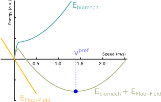
Figure 3.1: Variations of the bio-mechanical cost $E_{\mathrm{biomech}}$ (based on the data from [33]) and of the floor field $E_{\mathrm{FF}}$ with the test speed; by definition, the preferential speed $v^{\mathrm{pref}}$ minimises the sum of these two contributions.

On top of these three contributions, for pedestrians walking alone (no groups), interactions with the built environment and the crowd generate two new terms, reflecting two distinct types of repulsive interactions at play in pedestrian dynamics. The first one, $E_{\mathrm{private-space}}$, is based on the separation distance between an agent and their neighbours, with a short-ranged repulsive strength decaying with distance, which is familiar to physicists; it reflects the desire of people to preserve a private space around themselves, whose extent may vary between individuals and between cultures (as studied by the field of proxemics). Beyond these concerns for private space, pedestrians also pay particular attention to the risk of future collisions and adapt their trajectories to avoid them. Karamouzas et al. demonstrated, using empirical data sets, that these effects are much more readily described using a new variable, the anticipated time to collision (TTC), than distances [31].

In the ANDA model, we have kept this TTC-based energy, $E_{\mathrm{anticipation}}$, except that non-physical collisions between private spaces are also taken into account (which results in a smoother profile) and only the most imminent collision is considered.

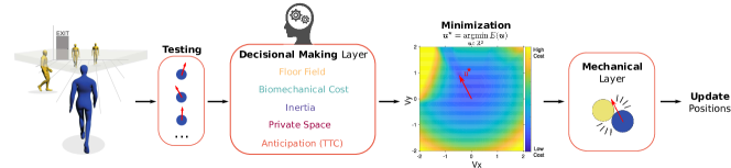
Figure 3.2: General functional diagram of the ANDA model.

This search for an optimal velocity $\boldsymbol{u}_{i}^{\star}$ minimising $E[\boldsymbol{u}_{i}]$ is done every $\tau_{\psi}$ seconds, which corresponds to the aforementioned cognitive reaction time. The actual velocity is then computed using the mechanical equation of motion, Eq. 5. In particular, it may happen that the selected desired velocity $\boldsymbol{u}_{i}^{\star}$ leads to a collision within $\tau_{\psi}$ and thus activates repulsive mechanical forces, an issue that we will not elaborate on here because the examples chosen below include no physical contacts.

Incidentally, the cost $E[\boldsymbol{u}_{i}]$ involves not only the test velocity $\boldsymbol{u}_{i}$ of agent $i$, but also the velocities $\boldsymbol{u}_{j}$ of the other agents, in particular $i$’s neighbours. Here, we posit that for these other agents the velocity to take into account is the current one, viz., $\boldsymbol{u}_{j}=\boldsymbol{v}_{j}(t)$, which comes down to assuming that agent $i$ furthers the other agents’ trajectories on the basis of the velocities that he or she currently observes. This assumption departs from what is typically done to determine equilibrium points in game theory, where each agent considers a situation in which the other agents’ choices are also optimal for them. Nevertheless, to lowest order in $\boldsymbol{\delta u}_{j}=\boldsymbol{u}_{j}(t+\delta t)-\boldsymbol{u}_{j}(t)$, the difference is transparent, insofar as a first-order expansion of $E[\boldsymbol{u}_{i}]$ only involves terms in $\boldsymbol{\delta u}_{i}$ and in $\boldsymbol{\delta u}_{j},\,j\neq i$ (no cross terms), and the latter do not affect the minimiser’s value $\boldsymbol{u}_{i}^{\star}$.

Overall, the model follows the functional diagram outlined in Fig. 3.2. There are only a few parameters (4 to 6, depending on how they are counted) that can be freely adjusted, including the spatial extent and the strength of the repulsion from the private space and the penalty for abrupt velocity changes.

3.3 Naïve social-force model

Finally, going all the way down the scale of complexity, we consider a reactive agent-based model. A classic paradigm of this category of models, the celebrated Social-Force-Model (SFM), hypothesizes that the local rules of navigation in a crowd system can be formalized by only using a mechanical layer identical to Eq. 5, which combines three different forces [29]. Formally, a pedestrian $i$ who wants to move in a particular direction $\hat{e}_{i}$ at a desired speed $\boldsymbol{v}_{d}$, is attracted to this destination by a driving force $\boldsymbol{f}^{D}_{i}$ which describes the adaptation of his/her current velocity $\dot{r}_{i}$ to his/her desired one as:

$$\boldsymbol{f}_{i}^{D}=\frac{\boldsymbol{v}_{d}-\dot{\boldsymbol{r}_{i}}}{\tau}$$ (9)

where $\tau$ is the time needed for the velocity adjustment ($\tau=0.4\,\mathrm{s}$ below). Importantly, in this expression both $\boldsymbol{v}_{d}$ and $\tau$ are parameters that remain constant over time, regardless of the conditions in which the pedestrian is found. Herein lies the main difference with the ANDA model, where, as explained above, the decisional layer provides the optimal value for the desired speed.

As pedestrian $i$ moves through the space, s/he is repelled by other pedestrians $j$ under the effect of a social force $\boldsymbol{f}^{S}_{ij}=-\boldsymbol{\nabla}V_{ij}(r_{ij})$ that mimics the interpersonal distances desired by people when walking. Thus, the ideal path that an isolated pedestrian would follow is permanently modulated by his/her tendency to move away from other individuals. For this purpose, here we use a long-range repulsive function decaying with distance, here $V_{ij}(r_{ij})=V_{0}\exp(-r_{ij}/r_{c})$, following [29] (note that a more sophisticated potential had been proposed in the first paper on SFM). Finally, physical contacts between agents might happen. To prevent pedestrians from overlapping either with each other or with walls, contact forces $\boldsymbol{f}^{C}_{ij}$ are introduced (but of little use for what follows).

Thus, at each instant $t$, the acceleration of a pedestrian is given by the sum of the internal and external forces to which (s)he is subjected, leading to an evolution of his/her speed as:

$$m_{i}\,\boldsymbol{\ddot{r}}_{i}=\boldsymbol{f}^{D}_{i}+\sum_{j\neq i}\boldsymbol{f}^{S}_{ij}(t)+\sum_{j\neq i}\boldsymbol{f}^{C}_{ij}(t)$$ (10)

This ordinary differential equation is solved numerically with time step $dt=0.05\,\mathrm{s}$.

4 Numerical comparison of the output in specific settings

After highlighting the conceptual discrepancies between the modelling branches, we will now make use of numerical simulations of the paradigmatic models exposed in the previous section to compare their output. While the scenarios under study could be multiplied ad infinitum, an emphasis will here be put on the simple, but ubiquitous task of binary collision avoidance, which allows for intuitive interpretation of the results.

4.1 Local navigation around complex static obstacles

Before turning to collision avoidance between distinct pedestrians, we study the avoidance of a static obstacle.

As mentioned above, this avoidance choice has an impact on the homotopy of the trajectory, which likens it to a tactical decision. However, in practice, the avoidance of small obstacles is often deferred to the operational module. In this case, the usual method consisting in first overlooking these small obstacles and prescribing the desired velocity towards an intermediate goal, and then taking the obstacles into account via repulsive pseudo-forces may fail drastically when these obstacles are of complex shape. This is illustrated with the simplified SFM in Fig. 4.1(a,c). Technically speaking, the obstacle was made of adjacent columns, each exerting the same repulsion as a static agent, $\|V_{ij}^{S}\|=V_{0}\exp(-r/r_{c})$), with $V_{0}=10$ and $r_{c}=1\,\mathrm{m}$. We observe that the agent is blocked ahead of the obstacle. Lowering the repulsion to $V_{0}=2$ is not conducive to a more realistic response for concave obstacles: the agent then succeeds in entering the concave shape but gets trapped in it [Fig. 4.1(c)]. Other agent-based models prescribing desired velocities independently of the obstacles would fail similarly [24].

On the other hand, within ANDA, the recourse a floor field $V(\boldsymbol{r})$ (or, more generally, to a value function $u(\boldsymbol{r},t)$ in game-theoretical approaches) sweeps away the distinction between local navigation and tactics. The extensive information about the geometry contained in the floor field naturally guides the agent around the obstacle, irrespective of its shape [Fig. 4.1(b,d).

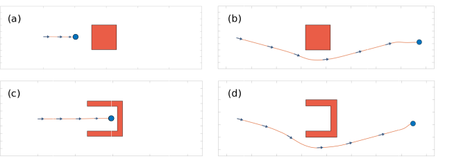
Figure 4.1: Avoidance of a static obstacle of convex square shape or non-convex shape. (a and c) SFM prediction for an agent walking at $v_{d}=1.5\,\mathrm{m/s}$; the obstacle is made of adjacent columns, each generating a potential (a) with high repulsion strength $V_{0}=10$ or (c) low strength ($V_{0}=2$) ; (b and d) Predictions of ANDA, for which the floor field integrates the effect of the obstacle.

4.2 Frontal collision avoidance

We now turn to collision avoidance between two pedestrians, with a particular interest in the qualitative features obtained when the desired speed is varied from slowly walking agents to people running towards one another. To simulate this scenario, we consider a scenario similar to the experiments of Moussaïd et al. [34], with two agents initially positioned at opposite ends of a corridor, about 10 meters away from one another and intent on reaching the other end of the corridor. Note that, in the three models under consideration, the increase in the desired speed reflects higher eagerness or hurry to reach the target, rather than a leisurely jogging session.

It has been shown that a SFM with forces spatially tailored in an ad hoc way can replicate the experimentally obtained mean trajectories for casually walking pedestrians [34]. These trajectories are also quantitatively reproduced by the ANDA model [24], as shown in Fig. 4.2(b).

With the simple SFM introduced above, without specific tailoring of the potenial $V$, the replication of the experiments is of course much poorer (Fig. 4.2, top row). For most parameters that have been tested, collisions are observed when the desired speed is increased. The only way to prevent a collision between the agents at all desired speeds is to impose a strong repulsion, $V_{0}=10$. Then, at moderate speeds, e.g., $v_{d}=1.5\mathrm{m/s}$, this leads to a sharp and strong detouring behaviour, represented in Fig. 4.2(c). More interesting are however the qualitative changes that occur when $v_{d}$ is further increased. As the interaction is only based on distance, the avoidance maneuver is then undertaken when collision is really imminent, i.e., much later than one would expect. Therefore, despite the repulsion strength, at $v_{d}=3\mathrm{m/s}$ the agents even fail to avoid one another, even though they started 10 meters away from each other.

The situation differs widely with ANDA: since short TTC (and not only short distances) are heavily penalised in the selection of an optimal velocity, the agents will start interacting farther and farther ahead as $v_{d}$ is increased, reflecting anticipation of the upcoming colllision. As a matter of fact, the spatial profiles of the trajectories in Fig. 4.2(b) do not change much when $v_{d}$ is varied: at higher $v_{d}$, at a given distance ahead of the collision point, the stronger TTC effect tends to be balanced by the higher eagerness to move forward. In any even, the agents manage to avoid collision in all these circumstances.

This also holds for the game-theoretical model, where the effect of varying $v_{d}$ is however felt slightly more strongly. This is due to the proportional increase of the cost driving the agent to its goal, which starts to dominate the repulsion with other agents. Technically speaking, here we considered a repulsive strength $V_{0}=1.1$, which provides acceptable results with respect to the empirical data. This parameter was chosen so as to minimise the distance between the experimental trajectory and the simulated one, measured in terms of the cumulative error between each simulated trajectory point the closest point of the real trajectory, and to reach an inter-agent distance when passing as close as possible to the experiments. Besides, note that we have added to the terminal cost $C^{T}$ a term $K_{y}\,\|y\|$ (with $K_{y}=1.5$), which pulls agents towards the central line, in order to limit their diffusion along the y-axis.

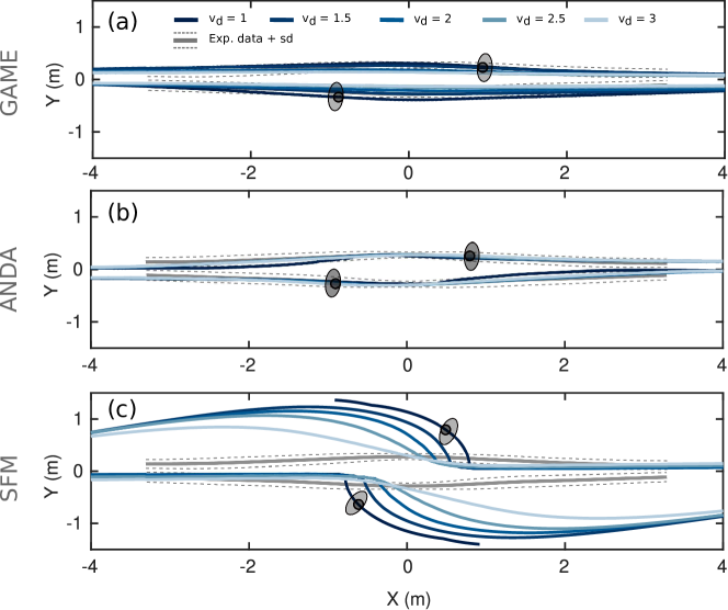
Figure 4.2: Collision avoidance by two counter-walking agents in a straight corridor, as a function of the preferential speed $v_{d}$. Numerical predictions based on (a) game theory, (b) ANDA, (c) SFM. The experimental data, drawn in gray, come from [34].

4.3 Effects of the characteristic times of the problem: distraction, mechanical friction, …

Let us now underscore the differences between the different timescales characterising pedestrian motion, which are best distinguished in ANDA.

The first timescale is the psychological reaction time $\tau_{\psi}$, depending on how often the agents refresh their perceptions of the environment (gazing activity) and need time to react in accordance; within ANDA, it is the time interval between updates of the desired velocity given by the decisional layer. Obviously, this time is expected to soar if the person is engaged in a discussion or playing with their smartphones (texting or web-browsing, in particular).

The consequences of this are illustrated in Fig. 4.3 for binary collision avoidance. While already visible at low walking speeds $v_{d}=1\,\mathrm{m/s}$, these consequences get even more striking at $v_{d}=2\,\mathrm{m/s}$. It is enlightening to confront these results with the experiments conducted by Murakami and colleagues [35]. In these experiments, a series of binary collision avoidance maneuvers was performed, in which one of the two pedestrians was sometimes asked to perform some complex activity on their smartphone while passing their counterpart. Interestingly, compared to the baseline with no smartphone distraction, the avoidance maneuver by distracted agent is undertaken later, but with a larger and more sudden reaction, which is qualitatively fully consistent with the numerical output of ANDA. Meanwhile, in the experiments, the non-distracted agent, who could not fully rely on mutual coordination for this avoidance, undertook a larger detour well in advance, so that the distance when passing the distracted agent is ultimately larger on average than with two non-distracted participants. With ANDA, it is also found that the distance when passing tends to increase with $\tau_{\psi}$: By responding with sufficient anticipation, gradual and limited adjustments of the velocity are sufficient, whereas abrupt detours may be needed if a collision is perceived only when it is imminent. Even though the foregoing comparison was limited to a very qualitative level, it can easily be understood that the ability to model digitally distracted pedestrians is vested with special interest in an overly connected society, where accidents due to smartphone-walking are on the surge.

The second timescale is the mechanical relaxation time $\tau^{\mathrm{mech}}$. Large $\tau^{\mathrm{mech}}$ denote a more inertial response, which would be typical of ice-skaters or swimmers, hence a difficulty to hold or recover one’s course if the presence of inertia is not internalised enough (bottom of Fig. 4.3). This echoes the advice given to sailors to steer the wheel smoothly and with anticipation.

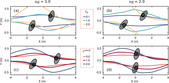
Figure 4.3: Effect of the psychological reaction time $\tau_{\psi}$ and the mechanical relaxation time $\tau^{\mathrm{mech}}$ on the collision avoidance between two agents in a straight corridor. First row (varying time-update) for vd = 1.0 m/s (a) and vd = 2.0 m/s (b). Second row (varying tau-mech) for vd = 1.0 m/s (c) and vd = 2.0 m/s (d).

5 Conclusion

In summary, we have examined the conceptual foundations of continuous pedestrian dynamics models. Starting from a broad context, we have argued that the articulation between the tactical and operational levels of description, which tends to coincide with the articulation between global path planning and local navigation, raises practical issues for modelling. While it is generally operated by defining intermediate way-points, the storage in memory of a ‘tactical’ floor field covering all space offers several advantages, particularly in the presence of obstacles or uncomfortable areas on the preferred paths. Our investigation has focused on three major branches of models, here dubbed reactive, anticipatory, and game-like; it has shed light on the simplifying assumptions under which a branch reduces to another one: differing in their predictions of the future, reactive agents, anticipative agents, and game players extrapolate future trajectories in spacetime in the form of time-invariant cylinders, cylinders, and flexible tubes, respectively.

For illustrative purposes, an archetypal example was chosen within each modelling branch: a simple SFM, the ANDA model, and a game in which agents interact via a distance-based repulsive potential. While the first one struggles to replicate head-on collision avoidance at various walking speeds, the latter two produce fairly similar collision-avoiding trajectories. Finally, the distinction between cognitive processes and mechanical contacts was underscored, at odds with the frequent amalgamation of the two notions in existing models. The effect of the timescales associated with these processes on collision avoidance was studied numerically; the trends predicted by ANDA when the reaction time is increased are qualitatively similar to those reported experimentally in [35], opening the door to numerical studies of the crowd dynamics of people distracted by their smartphones, a topic of particular relevance for pedestrian safety. More generally, the development of theoretically better grounded models is strongly advisable when it comes to exploring emerging situations for which one cannot fully rely on the (still scarce) data at hand.

Acknowledgments

We thank Matteo BUTANO for his particularly useful help with game theory. We acknowledge partial financial support by the Fédération d’Informatique de Lyon (CROSS project) and by the French National Research Agency (Agence Nationale de la Recherche, grant number ANR-20-CE92-0033) and the German Research Foundation (Deutsche Forschungsgemeinschaft DFG, grant number 446168800), in the frame of the French-German research project MADRAS.

References

- [1] L.A.J. Quetelet, Du système social et des lois qui le régissent (Guillaume, 1848)
- [2] L.A.J. Quetelet, Sur l’homme et le développement de ses facultés, ou Essai de physique sociale, vol. 2 (Bachelier, Imprimeur-libraire, 1869)
- [3] K. Pearson, Philosophical Transactions of the Royal Society of London. A 185, 71 (1894)
- [4] J. Von Neumann, O. Morgenstern, in Theory of games and economic behavior (Princeton university press, 1944)
- [5] M. Haghani, M. Coughlan, B. Crabb, A. Dierickx, C. Feliciani, R. van Gelder, P. Geoerg, N. Hocaoglu, S. Laws, R. Lovreglio, et al., Safety Science (in press) (2023)
- [6] B. Maury, S. Faure, Crowds in Equations: An Introduction to the Microscopic Modeling of Crowds (World Scientific, 2018)
- [7] A. Corbetta, F. Toschi, Annual Review of Condensed Matter Physics 14, 311 (2023)
- [8] J. Van Den Berg, S. Patil, J. Sewall, D. Manocha, M. Lin, in Proceedings of the 2008 symposium on Interactive 3D graphics and games (2008), pp. 139–147
- [9] J. Van den Berg, S.J. Guy, M. Lin, D. Manocha, in Robotics research (Springer, 2011), pp. 3–19
- [10] S. Curtis, Pedestrian velocity obstacles: Pedestrian simulation through reasoning in velocity space. Ph.D. thesis, The University of North Carolina at Chapel Hill (2013)
- [11] I. Karamouzas, N. Sohre, R. Narain, S.J. Guy, ACM Transactions on Graphics (TOG) 36(4), 1 (2017)
- [12] G. Antonini, M. Bierlaire, M. Weber, Transportation Research Part B: Methodological 40(8), 667 (2006)
- [13] T. Robin, G. Antonini, M. Bierlaire, J. Cruz, Transportation Research Part B: Methodological 43(1), 36 (2009)
- [14] M.J. Seitz, G. Köster, Physical Review E 86(4), 046108 (2012)
- [15] D. Helbing, P. Molnar, Physical review E 51(5), 4282 (1995)
- [16] M. Chraibi, A. Seyfried, A. Schadschneider, Physical Review E 82(4), 046111 (2010)
- [17] S. Seer, C. Rudloff, T. Matyus, N. Brändle, Transportation Research Procedia 2, 724 (2014)
- [18] X. Chen, M. Treiber, V. Kanagaraj, H. Li, Transport reviews 38(5), 625 (2018)
- [19] I.M. Sticco, G.A. Frank, F.E. Cornes, C.O. Dorso, Safety science 121, 42 (2020)
- [20] M. Moussaïd, D. Helbing, G. Theraulaz, Proceedings of the National Academy of Sciences 108(17), 6884 (2011)
- [21] I. Echeverría-Huarte, A. Nicolas, in Proceedings of the 2022 Traffic and Granular Flow Conference (Springer Nature, 2023 (in press))
- [22] S.P. Hoogendoorn, P.H. Bovy, Transportation Research Part B: Methodological 38(2), 169 (2004)
- [23] A. Lachapelle, M.T. Wolfram, Transportation research part B: methodological 45(10), 1572 (2011)
- [24] I. Echeverría-Huarte, A. Nicolas, arXiv preprint arXiv:2211.03419 (2022)
- [25] S. Hoogendoorn, P. HL Bovy, Optimal control applications and methods 24(3), 153 (2003)
- [26] N. Pelechano Gómez, K. O’Brien, B.G. Silverman, N. Badler, in First International Workshop on Crowd Simulation (2005)
- [27] T. Ikeda, Y. Chigodo, D. Rea, F. Zanlungo, M. Shiomi, T. Kanda, Robotics 10, 137 (2013)
- [28] T. Bonnemain, M. Butano, T. Bonnet, I. ía Huarte, A. Seguin, A. Nicolas, C. Appert-Rolland, D. Ullmo, Physical Review E 107(2), 024612 (2023)
- [29] D. Helbing, I. Farkas, T. Vicsek, Nature 407(6803), 487 (2000)
- [30] N. Bain, Hydrodynamics of polarized crowds: experiments and theory. Ph.D. thesis, École Normale Supérieure de Lyon (2018)
- [31] I. Karamouzas, B. Skinner, S.J. Guy, Physical review letters 113(23), 238701 (2014)
- [32] B. Maury, F. Al Reda, Comptes Rendus. Mathématique 359(9), 1071 (2021)
- [33] L.W. Ludlow, P.G. Weyand, Journal of Applied Physiology 120(5), 481 (2016)
- [34] M. Moussaïd, D. Helbing, S. Garnier, A. Johansson, M. Combe, G. Theraulaz, Proceedings of the Royal Society of London B: Biological Sciences pp. rspb–2009 (2009)
- [35] H. Murakami, T. Takenori, C. Feliciani, Y. Nishiyama, bioRxiv (2022)