Distributionally Robust Model Predictive Control:
Closed-loop Guarantees and Scalable Algorithms

Abstract.

We establish a collection of closed-loop guarantees and propose a scalable, Newton-type optimization algorithm for distributionally robust model predictive control (DRMPC) applied to linear systems, zero-mean disturbances, convex constraints, and quadratic costs. Via standard assumptions for the terminal cost and constraint, we establish distribtionally robust long-term and stage-wise performance guarantees for the closed-loop system. We further demonstrate that a common choice of the terminal cost, i.e., as the solution to the discrete-algebraic Riccati equation, renders the origin input-to-state stable for the closed-loop system. This choice of the terminal cost also ensures that the exact long-term performance of the closed-loop system is independent of the choice of ambiguity set the for DRMPC formulation. Thus, we establish conditions under which DRMPC does not provide a long-term performance benefit relative to stochastic MPC (SMPC). To solve the proposed DRMPC optimization problem, we propose a Newton-type algorithm that empirically achieves superlinear convergence by solving a quadratic program at each iteration and guarantees the feasibility of each iterate. We demonstrate the implications of the closed-loop guarantees and the scalability of the proposed algorithm via two examples.

Keywords. Model predictive control, distributionally robust optimization, closed-loop stability, second-order algorithms

1. Introduction

Model predictive control (MPC) defines an implicit control law via a finite horizon optimal control problem. This optimal control problem is defined by the stage cost $\ell(x,u)$, state/input constraints, and a (discrete-time) dynamical model:

$$x^{+}=f(x,u,w)$$

in which $x$ is the state, $u$ is the manipulated input, and $w$ is the disturbance. The primary difference between variants of this general MPC formulation (e.g., nominal, robust, and stochastic MPC) is their approach to modeling the disturbance $w$ in the optimization problem.

In nominal MPC, the optimization problem uses a nominal dynamical model, i.e., $w=0$. Nonetheless, feedback affords nominal MPC a nonzero margin of inherent robustness to disturbances [13, 37, 1]. This nonzero margin, however, may be insufficient in certain safety-critical applications with high uncertainty. Robust MPC (RMPC) and stochastic MPC (SMPC) offer a potential means to improve on the inherent robustness of nominal MPC by characterizing the disturbance and including this information in the optimal control problem.

RMPC describes the disturbance via a set $\mathbb{W}$ and requires that the state and input constraints in the optimization problem are satisfied for all possible realizations of $w\in\mathbb{W}$. The objective function of RMPC considers only the nominal system ($w=0$) and these methods are sometimes called tube-based MPC if the constraint tightening is computed offline [21, 12].

SMPC includes a stochastic description of the disturbance $w\sim\mathds{P}$ ($w$ is distributed according to the probability distribution $\mathds{P}$) and defines the objective function based on the expected value of the cost function subject to this distribution [5, 8, 23, 17]. This stochastic description of the disturbance also permits the use of so-called chance constraints. The performance of SMPC therefore depends on the disturbance distribution $\mathds{P}$. Analogous to nominal MPC, feedback affords SMPC a small margin of inherent distributional robustness, i.e., robustness to inaccuracies in the disturbance distribution [22]. If this distribution is identified from limited data, however, there may be significant distributional uncertainty. Therefore, a distributionally robust (DR) approach to the SMPC optimization problem may provide desirable benefits in applications with high uncertainty and limited data.

Advances in distributionally robust optimization (DRO) have inspired a range of distributionally robust MPC (DRMPC) formulations. In general, these problems take the following form:

$$\min_{\theta\in\Pi(x)}\max_{\mathds{P}\in\mathcal{P}}\mathbb{E}_{\mathds{P}}[J(x,\theta,\mathbf{w})]$$ (1)

in which $x$ is the current state of the system, $\theta$ defines the control inputs for the MPC horizon (potentially as parameters in a previously defined feedback law), $\mathbb{E}_{\mathds{P}}\left[\cdot\right]$ denotes the expected value with respect to the distribution $\mathds{P}$, and $\mathcal{P}$ is the ambiguity set for the distribution $\mathds{P}$ of the disturbances $\mathbf{w}$. The goal is to select $\theta$ to minimize the worst-case expected value of the cost function $J(\cdot)$ and satisfy the (chance-)constraints embedded in the set $\Pi(x)$. Note that SMPC and RMPC are special cases of DRMPC via specific choices of $\mathcal{P}$.

The key feature of all MPC formulations is that the finite horizon optimal control problem in 1 is solved with an updated state estimate at each time step, i.e., a rolling horizon approach. With this approach, DRMPC defines an implicit feedback control law $\kappa(x)$ and the closed-loop system

$$x^{+}=f(x,\kappa(x),w)$$ (2)

The performance of this controller is ultimately defined by this closed-loop system and the stage cost. In particular, we often define performance based on the expected average closed-loop stage cost at time $k\geq 1$, i.e.,

$$\mathcal{J}_{k}(\mathds{P}):=\mathbb{E}_{\mathds{P}}\left[\frac{1}{k}\sum_{i=0}^{k-1}\ell\Big{(}\phi(i),\kappa(\phi(i))\Big{)}\right]$$

in which $\phi(i)$ is the closed-loop state trajectory defined by 2 and $\mathds{P}$ is the distribution for the closed-loop disturbance.

In this work, we focus on DRMPC formulations for linear systems with additive disturbances and quadratic costs. We note that there are also DRMPC formulations that consider parameteric uncertainty [7] and piecewise affine cost functions are also considered in [24]. In both cases, the proposed DRMPC formulation solves for only a single input trajectory for all realizations of the disturbance.

To better address the realization of uncertainty in the open-loop trajectory, RMPC/SMPC formulations typically solve for a trajectory of parameterized control policies instead of a single input trajectory. A common choice of this parameterization is the state-feedback law $u=Kx+v$ in which $K$ is the fixed feedback gain and the parameter to be optimized is $v$. Using this parameterization, several DRMPC formulations were proposed to tighten probabilistic constraints for linear systems based on different ambiguity sets [19, 34, 9, 16]. In these formulations, however, the cost function is unaltered from the corresponding SMPC formulation due to the fixed feedback gain in the control law parameterization.

If the control law parameterization is chosen as a more flexible feedback affine policy (see 8), first proposed for MPC formulations in [12], distributional uncertainty in the cost function is nontrivial to the DRMPC problem. Van Parys et al. [36] propose a tractable method to solve linear quadratic control problems with unconstrained inputs and a distributionally robust chance constraint on the state. Coppens and Patrinos [6] consider a disturbance feedback affine parameterization with conic representable ambiguity sets and demonstrate a tractable reformulation of the DRMPC problem. Mark and Liu [20] consider a similar formulation with a simplified ambiguity set and also establish some performance guarantees for the closed-loop system. Taşkesen et al. [35] demonstrate that for unconstrained linear systems, additive disturbances, and quadratic costs, a linear feedback law is optimal and can be found via a semidefinite program (SDP). Pan and Faulwasser [28] use polynomial chaos expansion to approximate and solve the distributionally robust optimal control problem.

While these new formulations are interesting, there remain important questions about the efficacy of including yet another layer of uncertainty in the MPC problem. For example, what properties should DRMPC provide to the closed-loop system in 2? And what conditions are required to achieve these properties? Due to the rolling horizon nature of DRMPC, distributionally robust closed-loop properties are not necessarily obtained by simply solving a distributional robust optimization problem. Moreover, the conditions under which DRMPC provides significant performance benefits relative to SMPC are currently unknown. One of the main contributions of this paper is to provide greater insight into these questions. The focus, in particular, is on the performance benefits and guarantees that may be obtained by considering distributional uncertainty in the cost function 1. Chance constraints are therefore not considered in the proposed DRMPC formulation or closed-loop analysis.

DRMPC is also limited by practical concerns related to the computational cost of solving DRO problems. While these DRMPC problems can often be reformulated as convex optimization problems, in particular SDPs, these optimization problems are often significantly more difficult to solve relative to the quadratic programs (QPs) that are ubiquitous in nominal, robust, and stochastic MPC problems.

In this work, we consider a DRMPC formulation for linear dynamical models, additive disturbances, convex constraints, and quadratic costs. This DRMPC formulation uses a Gelbrich ambiguity set with fixed first moment (zero mean) as a conservative approximation for a Wasserstein ball of the same radius [10]. The key contributions of this work are (informally) summarized in the following two categories.

1. Closed-loop guarantees:

   1. Distributionally robust long-term performance. We establish sufficient conditions for DRMPC, in particular the terminal cost and constraint, such that the closed-loop system satisfies a distributionally robust long-term performance bound (Theorem 3.1), i.e., we define a function $C(\mathds{P})$ such that

      $$\limsup_{k\rightarrow\infty}\mathcal{J}_{k}(\mathds{P})\leq\max_{\tilde{\mathds{P}}\in\mathcal{P}}C(\tilde{\mathds{P}})$$ (3)

      for all $\mathds{P}\in\mathcal{P}$. This bound is distributionally robust because it holds for all distributions $\mathds{P}\in\mathcal{P}$.

   2. Distributionally robust stage-wise performance. If the stage cost is also positive definite, we establish that the closed-loop system satisfies a distributionally robust stage-wise performance bound (Theorem 3.2), i.e., there exists $\lambda\in(0,1)$ and $c,\gamma>0$ such that

      $$\mathbb{E}_{\mathds{P}}\left[\ell\Big{(}\phi(k),\kappa(\phi(k))\Big{)}\right]\leq\lambda^{k}c|\phi(0)|^{2}+\max_{\tilde{\mathds{P}}\in\mathcal{P}}\gamma C(\tilde{\mathds{P}})$$ (4)

      for all $\mathds{P}\in\mathcal{P}$. Moreover, this result directly implies that the closed-loop system is distributionally robust, mean-squared input-to-state stable (ISS) (Corollary 3.3), i.e., the left-hand side of 4 becomes $\mathbb{E}_{\mathds{P}}\left[|\phi(k)|^{2}\right]$.

   3. Pathwise input-to-state stability. A common approach in MPC design is to select the terminal cost based on the discrete-algebraic riccati equation (DARE) for the unconstrained linear system. Under these conditions, we establish that the closed-loop system is in fact (pathwise) ISS (Theorem 3.4), which is a stronger property than mean-squared ISS.

   4. Exact long-term performance. Given this stronger property of (pathwise) ISS, we can further establish an exact value for the long-term performance of DRMPC based on this terminal cost and the closed-loop disturbance distribution (Theorem 3.5), i.e.,

      $$\lim_{k\rightarrow\infty}\mathcal{J}_{k}(\mathds{P})=C(\mathds{P})$$ (5)

      for all distributions $\mathds{P}$ supported on $\mathbb{W}$. Of particular interest is the fact that this result is independent of the choice of ambiguity set $\mathcal{P}$. Thus, the long-term performance of DRMPC, SMPC, and RMPC are equivalent for this choice of terminal cost (Corollary 3.6).

2. Scalable algorithm: Newton-type saddle point algorithm. We present a novel optimization algorithm tailored to solve the DRMPC problem of interest (Algorithm 1). In contrast to Frank-Wolfe algorithms previously proposed to solve DRO problems (e.g., [27, 32]), the proposed algorithm solves a QP at each iteration instead of an LP. The Newton-type algorithm achieves superlinear (potentially quadratic) convergence in numerical experiments (Figure 1) and reduces computation time 50% compared to solving the DRMPC problem as an LMI optimization problem with state-of-the art solvers, i.e., MOSEK (Figure 2).

Organization

In Section 2, we introduce the DRMPC problem formulation and associated DRO problem. In Section 3, we present the main technical results on closed-loop guarantees. In Section 4, we provide the technical proofs and supporting lemmata for the main technical results introduced in Section 3. In Section 5, we discuss the DRO problem of interest and introduce the proposed Newton-type saddle point algorithm. In Section 6, we study two examples to demonstrate the closed-loop properties established in Section 3 and the scalability of the proposed algorithm.

Notation

Let $\mathbb{R}$ denote the reals and subscripts/superscripts denote the restrictions/dimensions for the reals, i.e., $\mathbb{R}^{n}_{\geq 0}$ is the set of nonegative reals with dimension $n$. The transpose of a square matrix $M\in\mathbb{R}^{n\times n}$ is denoted $M^{\prime}$. The trace of a matrix $M\in\mathbb{R}^{n\times n}$ is denoted $\textnormal{tr}(M)$. A positive (semi)definite matrix $M\in\mathbb{R}^{n\times n}$ is denoted by $M\succ 0$ ($M\succeq 0$). For $M\succeq 0$, let $|x|_{M}^{2}$ denote the quadratic form $x^{\prime}Mx$. If $\mathds{P}$ is a probability distribution, $\mathds{P}(A)$ denotes the probability of event $A$. Let $\mathbb{E}_{\mathds{P}}\left[\cdot\right]$ denote the expected value with respect to $\mathds{P}$. Let $\mathbb{E}_{\mathds{P}}\left[\cdot\mid x\right]$ denote the expected value with respect to $\mathds{P}$ and given the value of $x$. A function $\alpha:\mathbb{R}_{\geq 0}\rightarrow\mathbb{R}_{\geq 0}$ is said to be in class $\mathcal{K}$, denoted $\alpha(\cdot)\in\mathcal{K}$, if $\alpha(\cdot)$ is continuous, strictly increasing, and $\alpha(0)=0$.

2. Problem Formulation

We consider the linear system with additive disturbances

$$x^{+}=Ax+Bu+Gw$$ (6)

in which $x\in\mathbb{R}^{n}$, $u\in\mathbb{U}\subseteq\mathbb{R}^{m}$, and $w\in\mathbb{W}\subseteq\mathbb{R}^{q}$. We also consider the state/input constraints

$$(x,u)\in\mathbb{Z}\subseteq\mathbb{R}^{n}\times\mathbb{U}$$ (7)

and the terminal constraint $\mathbb{X}_{f}\subseteq\mathbb{R}^{n}$. We consider convex constraints as follows.

Assumption 2.1 (Convex state-action constraints).

The sets $\mathbb{Z}$ and $\mathbb{X}_{f}$ are closed, convex, and contain the origin in their interior. The set $\mathbb{U}$ is compact and contains the origin. The set $\mathbb{W}$ is compact and contains the origin in its interior.

To ensure constraint satisfaction, we use the following disturbance feedback parameterization [12].

$$u(i)=v(i)+\sum_{j=0}^{i-1}M(i,j)w(j)$$ (8)

in which $v(i)\in\mathbb{R}^{m}$ and $M(i,j)\in\mathbb{R}^{m\times q}$. With this parameterization and a finite horizon $N\geq 1$, the input sequence $\mathbf{u}:=(u(0),u(1),\dots,u(N-1))$ is defined as

$$\mathbf{u}=\mathbf{M}\mathbf{w}+\mathbf{v}$$ (9)

in which $\mathbf{w}:=(w(0),w(1),\dots,w(N-1))$ is the disturbance trajectory. Note that the structure of $\mathbf{M}$ must satisfy the following requirements to enforce causality.

$$(\mathbf{M},\mathbf{v})\in\Theta:=\left\{(\mathbf{M},\mathbf{v})\ \middle|\ \begin{matrix}\mathbf{M}\in\mathbb{R}^{Nm\times Nq},\ \mathbf{v}\in\mathbb{R}^{Nm}\\ \ M(i,j)=0\ \forall j\geq i\end{matrix}\right\}$$

The state trajectory $\mathbf{x}:=(x(0),x(1),\dots,x(N))$ is therefore

$$\mathbf{x}=\mathbf{A}x+\mathbf{B}\mathbf{v}+(\mathbf{B}\mathbf{M}+\mathbf{G})\mathbf{w}$$ (10)

and the constraints for this parameterization are given by

$$\Pi(x):=\bigcap_{\mathbf{w}\in\mathbb{W}^{N}}\left\{(\mathbf{M},\mathbf{v})\in\Theta\ \middle|\ \begin{matrix}\textnormal{s.t. }\lx@cref{creftype~refnum}{eq:bfu},\ \lx@cref{creftype~refnum}{eq:bfx}\\ (x(k),u(k))\in\mathbb{Z}\ \forall\ k\\ x(N)\in\mathbb{X}_{f}\end{matrix}\right\}$$

That is, if $(\mathbf{M},\mathbf{v})\in\Pi(x)$ then the constraints in 7 are satisfied for all realizations of the disturbance trajectory $\mathbf{w}\in\mathbb{W}^{N}$. We also define the feasible set

$$\mathcal{X}:=\{x\in\mathbb{R}^{n}\mid\Pi(x)\neq\emptyset\}$$

To streamline notation, we define

$$\theta:=(\mathbf{M},\mathbf{v})\in\Pi(x)$$

Lemma 2.1 (Policy constraints).

If Assumption 2.1 holds, then $\Pi(x)$ is compact and convex for all $x\in\mathcal{X}$ and $\mathcal{X}$ is closed and convex.

See Appendix A for the proof. Note that Lemma 2.1 uses a slightly different formulation and set of assumptions than in [12], and we are therefore able to establish that $\Pi(x)$ is also bounded. Moreover, if $\mathbb{Z}$ and $\mathbb{X}_{f}$ are polyhedral and $\mathbb{W}$ is a polytope, then $\Pi(x)$ is also a (bounded) polytope [12].

For the MPC problem, we consider quadratic stage and terminal costs defined as

$$\ell(x,u)=x^{\prime}Qx+u^{\prime}Ru\qquad V_{f}(x)=x^{\prime}Px$$

with the following standard assumption.

Assumption 2.2 (Positive semidefinite cost).

The matrices $Q$ and $P$ are positive semidefinite ($Q,P\succeq 0$) and $R$ is positive definite ($R\succ 0$).

For a given input and disturbance trajectory, we have the following deterministic cost function.

$$\Phi(x,\mathbf{u},\mathbf{w}):=\sum_{k=0}^{N-1}\ell(x(k),u(k))+V_{f}(x(N))$$

If we embed the disturbance feedback parameterization in this cost function, we have

$$J(x,\theta,\mathbf{w}):=\Phi(x,\mathbf{M}\mathbf{w}+\mathbf{v},\mathbf{w})=|H_{x}x+H_{u}\mathbf{v}+(H_{u}\mathbf{M}+H_{w})\mathbf{w}|^{2}$$

with constant matrices $H_{x}$, $H_{u}$, and $H_{w}$.

We make the following standing assumption for the remainder of this paper: The disturbances $w$ are zero mean, independent in time, and satisfy $w\in\mathbb{W}$ with probability one. Let $\mathcal{M}(\mathbb{W})$ denote all probability distributions of the random variable $w$ with zero mean such that $w\in\mathbb{W}$ with probability one, i.e.,

$$\mathcal{M}(\mathbb{W}):=\left\{\mathds{P}\ \middle|\ \mathbb{E}_{\mathds{P}}\left[w\right]=0,\ \mathds{P}\left(w\in\mathbb{W}\right)=1\right\}$$

For any distribution $\mathds{P}\in\mathcal{M}(\mathbb{W}^{N})$ of $\mathbf{w}$ with covariance $\boldsymbol{\Sigma}:=\mathbb{E}_{\mathds{P}}\left[\mathbf{w}\mathbf{w}^{\prime}\right]$, we have

$$L(x,\theta,\boldsymbol{\Sigma}):=\mathbb{E}_{\mathds{P}}\left[J(x,\theta,\mathbf{w})\right]=|H_{x}x+H_{u}\mathbf{v}|^{2}+\textnormal{tr}\Big{(}(H_{u}\mathbf{M}+H_{w})^{\prime}(H_{u}\mathbf{M}+H_{w})\boldsymbol{\Sigma}\Big{)}$$ (11)

Note that $L(x,\theta,\boldsymbol{\Sigma})$ is quadratic in $\theta$ and linear in $\boldsymbol{\Sigma}$. In SMPC, we minimize $L(x,\theta,\boldsymbol{\Sigma})$ for a specific covariance $\boldsymbol{\Sigma}$ and the current state $x$.

For DRMPC, we instead consider a worst-case version of the SMPC problem in which $\mathds{P}$ takes the worst value within some ambiguity set. To define this ambiguity set, we first consider the Gelbrich ball for the covariance of a single disturbance $w\in\mathbb{R}^{q}$ centered at the nominal covariance $\widehat{\Sigma}\in\mathbb{R}^{q\times q}$ with radius $\varepsilon\geq 0$ defined as

$$\mathbb{B}_{\varepsilon}(\widehat{\Sigma}):=\left\{\Sigma\succeq 0\ \middle|\ \textnormal{tr}\left(\widehat{\Sigma}+\Sigma-2\left(\widehat{\Sigma}^{1/2}\Sigma\widehat{\Sigma}^{1/2}\right)^{1/2}\right)\leq\varepsilon^{2}\right\}$$

To streamline notation, we define

$$\mathbb{B}_{d}:=\mathbb{B}_{\varepsilon}(\widehat{\Sigma}),\qquad\text{where}\qquad d:=\left(\varepsilon,\widehat{\Sigma}\right)$$

This Gelbrich ball produces the following Gelbrich ambiguity set for the distributions of $w$:

$$\mathcal{P}_{d}:=\left\{\mathds{P}\in\mathcal{M}(\mathbb{W})\ \middle|\ \mathbb{E}_{\mathds{P}}[ww^{\prime}]=\Sigma\in\mathbb{B}_{d}\right\}$$

We further assume that this Gelbrich ambiguity set is compatible with $\mathbb{W}$, i.e., all covariances $\Sigma\in\mathbb{B}_{d}$ can be achieved by at least one distribution $\mathds{P}\in\mathcal{M}(\mathbb{W})$. For example, in the extreme case that $\mathbb{W}=\{0\}$ then $\mathcal{M}(\mathbb{W})$ contains only one distribution with all the weight at zero and the only reasonable Gelbrich ball to consider is $\mathbb{B}_{d}=\{0\}$. Formally, we consider only ambiguity parameters $d\in\mathcal{D}$ with

$$\mathcal{D}:=\left\{(\varepsilon,\widehat{\Sigma})\ \middle|\begin{matrix}d=(\varepsilon,\widehat{\Sigma}),\ \varepsilon\geq 0,\ \widehat{\Sigma}\succeq 0,\\ \ \forall\ \Sigma\in\mathbb{B}_{d}\ \exists\ \mathds{P}\in\mathcal{M}(\mathbb{W})\ \textnormal{s.t. }\mathbb{E}_{\mathds{P}}[ww^{\prime}]=\Sigma\end{matrix}\right\}$$

Note that $\mathcal{D}$ depends on $\mathbb{W}$, but we suppress this dependence to streamline the notation. If $d\in\mathcal{D}$, then for any $\Sigma\in\mathbb{B}_{d}$ there exists $\mathds{P}\in\mathcal{P}_{d}$ such that $\mathbb{E}_{\mathds{P}}\left[ww^{\prime}\right]=\Sigma$.

For the disturbance trajectory $\mathbf{w}\in\mathbb{W}^{N}$, we define the following ambiguity set that enforces independence in time:

$$\mathcal{P}_{d}^{N}:=\prod_{k=0}^{N-1}\mathcal{P}_{d}=\left\{\mathds{P}\in\mathcal{M}(\mathbb{W}^{N})\ \middle|\ \begin{matrix}\mathbb{E}_{\mathds{P}}[w(k)w(k)^{\prime}]\in\mathbb{B}_{d}\\ w(k)\textrm{ are independent}\end{matrix}\right\}$$

We can equivalently represent $\mathcal{P}_{d}^{N}$ as

$$\mathcal{P}_{d}^{N}=\left\{\mathds{P}\in\mathcal{M}(\mathbb{W}^{N})\ \middle|\ \begin{matrix}\mathbb{E}_{\mathds{P}}\left[\mathbf{w}\mathbf{w}^{\prime}\right]=\boldsymbol{\Sigma}\in\mathbb{B}_{d}^{N}\\ w(k)\textrm{ are independent}\end{matrix}\right\}$$

in which the set $\mathbb{B}^{N}_{d}$ is defined as

$$\mathbb{B}^{N}_{d}:=\left\{\boldsymbol{\Sigma}=\begin{bmatrix}\Sigma_{0}&\dots&0\\ \vdots&\ddots&\vdots\\ 0&\dots&\Sigma_{N-1}\end{bmatrix}\ \middle|\ \Sigma_{k}\in\mathbb{B}_{d}\ \forall k\right\}$$

The worst-case expected cost is defined as

$$V_{d}(x,\theta):=\max_{\mathds{P}\in\mathcal{P}_{d}^{N}}\mathbb{E}_{\mathds{P}}\left[J(x,\theta,\mathbf{w})\right]=\max_{\boldsymbol{\Sigma}\in\mathbb{B}^{N}_{d}}L(x,\theta,\boldsymbol{\Sigma})$$ (12)

We note that equality between the two maximization problems in 12 holds because $d\in\mathcal{D}$. We now define the DRO problem for DRMPC as

$$V_{d}^{0}(x):=\min_{\theta\in\Pi(x)}\max_{\mathds{P}\in\mathcal{P}_{d}^{N}}\mathbb{E}_{\mathds{P}}\left[J(x,\theta,\mathbf{w})\right]=\min_{\theta\in\Pi(x)}V_{d}(x,\theta)$$ (13)

and we denote the solution(s) to the outer minimization problem as $\theta^{0}_{d}(x)$. Note that SMPC ($d=(0,\widehat{\Sigma})$) and RMPC ($d=(0,0)$) are special cases of the optimization problem in 13. Thus, all subsequent statements about DRMPC include SMPC and RMPC as special cases of $d\in\mathcal{D}$. Fundamental mathematical properties for this optimization problem (e.g., existence, continuity, and measurability) are provided in Appendix C.

3. Closed-loop guarantees: Main results

3.1. Preliminaries and closed-loop system

We now define the controller and closed-loop system derived from this DRMPC formulation. The control law is defined as the first input given by the optimal control law parameterization $\theta^{0}_{d}(x)$. Although $\theta^{0}_{d}(x)$ may be set-valued, i.e., there are multiple solutions, we assume that some selection rule is applied such that the control law $\kappa_{d}:\mathcal{X}\rightarrow\mathbb{U}$ is a single-valued function that satisfies

$$\kappa_{d}(x)\in\left\{v^{0}(0)\mid(\mathbf{M}^{0},\mathbf{v}^{0})\in\theta^{0}_{d}(x)\right\}$$

With this control law, the closed-loop system is

$$x^{+}=Ax+B\kappa_{d}(x)+Gw$$ (14)

Let $\phi_{d}(k;x,\mathbf{w}_{\infty})$ denote the closed-loop state of 14 at time $k\geq 0$, given the initial state $x\in\mathcal{X}$ and the disturbance trajectory $\mathbf{w}_{\infty}\in\mathbb{W}^{\infty}$, i.e., a disturbance trajectory in the $\ell^{\infty}$ space of sequences. Define the infinity norm of the sequence $\mathbf{w}_{\infty}$ as $||\mathbf{w}_{\infty}||:=\sup_{k\geq 0}|w(k)|$. Note that the deterministic value of $\phi_{d}(k;x,\mathbf{w}_{\infty})$ for a given realization of $\mathbf{w}_{\infty}\in\mathbb{W}^{\infty}$ is a function of $d\in\mathcal{D}$ via the DRMPC control law.

The goal of this section is to demonstrate the the closed-loop system in 14 obtains some desirable properties for the class of distributions considered in $\mathcal{P}_{d}$. We consider the set of all distributions for the infinite sequence of disturbances $\mathbf{w}_{\infty}$ such that the disturbances are independent in time and their marginal distributions are in $\mathcal{P}_{d}$, i.e., we consider the set

$$\mathcal{P}_{d}^{\infty}:=\prod_{k=0}^{\infty}\mathcal{P}_{d}=\left\{\mathds{P}\in\mathcal{M}(\mathbb{W}^{\infty})\ \middle|\ \begin{matrix}\mathbb{E}_{\mathds{P}}[w(k)w(k)^{\prime}]\in\mathbb{B}_{d}\\ w(k)\textrm{ are independent}\end{matrix}\right\}$$

An important property for the DRMPC algorithm is robust positive invariance, defined as follows.

Definition 3.1 (Robust positive invariance).

A set $X\subseteq\mathbb{R}^{n}$ is robustly positively invariant (RPI) for the system in 14 if $x^{+}\in X$ for all $x\in X$, $w\in\mathbb{W}$, and $d\in\mathcal{D}$.

Note that this definition is adapted for DRMPC to consider all possible $d\in\mathcal{D}$. If we choose $\mathcal{D}=\{(0,0)\}$ (RMPC) then this definition reduces to the standard definition of RPI found in, e.g., [30, Def 3.7]. Since the control law $\kappa_{d}:\mathcal{X}\rightarrow\mathbb{U}$ is defined on only the feasible set $\mathcal{X}$, the first step in the closed-loop analysis is to establish that this feasible set is RPI. We define the expected average performance of the closed-loop system for $k\geq 1$, given the initial state $x\in\mathcal{X}$, ambiguity parameters $d\in\mathcal{D}$, and the distribution $\mathds{P}\in\mathcal{P}_{d}^{\infty}$, as follows.

$$\mathcal{J}_{k}(x,d,\mathds{P}):=\mathbb{E}_{\mathds{P}}\left[\frac{1}{k}\sum_{i=0}^{k-1}\ell(\phi_{d}(i;x,\mathbf{w}_{\infty}),\kappa_{d}\Big{(}\phi_{d}(i;x,\mathbf{w}_{\infty}))\Big{)}\right]$$

3.2. Main results and key technical assumptions

To establish desirable properties for the closed-loop system, we consider the following assumption for the terminal cost $V_{f}(x)=x^{\prime}Px$ and constraint $\mathbb{X}_{f}$. This assumption is also used in SMPC and RMPC analysis.

Assumption 3.1 (Terminal cost and constraint).

The terminal cost matrix $P$ is chosen such that there exists $K_{f}\in\mathbb{R}^{m\times n}$ satisfying

$$P-Q-K_{f}^{\prime}RK_{f}\succeq(A+BK_{f})^{\prime}P(A+BK_{f})$$ (15)

Moreover, the terminal set $\mathbb{X}_{f}$ contains the origin in its interior and is chosen such that $(x,K_{f}x)\in\mathbb{Z}$ and $(A+BK_{f})x+Gw\in\mathbb{X}_{f}$ for all $x\in\mathbb{X}_{f}$ and $w\in\mathbb{W}$.

Verifying Assumption 3.1 is tantamount to finding a stabilizing linear control law $u=K_{f}x$, i.e., $A+BK_{f}$ is Schur stable, that satisfies the required constraints $(x,K_{f}x)\in\mathbb{Z}$ within some robustly positive invariant neighborhood of the origin $\mathbb{X}_{f}$. With this stabilizing linear control law, we can then construct an appropriate terminal cost matrix $P$ by, e.g., solving a discrete time Lyapunov equation. With this assumption, we can guarantee that the feasible set $\mathcal{X}$ is RPI and establish the following distributionally robust long-term performance guarantee. This performance guarantee is a distributionally robust version of the stochastic performance guarantee typically derived for SMPC (e.g., [17, 14, 5]).

Theorem 3.1 (DR long-term performance).

If Assumptions 2.1, 2.2 and 3.1 hold, then the set $\mathcal{X}$ is RPI for 14 and

$$\limsup_{k\rightarrow\infty}\mathcal{J}_{k}(x,d,\mathds{P})\leq\max_{\Sigma\in\mathbb{B}_{d}}\textnormal{tr}(G^{\prime}PG\Sigma)$$ (16)

for all $\mathds{P}\in\mathcal{P}^{\infty}_{d}$, $d\in\mathcal{D}$, and $x\in\mathcal{X}$.

Theorem 3.1, however, applies only to the average performance in the limit as $k\rightarrow\infty$. If we are also interested in the transient or stage-wise behavior of the closed-loop system at a given time $k\geq 0$, one can include the following assumption.

Assumption 3.2 (Positive definite stage cost).

The matrix $Q$ is positive definite, i.e., $Q\succ 0$. Moreover, the feasible set $\mathcal{X}$ is bounded or $\mathbb{X}_{f}=\mathbb{R}^{n}$.

By also including Assumption 3.2, we can establish the following distributionally robust stage-wise performance guarantee.

Theorem 3.2 (DR stage-wise performance).

If Assumptions 2.1, 2.2, 3.1 and 3.2 hold, then there exist $\lambda\in(0,1)$ and $c,\gamma>0$ such that

$$\mathbb{E}_{\mathds{P}}\left[\ell(x(k),u(k))\right]\leq\lambda^{k}c|x|^{2}+\gamma\left(\max_{\Sigma\in\mathbb{B}_{d}}\textnormal{tr}(G^{\prime}PG\Sigma)\right)$$ (17)

in which $x(k)=\phi_{d}(k;x,\mathbf{w}_{\infty})$, $u(k)=\kappa_{d}(x(k))$ for all $\mathds{P}\in\mathcal{P}^{\infty}_{d}$, $d\in\mathcal{D}$, $x\in\mathcal{X}$, and $k\geq 0$.

Theorem 3.2 ensures that the effect of the initial condition $x$ on the closed-loop stage cost vanishes exponentially fast as $k\rightarrow\infty$. There is also a persistent term on the right-hand side of 17 that accounts for the continuing effect of the disturbance. We note, however, that the persistent term on the right-hand side of 17 is a constant that depends on the design of the DRMPC algorithm and does not depend on the actual distribution $\mathds{P}$. Since $Q\succ 0$, we can also establish a the following corollary of Theorem 3.2.

Corollary 3.3 (DR, mean-squared ISS).

If Assumptions 2.1, 2.2, 3.1 and 3.2 hold, then there exist $\lambda\in(0,1)$ and $c,\gamma>0$ such that

$$\mathbb{E}_{\mathds{P}}\left[|\phi_{d}(k;x,\mathbf{w}_{\infty})|^{2}\right]\leq\lambda^{k}c|x|^{2}+\gamma\left(\max_{\Sigma\in\mathbb{B}_{d}}\textnormal{tr}(G^{\prime}PG\Sigma)\right)$$ (18)

for all $\mathds{P}\in\mathcal{P}^{\infty}_{d}$, $d\in\mathcal{D}$, $x\in\mathcal{X}$, and $k\geq 0$.

The ISS-style bound in 18 applies to the mean-squared norm of the closed-loop state, a commonly referenced quantity in stochastic stability analysis. Note that 18 also implies a similar bound for $\mathbb{E}_{\mathds{P}}\left[|\phi_{d}(k;x,\mathbf{w}_{\infty})|\right]$ via Jensen’s inequality. In MPC formulations, a common strategy is to choose the terminal cost matrix $P$ according to the discrete algebraic Riccati equation (DARE), i.e., the cost for the linear-quadratic regulator (LQR) of the unconstrained linear system. Specifically, we now consider the following stronger version of Assumption 3.1.

Assumption 3.3 (DARE terminal cost).

The matrix $P\succ 0$ satisfies

$$P=A^{\prime}PA-A^{\prime}PB(R+B^{\prime}PB)^{-1}B^{\prime}PA+Q$$ (19)

and $K_{f}:=-(R+B^{\prime}PB)B^{\prime}PA$. Moreover, $(x,K_{f}x)\in\mathbb{Z}$ and $(A+BK_{f})x+Gw\in\mathbb{X}_{f}$ for all $x\in\mathbb{X}_{f}$ and $w\in\mathbb{W}$. The terminal set $\mathbb{X}_{f}$ contains the origin in its interior.

With this stronger assumption, we can establish significantly stronger properties for the DRMPC controller, similar to results for SMPC reported in [11, Lemma 4.18]. In particular, we can establish that the closed-loop system is (pathwise) ISS.

Theorem 3.4 (Pathwise ISS).

Let Assumptions 2.1, 2.2, 3.2 and 3.3 hold. Then, for any $d\in\mathcal{D}$, the origin is (pathwise) ISS for 14, i.e., there exist $\lambda\in(0,1)$, $c>0$, and $\gamma(\cdot)\in\mathcal{K}$ such that

$$|\phi_{d}(k;x,\mathbf{w}_{\infty})|\leq\lambda^{k}c|x|+\gamma(||\mathbf{w}_{\infty}||)$$ (20)

for all $k\geq 0$, $\mathbf{w}_{\infty}\in\mathbb{W}^{\infty}$, and $x\in\mathcal{X}$.

The property of (pathwise) ISS in Theorem 3.4 is notably stronger than mean-squared ISS in Corollary 3.3. The key distinction is that the persistent term on the right-hand side of 20 is specific to a given realization of the disturbances trajectory $\mathbf{w}_{\infty}$, while the persistent term in Corollary 3.3 depends only on the DRMPC design. f $\mathbf{w}_{\infty}=\mathbf{0}$ then 20 implies that the origin is exponentially stable. By contrast, the weaker restriction on the terminal cost in Assumption 3.1 does not ensure that the closed-loop system is ISS. We demonstrate this fact in Section 6 via a counterexample.

We now consider a class of disturbances that are both independent and identically distributed (i.i.d.) in time. We also require that arbitrarily small values of these disturbances occur with nonzero probability. Specifically, we define the following set of distributions.

$$\mathcal{Q}:=\prod_{k=0}^{\infty}\left\{\mathds{P}\in\mathcal{M}(\mathbb{W})\ \middle|\ \forall\ \varepsilon>0,\ \mathds{P}(|w|\leq\varepsilon)>0\right\}$$

Note that $\mathcal{Q}$ includes most distributions of interest such as uniform, truncated Gaussian, and even finite distributions with $\mathds{P}(w=0)>0$. For this class of disturbances, we have the following exact long-term performance guarantee.

Theorem 3.5 (Exact long-term performance).

Let Assumptions 2.1, 2.2, 3.2 and 3.3 hold. Then,

$$\lim_{k\rightarrow\infty}\mathcal{J}_{k}(x,d,\mathds{P})=\textnormal{tr}(G^{\prime}PG\Sigma)$$ (21)

in which $\Sigma=\mathbb{E}_{\mathds{P}}\left[w(i)w(i)^{\prime}\right]$ for all $d\in\mathcal{D}$, $x\in\mathcal{X}$, and $\mathds{P}\in\mathcal{Q}$.

Note that 21 provides an exact value for the long-term performance based on the distribution of the disturbance in the closed-loop system. By contrast, 16 provides a conservative and constant bound based on the design parameter $d\in\mathcal{D}$. Furthermore, the values of $d\in\mathcal{D}$ do not affect the long-term performance in 21. By recalling that SMPC and RMPC are special cases of DRMPC, we have the following corollary of Theorem 3.5.

Corollary 3.6 (DRMPC versus SMPC).

If Assumptions 2.1, 2.2, 3.2 and 3.3 hold, then the long-term performance of DRMPC, SMPC ($\varepsilon=0$), and RMPC ($\varepsilon=0$, $\widehat{\Sigma}=0$) are equivalent, i.e.,

$$\lim_{k\rightarrow\infty}\mathcal{J}_{k}\Big{(}x,(\varepsilon,\widehat{\Sigma}),\mathds{P}\Big{)}=\lim_{k\rightarrow\infty}\mathcal{J}_{k}\Big{(}x,(0,\widehat{\Sigma}),\mathds{P}\Big{)}=\lim_{k\rightarrow\infty}\mathcal{J}_{k}\Big{(}x,(0,0),\mathds{P}\Big{)}$$

for all $x\in\mathcal{X}$, $\mathds{P}\in\mathcal{Q}$, and $(\varepsilon,\widehat{\Sigma})\in\mathcal{D}$.

Although selecting $P$ to satisfy 19 is a standard design method in MPC, there are also systems in which one cannot satisfy the requirements of Assumption 3.3 for a given $Q,R\succ 0$. In particular, if the origin is sufficiently close to (or on) the boundary of $\mathbb{Z}$, then satisfying all of the requirements in Assumption 3.3 is typically not possible. In chemical process control, for example, processes often operate near input constraints (e.g., maximum flow rates) to ensure high throughput for the process. Thus, the terminal cost and constraint are chosen to satisfy only the weaker condition in Assumption 3.1. In this case, there is a possibility that DRMPC produces superior long-term performance relative to SMPC and RMPC. We therefore focus on examples in Section 6 that satisfy Assumption 3.1, but cannot satisfy Assumption 3.3.

Remark 3.1 (Detectable stage cost).

We can also weaken Assumption 3.2 to $Q\succeq 0$ and $(A,Q^{1/2})$ detectable. By defining an input-output-to-state stability (IOSS) Lyapunov function, e.g., [30, Thm. 2.24 ], we can apply the same approach use for nominal MPC to establish Theorem 3.2 and Corollary 3.3 for DRMPC under this weaker restriction for $Q$.

4. Closed-loop guarantees: Technical proofs

This section includes several technical lemmata that serve as a preliminary to prove the main results of this study.

4.1. Distributionally robust long-term performance

To establish Theorem 3.1, we begin by establishing that feasible set $\mathcal{X}$ is RPI and providing a distributionally robust expected cost decrease condition.

Lemma 4.1 (DR cost decrease).

If Assumptions 2.1, 2.2 and 3.1 hold, then the feasible set $\mathcal{X}$ is RPI for 14 and

$$\mathbb{E}_{\mathds{P}}\left[V^{0}_{d}(x^{+})\right]\leq V^{0}_{d}(x)-\ell(x,\kappa_{d}(x))+\max_{\Sigma\in\mathbb{B}_{d}}\textnormal{tr}(G^{\prime}PG\Sigma)$$ (22)

for all $\mathds{P}\in\mathcal{P}_{d}$, $d\in\mathcal{D}$, and $x\in\mathcal{X}$.

Proof.

Choose $x(0)\in\mathcal{X}$ and $d\in\mathcal{D}$. Define $(\mathbf{M}^{0},\mathbf{v}^{0})=\theta^{0}\in\theta^{0}_{d}(x(0))$. Consider the subsequent state $x(1)=Ax(0)+Bv^{0}(0)+Gw(0)$ for some $w(0)\in\mathbb{W}$. For the state $x(1)$, we choose a candidate solution

$$\tilde{\theta}^{+}(w(0))=\Big{(}\tilde{\mathbf{M}}^{+},\tilde{\mathbf{v}}^{+}(w(0))\Big{)}$$ (23)

such that the open-loop input trajectory remains the same as the previous optimal solution, i.e.,

$$u(k)=v^{0}(k)+\sum_{j=0}^{k-1}M^{0}(k,j)w(j)=\tilde{v}^{+}(k)+\sum_{j=1}^{k-1}\tilde{M}^{+}(k,j)w(j)$$ (24)

for all $k\in\{1,\dots,N-1\}$ and $\mathbf{w}\in\mathbb{W}^{N}$. With this choice of parameters, the open-loop state trajectories $x(k)$ are also the same for all $k\in\{1,\dots,N-1\}$ and $\mathbf{w}\in\mathbb{W}^{N}$. The candidate solution is therefore

$$\tilde{\mathbf{M}}^{+}=\begin{bmatrix}0&\cdots&\cdots&0&0\\ M^{0}(2,1)&0&\cdots&0&0\\ \vdots&\ddots&\ddots&\vdots&\vdots\\ M^{0}(N-1,1)&\cdots&M^{0}(N-1,N-2)&0&0\\ \tilde{M}^{+}(N,1)&\cdots&\tilde{M}^{+}(N,N-2)&\tilde{M}^{+}(N,N-1)&0\end{bmatrix}$$

$$\tilde{\mathbf{v}}^{+}(w(0))=\begin{bmatrix}v^{0}(1)+M^{0}(1,0)w(0)\\ v^{0}(2)+M^{0}(2,0)w(0)\\ \vdots\\ v^{0}(N-1)+M^{0}(N-1,0)w(0)\\ \tilde{v}^{+}(N)\end{bmatrix}$$

in which that last rows of $\tilde{\mathbf{M}}^{+}$ and $\tilde{\mathbf{v}}^{+}(w(0))$ are not yet defined. We define these last rows by the terminal control law $u(N)=K_{f}x(N)$. Specifically, we have

$$K_{f}x(N)=\tilde{v}^{+}(N)+\sum_{i=1}^{N-1}\tilde{M}^{+}(N,i)w(i)$$ (25)

By definition of $x(N)$, we have

$$x(N)=A^{N-1}x(1)+\sum_{i=1}^{N-1}A^{N-1-i}\Big{(}Bu(i)+Gw(i)\Big{)}$$

We then substitute the values of $u(i)$ for the candidate solution in 24 to give

$$x(N)=A^{N-1}x(1) +\sum_{i=1}^{N-1}A^{N-1-i}B\Big{(}v^{0}(i)+M^{0}(i,0)w(0)\Big{)}$$

$$+\sum_{i=1}^{N-1}A^{N-1-i}\left(\sum_{j=1}^{i-1}BM^{0}(i,j)w(j)+Gw(i)\right)$$

With some manipulation, we can therefore define

$$\tilde{v}^{+}(N) =K_{f}A^{N-1}x(1)+\sum_{i=1}^{N-1}K_{f}A^{N-1-i}B\Big{(}v(i)+M^{0}(i,0)w(0)\Big{)}$$

$$\tilde{M}^{+}(N,i) =K_{f}\left(\sum_{j=i+1}^{N-1}A^{N-1-j}BM^{0}(j,i)+A^{N-1-i}G\right)$$

to satisfy 25. Note that $\tilde{\mathbf{M}}^{+}$ is independent of $w(0)$ and $\tilde{\mathbf{v}}^{+}(w(0))$ is an affine function of $w(0)$. We first establish that this candidate solution is feasible for any $w(0)\in\mathbb{W}$ and that $\mathcal{X}$ is RPI. Since $(\mathbf{M}^{0},\mathbf{v}^{0})\in\Pi(x(0))$, then $(x(k),u(k))\in\mathbb{Z}$ for all $k\in\{1,\dots,N-1\}$ and $x(N)\in\mathbb{X}_{f}$ for all $\mathbf{w}\in\mathbb{W}^{N}$. From Assumption 3.1, we also have that $(x(N),K_{f}x(N))\in\mathbb{Z}$ for all $\mathbf{w}\in\mathbb{W}^{N}$. Therefore, $(x(N),u(N))\in\mathbb{Z}$ and $x(N+1)=(A+BK_{f})x(N)+Gw(N)\in\mathbb{X}_{f}$ for all $w(N)\in\mathbb{W}$ by Assumption 3.1. Thus, $(\tilde{\mathbf{M}}^{+},\tilde{\mathbf{v}}^{+})\in\Pi(x(1))$. Since $\Pi(x(1))\neq\emptyset$, we also know that $x(1)\in\mathcal{X}$ for any $w(0)\in\mathbb{W}$. Since the choice of $x(0)\in\mathcal{X}$ and $d\in\mathcal{D}$ was arbitrary, we have that $\mathcal{X}$ is RPI. Choose $\mathbf{w}=(w(0),\dots,w(N-1))\in\mathbb{W}^{N}$ and define $\mathbf{w}^{+}=(w(1),\dots,w(N))$ with some additional $w(N)\in\mathbb{W}$. We have that

$$J(x(1),\tilde{\theta}^{+}(w(0)),\mathbf{w}^{+})-J(x(0),\theta^{0},\mathbf{w})=-\ell(x(0),v^{0}(0))\\ +V_{f}(x(N+1))-V_{f}(x(N))+\ell(x(N),K_{f}x(N))$$ (26)

We define

$$\boldsymbol{\Sigma}^{+} =\arg\max_{\boldsymbol{\Sigma}\in\mathbb{B}_{d}^{N}}L(x(1),\tilde{\theta}^{+}(w(0)),\boldsymbol{\Sigma})=\arg\max_{\boldsymbol{\Sigma}\in\mathbb{B}_{d}^{N}}\textnormal{tr}\left((H_{u}\tilde{\mathbf{M}}^{+}+H_{w})^{\prime}(H_{u}\tilde{\mathbf{M}}^{+}+H_{w})\boldsymbol{\Sigma}\right)$$

and note that $\boldsymbol{\Sigma}^{+}$ is independent of $w(0)$ because $\tilde{\mathbf{M}}^{+}$ is independent of $w(0)$. We also define the distribution $\mathds{Q}\in\mathcal{M}(\mathbb{W}^{N})$ for $\mathbf{w}^{+}$ such that $\mathbb{E}_{\mathds{Q}}[(\mathbf{w}^{+})(\mathbf{w}^{+})^{\prime}]=\boldsymbol{\Sigma}^{+}$. Note that such a $\mathds{Q}$ exists because $d\in\mathcal{D}$. For this distribution, we take the expected value of each side of 26 to give

$$\mathbb{E}_{\mathds{Q}}\left[J(x(1),\tilde{\theta}^{+}(w(0)),\mathbf{w}^{+})-J(x(0),\theta^{0},\mathbf{w})\mid w(0)\right]=\\ \mathbb{E}_{\mathds{Q}}\left[V_{f}(x(N+1))-V_{f}(x(N))+\ell(x(N),K_{f}x(N))\mid w(0)\right]-\ell(x(0),v^{0}(0))$$

From Assumption 3.1 and the fact that $x(N)\in\mathbb{X}_{f}$ for all $\mathbf{w}\in\mathbb{W}^{N}$, we have that

$$\mathbb{E}_{\mathds{Q}}\left[V_{f}(x(N+1))-V_{f}(x(N))+\ell(x(N),K_{f}x(N))\mid w(0)\right]\leq\textnormal{tr}(G^{\prime}PG\Sigma_{N})\leq\delta_{d}$$

in which $\Sigma_{N}=\mathbb{E}_{\mathds{Q}}[w(N)w(N)^{\prime}]\in\mathbb{B}_{d}$ and $\delta_{d}:=\max_{\Sigma\in\mathbb{B}_{d}}\textnormal{tr}(G^{\prime}PG\Sigma)$. From the definition of $\boldsymbol{\Sigma}^{+}$ and optimality, we have

$$V_{d}\Big{(}x(1),\tilde{\theta}^{+}(w(0))\Big{)}=\mathbb{E}_{\mathds{Q}}\left[J(x(1),\tilde{\theta}^{+}(w(0)),\mathbf{w}^{+})\mid w(0)\right]$$

and therefore

$$V_{d}\Big{(}x(1),\tilde{\theta}^{+}(w(0))\Big{)}\leq\mathbb{E}_{\mathds{Q}}\left[J(x(0),\theta^{0},\mathbf{w})\mid w(0)\right]-\ell(x(0),v^{0}(0))+\delta_{d}$$ (27)

Choose any $\mathds{P}\in\mathcal{P}_{d}$ for the distribution of $w(0)$. From the definition of $\mathds{P}$ and $\mathds{Q}$, we have

$$\mathbb{E}_{\mathds{P}}\left[\mathbb{E}_{\mathds{Q}}\left[J(x(0),\theta^{0},\mathbf{w})\mid w(0)\right]\right]\leq V_{d}(x(0),\theta^{0})=V^{0}_{d}(x(0))$$

because $\theta\in\theta^{0}_{d}(x(0))$. We take the expected value of 27 with respect to $\mathds{P}$ and use this inequality to give

$$\mathbb{E}_{\mathds{P}}\left[V_{d}\Big{(}x(1),\tilde{\theta}^{+}(w(0))\Big{)}\right]\leq V^{0}_{d}(x(0))-\ell(x(0),v^{0}(0))+\delta_{d}$$ (28)

By optimality, we have

$$V_{d}^{0}(x(1))\leq V_{d}\Big{(}x(1),\tilde{\theta}^{+}(w(0))\Big{)}$$

We combine this inequality with 28 and substitute in $x=x(0)$, $x^{+}=x(1)$, $\kappa_{d}(x)=v^{0}(0)$ to give 22. Note that the choices of $\mathds{P}\in\mathcal{P}_{d}$, $d\in\mathcal{D}$, and $x(0)\in\mathcal{X}$ were arbitrary and therefore 22 holds for all values in these sets. ∎

The key difference between Lemma 4.1 and the typical expected cost decrease condition for SMPC is that this inequality holds for all distributions $\mathds{P}\in\mathcal{P}_{d}$, i.e., the inequality is distributionally robust. We can then apply Lemma 4.1 to prove Theorem 3.1.

Proof of Theorem 3.1.

Choose $x\in\mathcal{X}$, $d\in\mathcal{D}$, and $\mathds{P}\in\mathcal{P}_{d}^{\infty}$. Define $x(i)=\phi_{d}(i;x,\mathbf{w}_{\infty})$ and $u(i)=\kappa_{d}(x(i))$. From Lemma 4.1, we have that $\mathcal{X}$ is RPI and

$$\mathbb{E}_{\mathds{Q}}\left[V^{0}_{d}(x(i+1))\mid x(i)\right]\leq V^{0}_{d}(x(i))-\ell(x(i),u(i))+\max_{\Sigma\in\mathbb{B}_{d}}\textnormal{tr}(G^{\prime}PG\Sigma)$$ (29)

for all $\mathds{Q}\in\mathcal{P}_{d}$. Let $\delta_{d}:=\max_{\Sigma\in\mathbb{B}_{d}}\textnormal{tr}(G^{\prime}PG\Sigma)$ to streamline notation. From the law of total expectation and 29, we have

$$\mathbb{E}_{\mathds{P}}\left[\ell(x(i),u(i))\right]\leq\mathbb{E}_{\mathds{P}}\left[V^{0}_{d}(x(i))\right]-\mathbb{E}_{\mathds{P}}\left[V^{0}_{d}(x(i+1))\right]+\delta_{d}$$

We sum both sides of this inequality from $i=0$ to $i=k-1$ and divide by $k\geq 1$ to give

$$\mathcal{J}_{k}(x,d,\mathds{P})\leq\frac{\mathbb{E}_{\mathds{P}}\left[V^{0}_{d}(x(0))\right]-\mathbb{E}_{\mathds{P}}\left[V^{0}_{d}(x(k))\right]}{k}+\delta_{d}$$

Note that $V^{0}_{d}(x(k))\geq 0$. We take the $\limsup$ as $k\rightarrow\infty$ of both sides of the inequality and substitute in the definition of $\delta_{d}$ to give 16. ∎

4.2. Distributionally robust stage-wise performance

To establish Theorem 3.2, we first establish the following upper bound for the optimal cost function.

Lemma 4.2 (Upper bound).

If Assumptions 2.1, 2.2, 3.1 and 3.2 hold, then

$$V^{0}_{d}(x)\leq c_{2}|x|^{2}+N\left(\max_{\Sigma\in\mathbb{B}_{d}}\textnormal{tr}(G^{\prime}PG\Sigma)\right)$$ (30)

for all $d\in\mathcal{D}$ and $x\in\mathcal{X}$.

Proof.

For any $x\in\mathbb{X}_{f}$, we define the control law as $u=K_{f}x$ from Assumption 3.1. Therefore,

$$\mathbf{u}=\mathbf{K}_{f}\mathbf{x},\quad\mathbf{x}=(I-\mathbf{B}\mathbf{K}_{f})^{-1}(\mathbf{A}x+\mathbf{G}\mathbf{w})$$

in which $\mathbf{K}_{f}:=\begin{bmatrix}I_{N}\otimes K_{f}&0\end{bmatrix}$. Note that the inverse $(I-\mathbf{B}\mathbf{K}_{f})^{-1}$ exists because $\mathbf{B}\mathbf{K}_{f}$ is nilpotent (lower triangular with zeros along the diagonal). We represent this control law as $\theta_{f}(x)=(\mathbf{M}_{f},\mathbf{v}_{f}(x))$ so that

$$\mathbf{v}_{f}(x):=\mathbf{K}_{f}(I-\mathbf{B}\mathbf{K}_{f})^{-1}\mathbf{A}x\qquad\mathbf{M}_{f}:=\mathbf{K}_{f}(I-\mathbf{B}\mathbf{K}_{f})^{-1}\mathbf{G}$$ (31)

We have from Assumption 3.1 that this control law ensures that $(x(k),u(k))\in\mathbb{Z}$ and $x(k+1)\in\mathbb{X}_{f}$ for all $k\in\{0,\dots,N-1\}$. Therefore $\theta_{f}(x)\in\Pi(x)$ for all $x\in\mathbb{X}_{f}$ and $d\in\mathcal{D}$. Choose any $x\in\mathbb{X}_{f}$ and $d\in\mathcal{D}$. Choose any $\boldsymbol{\Sigma}\in\mathbb{B}^{N}_{d}$ and corresponding $\mathds{P}\in\mathcal{P}_{d}^{N}$ such that $\mathbb{E}_{\mathds{P}}\left[\mathbf{w}\mathbf{w}^{\prime}\right]=\boldsymbol{\Sigma}$. From Assumption 3.1, we have that

$$\mathbb{E}_{\mathds{P}}\left[V_{f}(x(k+1))-V_{f}(x(k))+\ell(x(k),K_{f}x(k))\right]\leq\textnormal{tr}(G^{\prime}PG\Sigma_{k})\leq\delta_{d}$$

in which $x(k+1)=(A+BK_{f})x(k)+Gw(k)$ for all $k\in\{0,1,\dots,N-1\}$, $x(0)=x$, and $\delta_{d}:=\max_{\Sigma\in\mathbb{B}_{d}}\textnormal{tr}(G^{\prime}PG\Sigma)$. We sum both sides of this inequality from $k=0$ to $k=N-1$ and rearrange to give

$$L(x,\theta_{f}(x),\boldsymbol{\Sigma})\leq V_{f}(x(0))+N\delta_{d}$$

for all $\boldsymbol{\Sigma}\in\mathbb{B}^{N}_{d}$. Therefore,

$$V^{0}_{d}(x)\leq V_{d}(x,\theta_{f}(x))\leq V_{f}(x)+N\delta_{d}\leq\mathrm{bar}{\lambda}_{P}|x|^{2}+N\delta_{d}$$

in which $\mathrm{bar}{\lambda}_{P}$ is the maximum eigenvalue of $P$ for all $x\in\mathbb{X}_{f}$. If $\mathbb{X}_{f}=\mathbb{R}^{n}$, the proof is complete because $\mathcal{X}\subseteq\mathbb{R}^{n}$. Otherwise, we use the fact that $\mathcal{X}$ is bounded to extend this bound to all $x\in\mathcal{X}$. Define the function

$$F(x)=\sup\left\{V^{0}_{d}(x)-N\delta_{d}\ \middle|\ d\in\mathcal{D}\right\}$$

Since $\mathbb{W}$ is bounded, $\mathcal{D}$ is bounded as well (Lemma A.1). Therefore, $F(x)$ is finite for all $x\in\mathcal{X}$. We further define

$$r:=\sup\left\{\frac{F(x)}{|x|^{2}}\ \middle|\ x\in\mathcal{X}\setminus\mathbb{X}_{f}\right\}$$

Note that since $\mathbb{X}_{f}$ contains the origin in its interior and $F(x)$ is finite for all $x\in\mathcal{X}$, $r$ exists and is finite. Therefore,

$$V^{0}(x)\leq F(x)+Nd\leq r|x|^{2}+N\delta_{d}$$

for all $x\in\mathcal{X}\setminus\mathbb{X}_{f}$. We define $c_{2}:=\max\{r,\mathrm{bar}{\lambda}_{P}\}$ and substitute in the definition of $\delta_{d}$ to complete the proof. ∎

With this upper bound, we prove Theorem 3.2 by using $V_{d}^{0}(x)$ as a Lyapunov-like function.

Proof of Theorem 3.2.

Since $Q\succ 0$, there exists $c_{1}>0$ such that

$$c_{1}|x|^{2}\leq\ell(x,\kappa_{d}(x))\leq V^{0}_{d}(x)$$

for all $x\in\mathcal{X}$. Let $\delta_{d}=\max_{\Sigma\in\mathbb{B}_{d}}\textnormal{tr}(G^{\prime}PG\Sigma)$. From 30, we have

$$-|x|^{2}\leq-(1/c_{2})V^{0}_{d}(x)+(N\delta_{d}/c_{2})$$

We combine this inequality and the lower bound for $\ell(x,\kappa_{d}(x))$ with 22 to give

$$\mathbb{E}_{\mathds{Q}}\left[V^{0}_{d}(x^{+})\mid x\right]\leq\lambda V^{0}_{d}(x)+(1+Nc_{1}/c_{2})\delta_{d}$$ (32)

in which $\lambda=(1-c_{1}/c_{2})\in(0,1)$ and $x^{+}=Ax+B\kappa_{d}(x)+Gw$ for all $\mathds{Q}\in\mathcal{P}_{d}$, $d\in\mathcal{D}$, and $x\in\mathcal{X}$.

Choose $x\in\mathcal{X}$, $d\in\mathcal{D}$, and $\mathds{P}\in\mathcal{P}_{d}^{\infty}$. Define $x(k)=\phi_{d}(k;x,\mathbf{w}_{\infty})$ and $u(k)=\kappa_{d}(x(k))$. Note that because $\mathcal{X}$ is RPI for the closed-loop system (Lemma 4.1), $x(k)\in\mathcal{X}$ for all $x\in\mathcal{X}$, $d\in\mathcal{D}$, $\mathbf{w}_{\infty}\in\mathbb{W}^{\infty}$, and $k\geq 0$. Therefore, from 32 we have

$$\mathbb{E}_{\mathds{Q}}\left[V^{0}_{d}(x(k+1))\mid x(k)\right]\leq\lambda V^{0}_{d}(x(k))+(1+Nc_{1}/c_{2})\delta_{d}$$ (33)

for all $\mathds{Q}\in\mathcal{P}_{d}$. We take the expected value of 33 with respect to $\mathds{P}$ and the corresponding $\mathds{Q}$ to give

$$\mathbb{E}_{\mathds{P}}\left[V^{0}_{d}(x(k+1))\right]\leq\lambda\mathbb{E}_{\mathds{P}}\left[V^{0}_{d}(x(k))\right]+(1+Nc_{1}/c_{2})\delta_{d}$$ (34)

By iterating 34, we have

$$\mathbb{E}_{\mathds{P}}\left[V^{0}_{d}(x(k))\right]\leq\lambda^{k}V^{0}_{d}(x(0))+\frac{1+Nc_{1}/c_{2}}{1-\lambda}\delta_{d}$$

Substitute in the lower and upper bounds for $V^{0}_{d}(\cdot)$, rearrange, and define $c:=c_{2}/c_{1}$ and $\gamma:=N+(c_{1}^{-1}+Nc_{2}^{-1})/(1-\lambda)$ to give 17. ∎

4.3. Pathwise input-to-state stability

To establish Theorem 3.4, we first establish the following interesting property for the DRMPC control law within the terminal region $\mathbb{X}_{f}$, similar to [11, Lemma 4.18].

Lemma 4.3 (Terminal control law).

If Assumptions 2.1, 2.2, 3.2 and 3.3 hold, then

$$\kappa_{d}(x):=K_{f}x$$

for all $x\in\mathbb{X}_{f}$ and $d\in\mathcal{D}$. Moreover, $\mathbb{X}_{f}$ is RPI for the closed-loop system in 14.

Proof.

From the definition of $P$ and $K_{f}$ in Assumption 3.3 and any $\mathds{P}\in\mathcal{M}(\mathbb{W}^{N})$, we have

$$\mathbb{E}_{\mathds{P}}\left[\Phi(x,\mathbf{u},\mathbf{w})\right]=|x|_{P}^{2}+\mathbb{E}_{\mathds{P}}\left[|\mathbf{u}-\mathbf{K}_{f}\mathbf{x}|^{2}_{\mathbf{S}}\right]+\mathbb{E}_{\mathds{P}}\left[|\mathbf{w}|^{2}_{\mathbf{P}}\right]$$

in which $\mathbf{K}_{f}:=\begin{bmatrix}I_{N}\otimes K_{f}&0\end{bmatrix}$, $\mathbf{S}:=I_{N}\otimes(R+B^{\prime}PB)$ $\mathbf{P}:=I_{N}\otimes(G^{\prime}PG)$ (see [11, eq. (4.46)]). Using the control law parameterization $\theta=(\mathbf{M},\mathbf{v})$, we have

$$\mathbb{E}_{\mathds{P}}\left[J(x,\theta,\mathbf{w})\right]=|x|_{P}^{2} +|\mathbf{v}-\mathbf{K}_{f}\mathbf{A}x-\mathbf{K}_{f}\mathbf{B}\mathbf{v}|^{2}_{\mathbf{S}}$$ (35)

$$+\mathbb{E}_{\mathds{P}}\left[|(\mathbf{M}-\mathbf{K}_{f}\mathbf{B}\mathbf{M}-\mathbf{K}_{f}\mathbf{G})\mathbf{w}|^{2}_{\mathbf{S}}\right]+\mathbb{E}_{\mathds{P}}\left[|\mathbf{w}|^{2}_{\mathbf{P}}\right]$$ (36)

We have that the optimal solution is bounded by

$$\min_{\theta\in\Pi(x)}\max_{\mathds{P}\in\mathcal{P}_{d}^{N}}\mathbb{E}_{\mathds{P}}\left[J(x,\theta,\mathbf{w})\right]\geq|x|_{P}^{2}+\max_{\boldsymbol{\Sigma}\in\mathbb{B}_{d}^{N}}\textnormal{tr}\Big{(}\mathbf{P}\boldsymbol{\Sigma}\Big{)}$$ (37)

for all $x\in\mathcal{X}$. This lower bound is obtained by the candidate solution

$$\mathbf{v}_{c}(x):=(I-\mathbf{K}_{f}\mathbf{B})^{-1}\mathbf{K}_{f}\mathbf{A}x\qquad\mathbf{M}_{c}:=(I-\mathbf{K}_{f}\mathbf{B})^{-1}\mathbf{K}_{f}\mathbf{G}$$

and $\theta_{c}(x)=(\mathbf{M}_{c},\mathbf{v}_{c}(x))$ for any $\mathds{P}\in\mathcal{P}_{d}^{N}$. Note that the inverse $\left(I-\mathbf{K}_{f}\mathbf{B}\right)^{-1}$ exists because $\mathbf{K}_{f}\mathbf{B}$ is nilpotent (lower triangular with zeros along the diagonal). By application of the matrix inversion lemma, we have that $\theta_{c}(x)=\theta_{f}(x)$ in 31. Therefore $\theta_{c}(x)=\theta_{f}(x)\in\Pi(x)$ for all $x\in\mathbb{X}_{f}$. Moreover, the solution $\mathbf{v}_{c}(x)$ is unique because $\mathbf{S}\succ 0$. Therefore,

$$\kappa_{d}(x)=v^{0}(0;x)=v_{c}(0;x)=K_{f}x$$

is the unique control law for all $x\in\mathbb{X}_{f}$. Since $\kappa_{d}(x)=K_{f}x$ for all $x\in\mathbb{X}_{f}$ and $\mathbb{X}_{f}$ is RPI for the system $x^{+}=(A+BK_{f})x+Gw$, we have that $\mathbb{X}_{f}$ is also RPI for 14. ∎

Lemma 4.3 ensures that within the terminal region, the DRMPC control law is equivalent to the LQR control law defined by the DARE in Assumption 3.3. Moreover, this controller is the same regardless of the choice of $d\in\mathcal{D}$. This control law also renders the terminal set RPI. Therefore, once the state of the system reaches the terminal region, there is no difference between the control laws for DRMPC, SMPC, RMPC, and LQR. With this result, we can now prove Theorem 3.4.

Proof of Theorem 3.4.

Choose $d\in\mathcal{D}$ and $x\in\mathcal{X}$. We define $(\mathbf{M}^{0},\mathbf{v}^{0})=\theta^{0}\in\theta^{0}_{d}(x)$ and the corresponding candidate solution $(\tilde{\mathbf{v}}^{+}(w),\tilde{\mathbf{M}}^{+})=\tilde{\theta}^{+}(w)$ defined in 23. Recall that $\tilde{\mathbf{v}}^{+}(w)$ is an affine function of $w$, i.e.,

$$\tilde{\mathbf{v}}^{+}(w)=c+Zw$$

in which $c\in\mathbb{R}^{Nm}$ and $Z\in\mathbb{R}^{Nm\times q}$ are fixed quantities for a given $\theta^{0}$. Let

$$\widehat{x}^{+}=Ax+B\kappa_{d}(x)=Ax+Bv^{0}(0)$$

From the Proof of Lemma 4.1, we have that

$$\mathbb{E}_{\mathds{Q}}\left[V_{d}(\widehat{x}^{+}+Gw,\tilde{\theta}^{+}(w))\right]\leq V_{d}^{0}(x)-\ell(x,v(0))+\delta_{d}$$ (38)

for all $\mathds{Q}\in\mathcal{P}_{d}$ in which $\delta_{d}:=\max_{\Sigma\in\mathbb{B}_{d}}\textnormal{tr}(G^{\prime}PG\Sigma)$. Define

$$\boldsymbol{\Sigma}^{+} :=\arg\max_{\boldsymbol{\Sigma}\in\mathbb{B}_{d}^{N}}L(\widehat{x}^{+}+Gw,\tilde{\theta}^{+}(w),\boldsymbol{\Sigma})=\arg\max_{\boldsymbol{\Sigma}\in\mathbb{B}_{d}^{N}}\textnormal{tr}\left((H_{u}\tilde{\mathbf{M}}^{+}+H_{w})^{\prime}(H_{u}\tilde{\mathbf{M}}^{+}+H_{w})\boldsymbol{\Sigma}\right)$$

and note that $\boldsymbol{\Sigma}^{+}$ is independent of $w$ because $\tilde{\mathbf{M}}^{+}$ is independent of $w$. We also define $\mathds{P}\in\mathcal{P}_{d}^{N}$ such that $\boldsymbol{\Sigma}^{+}=\mathbb{E}_{\mathds{P}}\left[(\mathbf{w}^{+})(\mathbf{w}^{+})^{\prime}\right]$. By applying 35, we have

$$L(\widehat{x}^{+},\tilde{\theta}^{+}(0),\tilde{\boldsymbol{\Sigma}}^{+})-L(\widehat{x}^{+}+Gw,\tilde{\theta}^{+}(w),\tilde{\boldsymbol{\Sigma}}^{+})=|\widehat{x}^{+}|_{P}^{2}+|c-\mathbf{K}_{f}\mathbf{A}\widehat{x}^{+}-\mathbf{K}_{f}\mathbf{B}c|_{\mathbf{S}}^{2}\\ -|\widehat{x}^{+}+Gw|_{P}^{2}-|c+Zw-\mathbf{K}_{f}\mathbf{A}(\widehat{x}^{+}+Gw)-\mathbf{K}_{f}\mathbf{B}(c+Zw)|^{2}_{\mathbf{S}}$$ (39)

Note that the terms involving $\mathds{P}$ and $\tilde{\mathbf{M}}^{+}$ in 35 do not change with $w$ and therefore vanish in this difference. By the definition of $\boldsymbol{\Sigma}^{+}$ and optimality, we have that

$$V_{d}^{0}(\widehat{x}^{+})-V_{d}(\widehat{x}^{+}+Gw,\tilde{\theta}^{+}(w))\leq L(\widehat{x}^{+},\tilde{\theta}^{+}(0),\tilde{\boldsymbol{\Sigma}}^{+})-L(\widehat{x}^{+}+Gw,\tilde{\theta}^{+}(w),\tilde{\boldsymbol{\Sigma}}^{+})$$ (40)

We now define

$$\overline{\Sigma}:=\arg\max_{\Sigma\in\mathbb{B}_{d}}\textnormal{tr}(G^{\prime}PG\Sigma)$$

and choose $\overline{\mathds{Q}}\in\mathcal{P}_{d}$ such that $\mathbb{E}_{\overline{\mathds{Q}}}[ww^{\prime}]=\overline{\Sigma}$. We therefore combine 39, 40, and take the expected value with respect to $\overline{\mathds{Q}}$ to give

$$V_{d}^{0}(\widehat{x}^{+})-\mathbb{E}_{\overline{\mathds{Q}}}\left[V_{d}(\widehat{x}^{+}+Gw,\tilde{\theta}^{+}(w))\right]=-\textnormal{tr}(G^{\prime}PG\overline{\Sigma})-\mathbb{E}_{\overline{\mathds{Q}}}\left[|Zw-\mathbf{K}_{f}\mathbf{A}Gw-\mathbf{K}_{f}\mathbf{B}Zw|^{2}_{\mathbf{S}}\right]\leq-\delta_{d}$$

We combine this inequality with 38 to give

$$V_{d}^{0}(\widehat{x}^{+})\leq V_{d}^{0}(x)-\ell(x,v(0))\leq V_{d}^{0}(x)-c_{3}|x|^{2}$$ (41)

in which $c_{3}>0$ because $Q\succ 0$. Note that the choice of $x\in\mathcal{X}$ was arbitrary and therefore this inequality holds for all $x\in\mathcal{X}$. Next, we define the Lyapunov function

$$H(x):=V_{d}^{0}(x)-\max_{\boldsymbol{\Sigma}\in\mathbb{B}_{d}^{N}}\textnormal{tr}(\mathbf{P}\boldsymbol{\Sigma})$$

in which $\mathbf{P}:=I_{N}\otimes(G^{\prime}PG)$ from 37. Note that $H:\mathcal{X}\rightarrow\mathbb{R}_{\geq 0}$ is convex because $V_{d}^{0}(x)$ is convex (Danskin’s Theorem). From 41, 37, and Lemma 4.2, there exist $c_{1},c_{2},c_{3}>0$ such that $c_{1}|x|^{2}\leq H(x)\leq c_{2}|x|^{2}$ and

$$H(\widehat{x}^{+})\leq H(x)-c_{3}|x|^{2}$$

Since $H(x)$ is a convex Lyapunov function, $x^{+}=\widehat{x}^{+}+Gw$, and $\mathcal{X}$ is compact with the origin in its interior, we have from [11, Prop. 4.13] that 14 is ISS for any $d\in\mathcal{D}$. ∎

4.4. Exact long-term performance

For the class of disturbances in $\mathcal{Q}$, Munoz-Carpintero and Cannon [25] established that ISS systems converge to the minimal RPI set for the system with probability one. By Assumption 3.3, the terminal set must contain the minimal RPI set for the system. Thus, we have the following result adapted from [25, Thm. 5].

Lemma 4.4 (Convergence to terminal set).

If Assumptions 2.1, 2.2, 3.2 and 3.3 hold, then for all $\mathds{P}\in\mathcal{Q}$, $d\in\mathcal{D}$, and $x\in\mathcal{X}$, there exists $p\in[0,\infty)$ such that

$$\sum_{k=0}^{\infty}\mathds{P}\big{(}\phi_{d}(k;x,\mathbf{w}_{\infty})\notin\mathbb{X}_{f}\big{)}\leq p$$

From Lemma 4.3 and the Borel-Cantelli lemma, Lemma 4.4 implies that for all $x\in\mathcal{X}$, we have

$$\mathds{P}\left(\lim_{k\rightarrow\infty}\phi(k;x,\mathbf{w}_{\infty})\in\mathbb{X}_{f}\right)=1$$

In other words, the state of the closed-loop system converges to the terminal set $\mathbb{X}_{f}$ with probability one. Once in $\mathbb{X}_{f}$, the closed-loop state remains in this terminal set by applying the fixed control law $K_{f}x$ for all subsequent time step (Lemma 4.3). The long-term performance of the closed-loop system is therefore determined by the control law $K_{f}$ and, by definition, the matrix $P$ from the DARE in 19. We now prove Theorem 3.5 by formalizing these arguments.

Proof of Theorem 3.5.

Choose $d\in\mathcal{D}$, $x\in\mathcal{X}$, and $\mathds{P}\in\mathcal{Q}$. Define $x(i)=\phi_{d}(i;x,\mathbf{w}_{\infty})$, $u(i)=\kappa_{d}(x(i))$, $\Sigma=\mathbb{E}_{\mathds{P}}\left[w(i)w(i)^{\prime}\right]$, and

$$\zeta(i):=|x(i+1)|_{P}^{2}-|x(i)|_{P}^{2}+\ell(x(i),u(i))-|Gw(i)|_{P}^{2}$$

Recall that $x(i)\in\mathcal{X}$ for all $i\geq 0$ because $\mathcal{X}$ is RPI. From Lemma 4.3, we have that if $x(i)\in\mathbb{X}_{f}$, $u(i)=K_{f}x(i)$ and therefore $\mathbb{E}_{\mathds{P}}\left[\zeta(i)\right]=0$. Therefore, we have

$$\mathbb{E}_{\mathds{P}}\left[\zeta(i)\right]=\mathbb{E}_{\mathds{P}}\left[\zeta(i)\mid x(i)\notin\mathbb{X}_{f}\right]\mathds{P}\left(x(i)\notin\mathbb{X}_{f}\right)$$

Since $\mathcal{X}$, $\mathbb{U}$, and $\mathbb{W}$ are bounded, there exists $\eta\geq 0$ such that $|\zeta(i)|\leq\eta$. Thus,

$$-\eta\mathds{P}\left(x(i)\notin\mathbb{X}_{f}\right)\leq\mathbb{E}_{\mathds{P}}\left[\zeta(i)\right]\leq\eta\mathds{P}\left(x(i)\notin\mathbb{X}_{f}\right)$$

By definition

$$\mathbb{E}_{\mathds{P}}\left[\ell(x(i),u(i))\right]=\mathbb{E}_{\mathds{P}}\left[|x(i)|_{P}^{2}-|x(i+1)|_{P}^{2}\right]+\mathbb{E}_{\mathds{P}}\left[\zeta(i)\right]+\textnormal{tr}(G^{\prime}PG\Sigma)$$

We sum both sides from $i=0$ to $k-1$, divide by $k\geq 1$, and rearrange to give

$$\mathcal{J}_{k}(x,d,\mathds{P})=\frac{|x(0)|^{2}_{P}-\mathbb{E}_{\mathds{P}}\left[|x(k)|_{P}^{2}\right]}{k}+\frac{1}{k}\sum_{i=0}^{k-1}\mathbb{E}_{\mathds{P}}\left[\zeta(i)\right]+\textnormal{tr}(G^{\prime}PG\Sigma)$$ (42)

We apply the upper bound on $\mathbb{E}_{\mathds{P}}\left[\zeta(i)\right]$ in 42 and note that $|x(k)|_{P}^{2}\geq 0$ to give

$$\mathcal{J}_{k}(x,d,\mathds{P})\leq\frac{|x(0)|^{2}_{P}}{k}+\frac{\eta}{k}\sum_{i=0}^{k-1}\mathds{P}\left(x(i)\notin\mathbb{X}_{f}\right)+\textnormal{tr}(G^{\prime}PG\Sigma)$$

From Lemma 4.4, there exists $p\in[0,\infty)$ such that

$$\mathcal{J}_{k}(x,d,\mathds{P})\leq\frac{|x(0)|^{2}_{P}+\eta p}{k}+\textnormal{tr}(G^{\prime}PG\Sigma)$$

Therefore,

$$\limsup_{k\rightarrow\infty}\mathcal{J}_{k}(x,d,\mathds{P})\leq\textnormal{tr}(G^{\prime}PG\Sigma)$$ (43)

We apply the lower bound for $\mathbb{E}_{\mathds{P}}\left[\zeta(i)\right]$ in 42 and note that $|x(0)|_{P}^{2}\geq 0$ to give

$$\mathcal{J}_{k}(x,d,\mathds{P})\geq\frac{-\mathbb{E}_{\mathds{P}}\left[|x(k)|^{2}_{P}\right]}{k}-\frac{\eta}{k}\sum_{i=0}^{k-1}\mathds{P}\left(x(i)\notin\mathbb{X}_{f}\right)+\textnormal{tr}(G^{\prime}PG\Sigma)$$

From Lemma 4.4, there exists $p\in[0,\infty)$ such that

$$\mathcal{J}_{k}(x,d,\mathds{P})\geq\frac{-\mathbb{E}_{\mathds{P}}\left[|x(k)|^{2}_{P}\right]-\eta p}{k}+\textnormal{tr}(G^{\prime}PG\Sigma)$$

Note that $\mathbb{E}_{\mathds{P}}\left[|x(k)|^{2}_{P}\right]$ is bounded from Corollary 3.3 and therefore

$$\liminf_{k\rightarrow\infty}\mathcal{J}_{k}(x,d,\mathds{P})\geq\textnormal{tr}(G^{\prime}PG\Sigma)$$ (44)

We combine 43 and 44 to give

$$\lim_{k\rightarrow\infty}\mathcal{J}_{k}(x,d,\mathds{P})=\textnormal{tr}(G^{\prime}PG\Sigma)$$

Since the choice of $d\in\mathcal{D}$, $\mathds{P}\in\mathcal{Q}$, and $x\in\mathcal{X}$ was arbitrary, this equality holds for all $d\in\mathcal{D}$, $\mathds{P}\in\mathcal{Q}$, and $x\in\mathcal{X}$. ∎

5. Scalable algorithms

We assume for the subsequent discussion that $\varepsilon>0$ and $\theta$ is in a vectorized form, i.e., $\mathbf{M}$ is converted to a vector. We first present an exact reformulation of the DRO problem in 13. We then introduce the Frank-Wolfe algorithm and subsequently the proposed Newton-type saddle point algorithm.

5.1. Exact reformulation

Using existing results in [26, Prop. 2.8] and [15, Thm. 16], we provide an exact reformulation of 13 via linear matrix inequalities (LMIs) to serve as a baseline for the subsequently proposed Frank-Wolfe and Newton-type algorithms.

Proposition 5.1 (Exact LMI reformulation).

Let Assumptions 2.1 and 2.2 hold and $x\in\mathcal{X}$. For any $\varepsilon>0$ and $\widehat{\Sigma}\succeq 0$, the min-max problem in 13 is equivalent to the optimization problem

$$\inf_{\mathbf{M},\mathbf{v},Z,Y,\gamma}\ |H_{x}x+H_{u}\mathbf{v}|^{2}+\sum_{k=0}^{N-1}\left(c\gamma_{k}+\textnormal{tr}(Y_{k})\right)$$ (45)

s.t. $$\gamma_{k}I\succeq Z_{k}\quad\forall\ k\in\{0,\dots,N-1\}$$

$$\begin{bmatrix}Y_{k}&\gamma_{k}\widehat{\Sigma}^{1/2}\\ \gamma_{k}\widehat{\Sigma}^{1/2}&\gamma_{k}I-Z_{k}\end{bmatrix}\succeq 0\quad\forall\ k\in\{0,\dots,N-1\}$$

$$\begin{bmatrix}Z&(H_{u}\mathbf{M}+H_{w})^{\prime}\\ (H_{u}\mathbf{M}+H_{w})&I\end{bmatrix}\succeq 0$$

$$(\mathbf{M},\mathbf{v})\in\Pi(x)$$

in which $c=\varepsilon^{2}-\textnormal{tr}(\widehat{\Sigma})$ and $Z_{k}\in\mathbb{R}^{q\times q}$ is the $k^{\rm th}$ block diagonal of $Z$.

Proof of Proposition 5.1.

Define $\tilde{Z}(\theta)=(H_{u}\mathbf{M}+H_{w})^{\prime}(H_{u}\mathbf{M}+H_{w})\succeq 0$. We have that

$$V_{d}(x,\theta)=\max_{\boldsymbol{\Sigma}\in\mathbb{B}_{d}^{N}}\textnormal{tr}\Big{(}\tilde{Z}(\theta)\boldsymbol{\Sigma}\Big{)}=\min_{Z\succeq\tilde{Z}(\theta)}\max_{\boldsymbol{\Sigma}\in\mathbb{B}_{d}^{N}}\textnormal{tr}\Big{(}Z\boldsymbol{\Sigma}\Big{)}$$

From the structure of $\boldsymbol{\Sigma}\in\mathbb{B}_{d}^{N}$, we have

$$\max_{\boldsymbol{\Sigma}\in\mathbb{B}_{d}^{N}}\textnormal{tr}\Big{(}Z\boldsymbol{\Sigma}\Big{)}=\sum_{k=0}^{N-1}\max_{\Sigma_{k}\in\mathbb{B}_{d}}\textnormal{tr}\Big{(}Z_{k}\Sigma_{k}\Big{)}$$ (46)

in which $Z_{k}\in\mathbb{R}^{q\times q}$ is the $k$-th block diagonal of $Z$. From [15, Thm. 16] and [26, Prop. 2.8], we can write the dual of $\max_{\Sigma_{k}\in\mathbb{B}_{d}}\textnormal{tr}(Z_{k}\Sigma_{k})$ via an LMI. Substituting this dual formulation into 46 and reformulating $Z\succeq(H_{u}\mathbf{M}+H_{w})^{\prime}(H_{u}\mathbf{M}+H_{w})$ via Schur complement gives 45. ∎

If $\mathbb{Z}$, $\mathbb{X}_{f}$, and $\mathbb{W}$ are polytopes, then this reformulation can be solved as an LMI optimization problem with standard software such as MOSEK [2]. While this LMI optimization problem can be solved quickly and reliably for small problems, larger problems are unfortunately not practically scalable compared to the usual QPs encountered in linear MPC formulations.

Remark 5.1 (Saddle point).

Another interesting fact is that the min-max problem 13 enjoys a non-empty and compact saddle point $(\theta^{*},\boldsymbol{\Sigma}^{*})$ for any $x\in\mathcal{X}$ and $d\in\mathcal{D}$. This fact is a classical result for the convex-concave function $L(x,\cdot)$ ensured by the convexity and compactness of $\Pi(x)$ (Lemma 2.1) and $\mathbb{B}_{d}^{N}$ [27, Lemma A.6], see for instance [3, Prop. 5.5.7].

5.2. Frank-Wolfe

Frank-Wolfe algorithms that exploit the structure of the min-max program in 13 have shown promising results for similar DRO problems (e.g., [27, 32]). Thus, we propose such an algorithm here based on these previous algorithms. We subsequently assume that $\widehat{\Sigma}\succ 0$. For fixed $x\in\mathcal{X}$ and $d\in\mathcal{D}$, we define the objective function

$$f(\theta):=\max_{\boldsymbol{\Sigma}\in\mathbb{B}_{d}^{N}}L_{x}(\theta,\boldsymbol{\Sigma})$$ (47)

in which $L_{x}(\cdot)=L(x,\cdot)$. Note that the inner maximization problem in 47 is linear in $\boldsymbol{\Sigma}$. Furthermore, the structure of $\mathbb{B}_{d}^{N}$ allows us to rewrite 47 as

$$L_{x}(\theta,\mathbf{0})+\sum_{k=0}^{N-1}\max_{\Sigma_{k}\in\mathbb{B}_{d}}\textnormal{tr}\big{(}Z_{k}(\theta)\Sigma_{k}\big{)}$$ (48)

in which $Z_{k}(\theta)\in\mathbb{R}^{q\times q}$ is the $k$^th block diagonal of $(H_{u}\mathbf{M}+H_{w})^{\prime}(H_{u}\mathbf{M}+H_{w})$. Each maximization in 48 can be solved in finite time using a bisection algorithm detailed in Nguyen et al. [27, Alg. 2, Thm. 6.4]. With this bisection algorithm, we can also compute the optimal solution

$$\Sigma_{k}^{*}(\theta):=\arg\max_{\Sigma_{k}\in\mathbb{B}_{d}}\textnormal{tr}\big{(}Z_{k}(\theta)\Sigma_{k}\big{)}$$ (49)

and construct the matrix

$$\boldsymbol{\Sigma}^{*}(\theta)=\begin{bmatrix}\Sigma_{0}^{*}(\theta)&\dots&0\\ \vdots&\ddots&\vdots\\ 0&\dots&\Sigma_{N-1}^{*}(\theta)\end{bmatrix}$$

Thus, we subsequently treat $f(\cdot)$ as the function of interest and consider only the outer minimization problem, i.e., the DRO problem in 13 is now

$$f^{*}:=\min_{\theta\in\Pi}f(\theta)$$ (50)

in which $\Pi=\Pi(x)$ is convex. Since the solution to 49 is unique for $\widehat{\Sigma}\succ 0$ [27, Prop. A.2], we have from Danskin’s theorem that $f(\theta)$ is convex and

$$\nabla f(\theta)=\nabla_{\theta}L_{x}(\theta,\boldsymbol{\Sigma}^{0}(\theta))$$

i.e., the gradient of $f(\cdot)$ at $\theta$ is given by the gradient of $L_{x}(\cdot)$ with respect to $\theta$, evaluated at $(\theta,\boldsymbol{\Sigma}^{0}(\theta))$. Thus, we can define the gradient of $f(\cdot)$ as a quasi-analytic expression and the first-order oracle as

$$F_{1}(\theta):=\arg\min_{\vartheta\in\Pi}\nabla f(\theta)^{\prime}\vartheta$$ (51)

If the set $\Pi$ is a polytope, the oracle is evaluated by solving a linear program (LP). The solution to this minimization problem provides the search direction for the Frank-Wolfe algorithm and leads to the following iterative update rule.

$$\theta_{t+1}=\theta_{t}+\eta_{t}\left(F_{1}(\theta_{t})-\theta_{t}\right)$$ (52)

in which $\eta_{t}\in(0,1]$ is the step-size, chosen according to some (adaptive) rule that is subsequently introduced. The adaptive Frank-Wolfe algorithm uses the stepsize

$$\eta_{t}(\beta)=\min\left\{1,\frac{(\theta_{t}-F_{1}(\theta_{t}))^{\prime}\nabla f(\theta_{t})}{\beta|\theta_{t}-F_{1}(\theta_{t})|^{2}}\right\}$$ (53)

in which $\beta$ is the global smoothness parameter for $f(\cdot)$, i.e., $\beta>0$ satisfies

$$|\nabla f(\theta_{1})-\nabla f(\theta_{2})|\leq\beta|\theta_{1}-\theta_{2}|\qquad\forall\ \theta_{1},\theta_{2}\in\Pi$$

Note that we do not verify that $f(\theta)$ defined in 47 is in fact $\beta$-smooth. To improve the convergence of the Frank-Wolfe algorithm, one can also replace the global smoothness parameter $\beta$ in 53 with an adaptive smoothness parameter $\beta_{t}$ [29]. We require this $\beta_{t}$ to satisfy the inequality

$$f\Big{(}\theta_{t}+\eta_{t}(\beta_{t})\big{(}F_{1}(\theta_{t})-\theta_{t}\big{)}\Big{)}\leq f(\theta_{t})+\eta_{t}(\beta_{t})\big{(}F_{1}(\theta_{t})-\theta_{t}\big{)}^{\prime}\nabla f(\theta_{t})+\frac{1}{2}\beta_{t}\eta_{t}(\beta_{t})^{2}|F_{1}(\theta_{t})-\theta_{t}|^{2}$$ (54)

in which $\eta_{t}(\beta_{t})$ is the adaptive stepsize calculation in 53. The value of $\beta_{t}$ at each iteration is chosen according to a backtracking line search algorithm. Specifically, $\beta_{t}$ is chosen as the smallest element of the discrete search space $(\beta_{t-1}/\zeta)\cdot\{1,\tau,\tau^{2},\tau^{3},\dots\}$ that satisfies 54, in which $\zeta,\tau>1$ are prescribed line search parameters.

Unfortunately, Frank-Wolfe algorithms for MPC optimization problems are often limited to sublinear convergence rates because the constraint set $\Pi$ is not strongly convex (e.g., polytope) and the solution to the optimization problem is frequently on the boundary of $\Pi$. We observe this same limitation for DRMPC as demonstrated in Figure 1.

5.3. Newton-type saddle point algorithm

We now introduce an algorithm based on a new search direction (i.e., oracle) that solves the following optimization problem over the outer variable for a fixed $\boldsymbol{\Sigma}$:

$$F_{2}(\theta):=\arg\min_{\vartheta\in\Pi}L_{x}(\vartheta,\boldsymbol{\Sigma}^{0}(\theta))$$ (55)

Recall that our objective function $L_{x}$ defined in (11) is a quadratic function in the first argument. Hence, when $\Pi$ is a polytope, the oracle (55) is a QP whereas the Frank-Wolfe oracle (51) is LP. We also note that the QP solved in $F_{2}(\theta)$ is equivalent to solving an SMPC problem for the same system with a fixed value of $\boldsymbol{\Sigma}$. Using the new QP oracle (55), we follow the Frank-Wolfe update rule (52), i.e.,

$$\theta_{t+1}=\theta_{t}+\eta_{t}\left(F_{2}(\theta)-\theta_{t}\right)$$ (56)

where the stepsize $\eta_{t}$ is chosen according to the same step-size rules introduced for the Frank-Wolfe algorithm.

Remark 5.2 (Newton-type saddle point computation).

The following provides further details on our view regarding the proposed algorithm:

1. Newton update rule: The proposed second-order oracle (55) coincides with the Newton step for the function $f$ defined in (47) provided that the Hessian $\nabla^{2}f(\theta)=\nabla_{\theta\theta}^{2}L_{x}(\theta,\boldsymbol{\Sigma}^{0}(\theta))$ exists. Namely, the oracle (55) optimizes the quadratic function

   $$L_{x}(\vartheta,\boldsymbol{\Sigma}^{0}(\theta))=f(\theta)+\nabla f(\theta)^{\prime}(\vartheta-\theta)+(\vartheta-\theta)^{\prime}\nabla^{2}f(\theta)(\vartheta-\theta)$$

   which locally approximates (47) at a given $\theta$.

2. Saddle-point computation: While $\theta_{t}$ converges to the outer minimization function (47), the condition $\widehat{\Sigma}\succ 0$ ensures that the inner maximizer $\boldsymbol{\Sigma}^{0}(\theta_{t})$ is indeed unique [27, Prop. A.2]. It is a classical result in the saddle point literature that this property ensures that $\boldsymbol{\Sigma}_{t}=\boldsymbol{\Sigma}^{0}(\theta_{t})$ also converges to the optimizer of the dual problem [3, Sec. 5.5.2].

Input : Initial $\theta_{0}\in\Pi$, smoothness parameter $\beta_{-1}>0$, line search parameters $\zeta,\tau>1$

set $t\leftarrow 0$

while stopping criterion not met do

       solve $\tilde{\theta}_{t}=F_{2}(\theta_{t})$

       set $d_{t}\leftarrow\tilde{\theta}_{t}-\theta_{t}$ and $g_{t}\leftarrow-d_{t}^{\prime}\nabla f(\theta_{t})$

       set $\beta_{t}\leftarrow\beta_{t-1}/\zeta$ and $\eta_{t}\leftarrow\min\{1,g_{t}/(\beta_{t}|d_{t}|^{2})\}$

       while $f(\theta_{t}+\eta d_{t})>f(\theta_{t})-\eta_{t}g_{t}+(\eta_{t}^{2}\beta_{t}/2)|d_{t}|^{2}$ do

             set $\beta_{t}\leftarrow\tau\beta_{t}$ and $\eta_{t}\leftarrow\min\{1,g_{t}/(\beta_{t}|d_{t}|^{2})\}$

      set $\theta_{t+1}\leftarrow\theta_{t}+\eta_{t}d_{t}$

       set $t\leftarrow t+1$

Output : $\theta_{t}$

Algorithm 1 Newton-type saddle point algorithm

We summarize the description of the proposed algorithm in pseudocode Algorithm 1. We close this section by noting three practical advantages of the proposed algorithm compared to solving the LMI reformulation 45:

1. Per-iteration complexity and existing QP solvers: When $\Pi$ is a polytope, each iteration of 56 involves only a QP. Therefore, no additional software is required to implement this algorithm relative to other versions of linear MPC, which already require the solution to a QP. There are also many state-of-the-art open-source solvers available for QPs, such as OSQP [33].

2. Anytime algorithm: Each iteration of 56 is guaranteed to be a feasible solution of the optimization problem, i.e., $\theta_{t}\in\Pi$ for all $t\geq 0$. Thus, 56 is the so-called “anytime algorithm” in the sense that it can be terminated anytime after the first iteration.

3. Speedup by warm-start: The algorithm can benefit from a “warm-start”, i.e., an initial value of $\theta$ that is feasible ($\theta\in\Pi$) and potentially near the optimal solution. For MPC applications in particular, a natural warm-start is the solution to the optimization problem at the previous time by applying the terminal control law in Assumption 3.1, e.g., $\tilde{\theta}^{+}$ in 23.

6. Numerical Examples

We present two examples. The first is a small-scale (2 state) example that is used to demonstrate the closed-loop performance guarantees presented in Section 3 and investigate the computational performance of the proposed Newton-type algorithm. The second is a large-scale (20 state) example, based on the Shell oil fractionator case study in Maciejowski [18, s. 9.1], that is used to demonstrate the scalability of the proposed Newton-type algorithm. All optimization problems (LP, QP, or LMI) are solved with MOSEK with default paramter settings [2].

6.1. Small-scale example

We consider a two-state, two-input system in which

$$A=\begin{bmatrix}0.9&0\\ 0.2&0.8\end{bmatrix}\qquad B=G=\begin{bmatrix}1&0\\ 0&1\end{bmatrix}$$

We define the input constraints $\mathbb{U}:=\{u\in\mathbb{R}^{2}\mid|u|_{\infty}\leq 1,\ u_{2}\geq 0\}$ and note that the origin is on the boundary of $\mathbb{U}$. We consider the disturbance set $\mathbb{W}:=\{w\in\mathbb{R}^{2}\mid|w|_{\infty}\leq 1\}$ with the nominal covariance $\widehat{\Sigma}:=0.01I_{2}$ and ambiguity an radius $\varepsilon=0.1$. For this system, we consider the cost matrices

$$Q=\begin{bmatrix}0.1&0\\ 0&10\end{bmatrix}\qquad R=\begin{bmatrix}10&0\\ 0&0.1\end{bmatrix}$$

and define $P\succ 0$ as the solution to the the Lyapunov equation for this system with $u=0$, i.e., $P\succ 0$ that satisfies $A^{\prime}PA-P=-Q$. This DRMPC problem formulation satisfies Assumptions 2.1, 2.2, 3.1 and 3.2, but not Assumption 3.3.

Computational performance

We solve the DRMPC problem for this formulation using three different methods: 1) the LMI optimization problem in 45 with MOSEK, 2) the Frank-Wolfe (FW) algorithm in 52, and 3) the proposed Newton-type (NT) saddle point algorithm in Algorithm 1. To compare these algorithms, we use a fixed initial condition of $x_{0}=\begin{bmatrix}1&1\end{bmatrix}^{\prime}$ and horizon length $N=5$. We plot the convergence rate in terms of suboptimality gap ($f(\theta_{t})-f^{*}$) for the FW and NT algorithms in Figure 1. For this suboptimality gap, we determine $f^{*}$ via the LMI optimization problem in 45. Therefore, convergence in the suboptimality gap implies that the Frank-Wolfe/Newton-type algorithm converge to the same optimal cost as the exact LMI reformulation. For both algorithms, we consider the adaptive and fully adaptive step-size rules. We terminate when the duality gap is less than $10^{-6}$ or we exceed $10^{3}$ iterations.

First, we discuss the per-iteration convergence rate shown in the top of Figure 1. For the FW algorithm, the convergence rate is sublinear for both step-size rules. Moreover, the suboptimality gaps of the FW algorithms remains significantly larger than the specified tolerance of $10^{-6}$ after $10^{3}$ iterations. By contrast, the NT algorithm appears to obtain a superlinear (perhaps quadratic) convergence rate near the optimal solution. This behavior is also observed for all other values of the initial condition and horizon length investigated. In fact, the fully adaptive NT algorithm typically converges in fewer than $5$ iterations. The significant improvement in per-iteration convergence rate ensures that the NT algorithm is also significantly faster than the FW algorithm in terms of computation time, as shown in the right side of Figure 1.

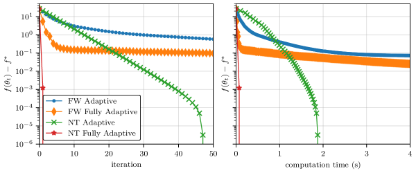
Figure 1. Convergence of Frank-Wolfe (FW) and Newton-type (NT) algorithm for the DRMPC problem ($N=10$) in terms of suboptimality gap as a function of iteration (top) and computation time (bottom).

In Figure 2, we compare the computation times required to solve the small scale DRMPC problem for difference horizon lengths $N$ via 1) the LMI optimization problem in 45 with MOSEK and 2) the NT algorithm. For $N\leq 5$, and therefore fewer variables and constraints, solving the DRMPC problem as an LMI optimization problem is faster. For $N>5$, however, solving the DRMPC problem as an LMI optimization problem becomes notably slower than using the NT algorithm. For $N\geq 15$, the computation time to solve the DRMPC problem as an LMI optimization problem is typically more than twice the computation time required for the Newton-type algorithm.

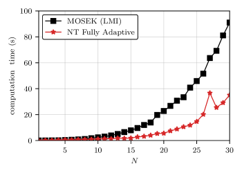
Figure 2. Comparison of computation times for the fully adaptive Newton-type (NT) algorithm and LMI formulation solved by MOSEK for the horizon $N$.

Closed-loop Performance

We initialize the state at $x(0)=\begin{bmatrix}1&1\end{bmatrix}^{\prime}$ and consider a fixed horizon of $N=10$. In the following discussion, we consider three different controllers: DRMPC with $d=(\varepsilon,\widehat{\Sigma})$, SMPC with $d=(0,\widehat{\Sigma})$, and RMPC with $d=(0,0)$.

To demonstrate the differences between the control laws for DRMPC, SMPC, and RMPC, we plot the first element of closed-loop state trajectory assuming the disturbance is zero, i.e., $w=0$, in Figure 3. RMPC drives the closed-loop state to the origin. SMPC, however, does not drive the closed-loop state to the origin even though the disturbance is zero. Since $u_{2}\geq 0$, the SMPC controller keeps $x_{1}$ slightly below the origin to mitigate the effect of positive values for $w_{2}$. The amount of offset is determined by the covariance of the disturbance. Since DRMPC considers a worst-case covariance for the disturbances, the offset is larger.

Thus, for $||\mathbf{w}_{\infty}||=0$, the closed-loop state for DRMPC (SMPC) does not converge to the origin. The origin is therefore not ISS for DRMPC (SMPC), despite satisfying Assumptions 2.1, 2.2, 3.1 and 3.2. By contrast, these assumptions are sufficient to render the origin ISS for the closed-loop system generated by RMPC [12, Thm. 23]. To summarize: SMPC and DRMPC are hedging against uncertainty and thereby giving up the deterministic properties of RMPC, such as ISS, in the pursuit of improved performance in terms of the expected value of the stage cost, i.e., $\mathcal{J}_{k}(\cdot)$.

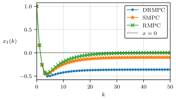
Figure 3. Closed-loop trajectories with zero disturbance, i.e., $x(k)=\phi_{d}(k;x,\mathbf{0})$, for the first element of the state, denoted $x_{1}(k)$.

We now investigate the performance of DRMPC relative to SMPC/RMPC for a distribution $\mathds{P}\in\mathcal{P}_{d}^{\infty}$. Specifically, we consider $w(k)$ to be i.i.d. in time and sampled from a zero-mean uniform distribution with a covariance of

$$\Sigma=\begin{bmatrix}0.01&0.01\\ 0.01&0.035\end{bmatrix}$$

We simulate $S=100$ different realizations of the disturbance trajectory for each controller. For each simulation $s\in\{1,\dots,S\}$, we define the closed-loop state and input trajectory $x^{s}(k)$ and $u^{s}(k)$, as well as the time-average stage cost

$$\mathcal{J}_{k}^{s}:=\frac{1}{k}\sum_{i=0}^{k-1}\ell(x^{s}(k),u^{s}(k))$$

In accordance with the results in Theorems 3.1 and 3.3, we consider the sample average approximations of $\mathbb{E}_{\mathds{P}}\left[|\phi(k;x,\mathbf{w}_{\infty})|\right]$ and $\mathcal{J}_{k}(x,d,\mathds{P})$ defined as

$$\tilde{\mathbb{E}}_{\mathds{P}}\left[|x(k)|^{2}\right]:=\frac{1}{S}\sum_{s=1}^{S}|x^{s}(k)|^{2}\qquad\tilde{\mathcal{J}}_{k}:=\frac{1}{S}\sum_{s=1}^{S}\mathcal{J}_{k}^{s}$$

In Figure 4, we plot $\tilde{\mathbb{E}}_{\mathds{P}}\left[|x(k)|^{2}\right]$ and $\tilde{\mathcal{J}}_{k}$. For each algorithm, we observe an initial, exponential decay in the mean-squared distance $\tilde{\mathbb{E}}_{\mathds{P}}\left[|x(k)|^{2}\right]$ towards a constant, but nonzero, value. These results for DRMPC are consistent with Corollary 3.3. We note, however, that DRMPC produces the largest value of $\tilde{\mathbb{E}}[|x(k)|^{2}]$, i.e., the mean-squared distance between the closed-loop state and the setpoint is larger for DRMPC than for SMPC or RMPC. While this result may initially seem counter-intuitive, the objective prescribed to the DRMPC problem is to minimize the expected value of the stage cost, not the expected distance to the origin. In terms of the expected value of the stage cost, i.e., $\tilde{\mathcal{J}}_{k}$, the performance of DRMPC is better than SMPC, which is better than RMPC. This difference becomes more pronounced as $k\rightarrow\infty$.

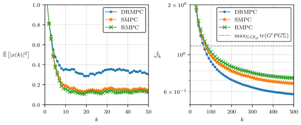
Figure 4. Sample averages of $\mathbb{E}_{\mathds{P}}\left[|\phi(k;x,\mathbf{w}_{\infty})|^{2}\right]$ and $\mathcal{J}_{k}(x,d,\mathds{P})$, denoted $\tilde{\mathbb{E}}_{\mathds{P}}\left[|x(k)|^{2}\right]$ and $\tilde{\mathcal{J}}_{k}$, for $S=100$ realizations of the closed-loop trajectory.

We note that $\Sigma\in\mathbb{B}_{d}$ in this example is intentionally chosen to exacerbate the effect of the disturbance on $x_{2}$ and thereby increase the cost of the closed-loop trajectory, i.e., a worst-case distribution. Therefore, DRMPC produces a superior control law relative to SMPC. If the ambiguity set, however, becomes too large relative to this value of $\Sigma$, the additional conservatism of DRMPC can produce worse performance than SMPC in terms of $\tilde{\mathcal{J}}_{k}$ for a fixed value of $\Sigma$. To demonstrate this tradeoff, we consider the same closed-loop simulation and plot the value of $\tilde{\mathcal{J}}_{T}$ at $T=500$ for various values of $\varepsilon$ and fixed $\widehat{\Sigma}$. In Figure 5, we observe that $\varepsilon\approx 0.11$ achieves the minimum value of $\mathcal{J}_{T}$, with an approximately 13% decrease in the value of $\tilde{\mathcal{J}}_{T}$ compared to $\varepsilon=0.01$. For values of $\varepsilon>0.11$, the value of $\tilde{\mathcal{J}}_{T}$ increases significantly until leveling off around $\varepsilon=1$. For large values of $\varepsilon$, DRMPC is too conservative because $\Sigma$ is now well within the interior of $\mathbb{B}_{d}$.

Another interesting feature in Figure 5 is that the range of values for $\mathcal{J}_{T}^{s}$ for each $s\in\{1,\dots,30\}$, shown by the shaded region, decreases as $\varepsilon$ increases. This behavior might also be explained by the increased conservatism of DRMPC as $\varepsilon$ increases. As the value of $\varepsilon$ increase, DRMPC generates a closed-loop system that is distributionally robust to a range of possible covariances. In this case, we might expect DRMPC to drive the closed-loop system to an operating region that attenuates the effect of all disturbances on the closed-loop cost at the expense of nominal performance. Thus, the closed-loop system becomes less sensitive to disturbances and thereby decreases the variability in performance at the expense of an increase in average performance. In summary, we are left with the classic trade-off in robust controller design; If we choose $\varepsilon$ too large, the excessively conservative DRMPC may perform worse than SMPC ($\varepsilon=0$). Thus, the design goal for DRMPC is to select a value of $\varepsilon$ that balances these two extremes.

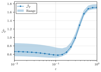
Figure 5. Sample average of the performance metric $\mathcal{J}_{T}(x,d,\mathds{P})$, denoted $\tilde{\mathcal{J}}_{T}$, for $T=500$ as a function of the ambiguity radius $\varepsilon$ for $S=30$ realizations of the disturbance trajectory. The shaded blue region indicates the range of values of $\tilde{\mathcal{J}}_{T}^{s}$ for $s\in\{1,\dots,30\}$.

6.2. Large scale example: Shell oil fractionator

To demonstrate the applicability of the Newton-type algorithm to control problems of an industrially relevant size, we now consider the Shell oil fractionator example in Maciejowski [18, s. 9.1] with $n=20$ states, $m=3$ inputs, and $p=3$ outputs. We include two disturbances ($q=2$): the intermediate reflux duty and the upper reflux duty. We assume these disturbances are i.i.d. and zero mean. We also note that $A$ in this problem is Schur stable.

We consider the input constraints $\mathbb{U}:=\left\{u\in\mathbb{R}^{3}\mid|u|_{\infty}\leq 1,\ u_{3}\geq 0\right\}$ in which the origin is again on the boundary of the input constraint $\mathbb{U}$. The disturbance set is $\mathbb{W}:=\{w\in\mathbb{R}^{2}\mid|w|_{\infty}\leq 1\}$ with the nominal covariance $\widehat{\Sigma}=0.01I_{2}$ and ambiguity an radius of $\varepsilon=0.1$. The outputs $y$ satisfy $y=Cx$ and we define cost matrices as $Q=C^{\prime}Q_{y}C$ and $R=0.1I_{3}$ in which $Q_{y}=\textnormal{diag}([20,\ 10,\ 1])$. We then define the terminal cost matrix $P\succ 0$ as the solution to the Lyapunov equation $A^{\prime}PA-P=-Q$. This DRMPC problem formulation satisfies Assumptions 2.1, 2.2 and 3.1 and $(A,Q^{1/2})$ is detectable (See Remark 3.1).

We initialize the state at $x(0)=0$ and use $N=10$. We consider the performance of the closed-loop system in which $w(k)$ is sampled from a zero-mean uniform distribution with a covariance of $\Sigma=\textnormal{diag}([0.04,\ 0.01])$. Note that $\Sigma\in\mathbb{B}_{d}$. We simulate $T=500$ time steps for $S=30$ realizations of the disturbance trajectory. We plot $\tilde{\mathcal{J}}_{k}$ in Figure 6 for DRMPC, SMPC, and RMPC. At $T=500$, we observe an almost negligible 0.2% decrease in $\tilde{\mathcal{J}}_{T}$ for DRMPC relative to SMPC. Longer horizons may increase this difference, but we expect the overall benefit of DRMPC to remain small and therefore not worth the extra computational demand.

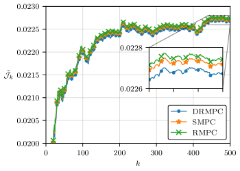
Figure 6. Sample average of $\mathcal{J}_{k}(x,d,\mathds{P})$, denoted $\widehat{\mathcal{J}}_{k}$, for $S=30$ realizations of the closed-loop trajectory.

Appendix A Additional technical proofs and results

Proof of Lemma 2.1.

From Goulart [11, Thm. 3.5] we have that $\Pi(x)$ is closed and convex for all $x\in\mathcal{X}$ and $\mathcal{X}$ is closed and convex. We now establish that $\Pi(x)$ is bounded. If $(\mathbf{M},\mathbf{v})\in\Pi(x)$, then $\mathbf{M}\mathbf{w}+\mathbf{v}\in\mathbb{U}^{N}$ for all $\mathbf{w}\in\mathbb{W}^{N}$. Since $0\in\mathbb{W}$, we have that for any $(\mathbf{M},\mathbf{v})\in\Pi(x)$, $\mathbf{v}$ must satisfy $\mathbf{v}\in\mathbb{U}^{N}$ Moreover, since the origin is in the interior of $\mathbb{W}$, there exists $\delta>0$ such that $B_{\delta}:=\{\mathbf{w}\in\mathbb{R}^{Nq}\mid|\mathbf{w}|\leq\delta\}\subseteq\mathbb{W}$. Since $\mathbb{U}$ is bounded, there exists $b\geq 0$, such that $|\mathbf{u}|\leq b$ for all $\mathbf{u}\in\mathbb{U}^{N}$. For any $(\mathbf{M},\mathbf{v})\in\Pi(x)$, we have

$$|\mathbf{M}\mathbf{w}|\leq 2b\quad\forall\ \mathbf{w}\in B_{\delta}$$ (57)

because $\mathbf{v}\in\mathbb{U}^{N}$. We have that 57 is equivalent to

$$\lVert\mathbf{M}\rVert_{2}:=\sup\left\{|\mathbf{M}\mathbf{w}|\ \middle|\ |\mathbf{w}|\leq 1\right\}\leq 2b/\delta$$

and we can construct a bounded set for $\mathbf{M}$ as follows:

$$\mathbf{M}\in\mathbb{M}:=\left\{\mathbf{M}\in\mathbb{R}^{Nm\times Nq}\ \middle|\ ||\mathbf{M}||_{2}\leq 2b/\delta\right\}$$

for all $(\mathbf{M},\mathbf{v})\in\Pi(x)$. Therefore, $(\mathbf{M},\mathbf{v})\in\Pi(x)\subseteq\mathbb{M}\times\mathbb{U}^{N}$ for all $x\in\mathcal{X}$. Since $\mathbb{U}$ and $\mathbb{M}$ are bounded, $\Pi(x)$ is bounded as well, uniformly for all $x\in\mathcal{X}$. ∎

Lemma A.1.

If $\mathbb{W}$ is bounded, then $\mathcal{D}$ is bounded.

Proof.

Define the set $\mathbb{S}:=\{\Sigma=\mathbb{E}_{\mathds{P}}\left[ww^{\prime}\right]\mid\mathds{P}\in\mathcal{M}(\mathbb{W})\}$ and note that $\mathbb{S}$ is bounded because $\mathbb{W}$ is bounded. By definition, $\mathbb{B}_{d}\subseteq\mathbb{S}$ for all $d\in\mathcal{D}$. Since $\widehat{\Sigma}\in\mathbb{B}_{d}$ for all $d=(\varepsilon,\widehat{\Sigma})$, then $\widehat{\Sigma}\in\mathbb{S}$ for all $d\in\mathcal{D}$ and therefore $\mathcal{D}\subseteq\mathbb{R}_{\geq 0}\times\mathbb{S}$.

Define $\rho:=\sup_{\Sigma\in\mathbb{S}}\textnormal{tr}(\Sigma)^{1/2}<\infty$. Therefore, $\mathbb{S}=\mathbb{B}_{(\rho,0)}$. Choose any $\widehat{\Sigma}\in\mathbb{S}$. If $\Sigma\in\mathbb{B}_{(\rho,0)}$, then

$$\textnormal{tr}\left(\widehat{\Sigma}+\Sigma-2\left(\widehat{\Sigma}^{1/2}\Sigma\widehat{\Sigma}^{1/2}\right)^{1/2}\right)\leq\textnormal{tr}\left(\widehat{\Sigma}\right)+\textnormal{tr}\left(\Sigma\right)\leq 2\rho$$

and therefore $\Sigma\in\mathbb{B}_{(2\rho,\hat{\Sigma})}$. Thus, $\mathbb{S}\subseteq\mathbb{B}_{(\rho,0)}\subseteq\mathbb{B}_{(2\rho,\hat{\Sigma})}$. For all $(\varepsilon,\widehat{\Sigma})\in\mathcal{D}$, we have $\mathbb{B}_{(\varepsilon,\widehat{\Sigma})}\subseteq\mathbb{S}\subseteq\mathbb{B}_{(2\rho,\hat{\Sigma})}$ and therefore $\varepsilon\leq 2\rho$. Hence, $\mathcal{D}\subseteq[0,2\rho]\times\mathbb{S}$ and $\mathcal{D}$ is bounded. ∎

Appendix B Optimal terminal cost

Since the term $\textnormal{tr}(G^{\prime}PG\Sigma)$ appears on the right-hand side of all bounds in Theorems 3.1, 3.2 and 3.3, a straightforward design strategy for DRMPC is to select the value of $P$ that minimizes this term subject to the constraints in Assumption 3.1. In the following lemma, we show that the value of $P$ that achieves this goal is given by 19 in Assumption 3.3.

Lemma B.1 (Optimal terminal cost).

For any $Q,R\succ 0$, a solution to

$$\inf_{P\succ 0,K_{f}}\ \textnormal{tr}(G^{\prime}PG\Sigma)$$

s.t. $$P-Q-K_{f}^{\prime}RK_{f}\succeq(A+BK_{f})^{\prime}P(A+BK_{f})$$

is given by the solution to the DARE 19 and the associated controller $K_{f}:=-(R+B^{\prime}PB)B^{\prime}PA$ for all $G\in\mathbb{R}^{m\times q}$ and $\Sigma\succeq 0$.

Lemma B.1 suggests that, if possible, one should always select $P$ according to Assumption 3.3 to minimize the value of $\textnormal{tr}(G^{\prime}PG\Sigma)$ for all $\Sigma\succeq 0$. Therefore, Assumption 3.3, in addition to being a convenient and common method to select $P$, also produces the best theoretical bound for the performance of the closed-loop system.

Proof of Lemma B.1.

Consider the unique solution $P^{*}\succ 0$ that satisfies 19 and choose any $G\in\mathbb{R}^{m\times q}$ and $\Sigma\succeq 0$. We denote $D:=G\Sigma G^{\prime}$ and note that $D\succeq 0$. We consider the equivalent optimization problem

$$\inf_{K_{f},S}\ \textnormal{tr}((P^{*}-S)D)$$ (58a)

s.t. $$P^{*}-S-Q-K_{f}^{\prime}RK_{f}\succeq(A+BK_{f})^{\prime}(P^{*}-S)(A+BK_{f})$$ (58b)

$$P^{*}-S\succ 0,\quad S\succeq 0$$ (58c)

If the solution to this optimization problem is $S=0$ for all $D\succeq 0$, then $P^{*}$ must be a solution to the original optimization problem.

We now prove that $S=0$. Assume $K_{f}\in\mathbb{R}^{m\times n}$ and $S\succeq 0$ exist such that 58b and 58c hold. Note that this inequality implies that $A+BK_{f}$ is Schur stable. Since $P^{*}$ defines the optimal cost of the infinite horizon unconstrained LQR problem, any $K_{f}\in\mathbb{R}^{m\times n}$ must satisfy

$$(A+BK_{f})^{\prime}(P^{*})(A+BK_{f})\succeq P^{*}-Q-K_{f}^{\prime}RK_{f}$$ (59)

By combining 58b and 59, we have that $K_{f}$ and $S\succeq 0$ must satisfy

$$(A+BK_{f})^{\prime}S(A+BK_{f})\succeq S$$ (60)

However, if there exists $S\neq 0$ satisfying 60 with $S\succeq 0$, then $A+BK_{f}$ is not Schur stable. Since $A+BK_{f}$ is Schur stable, the only value of $S\succeq 0$ that satisfies 60 is $S=0$. Therefore, $S=0$ is the only solution to the modified optimization problem and $P^{*}$ is the solution to the original optimization problem. Note that since the choices of $G\in\mathbb{R}^{m\times q}$ and $\Sigma\succeq 0$ were arbitrary, this solution holds for any $G\in\mathbb{R}^{m\times q}$ and $\Sigma\succeq 0$. ∎

Appendix C Fundamental mathematical properties of DRMPC formulation

We now establish some fundamental mathmatical properties of 13 to ensure that subsequently defined quantities are indeed well-defined.

We first introduce some notation and definitions. A function $f:X\rightarrow\mathbb{R}$ is lower semincontinuous if $\liminf_{x\rightarrow x_{0}}f(x)\geq f(x_{0})$ for all $x_{0}\in X$. Let $\mathcal{B}(\Omega)$ denote the Borel field of some set $\Omega$, i.e., the subsets of $\Omega$ generated through relative complements and countable unions of all open subsets of $\Omega$. For the metric spaces $X$ and $Y$, a function $f:X\rightarrow Y$ is Borel measurable if for each open set $O\subseteq Y$, we have $f^{-1}(O):=\{x\in X\mid f(x)\in O\}\in\mathcal{B}(X)$. For the metric spaces $X$ and $Y$, a set-valued mapping $F:X\rightrightarrows Y$ is Borel measurable if for every open set $O\subseteq Y$, we have $F^{-1}(O):=\{x\in X\mid F(x)\cap O\neq\emptyset\}\in\mathcal{B}(X)$ [31, Def. 14.1].

Proposition C.1 (Existence and measurability).

If Assumptions 2.1 and 2.2 hold, then for all $d\in\mathcal{D}$, $V_{d}:\mathcal{X}\times\Theta\rightarrow\mathbb{R}_{\geq 0}$ is convex and continuous, $V_{d}^{0}:\mathcal{X}\rightarrow\mathbb{R}_{\geq 0}$ is convex and lower semicontinuous, $\theta^{0}:\mathcal{X}\rightrightarrows\Theta$ is Borel measurable, and $\theta^{0}_{d}(x)\neq\emptyset$ for all $x\in\mathcal{X}$.

Proof.

We have that $L(\cdot)$ is continuous and $\mathbb{B}_{d}^{N}$ is compact [27, Lemma A.6]. Therefore, $V_{d}(x,\theta)$ is continuous for all $(x,\theta)\in\mathbb{R}^{n}\times\Theta$ [30, Thm. C.28]. We also have that $L(x,\theta,\boldsymbol{\Sigma})$ is convex in $(x,\theta)\in\mathbb{R}^{n}\times\Theta$ for all $\boldsymbol{\Sigma}\in\mathbb{B}_{d}^{N}$. From Danskin’s theorem, we have that $V_{d}(x,\theta)$ is also convex. Since $V_{d}(x,\theta)$ is continuous and $\Pi(x)$ is compact for each $x\in\mathcal{X}$, we have that $\theta^{0}_{d}(x)\neq\emptyset$, i.e., the minimum is attained, for all $x\in\mathcal{X}$. Since $\mathbb{Z}$ and $\mathbb{X}_{f}$ are closed, we have that

$$\mathcal{Z}:=\bigcap_{\mathbf{w}\in\mathbb{W}^{N}}\left\{(x,\mathbf{M},\mathbf{v})\in\mathbb{R}^{n}\times\Theta\ \middle|\ \begin{matrix}\mathbf{x}=\mathbf{A}x+\mathbf{B}\mathbf{v}+(\mathbf{B}\mathbf{M}+\mathbf{G})\mathbf{w}\\ \mathbf{u}=\mathbf{M}\mathbf{w}+\mathbf{v}\\ (x(k),u(k))\in\mathbb{Z}\ \forall\ k\in\mathbb{I}_{0:N-1}\\ x(N)\in\mathbb{X}_{f}\end{matrix}\right\}$$

is also closed. From the Proof of Lemma 2.1, we have that $\mathcal{Z}\subseteq\mathbb{R}^{n}\times(\mathbb{M}\times\mathbb{U})$ in which $\mathbb{U}$ and $\mathbb{M}$ are compact. Therefore,

$$V^{0}_{d}(x)=\min_{\theta}\left\{V_{d}(x,\theta)\mid(x,\theta)\in\mathcal{Z}\right\}\quad\text{and}\quad\theta^{0}_{d}(x)=\arg\min_{\theta}\left\{V_{d}(x,\theta)\mid(x,\theta)\in\mathcal{Z}\right\}$$

From Bertsekas and Shreve [4, Prop. 7.33], we have that $V_{d}^{0}:\mathcal{X}\rightarrow\mathbb{R}_{\geq 0}$ is lower semicontinuous and $\theta^{0}:\mathcal{X}\rightrightarrows\Theta$ is Borel measurable. ∎

Since $\theta^{0}_{d}(x)$ is Borel measurable and $\mathbb{U}$ is compact, we have from Proposition C.1 and [4, Lemma 7.18] that there exists a selection rule such that $\kappa_{d}:\mathcal{X}\rightarrow\mathbb{U}$ is also Borel measurable. Thus, the closed-loop system $\phi(k;x,\mathbf{w}_{\infty})$ is measurable with respect to $\mathbf{w}_{\infty}$ for all $k\geq 0$. Moreover, all probabilities and expected values for the closed-loop system $\phi(\cdot)$ are well defined.

We also have the following corollary to Proposition C.1 if $\mathbb{Z}$, $\mathbb{X}_{f}$, and $\mathbb{W}$ are polytopes.

Corollary C.1 (Continuity of optimal value function).

If Assumptions 2.1 and 2.2 hold and $\mathbb{Z},\mathbb{X}_{f},\mathbb{W}$ are polyhedral, then for all $d\in\mathcal{D}$, $V^{0}_{d}:\mathcal{X}\rightarrow\mathbb{R}_{\geq 0}$ is continuous.

Proof.

Since $\mathbb{Z},\mathbb{X}_{f},\mathbb{W}$ are polyhedral, we have from Goulart [11, Cor. 3.8] $\mathcal{X}$ is polyhedral. From the Proof of Lemma 2.1, we have that $\mathcal{Z}\subseteq\mathbb{R}^{n}\times(\mathbb{M}\times\mathbb{U})$ in which $\mathbb{U}$ and $\mathbb{M}$ are bounded. Recall from the Proof of Proposition C.1 that $V_{d}:\mathbb{R}^{n}\times\Theta\rightarrow\mathbb{R}^{n}$ is continuous. Therefore,

$$V^{0}_{d}(x)=\min_{\theta}\left\{V_{d}(x,\theta)\mid(x,\theta)\in\mathcal{Z}\right\}\quad\text{and}\quad\theta^{0}_{d}(x)=\arg\min_{\theta}\left\{V_{d}(x,\theta)\mid(x,\theta)\in\mathcal{Z}\right\}$$

From Rawlings et al. [30, Thm. C.34], we have that $V^{0}_{d}:\mathcal{X}\rightarrow\mathbb{R}$ is continuous and $\theta^{0}_{d}:\mathcal{X}\rightrightarrows\Theta$ is outer semicontinuous. ∎

References

- Allan et al. [2017] D. A. Allan, C. N. Bates, M. J. Risbeck, and J. B. Rawlings. On the inherent robustness of optimal and suboptimal nonlinear MPC. Sys. Cont. Let., 106:68 – 78, 2017. ISSN 0167-6911. doi: 10.1016/j.sysconle.2017.03.005.
- ApS [2022] M. ApS. The MOSEK optimization toolbox for MATLAB manual. Version 10.0., 2022. URL http://docs.mosek.com/9.0/toolbox/index.html.
- Bertsekas [2009] D. Bertsekas. Convex optimization theory, volume 1. Athena Scientific, 2009.
- Bertsekas and Shreve [1996] D. Bertsekas and S. E. Shreve. Stochastic optimal control: the discrete-time case, volume 5. Athena Scientific, 1996.
- Cannon et al. [2009] M. Cannon, B. Kouvaritakis, and X. Wu. Probabilistic constrained mpc for multiplicative and additive stochastic uncertainty. IEEE Transactions on Automatic Control, 54(7):1626–1632, 2009.
- Coppens and Patrinos [2021] P. Coppens and P. Patrinos. Data-driven distributionally robust mpc for constrained stochastic systems. IEEE Control Systems Letters, 6:1274–1279, 2021.
- Coulson et al. [2021] J. Coulson, J. Lygeros, and F. Dörfler. Distributionally robust chance constrained data-enabled predictive control. IEEE Transactions on Automatic Control, 67(7):3289–3304, 2021.
- Farina et al. [2016] M. Farina, L. Giulioni, and R. Scattolini. Stochastic linear model predictive control with chance constraints–a review. Journal of Process Control, 44:53–67, 2016.
- Fochesato and Lygeros [2022] M. Fochesato and J. Lygeros. Data-driven distributionally robust bounds for stochastic model predictive control. In 61st Conference on Decision and Control (CDC 2022), 2022.
- Gelbrich [1990] M. Gelbrich. On a formula for the l2 wasserstein metric between measures on euclidean and hilbert spaces. Mathematische Nachrichten, 147(1):185–203, 1990.
- Goulart [2007] P. J. Goulart. Affine feedback policies for robust control with constraints. PhD thesis, University of Cambridge, 2007.
- Goulart et al. [2006] P. J. Goulart, E. C. Kerrigan, and J. M. Maciejowski. Optimization over state feedback policies for robust control with constraints. Automatica, 42:523–533, 2006.
- Grimm et al. [2004] G. Grimm, M. J. Messina, S. E. Tuna, and A. R. Teel. Examples when nonlinear model predictive control is nonrobust. Automatica, 40:1729–1738, 2004.
- Hewing et al. [2020] L. Hewing, K. P. Wabersich, and M. N. Zeilinger. Recursively feasible stochastic model predictive control using indirect feedback. Automatica, 119:109095, 2020.
- Kuhn et al. [2019] D. Kuhn, P. M. Esfahani, V. A. Nguyen, and S. Shafieezadeh-Abadeh. Wasserstein distributionally robust optimization: Theory and applications in machine learning. In Operations research & management science in the age of analytics, pages 130–166. Informs, 2019.
- Li et al. [2021] B. Li, Y. Tan, A.-G. Wu, and G.-R. Duan. A distributionally robust optimization based method for stochastic model predictive control. IEEE Transactions on Automatic Control, 2021.
- Lorenzen et al. [2016] M. Lorenzen, F. Dabbene, R. Tempo, and F. Allgöwer. Constraint-tightening and stability in stochastic model predictive control. IEEE Transactions on Automatic Control, 62(7):3165–3177, 2016.
- Maciejowski [2001] J. M. Maciejowski. Predictive Control with Constraints. Pearson Education, 2001.
- Mark and Liu [2020] C. Mark and S. Liu. Stochastic mpc with distributionally robust chance constraints. IFAC-PapersOnLine, 53(2):7136–7141, 2020.
- Mark and Liu [2022] C. Mark and S. Liu. Recursively feasible data-driven distributionally robust model predictive control with additive disturbances. IEEE Control Systems Letters, 7:526–531, 2022.
- Mayne et al. [2005] D. Q. Mayne, M. M. Seron, and S. Raković. Robust model predictive control of constrained linear systems with bounded disturbances. Automatica, 41(2):219–224, 2005.
- McAllister and Rawlings [2023] R. D. McAllister and J. B. Rawlings. On the inherent distributional robustness of stochastic and nominal model predictive control. IEEE Transactions on Automatic Control, 2023.
- Mesbah [2016] A. Mesbah. Stochastic model predictive control: An overview and perspectives for future research. IEEE Control Systems Magazine, 36(6):30–44, 2016.
- Micheli et al. [2022] F. Micheli, T. Summers, and J. Lygeros. Data-driven distributionally robust mpc for systems with uncertain dynamics for systems with uncertain dynamics. In 61st IEEE Conference on Decision and Control (CDC 2022), 2022.
- Munoz-Carpintero and Cannon [2020] D. Munoz-Carpintero and M. Cannon. Convergence of stochastic nonlinear systems and implications for stochastic model-predictive control. IEEE Transactions on Automatic Control, 66(6):2832–2839, 2020.
- Nguyen et al. [2022] V. A. Nguyen, D. Kuhn, and P. Mohajerin Esfahani. Distributionally robust inverse covariance estimation: The Wasserstein shrinkage estimator. Operations Research, 70(1):490–515, 2022.
- Nguyen et al. [2023] V. A. Nguyen, S. Shafieezadeh-Abadeh, D. Kuhn, and P. Mohajerin Esfahani. Bridging bayesian and minimax mean square error estimation via wasserstein distributionally robust optimization. Mathematics of Operations Research, 48(1):1–37, 2023.
- Pan and Faulwasser [2023] G. Pan and T. Faulwasser. Distributionally robust uncertainty quantification via data-driven stochastic optimal control. arXiv preprint arXiv:2306.02318, 2023.
- Pedregosa et al. [2020] F. Pedregosa, G. Negiar, A. Askari, and M. Jaggi. Linearly convergent frank-wolfe with backtracking line-search. In International conference on artificial intelligence and statistics, pages 1–10. PMLR, 2020.
- Rawlings et al. [2020] J. B. Rawlings, D. Q. Mayne, and M. Diehl. Model predictive control: theory, computation, and design. Nob Hill Publishing Madison, WI, 2020.
- Rockafellar and Wets [2009] R. T. Rockafellar and R. J.-B. Wets. Variational analysis, volume 317. Springer Science & Business Media, 2009.
- Sheriff and Mohajerin Esfahani [2023] M. R. Sheriff and P. Mohajerin Esfahani. Nonlinear distributionally robust optimization. arXiv preprint arXiv:2306.03202, 2023.
- Stellato et al. [2020] B. Stellato, G. Banjac, P. Goulart, A. Bemporad, and S. Boyd. OSQP: an operator splitting solver for quadratic programs. Mathematical Programming Computation, 12(4):637–672, 2020. doi: 10.1007/s12532-020-00179-2. URL https://doi.org/10.1007/s12532-020-00179-2.
- Tan et al. [2022] Y. Tan, J. Yang, W.-H. Chen, and S. Li. A distributionally robust optimization approach to two-sided chance constrained stochastic model predictive control with unknown noise distribution. arXiv preprint arXiv:2203.08457, 2022.
- Taşkesen et al. [2023] B. Taşkesen, D. A. Iancu, Ç. Koçyiğit, and D. Kuhn. Distributionally robust linear quadratic control. arXiv preprint arXiv:2305.17037, 2023.
- Van Parys et al. [2015] B. P. Van Parys, D. Kuhn, P. J. Goulart, and M. Morari. Distributionally robust control of constrained stochastic systems. IEEE Transactions on Automatic Control, 61(2):430–442, 2015.
- Yu et al. [2014] S. Yu, M. Reble, H. Chen, and F. Allgöwer. Inherent robustness properties of quasi-infinite horizon nonlinear model predictive control. Automatica, 50(9):2269 – 2280, 2014. ISSN 0005-1098. doi: 10.1016/j.automatica.2014.07.014.