Bordifications of the moduli spaces of tropical curves and abelian varieties, and unstable cohomology of $\mathrm{GL}_{g}(\mathbb{Z})$ and $\mathrm{SL}_{g}(\mathbb{Z})$

Abstract.

We construct bordifications of the moduli spaces of tropical curves and of tropical abelian varieties, and show that the tropical Torelli map extends to their bordifications. We prove that the classical bi-invariant differential forms studied by Cartan extend to these bordifications by studying their behaviour at infinity, and consequently deduce infinitely many new non-zero unstable cohomology classes in the cohomology of the general and special linear groups $\mathrm{GL}_{g}(\mathbb{Z})$ and $\mathrm{SL}_{g}(\mathbb{Z})$. In addition, we completely determine the cohomology of the link of the moduli space of tropical abelian varieties within a certain range, and show that it contains the stable cohomology of the general linear group. In the process, we define new transcendental invariants associated to the minimal vectors of quadratic forms. We also show that a certain part of the cohomology of the general linear group $\mathrm{GL}_{g}(\mathbb{Z})$ admits the structure of a motive.

1. Introduction

The main goal of this paper is an algebro-geometric construction of bordifications of the moduli spaces of tropical curves and abelian varieties. Before describing these in detail, we first present some applications to the cohomology of the special and general linear groups.

1.1. Unstable cohomology of linear groups

Let $\mathcal{P}_{g}$ denote the space of symmetric positive definite $g\times g$ matrices $X$ with real entries. It is a connected contractible space equipped with a right action of $h\in\mathrm{GL}_{g}(\mathbb{R})$ via the map $h(X)=h^{T}Xh$.

Since the orbifold $\mathcal{P}_{g}/\mathrm{GL}_{g}(\mathbb{Z})$ is a $K(\pi,1)$ one has $H^{n}(\mathrm{GL}_{g}(\mathbb{Z});\mathbb{R})=H^{n}(\mathcal{P}_{g}/\mathrm{GL}_{g}(\mathbb{Z});\mathbb{R})$. Block direct sum of matrices $X\mapsto X\oplus 1$ defines a map $\mathcal{P}_{g}\rightarrow\mathcal{P}_{g+1}$. The stable cohomology is defined to be the limit with respect to these maps:

$$H^{n}(\mathrm{GL}_{\infty}(\mathbb{Z});\mathbb{R})=\varprojlim_{g}H^{n}(\mathrm{GL}_{g}(\mathbb{Z});\mathbb{R})\ .$$

It was famously computed by Borel [Bor74], from which he deduced the ranks of the rational algebraic $K$-theory of the integers (and, more generally, of all number fields), which is of fundamental importance in the modern theory of motives. Very little is known about the unstable cohomology of the groups $\mathrm{SL}_{g}(\mathbb{Z})$ and $\mathrm{GL}_{g}(\mathbb{Z})$. See figures 1 and 3 for the range in which their cohomology groups are completely known.

$$\begin{array}[]{c|cccccccccccccccccc}g&H^{i}(\mathrm{GL}_{g}(\mathbb{Z}))\\ \hline\cr 2&H^{0}\\ 3&H^{0}\\ 4&H^{0}\\ 5&H^{0}&&&H^{5}&\\ 6&H^{0}&&&H^{5}&&\framebox{$H^{8}$}\\ 7&H^{0}&&&H^{5}&&&H^{9}&&&&&H^{14}&\framebox{$H^{15}$}\\ \end{array}$$

Figure 1. Known ranges for which the cohomology of $\mathrm{GL}_{g}(\mathbb{Z})$ has been completely determined [Sou78, LS78, Ash84, EVGS13]. An entry $H^{i}$ in the table indicates that $H^{i}(\mathrm{GL}_{g}(\mathbb{Z});\mathbb{R})$ is non-zero and of rank $1$. All non-zero classes are explained by theorem 1.1 except for the two boxed entries.

Even less is known about the cohomology with compact supports $H_{c}^{n}(\mathcal{P}_{g}/\mathrm{GL}_{g}(\mathbb{Z});\mathbb{R})$, which we shall denote by $H_{c}^{n}(\mathrm{GL}_{g}(\mathbb{Z});\mathbb{R})$. The notation is justified by duality: indeed, when $g$ is odd, the orbifold $\mathcal{P}_{g}/\mathrm{GL}_{g}(\mathbb{Z})$ is orientable and its compactly supported cohomology is Poincaré dual to ordinary cohomology. However, in the case when $g$ is even, the cohomology with and without compact supports are a priori unrelated. There is no stability property for cohomology with compact supports, as one may see from figure 2.

The ordinary cohomology of the special linear group $\mathrm{SL}_{g}(\mathbb{Z})$ coincides with that of $\mathrm{GL}_{g}(\mathbb{Z})$ when $g$ is odd, but is built out of the cohomology of $\mathrm{GL}_{g}(\mathbb{Z})$ with and without compact supports in the case when $g$ is even. See figure 3 for a table of known results.

1.2. Cohomological results

Consider the abstract graded exterior algebra

$$\Omega_{\mathrm{can}}^{\bullet}=\bigwedge\bigoplus_{k\geq 1}\mathbb{Q}\,\omega^{4k+1}$$

with generators $\omega^{4k+1}$ in degree $4k+1$. Following Cartan, for any $X\in\mathcal{P}_{g}$ and $k>1$, let

(1.1) $$\omega^{4k+1}_{X}=\mathrm{tr}((X^{-1}dX))^{4k+1}\ ,$$

which is a well-defined closed differential form on $\mathcal{P}_{g}$ with a number of remarkable properties, including bi-invariance with respect to left and right multiplication by $\mathrm{GL}_{g}(\mathbb{R})$. Consequently, any $\omega\in\Omega_{\mathrm{can}}^{n}$ defines a closed differential form of degree $n$ on $\mathcal{P}_{g}/\mathrm{GL}_{g}(\mathbb{Z})$.

Consequently there is a natural map, which is sometimes referred to as either the ‘Borel map’ or ‘Matsushima homomorphism’:

(1.2) $$j:\Omega_{\mathrm{can}}^{n}\otimes_{\mathbb{Q}}\mathbb{R}\longrightarrow H^{n}(\mathrm{GL}_{g}(\mathbb{Z});\mathbb{R})\ .$$

Borel proved that $j$ is injective for $n\leq g/4$. Results of Matsushima [Mat62] and Garland [Gar71] imply that the map $j$ is surjective in the same range. Although this range is narrow, it nonetheless tends to infinity, which allowed Borel to compute the stable limit:

$$\Omega^{\bullet}_{\mathrm{can}}\otimes_{\mathbb{Q}}\mathbb{R}\cong H^{\bullet}(\mathrm{GL}_{\infty}(\mathbb{Z});\mathbb{R})\ .$$

$$\begin{array}[]{c|cccccccccccccccccc}g&\\ \hline\cr 2&\\ 3&H^{6}_{c}\\ 4&\quad H^{7}_{c}\\ 5&&&H^{10}_{c}&&&H^{15}_{c}\\ 6&&&\quad H^{11}_{c}&\framebox{$H^{12}_{c}$}&&\quad H^{16}_{c}\\ 7&&&&\quad\framebox{$H^{13}_{c}$}&H^{14}_{c}&&&&H^{19}_{c}&&H^{23}_{c}&&&H^{28}_{c}\\ \end{array}$$

Figure 2. Compactly-supported cohomology of $\mathcal{P}_{g}/\mathrm{GL}_{g}(\mathbb{Z})$ in the known ranges [Sou78, LS78, Ash84, EVGS13]. An entry $H_{c}^{i}$ in the table indicates that $H_{c}^{i}(\mathrm{GL}_{g}(\mathbb{Z});\mathbb{R})$ is non-zero and of rank $1$. All non-trivial classes are explained by theorem 1.1 except for the two boxed entries.

Let $g>1$ be odd, and let $\Omega(g)\subset\Omega_{\mathrm{can}}$ denote the graded subalgebra generated by $\omega^{5},\ldots,\omega^{2g-1}$. All forms $\omega^{n}$ of degree $n\geq 2g$ vanish identically on $\mathcal{P}_{g}$. In order to state our results, we divide $\Omega(g)$ into two subspaces. Let $\Omega_{c}(g)\subset\Omega(g)$ denote the ideal generated by $\omega^{2g-1}$. We shall call $\Omega_{c}(g)$ the space of forms of ‘compact type’ and define $\Omega_{nc}(g)\subset\Omega(g)$ to be the graded subalgebra generated by $1,\omega^{5},\ldots,\omega^{2g-5}$. The subscript $nc$ stands for ‘non-compact’ type. One has $\Omega(g)=\Omega_{c}(g)\oplus\Omega_{nc}(g)$.

Theorem 1.1.

Let $g>1$ be odd. There are injective maps

$$(i).\! \Omega^{\bullet}_{nc}(g)\otimes_{\mathbb{Q}}\mathbb{R}\hookrightarrow H^{\bullet}(\mathrm{GL}_{h}(\mathbb{Z});\mathbb{R})\quad\hbox{ for all }h\geq g\ ,$$

$$(ii). \Omega^{\bullet}_{c}(g)\otimes_{\mathbb{Q}}\mathbb{R}\hookrightarrow H_{c}^{\bullet+1}(\mathrm{GL}_{g}(\mathbb{Z});\mathbb{R})\ ,$$

$$(iii). \Omega^{\bullet}_{c}(g)\otimes_{\mathbb{Q}}\mathbb{R}\hookrightarrow H_{c}^{\bullet+2}(\mathrm{GL}_{g+1}(\mathbb{Z});\mathbb{R})\ .$$

These facts imply the following results about the special linear group:

$$(iv).\! \Omega^{\bullet}_{nc}(g)\otimes_{\mathbb{Q}}\mathbb{R}\hookrightarrow H^{\bullet}(\mathrm{SL}_{h}(\mathbb{Z});\mathbb{R})\quad\hbox{ for all }h\geq g\ ,$$

$$(v). (\Omega^{\bullet}_{nc}(g)\oplus\Omega^{d_{g+1}-\bullet-2}_{c}(g))\otimes_{\mathbb{Q}}\mathbb{R}\hookrightarrow H^{\bullet}(\mathrm{SL}_{g+1}(\mathbb{Z});\mathbb{R})\ .$$

Statement $(i)$ (and implicitly $(ii)$) is discussed in a research announcement of Ronnie Lee [Lee78], but no proof seems to have appeared in print. The statement also appears in Franke [Fra08], and is proven in a slightly weaker form in [Gro13], both using automorphic methods. Our proof bears some similarity to the strategy suggested by Lee and implies that the map $(i)$ for $h=g$ and $(ii)$ are canonically split: the key point is the construction of representatives for elements in $\Omega_{c}(g)$ which have compact support. Statement $(i)$ implies, but is much stronger than, Borel’s result on the injectivity of (1.2) in small degrees.

The statement $(iii)$ about the unstable cohomology of linear groups of even rank is new. It follows from a much stronger theorem (theorem 1.3 below) on the existence of cohomology classes in the moduli space of tropical abelian varieties and uses recent results on the acyclicity of the ‘inflation complex’ in [MBW22].

To illustrate the content of $(iv)$ and $(v)$, consider the following table of the known cohomology of $\mathrm{SL}_{g}(\mathbb{Z})$, taken from [CFP14] and based on computer calculations of [EVGS13].

$$\begin{array}[]{c|c|ccccccccccccccccc}g&\dim(\mathcal{P}_{g})&n=0&1&2&3&4&5&6&7&8&9&10&11&12&13&14&15\\ \hline\cr 2&3&1&\\ 3&6&1&\\ 4&10&1&&&1\\ 5&15&1&&&&&1\\ 6&21&1&&&&&2&&&\framebox{1}&\framebox{1}&1\\ 7&28&1&&&&&1&&&&1&&&&&1&\framebox{1}\\ \end{array}$$

Figure 3. An entry in row $g$ and column $n$ equals $\dim H^{n}(\mathrm{SL}_{g}(\mathbb{Z});\mathbb{R})$; blank entries are zero. All non-zero entries in this table are explained by the previous theorem except for the three boxed entries. Two of them would in fact follow from our results above, together with another theorem announced by Lee. Indeed, the class in $H^{9}(\mathrm{SL}_{6}(\mathbb{Z});\mathbb{R})$, which corresponds to a class in $H^{12}_{c}(\mathrm{GL}_{6}(\mathbb{Z});\mathbb{R})$, is denoted by $[\omega^{5}|\omega^{5}]$ in Lee’s notation. The class in $H^{15}(\mathrm{SL}_{7}(\mathbb{Z});\mathbb{R})$ corresponds to a class in $H^{13}_{c}(\mathrm{GL}_{7}(\mathbb{Z});\mathbb{R})$ which should be related to it by the inflation map of [MBW22].

Only the boxed class in $H^{8}(\mathrm{SL}_{6}(\mathbb{Z});\mathbb{R})$, which comes from a class in $H^{8}(\mathrm{GL}_{6}(\mathbb{Z});\mathbb{R})$, is unexplained. Its dual homology class lies in $H_{8}(\mathrm{GL}_{6}(\mathbb{Z});\mathbb{R})$, and is possibly proportional to the image of the second Morita class in $H_{8}(\mathrm{Out}(F_{6}))$ under the Jacobian map. It is not known if this image is zero or not. It was proven by Bismut and Lott [BL97] that for $g>1$ odd, the class of $\omega^{2g-1}$ in $H^{2g-1}(\mathrm{GL}_{g}(\mathbb{Z}))$ vanishes. Conjecture 5.3 in [MSS16] states that the class of $\omega^{2g-1}$ also vanishes in $H^{2g-1}(\mathrm{GL}_{g+1}(\mathbb{Z}))$. Cuspidal classes in the cohomology of $\mathrm{GL}_{n}(\mathbb{Z})$ were constructed for the first time in [BCG23].

1.3. Moduli of tropical abelian varieties

Theorem 1.1 is a consequence of a stronger result concerning cohomology classes on the link $\left|L\mathcal{A}_{g}^{\mathrm{trop}}\right|$ of the moduli space of tropical abelian varieties, which we presently explain. The reason for the vertical bar notation is that $\left|L\mathcal{A}_{g}^{\mathrm{trop}}\right|$ is merely the topological incarnation of a richer kind of hybrid geometric object, denoted by $L\mathcal{A}_{g}^{\mathrm{trop}}$, which we shall discus later. In any case, as a set, $\left|L\mathcal{A}_{g}^{\mathrm{trop}}\right|$ is the quotient of the rational closure $\mathcal{P}^{\mathrm{rt}}_{g}$ of $\mathcal{P}_{g}$ consisting of positive semi-definite matrices with rational kernel, modulo the action of $\mathrm{GL}_{g}(\mathbb{Z})$, and by $\mathbb{R}^{\times}$ acting by scalar multiplication. We consider its decomposition into perfect cones, due to Voronoï [Vor08, Mar03], which are described as follows. Let $Q$ be a positive definite quadratic form, and let

$$M_{Q}=\{\lambda\in\mathbb{Z}^{g}\backslash\{0\}:Q(\lambda)\leq Q(\mu)\quad\hbox{for all }\mu\in\mathbb{Z}^{g}\backslash\{0\}\}$$

denote the set of minimal vectors of $Q$. The set of $\lambda\lambda^{T}$, for $\lambda\in M_{Q}$, span a convex polyhedral cone $\sigma_{Q}$ in the link $L\mathcal{P}^{\mathrm{rt}}_{g}$ of $\mathcal{P}^{\mathrm{rt}}_{g}$, whose points are projective classes of symmetric matrices. The topological space $\left|L\mathcal{A}_{g}^{\mathrm{trop}}\right|$ is obtained by gluing together $\mathrm{GL}_{g}(\mathbb{Z})$-equivalence classes of quotients $\sigma_{Q}/\mathrm{Aut}(\sigma_{Q})$ of polyhedral cones by their finite groups of automorphisms.

Examples 1.2.

(See figure 4). The quadratic form $Q(x_{1},x_{2})=x_{1}^{2}+x_{1}x_{2}+x_{2}^{2}$ has minimal vectors $M_{Q}=\{(\pm 1,0),(0,\pm 1),\pm(1,-1)\}$, and hence

$$\sigma_{Q}=\left\{\begin{pmatrix}\alpha_{1}+\alpha_{3}&-\alpha_{3}\\ -\alpha_{3}&\alpha_{2}+\alpha_{3}\end{pmatrix}:\alpha_{1},\alpha_{2},\alpha_{3}\geq 0\right\}$$

is the convex hull of the rank 1 matrices $\left(\begin{smallmatrix}1&0\\ 0&0\end{smallmatrix}\right)$, $\left(\begin{smallmatrix}0&0\\ 0&1\end{smallmatrix}\right)$, $\left(\begin{smallmatrix}1&-1\\ -1&1\end{smallmatrix}\right)$. There is a single $\mathrm{GL}_{2}(\mathbb{Z})$-orbit of cells of maximal dimension in $|L\mathcal{A}_{2}^{\mathrm{trop}}|$ generated by $\sigma_{Q}$. The stabiliser of $\sigma_{Q}$ is the symmetric group on three elements which permutes the vertices of $L\sigma_{Q}$.

Denote the closed subspace of $\left|L\mathcal{A}_{g}^{\mathrm{trop}}\right|$ corresponding to symmetric matrices with vanishing determinant by $|\partial L\mathcal{M}_{g}^{\mathrm{trop}}|$. Its open complement:

$$\left|L\mathcal{A}_{g}^{\circ,\mathrm{trop}}\right|=|L\mathcal{A}_{g}^{\mathrm{trop}}|\ \setminus\ |\partial L\mathcal{A}_{g}^{\mathrm{trop}}|$$

is nothing other than the space $L\mathcal{P}_{g}/\mathrm{GL}_{g}(\mathbb{Z})$ where $L\mathcal{P}_{g}=\mathcal{P}_{g}/\mathbb{R}^{\times}$ is the link of $\mathcal{P}_{g}$.

Theorem 1.3.

Let $g>1$ be odd. Every form of compact type $\omega\in\Omega_{c}(g)$ extends to a smooth differential form on $|L\mathcal{A}_{g}^{\mathrm{trop}}|$. This defines an injective map of graded algebras:

(1.3) $$\Omega^{\bullet}_{c}(g)\otimes_{\mathbb{Q}}\mathbb{R}\longrightarrow H_{dR}^{\bullet}(|L\mathcal{A}_{g}^{\mathrm{trop}}|)\ .$$

Theorem 1.1 follows from theorem 1.3 using a de Rham theorem for certain kinds of topological spaces, such as $|L\mathcal{A}_{g}^{\mathrm{trop}}|$, which are defined by gluing quotients of polyhedra together by finite group actions (see below) as well as results from [MBW22].

In fact, theorem 1.3 enables us to completely determine the cohomology of $|L\mathcal{A}_{\bullet}^{\mathrm{trop}}|$ in a certain range. If $g>1$ is odd and $\kappa(g)$ denotes the stable range for the cohomology of the general linear group $\mathrm{GL}_{g}(\mathbb{Z})$, we show in corollary 14.13 that

(1.4) $$H_{dR}^{n}(|L\mathcal{A}_{g}^{\mathrm{trop}}|) \cong\Omega^{n}_{c}(g)_{\mathbb{Q}}\otimes\mathbb{R}$$

$$H_{dR}^{n-1}(|L\mathcal{A}_{g-1}^{\mathrm{trop}}|) =0$$

for $n\geq d_{g}-\kappa(g)$. Using the recent results of [KMP22], we may take $\kappa(g)=g$.

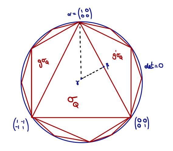
Figure 4. The decomposition of the link $L\mathcal{P}^{\mathrm{rt}}$ into Voronoï cells viewed inside the projective space $\mathbb{P}^{2}(\mathbb{R})$ of symmetric $2\times 2$ matrices. The space $|L\mathcal{A}_{2}^{\mathrm{trop}}|$ is the quotient of the closed simplex $L\sigma_{Q}$ by the action of $\Sigma_{3}$, and is the one-point compactification of the interior $|L\mathcal{A}^{\circ,\mathrm{trop}}|$ at the cusp. The space $|L\mathcal{A}_{2}^{\mathrm{trop},\mathcal{B}}|$ has an additional half-interval at every cusp.

1.4. Bordification of the moduli space of tropical abelian varieties.

In order to prove theorem 1.3, we construct an explicit bordification

$$\left|L\mathcal{A}_{g}^{\mathrm{trop},\mathcal{B}}\right|\longrightarrow\left|L\mathcal{A}_{g}^{\mathrm{trop}}\right|\ .$$

It has a boundary $\left|\partial L\mathcal{A}_{g}^{\mathrm{trop},\mathcal{B}}\right|\subset\left|L\mathcal{A}_{g}^{\mathrm{trop},\mathcal{B}}\right|$ with the property that

$$\left|L\mathcal{A}_{g}^{\mathrm{trop},\mathcal{B}}\right|\ \setminus\ \left|\partial L\mathcal{A}_{g}^{\mathrm{trop},\mathcal{B}}\right|=\left|L\mathcal{A}_{g}^{\circ,\mathrm{trop}}\right|\ .$$

The topological space $\left|L\mathcal{A}_{g}^{\mathrm{trop},\mathcal{B}}\right|$ is technically the space obtained by gluing together ‘wonderful’ compactifications [DCP95] of perfect cones $\sigma_{Q}$ by blowing up specific boundary strata which lie at infinity. It may be constructed informally as follows.

Consider the projective space $\mathbb{P}(\mathcal{Q}(V))$ whose points are projective classes of quadratic forms $\mathcal{Q}(V)$ in a vector space $V$ of dimension $g$ over $\mathbb{Q}$. The vanishing of the determinant defines a hypersurface $\mathrm{Det}\subset\mathbb{P}(\mathcal{Q}(V))$ whose complement satisfies:

$$L\mathcal{P}_{g}\ \subset\ \left(\mathbb{P}(\mathcal{Q}(V))\ \setminus\ \mathrm{Det}\right)(\mathbb{R})\ .$$

Now consider the space obtained by blowing up the subspaces $\mathbb{P}(\mathcal{Q}(V/K))$ whose points are quadratic forms with kernel $K$, for all rational subspaces $0\neq K\subset V$, in increasing order of dimension. Since $\mathbb{P}(\mathcal{Q}(V/K))$ is contained in the determinant locus $\mathrm{Det}$, every blow-up adds a new boundary component at infinity. Such a boundary component is indexed by a nested sequence $0<K_{1}<K_{2}<\ldots<K_{n}<V$, and is isomorphic to a product of projective spaces. The closure of $L\mathcal{P}_{g}$ in the iterated blow-up admits an action by $\mathrm{GL}_{g}(\mathbb{Z})$, whose quotient is the bordification $\left|L\mathcal{A}_{g}^{\mathrm{trop},\mathcal{B}}\right|$. We show in an appendix that it is homeomorphic to the Borel-Serre compactification [BS73]. Fom this construction it is not obvious that $\left|L\mathcal{A}_{g}^{\mathrm{trop},\mathcal{B}}\right|$ in fact has an algebraic structure of finite type (see §1.7) which is crucial for us.

Theorem 1.3 is proven by studying the behaviour of the differential forms (1.1) on the boundary of $\left|L\mathcal{A}_{g}^{\mathrm{trop},\mathcal{B}}\right|$. The existence of this bordification, and the techniques used to construct it, have a variety of other applications, which we discuss below.

1.5. Bordification of the tropical Torelli map.

The main thrust of this paper is to provide a general technique for constructing bordifications of spaces built out of quotients of polyhedral cells. For example, we construct a bordification

$$\left|L\mathcal{M}_{g}^{\mathrm{trop},\mathcal{B}}\right|\longrightarrow\left|L\mathcal{M}_{g}^{\mathrm{trop}}\right|$$

of the link of the moduli space of tropical curves whose existence was alluded to in [Bro21]. It is obtained by gluing together the ‘Feynman polytopes’ associated to stable graphs and provides a single geometric object whose cells are the spaces underling the Feynman motives of [BEK06, Bro17a]. This bordification is presumably equivalent to the bordification of Culler and Vogtmann’s Outer space which was constructed in [BF00, BSV18].

The bordifications of $\left|L\mathcal{A}^{\mathrm{trop}}_{g}\right|$ and $\left|L\mathcal{M}^{\mathrm{trop}}_{g}\right|$ are related as follows. The tropical Torelli map $\lambda:\left|L\mathcal{M}_{g}^{\mathrm{trop}}\right|\rightarrow\left|L\mathcal{A}_{g}^{\mathrm{trop}}\right|$ was studied in [Nag97, Bak11, CV10, MZ08, BMV11]. It is non-degenerate on the subspace $\left|L\mathcal{M}_{g}^{\mathrm{red}}\right|\subset\left|L\mathcal{M}_{g}^{\mathrm{trop}}\right|$ indexed by $3$-edge connected graphs.

Theorem 1.4.

The tropical Torelli map extends to a map $\lambda^{\mathcal{B}}$ of bordifications, giving a commutative diagram where the vertical maps are blow-downs:

$$\begin{array}[]{ccc}\left|L\mathcal{M}_{g}^{\mathrm{red},\mathcal{B}}\right|&\overset{\lambda^{\mathcal{B}}}{\longrightarrow}&\left|L\mathcal{A}_{g}^{\mathrm{trop},\mathcal{B}}\right|\\ \downarrow&&\downarrow\\ \left|L\mathcal{M}_{g}^{\mathrm{red}}\right|&\overset{\lambda}{\longrightarrow}&\left|L\mathcal{A}_{g}^{\mathrm{trop}}\right|\end{array}$$

This diagram gives relations between the cohomology of the four spaces. Note that the cohomology of $\left|L\mathcal{M}_{g}^{\mathrm{trop}}\right|$ is related to the cohomology of Kontsevich’s commutative graph complex $\mathcal{GC}_{0}$, and to the top-weight cohomology of the moduli stack $\mathcal{M}_{g}$ [CGP20]. The cohomology of the bordification $\left|L\mathcal{M}_{g}^{\mathrm{trop},\mathcal{B}}\right|$ is described by a new graph complex §8.2 which involves nested sequences of graphs related to the Hopf algebra structure on graph homology. It would be very interesting to study its homology in relation to that of $\mathcal{GC}_{0}$.

1.6. Canonical integrals of perfect cones

A further consequence of the properties of canonical forms (1.1) on the bordification of $\left|L\mathcal{A}_{g}^{\mathrm{trop}}\right|$ is that we may assign transcendental invariants by integrating over the polyhedral cones in the Voronoï decomposition.

Theorem 1.5.

Let $Q$ be a positive definite quadratic form of rank $g$, and let $\sigma_{Q}$ be the associated cone. Let $\omega\in\Omega^{d}_{\mathrm{can}}$ be any canonical form (1.1) of degree $d=\dim\sigma_{Q}$. If $\sigma_{Q}$ has rank $g$ then the following integral is finite:

(1.5) $$I_{Q}(\omega)=\int_{\sigma_{Q}}\omega<\infty\ .$$

The integrals $I_{Q}(\omega)$ satisfy quadratic relations arising from Stokes’ formula (theorem 13.13).

The condition that $\sigma_{Q}$ has rank $g$ means that $\sigma_{Q}$ meets the interior $L\mathcal{P}_{g}$ of the link of the space of positive definite matrices (i.e., it does not completely lie at infinity). In particular, every ‘perfect’ quadratic form of maximal dimension may be assigned a volume, which is non-zero. Theorem 1.5 provides interesting transcendental invariants of quadratic forms which may provide a new perspective on the extensive literature on perfect forms in relation to sphere packing problems, which was one of Voronoï’s original goals.

In the case when the cone $\sigma_{Q}$ is cographical, i.e., the image under the tropical Torelli map of the cell associated to a graph in $\left|L\mathcal{M}_{g}^{\mathrm{red}}\right|$, the integrals (1.5) reduce to the canonical integrals $I_{G}(\omega)$ studied in [Bro21]. It was proved in loc. cit. that these are generalised Feynman integrals of the sort arising in perturbative quantum field theory. An important slogan, therefore, from the present paper is that the volumes of cographical cells in the perfect cone decomposition of the space of symmetric matrices are Feynman integrals. The Borel regulator, in particular, is a linear combinations of integrals (1.5).

The arithmetic nature of the period integrals (1.5) is not known. However, a computation by Borinsky and Schnetz [BS21] implies that the volume of the principle cone for $\mathrm{GL}_{5}(\mathbb{Z})$ is a linear combination of non-trivial multiple zeta values of weight $8$ which involves $\zeta(3,5)$.

1.7. Polyhedral cell complexes

We finally turn to the main geometric constructions. Theorem 1.3 hinges upon a de Rham theorem for topological spaces obtained by gluing together quotients of polyhedra by finite group actions. In order to make sense of algebraic differential forms such as (1.1) on these spaces, we embed each polyhedron into an ambient algebraic variety, which are glued together according to the same pattern.

The most basic construction along these lines is a category, which we call $\mathrm{PLC}_{k}$, of polyhedral linear configurations over a field $k\subset\mathbb{R}$. Its objects are triples: $(\mathbb{P}(V),L_{\sigma},\sigma)$, where $V$ is a finite-dimensional vector space over $k$, $\sigma\subset\mathbb{P}(V)(\mathbb{R})$ is a closed convex polyhedron, and $L_{\sigma}\subset\mathbb{P}(V)$ is the union of linear subspaces defined by the Zariski closure of the boundary $\partial\sigma$. A morphism $\phi:(\mathbb{P}(V),L_{\sigma},\sigma)\rightarrow(\mathbb{P}(V^{\prime}),L_{\sigma^{\prime}},\sigma^{\prime})$ in this category is a linear map $\phi:\mathbb{P}(V)\rightarrow\mathbb{P}(V^{\prime})$ such that $\phi(L_{\sigma})\subset L_{\sigma^{\prime}}$ and $\phi(\sigma)\subset\sigma^{\prime}$. We demand, in addition, that $\phi:\sigma\rightarrow\sigma^{\prime}$ be either the inclusion of a face, or an isomorphism.

We then define a linear polyhedral complex to be a space assembled out of such objects (and their quotients by finite linear group actions). More precisely, it is given by a functor

$$F:\mathcal{D}\longrightarrow\mathrm{PLC}_{k}$$

where $\mathcal{D}$ is equivalent to a finite diagram category. It has a topological realisation:

$$|F|=\varinjlim_{x\in\mathcal{D}}\sigma(F(x))\ ,$$

which is the topological space obtained by gluing the polyhedra $\sigma(F(x))$ along linear maps. Examples of linear polyhedral complexes include the moduli space of tropical curves $L\mathcal{M}^{\mathrm{trop}}_{g}$ of genus $g$, where $\mathcal{D}$ is a category of stable graphs, and the moduli space of tropical abelian varieties $L\mathcal{A}^{\mathrm{trop}}_{g}$, in which case $\mathcal{D}$ is a category of cones associated to quadratic forms. The topological realisation of a polyhedral linear complex is closely related to similar notions in the literature, including stacky fans [BMV11] and generalised CW-complexes [ACP22].

However, a polyhedral linear complex has additional algebraic structure. In particular, there is a functor $\mathsf{S}F:\mathcal{D}\rightarrow\mathrm{Sch}_{k}$ to the category of schemes which picks out the first component in each triple $x\mapsto\mathbb{P}(V_{F(x)})$. We can speak of a subscheme of $F$: it is simply a subfunctor $\mathcal{X}:\mathcal{D}\rightarrow\mathrm{Sch}_{k}$ of $\mathsf{S}F$. Concretely, it is given by the data of a compatible family of subschemes $\mathcal{X}_{x}\subset\mathbb{P}(V_{F(x)})$ for every object $x$ in $\mathcal{D}$. A global algebraic differential form on a polyhedral linear complex $F$ with poles along $\mathcal{X}$ is simply an element of

(1.6) $$\Omega^{\bullet}(F\backslash\mathcal{X})=\varprojlim_{x\in\mathcal{D}}\,\Omega^{\bullet}\left(\mathbb{P}(V_{F(x)})\backslash\mathcal{X}_{x}\right)\ .$$

It is a compatible system of differential forms on $\mathbb{P}(V_{F(x)})$ with poles along $\mathcal{X}_{x}$ for each $x$. Our main examples are: the subscheme of $L\mathcal{M}_{g}^{\mathrm{trop}}$ defined by the graph hypersurface locus, and the subscheme of $L\mathcal{A}_{g}^{\mathrm{trop}}$ defined by the determinant locus $\mathrm{Det}$.

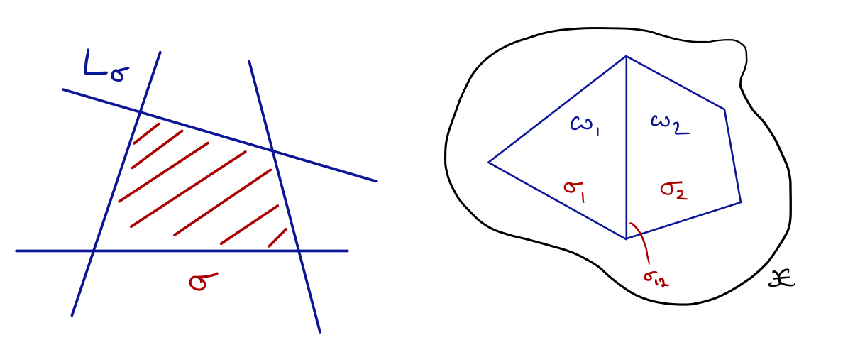
Figure 5. Left: a polyhedral linear configuration in $\mathbb{P}^{2}$. Right: two polyhedra $\sigma_{1}$, $\sigma_{2}$ are glued together along the common face $\sigma_{12}=\sigma_{1}\cap\sigma_{2}$. An algebraic differential form $\omega$ defines two forms $\omega_{i}=\omega\big{|}_{\sigma_{i}}$, for $i=1,2$, which coincide on $\sigma_{12}$. The form $\omega$ has poles along a subscheme $\mathcal{X}$, which, as depicted, may not necessarily meet the topological realisation $\sigma_{1}\cup_{\sigma_{12}}\sigma_{2}$.

The above definitions can be generalised. The most important construction, for our purposes, is a category $\mathrm{BLC}_{k}$ whose objects consist of iterated blow-ups of polyhedral linear configurations along linear subspaces. They are ‘wonderful’ compactifications of linear polyhedra in the sense of [DCP95]. Using this concept, we can efficiently define the bordifications mentioned earlier. For instance, we construct a functor

$$L\mathcal{A}_{g}^{\mathrm{trop},\mathcal{B}}:\mathcal{D}_{g}^{\mathrm{perf},\mathcal{B}}\longrightarrow\mathrm{BLC}_{\mathbb{Q}}$$

from a suitable diagram category to $\mathrm{BLC}_{\mathbb{Q}}$. It is defined by blowing up the subspaces of quadratic forms with a non-trivial rational kernel which meet each cone in the Voronoï decomposition. A key point is that that this space is a diagram of finitely many algebraic varieties with extra structure; the informal definition of $\left|L\mathcal{A}_{g}^{\mathrm{trop},\mathcal{B}}\right|$ given earlier in this introduction a priori involved infinitely many blow-ups.

The next theorem is the key geometric input in the proof of theorems 1.1 and 1.3.

Theorem 1.6.

There is a commutative diagram

$$\begin{array}[]{ccc}\partial L\mathcal{A}_{g}^{\mathrm{trop},\mathcal{B}}&\hookrightarrow&L\mathcal{A}_{g}^{\mathrm{trop},\mathcal{B}}\\ \downarrow_{\pi^{\mathcal{B}}}&&\downarrow_{\pi^{\mathcal{B}}}\\ \partial L\mathcal{A}_{g}^{\mathrm{trop}}&\hookrightarrow&L\mathcal{A}_{g}^{\mathrm{trop}}\end{array}$$

where the vertical maps $\pi^{\mathcal{B}}$ are canonical blow-downs. The strict transform of the determinant subscheme $\mathrm{Det}\subset L\mathcal{A}_{g}^{\mathrm{trop}}$ defines a subscheme

$$\widetilde{\mathrm{Det}}\subset L\mathcal{A}_{g}^{\mathrm{trop},\mathcal{B}}$$

which satisfies $\pi^{\mathcal{B}}:\widetilde{\mathrm{Det}}\rightarrow\mathrm{Det}$, and has the property

(1.7) $$\widetilde{\mathrm{Det}}\cap\left|L\mathcal{A}_{g}^{\mathrm{trop},\mathcal{B}}\right|=\emptyset\ .$$

On topological realisations, one has a commutative diagram of topological spaces

$$\begin{array}[]{ccc}&&\left|L\mathcal{A}_{g}^{\mathrm{trop},\mathcal{B}}\right|\,\setminus\,\left|\partial L\mathcal{A}_{g}^{\mathrm{trop},\mathcal{B}}\right|\\ &\nearrow&\downarrow\\ \left|L\mathcal{A}_{g}^{\circ,\mathrm{trop}}\right|&\rightarrow&\left|L\mathcal{A}_{g}^{\mathrm{trop}}\right|\,\setminus\,\left|\partial L\mathcal{A}_{g}^{\mathrm{trop}}\right|\end{array}$$

where all arrows are isomorphisms. The open locus $\left|L\mathcal{A}_{g}^{\circ,\mathrm{trop}}\right|$ is homeomorphic to the locally symmetric space $L\mathcal{P}_{g}/\mathrm{GL}_{g}(\mathbb{Z})=\mathbb{R}_{>0}^{\times}\setminus\mathcal{P}_{g}/\mathrm{GL}_{g}(\mathbb{Z})$.

A similar theorem holds for the moduli space $L\mathcal{M}_{g}^{\mathrm{trop}}$ of tropical curves (§8).

1.8. ‘Motives’ of quadratic forms

Hereafter, a motive refers to an object in a suitable Tannakian $\mathcal{H}_{\mathbb{Q}}$ category of realisations, following Deligne [Del89]. An object $M$ in $\mathcal{H}_{\mathbb{Q}}$ has Betti and de Rham realisations $M_{B}$, $M_{dR}$ and a period pairing $M_{B}^{\vee}\otimes_{\mathbb{Q}}M_{dR}\rightarrow\mathbb{C}$. The property (1.7) of the determinant locus enables us to define a canonical object $\mathrm{mot}_{Q}$ associated to a positive definite quadratic form $Q$ such that the integral (1.5) is a period (definition 15.1). In the special case when $\sigma_{Q_{G}}=\sigma_{G}$ is a cographical cone in the image of the tropical Torelli map, $\mathrm{mot}_{Q_{G}}$ is equivalent to the graph motive defined in [BEK06]. This construction provides, in particular, a motivic interpetation of the Borel regulator.

1.9. ‘Motives’ associated to $\mathrm{GL}_{g}(\mathbb{Z})$.

Similarly, we may find a motivic interpretation of the canonical cohomology of $\mathrm{GL}_{g}(\mathbb{Z})$. For every $g>1$ and $d\geq 0$ we define a cohomology group $H^{d}_{c}(g)$ consisting of closed compatible families of algebraic differential forms with poles along the determinant locus (1.6), modulo exact forms. There is a natural map:

$$H^{d}_{c}(g)\longrightarrow H_{c}^{d}(L\mathcal{P}_{g}/\mathrm{GL}_{g}(\mathbb{Z});\mathbb{R})$$

which is injective on $\Omega^{d}_{c}(g)\subset H^{d}_{c}(g)$: in particular, $H^{d}_{c}(g)$ contains all the compactly-supported cohomology classes for $\mathrm{GL}_{g}(\mathbb{Z})$ which are described in theorem 1.1. Integration of differential forms defines a pairing

$$H^{\mathrm{lf}}_{d}(\mathrm{GL}_{g}(\mathbb{Z});\mathbb{Q})\otimes_{\mathbb{Q}}H^{d}_{c}(g)\longrightarrow\mathbb{C}$$

where $H^{\mathrm{lf}}$ denotes locally finite (Borel-Moore) homology.

Theorem 1.7.

There is an object $\mathsf{M}^{d}_{g}$ of $\mathcal{H}_{\mathbb{Q}}$ equipped with a pair of canonical linear maps

$$H^{\mathrm{lf}}_{d}(\mathrm{GL}_{g}(\mathbb{Z});\mathbb{Q}) \longrightarrow (\mathsf{M}^{d}_{g})_{B}^{\vee}$$

$$H^{d}_{c}(g) \longrightarrow (\mathsf{M}^{d}_{g})_{dR}$$

such that the integration pairing factors through the period pairing: $(\mathsf{M}^{d}_{g})_{B}^{\vee}\otimes_{\mathbb{Q}}(\mathsf{M}^{d}_{g})_{dR}\rightarrow\mathbb{C}$.

This theorem implies that the part of the locally finite homology $H^{\mathrm{lf}}_{d}(\mathrm{GL}_{g}(\mathbb{Z});\mathbb{Q})$ which pairs non-trivially with $H^{d}_{c}(g)$ is motivic, since $\mathsf{M}^{d}_{g}$ lies in the Tannakian subcategory of $\mathcal{H}_{\mathbb{Q}}$ generated by the cohomology of algebraic varieties over $\mathbb{Q}$. In particular, the theorem provides a motivic interpretation of the integrals of canonical differential forms over homology cycles, including the volume integrals over fundamental domains considered by Minkowski. The objects $\mathsf{M}$ are interesting: for example, $\mathsf{M}^{5}_{3}$ is a non-trivial extension of $\mathbb{Q}(-3)$ by $\mathbb{Q}(0)$ with period $6\,\zeta(3)$, which is the volume of a fundamental domain for $\mathrm{GL}_{3}(\mathbb{Z})$ with respect to the form $\omega^{5}$ (1.1).

One can define other motives associated to spaces such as $L\mathcal{P}_{g}/\mathrm{GL}_{g}(\mathbb{Z})$, for example, by allowing differential forms with poles along other loci. For example, using a theorem of Sullivan one may define a weight zero Tate motive which captures the entire cohomology of $\mathrm{GL}_{g}(\mathbb{Z})$. Its periods are only rational numbers, however.

1.10. Plan and further comments

Section §2 introduces a general notion of polyhedral cell complexes in algebraic varieties, for which we prove a cellular homology and de Rham cohomology theorem in §3. In section §4 we study the particular subcategory of linear polyhedral cell complexes $\mathrm{PLC}_{k}$, and their iterated blow-ups in §5.

The first application of this theory is to the moduli space of tropical curves §6, and its bordification §7-8. The discussion of the moduli space of tropical abelian varieties begins in §9 with a study of polyhedra in spaces of quadratic forms and their blow-ups. In section 10 we study $L\mathcal{A}_{g}^{\mathrm{trop}}$ and define its perfect cone bordification $L\mathcal{A}_{g}^{\mathrm{trop},\mathcal{B}}$. Section 11 studies the properties of the determinant locus and its strict transform. In section 12, we construct the bordification of the tropical Torelli map.

From section 13 onwards, we study the properties of canonical forms and their integrals, and in §14 we prove the main results on the cohomology of $\mathrm{SL}_{g}(\mathbb{Z})$ and $\mathrm{GL}_{g}(\mathbb{Z})$ mentioned in this introduction. Finally, §15 discusses the periods and motives associated to canonical integrals and in an appendix we discuss the relation between the Borel-Serre compactification and the space $\left|L\mathcal{A}^{\mathrm{trop},\mathcal{B}}_{g}\right|$ defined algebraically using blow-ups. We expect that the methods of this paper may be used to define and study the geometric spaces, differential forms, and cohomology classes associated to other types of graph complexes (see, e.g., [BM19]), as well as the quotients of symmetric spaces by general linear groups over number fields.

1.11. Acknowledgements

This project has received funding from the European Research Council (ERC) under the European Union’s Horizon 2020 research and innovation programme (grant agreement no. 724638). The author thanks Trinity College, Dublin for a Simons visiting Professorship during which much of this work was carried out and the University of Geneva, where it was completed. Very many thanks are owed to Chan, Galatius, Grushevsky and Payne for extensive discussions on $\mathcal{A}_{g}$ which motivated this work. The author benefited from discussions with Berghoff, Dupont, Grobner and Vogtmann, whose online notes on the Borel-Serre construction were most useful. The author is especially grateful to Melody Chan for feedback and corrections.

2. Algebraic polyhedral cell complexes

We describe a formalism to construct algebraic models of certain topological spaces defined by gluing together polyhedral cells according to a diagram category. In the first instance, the cells will be objects of a very general category $\mathcal{PC}_{k}$, but for the applications we shall work with more restrictive subcategories $\mathrm{PLC}_{k}$ of convex linear polyhedra in projective space, and $\mathrm{BLC}_{k}$ of their blow-ups along linear spaces.

2.1. A category of polyhedral cells

Let $k\subset\mathbb{C}$ be a field. There are many situations in which one has a polyhedron embedded in the real or complex points of an algebraic variety. Since convexity does not make sense in this generality, one must define a polyhedron in an algebraic variety using different concepts. To this end, let us denote by $\mathcal{PC}_{k}$ the category whose objects are triples $(P,L,\sigma)$ defined recursively as follows:

• $P$ is a smooth scheme over $k$.

• $\sigma\subset P(\mathbb{C})$ is homeomorphic to a closed ball $B_{n}$ of dimension $n\geq 0$, i.e., there is a continuous map $g:B_{n}\hookrightarrow P(\mathbb{C})$ such that $g:B_{n}\cong\sigma$. We call $n$ the dimension of $(P,L,\sigma)$. It may be strictly smaller than the dimension of $P$.

• The boundary of $\sigma$ satisfies $\partial\sigma=\sigma\cap L(\mathbb{C})$, where $L\subset P$ is a subscheme with finitely many distinct smooth irreducible components $L_{i}$, $i\in I$.

• Let $n\geq 1$. For every $i\in I$ such that $L_{i}(\mathbb{C})\cap\sigma$ is non-empty, the triple

  (2.1) $$\left(L_{i},\bigcup_{L_{j}\neq L_{i}}L_{i}\cap L_{j},\sigma\cap L_{i}(\mathbb{C})\right)$$

  is required to be an object in $\mathcal{PC}_{k}$ of dimension $<n$.

The objects in $\mathcal{PC}_{k}$ of dimension $0$ are triples $(P,L,\sigma)$ where $\sigma\subset L(\mathbb{C})$ is a point. For any object $(P,L,\sigma)$, one has $\partial\sigma=\bigcup_{i\in I}\sigma_{i}$, where $\sigma_{i}=\sigma\cap L_{i}(\mathbb{C})$ is of smaller dimension. Therefore by repeatedly taking boundaries, one obtains a stratification on $\sigma$ giving a structure of a regular CW-complex on the closed ball $B_{n}$. Note that the fourth condition $\partial\sigma=\sigma\cap L(\mathbb{C})$ captures a notion of convexity (it fails for non-convex Euclidean polyhedra). A morphism:

$$\phi:(P,L,\sigma)\rightarrow(P^{\prime},L^{\prime},\sigma^{\prime})$$

is given by a morphism $\phi:P\rightarrow P^{\prime}$ such that $\phi(L)\subset L^{\prime}$ and $\phi(\sigma)\subset\sigma^{\prime}$. For any subset $J\subset I$, let $L_{J}=\bigcap_{j\in J}L_{j}$. A face map is an inclusion of a face

(2.2) $$\iota_{J}:\left(L_{J},\bigcup_{j\in I\setminus J}L_{J\cup\{j\}},\sigma\cap L_{J}(\mathbb{C})\right)\longrightarrow(P,L,\sigma)$$

where $\sigma\cap L_{J}(\mathbb{C})\neq\emptyset$. A facet of $(P,L,\sigma)$ is a face (2.1) of dimension $\dim\sigma-1$.

Example 2.1.

Let $P=\mathbb{P}^{n}_{\mathbb{Q}}$ denote projective space of dimension $n$ with homogeneous coordinates $(x_{0}:\ldots:x_{n})$. The algebraic simplex is the triple $(\mathbb{P}^{n}_{\mathbb{Q}},L,\sigma)$, where $L=V(x_{0}\ldots x_{n})$ is the union of coordinate hyperplanes, and $\sigma\subset\mathbb{P}^{n}_{\mathbb{Q}}(\mathbb{R})$ is defined by the standard coordinate simplex region $x_{i}\geq 0$. Its faces are algebraic simplices of smaller dimension.

Notation 2.2.

Define the product $\prod_{i=1}^{n}(P_{i},L_{i},\sigma_{i})$ of objects $(P_{i},L_{i},\sigma_{i})$ in $\mathcal{PC}_{k}$ by

$$\left(P_{1}\times\ldots\times P_{n}\ ,\ \bigcup_{i=1}^{n}P_{1}\times\ldots\times P_{i-1}\times L_{i}\times P_{i+1}\times\ldots\times P_{n}\ ,\ \sigma_{1}\times\ldots\times\sigma_{n}\right)\ .$$

Given morphisms $f_{1},\ldots,f_{n}$ in $\mathcal{PC}_{k}$, denote by $f_{1}\times\ldots\times f_{n}$ the induced morphism on products. There are canonical projection morphisms for any ordered finite sets $I\supset J$:

(2.3) $$p_{I/J}\ :\ \prod_{i\in I}(P_{i},L_{i},\sigma_{i})\rightarrow\prod_{j\in J}(P_{j},L_{j},\sigma_{j})$$

There are two natural functors, both of which preserve products:

(2.4) $$\begin{array}[]{ccccccc}\sigma:\mathcal{PC}_{k}&\longrightarrow&\mathcal{T}op&\qquad\hbox{ and }&\mathsf{S}:\mathcal{PC}&\longrightarrow&\mathrm{Sch}_{k}\\ \sigma(P,L,\sigma)&=&\sigma&&\mathsf{S}(P,L,\sigma)&=&P\end{array}$$

2.2. Algebraic polyhedral cell complexes

Let $\mathcal{C}_{k}$ denote a subcategory of $\mathcal{PC}_{k}$. The main cases of interest are $\mathcal{C}_{k}=\mathrm{PLC}_{k}$ (§4) and $\mathcal{C}_{k}=\mathrm{BLC}_{k}$ (§5).

Definition 2.3.

A $\mathcal{C}_{k}$-complex is a functor

(2.5) $$F:\mathcal{D}\longrightarrow\mathcal{C}_{k}$$

where $\mathcal{D}$ is equivalent to a finite category.

A morphism $(\Phi,\phi)$ between two functors $F:\mathcal{D}\rightarrow\mathcal{C}_{k}$ and $F^{\prime}:\mathcal{D^{\prime}}\rightarrow\mathcal{C}_{k}$ is the data of:

(i) a functor $\phi:\mathcal{D}\rightarrow\mathcal{D^{\prime}}$ and

(ii) a natural transformation $\Phi:F\rightarrow F^{\prime}\circ\phi$.

To spell this out, $\Phi$ is the data, for every object $x$ of $\mathcal{D}$, of a morphism

$$\Phi_{x}:F(x)\longrightarrow(F^{\prime}\circ\phi)(x)\qquad\hbox{ in }\mathcal{PC}_{k}$$

such that, for every morphism $f:x\rightarrow y$ in $\mathcal{D}$, there is a commutative diagram

$$F(x)\quad \overset{\Phi_{x}}{\longrightarrow} (F^{\prime}\circ\phi)(x)\qquad$$

$$\downarrow_{F(f)} \quad\,\,\,\downarrow_{(F^{\prime}\circ\phi)(f)}$$

$$F(y)\quad \overset{\Phi_{y}}{\longrightarrow} (F^{\prime}\circ\phi)(y)\qquad\ .$$

In particular, any functor $\phi:\mathcal{D}\rightarrow\mathcal{D}^{\prime}$ induces a morphism $(\phi,\mathrm{id})$ between $F=F^{\prime}\circ\phi$ and $F^{\prime}$. If $\phi$ is an equivalence, then $F$ and $F^{\prime}$ are isomorphic. In particular, by replacing $\mathcal{D}$ with an equivalent category, we may assume that $\mathcal{D}$ is itself finite.

Definition 2.4.

The topological realisation of (2.5) is the topological space

(2.6) $$|F|=\varinjlim_{x\in\mathrm{Ob}(\mathcal{D})}\sigma(F(x))\ .$$

By taking limits, a morphism $(\Phi,\phi)$ from $F$ to $F^{\prime}$ induces a continuous map between their topological realisations. We denote it by $|\Phi|:|F|\longrightarrow|F^{\prime}|.$

2.3. Subschemes

Let $F:\mathcal{D}\rightarrow\mathcal{PC}_{k}$ be a functor (2.5) as above.

Definition 2.5.

Define a closed (resp. open) subscheme of $F$ to be a functor

$$\mathcal{X}:\mathcal{D}\longrightarrow\mathrm{Sch}_{k}$$

such that $\mathcal{X}_{x}$ is a closed (resp. open) subscheme of $\mathsf{S}F_{x}$, for all objects $x$ of $\mathcal{D}$, and such that the canonical embedding $i_{x}:\mathcal{X}_{x}\subset\mathsf{S}F_{x}$ is a natural transformation $i:\mathcal{X}\rightarrow\mathsf{S}F$. If $K=\mathbb{R}$ or $\mathbb{C}$, and contains $k\subset K$, then the set of $K$-points defines a topological space

$$|\mathcal{X}(K)|=\varinjlim_{x\in\mathcal{D}}\mathcal{X}_{x}(K)$$

with the analytic topology.

Definition 2.5 is analogous to that of a subfunctor. It means that for all morphisms $f:x\rightarrow y$ in $\mathcal{D}$ there is a commutative diagram

$$\begin{array}[]{ccc}\mathsf{S}F_{x}&\overset{F(f)}{\longrightarrow}&\mathsf{S}F_{y}\\ \rotatebox[origin={c}]{90.0}{$\subseteq$}&&\rotatebox[origin={c}]{90.0}{$\subseteq$}\\ \mathcal{X}_{x}&\overset{X(f)}{\longrightarrow}&\mathcal{X}_{y}\end{array}$$

and hence the morphisms between $\mathcal{X}_{x}$ are obtained by restricting those from $\mathsf{S}F$.

Definition 2.6.

We say that a closed subscheme $\mathcal{Z}$ of $\mathsf{S}F$ is at infinity, which we denote by $|F|\cap\mathcal{Z}=\emptyset$, if its image does not meet any of the polyhedra $\sigma(F_{x})$:

$$\sigma(F_{x})\cap i_{x}(\mathcal{Z}_{x})(\mathbb{C})=\emptyset\ \hbox{ for all }\ x\in\mathrm{Ob}(\mathcal{D}).$$

Similarly, for an open subscheme $U$ of $F$ we write $|F|\subset U$ if

$$\sigma(F_{x})\ \subset\ U_{x}(\mathbb{C})\ \hbox{ for all }\ x\in\mathrm{Ob}(\mathcal{D}).$$

Definition 2.7.

Given an open subscheme $\mathcal{U}$ of $\mathsf{S}F$ such that $|F|\subset\mathcal{U}$, define

(2.7) $$F\cap\mathcal{U}:\mathcal{D} \longrightarrow \mathcal{PC}_{k}$$

$$x \mapsto (F\cap\mathcal{U})_{x}=(\mathcal{U}_{x},L_{x}\cap U,\sigma)\ ,$$

which we may view as an (open) subfunctor of $F:\mathcal{D}\rightarrow\mathcal{PC}_{k}$.

2.4. Algebraic and meromorphic differential forms

Definition 2.8.

Consider a $\mathcal{C}_{k}$-complex $F:\mathcal{D}\rightarrow\mathcal{C}_{k}$ and a subscheme $\mathcal{X}\subset\mathsf{S}F$. A global differential form of degree $d$ on $F$ with poles along $\mathcal{X}$ is an element of the limit

$$\Omega^{d}(\mathsf{S}F\backslash\mathcal{X})=\varprojlim_{x\in\mathrm{Ob}(\mathcal{D})}\Omega^{d}(\mathsf{S}F(x)\backslash\mathcal{X}(x))\ .$$

Equivalently, it is a collection, for every $x\in\mathrm{Ob}(\mathcal{D})$, of regular forms $\omega_{x}\in\Omega^{d}(\mathsf{S}F(x)\backslash\mathcal{X}(x))$ which are compatible in the sense that

(2.8) $$F(f)^{*}(\omega_{x})=\omega_{y}\quad\hbox{ for every }\quad f\in\mathrm{Hom}_{\mathcal{D}}(x,y)\ .$$

The graded vector space $\Omega^{\bullet}(\mathsf{S}F\backslash\mathcal{X})=\bigoplus_{d}\Omega^{d}(\mathsf{S}F\backslash\mathcal{X})$ is a differential graded algebra. We may also write it $\Omega^{\bullet}(F\backslash\mathcal{X})$, bearing in mind that it depends only on the functor $\mathsf{S}F$.

Consider an object $(P,L,\sigma)$ of $\mathcal{PC}_{k}$. Let us denote by

$$\Omega_{\mathrm{mer}}^{d}\left((P,L,\sigma)\right)=\varinjlim_{U:\sigma\subset U(\mathbb{C})}\Omega^{d}(U;k)$$

the space of meromorphic differential forms which are regular on an open affine subset $U$ of $P$ whose complex points contain $\sigma$. Such a form may be restricted to the faces of $\sigma$, and so $\Omega_{\mathrm{mer}}^{\bullet}=\bigoplus_{d\geq 0}\Omega_{\mathrm{mer}}^{d}$ is a contravariant functor from $\mathcal{PC}_{k}$ to the category of DGA’s.

Definition 2.9.

Consider a $\mathcal{C}_{k}$-complex $F:\mathcal{D}\rightarrow\mathcal{C}_{k}$. A meromorphic differential form of degree $d$ on $F$ is an element of the projective limit

$$\Omega_{\mathrm{mer}}^{d}(F)=\varprojlim_{x\in\mathrm{Ob}(\mathcal{D})}\Omega_{\mathrm{mer}}^{d}(F(x))\ .$$

It is a compatible collection of meromorphic forms $\omega_{x}\in\Omega^{d}_{\mathrm{mer}}(F(x))$ for $x\in\mathrm{Ob}(\mathcal{D})$. The total space $\Omega_{\mathrm{mer}}^{\bullet}(F)=\bigoplus_{d\geq 0}\Omega_{\mathrm{mer}}^{d}(F)$ is a differential graded algebra.

Examples 2.10.

The DGA of meromorphic forms $\Omega_{\mathrm{mer}}^{d}\left(\mathbb{P}^{n}_{\mathbb{Q}},L,\sigma\right)$ on an algebraic simplex (Example 2.1) contains the polynomial forms on $\sigma$ in the sense of Sullivan [Sul77].

Definition 2.11.

The $\mathbb{C}$-differential graded algebra of smooth forms on $|F|$ is defined to be

(2.9) $$\mathcal{A}^{\bullet}(|F|)=\varprojlim_{x\in\mathrm{Ob}(\mathcal{D})}\mathcal{A}^{\bullet}(\sigma(F_{x}))\ ,$$

where $\mathcal{A}^{\bullet}(\sigma(F_{x}))$ denotes the algebra of smooth differential forms over $\mathbb{C}$ which are defined in an open neighbourhood of $\sigma(F_{x})$ inside $\mathsf{S}F_{x}(\mathbb{C})$. When $k\subset\mathbb{R}$, and all polyhedra $\sigma(F_{x})$ are in fact contained in $\mathsf{S}F_{x}(\mathbb{R})$ (which will always be the case in our applications) then $\mathcal{A}^{\bullet}(|F|)$ has a real structure $\mathcal{A}^{\bullet}(|F|;\mathbb{R})$ consisting of the $\mathbb{R}$-subalgebra of real forms.

If $\mathcal{X}$ is at infinity $\mathcal{X}\cap|F|=\emptyset$, then there are natural maps of DGA’s:

(2.10) $$\Omega^{\bullet}(\mathsf{S}F\backslash\mathcal{X})\ \subset\ \Omega_{\mathrm{mer}}^{\bullet}(F)\longrightarrow\mathcal{A}^{\bullet}(|F|)\ .$$

Definition 2.12.

Define smooth (resp. global algebraic) cohomology groups:

(2.11) $$H^{n}_{dR}(|F|;\mathbb{C})=H^{n}(\mathcal{A}^{\bullet}(|F|))\quad(\hbox{resp. }\quad H^{n}_{dR}(\mathsf{S}F\backslash\mathcal{X})=H_{dR}^{n}(\Omega^{\bullet}(F\backslash\mathcal{X})))\ .$$

The former is a vector space over $\mathbb{C}$; the latter a vector space over $k$.

If $\mathcal{X}\cap|F|=\emptyset$, there is a natural map $H^{n}_{dR}(\mathsf{S}F\backslash\mathcal{X})\rightarrow H^{n}_{dR}(|F|)$.

3. Homology and cohomology of polyhedral complexes

3.1. Assumptions.

Let $\mathcal{C}_{k}$ be a subcategory of $\mathcal{PC}_{k}$ such that:

1. Every face of every object $(P,L,\sigma)$ in $\mathcal{C}_{k}$ is also an object of $\mathcal{C}_{k}$, and the corresponding face map is a morphism in $\mathcal{C}_{k}$.

2. All morphisms $f:(P,L,\sigma)\rightarrow(P^{\prime},L^{\prime},\sigma^{\prime})$ in $\mathcal{C}_{k}$ are either face maps, or induce homeomorphisms on topological realisations $f:\sigma\cong\sigma^{\prime}.$

In particular, the topological realisation $f:\sigma\rightarrow\sigma^{\prime}$ of any morphism in $\mathcal{C}_{k}$ is necessarily injective. For every $(P,L,\sigma)$ of dimension $n\geq 1$ one has

(3.1) $$H_{r}(\sigma,\partial\sigma;\mathbb{Z})=\begin{cases}\mathbb{Z}\quad\hbox{ if }r=n\\ 0\quad\hbox{ otherwise }\end{cases}\ .$$

An orientation on $\sigma$ is a generator $\omega\in H_{n}(\sigma,\partial\sigma;\mathbb{Z})$ if $n\geq 1$ or $\omega\in H_{0}(\sigma)$ if $n=0$. The two main categories of interest, $\mathrm{PLC}_{k}$ and $\mathrm{BLC}_{k}$, satisfy $(1)$ and $(2)$. An important remark is that an isomorphism between objects of $\mathcal{C}_{k}$ induces isomorphisms of their faces.

3.2. Cellular homology of a polyhedral $\mathcal{C}_{k}$-complex

Let $\mathcal{C}_{k}$ be a category satisfying the assumptions above and let $F:\mathcal{D}\rightarrow\mathcal{C}_{k}$ be a $\mathcal{C}_{k}$-complex.

Definition 3.1.

Define the face complex $\left(\mathfrak{C}_{F}\right)_{n}$ of $F$ to be the graded $\mathbb{Q}$-vector space with generators $[\sigma,\omega]$, where $\sigma$ is any face of dimension $n$ of the topological realisation $\sigma F_{x}$ of an object $x$ of $\mathcal{D}$, and $\omega$ is an orientation on $\sigma$. These symbols are subject to relations:

$$(i) \qquad[\sigma,\lambda\omega]=\lambda[\sigma,\omega]\qquad\hbox{ for any }\lambda\in\mathbb{Z}\ ,$$

$$(ii) \qquad\,\,\,\,[\sigma,\omega]=[\sigma^{\prime},\omega^{\prime}]$$

whenever $\sigma$, $\sigma^{\prime}$ are $n$-dimensional faces of $\sigma(F_{x})$, $\sigma(F_{y})$ respectively, and $g:x\rightarrow y$ is a morphism in $\mathcal{D}$ which restricts to an isomorphism $\sigma F(g):\sigma\overset{\sim}{\rightarrow}\sigma^{\prime}$ which sends $\omega$ to $\omega^{\prime}$.

Define a differential $d:\left(\mathfrak{C}_{F}\right)_{n}\rightarrow\left(\mathfrak{C}_{F}\right)_{n-1}$ by

(3.2) $$d[\sigma,\omega]=\sum_{\tau}\,[\tau,\omega\big{|}_{\tau}]$$

where the sum is over all facets $\tau$ of $\sigma$, where $\dim\tau=\dim\sigma-1$, and $\omega\big{|}_{\tau}$ is the image of $\omega$ under the boundary map $H_{n}(\sigma,\partial\sigma)\rightarrow H_{n-1}(\tau,\partial\tau)$. One checks that $d^{2}=0$.

Theorem 3.2.

There is a natural isomorphism $H_{n}(\mathfrak{C}_{F})\overset{\sim}{\longrightarrow}H_{n}(|F|;\mathbb{Q})$.

3.3. Differential forms and de Rham complex

The following results are valid for any complex of differential forms $\mathcal{A}^{n}$ which computes the cohomology of $\sigma$ and its boundary:

(3.3) $$H^{\bullet}(\mathcal{A}^{n}(\sigma))\cong H^{n}(\sigma;\mathbb{C})\quad\hbox{ and }\quad H^{\bullet}(\mathcal{A}^{n}(\partial\sigma))=H^{n}(\partial\sigma;\mathbb{C})$$

and which furthermore are extendable in the sense of [Sul77, §7]:

(3.4) $$i^{*}:\mathcal{A}^{\bullet}(\sigma)\longrightarrow\mathcal{A}^{\bullet}(\partial\sigma)\quad\hbox{ is surjective, }$$

where $i:\partial\sigma\subset\sigma$ denotes the inclusion map. As suggested by the notation, these two properties hold for the complex of smooth differential forms.

Theorem 3.3.

Let $\mathcal{A}^{n}$ satisfy (3.3) and (3.4) as above. Let $F:\mathcal{D}\rightarrow\mathcal{C}_{k}$ be a $\mathcal{C}_{k}$-complex, and define the de Rham complex of $F$ via (2.9). There is an isomorphism

$$H^{n}\left(\mathcal{A}^{\bullet}(\left|F\right|)\right)\overset{\sim}{\longrightarrow}H^{n}\left(|F|;\mathbb{C}\right)\ ,$$

where $H^{n}\left(|F|;\mathbb{C}\right)=H_{n}(|F|;\mathbb{C})^{\vee}$, which is induced by a bilinear pairing

(3.5) $$H^{n}\left(\mathcal{A}^{\bullet}(|F|)\right)\otimes H_{n}(|F|) \longrightarrow \mathbb{C}$$

$$\omega\otimes\gamma \mapsto \int_{\gamma}\omega\ .$$

By theorem 3.2, it may be interpreted as a pairing $H^{n}\left(\mathcal{A}^{\bullet}(|F|)\right)\otimes H_{n}(\mathfrak{C}(F))\rightarrow\mathbb{C}.$

Before proceeding with the proof, note that the integral (3.5) makes sense because a differential form $\omega\in\mathcal{A}^{\bullet}(F)$ gives rise to a well-defined smooth differential form on each simplex of $|F|$, because of the compatibility condition (2.8). The integral converges because the simplices in $|F|$ are compact, and have finitely many isomorphism classes.

Remark 3.4.

Sullivan defined a differential graded algebra of polynomial differential forms for simplicial complexes [Sul77, §7, (i), p. 297], and proved that it satisfies the extendability condition (3.4). Since they are special cases of meromorphic forms, his argument implies that the induced map $H^{n}(\Omega^{\bullet}_{\mathrm{mer}}(F))\rightarrow H^{n}(\mathcal{A}^{\bullet}(F))$ is surjective.

Even though the complex $\Omega_{\mathrm{mer}}^{\bullet}(F)$, and hence its cohomology, has a $k$-structure, the map $H^{n}(\Omega^{\bullet}_{\mathrm{mer}}(F))\rightarrow H^{n}(\mathcal{A}^{\bullet}(|F|))$ is not an isomorphism and so cannot be used to define a rational structure on the de Rham cohomology $H^{n}\left(\mathcal{A}^{\bullet}(|F|)\right)$. Put another way, the periods one obtains by integration (3.5) depends on the location of the poles of $\omega$.

3.4. Proof of theorems 3.2 and 3.3

The proof of theorem 3.2 is standard (compare with [Hat02, Theorem 2.35], [MBW22]). Consider the filtration of $X=|F|$ by subspaces

$$X_{p}=\mathrm{Im}\left(\coprod_{\dim\sigma_{x}=p}\sigma_{x}\longrightarrow X\right)$$

where the disjoint union is over all faces of polyhedral cells dimension $p$. It induces a filtration $F_{p}C_{\bullet}(X)=C_{\bullet}(X_{p})$ on the singular chain complex, giving rise to a spectral sequence

$$E^{1}_{p,q}=H_{p+q}(\mathrm{gr}^{F}_{p}C_{\bullet}(X))\cong H_{p+q}(X_{p},X_{p-1})$$

which converges to $\mathrm{gr}^{F}_{\bullet}H_{p+q}(X)$. The complex $(E^{1}_{p,q},d^{1})$ takes the form:

(3.6) $$\cdots\longrightarrow H_{p+q}(X_{p},X_{p-1})\longrightarrow H_{p+q-1}(X_{p-1},X_{p-2})\longrightarrow\cdots$$

where the maps are induced on the level of chains by the boundary map. By definition of $X_{p}$ there is a natural morphism

(3.7) $$\bigoplus_{\dim\sigma_{x}=p}\left(H_{p}(\sigma_{x},\partial\sigma_{x})\right)/\mathrm{Aut}_{\mathcal{D}}(\sigma_{x})\longrightarrow H_{p}(X_{p},X_{p-1})$$

where the sum is over all equivalence classes of faces, where two faces $\sigma_{x},\sigma_{y}$ are equivalent if they have the same image in $X$, and $\mathrm{Aut}_{\mathcal{D}}(\sigma_{x})$ is the subgroup of automorphisms on the face $\sigma_{x}$ induced by morphisms in the category $\mathcal{D}$. The map (3.7) is surjective since the intersections $\sigma_{x}\cap\sigma_{y}$ between all non-isomorphic faces $\sigma_{x},\sigma_{y}$ are unions of faces of dimension $\leq p-1$, and contained in $X_{p-1}$. Since $H_{p+q}(\sigma_{x},\partial\sigma_{x})$ is concentrated in degree $q=0$ (3.1) this proves that the spectral sequence degenerates at $E^{1}$, and the cohomology of $X$ is isomorphic to the cohomology of the complex (3.6) on setting $q=0$. In order to identify this complex with the face complex, one may observe that $H_{p+q}(\sigma_{x},\partial\sigma_{x})\cong H^{\mathrm{lf}}_{p+q}(\overset{\circ}{\sigma}_{x})$ is isomorphic to the locally finite (Borel-Moore) homology of the interior of $\sigma_{x}$. Since by assumption on $\mathcal{C}_{k}$ the interiors of faces are either disjoint or isomorphic, we conclude that (3.7) is also injective, and therefore defines an isomorphism

$$\mathfrak{C}(F)_{p}\cong H_{p}(X_{p},X_{p-1})$$

by definition 3.1. Furthermore, since the morphisms in (3.6) are induced by the boundary map on relative cohomology, we may identify $(E^{1}_{p,0},d^{1})$ with the face complex (3.2). This completes the proof of Theorem 3.2, and shows, in passing, that $d^{2}=0$.

Theorem 3.3 is a de Rham version of theorem 3.2, and has a very similar proof on replacing the singular chain complex with a complex of differential forms.

Lemma 3.5.

Assume (3.3) and (3.4). Let $K^{\bullet}(\sigma)=\ker(i^{*}:A^{\bullet}(\sigma)\rightarrow A^{\bullet}(\partial\sigma))$. Then

(3.8) $$H^{n}(K^{\bullet}(\sigma))\overset{\sim}{\longrightarrow}H^{n}(\sigma,\partial\sigma)\ .$$

Proof.

By assumption, the relative cohomology group $H^{n}(\sigma,\partial\sigma)$ is the cohomology of the mapping cone of $i^{*}$, which is the complex $\mathcal{A}^{n}(\sigma)\oplus\mathcal{A}^{n-1}(\partial\sigma)$ with differential $d(\alpha,\beta)=(d\alpha,i^{*}\alpha-d\beta)$. The map (3.8) is induced by the morphism of complexes:

$$\ K^{\bullet}\overset{\kappa}{\longrightarrow}\mathcal{A}^{n}(\sigma)\oplus\mathcal{A}^{n-1}(\partial\sigma)$$

where $\kappa(\omega)=(w,0)$. To see that (3.8) is surjective, let $(\omega,\eta)\in\mathcal{A}^{n}(\sigma)\oplus\mathcal{A}^{n-1}(\partial\sigma)$ be closed, which implies that $d\omega=0$ and $i^{*}\omega=d\eta$. By (3.4), there exists $\alpha\in\mathcal{A}^{n-1}(\sigma)$ such that $i^{*}\alpha=\eta$. The cohomology class of $(\omega,\eta)$ is also represented by $(\omega,\eta)-d(\alpha,0)=(\omega-d\alpha,0)$, which equals $\kappa(\omega-d\alpha)$. Note that $\omega-d\alpha\in K^{\bullet}(\sigma)$ since $i^{*}(\omega-d\alpha)=i^{*}(\omega)-d\eta=0$. To establish the injectivity of (3.8), suppose that $\kappa(\omega)=d(\alpha,\beta)$ is exact. This implies that $d\alpha=\omega$, and $i^{*}\alpha=d\beta.$ By (3.4), there exists $\gamma\in\mathcal{A}^{\bullet}(\sigma)$ such that $i^{*}\gamma=\beta$, and hence $\omega=d(\alpha-d\gamma)$ is exact in $K^{\bullet}(\sigma)$, since $i^{*}(\alpha-d\gamma)=i^{*}\alpha-d\beta=0$. ∎

The proof of theorem 3.3 proceeds as for theorem 3.2. The filtration $X_{p}$ on $X$ induces a cofiltration on the differential graded algebra $\mathcal{A}^{n}(|F|)$. It produces a spectral sequence converging to the cohomology of $\mathcal{A}^{\bullet}(|F|)$. It is enough to show that this spectral sequence is isomorphic, via integration, to the dual of the homology spectral sequence considered above. The integration pairing is well-defined on the level of chain complexes because of Stokes’ theorem. The associated graded of the cofiltration on $\mathcal{A}^{n}(|F|)$ is

$$K^{\bullet}_{p}(|F|)=\ker\left(\varprojlim_{\dim\sigma_{x}\leq p}\mathcal{A}^{\bullet}(\sigma_{x})\longrightarrow\varprojlim_{\dim\sigma_{x}\leq p-1}\mathcal{A}^{\bullet}(\sigma_{x})\right)$$

consisting of compatible systems of differential forms on faces of dimension $p$ which vanish on faces of dimension $p-1$. As previously, one has an isomorphism

$$H^{p+q}(K^{\bullet}_{p}(|F|))\cong\bigoplus_{\sigma_{x}}H^{p+q}\left(K^{\bullet}_{p}(\sigma_{x})\right)/\mathrm{Aut}_{\mathcal{D}}(\sigma_{x})=\bigoplus_{\sigma_{x}}H^{p+q}\left(\sigma_{x},\partial\sigma_{x}\right)/\mathrm{Aut}_{\mathcal{D}}(\sigma_{x})$$

where the direct sum is over equivalence classes of $\sigma_{x}$, and the second equality follows from (3.8). The relative cohomology $H^{p+q}\left(\sigma_{x},\partial\sigma_{x}\right)$ is isomorphic to the compactly supported cohomology $H_{c}^{p+q}(\overset{\circ}{\sigma}_{x})$ and is canonically dual to $H_{p+q}(\sigma_{x},\partial\sigma_{x})\otimes_{\mathbb{Z}}\mathbb{C}$. This implies that $H^{p+q}(K^{\bullet}_{p}(|F|))$ vanishes except in degree $q=0$ and, in this degree, is dual to $\mathfrak{C}(F)_{p}\otimes\mathbb{C}$ via the integration pairing, which proves theorem 3.3.

3.5. Relative homology and compact supports

Let $F,G$ be two $\mathcal{C}_{k}$-complexes and $i:G\rightarrow F$ an injective morphism. Via $i$ we may view $|G|$ as a subspace of $|F|$. Define the DGA of compactly supported forms on the complement by

$$\mathcal{A}^{\bullet}_{c}\left(|F|\ \setminus\ |G|\right)=\varprojlim_{x\in\mathcal{D}}\mathcal{A}_{c}^{\bullet}\left(\sigma(F_{x})\backslash(\sigma(F_{x})\cap|G|)\right)\$$

and write $H^{n}_{dR,c}\left(|F|\ \setminus\ |G|\right)=H^{n}(\mathcal{A}^{\bullet}_{c}\left(|F|\ \setminus\ |G|\right)).$ Define the relative de Rham cohomology $H^{n}_{dR}\left(|F|,|G|\right)$ to be the cohomology of the mapping cone $\mathcal{A}^{\bullet}\left(|F|\right)\oplus\mathcal{A}^{\bullet-1}\left(|G|\right))$ with respect to the differential $d(\omega,\eta)=(d\omega,i^{*}\omega-d\eta)$.

Relative homology and cohomology satisfy the usual long exact sequences.

Theorem 3.6.

There is an isomorphism $H_{n}(\mathfrak{C}_{F}/\mathfrak{C}_{G})\cong H_{n}(|F|,|G|;\mathbb{Q})$. Integration defines a canonical isomorphism of $\mathbb{C}$-vector spaces:

$$H^{n}_{dR}\left(|F|,|G|\right)\longrightarrow\left(H_{n}\left(|F|,|G|;\mathbb{Q}\right)\right)^{\vee}\otimes\mathbb{C}\ .$$

The map defined on complexes by $\omega\mapsto(\omega,0)$ passes to a canonical isomorphism

(3.9) $$H^{n}_{dR,c}\left(|F|\ \setminus\ |G|\right)\overset{\sim}{\longrightarrow}H^{n}_{dR}\left(|F|,|G|\right)\ .$$

Proof.

The first part follows formally from theorems 3.2 and 3.3. To prove (3.9), one may follow the same strategy as theorem 3.3: the filtration $X_{p}$ on $|F|$ gives rise to a cofiltration on $\mathcal{A}^{\bullet}_{c}\left(|F|\ \setminus\ |G|\right)$ and a spectral sequence whose $E_{pq}^{1}$ terms are

(3.10) $$\bigoplus_{\sigma_{x}}H^{p+q}_{dR,c}\left(\sigma_{x}\backslash(\sigma_{x}\cap|G|)\right)/\mathrm{Aut}_{\mathcal{D}}(\sigma_{x})\overset{\sim}{\rightarrow}\bigoplus_{\sigma_{x}}H_{dR}^{p+q}\left(\sigma_{x},\partial\sigma_{x}\cup(\sigma_{x}\cap|G|)\right)/\mathrm{Aut}_{\mathcal{D}}(\sigma_{x})$$

where the direct sum is over equivalence classes $\sigma_{x}$ of cells of dimension $p$. Since every morphism in $\mathcal{C}_{k}$ is either a face map or an isomorphism, it follows that either $\sigma_{x}\cap|G|$ is contained in the boundary of $\sigma_{x}$, in which case $H_{dR}^{p+q}\left(\sigma_{x},\partial\sigma_{x}\cup(\sigma_{x}\cap|G|)\right)=H_{dR}^{p+q}(\sigma_{x},\partial\sigma_{x})$, or $\sigma_{x}\subset|G|$, in which case this group vanishes. It follows that the complex on the right-hand side of (3.10) is dual, via integration, to $\mathfrak{C}_{F}/\mathfrak{C}_{G}\otimes_{k}\mathbb{C}$. ∎

4. Linear polyhedral complexes

Let $V$ be a vector space of dimension $n+1$ over a field $k\subset\mathbb{R}$, and let $\mathbb{P}(V)$ denote the associated projective space of dimension $n$. When $V$ has a preferred basis, we write $\mathbb{P}^{n}_{k}$ instead of $\mathbb{P}(k^{n+1})$. We call a projective linear configuration $L\subset\mathbb{P}(V)$ any finite union $L=\bigcup_{i\in I}L_{i}$ of linear spaces $L_{i}\subset\mathbb{P}(V)$, all of which have equal dimension. Correspondingly, there are linear subspaces $W_{i}\subset V$, such that $L_{i}=\mathbb{P}(W_{i})$ for all $i\in I$. For any subset $J\subset I$, we shall write $L_{J}=\bigcap_{j\in J}L_{j}$ and $W_{J}=\bigcap_{j\in J}W_{i}$.

4.1. Polyhedral linear configurations

Let us write $V_{\mathbb{R}}=V\otimes_{k}\mathbb{R}$.

Definition 4.1.

A real polyhedral cone defined over $V$ is the convex hull of a finite set of vectors $v_{1},\ldots,v_{m}\in V$, where $m\geq 1$:

(4.1) $$\widehat{\sigma}=\mathbb{R}_{\geq 0}\langle v_{1},\ldots,v_{m}\rangle\quad\subset\quad V_{\mathbb{R}}\ .$$

Its cone point is the origin. A polyhedral cone is called strongly convex if it does not contain any real line $\mathbb{R}w$, for a non-zero vector $w\in V_{\mathbb{R}}$.

A (projective) polyhedron in $\mathbb{P}(V)$ is a pair $(\sigma,V)$, where $\sigma\subset\mathbb{P}(V_{\mathbb{R}})$ is the link of the cone point of a strongly convex polyhedral cone (4.1) defined over $V$:

$$\sigma=\left(\,\widehat{\sigma}\,\setminus\,\{0\}\,\right)/\mathbb{R}^{\times}_{>0}\ .$$

Given a polyhedron $(\sigma,V)$, we write $V_{\sigma}\subset V$ for the $k$-linear span of its defining vectors $v_{1},\ldots,v_{m}$ (4.1). The space $V_{\sigma}$ only depends on $\sigma$, and indeed, the associated projective space $\mathbb{P}(V_{\sigma})$ is the Zariski-closure of the $k$-rational points $\sigma\cap\mathbb{P}(V)(k)$. In particular, $(\sigma,V_{\sigma})$ is a polyhedron in $\mathbb{P}(V_{\sigma})$ and has maximal dimension. In general, the vector space $V_{\sigma}$ may be strictly contained in $V$. We may allow the case when all $v_{1},\ldots,v_{m}=0$ and $\sigma$ is empty.

By a well-known theorem of Minkowski and Weyl, a polyhedron may equivalently be described by its facets. There is a unique, finite, minimal set of hyperplanes $(H_{j})_{j\in J}\subset V_{\sigma}\subset V$ where $H_{j}$ is defined by the vanishing of a non-zero linear form $f_{j}\in V_{\sigma}^{\vee}$ defined over $k$, such that for all $j\in J$:

$$\sigma\cap(V_{\sigma}\otimes_{k}\mathbb{R})=\{x\in V_{\sigma}\otimes_{k}\mathbb{R}:f_{j}(x)\geq 0\hbox{ for all }j\in J\}\ .$$

Note that $\sigma\cap V_{\sigma}(\mathbb{R})$ is canonically identified with $\sigma$ via the inclusion $V_{\sigma}\hookrightarrow V$. A facet of $\sigma$ is a non-empty projective polyhedron of the form $(\sigma\cap H_{j},V)$, and has dimension one less than $\sigma$. A face of $\sigma$ is any non-empty intersection of facets $(\sigma\cap H_{j_{1}}\cap\ldots\cap H_{j_{k}},V)$, for $k\geq 0$ and a vertex of $\sigma$ is a face of dimension zero. Every vertex of $\sigma$ thus defines a $k$-rational point in $\mathbb{P}(V)$ and, one may show, is the image $[v_{i}]\in\mathbb{P}_{k}(V)(k)$ of some vector $v_{i}$, for $1\leq i\leq m$, where the $v_{i}$ are as in (4.1). Not all of the vectors $v_{i}$ are necessarily vertices and may be redundant in the definition of $\widehat{\sigma}$.

Definition 4.2.

A polyhedral linear configuration over $k$ is a triple $(\mathbb{P}(V),L_{\sigma},\sigma)$ where $(\sigma,V)$ is a polyhedron, and $L_{\sigma}$ is the linear configuration in $\mathbb{P}(V)$ whose components $L_{i}=V_{\sigma_{i}}$ are the affine spans of every facet $\sigma_{i}$ of $\sigma$.

In particular, each component $L_{i}$ of $L_{\sigma}$ satisfies $\dim L_{i}=\dim\sigma-1$ and the set of real points $L_{\sigma}(\mathbb{R})$ is nothing other than the Zariski-closure of the set of points of the boundary $\partial\sigma$ in $\mathbb{P}(V)(\mathbb{R})$. In this manner, a polyhedron $(V,\sigma)$ uniquely determines a polyhedral linear configuration $(\mathbb{P}(V),L_{\sigma},\sigma)$, and vice-versa.

Definition 4.3.

A map of polyhedral linear configurations, which we denote by

(4.2) $$\phi:(\mathbb{P}(V),L_{\sigma},\sigma)\longrightarrow(\mathbb{P}(V^{\prime}),L_{\sigma^{\prime}},\sigma^{\prime})\ ,$$

is given by an injective linear map $\phi:V\hookrightarrow V^{\prime}$ such that the induced map of projective spaces, also denoted by $\phi:\mathbb{P}(V)\rightarrow\mathbb{P}(V^{\prime})$, satisfies both

$$\phi(L)\subset L^{\prime}\quad\hbox{ and }\quad\phi(\sigma)\subset\sigma^{\prime}.$$

In particular, every face of $\sigma$ maps to a face of $\sigma^{\prime}$.

Remark 4.4.

The above definitions are insufficient to express the subdivision of polyhedra into smaller polyhedra. For this one must consider a more general notion where $L$ contains further linear subspaces in addition to the Zariski closures of the facets of $\sigma$.

Example 4.5.

The standard simplex in projective space $\mathbb{P}^{n}_{\mathbb{Q}}$ with homogeneous coordinates $(x_{0}:\ldots:x_{n})$ is the polyhedral linear configuration $(\mathbb{P}^{n}_{\mathbb{Q}},L,\sigma)$, where $L=V(x_{0}\ldots x_{n})$, and $\sigma\subset\mathbb{P}^{n}_{\mathbb{Q}}(\mathbb{R})$ is defined by the region $x_{i}\geq 0$.

4.2. Faces and their normals

Let $(\mathbb{P}(V),L_{\sigma},\sigma)$ be a polyhedral linear configuration, and consider any face $\sigma_{F}$ of $\sigma$. The polyhedron $(\sigma_{F},V_{\sigma_{F}})$ defines a polyhedral linear configuration $(\mathbb{P}(V_{\sigma_{F}}),L_{\sigma_{F}},\sigma_{F})$ and a ‘face’ map

(4.3) $$(\mathbb{P}(V_{\sigma_{F}}),L_{\sigma_{F}},\sigma_{F})\longrightarrow(\mathbb{P}(V),L,\sigma)\ ,$$

which is the map (4.2) induced by the inclusion $V_{\sigma_{F}}$ in $V$, and corresponds to the inclusion of $\sigma_{F}$ in $\sigma$. Note that $(\sigma_{F},V_{\sigma_{F}})$ has maximal dimension, i.e., $\dim(\sigma_{F})=\dim(V_{\sigma_{F}})-1$, but the same is not necessarily true of $(\sigma,V)$. For the trivial face, when $\sigma_{F}$ is equal to $\sigma$ itself, (4.3) gives a linear map $(\mathbb{P}(V_{\sigma}),L_{\sigma},\sigma)\rightarrow(\mathbb{P}(V),L,\sigma)$.

Definition 4.6.

Let $W\subset V$ be a vector subspace such $\sigma_{W}=\sigma\cap\mathbb{P}(W)$ is a face of $\sigma$. Consider the polyhedral cone:

$$\widehat{\sigma_{/W}}\subset(V/W)_{\mathbb{R}}$$

which is the image of $\widehat{\sigma}$ (4.1) under the natural map $V_{\mathbb{R}}\rightarrow(V/W)_{\mathbb{R}}$. It is defined over $V/W$ since it is the convex hull of the images of a set of defining vectors $v_{i}$ (4.1) under the natural map $V\rightarrow V/W$. Denote by $\sigma_{/W}$ the link of its cone point.

It is important to note that $\sigma_{W}$ is not necessarily assumed to be Zariski-dense in $\mathbb{P}(W)$, i.e., $W$ may strictly contain the space $V_{\sigma_{W}}$.

Lemma 4.7.

The pair $(\sigma_{/W},V/W)$ is a polyhedron.

Proof.

It suffices to show that $\sigma_{/W}$ is strictly convex. We do this by showing that it is contained in a standard simplex (example 4.5). Consider any choice of irreducible components $L_{i}$ of $L_{\sigma}$ such that the face $\sigma_{W}$ is given by the intersection $\sigma_{W}=\sigma\cap L_{1}\cap\ldots\cap L_{m}$. We may assume that $L_{1},\ldots,L_{m}$ are normal crossing. Since $\sigma_{W}$ is Zariski-dense in $L_{1}\cap\ldots\cap L_{m}$ it follows that $L_{1}\cap\ldots\cap L_{m}\subset\mathbb{P}(W)$, and hence $\dim W\geq\dim V-m$. Since the $L_{i}$ cross normally, it follows that any subset of $p=\dim(V/W)\leq m$ spaces $L_{i}$, and in particular $L_{1},\ldots,L_{p}$, defines a set of coordinate hyperplanes on $\mathbb{P}(V/W)$. Let $x_{i}$ be a system of coordinates on $\mathbb{P}(W/V)$ whose zero loci are the $L_{i}$ for $i=1,\ldots,p$. By replacing $x_{i}$ with $-x_{i}$ we may assume that the $x_{i}$ are non-negative on $\sigma$. By construction, the link $\sigma_{/W}$ is contained in the strictly convex region $\{(x_{1}:\ldots:x_{p}):x_{i}\geq 0\}$. ∎

Definition 4.8.

Define the normal of $\sigma$ relative to $W$ to be $(\mathbb{P}(V/W),L_{\sigma_{/W}},\sigma_{/W})$.

A map of polyhedral linear configurations induces maps simultaneously on faces and their normals. More precisely, let $\phi$ be as in (4.2), and suppose that $W\subset V$ meets $\sigma$ in a face $\sigma_{W}=\sigma\cap W$ of $\sigma$. Then $\phi(W)=W^{\prime}$ also meets $\sigma^{\prime}$ in the face $\sigma_{W^{\prime}}=\sigma^{\prime}\cap W^{\prime}$, and we deduce a pair of maps of polyhedral linear configurations:

(4.4) $$\phi\big{|}_{W}:(\mathbb{P}(W),L_{\sigma_{W}},\sigma_{W}) \rightarrow (\mathbb{P}(W^{\prime}),L_{\sigma^{\prime}_{W^{\prime}}},\sigma^{\prime}_{W^{\prime}})$$

$$\phi_{/W}:(\mathbb{P}(V/W),L_{\sigma_{/W}},\sigma_{/W}) \rightarrow (\mathbb{P}(V^{\prime}/W^{\prime}),L_{\sigma^{\prime}_{/W^{\prime}}},\sigma^{\prime}_{/W^{\prime}})\ .$$

Remark 4.9.

The projectivised normal bundle of the linear subspace $\mathbb{P}(W)\subset\mathbb{P}(V)$ is trivial, and is canonically isomorphic to a product of projective spaces:

$$\mathbb{P}(N_{\mathbb{P}(W)|\mathbb{P}(V)})=\mathbb{P}(W)\times\mathbb{P}(V/W)\ .$$

For any subspace $W\subset V$ meeting $\sigma$ in a face $\sigma_{W}$, the product of polyhedra

$$\sigma_{W}\times\sigma_{/W}\quad\subset\quad\mathbb{P}(W)(\mathbb{R})\times\mathbb{P}(V/W)(\mathbb{R})$$

is contained within it. A map of polyhedral linear configurations $\phi$ as above induces a map on the products $\sigma_{W}\times\sigma_{/W}\rightarrow\sigma^{\prime}_{W^{\prime}}\times\sigma^{\prime}_{/W^{\prime}}$. These products encode the infinitesimal structure of $\sigma$ in the neighbourhood of $\sigma_{W}$. This will be discussed in §5.4.

Lemma 4.10.

Let $(\sigma,V)$ be a polyhedron, and let $W_{1}\subsetneq W_{2}\subset V$ such that $\sigma\cap\mathbb{P}(W_{1})(\mathbb{R})=\sigma\cap\mathbb{P}(W_{2})(\mathbb{R})$ is a face of $\sigma$. Then $\mathbb{P}(W_{2}/W_{1})(\mathbb{R})$ does not meet $(\sigma_{/W_{1}},V/W_{1})$.

Proof.

If $\mathbb{P}(W_{2}/W_{1})(\mathbb{R})$ were to meet $\sigma_{/W_{1}}$, then there would exist a $0\neq v\in W_{2}/W_{1}$ whose image in $\mathbb{P}(W_{2}/W_{1})(\mathbb{Q})$ is a vertex of $\sigma_{/W_{1}}$. This would imply that $\sigma\cap\mathbb{P}(W_{2})(\mathbb{R})$ strictly contains $\sigma\cap\mathbb{P}(W_{1})(\mathbb{R})$, a contradiction. ∎

4.3. Category of polyhedral linear configurations

Definition 4.11.

Define a category $\mathrm{PLC}_{k}$ whose objects are polyhedral linear configurations over $k$, and whose morphisms are generated by:

1. (Linear embeddings) Maps of the form $f:(\mathbb{P}(V),L,\sigma)\rightarrow(\mathbb{P}(V^{\prime}),L^{\prime},\sigma^{\prime})$, where $f$ is a linear embedding which satisfies $f(L)=L^{\prime}$ and $f(\sigma)=\sigma^{\prime}$,

2. (Inclusions of faces) For any face $\sigma_{F}$ of $\sigma$, the face maps (4.3):

   $$(\mathbb{P}(V_{\sigma_{F}}),L_{\sigma_{F}},\sigma_{F})\longrightarrow(\mathbb{P}(V),L,\sigma)\ .$$

The category $\mathrm{PLC}_{k}$ is a sub-category of $\mathcal{PC}_{k}$ which satisfies the assumptions of §3.1.

Remark 4.12.

The above categories are adapted to studying the links of cones. If one is interested in the cones per se, one may consider a version in which one replaces projective space $\mathbb{P}^{n}_{k}$ with affine space $\mathbb{A}^{n+1}_{k}$, and $\sigma$ with $\widehat{\sigma}$, etc.

4.4. Linear polyhedral complexes

Definition 2.3 leads to the following:

Definition 4.13.

A linear polyhedral complex is a $\mathrm{PLC}_{k}$-complex, i.e., a functor from a finite diagram category to the category of polyhedral linear configurations.

Remark 4.14.

The topological realisation of a polyhedral linear complex is obtained by gluing together finitely many quotients of strictly convex polyhedra by finite groups of automorphisms and defines a symmetric CW-complex (see [ACP22]).

We may define subschemes of polyhedral linear complexes, and differential forms upon them in the manner of §2.3, 2.4.

5. Wonderful compactications of linear polyhedral complexes

5.1. Blowing-up linear subspaces

Let $\mathcal{B}$ denote a finite set of linear subspaces $\mathbb{P}(W)\subsetneq\mathbb{P}(V)$ with the property that $\mathcal{B}$ is closed under intersections.

Definition 5.1.

The (wonderful) compactification [DCP95] of $\mathbb{P}(V)$ along $\mathcal{B}$ is denoted

$$\pi_{\mathcal{B}}:P^{\mathcal{B}}(V)\longrightarrow\mathbb{P}(V)$$

and is defined to be the iterated blow-up of $\mathbb{P}(V)$ along the strict transforms of the strata $\mathbb{P}(W_{j})\in\mathcal{B}$, in increasing order of dimension. It is shown to be independent of the order of blowings-up, and well-defined. Let $D^{\mathcal{B}}\subset P^{\mathcal{B}}(V)$ denote the exceptional divisor.

Proposition 5.2.

The iterated blow-up $P^{\mathcal{B}}$ has the following properties.

(i) Let $f:U\rightarrow V$ be an injective linear map, and $\mathcal{B}$ a set of subspaces of $\mathbb{P}(V)$ as above, such that $\mathbb{P}(fU)$ is not contained in any element of $\mathcal{B}$. If $f^{-1}\mathcal{B}$ denotes the set of preimages $f^{-1}\mathbb{P}(W)$ of spaces $\mathbb{P}(W)$ in $\mathcal{B}$, there is a canonical map $f^{\mathcal{B}}:P^{f^{-1}\mathcal{B}}(U)\rightarrow P^{\mathcal{B}}(V)$ such that

$$\begin{array}[]{ccc}P^{f^{-1}\mathcal{B}}(U)&\overset{f^{\mathcal{B}}}{\longrightarrow}&P^{\mathcal{B}}(V)\\ \downarrow&&\downarrow\\ \mathbb{P}(U)&\overset{f}{\longrightarrow}&\mathbb{P}(V)\end{array}$$

commutes, where the vertical maps are the blow-downs $\pi_{f^{-1}\mathcal{B}}$, $\pi_{\mathcal{B}}$ respectively.

(ii) Suppose that $\mathcal{B}$ is a disjoint union $\mathcal{B}=\mathcal{B}^{\prime}\sqcup\mathcal{I}$ where $\mathcal{B}^{\prime}$ is closed under intersections and for all $x\in\mathcal{B}$ and $y\in\mathcal{I}$ one has $x\cap y\in\mathcal{I}$. Then there is a canonical map

$$\pi_{\mathcal{B}/\mathcal{B}^{\prime}}:P^{\mathcal{B}}(V)\longrightarrow P^{\mathcal{B}^{\prime}}(V)$$

which blows down all exceptional divisors corresponding to $\mathcal{I}$.

Proof.

Part (i) follows from repeated application of the universal property of strict transforms [Har77][II, Corollary 7.15]. For (ii), applying the universal property to the morphism $\pi_{\mathcal{I}}:P^{\mathcal{I}}(V)\rightarrow\mathbb{P}(V)$ with respect to each blow-up in $\mathcal{B}^{\prime}$ gives rise to a canonical map $X\rightarrow P^{\mathcal{B}^{\prime}}(V)$, where $X$ is the iterated blow-up of $P^{\mathcal{I}}(V)$ along $\pi_{\mathcal{I}}^{-1}(\mathcal{B}^{\prime})$. The space $X$ is obtained from $\mathbb{P}(V)$ by blowing up the subspaces in $\mathcal{B}$, starting with those in $\mathcal{I}$. To see that this is isomorphic to the space $\mathbb{P}^{\mathcal{B}}(V)$, use the fact that if $L_{1},L_{2}\in\mathcal{B}$ are two linear subspaces, then after blowing up $L_{1}\cap L_{2}$, the strict transforms of $L_{1}$ and $L_{2}$ are disjoint and blowing them up does not depend on the order in which the blow-ups are performed. If we write $\mathcal{I}=\bigsqcup_{i\geq 0}\mathcal{I}_{i}$ and $\mathcal{B}^{\prime}=\bigsqcup_{i\geq 0}\mathcal{B}^{\prime}_{i}$, where a subscript $i$ denotes components of dimension $i$, then by assumption $\mathcal{B}^{\prime}_{i}\cap\mathcal{I}_{k}\subset\bigcup_{j\leq i}\mathcal{I}_{j}$ for all $k\geq i$. It follows that if $\mathcal{I}_{0},\ldots,\mathcal{I}_{i}$ have already been blown up (in increasing order of dimension), then blowing up (strict transforms of) elements in $\mathcal{I}_{i+1}$ commutes with blowing up elements in $\mathcal{B}_{k}$ for any $k$. Thus we may write

$$S_{1}=(\mathcal{I}_{0},\mathcal{B}^{\prime}_{0},\mathcal{I}_{1},\mathcal{B}^{\prime}_{1},\mathcal{I}_{2},\mathcal{B}^{\prime}_{2},\ldots)\qquad,\qquad S_{2}=(\mathcal{I}_{0},\mathcal{I}_{1},\mathcal{B}^{\prime}_{0},\mathcal{B}^{\prime}_{1},\mathcal{I}_{2},\mathcal{B}^{\prime}_{2},\ldots)$$

$$S_{3}=(\mathcal{I}_{0},\mathcal{I}_{1},\mathcal{B}^{\prime}_{0},\mathcal{I}_{2},\mathcal{B}^{\prime}_{1},\mathcal{B}^{\prime}_{2},\ldots)\qquad,\qquad S_{4}=(\mathcal{I}_{0},\mathcal{I}_{1},\mathcal{I}_{2},\mathcal{B}^{\prime}_{0},\mathcal{B}^{\prime}_{1},\mathcal{B}^{\prime}_{2},\ldots)\quad,\quad\ldots$$

etc, where each sequence $S_{i}$, read from left to right, is a sequence of spaces to be blown-up in $\mathbb{P}(V)$, in order. By the previous argument, the space obtained by blowing up $S_{i}$ in order is the same as that for $S_{i-1}$. Since $S_{1}$ corresponds to $\mathbb{P}^{\mathcal{B}}(V)$, and $S_{n}$, for sufficiently large $n$, to $X$, this proves that $X$ and $\mathbb{P}^{\mathcal{B}}(V)$ are canonically isomorphic. ∎

Proposition 5.3.

[DCP95]. The irreducible components $\mathcal{E}^{\mathcal{B}}_{W}$ of $D^{\mathcal{B}}$ are in one-to-one correspondence with subspaces $\mathbb{P}(W)\in\mathcal{B}$ of codimension $\geq 1$, where $\pi_{\mathcal{B}}:\mathcal{E}^{\mathcal{B}}_{W}\rightarrow\mathbb{P}(W)$, and $\mathcal{E}^{\mathcal{B}}_{W}$ is the Zariski closure of the inverse image with respect to $\pi_{\mathcal{B}}$ of the generic point of $\mathbb{P}(W)$.

If we define the following sets (which are closed under intersections):

(5.1) $$\mathcal{B}_{W} = \{\mathbb{P}(T)\subsetneq\mathbb{P}(W)\ \hbox{ for }\ \mathbb{P}(T)\in\mathcal{B}\hbox{ such that }T\subseteq W\}$$

$$\mathcal{B}_{/W} = \{\mathbb{P}(T/W)\subset\mathbb{P}(V/W)\ \hbox{ for }\ \mathbb{P}(T)\in\mathcal{B}\hbox{ such that }T\supseteq W\}$$

(recall that $\mathbb{P}(0)=\emptyset$) then there is a commutative diagram

(5.2) $$\begin{array}[]{ccc}P^{\mathcal{B}_{W}}\times P^{\mathcal{B}_{/W}}&\overset{\sim}{\longrightarrow}&\mathcal{E}^{\mathcal{B}}_{W}\\ \downarrow_{\pi_{\mathcal{B}_{W}}\times\pi_{\mathcal{B}_{/W}}}&&\downarrow_{\pi_{\mathcal{B}}}\\ \mathbb{P}(W)\times\mathbb{P}(V/W)&\longrightarrow&\mathbb{P}(W)\end{array}$$

where the horizontal map along the top is a canonical isomorphism, and the one along the bottom is projection onto the first factor $\mathbb{P}(W)$. The divisor $D^{\mathcal{B}}$ is simple normal crossing, and two components $\mathcal{E}^{\mathcal{B}}_{W}$ and $\mathcal{E}^{\mathcal{B}}_{W^{\prime}}$ have non-empty intersection if and only if one of the two spaces $\mathbb{P}(W),\mathbb{P}(W^{\prime})$ is contained in the other.

Remark 5.4.

The following observation will be very useful. By (5.2), $\mathcal{E}^{\mathcal{B}}_{W}$ is canonically isomorphic to the iterated blow-up of $\mathbb{P}(W)\times\mathbb{P}(V/W)$ relative to $\pi_{\mathcal{B}_{W}}$ and $\pi_{\mathcal{B}_{/W}}$ on each factor. The product $\mathbb{P}(W)\times\mathbb{P}(V/W)$ is isomorphic to the exceptional divisor of a single blow-up of $\mathbb{P}(V)$ along $\mathbb{P}(W)$. Thus the exceptional divisor $\mathcal{E}^{\mathcal{B}}_{W}$ may be computed by first blowing-up a single linear space $\mathbb{P}(W)$ inside $\mathbb{P}(V)$, and then computing the iterated blow-ups relative to $\mathcal{B}_{W}$ and $\mathcal{B}_{/W}$ on each factor $\mathbb{P}(W)$ and $\mathbb{P}(V/W)$ of its exceptional divisor.

By repeated application of proposition 5.3, one shows that intersections of irreducible components of $D^{\mathcal{B}}$ are in one-to-one correspondence with sequences of subspaces

(5.3) $$\mathbb{P}(W_{k})\subset\mathbb{P}(W_{k-1})\subset\ldots\subset\mathbb{P}(W_{1})\subset\mathbb{P}(V)$$

where $\mathbb{P}(W_{i})\in\mathcal{B}$ for $i=1,\ldots,k$ and all inclusions are strict. The corresponding subscheme of $D^{\mathcal{B}}$ is isomorphic to $\prod_{i=1}^{k+1}P^{\mathcal{B}_{i}}(W_{i-1}/W_{i})$ where $W_{k+1}=0$ and $W_{0}=V$ and where $\mathcal{B}_{i}=\{\mathbb{P}(T/W_{i})\hbox{ where }W_{i}\subseteq T\subsetneq W_{i-1}\}$. The previous proposition can be proved using explicit local coordinates, which describe presently.

5.2. Local coordinates for linear blow ups

Given a sequence (5.3), we may choose projective coordinates $\alpha_{1},\ldots,\alpha_{n}$ on $\mathbb{P}(V)$ such that

$$\mathbb{P}(W_{m})=V(\alpha_{1},\alpha_{2},\ldots,\alpha_{i_{m}})\quad\hbox{ for }\ 1\leq m\leq k\ ,$$

for some increasing sequence $0<i_{1}<\ldots<i_{k}<n$. A choice of local affine coordinates on $P^{\mathcal{B}}$ lying over the open chart $\alpha_{n}=1$ is given by $\beta_{1},\ldots,\beta_{n-1}$ where:

$$\beta_{1}=\frac{\alpha_{1}}{\alpha_{i_{1}}},\ \ldots,\ \beta_{i_{1}-1}=\frac{\alpha_{i_{1}-1}}{\alpha_{i_{1}}}\ ,\ \beta_{i_{1}}=\frac{\alpha_{i_{1}}}{\alpha_{i_{2}}},\ \ldots,\beta_{i_{2}-1}=\frac{\alpha_{i_{2}-1}}{\alpha_{i_{2}}}\ ,\ \ldots\\ \beta_{i_{k-1}}=\frac{\alpha_{i_{k-1}}}{\alpha_{i_{k}}},\ldots,\ \beta_{i_{k}-1}=\frac{\alpha_{i_{k}-1}}{\alpha_{i_{k}}},\ \beta_{i_{k}}=\alpha_{i_{k}},\ldots\ ,\ \beta_{n-1}=\alpha_{n-1}$$

The equation of the exceptional divisor $\mathcal{E}_{W_{m}}$ which lies over $\mathbb{P}(W_{m})$ is given by $\beta_{i_{m}}=0$.

The isomorphism $\mathcal{E}_{W}\cong P^{\mathcal{B}_{W}}\times P^{\mathcal{B}_{/W}}$, in the case $W=W_{m}$, is represented by the partition of $\beta_{1},\ldots,\beta_{n}$ into two sets of coordinates $\beta_{1},\ldots,\beta_{i_{m}-1}$ and $\beta_{i_{m}+1},\ldots,\beta_{n-1}$ corresponding to the iterated blow-ups of two nested sequences:

$$\mathbb{P}(W_{k})\subset\ldots\subset\mathbb{P}(W_{m+2})\subset\mathbb{P}(W_{m+1})\subset\mathbb{P}(W_{m})$$

$$\mathbb{P}(W_{m-1}/W_{m})\subset\ldots\subset\mathbb{P}(W_{1}/W_{m})\subset\mathbb{P}(V/W_{m})$$

lying over the affine charts with coordinates $(\alpha_{1}:\ldots:\alpha_{i_{m-1}}:1)$ for $\mathbb{P}(W_{m})$, and $(\alpha_{i_{m+1}}:\ldots:\alpha_{n-1}:1)$ for $\mathbb{P}(V/W_{m})$. Proposition 5.3 may be proven using these coordinates.

Lemma 5.5.

Let $H\subset\mathbb{P}(V)$ be a hyperplane and let $\mathbb{P}(W)\in\mathcal{B}$. Denote by $\widetilde{H}\subset P^{\mathcal{B}}$ the strict transform of $H$ under $\pi_{\mathcal{B}}$. Then

$$\widetilde{H}\cap\mathcal{E}_{W}=\begin{cases}P^{\mathcal{B}_{W}}\times\widetilde{H}_{/W}\quad\quad\hbox{ if }\quad\mathbb{P}(W)\subseteq H\\ \widetilde{H}_{W}\times P^{\mathcal{B}_{/W}}\qquad\hbox{ if }\quad\mathbb{P}(W)\not\subseteq H\ ,\end{cases}$$

where $H_{W}=H\cap\mathbb{P}(W)$, and, when $H$ corresponds to a subspace $W\subset H_{0}\subset V$, we write $H_{/W}=\mathbb{P}(H_{0}/W)$. Their versions with tildes denote their strict transforms under the iterated blow-ups $\pi_{\mathcal{B}_{W}}$ and $\pi_{\mathcal{B}_{/W}}$, respectively. Note that if $H\subseteq\mathbb{P}(W)$ then $\widetilde{H}=\emptyset$.

Proof.

It follows from remark 5.4 that it is enough to compute the case when $\mathcal{B}=\{\mathbb{P}(W)\}$ reduces to a single blow-up. The strict transform of $H$ is either

$$H_{W}\times\mathbb{P}(V/W)\quad\hbox{ or }\quad\mathbb{P}(W)\times H_{/W}\quad\hbox{ inside }\quad\mathbb{P}(W)\times\mathbb{P}(V/W)$$

depending on which of the two cases are satisfied, since $H$ meets the normal bundle of $\mathbb{P}(W)$ in the product of a hyperplane and a projective space. Alternatively, one can also verify the lemma by direct computation. Suppose that $H$ has the equation

(5.4) $$\lambda_{1}\alpha_{1}+\cdots+\lambda_{n}\alpha_{n}=0\ ,$$

and suppose that $W=W_{m}$. One has $\mathbb{P}(W_{m})\subseteq H$ if and only if $\lambda_{i_{m}+1}=\ldots=\lambda_{n}=0$. After performing the change of variables on the affine chart described above, it becomes

$$\beta_{i_{m}}\ldots\beta_{i_{k}}\left(\lambda_{1}\beta_{1}\beta_{i_{1}}\ldots\beta_{i_{m-1}}+\lambda_{2}\beta_{2}\beta_{i_{1}}\ldots\beta_{i_{m-1}}+\cdots+\lambda_{i_{m}-1}\beta_{i_{m}-1}+\lambda_{i_{m}}\right)\\ +\left(\lambda_{i_{m}+1}\,\beta_{i_{m}+1}\beta_{i_{m+1}}\ldots\beta_{i_{k}}+\cdots+\lambda_{n-1}\,\beta_{n-1}+\lambda_{n}\right)\ .$$

In the case when $\mathbb{P}(W_{m})\not\subseteq H$, then setting $\beta_{i_{m}}=0$ annihilates the first line of the previous expression, leaving only the second term in parentheses. It is precisely the equation of the strict transform of $H_{W}$ in $P^{\mathcal{B}_{W}}$. In the case when $\mathbb{P}(W_{m})\subset H$, the second term in parentheses is identically zero, and therefore the strict transform of $H$ has the equation:

$$\lambda_{1}\beta_{1}\beta_{i_{1}}\ldots\beta_{i_{m-1}}+\lambda_{2}\beta_{2}\beta_{i_{1}}\ldots\beta_{i_{m-1}}+\cdots+\lambda_{i_{m}-1}\beta_{i_{m}-1}+\lambda_{i_{m}}$$

which is the equation of the strict transform of $H_{/W}$ in $P^{\mathcal{B}_{/W}}$. ∎

5.3. Blow-ups of polyhedral linear configurations

Let $(\mathbb{P}(V),L,\sigma)$ be a polyhedral linear configuration, and let $\mathcal{B}$ be a finite set of linear subspaces $\mathbb{P}(W)\subsetneq\mathbb{P}(V)$ such that:

1. $\mathcal{B}$ is stable under intersections, and

2. for every $\mathbb{P}(W)\in\mathcal{B}$, the set $\sigma_{W}=\sigma\cap\mathbb{P}(W)(\mathbb{R})$ is a face of $\sigma$, or is empty.

Remark 5.6.

We call a subspace $\mathbb{P}(W)$ as in $(B2)$ extraneous if $\sigma_{W}=\emptyset$. Let $\mathcal{B}^{\prime}\subset\mathcal{B}$ denote the subset of spaces generated by intersections of $\mathbb{P}(W)\in\mathcal{B}$ such that $\sigma_{W}\neq\emptyset$. Let $\mathcal{I}_{e}\subset\mathcal{B}$ be its complement. Then $\mathcal{B}=\mathcal{B}^{\prime}\sqcup\mathcal{I}^{e}$ satisfies the hypotheses of proposition 5.2.

Consider the iterated blow up $\pi_{\mathcal{B}}:P^{\mathcal{B}}\rightarrow\mathbb{P}(V)$ defined above and let

$$\sigma^{\mathcal{B}}=\overline{\pi_{\mathcal{B}}^{-1}(\overset{\circ}{\sigma})}\ \subset\ P^{\mathcal{B}}(\mathbb{R})$$

denote the closure, in the analytic topology, of the inverse image of the interior of $\sigma$. If $\sigma$ is contained in a $\mathbb{P}(W)\in\mathcal{B}$, then $\sigma^{\mathcal{B}}$ is the empty set. In the case when $\sigma^{\mathcal{B}}$ is non-empty, we define a face of $\sigma^{\mathcal{B}}$ to be a non-empty intersection

$$\sigma^{\mathcal{B}}\cap D(\mathbb{R})$$

where $D$ is any intersection of irreducible components of the total transform $\pi_{\mathcal{B}}^{-1}(L)$. A facet is a face of dimension $\dim\sigma-1$. Finally, define $L^{\mathcal{B}}\subset P^{\mathcal{B}}$ to be the union of the Zariski closures of the facets of $\sigma^{\mathcal{B}}$. It depends on $\sigma$, but we usually write $L^{\mathcal{B}}$ instead of $L^{\mathcal{B}}_{\sigma}$.

Definition 5.7.

The blow-up of $(\mathbb{P}(V),L,\sigma)$ along $\mathcal{B}$ is the triple $(P^{\mathcal{B}},L^{\mathcal{B}},\sigma^{\mathcal{B}})$.

By definition, the facets of $\sigma^{\mathcal{B}}$ are Zariski-dense in the irreducible components $L$ of $L^{\mathcal{B}}$. From the description of the local coordinates on $P^{\mathcal{B}}$ one sees that $\sigma^{\mathcal{B}}$ is a topological polyhedron inside $P^{\mathcal{B}}(\mathbb{R})$, whose boundary satisfies $\partial\sigma^{\mathcal{B}}=\sigma^{\mathcal{B}}\cap L^{\mathcal{B}}(\mathbb{R})$. Note that $L^{\mathcal{B}}$ contains the strict transform of $L$, and is contained within its total transform. It will follow from the description of faces in §5.4 that the triple $(P^{\mathcal{B}},L^{\mathcal{B}},\sigma^{\mathcal{B}})$ defines an object of $\mathcal{PC}_{k}$. As in §2, a map of triples $\phi:(P_{1}^{\mathcal{B}},L_{1}^{\mathcal{B}},\sigma_{1}^{\mathcal{B}})\rightarrow(P_{2}^{\mathcal{B}},L_{2}^{\mathcal{B}},\sigma_{2}^{\mathcal{B}})$ is a morphism of schemes $\phi:P_{1}^{\mathcal{B}}\rightarrow P_{2}^{\mathcal{B}}$ such that $\phi(L_{1}^{\mathcal{B}})\subset L_{2}^{\mathcal{B}}$ and whose restriction to real points induces $\phi(\sigma_{1}^{\mathcal{B}})\subset\sigma_{2}^{\mathcal{B}}$. In practice, we shall only consider maps of very specific types.

Example 5.8.

The blow down map

(5.5) $$\pi_{\mathcal{B}}:(P^{\mathcal{B}},L^{\mathcal{B}},\sigma^{\mathcal{B}})\rightarrow(\mathbb{P}(V),L,\sigma)$$

is a morphism in $\mathcal{PC}_{k}.$ The map $\pi_{\mathcal{B}}:\sigma^{\mathcal{B}}\rightarrow\sigma$ is not in general a homeomorphism.

Example 5.9.

(Extraneous blow-downs). Suppose that $\mathcal{B}=\mathcal{B}^{\prime}\sqcup\mathcal{I}^{e}$ are as in remark 5.6. Proposition 5.2 (ii) defines a morphism

(5.6) $$\pi_{\mathcal{B}/\mathcal{B}^{\prime}}:(P^{\mathcal{B}},L^{\mathcal{B}},\sigma^{\mathcal{B}})\rightarrow(P^{\mathcal{B}^{\prime}},L^{\mathcal{B}^{\prime}},\sigma^{\mathcal{B}^{\prime}})$$

such that $\pi_{\mathcal{B}/\mathcal{B}^{\prime}}:\sigma^{\mathcal{B}}\cong\sigma^{\mathcal{B}^{\prime}}$ is a homeomorphism, since $\pi_{\mathcal{B}/\mathcal{B}^{\prime}}$ collapses exceptional divisors which do not meet $\sigma^{\mathcal{B}^{\prime}}$. More generally, define an extraneous blow-up relative to $(\sigma,V)$ to be any composition of blow-ups $\pi_{\mathcal{B}/\mathcal{B}^{\prime}}:P^{\mathcal{B}}(V)\rightarrow P^{\mathcal{B}^{\prime}}(V)$ of the form of proposition 5.2 (ii), where $I\subset\mathcal{B}$ is a subset of elements whose strict transforms in $P^{\mathcal{B}^{\prime}}$ do not meet $\sigma^{\mathcal{B}^{\prime}}$.

Example 5.10.

(Linear embeddings). Let $h:V_{1}\rightarrow V_{2}$ be an injective linear map and consider the corresponding morphism of polyhedral linear configurations:

$$h:(\mathbb{P}(V_{1}),L_{1},\sigma_{1})\rightarrow(\mathbb{P}(V_{2}),L_{2},\sigma_{2})$$

as in definition 4.11 (1), where $h(L_{1})=L_{2}$ and $h(\sigma_{1})=\sigma_{2}$. If $\mathcal{B}_{2}$ is a set of linear subspaces of $\mathbb{P}(V_{2})$ satisfying $(B1)$ and $(B2)$ relative to $\sigma_{2}$, then let

$$\mathcal{B}_{1}=h^{-1}\mathcal{B}_{2}=\left\{\mathbb{P}(h^{-1}W\cap V_{1})\subset\mathbb{P}(V_{1})\ ,\hbox{ for all }\ \mathbb{P}(W)\in\mathcal{B}_{2}\right\}\ .$$

The set $\mathcal{B}_{1}$ satisfies $(B1),(B2)$ relative to $\sigma_{1}$ and proposition 5.2 (i) gives a morphism

(5.7) $$(P^{\mathcal{B}_{1}}(V_{1}),L_{1}^{\mathcal{B}_{1}},\sigma_{1}^{\mathcal{B}_{1}})\longrightarrow(P^{\mathcal{B}_{2}}(V_{2}),L_{2}^{\mathcal{B}_{2}},\sigma_{2}^{\mathcal{B}_{2}})\ .$$

There is a commutative diagram where the vertical maps are $\pi_{\mathcal{B}_{1}}$ and $\pi_{\mathcal{B}_{2}}$:

(5.8) $$\begin{array}[]{ccc}(P^{\mathcal{B}_{1}}(V_{1}),L_{1}^{\mathcal{B}_{1}},\sigma_{1}^{\mathcal{B}_{1}})&\overset{\sim}{\longrightarrow}&(P^{\mathcal{B}_{2}}(V_{2}),L_{2}^{\mathcal{B}_{2}},\sigma_{2}^{\mathcal{B}_{2}})\\ \downarrow&&\downarrow\\ (\mathbb{P}(V_{1}),L_{1},\sigma_{1})&\overset{\sim}{\longrightarrow}&(\mathbb{P}(V_{2}),L_{2},\sigma_{2})\end{array}$$

5.4. Faces and their product structure

Proposition 5.11.

Consider a polyhedral linear configuration $(\mathbb{P}(V),L,\sigma)$ and $\mathcal{B}$ as above. Let $\mathbb{P}(W)\in\mathcal{B}$ which meets $\sigma$, and let $\mathcal{E}^{\mathcal{B}}_{W}\subset P^{\mathcal{B}}$ denote the exceptional divisor lying above $\mathbb{P}(W)$. Then, via the isomorphism $\mathcal{E}^{\mathcal{B}}_{W}\cong P^{\mathcal{B}_{W}}\times P^{\mathcal{B}_{/W}}$ (see (5.2)), one has

(5.9) $$\sigma^{\mathcal{B}}\cap\mathcal{E}^{\mathcal{B}}_{W}(\mathbb{R})=\sigma^{\mathcal{B}_{W}}_{W}\times\sigma^{\mathcal{B}_{/W}}_{/W}$$

where $\sigma_{W}=\sigma\cap\mathbb{P}(W)(\mathbb{R})$ is the face of $\sigma$ cut out by $\mathbb{P}(W)$, which exists by assumption $(B2)$, and $\sigma_{/W}\subset\mathbb{P}(V/W)(\mathbb{R})$ is its normal. If $\sigma_{W}$ is contained in some $\mathbb{P}(T)\in\mathcal{B}$, where $T\subset W$ (i.e., $\sigma_{W}=\sigma\cap\mathbb{P}(T)(\mathbb{R})$), then $\sigma^{\mathcal{B}_{W}}_{W}$ is the empty set. If not, we have:

$$L^{\mathcal{B}}\cap\mathcal{E}^{\mathcal{B}}_{W}=\left(L^{\mathcal{B}_{W}}_{\sigma_{W}}\times P^{\mathcal{B}_{/W}}\right)\,\bigcup\,\left(P^{\mathcal{B}_{W}}\times L^{\mathcal{B}_{/W}}_{\sigma_{/W}}\right)$$

Proof.

By remark 5.4, it is enough to consider first the case of a single blow-up of $\mathbb{P}(V)$ along $\mathbb{P}(W)$. The interior of the polyhedron $\sigma$ is the intersection of a finite number of regions $f_{i}>0$, where $f_{i}$ is a linear form such as (5.4) whose zero locus $H_{i}=V(f_{i})$ is a bounding hyperplane of $\sigma$. The inverse image of its interior, intersected with the exceptional divisor $\mathcal{E}$, is therefore cut out by the strict transforms of the $H_{i}$ in $\mathcal{E}\cong\mathbb{P}(W)\times\mathbb{P}(V/W)$. By lemma 5.5, the strict transforms are of the form $H\times\mathbb{P}(V/W)$ or $\mathbb{P}(W)\times H$. The former define bounding hyperplanes for $\sigma_{W}\subset\mathbb{P}(W)(\mathbb{R})$; the latter define bounding hyperplanes for $\sigma_{/W}$, by definition of the normal polyhedron (definition 4.8). Thus, after a single blow-up of $\mathbb{P}(W)$ in $\mathbb{P}(V)$ the intersection of the inverse image of the interior of $\sigma$ with $\mathcal{E}_{W}(\mathbb{R})$ is:

$$\overset{\circ}{\sigma}_{W}\times\overset{\circ}{\sigma}_{/W}\ \subset\ \mathbb{P}(W)(\mathbb{R})\times\mathbb{P}(V/W)(\mathbb{R})\ ,$$

where a superscript $\circ$ denotes the interior. The statement (5.9) for the iterated blow-up follows from the definition of $\sigma_{\mathcal{B}}$ applied to $\sigma_{W}$ relative to $\pi_{\mathcal{B}_{W}}$, and to $\sigma_{/W}$ relative to $\pi_{\mathcal{B}_{/W}}$. The final statement concerning $L^{\mathcal{B}}\cap\mathcal{E}^{\mathcal{B}}_{W}$ follows from the definition of $L^{\mathcal{B}}$ as the union of the Zariski closures of the facets of $\sigma^{\mathcal{B}}$. ∎

The situation when $\sigma^{\mathcal{B}_{W}}_{W}=\emptyset$ arises when there exists $\mathbb{P}(T)\subsetneq\mathbb{P}(W)$ in $\mathcal{B}$ such that $\sigma_{W}=\sigma\cap\mathbb{P}(T)(\mathbb{R})=\sigma\cap\mathbb{P}(W)(\mathbb{R})$, i.e., $W$ is not minimal amongst the set of spaces in $\mathcal{B}$ which meet $\sigma$ along $\sigma_{W}$. This phenomenon is discussed in further detail in §5.5.

In the particular case when $\mathcal{B}=\{\mathbb{P}(W)\}$ is a singleton and hence $P^{\mathcal{B}}$ is simply the blow-up of $\mathbb{P}(V)$ along $\mathbb{P}(W)$, formula (5.9) states that

$$\sigma^{\mathcal{B}}\cap\mathcal{E}_{W}(\mathbb{R})=\sigma_{W}\times\sigma_{/W}\ ,$$

which provides an infinitesimal interpretation of the normal polyhedron (remark 4.9).

Notation 5.12.

Let $(P^{\mathcal{B}},L^{\mathcal{B}},\sigma^{\mathcal{B}})$ be as above, and let $D$ be an intersection of irreducible components of $L^{\mathcal{B}}=\bigcup L$. Denote by

$$D\cap(P^{\mathcal{B}},L^{\mathcal{B}},\sigma^{\mathcal{B}})=(D\cap P^{\mathcal{B}},\bigcup_{L\neq D}(D\cap L),D(\mathbb{R})\cap\sigma^{\mathcal{B}})\ .$$

It is a face if $D(\mathbb{R})\cap\sigma^{\mathcal{B}}\neq\emptyset$.

Corollary 5.13.

A face of the blow-up of a polyhedral linear configuration is isomorphic to a product of blow-ups of polyhedral linear configurations.

More precisely, for any intersection of irreducible components $D$ of $L^{\mathcal{B}}$ we have

(5.10) $$D\cap(P^{\mathcal{B}},L^{\mathcal{B}},\sigma^{\mathcal{B}})\cong(P^{\mathcal{B}_{1}},L_{1}^{\mathcal{B}_{1}},\sigma_{1}^{\mathcal{B}_{1}})\times\ldots\times(P^{\mathcal{B}_{n}},L_{n}^{\mathcal{B}_{n}},\sigma_{n}^{\mathcal{B}_{n}})$$

for suitable $\sigma_{1},\ldots,\sigma_{n}$ polyhedra in $\mathbb{P}(V_{1}),\ldots,\mathbb{P}(V_{n})$, and $\mathcal{B}_{i}$ a subset of linear subspaces in $\mathbb{P}(V_{i})$, satisfying (B1) and (B2) relative to $\sigma_{i}$, for all $1\leq i\leq n$.

Proof.

Let $(P^{\mathcal{B}},L^{\mathcal{B}},\sigma^{\mathcal{B}})$ be the iterated blow up of $(\mathbb{P}(V),L,\sigma)$. Assume for the time being that the face in question is given by intersection with $D$, a single irreducible component of $L^{\mathcal{B}}$. Suppose first of all that $D\subset\mathcal{E}_{W}$ is contained in an exceptional divisor for some $\mathbb{P}(W)\in\mathcal{B}$. Then by proposition 5.11,

$$\mathcal{E}_{W}\cap(P^{\mathcal{B}},L^{\mathcal{B}},\sigma^{\mathcal{B}})\cong(P^{\mathcal{B}_{W}},L_{\sigma_{W}}^{\mathcal{B}_{W}},\sigma_{W}^{\mathcal{B}_{W}})\times(P^{\mathcal{B}_{/W}},L_{\sigma_{/W}}^{\mathcal{B}_{/W}},\sigma_{/W}^{\mathcal{B}_{/W}})$$

and by the final part of the same proposition, $D\subset\mathcal{E}_{W}\cong P^{\mathcal{B}_{W}}\times P^{\mathcal{B}_{/W}}$ is of the form $D=D_{W}\times P^{\mathcal{B}_{/W}}$ or $D=P^{\mathcal{B}_{W}}\times D_{/W}$.

Now suppose that $D$ is not contained in any exceptional divisor, and is therefore the strict transform of a linear subspace $\mathbb{P}(U)=\pi^{\mathcal{B}}(D)$ for some $U\subset V$, such that $\mathbb{P}(U)\subset L$ is not contained in any $\mathbb{P}(W)\in\mathcal{B}$. It follows from proposition 5.2 (i) that $D$ is the iterated blow up of $\mathbb{P}(U)$ along the set of linear subspaces $\mathcal{B}_{U}=\{\mathbb{P}(W\cap U):\mathbb{P}(W)\in\mathcal{B}\}$. It follows that

$$D\cap(P^{\mathcal{B}},L^{\mathcal{B}},\sigma^{\mathcal{B}})\cong(P^{\mathcal{B}_{U}},L_{U}^{\mathcal{B}_{U}},\sigma_{U}^{\mathcal{B}_{U}})$$

is the iterated blow up of the face $(\mathbb{P}(U),L_{U},\sigma_{U})$ of $(\mathbb{P}(V),L,\sigma)$.

In general when $D$ has several irreducible components, we may proceed by induction by repeatedly taking the intersection with irreducible components of $D$ as above. ∎

5.5. Minimal blow-up

It may happen that strict transforms of subspaces in $\mathcal{B}$ may become extraneous at an intermediate stage of blowing-up the spaces of $\mathcal{B}$.

Definition 5.14.

Let $(\mathbb{P}(V),L,\sigma)$ be as above, and let $\mathcal{B}$ be a finite set of linear subspaces $\mathbb{P}(W)$ of $\mathbb{P}(V)$ such that (B1) and (B2) hold. Define $\mathcal{B}^{\min,\sigma}\subset\mathcal{B}$ as follows.

First consider the subset $S(\sigma)\subset\mathcal{B}$ of spaces $\mathbb{P}(W)$ such that

(i). $\mathbb{P}(W)(\mathbb{R})\cap\sigma\neq\emptyset$

(ii). if $\mathbb{P}(W)(\mathbb{R})\cap\sigma=\mathbb{P}(W^{\prime})(\mathbb{R})\cap\sigma$ for some $\mathbb{P}(W^{\prime})\in\mathcal{B}$ then $W\subset W^{\prime}$.

The set of $U$ such that $\mathbb{P}(U)(\mathbb{R})\cap\sigma$ equals the face $\mathbb{P}(W)(\mathbb{R})\cap\sigma$ is closed under intersections: (ii) asks that $W$ be minimal for this property.

Define $\mathcal{B}^{\min,\sigma}\subset\mathcal{B}$ to be the subspace generated by $S(\sigma)$ by taking intersections. In other words, it is the set of intersections of minimal spaces which meet $\sigma$ along a face.

Note that taking intersections may violate $(i)$: in the situation where $\sigma$ is not a simplex, there can be spaces $\mathbb{P}(W)$ in $\mathcal{B}^{\min,\sigma}$ which do not meet $\sigma$. The definition of $\mathcal{B}^{\min,\sigma}$ makes sense even if $\mathcal{B}$ is infinite: the minimal set $\mathcal{B}^{\min,\sigma}$ is necessarily finite.

Proposition 5.15.

There is a blow-down morphism

$$\pi:P^{\mathcal{B}}\longrightarrow P^{\mathcal{B}^{\min,\sigma}}$$

such that $P^{\mathcal{B}}$ is an iterated extraneous blow-up (Example 5.9) of $P^{\mathcal{B}^{\min,\sigma}}$. In particular, $\pi:\sigma^{\mathcal{B}}\overset{\sim}{\rightarrow}\sigma^{\mathcal{B}^{\min,\sigma}}$ is a homeomorphism.

Proof.

Write $\mathcal{B}$ as a disjoint union $\mathcal{B}=\mathcal{B}^{\min,\sigma}\cup\mathcal{I}$ and let $\mathcal{B}^{\min,\sigma}_{k}$ (resp. $\mathcal{I}_{k}$) denote the subsets of spaces of $\mathcal{B}^{\min,\sigma}$ (resp. $\mathcal{I}$) of dimension $k$. The elements in $\mathcal{I}_{0}$ are already extraneous: they do not meet $\sigma$. For general $k\geq 1$, let $P^{\mathcal{B}^{\min,\sigma}_{\leq k-1}}$ denote the iterated blow-up of $\mathbb{P}(V)$ along $\mathcal{B}^{\min,\sigma}_{0},\ldots,\mathcal{B}^{\min,\sigma}_{k-1}$ in increasing order of dimension. It follows from lemma 4.10 and proposition 5.11 that the strict transforms of elements of $\mathcal{I}_{k}$ in $P^{\mathcal{B}^{\min,\sigma}_{\leq k-1}}$ are extraneous (they do not meet $\sigma^{\mathcal{B}^{\min,\sigma}_{\leq k-1}}$). This property of being extraneous relative to $\sigma^{\mathcal{B}^{\min,\sigma}_{\leq k-1}}$ is preserved under further blow-ups. Consequently, $\mathcal{I}_{k}$ satisfies the conditions of proposition 5.2 (ii), and so spaces in $\mathcal{I}_{k}$ may be blown-up after having first blown up all the spaces in $\mathcal{B}^{\min,\sigma}$ (i.e., in the order of blowing up, the $\mathcal{I}_{k}$ may be interchanged with any elements in $\mathcal{B}_{j}$, for $j\geq k$). It follows by induction on $k$ that $P^{\mathcal{B}}$ may be formed by first blowing up all elements in $\mathcal{B}^{\min,\sigma}$, in increasing order of dimension, followed by all elements in $\mathcal{I}$ (also in increasing order of dimension). Thus $P^{\mathcal{B}}$ is the iterated extraneous blow-up of $P^{\mathcal{B}^{\min}}$ along the strict transforms of the elements in $\mathcal{I}$, none of which intersects $\sigma^{\mathcal{B}^{\min,\sigma}}$. ∎

We shall call the $P^{\mathcal{B}^{\min,\sigma}}$ the minimal blow-up of $\mathbb{P}(V)$ relative to $\mathcal{B}$, $\sigma$.

5.6. Category of blow-ups of polyhedral linear configurations

We may now define a category $\mathrm{BLC}_{k}$ of blow-ups of linear configurations.

Its objects are products (using notation 2.2):

$$(P^{\mathcal{B}_{1}},L^{\mathcal{B}_{1}},\sigma^{\mathcal{B}_{1}})\times\ldots\times(P^{\mathcal{B}_{k}},L^{\mathcal{B}_{k}},\sigma^{\mathcal{B}_{k}})$$

of blow-ups of polyhedral linear configurations.

Morphisms between objects are generated by products of the following:

1. (Linear Embeddings). The maps induced by linear embeddings (5.7):

   $$(P^{\mathcal{B}_{1}}(V_{1}),L_{1}^{\mathcal{B}_{1}},\sigma^{\mathcal{B}_{1}})\longrightarrow(P^{\mathcal{B}_{2}}(V_{2}),L^{\mathcal{B}_{2}},\sigma^{\mathcal{B}_{2}})$$

   They induce isomorphisms $\sigma^{\mathcal{B}_{1}}\cong\sigma^{\mathcal{B}_{2}}$.

2. (Extraneous blow-downs). With notation as in Example 5.9:

   $$\pi_{\mathcal{B}/\mathcal{B}^{\prime}}:(P^{\mathcal{B}},L^{\mathcal{B}},\sigma^{\mathcal{B}})\longrightarrow(P^{\mathcal{B}^{\prime}},L^{\mathcal{B}^{\prime}},\sigma^{\mathcal{B}^{\prime}})\ .$$

   where $\mathcal{B}^{\prime}=\mathcal{B}\,\backslash\,\mathcal{I}^{e}$ and $\mathcal{I}^{e}\subset\mathcal{B}$ denotes a set of extraneous blow-ups.

3. (Face maps). A face map is defined to be a composition of inclusions of facets. There are two types of inclusions of facets depending on whether the facet in question is contained in an exceptional divisor or not.

   (i). Consider the inclusion of an exceptional divisor $\mathcal{E}_{W}$ into $P^{\mathcal{B}}$, where $\mathbb{P}(W)\in\mathcal{B}$ such that $\sigma_{W}=\sigma\cap\mathbb{P}(W)(\mathbb{R})$ is non-empty and hence by $(B2)$ is a face of $\sigma$. By identifying $\mathcal{E}^{\mathcal{B}}_{W}\cong P^{\mathcal{B}_{W}}\times P^{\mathcal{B}_{/W}}$ we obtain a map via proposition 5.11:

   $$(P^{\mathcal{B}_{W}},L^{\mathcal{B}_{W}}_{\sigma_{W}},\sigma_{W}^{\mathcal{B}_{W}})\times(P^{\mathcal{B}_{/W}},L^{\mathcal{B}_{/W}}_{\sigma_{/W}},\sigma_{/W}^{\mathcal{B}_{/W}})\longrightarrow(P^{\mathcal{B}},L^{\mathcal{B}}_{\sigma},\sigma^{\mathcal{B}})$$

   which defines a morphism in $\mathrm{BLC}_{k}$.

   (ii). Consider the case of an irreducible component $D$ of $L^{\mathcal{B}}$ which is the strict transform of $\mathbb{P}(U)\subset L$ for some $U\subset V$, where $\mathbb{P}(U)$ is not contained in any element of $\mathcal{B}$. Then by identifying

   $$D\cap(P^{\mathcal{B}},L^{\mathcal{B}},\sigma^{\mathcal{B}})\cong(P^{\mathcal{B}_{U}},L_{U}^{\mathcal{B}_{U}},\sigma_{U}^{\mathcal{B}_{U}})$$

   we obtain a map: $(P^{\mathcal{B}_{U}},L_{U}^{\mathcal{B}_{U}},\sigma_{U}^{\mathcal{B}_{U}})\longrightarrow(P^{\mathcal{B}},L^{\mathcal{B}}_{\sigma},\sigma^{\mathcal{B}}).$

The category $\mathrm{PLC}_{k}$ is a subcategory of $\mathrm{BLC}_{k}$, which in turn is a subcategory of $\mathcal{PC}_{k}$. Assumptions (1) and (2) of §3.1 follow from the description of iterated blow-ups in local coordinates and the description of faces of the $\sigma^{\mathcal{B}}$ given in §5.4.

Remark 5.16.

Consider a polyhedral linear configuration $(\mathbb{P}(V),L,\sigma)$ and a set $\mathcal{B}$ satisfying $(B1),(B2)$. Let $\mathbb{P}(W)\in\mathcal{B}$. The inclusion of the exceptional divisor $\mathcal{E}_{W}$ gives rise to the horizontal map along the top of the following commutative diagram in $\mathcal{PC}_{k}$:

$$\begin{array}[]{ccccc}(P^{\mathcal{B}_{W}},L^{\mathcal{B}_{W}}_{\sigma_{W}},\sigma_{W}^{\mathcal{B}_{W}})&\times&(P^{\mathcal{B}_{/W}},L^{\mathcal{B}_{/W}}_{\sigma_{/W}},\sigma_{/W}^{\mathcal{B}_{/W}})&\longrightarrow&(P^{\mathcal{B}},L^{\mathcal{B}}_{\sigma},\sigma^{\mathcal{B}})\\ &\downarrow&&&\downarrow\\ &(\mathbb{P}(W),L_{\sigma_{W}},\sigma_{W})&&\longrightarrow&(\mathbb{P}(V),L,\sigma)\end{array}$$

The top row is in the subcategory $\mathrm{BLC}_{k}$, the bottom row is in $\mathrm{PLC}_{k}$. The horizontal map along the bottom is the inclusion of the face $\sigma_{W}$ of $\sigma$. The right-most vertical map is the blow-down $\pi_{\mathcal{B}}$ and the left-hand vertical map is the projection onto the first factor, followed by the blow-down $\pi_{\mathcal{B}_{W}}$ (topologically, the normal polytope $\sigma_{/W}$ is collapsed to a point.)

5.7. Complexes of blow-ups of polyhedra

Definition 5.17.

A complex of blow-ups of polyhedra is a $\mathrm{BLC}_{k}$-complex, i.e., a functor $F:\mathcal{D}\rightarrow\mathrm{BLC}_{k}$ where $\mathcal{D}$ is equivalent to a finite diagram category.

The definition of a morphism of $\mathrm{BLC}_{k}$-complexes proceeds in an identical way to definition 2.3. The definition of subschemes, and differential forms follows §2.3, 2.4.

Although blow-downs and projection morphisms exist in the category $\mathcal{PC}_{k}$, we do not include them in the category $\mathrm{BLC}_{k}$ in order that assumptions §3.1 hold.

6. The moduli space $\mathcal{M}_{g}^{\mathrm{trop}}$ of tropical curves

We recast the theory of Feynman polytopes in the context of polyhedral linear complexes, before turning to the moduli space of tropical curves.

6.1. Graphs and polyhedral linear complexes

Let $G$ be a finite graph with vertices $V_{G}$ and edges $E_{G}$. Let $\mathbb{P}^{E_{G}}=\mathbb{P}(\mathbb{Q}^{E_{G}})$ denote the projective space with projective coordinates $\alpha_{e}$ for every edge $e\in E_{G}$. For the time being its vertices are unweighted (equivalently, have weight zero). For any subgraph $\gamma$ of $G$, defined by a subset of edges of $E_{G}$, we denote by $G/\gamma$ the graph obtained by contracting all edges $e$ of $E_{\gamma}$. It does not depend on the ordering of the contractions. The edges of $G$ are labelled in this section.

Definition 6.1.

For any $G$, consider the object in the category $\mathrm{PLC}_{\mathbb{Q}}$ defined by

$$\mathcal{F}(G)=\left(\mathbb{P}^{E_{G}},L,\sigma_{G}\right)\quad\hbox{where}\quad L=\bigcup_{e\in E_{G}}L_{e},$$

where $\sigma_{G}$ is the region in projective space where $\alpha_{e}\geq 0$, and $L_{e}$ is the coordinate hyperplane $\alpha_{e}=0$. The object $\mathcal{F}(G)$ is nothing other than a standard simplex Example 4.5.

Remark 6.2.

Since $\sigma_{G}$ is a simplex, the associated polyhedral configuration has the special property that any non-empty intersection of components of $L$ is the Zariski closure of a face of $\sigma_{G}$. This is not true for general polyhedra.

For every edge $e\in E_{G}$, there is a canonical face map (definition 4.11):

$$\mathcal{F}(G/e)\longrightarrow\mathcal{F}(G)$$

corresponding to the inclusion of the face $\sigma_{G/e}\subset\sigma_{G}$, which identifies $\mathbb{P}^{E_{G/e}}$ with the locus $\alpha_{e}=0$ in the projective space $\mathbb{P}^{E_{G}}$.

The simplex $\mathcal{F}(G)$, together with the data of all its faces, admits a categorical description. For this, all graphs in the following have labelled edges and hence have no non-trivial automorphisms. Consider the category $\mathcal{C}_{G}$ whose objects are all quotients $G/\gamma$ of $G$, for all strict subgraphs $\gamma\subsetneq E_{G}$, including the case $\gamma=\emptyset$. The morphisms in this category are generated by edge contractions $\Gamma\rightarrow\Gamma/e$ for any edge $e\in E_{\Gamma}$. The map $\mathcal{F}$ is a functor

$$G\mapsto\mathcal{F}(G)\quad:\quad\mathcal{C}^{\mathrm{opp}}_{G}\longrightarrow\mathrm{PLC}_{\mathbb{Q}}\\$$

whose morphisms are face maps. Indeed, the faces of the standard simplex $\mathcal{F}(G)$ are in one-to-one correspondence with the elements of the category $\mathcal{C}^{\mathrm{opp}}_{G}$.

6.2. The moduli space of tropical curves $\mathcal{M}_{g}^{\mathrm{trop}}$

The moduli space of tropical curves is constructed in a completely analogous manner to the above by gluing together simplices associated to isomorphism classes of stable graphs of a fixed genus.

6.2.1. Weighted and stable graphs

Let $G$ be a finite graph. A weighting is a map $w:V(G)\rightarrow\mathbb{N}_{\geq 0}$ which assigns a non-negative integer to every vertex.

The genus of $G$ is defined to be:

(6.1) $$g(G)=h_{G}+w(G)\quad\hbox{ where }\quad w(G)=\sum_{v\in V_{G}}w(v)\ .$$

A weighted graph $(G,w)$ is called stable if every vertex of weight $0$ has degree at least 3, and if every vertex of weight $1$ has degree $\geq 1$. An isomorphism $(G,w)\overset{\sim}{\rightarrow}(G^{\prime},w^{\prime})$ of weighted graphs is an isomorphism $G\overset{\sim}{\rightarrow}G^{\prime}$ which respects the weightings. For every edge $e\in E_{G}$, the contraction of $e$ is defined as follows. If $e$ is not a self-edge (tadpole), then $(G,w)/e$ is the pair $(G/e,w^{\prime})$ where $G/e$ is the graph in which $e$ is removed and the endpoints $v_{1},v_{2}$ of $G$ are identified to produce a new vertex $v$ of weight $w^{\prime}(v)=w(v_{1})+w(v_{2})$. The weights of all other vertices are unchanged. In the case when $e$ is a loop, then $G/e$ is defined by simply removing the edge $e$. In this case, the common endpoint $v$ of $e$ has weight $w^{\prime}(v)=w(v)+1$ in the graph $G/e$; the weights of all other vertices are unchanged.

Definition 6.3.

Let $g\geq 2$ and let $I_{g}$ denote the category of connected, stable, weighted graphs $(G,w)$ of genus $g$ and $e_{G}\geq 1$, whose morphisms are generated by isomorphisms and edge contractions $(G,w)\mapsto(G,w)/e$. Let $I^{\mathrm{opp}}_{g}$ denote the opposite category.

Figure 6. Illustration of the category $I_{2}$. Unlabelled vertices have weight $0$. Automorphisms of graphs are not depicted, only edge contractions.

An isomorphism of weighted graphs $(G,w)\cong(G^{\prime},w^{\prime})$ is in particular an isomorphism of graphs $G\cong G^{\prime}$ and induces a bijection between the corresponding sets of edges. This gives rise to a linear isomorphism $\mathbb{P}^{E_{G}}\cong\mathbb{P}^{E_{G^{\prime}}}$ and hence a canonical isomorphism $\mathcal{F}(G)\cong\mathcal{F}(G^{\prime})$ in $\mathrm{PLC}_{\mathbb{Q}}$. Consequently, the restriction of $\mathcal{F}$ to stable, connected graphs defines a functor.

Definition 6.4.

The link of the moduli space of tropical curves is the polyhedral linear complex defined by the functor

$$L\mathcal{M}_{g}^{\mathrm{trop}}:I_{g}^{\mathrm{opp}}\longrightarrow\mathrm{PLC}_{\mathbb{Q}}$$

which to any weighted graph $(G,w)$ assigns the standard simplex (example 4.5):

$$L\mathcal{M}_{g}^{\mathrm{trop}}(G,w)=\mathcal{F}(G)\ .$$

Note that $\mathcal{F}(G)$ does not depend on the weighting of $G$.

Its topological realisation $|L\mathcal{M}_{g}^{\mathrm{trop}}|$ (2.6) is the link of the moduli space of tropical curves.

Figure 7. A picture of $|L\mathcal{M}_{2}^{\mathrm{trop}}|$. Faces with common labels are identified.

Remark 6.5.

The definitions are easily adapted to the moduli space of tropical curves, rather than the link of its cone point. Let $\widetilde{I}_{g}$ denote the category $I_{g}$, with an additional, final, object given by a single vertex of weight $g$. Consider the functor $\mathcal{M}_{g}^{\mathrm{trop}}$ from $\widetilde{I}_{g}^{\mathrm{opp}}$ to $\mathcal{PC}_{\mathbb{Q}}$:

$$(G,w)\mapsto\left(\mathbb{A}^{E_{G}},V\left(\prod_{e\in E_{G}}\alpha_{e}\right),\widehat{\sigma}_{G}\right)\ ,$$

where $\widehat{\sigma}_{G}$ is the cone $\alpha_{e}\geq 0$. The final object in $\widetilde{I}^{\mathrm{opp}}_{g}$ maps to $\left(\mathrm{Spec}(\mathbb{Q}),\mathrm{Spec}(\mathbb{Q}),\mathrm{Spec}(\mathbb{C})\right)$, whose image in $|\mathcal{M}_{g}^{\mathrm{trop}}|$ is the cone point. The functor $\mathcal{M}_{g}^{\mathrm{trop}}$ lands in a subcategory of $\mathcal{PC}_{\mathbb{Q}}$ which is an analogue of $\mathrm{PLC}_{\mathbb{Q}}$ defined using affine spaces. Since $\left|\mathcal{M}_{g}^{\mathrm{trop}}\right|$ is topologically trivial, these considerations will not be pursued further in this paper.

6.3. The open moduli space and Outer Space

Let $\partial I_{g}$ denote the full subcategory of $I_{g}$ consisting of graphs of weight $>0$. Consider the functor

$$\partial L\mathcal{M}^{\mathrm{trop}}_{g}:\partial I_{g}^{\mathrm{opp}}\longrightarrow\mathrm{PLC}_{\mathbb{Q}}$$

obtained by restricting $L\mathcal{M}_{g}^{\mathrm{trop}}$ to $\partial I_{g}^{\mathrm{opp}}$. It sends $G$ to $\mathcal{F}(G)$.

Definition 6.6.

Let us denote its topological realisation by

$$\left|\partial L\mathcal{M}_{g}^{\mathrm{trop}}\right|=\varinjlim_{G\in\partial I^{\mathrm{opp}}_{g}}\sigma_{G}$$

which canonical embeds in $\left|L\mathcal{M}_{g}^{\mathrm{trop}}\right|$. Let $\left|L\mathcal{M}_{g}^{\circ,\mathrm{trop}}\right|=\left|L\mathcal{M}_{g}^{\mathrm{trop}}\right|\setminus\left|\partial L\mathcal{M}_{g}^{\mathrm{trop}}\right|$ denote its open complement.

The open moduli space is obtained by gluing together the open interiors of simplices $\sigma_{G}$ for graphs $G$ which have total weight $0$:

$$\left|L\mathcal{M}_{g}^{\circ,\mathrm{trop}}\right|=\mathrm{Im}\left(\bigcup_{G\in I^{\mathrm{opp}}_{g},w(G)=0}\overset{\circ}{\sigma}_{G}\longrightarrow\left|L\mathcal{M}_{g}^{\mathrm{trop}}\right|\right)\ ,$$

and is equipped with the subspace topology. Note that the open moduli space $\left|L\mathcal{M}_{g}^{\circ,\mathrm{trop}}\right|$ is not the topological realisation of a polyhedral complex since it is not closed. It is the quotient of Outer space $\mathcal{O}_{g}$ [CV86] by the action of $\mathrm{Out}(F_{g})$.

6.4. The graph locus

Let $G$ be a graph. The graph polynomial for a connected graph $G$ (with all vertices of weight zero) is defined to be the polynomial

$$\Psi_{G}=\sum_{T\subset G}\prod_{e\notin T}\alpha_{e}\quad\in\quad\mathbb{Z}[\alpha_{e},e\in E_{G}]$$

where the sum is over all spanning trees $T$ of $G$. It is homogeneous of degree $h_{G}$. For a graph $G$ with connected components $G_{1},\ldots,G_{n}$, we define

$$\Psi_{G}=\prod_{i=1}^{n}G_{i}\ .$$

If a graph $G$ has a vertex $v$ with $w(v)>0$, i.e., the total weight $w(G)$ is positive, then we define $\Psi_{G}=0$. The graph locus $X_{G}\subset\mathbb{P}^{E_{G}}$ is defined to be the zero locus of $\Psi_{G}$. It is a hypersurface if $G$ has total vertex weight $0$, but equals $\mathbb{P}^{E_{G}}$ otherwise.

Proposition 6.7.

The map $G\mapsto X_{G}$ defines a functor

$$\mathcal{X}:\left(I_{g}\right)^{\mathrm{opp}}\longrightarrow\mathrm{Sch}_{\mathbb{Q}}$$

It is a subscheme functor of $L\mathcal{M}_{g}^{\mathrm{trop}}$, i.e., of $\mathsf{S}\mathcal{F}:\left(I_{g}\right)^{\mathrm{opp}}\rightarrow\mathrm{Sch}_{\mathbb{Q}}$ which sends $G\mapsto\mathbb{P}^{E_{G}}$, (definition 6.1). Its topological complement is the open moduli space:

$$\left|L\mathcal{M}_{g}^{\circ,\mathrm{trop}}\right|=\left|L\mathcal{M}_{g}^{\mathrm{trop}}\right|\setminus\left(\left|L\mathcal{M}_{g}^{\mathrm{trop}}\right|\cap\left|\mathcal{X}(\mathbb{R})\right|\right)=\varinjlim_{x\in I_{g}^{\mathrm{opp}}}\sigma_{G}\backslash(\sigma_{G}\cap X_{G}(\mathbb{R}))$$

Equivalently, one has $\left|\mathcal{X}(\mathbb{R})\right|\cap|L\mathcal{M}_{g}^{\mathrm{trop}}|=|\partial L\mathcal{M}_{g}^{\mathrm{trop}}|.$

Proof.

An isomorphism $(G,w)\cong(G^{\prime},w^{\prime})$ of weighted graphs induces a bijection on edge sets, and gives a linear isomorphism $\mathbb{P}^{E_{G}}\cong\mathbb{P}^{E_{G^{\prime}}}$ and an isomorphism $X_{G}\cong X_{G^{\prime}}$. The image of an edge contraction $G\rightarrow G/e$ under the functor $\mathsf{S}\mathcal{F}$ is the inclusion $\mathbb{P}^{E_{G/e}}\rightarrow\mathbb{P}^{E_{G}}$ whose image is the coordinate hyperplane $\alpha_{e}=0$. By definition, $\Psi_{G}|_{\alpha_{e}=0}=\Psi_{G/e}$, which implies that $X_{G/e}=X_{G}\cap V(\alpha_{e})$. This formula holds also for $e$ a tadpole, in which case $G/e$ has positive weight, and both $\Psi_{G}|_{\alpha_{e}=0}$ and $\Psi_{G/e}$ vanish. This proves that $\mathcal{X}$ indeed defines a subscheme of $\mathsf{S}\mathcal{F}$. For the last part, observe that $\sigma_{G}\subset X_{G}(\mathbb{R})$ if $w(G)>0$ and that

$$\overset{\circ}{\sigma}_{G}\cap X_{G}(\mathbb{R})=\emptyset\quad\hbox{if}\quad w(G)=0\ .$$

This follows from the fact that if $w(G)=0$ then $\Psi_{G}$ is a non-trivial sum of positive monomials, and so $\Psi_{G}>0$ for $\alpha_{e}>0$. The open faces of $\sigma_{G}$ are in one-to-one correspondence with the $\overset{\circ}{\sigma}_{G/\gamma}$ for all $\gamma\subset G$. It follows that $\sigma_{G}\cap X_{G}(\mathbb{R})$ is the union of the faces $\sigma_{G/\gamma}$ where $h_{\gamma}>0$, or equivalently, such that $w(G/\gamma)$ is positive. ∎

6.5. The graph complex $\mathcal{GC}^{\mathrm{stab}}_{0}$

Consider the version of the graph complex [Kon93, Wil15] defined to be the $\mathbb{Q}$-vector space generated by oriented, stable unweighted graphs $[G,\omega]$. It is bigraded by genus $g$, and the number of edges $e_{G}$, which is the homological degree. An orientation $\omega$ on $G$ is an element of $\bigwedge(\mathbb{Z}^{E_{G}})^{\times}$, i.e., an order of the edges up to even permutations. One has relations $[G,-\omega]=-[G,\omega]$ and $[G,\omega]=[G^{\prime},\omega^{\prime}]$ if $G\cong G^{\prime}$ is an isomorphism which sends $\omega$ to $\omega^{\prime}$. The differential is:

$$d[G,e_{1}\wedge\ldots\wedge e_{n}]=\sum_{e}(-1)^{i}[G/\!/e_{i},e_{1}\wedge\ldots\widehat{e_{i}}\wedge\ldots\wedge e_{n}]$$

where $G/\!/e$ denotes the graph in which the edge $e$ is contracted, and is the empty graph if $e$ is a tadpole. One shows that $\mathcal{GC}^{\mathrm{stab}}_{0}$ is quasi-isomorphic to the complex usually denoted by $\mathcal{GC}_{0}$. The following proposition is proven in [CGP20] and also follows from theorem 3.2.

Proposition 6.8.

The relative face complex $\mathfrak{C}(L\mathcal{M}_{g}^{\mathrm{trop}})/\mathfrak{C}(\partial L\mathcal{M}_{g}^{\mathrm{trop}})$ is the graph complex $\mathcal{GC}^{\mathrm{stab}}_{0}[-1]$ where the homological degree is given by numbers of edges $-1$. Thus:

$$H_{n}(\mathcal{GC}_{0})\cong\bigoplus_{g\geq 1}H_{n-1}(|L\mathcal{M}_{g}^{\mathrm{trop}}|,\left|\partial L\mathcal{M}_{g}^{\mathrm{trop}}\right|;\mathbb{Q})\ .$$

A more profound statement is the fact, due to [CGP20], that $\left|\partial L\mathcal{M}_{g}^{\mathrm{trop}}\right|$ is contractible and hence the graph complex also computes the reduced homology of $|L\mathcal{M}_{g}^{\mathrm{trop}}|$.

7. The bordification $\mathcal{M}_{g}^{\mathrm{trop},\mathcal{B}}$ of $\mathcal{M}_{g}^{\mathrm{trop}}$

We review the blow-ups of Feynman polytopes, and define $\mathcal{M}_{g}^{\mathrm{trop},\mathcal{B}}$ by gluing together the blow-ups of polyhedral configurations of stable, weighted graphs.

7.1. Blow-ups and Feynman polytopes

Definition 7.1.

Let $G$ be a graph. Consider the set of subspaces

$$\mathcal{B}^{G}=\mathcal{B}^{G,\mathrm{core}}=\{\mathbb{P}(\mathbb{Q}^{E_{\gamma}}):\gamma\subset G\quad\hbox{core subgraph}\}$$

which, one verifies (see e.g. [BEK06, Bro17a]), satisfies $(B1),(B2)$. Define

$$\mathcal{F}^{\mathcal{B}}(G)=\left(\mathbb{P}^{\mathcal{B}^{G}},L^{\mathcal{B}^{G}},\sigma^{\mathcal{B}^{G}}\right)$$

to be the object in $\mathrm{BLC}_{\mathbb{Q}}$ obtained by blowing up the linear subspaces corresponding to core subgraphs. It is equipped with a canonical blow-down morphism in $\mathcal{PC}_{\mathbb{Q}}$:

$$\pi^{\mathcal{B}}:\mathcal{F}^{\mathcal{B}}(G)\longrightarrow\mathcal{F}(G)\ .$$

A key point is that the set $\mathcal{B}^{G}$ is intrinsic to $G$, which is why we shall drop the superscript $G$ with impunity. By this we mean the following. Let $g\subset G$ be a core subgraph. Then, employing the notation (5.1), we have canonical identifications

$$\left(\mathcal{B}^{G}\right)_{\mathbb{Q}^{E_{\gamma}}}=\mathcal{B}^{\gamma}\qquad\hbox{ and }\qquad\left(\mathcal{B}^{G}\right)_{/\mathbb{Q}^{E_{G/\gamma}}}=\mathcal{B}^{G/\gamma}$$

since, for the first equation, there is a bijection between the set of core subgraphs $g\subset G$ which are contained in $\gamma$, and the set of core subgraphs of $\gamma$ (the property of being a core subgraph is intrinsic, and does not depend on the ambient graph). For the second equation, there is a bijection between core subgraphs $g\subset G$ which contain $\gamma$, and core subgraphs of $G/\gamma$. For all $e\in E_{G}$ which is not a tadpole, there is a face morphism

(7.1) $$\mathcal{F}^{\mathcal{B}}(G/e)\longrightarrow\mathcal{F}^{\mathcal{B}}(G)$$

in the category $\mathrm{BLC}_{\mathbb{Q}}$. It is compatible, via blow-down, with the corresponding map $\mathcal{F}(G/e)\rightarrow\mathcal{F}(G)$. Exceptional divisors are indexed by core subgraphs $\emptyset\neq\gamma\subset G$. For each such subgraph (which is not necessarily connected), there is a canonical face morphism:

(7.2) $$\mathcal{F}^{\mathcal{B}}(\gamma)\times\mathcal{F}^{\mathcal{B}}(G/\gamma)\longrightarrow\mathcal{F}^{\mathcal{B}}(G)\ .$$

Compatibility with the face map $\mathcal{F}(G/\gamma)\rightarrow\mathcal{F}(G)$ is expressed by the diagram in $\mathcal{PC}_{\mathbb{Q}}$:

$$\begin{array}[]{ccccc}\mathcal{F}^{\mathcal{B}}(\gamma)&\times&\mathcal{F}^{\mathcal{B}}(G/\gamma)&\longrightarrow&\mathcal{F}^{\mathcal{B}}(G)\\ &\downarrow&&&\downarrow\\ &\mathcal{F}(G/\gamma)&&\longrightarrow&\mathcal{F}(G)\end{array}$$

which commutes (see remark 5.16). The facets of $\mathcal{F}^{\mathcal{B}}(G)$ are in one-to-one correspondence with either non-tadpole edges (7.1), or core subgraphs (7.2).

7.2. Sequences of graphs and categorical formulation of the blow-up

Definition 7.2.

Consider a sequence of strictly nested subgraphs

(7.3) $$(\gamma_{1},\gamma_{2},\ldots,\gamma_{n-1},\gamma_{n})\ \hbox{ such that }\ \gamma_{i}\subsetneq\gamma_{i+1}\hbox{ for }1\leq i\leq n-1\ ,$$

which are not necessarily connected (even if $\gamma_{n}$ is). Such a sequence may equivalently be viewed as the data of a strict filtration $F_{\bullet}$ on $G=\gamma_{n}$, where $F_{i}G=\gamma_{i}$. The graded sequence associated to this filtration is the sequence of graphs:

$$(\gamma_{1},\gamma_{2}/\gamma_{1},\ldots,\gamma_{n}/\gamma_{n-1})\ .$$

Let $e\in E_{\gamma_{n}}$ be an edge. There is a unique index $k$ such that $e$ is an edge of $\gamma_{k}/\gamma_{k-1}$. We call $e$ admissible if it is neither a self-edge nor the only edge in the quotient $\gamma_{k}/\gamma_{k-1}$, in which case we define the edge contraction with respect to $e$ to be the sequence:

(7.4) $$(\gamma_{1},\ldots,\gamma_{n})/e\ =\ \left((\gamma_{1}\cup e)/e\ ,\ (\gamma_{2}\cup e)/e\ ,\ \ldots\ ,\ (\gamma_{n-1}\cup e)/e\ ,\ \gamma_{n}/e\right)$$

Define a refinement of $(\gamma_{1},\gamma_{2},\ldots,\gamma_{n-1},\gamma_{n})$ to be: $(\gamma,\gamma_{1},\ldots,\gamma_{n})$ where $\gamma\subsetneq\gamma_{1}$ or

$$(\gamma_{1},\ldots,\gamma_{i},\gamma,\gamma_{i+1},\ldots,\gamma_{n})\hbox{ where }\gamma_{i}\subsetneq\gamma\subsetneq\gamma_{i+1}\$$

for any $i$. Define the edge degree to be $e_{\gamma_{n}}-n+1$, and the genus to be $h_{\gamma_{n}}$.

Given a graph $G$ with labelled edges, define a category $\mathcal{C}^{\mathcal{B}}_{G}$ whose objects are sequences (7.3) of edge degree $>0$ such that $\gamma_{n}=G/\gamma$ is a quotient of $G$ satisfying $h_{\gamma_{n}}=h_{G}$ (i.e., $\gamma$ does not contain any loops), and such that each graph $\gamma_{i}$, $i<n$ is core. The morphisms are given by contraction of admissible edges, and refinements: indeed, $\mathcal{C}^{\mathcal{B}}_{G}$ is simply the category of objects of edge degree $\geq 1$ generated by the sequence $(G)$ under these two operations.

Theorem 7.3.

There is a canonical functor $\left(\mathcal{C}^{\mathcal{B}}_{G}\right)^{\mathrm{opp}}\rightarrow\mathrm{BLC}_{\mathbb{Q}}$ which sends

$$(\gamma_{1},\gamma_{2},\ldots,\gamma_{n-1},\gamma_{n})\mapsto\mathcal{F}^{\mathcal{B}}(\gamma_{1})\times\mathcal{F}^{\mathcal{B}}(\gamma_{2}/\gamma_{1})\times\ldots\times\mathcal{F}^{\mathcal{B}}(\gamma_{n}/\gamma_{n-1})$$

and where all morphisms are face morphisms. The objects of $\mathcal{C}^{\mathcal{B}}_{G}$ are in one-to-one correspondence with the faces of $\mathcal{F}^{\mathcal{B}}(G)$; the morphisms of $\mathcal{C}^{\mathcal{B}}_{G}$ are in one-to-one correspondence with inclusions of faces. The face corresponding to a sequence $(\gamma_{1},\ldots,\gamma_{n})$ has codimension $e_{G}-e_{\gamma_{n}}+n-1$. There is a canonical blow-down in $\mathcal{PC}_{\mathbb{Q}}$ from the functor

$$\mathcal{F}^{\mathcal{B}}:\mathcal{C}^{\mathcal{B}}_{G}\rightarrow\mathrm{BLC}_{\mathbb{Q}}\subset\mathcal{PC}_{\mathbb{Q}}\qquad\hbox{ to }\qquad\mathcal{F}:\mathcal{C}_{G}\rightarrow\mathrm{PLC}_{\mathbb{Q}}\subset\mathcal{PC}_{\mathbb{Q}}$$

which is induced by the pair $(\Phi,\phi)$, where the functor $\phi:\mathcal{C}^{\mathcal{B}}_{G}\rightarrow\mathcal{C}_{G}$ is defined by

$$\phi:(\gamma_{1},\gamma_{2},\ldots,\gamma_{n})\mapsto\gamma_{n}/\gamma_{n-1}$$

and $\Phi$ is the natural transformation defined by the family of morphisms in $\mathcal{PC}_{\mathbb{Q}}$:

$$\mathcal{F}^{\mathcal{B}}(\gamma_{1})\times\mathcal{F}^{\mathcal{B}}(\gamma_{2}/\gamma_{1})\times\ldots\times\mathcal{F}^{\mathcal{B}}(\gamma_{n}/\gamma_{n-1})\longrightarrow\mathcal{F}(\gamma_{n}/\gamma_{n-1})$$

given by projection onto the final component followed by blow-down for $\mathcal{F}^{\mathcal{B}}(\gamma_{n}/\gamma_{n-1})$.

Proof.

The theorem is a reformulation of theorem 7.1 in [Bro17a]. ∎

On topological realisations, $|\Phi|$ induces the blow-down morphism $\left|\mathcal{F}^{\mathcal{B}}(G)\right|\rightarrow\left|\mathcal{F}(G)\right|\$ from the Feynman polytope $\left|\mathcal{F}^{\mathcal{B}}(G)\right|$ to the closed simplex.

7.3. Canonical blow-up of $L\mathcal{M}_{g}^{\mathrm{trop}}$.

Consider the category whose objects are the faces of all $\mathcal{F}^{\mathcal{B}}(G)$, where $G$ ranges over stable connected graphs of total weight $0$, and whose morphisms are generated by isomorphisms and face morphisms. By construction, it admits a canonical functor to $\mathrm{BLC}_{\mathbb{Q}}$. The complex $L\mathcal{M}_{g}^{\mathrm{trop},\mathcal{B}}$ is defined to be this functor. It may be described more explicitly using nested sequences of graphs.

Definition 7.4.

Define a category $I_{g}^{\mathcal{B}}$ whose objects are nested sequences (7.3) of graphs of genus $g$, with the property that each $\gamma_{i}$, for $i<n$, is a core graph (but not necessarily connected), and $\gamma_{n}$ is a stable connected graph with all vertices of weight $0$. The morphisms in this category are isomorphisms, admissible edge contractions, and refinements.

Figure 8. A picture of $I_{2}^{\mathcal{B}}$. All vertices have weight $0$. Edge contractions are depicted in red, refinements in green, and automorphisms are not shown.

There is a ‘collapsing’ functor:

(7.5) $$I_{g}^{\mathcal{B}} \longrightarrow I_{g}$$

$$(\gamma_{1},\ldots,\gamma_{n-1},\gamma_{n}) \mapsto \gamma_{n}/\gamma_{n-1}$$

which sends a filtered graph to its highest graded component, where the quotient $\gamma_{n}/\gamma_{n-1}$ is to be viewed as a weighted graph as follows. First assign weight $0$ to every vertex of $\gamma_{n}$, and contract each edge of $\gamma_{n-1}$, in any order, keeping track of the induced weights by the process described in §6.2.1. To verify that this is indeed a functor, one only needs to consider refinements where an additional graph $\gamma$ satisfying $\gamma_{n-1}\subset\gamma\subset\gamma_{n}$ is inserted between $\gamma_{n-1}$ and $\gamma_{n}$. It maps to the morphism in $I_{g}$ given by contracting the edges in $E_{\gamma}\backslash E_{\gamma_{n-1}}$. We emphasize that the collapsing functor sends unweighted nested sequences to weighted graphs. It induces a functor between the opposite categories in the usual manner. The functor (7.5) is essentially surjective. Furthermore, $I_{g}^{\mathcal{B}}$ is generated by singletons $(G)$ for $G$ an unweighted, connected, stable graph of genus $g$ by edge contractions and refinements. Since there are finitely many isomorphism classes, $I_{g}^{\mathcal{B}}$ is equivalent to a finite category.

Definition 7.5.

Consider the map

(7.6) $$L\mathcal{M}_{g}^{\mathrm{trop},\mathcal{B}}:\left(I_{g}^{\mathcal{B}}\right)^{\mathrm{opp}} \longrightarrow \mathrm{BLC}_{\mathbb{Q}}$$

$$(\gamma_{1},\ldots,\gamma_{n}) \mapsto \mathcal{F}^{\mathcal{B}}(\gamma_{1})\times\mathcal{F}^{\mathcal{B}}(\gamma_{2}/\gamma_{1})\times\ldots\times\mathcal{F}^{\mathcal{B}}(\gamma_{n}/\gamma_{n-1})$$

sending a nested sequence to the product of the blow-ups of its graded sequence.

Theorem 7.6.

The map $L\mathcal{M}_{g}^{\mathrm{trop},\mathcal{B}}$ is a functor, and sends morphisms in $(I_{g}^{\mathcal{B}})^{\mathrm{opp}}$ to isomorphisms and face maps. There is a canonical morphism of functors in $\mathcal{PC}_{\mathbb{Q}}$:

$$L\mathcal{M}_{g}^{\mathrm{trop},\mathcal{B}}\longrightarrow L\mathcal{M}_{g}^{\mathrm{trop}}$$

which is induced by the pair $(\Phi,\phi^{\mathrm{opp}})$ where $\phi:I_{g}^{\mathcal{B}}\rightarrow I_{g}$ is the collapsing functor, and the natural transformation $\Phi$ is defined on the image of $(\gamma_{1},\ldots,\gamma_{n})$ by

$$\Phi:\mathcal{F}^{\mathcal{B}}(\gamma_{1})\times\mathcal{F}^{\mathcal{B}}(\gamma_{2}/\gamma_{1})\times\ldots\times\mathcal{F}^{\mathcal{B}}(\gamma_{n}/\gamma_{n-1})\longrightarrow\mathcal{F}(\gamma_{n}/\gamma_{n-1})$$

namely projection onto the last component followed by blow down $\mathcal{F}^{\mathcal{B}}(\gamma_{n}/\gamma_{n-1})\rightarrow\mathcal{F}(\gamma_{n}/\gamma_{n-1})$.

Proof.

Any isomorphism of nested sequences $(\gamma_{1},\gamma_{2},\ldots,\gamma_{n})\cong(\gamma^{\prime}_{1},\gamma^{\prime}_{2},\ldots,\gamma^{\prime}_{n})$ induces an isomorphism between the associated graded sequences, and hence a canonical isomorphism in the category $\mathrm{BLC}_{\mathbb{Q}}$ between

$$\mathcal{F}^{\mathcal{B}}(\gamma_{1})\times\mathcal{F}^{\mathcal{B}}(\gamma_{2}/\gamma_{1})\times\ldots\times\mathcal{F}^{\mathcal{B}}(\gamma_{n}/\gamma_{n-1})$$

and its version with each $\gamma_{i}$ replaced with $\gamma^{\prime}_{i}$. Furthermore, this isomorphism is compatible, via blow-downs, with the isomorphism $\mathcal{F}(\gamma_{n}/\gamma_{n_{1}})\cong\mathcal{F}(\gamma^{\prime}_{n}/\gamma^{\prime}_{n_{1}}).$ The fact that $L\mathcal{M}_{g}^{\mathrm{trop},\mathcal{B}}$ is a functor then follows the proof of theorem 7.3, as does the rest of the statement. ∎

The topological realisation $\left|L\mathcal{M}_{g}^{\mathrm{trop},\mathcal{B}}\right|$ is defined differently, but equivalent, we expect, to the bordification discussed in [BSV18]. There is a canonical continuous morphism:

(7.7) $$\left|L\mathcal{M}_{g}^{\mathrm{trop},\mathcal{B}}\right|\longrightarrow\left|L\mathcal{M}_{g}^{\mathrm{trop}}\right|$$

which collapses all exceptional components.

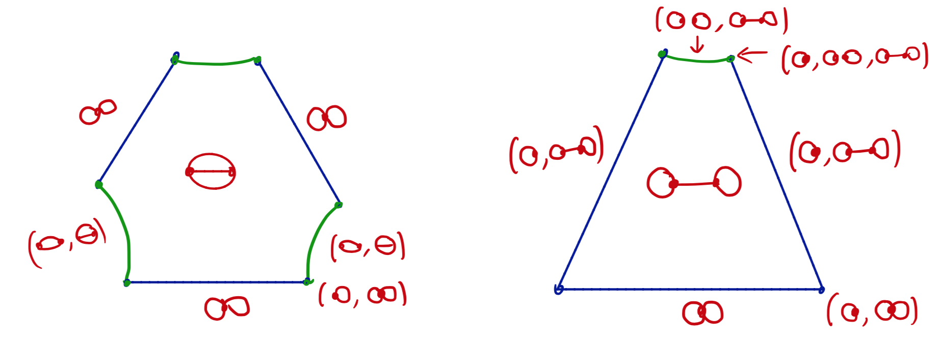
Figure 9. A picture of $|L\mathcal{M}_{2}^{\mathrm{trop},\mathcal{B}}|$. Faces with isomorphic labels are to be identified.

8. The strict transform of the graph locus in $L\mathcal{M}_{g}^{\mathrm{trop},\mathcal{B}}$

Let $G$ be a graph with zero weights. Recall that $\pi_{\mathcal{B}}:P^{\mathcal{B}}_{G}\rightarrow\mathbb{P}^{E_{G}}$ is the corresponding blow-up and $X_{G}\subset\mathbb{P}^{E_{G}}$ is the graph hypersurface. Denote its strict transform by

$$\widetilde{X}_{G}\subset P^{\mathcal{B}_{G}}$$

and let $U_{G}\subset P^{\mathcal{B}_{G}}$ denote its open complement $P^{\mathcal{B}_{G}}\backslash\widetilde{X}_{G}$. Recall from theorem 7.3 that $\left(\mathcal{C}^{\mathcal{B}}_{G}\right)^{\mathrm{opp}}$ is equivalent to the category of faces of the blown-up Feynman polytope $\mathcal{F}^{\mathcal{B}}_{G}$.

Definition 8.1.

Define a functor

$$\widetilde{\mathcal{X}}:\left(\mathcal{C}^{\mathcal{B}}_{G}\right)^{\mathrm{opp}}\longrightarrow\mathrm{Sch}_{\mathbb{Q}}$$

which sends the singleton $(G)$ to the strict transform $\widetilde{X}_{G}\subset P^{\mathcal{B}_{G}}$. It is uniquely defined on all other objects (7.3) by restriction to faces and defines a subscheme functor of $\mathsf{S}\mathcal{F}^{\mathcal{B}}$.

An isomorphism of graphs (or nested sequence of graphs) induces an isomorphism of graph hypersurfaces and hence of their strict transforms by proposition 5.2 (i). Since $I^{\mathcal{B}}_{g}$ is generated by stable unweighted graphs of genus $g$, we deduce the existence of a functor

$$\widetilde{\mathcal{X}}:\left(I^{\mathcal{B}}_{g}\right)^{\mathrm{opp}}\longrightarrow\mathrm{Sch}_{\mathbb{Q}}$$

which is a subscheme functor of $L\mathcal{M}_{g}^{\mathrm{trop},\mathcal{B}}$.

Proposition 8.2.

The functor $\widetilde{\mathcal{X}}:\left(I^{\mathcal{B}}_{g}\right)^{\mathrm{opp}}\rightarrow\mathrm{Sch}_{\mathbb{Q}}$ is given on sequences (7.3) by

(8.1) $$(\gamma_{1},\ldots,\gamma_{n})\ \mapsto\ \bigcup_{i=1}^{n}P^{\gamma_{1}}\times\ldots\times P^{\gamma_{i-1}/\gamma_{i-2}}\times\widetilde{X}_{\gamma_{i}/\gamma_{i-1}}\times P^{\gamma_{i+1}/\gamma_{i}}\times\ldots\times P^{\gamma_{n}/\gamma_{n-1}}$$

where we write $\gamma_{0}=\emptyset$. It is a closed subscheme of $L\mathcal{M}_{g}^{\mathrm{trop},\mathcal{B}}$ at infinity, i.e., a subscheme of the functor $\mathsf{S}L\mathcal{M}_{g}^{\mathrm{trop},\mathcal{B}}$, whose real points do not meet the topological realisation:

(8.2) $$\widetilde{\mathcal{X}}(\mathbb{R})\cap|L\mathcal{M}_{g}^{\mathrm{trop},\mathcal{B}}|=\emptyset\ .$$

The blow-down $(\phi,\Phi):L\mathcal{M}_{g}^{\mathrm{trop},\mathcal{B}}\rightarrow L\mathcal{M}_{g}^{\mathrm{trop}}$ induces a natural transformation $\widetilde{\mathcal{X}}\rightarrow\mathcal{X}\circ\phi$, where $\phi$ is the collapsing functor.

Proof.

If $e\in E_{G}$ is not a tadpole, there is a canonical inclusion $\widetilde{X}_{G/e}\rightarrow\widetilde{X}_{G}$ induced by the inclusion $P_{G/e}^{\mathcal{B}}\rightarrow P_{G}^{\mathcal{B}}$, since this is true for graph hypersurfaces and strict transforms are functorial (proposition 5.2 (i)). This proves the formula (8.1) for sequences of length $n=1$.

The general case follows by taking refinements. Let $\gamma\subset G$ be a core subgraph of $G$. One has the following identity of graph polynomials [BEK06, Bro17a],

$$\Psi_{G}=\Psi_{\gamma}\Psi_{G/\gamma}+R_{G/\gamma}$$

where $R_{G/\gamma}$ is a polynomial of homogeneous degree strictly greater than $\deg\Psi_{\gamma}=h_{\gamma}$ in the edge variables $\alpha_{e}$ for $e\in E_{\gamma}$. The identity implies that if $D\subset P^{G}$ is the exceptional divisor corresponding to the blow-up of $\mathbb{P}^{E_{\gamma}}\subset\mathbb{P}^{E_{G}}$ one has a canonical isomorphism:

$$\widetilde{X}_{G}\cap D\cong\left(\widetilde{X}_{\gamma}\times P^{\mathcal{B}}_{G/\gamma}\right)\ \cup\ \left(P^{\mathcal{B}}_{\gamma}\times\widetilde{X}_{G/\gamma}\right)\ .$$

The fact that $\widetilde{\mathcal{X}}$ is at infinity follows from the fact that the strict transform locus $\widetilde{X}_{G}(\mathbb{R})$ does not meet the region $\sigma^{\mathcal{B}}_{G}$ [BEK06, Bro17a]. The final statement follows by definition from the fact that $X_{G}$ is the blow-down of $\widetilde{X}_{G}$. ∎

The properties of graph hypersurfaces required in the proof will actually be rederived in §11 from a more conceptual viewpoint via properties of the determinant.

The open complement of the subscheme $\widetilde{\mathcal{X}}$ is the functor

$$\mathcal{U}:\left(I^{\mathcal{B}}_{g}\right)^{\mathrm{opp}} \longrightarrow \mathrm{Sch}_{\mathbb{Q}}$$

$$(\gamma_{1},\ldots,\gamma_{n})\ \mapsto \ U(\gamma_{1})\times U(\gamma_{2}/\gamma_{1})\times\ldots\times U(\gamma_{n}/\gamma_{n-1})$$

It is an open subscheme of $\mathsf{S}L\mathcal{M}_{g}^{\mathrm{trop},\mathcal{B}}$ and satisfies $|L\mathcal{M}_{g}^{\mathrm{trop},\mathcal{B}}|\subset\mathcal{U}$ (definition 2.6).

Corollary 8.3.

Via definition 2.7 we deduce a functor

$$L\mathcal{M}_{g}^{\mathrm{trop},\mathcal{B}}\backslash\widetilde{\mathcal{X}}\ :\ \left(I_{g}^{\mathcal{B}}\right)^{\mathrm{opp}} \longrightarrow \mathcal{PC}_{\mathbb{Q}}$$

$$x \mapsto (\mathcal{U}_{x},L^{\mathcal{B}}\cap\mathcal{U}_{x},\sigma_{x})$$

Remark 8.4.

A functorial system of linear subspaces of $\mathsf{S}\mathcal{F}(G)$ was defined in [Bro17a, §5.4] whose complement in $P^{G}$ is affine. It defines a subscheme functor $\mathcal{A}\subset L\mathcal{M}_{g}^{\mathrm{trop},\mathcal{B}}$ such that $\left|L\mathcal{M}_{g}^{\mathrm{trop},\mathcal{B}}\right|\subset P^{G}\backslash\mathcal{A}$. It would be very interesting to construct natural differential forms on $P^{G}\backslash\mathcal{A}$. They would have linear poles (by contrast with the canonical forms studied here.)

8.1. The boundary and open locus

Definition 8.5.

Let $\partial I_{g}^{\mathcal{B}}$ denote the full subcategory of $I_{g}^{\mathcal{B}}$ whose objects are sequences of graphs $(\gamma_{1},\ldots,\gamma_{n})$ where $n\geq 2$. Denote the restriction of $L\mathcal{M}_{g}^{\mathcal{B}}$ to this category by

$$\partial L\mathcal{M}_{g}^{\mathcal{B}}:\partial I_{g}^{\mathcal{B}}\longrightarrow\mathrm{BLC}_{\mathbb{Q}}\ .$$

We shall call it the boundary locus, or exceptional locus, of $L\mathcal{M}_{g}^{\mathrm{trop},\mathcal{B}}$.

The open locus $|L\mathcal{M}_{g}^{\circ,\mathrm{trop}}|$ embeds canonically into both $|L\mathcal{M}_{g}^{\mathrm{trop}}|$ and $|L\mathcal{M}_{g}^{\mathrm{trop},\mathcal{B}}|$.

Proposition 8.6.

There is a morphism of $\mathcal{PC}_{\mathbb{Q}}$-complexes

$$\partial L\mathcal{M}_{g}^{\mathrm{trop},\mathcal{B}}\longrightarrow\partial L\mathcal{M}_{g}^{\mathrm{trop}}$$

given by the pair $(\phi^{\mathrm{opp}},\pi^{\mathcal{B}})$, where $\phi:\partial I_{g}^{\mathcal{B}}\rightarrow\partial I_{g}$ is the restriction of the collapsing functor, and $\pi^{\mathcal{B}}$ is the canonical blow-down map. In addition, there is a canonical embedding

(8.3) $$\left|L\mathcal{M}_{g}^{\circ,\mathrm{trop}}\right|\overset{\sim}{\longrightarrow}\left|L\mathcal{M}_{g}^{\mathrm{trop},\mathcal{B}}\right|\setminus\left|\partial L\mathcal{M}_{g}^{\mathrm{trop},\mathcal{B}}\right|$$

whose inverse is the blow-down $\left|L\mathcal{M}_{g}^{\mathrm{trop},\mathcal{B}}\right|\setminus\left|\partial L\mathcal{M}_{g}^{\mathrm{trop},\mathcal{B}}\right|\overset{\sim}{\longrightarrow}\left|L\mathcal{M}_{g}^{\mathrm{trop}}\right|\setminus\left|\partial L\mathcal{M}_{g}^{\mathrm{trop}}\right|$.

Proof.

The first part is immediate from the fact that the exceptional locus of $\mathcal{F}^{\mathcal{B}}(G)\rightarrow\mathcal{F}(G)$ corresponds to sequences (7.3) of length $\geq 2$. To prove (8.3), first define the full subcategory $I_{g,w=0}$ of $I_{g}$ consisting of graphs of weight $0$, and consider the functor:

$$\sigma\cap\mathcal{U}:I^{\mathrm{opp}}_{g,w=0} \longrightarrow \mathcal{T}op$$

$$G \mapsto (\sigma\cap\mathcal{U})_{G}=\sigma_{G}\backslash\left(\sigma_{G}\cap(X_{G})(\mathbb{R})\right)\ .$$

Note that $(\sigma\cap\mathcal{U})_{G}$ is contained in $\sigma_{G}$, but strictly contains $\overset{\circ}{\sigma}_{G}$. It follows from proposition 6.7 and the fact that $(\sigma\cap\mathcal{U})_{G}$ is the empty set if $w(G)>0$ that:

$$\left|\sigma\cap\mathcal{U}\right|=\varinjlim_{G\in I^{\mathrm{opp}}_{g,w=0}}\sigma_{G}\backslash\left(\sigma_{G}\cap(X_{G})(\mathbb{R})\right)=\left|L\mathcal{M}_{g}^{\circ,\mathrm{trop}}\right|\ .$$

Now consider the functor $\sigma\backslash\mathcal{E}:I_{g}^{\mathcal{B}}\rightarrow\mathcal{T}op$ which sends sequences (7.3) of length $>1$ to the empty set, and maps singletons $(G)$ to

$$(G)\ \mapsto\ (\sigma\backslash\mathcal{E})_{G}=\sigma^{\mathcal{B}}_{G}\ \backslash\ \left(\sigma^{\mathcal{B}}_{G}\cap\mathcal{E}_{G}(\mathbb{R})\right)$$

where $\mathcal{E}_{G}\subset P_{G}^{\mathcal{B}}$ is the exceptional divisor of $\pi_{\mathcal{B}}:P_{G}^{\mathcal{B}}\rightarrow\mathbb{P}^{E_{G}}$. The blow-down morphism defines a functorial isomorphism of algebraic varieties, and of topological spaces:

$$\pi_{G}^{\mathcal{B}}\ :\ P_{G}^{\mathcal{B}}\backslash\left(\mathcal{E}_{G}\cup\widetilde{\mathcal{X}}_{G}\right) \overset{\sim}{\longrightarrow} \mathbb{P}^{E_{G}}\backslash X_{G}$$

$$\sigma^{\mathcal{B}}_{G}\ \backslash\ \left(\sigma^{\mathcal{B}}_{G}\cap\mathcal{E}_{G}(\mathbb{R})\right) \overset{\sim}{\longrightarrow} \sigma_{G}\backslash(\sigma_{G}\cap X_{G})=(\sigma\cap\mathcal{U})_{G}$$

The second line follows from restriction of the first, since $\widetilde{\mathcal{X}}_{G}(\mathbb{R})$ does not meet $\sigma^{\mathcal{B}}_{G}$ by (8.2). Let $j:\sigma_{G}\backslash(\sigma_{G}\cap X_{G})\overset{\sim}{\rightarrow}\sigma^{\mathcal{B}}_{G}\ \backslash\ \left(\sigma^{\mathcal{B}}_{G}\cap\mathcal{E}_{G}(\mathbb{R})\right)$ denote its inverse. To define the continuous map (8.3) we define a pair consisting of a functor and natural transformation, and take its limit. The natural transformation is given by $j$; the functor is given by

$$\iota:I_{g,w=0}\longrightarrow I_{g}^{\mathcal{B}}\qquad\hbox{where}\qquad\iota:G\mapsto(G)\ ,$$

and $(G)$ denotes a sequence of graphs of length one. The isomorphism $j$, which is functorial, thus defines a natural transformation from $\sigma\cap\mathcal{U}$ to

$$(\sigma\backslash\mathcal{E})\circ\iota:I_{g,w=0}\overset{\iota}{\longrightarrow}I_{g}^{\mathcal{B}}\overset{\sigma\backslash\mathcal{E}}{\longrightarrow}\mathcal{T}op$$

It induces a continuous map

$$\left|\sigma\cap\mathcal{U}\right|\longrightarrow\left|\sigma\backslash\mathcal{E}\right|=\varinjlim_{G\in(I_{g}^{\mathcal{B}})^{\mathrm{opp}}}\sigma^{\mathcal{B}}_{G}\ \backslash\ \left(\sigma^{\mathcal{B}}_{G}\cap\mathcal{E}_{G}(\mathbb{R})\right)$$

which is exactly (8.3). The last statement follows from the fact that the inverse of the continuous map $j$ is, by definition, the restriction of the blow-down map $\pi^{\mathcal{B}}$. ∎

The key point in the previous proposition is that simplices which are glued together in the tropical moduli space, and which are not contained in the graph hypersurface locus, continue to be glued together after blowing-up (i.e., if $\mathcal{F}(\gamma)$ is a common face of both $\mathcal{F}(G_{1})$ and $\mathcal{F}(G_{2})$ and $w(\gamma)>0$, then $\mathcal{F}^{\mathcal{B}}(\gamma)$ is a common face of both $\mathcal{F}^{\mathcal{B}}(G_{1})$ and $\mathcal{F}^{\mathcal{B}}(G_{2})$). This is expressed by the fact that $\iota$ is a functor, using the fact that core graphs are intrinsic.

8.2. The face complex associated to $L\mathcal{M}_{g}^{\mathrm{trop},\mathcal{B}}$

Using the general definition 3.1, we may write down the face complex associated to $L\mathcal{M}_{g}^{\mathrm{trop},\mathcal{B}}$.

Definition 8.7.

Let $\mathcal{GC}_{0}^{\mathcal{B}}$ denote the $\mathbb{Q}$-vector space generated by symbols $\big{[}\underline{\Gamma},\omega\big{]}$

$$\hbox{where }\quad\underline{\Gamma}=(\gamma_{1},\ldots,\gamma_{n})\ ,\quad\hbox{ and }\quad\omega=\omega_{\gamma_{1}}\wedge\omega_{\gamma_{2}/\gamma_{1}}\wedge\ldots\wedge\omega_{\gamma_{n}/\gamma_{n-1}}\ ,$$

where $\gamma_{1}\subsetneq\ldots\subsetneq\gamma_{n}$ is a strict nested sequence of graphs where $\gamma_{i}$ is core for $i<n$ and $\gamma_{n}$ stable (definition 7.2), and $\omega_{\gamma_{i+1}/\gamma_{i}}$ is an orientation on the quotients $\gamma_{i+1}/\gamma_{i}$, with relations:

$${[}\underline{\Gamma},-\omega]=-[\underline{\Gamma},\omega]\qquad\hbox{ and }\qquad{[}\underline{\Gamma},\omega]=[\underline{\Gamma}^{\prime},\omega^{\prime}]$$

whenever $\underline{\Gamma}\cong\underline{\Gamma}^{\prime}$ is an isomorphism of nested sequences $f:\gamma_{n}\cong\gamma_{n}^{\prime}$ such that $f(\gamma_{i})=\gamma^{\prime}_{i}$, and $\omega^{\prime}=f(\omega)$. It is bigraded by genus, and edge number. The differential

$$d:\mathcal{GC}_{0}^{\mathcal{B}}\longrightarrow\mathcal{GC}_{0}^{\mathcal{B}}$$

has two components: $d=d^{i}+d^{e}$, which we call the internal and exceptional differentials, respectively. The internal differential is defined by edge contraction (7.4)

$$d^{i}\big{[}(\gamma_{1},\ldots,\gamma_{n}),\omega\big{]}=\sum_{e\in E_{\gamma_{j}/\gamma_{j-1}}}(-1)^{j}\big{[}(\gamma_{1},\ldots,\gamma_{n})/e,\omega^{\prime}\big{]}$$

where the sum is over all admissible edges, $j$ is the unique index such that $e\in E_{\gamma_{j}/\gamma_{j-1}}$ and

$$\omega^{\prime}=\varepsilon\,\omega_{\gamma_{1}}\wedge\ldots\wedge\omega_{\gamma_{i-1}/\gamma_{i-2}}\wedge\omega^{\prime}_{\gamma_{i}/\gamma_{i-1}}\wedge\ldots\wedge\omega_{\gamma_{n}/\gamma_{n-1}}$$

where $\varepsilon=\pm 1$ is defined by $\omega^{\prime}_{\gamma_{i}/\gamma_{i-1}}=\varepsilon\,e\wedge\omega_{\gamma_{i}/(\gamma_{i-1}\cup e)}$. The exceptional differential is:

$$d^{e}\big{[}(\gamma_{1},\ldots,\gamma_{n}),\omega\big{]}=\sum_{\gamma}(-1)^{i}\big{[}(\gamma_{1},\ldots,\gamma_{i-1},\gamma,\gamma_{i},\ldots,\gamma_{n}),\omega^{\prime}\big{]}$$

where the sum is over all refinements for $1\leq i\leq n$, where

$$\omega^{\prime}=\varepsilon\,\omega_{\gamma_{1}}\wedge\ldots\wedge\omega_{\gamma_{i-1}/\gamma_{i-2}}\wedge\omega^{\prime}_{\gamma/\gamma_{i-1}}\wedge\omega^{\prime}_{\gamma_{i}/\gamma}\wedge\ldots\wedge\omega_{\gamma_{n}/\gamma_{n-1}}$$

and where $\varepsilon=\pm 1$ is defined by $\omega_{\gamma_{i}/\gamma_{i-1}}=\varepsilon\omega^{\prime}_{\gamma/\gamma_{i-1}}\wedge\omega^{\prime}_{\gamma_{i}/\gamma}$.

The complex $\mathcal{GC}_{0}^{\mathcal{B}}$ is filtered by the length $n$ of sequences. Let $F_{k}\mathcal{GC}_{0}^{\mathcal{B}}$ denote the subcomplex whose generators $[(\gamma_{1},\ldots,\gamma_{n}),\omega]$ have $n>k$ components.

Proposition 8.8.

If we write $\mathcal{GC}_{0}^{\partial\mathcal{B}}=F_{1}\mathcal{GC}_{0}^{\mathcal{B}}$ then

$$H_{n}(\mathcal{GC}_{0}^{\mathcal{B}})\cong H_{n-1}(\left|L\mathcal{M}_{g}^{\mathrm{trop},\mathcal{B}}\right|)\quad\hbox{ and }\quad H_{n}(\mathcal{GC}_{0}^{\partial\mathcal{B}})\cong H_{n-1}(\left|\partial L\mathcal{M}_{g}^{\mathrm{trop},\mathcal{B}}\right|)\ .$$

Furthermore, the homology of the usual commutative even graph complex satisfies $H_{n}(\mathcal{GC}_{0})=H_{n}(\mathcal{GC}_{0}^{\mathcal{B}},\mathcal{GC}_{0}^{\partial\mathcal{B}})$ and fits into a long exact sequence

$$\ldots\longrightarrow H_{n}(\mathcal{GC}_{0}^{\partial\mathcal{B}})\longrightarrow H_{n}(\mathcal{GC}_{0}^{\mathcal{B}})\longrightarrow H_{n}(\mathcal{GC}_{0})\overset{d^{e}}{\longrightarrow}H_{n-1}(\mathcal{GC}_{0}^{\partial\mathcal{B}})\longrightarrow\ldots$$

Proof.

This follows from theorem 3.2, the relative long exact homology sequence, and (8.3) to identify $H_{n}(\left|L\mathcal{M}_{g}^{\mathrm{trop},\mathcal{B}}\right|,\left|\partial L\mathcal{M}_{g}^{\mathrm{trop},\mathcal{B}}\right|)=H_{n}(\left|L\mathcal{M}_{g}^{\mathrm{trop}}\right|,\left|\partial L\mathcal{M}_{g}^{\mathrm{trop}}\right|)$. ∎

9. Polyhedra in spaces of quadratic forms

We now turn to the study of polyhedra whose vertices are positive semi-definite quadratic forms with rational null spaces.

9.1. Positive semi-definite matrices

Let $\mathcal{P}_{g}$ denote the space of positive definite $g\times g$ real symmetric matrices. It may be identified, via the map $X\mapsto X^{T}X$, with $\mathrm{GL}_{g}(\mathbb{R})/O_{g}(\mathbb{R})$, and admits a right action $M\mapsto h^{T}Mh$ for $h\in\mathrm{GL}_{g}(\mathbb{R})$. We write $L\mathcal{P}_{g}=\mathcal{P}_{g}/\mathbb{R}^{\times}_{>0}$.

The space of real non-zero symmetric matrices up to scalar multiplication may be identified with the real points of the projective space $\mathbb{P}^{d_{g}-1}$, where $d_{g}=\binom{g+1}{2}$, and hence $L\mathcal{P}_{g}\subset\mathbb{P}^{d_{g}-1}(\mathbb{R})$. A choice of homogeneous coordinates on $\mathbb{P}^{d_{g}-1}$ are given by matrix entries on or above the diagonal. Since the determinant is a homogeneous function of these coordinates, its vanishing locus defines a hypersurface

$$\mathrm{Det}\ \subset\ \mathbb{P}^{d_{g}-1}\$$

which satisfies $L\mathcal{P}^{g}\cap\mathrm{Det}(\mathbb{R})=\emptyset$. The linear action of $\mathrm{GL}_{g}$ on $\mathbb{P}^{d_{g}-1}$, which corresponds to the action $M\mapsto h^{T}Mh$ on symmetric matrices, preserves $\mathrm{Det}$ and $L\mathcal{P}_{g}\subset\mathbb{P}^{d_{g}-1}(\mathbb{R})$.

9.2. Positive polyhedra in the space of symmetric matrices

It is convenient to reformulate the above in a coordinate-free manner. Consider a vector space $V$ of dimension $g$ defined over a field $k\subset\mathbb{R}$. Let us denote by

$$\mathcal{Q}(V)=\left(\mathrm{Sym}^{2}\,V\right)^{\vee}$$

the $k$-vector space of symmetric bilinear (i.e., quadratic) forms

$$Q:V\otimes_{k}V\longrightarrow k\ .$$

Such a quadratic form may be viewed as a linear map $Q:V\rightarrow V^{\vee}$ which is self-dual, i.e., $Q=Q^{T}$. Consequently, $\mathcal{Q}$ defines a contravariant functor from the category of vector spaces to itself: for any linear map $V\rightarrow W$, there is a natural map $\mathcal{Q}(W)\rightarrow\mathcal{Q}(V)$. It sends surjective maps to injective maps, and vice-versa. Given an isomorphism $V\cong k^{g}$ one may identify elements of $\mathcal{Q}(V)$ with symmetric matrices with entries in $k$.

Recall that the null space $\ker(Q)$ of a quadratic form is defined to be the kernel of $Q:V\rightarrow V^{\vee}$. If $Q$ is a positive semi-definite quadratic form, one has

(9.1) $$Q(v,v)=0\quad\Longleftrightarrow\quad v\in\mathrm{ker}(Q)\ .$$

Consider the projective space $\mathbb{P}(\mathcal{Q}(V))$. It has distinguished linear subspaces:

$$\mathbb{P}(\mathcal{Q}(V/K))\lhook\joinrel\rightarrow\mathbb{P}(\mathcal{Q}(V))\qquad\hbox{ for every }K\subset V\ .$$

Such a subspace is contained in the determinant locus $\mathrm{Det}\subset\mathbb{P}(\mathcal{Q}(V))$ if and only if $K\neq 0$. Viewing $\mathcal{Q}(V/K)$ as the subspace of $\mathcal{Q}(V)$ of quadratic forms $Q$ satisfying $Q(k,v)=0$ for all $k\in K$, and $v\in V$, one deduces the formula:

(9.2) $$\mathcal{Q}\left(V/K_{1}\right)\cap\mathcal{Q}\left(V/K_{2}\right)=\mathcal{Q}\left(V/(K_{1}+K_{2})\right)$$

which implies that $\mathbb{P}\left(\mathcal{Q}\left(V/K_{1}\right)\right)\cap\mathbb{P}\left(\mathcal{Q}\left(V/K_{2}\right)\right)=\mathbb{P}\left(\mathcal{Q}\left(V/(K_{1}+K_{2})\right)\right)$.

Consider the convex subsets

$$\mathcal{Q}^{>0}(V)\ \subset\ \mathcal{Q}^{\geq 0}(V)\ \subset\ \mathcal{Q}(V)$$

consisting of positive definite, and positive semi-definite, quadratic forms on $V$.

Definition 9.1.

We shall say that a polyhedron $(\sigma,\mathcal{Q}(V))$ in the space of quadratic forms is positive, which we shall denote by $\sigma\geq 0$, if its vertices lie in $\mathcal{Q}^{\geq 0}(V)$, and hence $\sigma\subset\mathcal{Q}^{\geq 0}(V)(\mathbb{R})$ is contained in the set of positive semi-definite quadratic forms.

We shall call a polyhedron strictly positive, denoted by $\sigma>0$, if $\sigma$ positive, and if in addition it meets the interior $\sigma\cap\mathcal{Q}^{>0}(V)\neq\emptyset$. In other words, $\sigma$ is strictly positive if it contains at least one positive definite quadratic form.

Positive polyhedra meet the determinant locus in a specific manner.

Lemma 9.2.

Let $\sigma$ be a positive polyhedron in $\mathcal{Q}(V)$ and let $\sigma_{F}$ be a face of $\sigma$ of dimension $>0$. The following are equivalent:

(i) The face $\sigma_{F}$ is contained in the determinant locus $\mathrm{Det}(\mathbb{R})$.

(ii) There is a point in the interior of $\sigma_{F}$ which lies in $\mathrm{Det}(\mathbb{R})$, i.e.,

$$\overset{\circ}{\sigma}_{F}\cap\mathrm{Det}(\mathbb{R})\neq\emptyset$$

(iii) There is a non-zero linear subspace $0\neq K\subset V$ such that

$$\sigma_{F}\ \subset\ \mathbb{P}(\mathcal{Q}(V/K))(\mathbb{R})\ .$$

Proof.

Clearly $(i)$ implies $(ii)$ and $(iii)$ imples $(i)$ since $\mathbb{P}(\mathcal{Q}(V/K))\subset\mathrm{Det}$. It suffices to prove that $(ii)$ implies $(iii)$. Let us write $\widehat{\sigma}_{F}=\{\sum_{i=1}^{n}\lambda_{i}Q_{i}:\lambda_{i}\in\mathbb{R}_{\geq 0}\}$ where $Q_{i}$ are non-zero positive semi-definite quadratic forms on $V$. If we assume $(ii)$ then there exist $\lambda_{i}>0$ such that $\det\left(\sum_{i=1}^{n}\lambda_{i}Q_{i}\right)=0$ since every interior point of $\sigma$ admits a (non-unique) representation as a linear combination of $Q_{i}$ with strictly positive coefficients. Therefore there is a non-zero vector $x\in V$ such that $x\in\mathrm{ker}\left(\sum_{i=1}^{n}\lambda_{i}Q_{i}\right)$. This implies in particular that $\sum_{i=1}^{n}\lambda_{i}Q_{i}(x,x)=0$. Since $Q_{i}(x,x)\geq 0$ we deduce that $Q_{i}(x,x)=0$ for all $i=1,\ldots,n$. By (9.1), $x\in\ker Q_{i}$ for all $i$. If we set $K_{\sigma_{F}}=\bigcap_{i=1}^{n}\ker(Q_{i})$, then $x\in K_{\sigma_{F}}$, and in particular $K_{\sigma_{F}}\neq 0$. Property $(iii)$ holds on setting $K=K_{\sigma_{F}}$. ∎

It follows that if $\sigma\geq 0$ is a positive polyhedron, then it is strictly positive if and only if its interior does not meet the determinant locus:

(9.3) $$\sigma>0\quad\Longleftrightarrow\quad\overset{\circ}{\sigma}\cap\mathrm{Det}(\mathbb{R})=\emptyset\ .$$

Definition 9.3.

For any positive polyhedron $\sigma\geq 0$ in $\mathbb{P}(\mathcal{Q}(V))$, we denote by $K_{\sigma}\subset V$ the common null space of its vertices.

It follows from (9.2) that $K_{\sigma}$ is the unique largest subspace of $V$ such that

$$\sigma\ \subset\ \mathbb{P}(\mathcal{Q}(V/K_{\sigma}))(\mathbb{R})\ .$$

In particular, $\sigma$ meets the strictly positive locus, i.e., $\sigma\cap\mathcal{Q}^{>0}(V/K_{\sigma})\neq\emptyset$ and thus the polyhedron $(\sigma,V/K_{\sigma})$ is strictly positive.

Lemma 9.4.

Let $\sigma\geq 0$ be a positive polyhedron. For any subspace $K\subset V$,

$$\sigma\cap\mathbb{P}(\mathcal{Q}(V/K))(\mathbb{R})$$

is either empty, or is a face of $\sigma$.

Proof.

For every $v\in K$, consider the linear map $f_{v}:\mathcal{Q}(V)\rightarrow k$ defined by $Q\mapsto Q(v,v).$ Its kernel is $\mathcal{Q}(V/kv)$, which contains $\mathcal{Q}(V/K)$ by definition. The linear form $f_{v}$ is non-negative on the subspace $\mathcal{Q}^{\geq 0}(V)\subset\mathcal{Q}(V)$. It follows from (9.2) that, for any vectors $v_{1},\ldots,v_{d}$ which span $K$, one has $\mathcal{Q}(V/K)=\bigcap_{i=1}^{d}\mathcal{Q}(V/kv_{i})=\bigcap_{i=1}^{d}H_{i}$, where $H_{i}=\ker(f_{v_{i}})$. Since $f_{v_{i}}$ is non-negative on $\sigma$, the set $\sigma\cap\mathbb{P}(H_{i})$ is either empty, or a face of $\sigma$, and

$$\sigma\cap\mathbb{P}(V/K)(\mathbb{R})=\bigcap_{i=1}^{d}\sigma\cap H_{i}(\mathbb{R})$$

is either empty or a non-empty intersection of faces of $\sigma$ and hence also a face. ∎

The previous lemma has the important consequence that in defining $L\mathcal{A}_{g}^{\mathrm{trop},\mathcal{B}}$ we shall only need to blow up linear subspaces of $\mathbb{P}(\mathcal{Q}(V))$ of the special form $\mathbb{P}(\mathcal{Q}(V/K))$.

Definition 9.5.

For any face $\sigma_{F}$ of $\sigma$, define its essential envelope to be the face

$$\sigma_{F}^{\mathrm{ess}}=\left(\sigma\cap\mathbb{P}(\mathcal{Q}(V/K_{\sigma_{F}}))(\mathbb{R})\right)\ .$$

It satisfies $\sigma_{F}\subset\sigma_{F}^{\mathrm{ess}}$. We call a face $\sigma_{F}$ essential if $\sigma_{F}=\sigma^{\mathrm{ess}}_{F}$.

If $\sigma_{F}>0$ is strictly positive, then $K_{\sigma_{F}}=0$ and one has $\sigma^{\mathrm{ess}}_{F}=\sigma$. In general, a face $\sigma_{F}$ of $\sigma_{Q}$ (whether essential or not) will not be Zariski dense in $\mathbb{P}^{Q}\cap\mathbb{P}(\mathcal{Q}(V/K_{\sigma}))$. Proposition 12.5 implies that for Feynman polytopes, the essential envelope of a face $\sigma_{G/\gamma}$ indexed by a subgraph $\gamma\subset G$ is the face $\sigma_{G/\gamma^{\mathrm{core}}}$ where $\gamma^{\mathrm{core}}\subset\gamma$ is the maximal core subgraph of $\gamma$.

Lemma 9.6.

The intersection of an essential face of $\sigma$ with any other face $\sigma_{Q^{\prime}}$ of $\sigma$, is either empty or another essential face of $\sigma_{Q^{\prime}}$.

Proof.

The set of essential faces of $\sigma$ are precisely the sets $\sigma\cap\mathbb{P}(\mathcal{Q}(V/K))(\mathbb{R})$ where $K\subset V$ is a linear subspace. The intersection of such a face with $\sigma_{Q^{\prime}}$ is $\sigma_{Q^{\prime}}\cap\mathbb{P}(\mathcal{Q}(V/K))(\mathbb{R})$, which is therefore also essential or empty. ∎

9.3. Collapsing the complement of the determinant in the normal bundle

Restriction of quadratic forms to any subspace $K\subset V$ defines a linear map:

(9.4) $$\mathcal{Q}(V)/\mathcal{Q}(V/K)\longrightarrow\mathcal{Q}(K)\ .$$

It does not induce a map on the corresponding projective spaces since it is not injective in general. To see this, choose a complementary space $V\cong K\oplus C$ where $C\cong V/K$. The space $\mathcal{Q}(V)/\mathcal{Q}(V/K)$ may be represented by symmetric matrices in block matrix form,

(9.5) $$Q=\left(\begin{array}[]{c|c}Q_{0}&Q_{1}\\ \hline\cr Q_{1}^{T}&0\end{array}\right)\ ,$$

which implies that $\mathcal{Q}(V)/\mathcal{Q}(V/K)$ is isomorphic to the product $\mathcal{Q}(K)\times\mathbb{A}^{\mathrm{Hom}(V/K,K)}$. The map $\mathcal{Q}(V)/\mathcal{Q}(V/K)\rightarrow\mathcal{Q}(K)$ sends $Q\mapsto Q_{0}$. The determinant function $\det:\mathcal{Q}(K)\rightarrow k$ defines a homogeneous polynomial

$$Q\mapsto\det(Q\big{|}_{K})\ :\ \mathcal{Q}(V)/\mathcal{Q}(V/K)\longrightarrow k\ .$$

In the coordinates $\eqref{QBlockform}$, $\det(Q\big{|}_{K})$ is simply $\det(Q_{0})$. Denote its zero locus by

(9.6) $$\mathrm{Det}\big{|}_{K}\ \subset\ \mathbb{P}\left(\mathcal{Q}(V)/\mathcal{Q}(V/K)\right)\ .$$

Lemma 9.7.

Restriction of quadratic forms to $K$ gives a well-defined projection

(9.7) $$\pi_{K}\ :\ \mathbb{P}\left(\mathcal{Q}(V)/\mathcal{Q}(V/K)\right)\ \setminus\ \mathrm{Det}\big{|}_{K}\longrightarrow\mathbb{P}\left(\mathcal{Q}(K)\right)\ \setminus\ \mathrm{Det}_{K}$$

which is a fibration in affine spaces $\mathrm{Hom}(V/K,K)\cong\mathbb{A}^{\dim K.\dim V/K}$. It is functorial, i.e., for any $h\in\mathrm{GL}(V)$, there is a commutative diagram:

$$\begin{array}[]{ccc}\mathbb{P}\left(\mathcal{Q}(V)/\mathcal{Q}(V/K)\right)\ \setminus\ \mathrm{Det}\big{|}_{K}&\overset{\pi_{K}}{\longrightarrow}&\mathbb{P}\left(\mathcal{Q}(K)\right)\ \setminus\ \mathrm{Det}_{K}\\ \downarrow&&\downarrow\\ \mathbb{P}\left(\mathcal{Q}(V)/\mathcal{Q}(V/K^{\prime})\right)\ \setminus\ \mathrm{Det}\big{|}_{K^{\prime}}&\overset{\pi_{K^{\prime}}}{\longrightarrow}&\mathbb{P}\left(\mathcal{Q}(K^{\prime})\right)\ \setminus\ \mathrm{Det}_{K^{\prime}}\end{array}$$

where the vertical maps are isomorphisms $Q\mapsto h^{T}Qh$ and $K^{\prime}=h^{T}Kh$.

Proof.

A choice of decomposition (9.5) defines projective coordinates on $\mathbb{P}\left(\mathcal{Q}(V)/\mathcal{Q}(V/K)\right)$. The complement of $\mathrm{Det}\big{|}_{K}$ consists of projective classes of matrices with $\det(Q_{0})\neq 0$. In particular, $Q_{0}\neq 0$ and so the map $Q\mapsto Q_{0}$ is well-defined on projective spaces. Its fiber is isomorphic to the space of matrices $Q_{1}$, which is nothing other than the vector space $\mathrm{Hom}(V/K,K)$, viewed as the $k$ points of an affine space of equal dimension. ∎

Note that the ambiguity in the choice of decomposition $V\cong K\oplus V/K$, is the set of splittings of the exact sequence $0\rightarrow K\rightarrow V\rightarrow V/K\rightarrow 0$, which is a torsor over $\mathrm{Hom}(V/K,K)$.

9.4. Strict positivity of normal faces

For simplicity of notation, let us write

(9.8) $$\sigma/\sigma_{F}=\sigma_{/K_{\sigma_{F}}}$$

for the normal polyhedron (definition 4.8) of $\sigma$ relative to the null space $K_{\sigma_{F}}$ of a face $\sigma_{F}$.

Lemma 9.8.

Let $\sigma$ be strictly positive and let $\sigma_{F}$ be a face of $\sigma$. In the product

$$\sigma_{F}\times\left(\sigma/\sigma_{F}\right)\ \subset\ \mathbb{P}\left(\mathcal{Q}(V/K_{\sigma_{F}})\right)\ \times\ \mathbb{P}\left(\mathcal{Q}(V)/\mathcal{Q}(V/K_{\sigma_{F}})\right)\ ,$$

both $\sigma_{F}$ and $\sigma/\sigma_{F}$ are strictly positive (definition 9.1). In the latter case, this means that the interior of the polyhedron $\sigma/\sigma_{F}$ does not meet the determinant locus:

$$\overset{\circ}{\left(\sigma/\sigma_{F}\right)}\subset\mathbb{P}\left(\mathcal{Q}(V)/\mathcal{Q}(V/K_{\sigma_{F}})\right)\ \setminus\ \mathrm{Det}\big{|}_{K_{\sigma_{F}}}$$

or equivalently, that the image $\pi_{K}(\sigma/\sigma_{F})$ is a positive polyhedron in $\mathbb{P}(\mathcal{Q}(K))$.

Proof.

The vertices of $\sigma$ are projective classes of positive semi-definite quadratic forms $Q_{1},\ldots,Q_{n}\in\mathcal{Q}(V)$. The vertices of the face $\sigma_{F}$ correspond to a subset of them: $\{Q_{i},i\in I\}$, where $I\subset\{1,\ldots,n\}$. By definition,

(9.9) $$K_{\sigma_{F}}=\bigcap_{i\in I}\ker Q_{i}\ ,$$

which implies that in any choice of decomposition $V=K_{\sigma_{F}}\oplus C$, where $C\cong V/K_{\sigma_{F}}$, the matrices $Q_{i}$ have the block matrix form

$$Q_{i}=\left(\begin{array}[]{c|c}0&0\\ \hline\cr 0&\overline{Q}_{i}\end{array}\right)\quad\hbox{ if and only if }\quad i\in I\ ,$$

where the $\overline{Q}_{i}$ are the restrictions of $Q_{i}$ to $K_{\sigma_{F}}$, and are positive semi-definite. Suppose that $\sigma_{F}$ is not strictly positive. Then $\sigma_{F}$ is contained in $\mathrm{Det}_{V/K_{\sigma_{F}}}(\mathbb{R})\subset\mathbb{P}(\mathcal{Q}(V/K_{\sigma_{F}}))(\mathbb{R})$. By lemma 9.2, there is a subspace $0\neq K^{\prime}\subset V/K_{\sigma_{F}}$ which is contained in $\bigcap_{i}\ker\,\overline{Q}_{i}$. But this implies $\bigcap_{i}\ker\,Q_{i}$ is strictly larger than $K_{\sigma_{F}}$, contradicting (9.9).

The polyhedron $\sigma/\sigma_{F}$ has vertices given by the projective classes of the $Q_{j}$, $j\notin I$ which are non-zero in the quotient $\mathcal{Q}(V)/\mathcal{Q}(V/K_{\sigma_{F}})$ and have block matrix representatives

$$Q_{j}=\left(\begin{array}[]{c|c}R_{j}&P_{j}\\ \hline\cr P_{j}^{T}&0\end{array}\right)\quad\hbox{ for all }j\notin I\ .$$

If $\sigma/\sigma_{F}$ were contained in $\mathrm{Det}|_{K_{\sigma_{F}}}(\mathbb{R})$, then by the argument of lemma 9.2 applied to the matrices $R_{j}$, for $j\notin I$, there would exist $0\neq x\in K_{\sigma_{F}}$ such that $x\in\ker(R_{j})\subset K_{\sigma_{F}}$ for all $j\notin I$. In this case, the image $y$ of $x$ in $V$, satisfies $Q_{j}(y,y)=R_{j}(x,x)=0$ and hence $y\in\ker(Q_{j})$ for all $j\notin I$. Since $y\in\ker(Q_{i})$ for all $i\in I$ by (9.9), we deduce that $y$ lies in $\ker\,Q_{i}$, for all $i=1,\ldots,n$, contradicting the strict positivity of $\sigma$ by lemma 9.2. ∎

Remark 9.9.

This lemma easily extends to the case when $\sigma$ is a strictly positive polyhedron in the space $\mathbb{P}(\mathcal{Q}(V)/\mathcal{Q}(V/K))$. The statement is the following: in the product of polyhedra

$$\sigma_{F}\times(\sigma/\sigma_{F})\subset\mathbb{P}\left(\mathcal{Q}(V/K_{\sigma_{F}})/\mathcal{Q}(V/K)\right)\times\mathbb{P}\left(\mathcal{Q}(V)/\mathcal{Q}(V/K_{\sigma_{F}})\right)$$

both $\sigma_{F}$ and $\sigma/\sigma_{F}$ are strictly positive. The proof is identical: one only needs to consider symmetric matrices with a number of initial rows and columns which are identically zero.

9.5. Blow-ups and the determinant locus

The determinant locus is well-behaved with respect to blowing up linear subspaces of the form $\mathbb{P}(\mathcal{Q}(V/K))$.

Proposition 9.10.

Let $0\neq K\subset V$ be a subspace and let

$$\pi:\mathbb{P}\longrightarrow\mathbb{P}(\mathcal{Q}(V))$$

denote the blow-up of $\mathbb{P}(\mathcal{Q}(V))$ along $\mathbb{P}(\mathcal{Q}(V/K))$. The exceptional divisor $\mathcal{E}$ may be canonically identified with the normal bundle of $\mathbb{P}(\mathcal{Q}(V/K))$:

$$\mathcal{E}\cong\mathbb{P}(\mathcal{Q}(V/K))\times\mathbb{P}(\mathcal{Q}(V)/\mathcal{Q}(V/K))\ .$$

If $\widetilde{\mathrm{Det}}_{V}$ denotes the strict transform of the determinant locus, we have

$$\widetilde{\mathrm{Det}}_{V}\cap\mathcal{E}\ \cong\ \left(\mathrm{Det}_{V/K}\times\mathbb{P}(\mathcal{Q}(V)/\mathcal{Q}(V/K))\right)\ \cup\ \left(\mathbb{P}(\mathcal{Q}(V/K))\times\mathrm{Det}\big{|}_{K}\right)\ ,$$

where $\mathrm{Det}\big{|}_{K}$ was defined in (9.6). In particular one has the product formula:

$$\mathcal{E}\ \setminus\ \left(\mathcal{E}\cap\widetilde{\mathrm{Det}}_{V}\right)\ \cong\ \left(\mathbb{P}(\mathcal{Q}(V/K))\ \setminus\ \mathrm{Det}_{V/K}\right)\ \times\ \left(\mathbb{P}(\mathcal{Q}(V)/\mathcal{Q}(V/K))\ \setminus\ \mathrm{Det}\big{|}_{K}\right)\ .$$

Proof.

Choose a complementary space to $K$, i.e., $V\cong K\oplus C$ and choose bases of $K,C$. We can compute the blow up in local affine coordinates (§5.2) as follows. A quadratic form in $Q\in\mathcal{Q}(V)$ may be written in the form

(9.10) $$Q=\begin{pmatrix}Q_{K}&P\\ P^{T}&Q_{C}\end{pmatrix}$$

Let $x_{ij}$ denote the $(i,j)^{\mathrm{th}}$ matrix coefficient. A choice of affine coordinates on $\mathbb{P}(\mathcal{Q}(V))$ is given by the $x_{ij}$ which lie on or above the diagonal $i\leq j$, and one $x_{ij}$ is set to $1$. The locus $\mathbb{P}(\mathcal{Q}(V/K))$ is represented by matrices such that $Q_{K}=P=0$, i.e., the vanishing of $x_{ij}$ for $i\leq j$ such that $i\leq\dim(K)$. In any such local affine coordinates (see §5.2) on this locus (i.e., $x_{i_{0}j_{0}}=1$, where $i_{0}\leq j_{0}$, $i_{0}\leq\dim(K)$) the blow up is represented by the map:

$$s^{*}_{K}:k[x_{ij},i\leq j] \longrightarrow k[z,x_{ij},i\leq j]$$

$$s^{*}_{K}(x_{ij}) = zx_{ij}\quad\hbox{ if }i\leq\dim(K)$$

$$s^{*}_{K}(x_{ij}) = x_{ij}\quad\hbox{ otherwise }$$

The exceptional divisor is defined by the equation $z=0$. Applying the map $s^{*}_{K}$ to the entries of the matrix of a quadratic form (9.10), we obtain

(9.11) $$s_{K}^{*}Q=\begin{pmatrix}zQ_{K}&zP\\ zP^{T}&Q_{C}\end{pmatrix}\ .$$

It follows from the theory of Schur complements that

$$\begin{pmatrix}zQ_{K}&zP\\ zP^{T}&Q_{C}\end{pmatrix}=\begin{pmatrix}I&0\\ P^{T}Q_{K}^{-1}&I\end{pmatrix}\begin{pmatrix}zQ_{K}&0\\ 0&Q_{C}-zP^{T}Q_{K}^{-1}P\end{pmatrix}\begin{pmatrix}I&Q_{K}^{-1}P\\ 0&I\ .\end{pmatrix}$$

in the ring of matrices with coefficients in $k[z,x_{ij},\det(Q_{K})^{-1}]$. The determinants satisfy $\det(s_{K}^{*}Q)=\det(zQ_{K})\det(Q_{C}-zP^{T}Q_{K}^{-1}P)$. This implies that

$$\det(s_{K}^{*}Q)=z^{\dim K}\det(Q_{K})\det(Q_{C})\mod(z^{\dim K+1})\ .$$

It follows that the intersection of the strict transform of the locus $\det(Q)=0$ with the exceptional divisor $z=0$ is given by the equation $\det(Q_{K})\det(Q_{C})=0$. The zero loci of $\det(Q_{K})$ and $\det(Q_{C})$ are $\mathrm{Det}\big{|}_{K}$, and $\mathrm{Det}_{V/K}$ respectively. ∎

This result generalises several asymptotic factorisation theorems for graph polynomials [Bro17a, §2] simply by applying the proposition to a suitable graph Laplacian matrix.

10. Perfect cone compactification

Now consider the case when $k=\mathbb{Q}$ and the vector space $V=V_{\mathbb{Z}}\otimes\mathbb{Q}$ has a lattice $V_{\mathbb{Z}}$. It is convenient to identify $V_{\mathbb{Z}}\cong\mathbb{Z}^{g}$ for the purposes of the ensuing discussion.

10.1. Rational closure of $\mathcal{P}_{g}$

The rational closure $\mathcal{P}^{\mathrm{rt}}_{g}$ of the space of positive definite matrices $\mathcal{P}_{g}$ is defined to be the space of positive semi-definite matrices $M$ whose null space $\ker(M)$ is defined over $\mathbb{Q}$. A positive semi-definite matrix $M$ has rational kernel if and only if there exists an element $h\in\mathrm{GL}_{g}(\mathbb{Z})$ such that

$$h^{T}Mh=\begin{pmatrix}M_{0}&0\\ 0&0\end{pmatrix}$$

where $M_{0}$ is positive definite, i.e., $M_{0}\in\mathcal{P}_{g^{\prime}}$ for some $g^{\prime}\leq g$.

Recall from §9.1 that we identify the space of $g\times g$ matrices with $\mathbb{R}^{d_{g}}$, where $d_{g}=\binom{g+1}{2}$. We have inclusions $\mathcal{P}_{g}\subset\mathcal{P}^{\mathrm{rt}}_{g}\subset\mathbb{R}^{d_{g}}$ and

$$L\mathcal{P}_{g}\subset L\mathcal{P}^{\mathrm{rt}}_{g}\subset\mathbb{P}^{d_{g}-1}(\mathbb{R})$$

where the link of $\mathcal{P}^{\mathrm{rt}}_{g}$ is defined by $L\mathcal{P}^{\mathrm{rt}}_{g}=\left(\mathcal{P}^{\mathrm{rt}}_{g}\setminus\{0\}\right)/\mathbb{R}^{\times}_{>0}$. The group $\mathrm{GL}_{g}(\mathbb{Z})$ preserves all three spaces. One has $L\mathcal{P}^{\mathrm{rt}}_{g}\ \setminus\ L\mathcal{P}_{g}\ \subset\ \mathrm{Det}(\mathbb{R})$.

Remark 10.1.

Lemma 9.2 and the discussion which follows implies that a positive polyhedron $(\sigma,\mathcal{Q}(\mathbb{Q}^{g}))$ has the property that $\sigma$ is contained in the space $\mathcal{P}_{g}^{\mathrm{rt}}$, i.e., every point of $\sigma$ defines a real symmetric matrix with rational kernel.

10.2. Minimal vectors and polyhedral linear configurations

For any positive definite real quadratic form $Q$ on $\mathbb{R}^{g}$, denote its set of minimal vectors by

$$M_{Q}=\{\lambda\in\mathbb{Z}^{g}\setminus\{0\}:Q(\lambda)\leq Q(\mu)\hbox{ for all }\mu\in\mathbb{Z}^{g}\setminus\{0\}\}\ .$$

The associated polyhedral cone is defined to be

$$\widehat{\sigma}_{Q}=\mathbb{R}_{\geq 0}\langle\lambda\lambda^{T}\rangle_{\lambda\in M_{Q}}\subset\mathcal{P}^{\mathrm{rt}}_{g}$$

where the $\lambda\lambda^{T}$ are rank one quadratic forms in $\mathcal{P}^{\mathrm{rt}}_{g}$. The cone $\widehat{\sigma}_{Q}$ is strongly convex since this is already the case for $\mathcal{P}^{\mathrm{rt}}_{g}$ (although $\mathcal{P}^{\mathrm{rt}}_{g}$ is not itself a polyhedral cone). A positive definite quadratic form $Q$ is called perfect if $\widehat{\sigma}_{Q}$ has maximal dimension $d_{g}$. Equivalently, $Q$ is uniquely determined up to a scalar multiple by its set of minimal vectors [Mar03, Vor08].

Definition 10.2.

For any positive definite real quadratic form $Q$ denote by

(10.1) $$\mathsf{c}_{Q}=(\mathbb{P}^{Q},L_{Q},\sigma_{Q})$$

the polyhedral linear configuration where $\sigma_{Q}=L\widehat{\sigma}_{Q}=\left(\widehat{\sigma}_{Q}\backslash\{0\}\right)/\mathbb{R}^{\times}_{>0}$ is the link of $\widehat{\sigma}_{Q}$ in $\mathbb{P}^{d_{g}-1}(\mathbb{R})$, $L_{Q}=\bigcup_{i}L_{i}$ is the union of the Zariski closures of its facets, and $\mathbb{P}^{Q}\subset\mathbb{P}^{d_{g}-1}\cong\mathbb{P}(\mathcal{Q}(V))$ is the linear subspace defined by the Zariski-closure of $\sigma_{Q}$.

The configuration $\mathsf{c}_{Q}$ is thus an object of the category $\mathrm{PLC}_{\mathbb{Q}}$. The form $Q$ is perfect if and only if $\mathbb{P}^{Q}=\mathbb{P}^{d_{g}-1}$, i.e., $\sigma_{Q}$ is Zariski dense in the whole space of quadratic forms.

10.3. Admissible decompositions

See [MBW22, Nam80, FC90, Vor08].

Definition 10.3.

A set $\Sigma=\{\widehat{\sigma}_{i}\}$ of polyhedral cones $\widehat{\sigma}_{i}\subset\mathcal{P}_{g}^{\mathrm{rt}}$ is called admissible if it is stable under the action of $\mathrm{GL}_{g}(\mathbb{Z})$, and such that:

• it covers $\mathcal{P}^{\mathrm{rt}}_{g}$, i.e., $\bigcup_{i}\widehat{\sigma}_{i}=\mathcal{P}^{\mathrm{rt}}_{g},$

• if $\widehat{\sigma}\in\Sigma$, then all the faces of $\widehat{\sigma}$ are elements of $\Sigma$,

• the intersection of two cones in $\Sigma$ is a face of both cones,

• the set of $\mathrm{GL}_{g}(\mathbb{Z})$-orbits of $\Sigma$ is finite.

Theorem 10.4.

(Voronoï). The set of cones $\{\widehat{\sigma}_{Q},Q\in\mathcal{P}_{g}\}$ is an admissible decomposition of $\mathcal{P}^{\mathrm{rt}}_{g}$. In particular, every face of $\widehat{\sigma}_{Q}$ is a cone $\widehat{\sigma}_{Q^{\prime}}$ for some other quadratic form $Q^{\prime}$. Furthermore, every cone $\widehat{\sigma}_{Q}$ is a face of a perfect cone.

Let us say that two quadratic forms $Q,Q^{\prime}$ are equivalent if their sets of minimal vectors (and hence their associated cones) coincide: $M_{Q}=M_{Q^{\prime}}$. Denote by $[Q]$ the equivalence classes. The group $\mathrm{GL}_{g}(\mathbb{Z})$ acts upon the classes $[Q]$. Write

$$[Q^{\prime}]\leq[Q]$$

if the cone $\widehat{\sigma}_{Q^{\prime}}$ is a face of $\widehat{\sigma}_{Q}$. Let us write $\dim\,[Q]=\dim\sigma_{Q}$.

Definition 10.5.

Let $\mathcal{D}^{\mathrm{perf}}_{g}$ denote the category whose objects are equivalence classes $[Q]$ for $Q\in\mathcal{P}_{g}$, and whose morphisms are generated by the following two kinds of maps:

1. face maps $[Q^{\prime}]\rightarrow[Q]$ whenever $[Q^{\prime}]\leq[Q]$,

2. isomorphisms $h:[Q]\rightarrow[h^{T}Qh]$ for any $h\in\mathrm{GL}_{g}(\mathbb{Z})$  .

The category $\mathcal{D}^{\mathrm{perf}}_{g}$ is equivalent to a finite category [MBW22], since there are only finitely many isomorphism classes of objects, and automorphism groups of cones are finite.

Every $h\in\mathrm{GL}_{g}(\mathbb{Z})$ defines a linear isomorphism in $\mathrm{PLC}_{\mathbb{Q}}$ we denote by:

$$\mathsf{c}_{Q}\overset{h}{\longrightarrow}\mathsf{c}_{h^{T}Qh}\ .$$

For every $Q^{\prime}\leq Q$ one has a face map $\mathsf{c}_{Q^{\prime}}\rightarrow\mathsf{c}_{Q}$ in the category $\mathrm{PLC}_{\mathbb{Q}}$.

Definition 10.6.

Consider the functor

(10.2) $$L\mathcal{A}_{g}^{\mathrm{trop}}:\mathcal{D}^{\mathrm{perf}}_{g}\longrightarrow\mathrm{PLC}_{\mathbb{Q}}$$

which sends $Q$ to $\mathsf{c}_{Q}$. Its topological realisation $|L\mathcal{A}_{g}^{\mathrm{trop}}|$ is the link of the moduli space of tropical abelian varieties. By construction, it is a generalised cone complex as in [ACP15].

10.4. Blow-ups of cones associated to positive definite quadratic forms

Definition 10.7.

Suppose that $Q$ is a positive definite quadratic form on $V$, such that $\sigma_{Q}>0$ is strictly positive (definition 9.1). Its Zariski closure $\mathbb{P}^{Q}$ admits a canonical embedding into $\mathbb{P}(\mathcal{Q}(V))$. Consider the finite set of subspaces of $\mathbb{P}^{Q}$ defined as follows:

(10.3) $$\mathcal{B}_{Q}=\bigcup_{n\geq 1}\left\{\bigcap_{i=1}^{n}\mathbb{P}^{Q}\cap\mathbb{P}(\mathcal{Q}(V/K_{\sigma_{i}}))\ :\ \hbox{ where }\sigma_{i}\hbox{ are faces of }\sigma_{Q}\right\}\ .$$

Alternatively, consider for all $0\neq K\subset V$, the (infinite) set $\mathcal{B}^{\mathrm{all}}$ of all subspaces

$$\mathbb{P}(\mathcal{Q}(V/K))\subset\mathbb{P}(\mathcal{Q}(V))$$

Then $\mathcal{B}_{Q}=(\mathcal{B}^{\mathrm{all}})^{\min,\sigma_{Q}}\cap\mathbb{P}^{Q}$, by definition 5.14 and lemma 9.4.

Denote the iterated blow-up of $\mathsf{c}_{Q}$ along $\mathcal{B}_{Q}$ to be:

$$\mathsf{c}^{\mathcal{B}}_{Q}\quad\in\quad\mathrm{Ob}(\mathrm{BLC}_{\mathbb{Q}})\ .$$

Let us denote its topological realisation by $\sigma^{\mathcal{B}}_{Q}=\sigma(\mathsf{c}^{\mathcal{B}}_{Q})$. There is a natural blow-down morphism $\mathsf{c}^{\mathcal{B}}_{Q}\rightarrow\mathsf{c}_{Q}$ in the category $\mathcal{PC}_{\mathbb{Q}}$, which induces a continuous map $\sigma^{\mathcal{B}}_{Q}\rightarrow\sigma_{Q}$.

Remark 10.8.

Note that the set of loci $\mathbb{P}^{Q}\cap\mathbb{P}(\mathcal{Q}(V/K))$ where $\mathbb{P}(\mathcal{Q}(V/K))$ meets $\sigma$ is not closed under intersections, because the intersection of two essential faces can be empty. Unlike the case of graphs, $\mathcal{B}_{Q}$ does not consist of the Zariski closures of the faces of $\sigma_{Q}$. This is a fundamental difference between the constructions for $L\mathcal{M}_{g}^{\mathrm{trop},\mathcal{B}}$ and $L\mathcal{A}_{g}^{\mathrm{trop},\mathcal{B}}$.

By contrast to the situation with polytopes associated to graphs, the blow-ups are not intrinsic, which means that we do not strictly have face maps. Nevertheless, the following lemma implies that they are intrinsic, up to extraneous blow-ups (Example 5.9).

Lemma 10.9.

Let $Q^{\prime}\leq Q$ be positive definite. Let us denote by $F_{Q^{\prime}}\mathsf{c}^{\mathcal{B}}_{Q}$ the face of $\mathsf{c}_{Q}$ corresponding to the face $\sigma_{Q^{\prime}}$. Then there is a canonical morphism

(10.4) $$F_{Q^{\prime}}\mathsf{c}^{\mathcal{B}}_{Q}\longrightarrow\mathsf{c}^{\mathcal{B}}_{Q^{\prime}}$$

in the category $\mathrm{BLC}_{\mathbb{Q}}$ which is a composition of extraneous blow-ups. Consequently, it induces an isomorphism on topological realisations.

Proof.

By definition and (9.2), $\mathcal{B}_{Q}$ consists of spaces of the form $\mathbb{P}^{Q}\cap\mathbb{P}(\mathcal{Q}(V/K))$ for certain $0\neq K\subset V$. By lemma 9.4, $\sigma_{Q^{\prime}}\cap\mathbb{P}(\mathcal{Q}(V/K))(\mathbb{R})$ is either a face of $\sigma_{Q^{\prime}}$ or the empty set. Since $\mathbb{P}^{Q^{\prime}}$ is the Zariski-closure of $\sigma_{Q^{\prime}}$, we deduce that $\mathcal{B}_{Q^{\prime}}=(\mathcal{B}_{Q}\cap\mathbb{P}^{Q^{\prime}})^{\min,\sigma_{Q^{\prime}}}$ and (10.4) is a consequence of proposition 5.15 and proposition 5.2 (i). ∎

Face morphisms are thus replaced in this context by face diagrams in $\mathrm{BLC}_{\mathbb{Q}}$:

(10.5) $$\mathsf{c}^{\mathcal{B}}_{Q^{\prime}}\longleftarrow F_{Q^{\prime}}\mathsf{c}^{\mathcal{B}}_{Q}\longrightarrow\mathsf{c}^{\mathcal{B}}_{Q}\\$$

where the map on the right is inclusion of a face, and the map on the left is an extraneous blow-down (10.4). The blow-down of (10.5) in $\mathrm{PLC}_{\mathbb{Q}}$ is the diagram

$$\mathsf{c}_{Q^{\prime}}\ \overset{\sim}{\longleftarrow}\ \mathsf{c}_{Q^{\prime}}\longrightarrow\mathsf{c}_{Q}\ .$$

10.5. Definition of $L\mathcal{A}_{g}^{\mathrm{trop},\mathcal{B}}$

Every $h\in\mathrm{GL}_{g}(\mathbb{Z})$ gives rise to a bijection $\mathcal{B}_{Q}\overset{h}{\rightarrow}\mathcal{B}_{h^{T}Qh}$ and hence induces a linear isomorphism and commutative diagram in $\mathcal{PC}_{\mathbb{Q}}$:

(10.6) $$\begin{array}[]{ccc}\mathsf{c}^{\mathcal{B}}_{Q}&\overset{h}{\longrightarrow}&\mathsf{c}^{\mathcal{B}}_{h^{T}Qh}\\ \downarrow&&\downarrow\\ \mathsf{c}_{Q}&\overset{h}{\longrightarrow}&\mathsf{c}_{h^{T}Qh}\end{array}$$

where the horizontal maps are in $\mathrm{BLC}_{\mathbb{Q}}$. In other words, blow-ups along linear strata are functorial for the action of $\mathrm{GL}_{g}(\mathbb{Z})$. Consequently, the action of $\mathrm{GL}_{g}(\mathbb{Z})$ is compatible with face morphisms: for every face morphism $F\rightarrow\mathsf{c}^{\mathcal{B}}_{Q}$ and $h\in\mathrm{GL}_{g}(\mathbb{Z})$ there is a unique face $h(F)$ of $\mathsf{c}^{\mathcal{B}}_{h^{T}Qh}$ such that the following diagram in $\mathrm{BLC}_{\mathbb{Q}}$ commutes:

$$\begin{array}[]{ccc}F&\overset{h}{\longrightarrow}&h(F)\\ \downarrow&&\downarrow\\ \mathsf{c}^{\mathcal{B}}_{Q}&\overset{h}{\longrightarrow}&\mathsf{c}^{\mathcal{B}}_{h^{T}Qh}\\ \end{array}\ ,$$

where the vertical maps are inclusions of faces. Furthermore, this diagram is compatible with face diagrams (10.5) and their blow-downs. The reason is that an element $h\in\mathrm{GL}_{g}(\mathbb{Z})$ induces an isomorphism not only on faces but also on their normals (remark 4.9).

Definition 10.10.

Define a category $\mathcal{D}_{g}^{\mathrm{perf},\mathcal{B}}$ whose objects are the sets of faces of $\mathsf{c}^{\mathcal{B}}_{Q}$, for all equivalence classes of positive definite quadratic forms $[Q]$, and whose morphisms are generated by face maps, linear isomorphisms $h$, for all $h\in\mathrm{GL}_{g}(\mathbb{Z})$, and extraneous blow down morphisms of the form (10.4).

Since $\mathsf{c}^{\mathcal{B}}_{Q}$ has finitely many faces, each of which blows down to a face of $\mathsf{c}_{Q}$, it follows that $\mathcal{D}_{g}^{\mathrm{perf},\mathcal{B}}$, like $\mathcal{D}_{g}^{\mathrm{perf}}$, is equivalent to a finite category. Blow-down defines a canonical functor

$$\phi:\mathcal{D}_{g}^{\mathrm{perf},\mathcal{B}}\longrightarrow\mathcal{D}^{\mathrm{perf}}_{g}\ .$$

Definition 10.11.

Consider the $\mathrm{BLC}_{\mathbb{Q}}$-complex

(10.7) $$L\mathcal{A}_{g}^{\mathrm{trop},\mathcal{B}}:\mathcal{D}^{\mathrm{perf},\mathcal{B}}_{g}\longrightarrow\mathrm{BLC}_{\mathbb{Q}}$$

which to any object of $\mathcal{D}^{\mathrm{perf},\mathcal{B}}_{g}$ associates the corresponding face of $\mathsf{c}^{\mathcal{B}}_{Q}$, for suitable $Q$.

There is a canonical blow-down morphism (in $\mathcal{PC}_{\mathbb{Q}}$)

$$L\mathcal{A}_{g}^{\mathrm{trop},\mathcal{B}}\longrightarrow L\mathcal{A}_{g}^{\mathrm{trop}}$$

given by the pair $(\phi,\Phi)$, where $\phi:\mathcal{D}_{g}^{\mathrm{perf},\mathcal{B}}\rightarrow\mathcal{D}^{\mathrm{perf}}_{g}$ is the functor considered above, and $\Phi$ is the natural transformation obtained by restricting the canonical blow-down map $\mathsf{c}^{\mathcal{B}}_{Q}\rightarrow\mathsf{c}_{Q}$ to faces. It induces a continuous map on topological realisations:

$$\left|L\mathcal{A}_{g}^{\mathrm{trop},\mathcal{B}}\right|\longrightarrow\left|L\mathcal{A}_{g}^{\mathrm{trop}}\right|\ .$$

Remark 10.12.

It is instructive to explain how, in the absence of face maps per se, the blow ups of cones are glued together along faces. Consider two positive definite quadratic forms $Q_{1},Q_{2}$ which share a common face $[Q]\leq[Q_{1}],[Q_{2}]$. In the perfect cone complex, this is reflected by face maps $\mathsf{c}_{Q}\rightarrow\mathsf{c}_{Q_{1}}$ and $\mathsf{c}_{Q}\rightarrow\mathsf{c}_{Q_{i}}$ which we think of as gluing $\mathsf{c}_{Q_{1}},\mathsf{c}_{Q_{2}}$ along the common face $\mathsf{c}_{Q}$; indeed this is precisely what happens in the topological realisation: the images of the polyhedra $\sigma_{Q_{1}}$ and $\sigma_{Q_{2}}$ are identified along $\sigma_{Q}$.

In the complex $L\mathcal{A}_{g}^{\mathrm{trop},\mathcal{B}}$, we have instead a slightly more complicated picture obtained by joining two face diagrams (10.5) in $\mathrm{BLC}_{\mathbb{Q}}$ pictured below on the left-hand side:

$$\begin{array}[]{ccccccc}F_{Q}\mathsf{c}^{\mathcal{B}}_{Q_{1}}&\longrightarrow&\mathsf{c}^{\mathcal{B}}_{Q_{1}}&&\sigma^{\mathcal{B}}_{Q}&\longrightarrow&\sigma^{\mathcal{B}}_{Q_{1}}\\ \downarrow&&&&\downarrow&&\\ \mathsf{c}^{\mathcal{B}}_{Q}&&&\qquad\overset{\sigma}{\mapsto}&\sigma^{\mathcal{B}}_{Q}&&\\ \uparrow&&&&\uparrow&&\\ F_{Q}\mathsf{c}^{\mathcal{B}}_{Q_{2}}&\longrightarrow&\mathsf{c}^{\mathcal{B}}_{Q_{2}}&&\sigma^{\mathcal{B}}_{Q}&\longrightarrow&\sigma^{\mathcal{B}}_{Q_{2}}\end{array}$$

where the horizontal maps are inclusions of faces, and the vertical maps are extraneous blow-downs. This diagram means that the blow-ups $\mathsf{c}^{\mathcal{B}}_{Q_{1}}$ and $\mathsf{c}^{\mathcal{B}}_{Q_{2}}$ are indeed glued along the common face $\mathsf{c}^{\mathcal{B}}_{Q}$, but only after collapsing extraneous exceptional divisors. The diagram on the right is the realisation, in the category of toplogical spaces, of the diagram on the left. The vertical maps are isomorphisms, since they are induced by extraneous blow-ups (example 5.9). Thus, in the topological realisation $\left|L\mathcal{A}_{g}^{\mathrm{trop},\mathcal{B}}\right|$, this subtlety falls away and one does in effect have canonical face maps, as in the case of the perfect cone complex.

11. The determinant locus in $L\mathcal{A}_{g}^{\mathrm{trop}}$ and its blow-up

11.1. The determinant locus in $L\mathcal{A}_{g}^{\mathrm{trop}}$

Lemma 11.1.

The determinant locus defines a subscheme functor of $L\mathcal{A}^{\mathrm{trop}}_{g}$:

$$\mathrm{Det}:\mathcal{D}^{\mathrm{perf}}_{g}\longrightarrow\mathrm{Sch}_{\mathbb{Q}}\ .$$

The topological realisation of its complement is $\left|L\mathcal{A}_{g}^{\mathrm{trop}}\right|\backslash\left|\mathrm{Det}(\mathbb{R})\right|\cong L\mathcal{P}_{g}/\mathrm{GL}_{g}(\mathbb{Z})$.

Proof.

The functor $\mathsf{S}\,L\mathcal{A}^{\mathrm{trop}}_{g}$ is given on $[Q]$ by the first component $\mathbb{P}^{Q}$ of $\mathsf{c}_{Q}=(\mathbb{P}^{Q},L_{Q},\sigma_{Q})$ which is embedded in $\mathbb{P}(\mathcal{Q}(V))$. Define $\mathrm{Det}([Q])=\mathrm{Det}\cap\mathbb{P}^{Q}\subseteq\mathbb{P}^{Q}$. It is compatible with inclusions of faces since they correspond to inclusions $\mathbb{P}^{Q^{\prime}}\rightarrow\mathbb{P}^{Q}$ of linear subspaces of $\mathbb{P}(\mathcal{Q}(V))$. The compatibility with isomorphisms of definition 10.5 (ii) follows since the determinant locus is invariant under the action of $\mathrm{GL}_{g}(\mathbb{Z})$ (i.e., $\det(P)=0\Leftrightarrow\det(hPh^{T})=0$ for all $h\in\mathrm{GL}_{g}(\mathbb{Z})$.) The second statement follows from lemma 9.2. ∎

The subscheme $\mathrm{Det}$ is not at infinity (definition 2.6) since, in general:

$$\sigma_{Q}\cap\mathrm{Det}(\mathbb{R})\neq\emptyset\ .$$

Indeed, any face $\sigma_{Q^{\prime}}$ where $[Q^{\prime}]\leq[Q]$ lies at infinity is necessarily contained in $\mathrm{Det}(\mathbb{R})$. Nevertheless, we show below how performing iterated blow-ups has the effect of separating the strict transform of the determinant locus away from the perfect cones.

11.2. The strict transform of the determinant locus in $L\mathcal{A}_{g}^{\mathrm{trop},\mathcal{B}}$

Lemma 11.2.

The strict transform of the determinant defines a subfunctor of $\mathsf{S}L\mathcal{A}_{g}^{\mathrm{trop},\mathcal{B}}$:

$$\widetilde{\mathrm{Det}}:\mathcal{D}^{\mathrm{perf},\mathcal{B}}_{g}\longrightarrow\mathrm{Sch}_{\mathbb{Q}}\ .$$

Proof.

Recall that $\mathsf{S}\,L\mathcal{A}^{\mathrm{trop}}_{g}$ on $[Q]$ is the iterated blow-up $P^{\mathcal{B}_{Q}}$ of $\mathbb{P}^{Q}$ along $\mathcal{B}_{Q}$. Let $\widetilde{\mathrm{Det}}$ denote the strict transform of $\mathrm{Det}\cap\mathbb{P}^{Q}$. The functoriality with respect to isomorphisms follows from the invariance of the determinant locus under $\mathrm{GL}_{g}(\mathbb{Z})$. The functoriality with respect to face diagrams follows from proposition 5.2 (i) in the case of face morphisms, and for extraneous blow-downs by definition since $\widetilde{\mathrm{Det}}$ is a strict transform. ∎

Theorem 11.3.

The functor $\widetilde{\mathrm{Det}}:\mathcal{D}_{g}^{\mathrm{perf},\mathcal{B}}\rightarrow\mathrm{Sch}_{\mathbb{Q}}$ of $L\mathcal{A}^{\mathrm{trop},\mathcal{B}}_{g}$ is at infinity, i.e.

$$\left|L\mathcal{A}_{g}^{\mathrm{perf},\mathcal{B}}\right|\cap\widetilde{\mathrm{Det}}=\emptyset$$

The proof follows from corollary 11.5. Consequently we define a functor (definition 2.7)

(11.1) $$L\mathcal{A}_{g}^{\mathrm{trop},\mathcal{B}}\ \backslash\ \widetilde{\mathrm{Det}}:\mathcal{D}_{g}^{\mathrm{perf},\mathcal{B}}\longrightarrow\mathrm{BLC}_{\mathbb{Q}}\ .$$

11.3. Structure of faces and proof of theorem 11.3

Let $Q$ be a positive definite quadratic form such that $\sigma_{Q}>0$. Let $\mathcal{B}$ denote the set of subspaces $\mathbb{P}(\mathcal{Q}(V/K))$ of $\mathbb{P}(\mathcal{Q}(V))$ occuring in definition (10.3), such that $\mathcal{B}_{Q}=\mathcal{B}\cap\mathbb{P}^{Q}$. By proposition 5.2 (i), we may form the blow-up $P^{\mathcal{B}}$ either by blowing up $\mathbb{P}^{Q}$ along $\mathcal{B}_{Q}$, or by first blowing up $\mathbb{P}(\mathcal{Q}(V))$ along $\mathcal{B}$, and then restricting to the strict transform of $\mathbb{P}(Q)$. Here we shall do the latter.

Proposition 11.4.

An intersection $\mathcal{E}$ of irreducible components of the exceptional divisor of the iterated blow-up $P^{\mathcal{B}}$ of $\mathbb{P}(\mathcal{Q}(V))$ along $\mathcal{B}$ is indexed by nested sequences of spaces

(11.2) $$0=K_{0}\subset K_{1}\subset K_{2}\subset\ldots\subset K_{n+1}=V\ .$$

There is a canonical isomorphism $\mathcal{E}\cong P^{\mathcal{B}_{1}}_{1}\times\ldots\times P^{\mathcal{B}_{n}}_{n}$ where $P^{\mathcal{B}_{i}}_{i}$ is the iterated blow-up of

$$\mathbb{P}\left(\frac{\mathcal{Q}(V/K_{i})}{\mathcal{Q}(V/K_{i+1})}\right)$$

along a certain set $\mathcal{B}_{i}$ of spaces $\mathbb{P}(\mathcal{Q}(V/K))$, where $K_{i}\subset K\subset K_{i+1}$.

The intersection of $\mathcal{E}$ with the strict transform $\widetilde{\mathrm{Det}}$ is canonically isomorphic to

$$\mathcal{E}\cap\widetilde{\mathrm{Det}}\ \cong\ \bigcup_{i=1}^{n}P^{\mathcal{B}_{1}}_{1}\times\ldots\times P^{\mathcal{B}_{i-1}}_{i-1}\times\widetilde{\mathrm{Det}}_{i}\times P^{\mathcal{B}_{i+1}}_{i+1}\times\ldots\times P^{\mathcal{B}_{n}}_{n}$$

where $\widetilde{\mathrm{Det}}_{i}\subset P^{\mathcal{B}_{i}}_{i}$ is the strict transform of the zero locus of the homogeneous polynomial map obtained by composing the restriction map (9.4) with the determinant:

$$\frac{\mathcal{Q}(V/K_{i})}{\mathcal{Q}(V/K_{i+1})}\longrightarrow\mathcal{Q}\left(K_{i+1}/K_{i}\right)\overset{\det}{\longrightarrow}\mathbb{Q}\ .$$

Let $\sigma^{\mathcal{B}}$ be the closure of the inverse image of the interior of $\sigma_{Q}$, viewed inside $\mathbb{P}(\mathcal{Q}(V))(\mathbb{R})$. The set $\sigma^{\mathcal{B}}\cap\mathcal{E}(\mathbb{R})$ is either empty or a face which is canonically homeomeorphic to a product

(11.3) $$\sigma^{\mathcal{B}_{1}}_{1}\times\sigma^{\mathcal{B}_{2}}_{2}\times\ldots\times\sigma^{\mathcal{B}_{n}}_{n}$$

where $\sigma^{\mathcal{B}_{i}}_{i}\subset P_{i}(\mathbb{R})$ is the blow-up of a polyhedral cone $\sigma_{i}\subset\mathbb{P}\left(\mathcal{Q}(V/K_{i})/\mathcal{Q}(V/K_{i+1})\right)(\mathbb{R})$ which is strictly positive.

Proof.

The first part follows from the description (5.3) of exceptional divisors and their intersections in iterated blow-ups in terms of nested sequences of spaces in $\mathcal{B}$. The rest follows from repeated application of lemma 9.8, remark 9.9 and proposition 9.10. The fact that $\sigma^{\mathcal{B}}$ may be empty follows since some of the blow-ups may be extraneous to $\sigma$. ∎

Corollary 11.5.

Let $\mathsf{c}^{\mathcal{B}_{Q}}_{Q}=(P^{\mathcal{B}_{Q}},L^{\mathcal{B}_{Q}},\sigma^{\mathcal{B}}_{Q})$ be the blow-up of $\mathsf{c}_{Q}$ (definition 10.2). Then

$$\sigma_{Q}^{\mathcal{B}}\cap\widetilde{\mathrm{Det}}(\mathbb{C})=\emptyset\ .$$

Proof.

One has $\sigma_{Q}^{\mathcal{B}}\cong\sigma^{\mathcal{B}}$ since $\mathbb{P}^{Q}$ is the Zariski closure of $\sigma_{Q}$. Since the boundary of $\sigma^{\mathcal{B}}$ is the union of the interiors of its faces, it suffices to show that the interior of each face does not meet the strict transform of the determinant locus. Since each face of $\sigma_{Q}$ either lies at infinity, or is a strictly positive polyhedron of the form $\sigma_{Q^{\prime}}$ for some $[Q^{\prime}]\leq[Q]$, every face of $\sigma^{\mathcal{B}}$ is a product of blow-ups of strictly positive polyhedra by (11.3) (on applying proposition 11.4 to a polyhedron $\sigma_{Q^{\prime}}$). The statement follows from lemma 9.2. ∎

Definition 11.6.

With the notations of proposition 11.4, define a morphism

(11.4) $$\pi_{\mathrm{red}}:\mathcal{E}\setminus(\mathcal{E}\cap\widetilde{\mathrm{Det}})\longrightarrow\prod_{i=0}^{n}\left(\mathbb{P}(\mathcal{Q}(K_{i+1}/K_{i}))\ \setminus\ \mathrm{Det}_{K_{i+1}/K_{i}}\right)$$

which is the product of restriction maps $\eqref{piKdef}$ on each component.

11.4. Inverting extraneous blow-ups

We may define a category $I_{g}^{\mathrm{perf},\mathcal{B}}$ which has the same objects as $D_{g}^{\mathrm{perf},\mathcal{B}}$ but in which all morphisms corresponding to extraneous blow-ups are inverted. Thus, a face diagram in the category $\mathcal{D}_{g}^{\mathrm{perf},\mathcal{B}}$ which is represented by

$$[Q^{\prime}]\longleftarrow F_{Q^{\prime}}[Q]\longrightarrow[Q]$$

is replaced, in the category $\mathcal{I}_{g}^{\mathrm{perf},\mathcal{B}}$, by morphisms

$$[Q^{\prime}]\overset{\sim}{\longleftarrow}F_{Q^{\prime}}[Q]\longrightarrow[Q]$$

giving rise to a genuine face map $[Q^{\prime}]\rightarrow[Q]$ in $\mathcal{I}_{g}^{\mathrm{perf},\mathcal{B}}$. The functor $L\mathcal{A}_{g}^{\mathrm{trop},\mathcal{B}}$ does not extend to $\mathcal{I}_{g}^{\mathrm{perf},\mathcal{B}}$, but does if the target category $\mathrm{BLC}_{\mathbb{Q}}$ is replaced by its localisation with respect to extraneous blow-ups. We shall not pursue this any further in this paper.

However, by the final comments of remark 10.12, extraneous blow-ups are already isomorphisms in the topological realisation. As a result, the topological realisation functor $\sigma L\mathcal{A}^{\mathrm{trop},\mathcal{B}}_{g}:\mathcal{D}_{g}^{\mathrm{perf},\mathcal{B}}\rightarrow\mathcal{T}op$ canonically extends to a functor

$$\sigma L\mathcal{A}^{\mathrm{trop},\mathcal{B}}_{g}\ :\ \mathcal{I}_{g}^{\mathrm{perf},\mathcal{B}}\longrightarrow\mathcal{T}op$$

whose associated topological space is precisely

(11.5) $$\left|L\mathcal{A}^{\mathrm{trop},\mathcal{B}}_{g}\right|=\varinjlim_{x\in\mathcal{I}_{g}^{\mathrm{perf},\mathcal{B}}}\sigma_{x}\ .$$

Remark 11.7.

The category $\mathcal{I}_{g}^{\mathrm{perf},\mathcal{B}}$ can be described in terms of nested sequences of objects $([Q_{1}],\ldots,[Q_{r}])$ where $[Q_{i}]$ are objects of the category $\mathcal{D}_{g}^{\mathrm{perf}}$, in much the same way as definition 7.2 in the case of graphs. This will not be discussed further here.

11.5. The boundary and interior

Let $\partial\mathcal{D}_{g}^{\mathrm{perf}}$ denote the full subcategory of $\mathcal{D}_{g}^{\mathrm{perf}}$ consisting of positive definite quadratic forms $Q$ such that $\sigma_{Q}\subset\mathrm{Det}(\mathbb{R})$.

Definition 11.8.

Denote the restriction of the functor $L\mathcal{A}_{g}^{\mathrm{trop}}$ to $\partial\mathcal{D}_{g}^{\mathrm{perf}}\subset\mathcal{D}_{g}^{\mathrm{perf}}$ by

$$\partial L\mathcal{A}_{g}^{\mathrm{trop}}:\partial\mathcal{D}_{g}^{\mathrm{perf}}\rightarrow\mathrm{PLC}_{\mathbb{Q}}\ .$$

Its topological realisation $\left|\partial L\mathcal{A}_{g}^{\mathrm{trop}}\right|$ is the union of all faces of cones in the Vornoï decomposition which lie at infinity, i.e., in $P_{g}^{\mathrm{rt}}\backslash P_{g}$. Denote its complement by

(11.6) $$\left|{L\mathcal{A}}_{g}^{\circ,\mathrm{trop}}\right|=\left|L\mathcal{A}_{g}^{\mathrm{trop}}\right|\setminus\left|\partial L\mathcal{A}_{g}^{\mathrm{trop}}\right|\ .$$

By lemma 11.1, $\left|L\mathcal{A}_{g}^{\mathrm{trop}}\right|\cap\left|\mathrm{Det}(\mathbb{R})\right|=\left|\partial L\mathcal{A}_{g}^{\mathrm{trop}}\right|$ or equivalently,

$$\left|{L\mathcal{A}}_{g}^{\circ,\mathrm{trop}}\right|=\left|L\mathcal{A}_{g}^{\mathrm{trop}}\right|\backslash\left(\left|L\mathcal{A}_{g}^{\mathrm{trop}}\right|\cap\left|\mathrm{Det}(\mathbb{R})\right|\right)\cong L\mathcal{P}_{g}/\mathrm{GL}_{g}(\mathbb{Z})\ .$$

Now let us define $\partial\mathcal{D}_{g}^{\mathrm{perf},\mathcal{B}}$ to be the full subcategory of $\mathcal{D}_{g}^{\mathrm{perf},\mathcal{B}}$ consisting of all faces whose image under canonical blow-downs are objects of $\partial\mathcal{D}_{g}$.

Definition 11.9.

Denote the restriction of $L\mathcal{A}_{g}^{\mathrm{trop},\mathcal{B}}$ to $\partial\mathcal{D}_{g}^{\mathrm{perf},\mathcal{B}}$ by

$$\partial L\mathcal{A}_{g}^{\mathrm{trop},\mathcal{B}}:\partial\mathcal{D}_{g}^{\mathrm{perf},\mathcal{B}}\rightarrow\mathrm{BLC}_{\mathbb{Q}}\ .$$

We now show the open $\left|{L\mathcal{A}}_{g}^{\circ,\mathrm{trop}}\right|$ embeds canonically into $|L\mathcal{A}_{g}^{\mathrm{trop},\mathcal{B}}|$.

Proposition 11.10.

There is a morphism of complexes

$$\partial L\mathcal{A}_{g}^{\mathrm{trop},\mathcal{B}}\rightarrow\partial L\mathcal{A}_{g}^{\mathrm{trop}}$$

given by the pair $(f,\Phi)$ where the functor $f:\partial\mathcal{D}_{g}^{\mathrm{perf},\mathcal{B}}\rightarrow\partial\mathcal{D}_{g}^{\mathrm{perf}}$ and the natural transformation $\Phi$ is induced by the canonical blow-downs $\mathsf{c}^{\mathcal{B}}_{Q}\rightarrow\mathsf{c}_{Q}$. There is a canonical embedding

(11.7) $$\left|L\mathcal{A}_{g}^{\circ,\mathrm{trop}}\right|\overset{\sim}{\longrightarrow}\left|L\mathcal{A}_{g}^{\mathrm{trop},\mathcal{B}}\right|\setminus\left|\partial L\mathcal{A}_{g}^{\mathrm{trop},\mathcal{B}}\right|$$

whose inverse is the blow-down $\left|L\mathcal{A}_{g}^{\mathrm{trop},\mathcal{B}}\right|\setminus\left|\partial L\mathcal{A}^{\mathrm{trop},\mathcal{B}}_{g}\right|\overset{\sim}{\longrightarrow}\left|L\mathcal{A}_{g}^{\mathrm{trop}}\right|\setminus\left|\partial L\mathcal{A}_{g}^{\mathrm{trop}}\right|.$

Proof.

Consider the full subcategory $\mathcal{D}^{\circ,\mathrm{perf}}_{g}$ of $\mathcal{D}_{g}^{\mathrm{perf}}$ whose objects are classes $[Q]$, where $Q$ is positive definite, such that $\sigma_{Q}>0$. Consider the functor $\mathcal{D}^{\circ,\mathrm{perf}}_{g}\rightarrow\mathcal{T}op$ defined by

$${[}Q]\mapsto\sigma_{Q}\backslash\left(\sigma_{Q}\cap\mathrm{Det}(\mathbb{R})\right)\ .$$

The associated topological space is

$$\left|L\mathcal{A}^{\circ,\mathrm{trop}}_{g}\right|=\varinjlim_{Q\in\mathcal{D}^{\circ,\mathrm{perf}}_{g}}\sigma_{Q}\backslash\left(\sigma_{Q}\cap\mathrm{Det}(\mathbb{R})\right)\ .$$

Because $\mathcal{D}_{g}^{\mathrm{perf},\mathcal{B}}$ does not have face maps, there is no natural functor from $\mathcal{D}^{\circ,\mathrm{perf}}_{g}$ to $\mathcal{D}_{g}^{\mathrm{perf},\mathcal{B}}$, but after inverting extraneous blow-ups (§11.4), there is a functor $\iota:\mathcal{D}^{\circ,\mathrm{perf}}_{g}\rightarrow\mathcal{I}_{g}^{\mathrm{perf},\mathcal{B}}$. Imitating the proof of proposition 8.6, the blow-down induces a canonical isomorphism

$$\sigma_{Q}^{\mathcal{B}}\backslash\left(\sigma_{Q}^{\mathcal{B}}\cap\partial L\mathcal{A}^{\mathrm{trop},\mathcal{B}}_{g}\right)\ \longrightarrow\ \sigma_{Q}\backslash(\sigma_{Q}\cap\mathrm{Det}(\mathbb{R}))$$

whose inverse we shall denote by $j$. We deduce from (11.5) that there is a continuous map

$$\left|L\mathcal{A}^{\circ,\mathrm{trop}}_{g}\right|\longrightarrow\left|L\mathcal{A}^{\mathrm{trop},\mathcal{B}}_{g}\right|\setminus\left|\partial L\mathcal{A}^{\mathrm{trop},\mathcal{B}}_{g}\right|$$

induced by the pair $(\iota,j)$. The last statement follows since the composition with the blow-down map $\left|L\mathcal{A}^{\mathrm{trop},\mathcal{B}}_{g}\right|\setminus\left|\partial L\mathcal{A}^{\mathrm{trop},\mathcal{B}}_{g}\right|\rightarrow\left|L\mathcal{A}^{\mathrm{trop}}_{g}\right|\setminus\left|\partial L\mathcal{A}^{\mathrm{trop}}_{g}\right|=\left|L\mathcal{A}^{\circ,\mathrm{trop}}_{g}\right|$ is the identity. ∎

12. The blow-up of the tropical Torelli map

12.1. The tropical Torelli map

Let $G$ be a connected graph with zero weights. To each edge $e\in E_{G}$ we assign a variable $x_{e}$. Recall that the graph Laplacian is a linear map

$$\Lambda_{G}:H_{1}(G;\mathbb{Z})\longrightarrow\mathrm{Hom}\left(H_{1}(G;\mathbb{Z}),\mathbb{Z}[x_{e},e\in e_{G}]\right)$$

which represents a quadratic form on $H_{1}(G;\mathbb{Z})$ taking values in $\mathbb{Z}[x_{e},e\in E_{G}]$. A graph Laplacian is a matrix representative with respect to a basis of $H_{1}(G;\mathbb{Z})$. It is an $h_{G}\times h_{G}$ symmetric matrix whose entries lie in $\mathbb{Z}[x_{e},e\in E_{G}]$. Its determinant, which is well-defined, is equal to the graph polynomial:

(12.1) $$\det\Lambda_{G}=\Psi_{G}\ .$$

In the case when $G$ is a metric graph, with edge lengths $\ell_{e}\in\mathbb{R}_{\geq 0}$, the corresponding graph Laplacian is the real quadratic form

$$\Lambda_{G}=\Lambda_{G}\Big{|}_{x_{e}=\ell_{e}}\quad\in\quad\mathcal{Q}(H_{1}(G;\mathbb{R}))$$

which is denoted, by abuse of notation, by the same symbol. One shows that the graph Laplacian is positive semi-definite, with rational kernel.

The tropical Torelli map, defined and studied in [Nag97, Bak11, CV10, MZ08], is the map

(12.2) $$t_{g}:\mathcal{M}_{g}^{\mathrm{trop}} \longrightarrow \mathcal{A}_{g}^{\mathrm{trop}}$$

$$G \mapsto [\Lambda_{G}\oplus 0^{w(G)}]$$

which sends a weighted metric graph $G$ to the class of the Laplacian of the associated unweighted metric graph, where $0^{w(G)}$ denotes the $w(G)\times w(G)$ matrix whose entries are all zero. A matrix representative $\Lambda_{G}\oplus 0^{w(G)}$ has $g$ rows and columns, where $g$ is the genus of $G$. It was proven in [BMV11] that the tropical Torelli map is a morphism in a category of stacky fans. In this section, we extend it to a map on bordifications. Before doing so, we observe that the tropical Torelli map is degenerate on certain kinds of graphs.

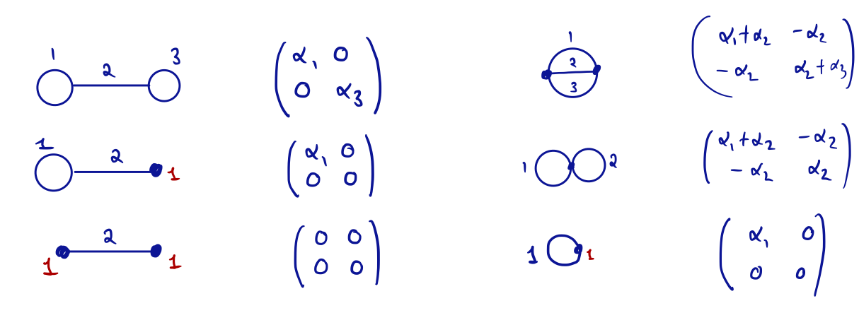
Figure 10. The graph Laplacians of the stable graphs of genus 2

Example 12.1.

Consider the sunrise diagram (figure 10, top right), with edges oriented to the right, and let $c_{1}=e_{1}-e_{2}$, $c_{2}=e_{2}-e_{3}$ denote cycles in $\mathbb{Z}^{E_{G}}$ whose image in $H_{1}(G;\mathbb{Z})$ is a basis. The graph Laplacian matrix with respect to this basis is

$$\Lambda_{G}=\begin{pmatrix}x_{1}+x_{2}&-x_{2}\\ -x_{2}&x_{2}+x_{3}\end{pmatrix}$$

with determinant $\Psi_{G}=x_{1}x_{2}+x_{1}x_{3}+x_{2}x_{3}$. The vanishing of the matrix $\Lambda_{G}$ implies that $x_{1}=x_{2}=x_{3}=0$. The Laplacians of the remaining stable graphs of genus 2 are depicted in the same figure. The tropical Torelli map is not injective on the dumbbell graph (top left), and is even identically zero on the graph depicted in the bottom left. Thus the tropical Torelli map collapses the dumbbell cell into the boundary of the image of the sunrise cell.

Let $G$ be a connected graph. The Laplacian $\Lambda_{G}$ defines a linear map

(12.3) $$\lambda_{G}:\mathbb{Q}^{E_{G}}\longrightarrow\mathcal{Q}(H_{1}(G;\mathbb{Q}))$$

which is not injective in general, as the previous example shows. When this is the case, the tropical Torelli map does not extend to a morphism in the category $\mathrm{PLC}_{\mathbb{Q}}$ because it sends boundaries of polyhedral cones into the interiors of other polyhedral cones.

Proposition 12.2.

The linear map (12.3) is injective if and only if $G$ is 3-edge connected (the removal of any edge of $G$ is connected and bridgeless).

Proof.

Suppose that $G$ is 3-edge connected. Let $e\in E_{G}$ be any edge of $e$ which is not a self-edge. The graph $G\backslash e$ is 2-edge connected. By Menger’s theorem there exist two edge-disjoint paths $p_{1},p_{2}$ between the endpoints of $e$ which lie in $G\backslash e$. It follows that, by choosing an orientation on the edges of $G$ and adjoining the edge $e$ to the paths $p_{1},p_{2}$, we may find two cycles $c_{1},c_{2}\in\mathbb{Z}^{E_{G}}$ which are independent homology classes in $H_{1}(G;\mathbb{Z})$, and only overlap in the single edge $e$. We may complete these to a family of cycles $c_{1},c_{2},\ldots,c_{h}$ which represent a basis of $H_{1}(G;\mathbb{Z})$. It follows from the definition of $\Lambda_{G}$ that the entry $(\Lambda_{G})_{1,2}=\pm x_{e}$. where the sign depends on the choice of orientation of edges, and is immaterial. Consequently, the kernel of $\Lambda_{G}$ is contained in the subspace $x_{e}=0$ of $\mathbb{Q}^{E_{G}}$. Now suppose that $e$ is a self-edge. We may choose the first cycle $c_{1}$ in a choice of representatives $c_{1},\ldots,c_{h}$ for $H_{1}(G;\mathbb{Z})$ to consist of the single edge $e$. In this case, $(\Lambda_{G})_{1,1}=\pm x_{e}$ and again we conclude that the kernel of (12.3) is contained in $x_{e}=0$ for all edges $e\in E_{G}$. Hence $\lambda_{G}$ is injective.

Conversely, if $G$ is not $3$-edge connected, there exist distinct edges $e_{1},e_{2}\in E_{G}$ such that $G^{\prime}=G\backslash\{e_{1},e_{2}\}$ is disconnected, and $G/G^{\prime}$ is a bubble graph with two vertices, two edges and a single loop. Its Laplacian is represented by the $1\times 1$ matrix with a single entry $x_{e_{1}}+x_{e_{2}}$. It follows that $\lambda_{G/G^{\prime}}$, and a fortiori $\lambda_{G}$, are not injective since the linear subspace of $\mathbb{Q}^{E_{G}}$ given by $x_{e_{1}}=-x_{e_{2}}$ and all remaining $x_{e}=0$, is contained in their kernel. ∎

The answer to a more precise question, namely when two tropical curves have equivalent Laplacians, is provided in [CV10]. Note that for any bridge $e\in E_{G}$, the variable $x_{e}$ does not appear at all in the Laplacian $\Lambda_{G}$ and one always has $\mathbb{Q}e\subset\ker(\lambda_{G})$.

12.2. Reduced moduli space of tropical curves

The set of $3$-edge connected weighted graphs is stable under edge contractions.

Definition 12.3.

Let $I_{g}^{\mathrm{red}}$ be the full subcategory of $I_{g}$ (definition 6.3) whose objects are isomorphism classes of weighted connected graphs with edge-connectivity three. Let

$$L\mathcal{M}_{g}^{\mathrm{red},\mathrm{trop}}:(I_{g}^{\mathrm{red}})^{\mathrm{opp}}\longrightarrow\mathrm{PLC}_{\mathbb{Q}}$$

denote the restriction of the functor $L\mathcal{M}_{g}^{\mathrm{trop}}$ to $(I_{g}^{\mathrm{red}})^{\mathrm{opp}}$. Similarly, let

$$\mathcal{X}^{\mathrm{red}}:(I_{g}^{\mathrm{red}})^{\mathrm{opp}}\longrightarrow\mathrm{Sch}_{\mathbb{Q}}$$

denote the restriction of the graph locus functor to $(I_{g}^{\mathrm{red}})^{\mathrm{opp}}$.

There is a natural map $L\mathcal{M}_{g}^{\mathrm{red},\mathrm{trop}}\rightarrow L\mathcal{M}_{g}^{\mathrm{trop}}$ and an inclusion $\left|L\mathcal{M}_{g}^{\mathrm{red},\mathrm{trop}}\right|\ \hookrightarrow\ \left|L\mathcal{M}_{g}^{\mathrm{trop}}\right|$. In genus 2, for example, the reduced moduli space of tropical curves has only one top-dimensional cell, which is indexed by the sunrise graph (figure 10).

12.3. The projective tropical Torelli map

Let $G$ be a 3-edge connected weighted graph. By proposition 12.2, $\lambda_{G}$ is injective and its projectivisation defines a linear morphism:

(12.4) $$\mathbb{P}^{E_{G}} \overset{[\lambda_{G}]}{\longrightarrow} \mathbb{P}(\mathcal{Q}(H_{1}(G;\mathbb{Q}))$$

$$(\alpha_{e})_{e\in E_{G}} \mapsto \left[\sum_{e}\alpha_{e}Q_{e}\right]\ ,$$

where $Q_{e}$ is the quadratic form $Q_{e}(e_{1},e_{2})=\delta_{e,e_{1}}\delta_{e,e_{2}}$. A key theorem [AB12, Defn. 3.4 and Theorem 6.7], generalised to regular matroids in [MV12, Theorem 4.2.1], states that for any such $G$, there exists a quadratic form $Q_{G}$ whose minimal vectors are exactly the set of $Q_{e}$, for $e\in E_{G}$. Thus, for every 3-edge connected graph $G$ of weight zero, the map $[\lambda_{G}]:\sigma_{G}\cong\sigma_{Q_{G}}$ is an isomorphism. Therefore $[\lambda_{G}]$ defines a morphism

(12.5) $$\mathsf{c}_{G}=(\mathbb{P}^{E_{G}},L_{G},\sigma_{G})\quad\longrightarrow\quad\mathsf{c}_{Q_{G}}=(\mathbb{P}^{Q_{G}},L_{\sigma_{Q_{G}}},\sigma_{Q_{G}})$$

in the category $\mathrm{PLC}_{\mathbb{Q}}$. The following proposition is a paraphrase of the results [BMV11] in the category of stacky fans, transposed to setting of polyhedral linear complexes.

Proposition 12.4.

There is a canonical morphism of $\mathrm{PLC}_{\mathbb{Q}}$-complexes:

(12.6) $$\lambda:L\mathcal{M}^{\mathrm{red},\mathrm{trop}}_{g}\rightarrow L\mathcal{A}^{\mathrm{trop}}_{g}$$

which maps the subscheme $\mathcal{X}^{\mathrm{red}}$ to $\mathrm{Det}$. Its topological incarnation

$$\left|L\mathcal{M}^{\mathrm{red},\mathrm{trop}}_{g}\right|\longrightarrow\left|L\mathcal{A}^{\mathrm{trop}}_{g}\right|$$

is the restriction of the tropical Torelli map (12.2) to the reduced moduli space.

Proof.

By the references quoted above, there exists a functor $t_{g}:\left(I_{g}^{\mathrm{red}}\right)^{\mathrm{opp}}\longrightarrow\mathcal{D}_{g}^{\mathrm{perf}}$ which sends a $3$-edge connected graph $G$ to $[Q_{G}]$. The pair $(t_{g},[\lambda])$ defines the required morphism of $\mathrm{PLC}_{\mathbb{Q}}$-complexes, since $[\lambda]$ is functorial and defines a natural transformation. The compatibility of $\mathcal{X}^{\mathrm{red}}$ and $\mathrm{Det}$ follows since $\Psi_{G}=\det\Lambda_{G}$, and hence $[\lambda](X_{G})=\mathrm{Det}$. ∎

12.4. The blow-up of the tropical Torelli map

Proposition 12.5.

Let $G$ be a 3-edge connected graph. Then the tropical Torelli map induces a homeomorphism:

$$\lambda^{\mathcal{B}}_{G}:\sigma^{\mathcal{B}}_{G}\overset{\sim}{\longrightarrow}\sigma^{\mathcal{B}}_{Q_{G}}\ .$$

Proof.

Because $G$ is 3-edge connected, the map $\lambda_{G}$ is injective. Since $\lambda_{G}:\sigma_{G}\cong\sigma_{Q_{G}}$ is an isomorphism and since $\mathbb{P}^{Q_{G}}$ is the Zariski-closure of $\sigma_{Q_{G}}$ it follows that (12.5) is an isomorphism in $\mathrm{PLC}_{\mathbb{Q}}$. It suffices to show that for every face $\sigma_{F}$ of $\sigma_{Q_{G}}$, one has $\mathbb{P}(\mathcal{Q}(V/K_{\sigma_{F}}))(\mathbb{R})\cap\sigma_{Q_{G}}=\sigma_{\gamma}$ for some core subgraph $\gamma\subset G$. To see this, note that since $\sigma_{G}$ is a simplex, its faces $\sigma_{G}\cap L_{\gamma}\cong\sigma_{G/\gamma}$ are in one-to-one correspondence with subgraphs $\gamma\subset G$ where $L_{\gamma}$ is the coordinate hyperplane defined by the vanishing of $x_{e}$, for $e\in E_{\gamma}$. Therefore let $\gamma\subset G$ such that $\lambda:\sigma_{G/\gamma}\cong\sigma_{F}$. We first show that $K_{\sigma_{G/\gamma}}=H_{1}(\gamma;\mathbb{Q})$. For this, choose an isomorphism $H_{1}(G;\mathbb{Q})\cong H_{1}(\gamma;\mathbb{Q})\oplus H_{1}(G/\gamma;\mathbb{Q})$. The restriction of the graph Laplacian $\Lambda_{G}$ to $L_{\gamma}$ takes the block matrix form

$$\Lambda_{G}\Big{|}_{L_{\gamma}}=\begin{pmatrix}0&0\\ 0&\Lambda_{G/\gamma}\end{pmatrix}\ .$$

Since $\det(\Lambda_{G/\gamma})=\Psi_{G/\gamma}$ is positive on $\sigma$, the kernel of this quadratic form is precisely $H_{1}(\gamma;\mathbb{Q})$ and hence $K_{\sigma_{G/\gamma}}=H_{1}(\gamma;\mathbb{Q})$. Let $\gamma^{\mathrm{core}}$ denote the largest core subgraph of $\gamma$. Since $H_{1}(\gamma;\mathbb{Q})=H_{1}(\gamma^{\mathrm{core}};\mathbb{Q})$, we deduce that $\mathbb{P}(\mathcal{Q}(V/H_{1}(\gamma;\mathbb{Q}))(\mathbb{R})\cap\sigma_{G}$ contains $\sigma_{\gamma^{\mathrm{core}}}$. To show the reverse inclusion, note that the restriction of $\Lambda_{G}$ to $H^{1}(\gamma;\mathbb{Q})$ is $\Lambda_{\gamma}$, whose determinant is $\Psi_{\gamma}=\Psi_{\gamma^{\mathrm{core}}}$. Thus the intersection of $\sigma$ with the vanishing locus of $\Lambda_{\gamma}$ is contained in the locus of $\sigma$ such that $\Psi_{\gamma^{\mathrm{core}}}=0.$ But this implies that $x_{e}=0$ for all $e\in E_{\gamma^{\mathrm{core}}}$ by the positivity of core graph polynomials. Hence $\mathbb{P}(\mathcal{Q}(V/H_{1}(\gamma;\mathbb{Q}))(\mathbb{R})\cap\sigma_{G}=\sigma_{\gamma^{\mathrm{core}}}$. ∎

Define $L\mathcal{M}^{\mathrm{red},\mathcal{B}}_{g}$ to be the restriction of the functor $L\mathcal{M}^{\mathrm{trop},\mathcal{B}}_{g}$ to the (opposite of the) subcategory $I_{g}^{\mathrm{red},\mathcal{B}}$ of $I_{g}^{\mathcal{B}}$ generated by the images of three-edge connected graphs under admissible edge contractions and refinements (definition 7.4).

Theorem 12.6.

The tropical Torelli map induces a continuous map

$$\lambda^{\mathcal{B}}:|L\mathcal{M}^{\mathrm{red},\mathcal{B}}_{g}|\longrightarrow|L\mathcal{A}^{\mathrm{trop},\mathcal{B}}_{g}|$$

which maps $|\partial L\mathcal{M}^{\mathrm{red},\mathcal{B}}_{g}|$ to $|\partial L\mathcal{A}^{\mathrm{trop},\mathcal{B}}_{g}|$ and is compatible, via the canonical blow-down maps with the Torelli map (12.6).

Proof.

This follows from propositions 12.5 and (12.6), which makes essential use of the theorem of [AB12] on the existence and functoriality of $[Q_{G}]$, for $G$ a graph. ∎

13. Canonical bi-invariant forms and their integrals

13.1. Canonical forms

Employing the same notation as in [Bro21], we define

(13.1) $$\Omega_{\mathrm{can}}=\bigwedge\bigoplus_{k\geq 1}\mathbb{Q}\,\omega^{4k+1}$$

to be the graded-commutative Hopf algebra generated by elements $\omega^{4k+1}$ in degree $4k+1$, where the coproduct $\Delta^{\mathrm{can}}:\Omega^{\mathrm{can}}\rightarrow\Omega^{\mathrm{can}}\otimes_{\mathbb{Q}}\Omega^{\mathrm{can}}$ has the property that the $\omega^{4k+1}$ are primitive, i.e., $\Delta^{\mathrm{can}}(\omega^{4k+1})=\omega^{4k+1}\otimes 1+1\otimes\omega^{4k+1}$.

Let $R=\bigoplus_{n\geq 0}R^{n}$ be a differential graded algebra and let $X\in\mathrm{GL}_{g}(R^{0})$ be an invertible $g\times g$ symmetric matrix. We denote by

$$\omega_{X}^{4k+1}=\mathrm{tr}\left((X^{-1}dX)^{4k+1}\right)\quad\in\quad R^{4k+1}\ .$$

More generally, any $\omega\in\Omega_{\mathrm{can}}$ is a polynomial in the $\omega^{4k+1}$. We write $\omega_{X}$ for the corresponding polynomial in the $\omega_{X}^{4k+1}$. One can show that $\omega_{X}$ are:

1. Closed: $d\omega_{X}=0$ for any $X$ as above.

2. Bi-invariant: $\omega_{AXB}=\omega_{X}$ for all $A,B\in\mathrm{GL}_{g}(R^{0})$ such that $dA=dB=0$.

3. Additive: if we write $\Delta^{\mathrm{can}}\omega=\sum\omega^{\prime}\otimes\omega^{\prime\prime}$ and $X_{1},X_{2}\in\mathrm{GL}_{g}(R^{0})$, then

   $$\omega_{X_{1}\oplus X_{2}}=\sum\omega^{\prime}_{X_{1}}\wedge\omega^{\prime\prime}_{X_{2}}\ .$$

4. Projective: $\omega_{\lambda X}=\omega_{X}$ for all $\lambda\in(R^{0})^{\times}$,

5. Vanish in low rank: $\omega^{4k+1}_{X}=0$ if $4k+1>2g.$

See [Bro21] for proofs. Borel showed in [Bor74] that $\Omega_{\mathrm{can}}\overset{\sim}{\rightarrow}\varprojlim H^{\bullet}(\mathrm{GL}_{g}(\mathbb{Z});\mathbb{R})$.

13.2. Forms of ‘compact type’

Let $g>1$ be odd. By the vanishing property (5), only a finite subspace of $\Omega_{\mathrm{can}}$ is non-zero on $g\times g$ symmetric matrices.

Definition 13.1.

Let $\Omega(g)\subset\Omega_{\mathrm{can}}$ denote the graded exterior algebra generated by $1$, $\omega^{5}$ , …, $\omega^{2g-1}$. It is naturally a quotient of $\Omega_{\mathrm{can}}$ via the map $\Omega_{\mathrm{can}}\rightarrow\Omega(g)$ which sends $\omega^{4k+1}$ to zero for all $2k>g$. We shall call a form simple if it is a monomial in the generators of $\Omega(g)$, i.e., a product of primitive elements. An element of $\Omega(g)$ is a finite linear combination of simple forms. Call a form $\omega\in\Omega(g)$ of compact type relative to $g$ if it is divisible by $\omega^{2g-1}$

(13.2) $$\omega=\eta\wedge\omega^{2g-1}\quad\hbox{ for some }\ \eta\in\Omega(g)\ .$$

Otherwise, a simple form $\omega$ will be called of non-compact type. Denote the space spanned by forms of compact (resp. non-compact) type by $\Omega_{c}(g)$ (resp. $\Omega_{nc}(g)$). We have

$$\Omega(g)=\Omega_{c}(g)\oplus\Omega_{nc}(g)$$

The subspace $\Omega_{c}(g)\subset\Omega(g)$ is an ideal.

Consider the volume form

(13.3) $$\mathrm{vol}_{g}=\omega^{5}\wedge\ldots\wedge\omega^{2g-1}\quad\in\quad\Omega_{c}(g)$$

which is of degree $d_{g}-1$, where $d_{g}=\frac{g(g+1)}{2}$. It is simple, and of compact type.

Definition 13.2.

Let $\omega\in\Omega(g)$ be simple. There is a unique $\star\omega\in\Omega(g)$ such that

$$\omega\wedge\star\omega=\mathrm{vol}_{g}\ .$$

The map $\star$ extends by linearity to an endomorphism (the Hodge star operator) on $\Omega(g)$ which interchanges the subspaces of forms of compact and non-compact types:

$$\star:\Omega_{c}(g)\overset{\sim}{\longrightarrow}\Omega_{nc}(g)\ .$$

It is an involution up to sign: $\star\star\omega=\pm\omega$.

Example 13.3.

Let $g=7$. Then $\mathrm{vol}_{7}=\omega^{5}\wedge\omega^{9}\wedge\omega^{13}$. The following table lists the simple elements in $\Omega_{nc}(7)$, and below them, their images in $\Omega_{c}(7)$ under the map $\star$:

$$\begin{array}[]{cccc}\quad 1&\quad\omega^{5}&\quad\omega^{9}&\quad\omega^{5}\wedge\omega^{9}\\ \quad\downarrow&\quad\downarrow&\quad\downarrow&\quad\downarrow\\ \omega^{5}\wedge\omega^{9}\wedge\omega^{13}&\quad\omega^{9}\wedge\omega^{13}&\quad-\,\omega^{5}\wedge\omega^{13}&\quad\omega^{13}\end{array}$$

13.3. Canonical forms on $L\mathcal{M}_{g}^{\mathrm{trop}}$ and $L\mathcal{A}_{g}^{\mathrm{trop}}$.

Lemma 13.4.

Let $\omega\in\Omega_{\mathrm{can}}$ be a canonical form of degree $d$, and let $V$ be a vector space over $k\subset\mathbb{R}$. Then $\omega$ defines a closed projective differential form

$$\omega\quad\in\quad\Omega^{d}(\mathbb{P}(\mathcal{Q}(V))\backslash\mathrm{Det})$$

which is invariant under the action of $\mathrm{GL}(V)$.

Proof.

The projectivity follows from §13.1 (4), the invariance from (2). ∎

Proposition 13.5.

A canonical form $\omega\in\Omega^{d}(g)$ defines an algebraic differential form (§2.4):

(13.4) $$\omega\quad\in\quad\Omega^{d}(L\mathcal{A}_{g}^{\mathrm{trop}}\backslash\mathrm{Det})$$

It restricts to a smooth differential form, also denoted by $\omega$, on

$$\omega\quad\in\quad\mathcal{A}^{d}\left(\left|L\mathcal{A}^{\circ,\mathrm{trop}}_{g}\right|\right)=\mathcal{A}^{d}\left(L\mathcal{P}_{g}/\mathrm{GL}_{g}(\mathbb{Z})\right)$$

Proof.

By definition 2.9 a differential form must verify the compatibility relations (2.8). A canonical form $\omega$ satisfies the compatibilities for the two types of morphisms in the category $\mathcal{D}_{g}^{\mathrm{perf}}$ of definition 10.5: for face morphisms, the compatibility is automatic, and for isomorphisms, this follows from the bi-invariance §13.1 (2). The fact that $\omega$ only has poles along the determinant locus follows immediately from its definition since for any square matrix $X$, the one-form $X^{-1}dX$ is regular outside the locus $\det(X)=0$. ∎

In [Bro21], we studied the canonical forms $\omega_{G}=\omega_{\Lambda_{G}}$ on the polyhedral linear configuration associated to a graph $G$. A result in that paper may be paraphrased as follows.

Proposition 13.6.

A form $\omega\in\Omega^{d}(g)$ defines an algebraic form $\omega\in\Omega^{d}(L\mathcal{M}_{g}^{\mathrm{trop}}\backslash\mathcal{X})$. It restricts to a smooth differential form, also denoted by $\omega$, on

$$\omega\quad\in\quad\mathcal{A}^{d}\left(\left|L\mathcal{M}^{\mathrm{trop}}_{g}\right|\backslash\left|\partial L\mathcal{M}^{\mathrm{trop}}_{g}\right|\right)\ .$$

The restriction of $\omega$ to the reduced moduli space $L\mathcal{M}_{g}^{\mathrm{red},\mathrm{trop}}$ is the pull-back $\lambda_{G}^{*}\omega$ of the corresponding canonical forms (13.4) on $L\mathcal{A}_{g}^{\mathrm{trop}}$ by the tropical Torelli map.

13.4. Behaviour at infinity

A key property of canonical forms is their behaviour on blow-ups and in particular, a factorisation property at infinity.

Proposition 13.7.

Let $0\leq K\subset V$ be a subspace and let $\pi:\mathbb{P}\rightarrow\mathbb{P}(\mathcal{Q}(V))$ denote the blow-up along $\mathbb{P}(\mathcal{Q}(V/K))$. Let $\omega\in\Omega^{d}_{\mathrm{can}}$. Denote its coproduct by

$$\Delta^{\mathrm{can}}\omega=\sum_{i}\omega_{i}^{\prime}\otimes\omega_{i}^{\prime\prime}\ .$$

The pull-back $\pi^{*}\omega$ to $\mathbb{P}$ has no poles along the exceptional divisor, and hence defines a regular differential form on the complement of the strict transform $\widetilde{\mathrm{Det}}$ of the determinant locus:

$$\pi^{*}(\omega)\quad\in\quad\Omega^{d}\left(\mathbb{P}\,\setminus\,\widetilde{\mathrm{Det}}\right)\ .$$

Its restriction to the exceptional divisor $\mathcal{E}$, which we recall by proposition 9.10 is canonically isomorphic to the product $\mathcal{E}=\mathbb{P}\left(\mathcal{Q}(V/K)\right)\times\mathbb{P}\left(\mathcal{Q}(V)/\mathcal{Q}(V/K)\right)$, satisfies

(13.5) $$\pi^{*}(\omega)\big{|}_{\mathcal{E}}=\sum_{i}\omega_{i}^{\prime}\wedge\pi_{K}^{*}(\omega_{i}^{\prime\prime})$$

where $\omega_{i}^{\prime}\in\Omega^{\bullet}\left(\mathbb{P}(\mathcal{Q}(V/K))\backslash\mathrm{Det}_{V/K}\right)$, $\omega_{i}^{\prime\prime}\in\Omega^{\bullet}\left(\mathbb{P}\left(\mathcal{Q}(K)\right)\backslash\mathrm{Det}_{K}\right)$, and $\pi_{K}$ is the map (9.7).

Proof.

The proof is almost identical to that of theorem 7.4 in [Bro21] to which we refer for further details. The key point is to write formula (9.11) in the form:

$$s_{K}^{*}Q=\begin{pmatrix}zQ_{K}&zP\\ zP^{T}&Q_{C}\end{pmatrix}=\Lambda U\quad\hbox{ where we set }\quad\Lambda=\begin{pmatrix}zQ_{K}&0\\ 0&Q_{C}\end{pmatrix}\ ,$$

and where

$$U=\Lambda^{-1}s_{K}^{*}Q\equiv\begin{pmatrix}1&Q_{K}^{-1}P\\ 0&1\end{pmatrix}\pmod{z}\ .$$

For simplicity, assume that $\omega=\omega^{4k+1}$ is primitive. Then

$$\omega^{4k+1}_{\Lambda U}=\mathrm{tr}\left((U^{-1}\Lambda^{-1}(d\Lambda)U+U^{-1}dU)^{4k+1}\right)=\mathrm{tr}\left(\left(\Lambda^{-1}d\Lambda+dU.U^{-1}\right)^{4k+1}\right)$$

The argument follows exactly as in theorem 7.4 of loc. cit. to conclude that

$$\omega_{s_{K}^{*}Q}\Big{|}_{z=0}=\omega^{4k+1}_{Q_{C}}+\omega^{4k+1}_{Q_{K}}$$

and hence $\pi^{*}(\omega)\big{|}_{\mathcal{E}}=\omega^{4k+1}_{Q_{C}}\wedge 1+1\wedge\omega^{4k+1}_{Q_{K}}$. The case when $\omega$ is a simple form follows by multiplying primitive forms together; the general case follows by linearity. ∎

Remark 13.8.

This implies that the restriction of $\pi^{*}(\omega)$ to the exceptional divisor is actually just the pre-image of canonical forms under the collapsing map §9.3 of the normal bundle.

It may often happen that the restriction $\pi^{*}(\omega)$ to the exceptional divisor $\mathcal{E}$ vanishes. There is one important situation in which this always occurs.

Corollary 13.9.

Let $\omega\in\Omega^{d}_{c}(g)$ be of compact type, where $g=\dim(V)>1$ is odd. Then, in the situation of proposition 13.7, $\pi^{*}\omega$ vanishes along the exceptional divisor $\mathcal{E}$.

Proof.

We may assume that $\omega$ is simple. Since $\omega$ is of compact type, it follows that in the expression $\Delta^{\mathrm{can}}\omega=\sum_{i}\omega_{i}^{\prime}\otimes\omega_{i}^{\prime\prime}$ either $\omega_{i}^{\prime}$ or $\omega_{i}^{\prime\prime}$ is of compact type for each $i$, since one of these two forms must be divisible by $\omega^{2g-1}$. Since $K\neq 0$, the vanishing property §13.1 (5) implies that either $(\omega_{i}^{\prime})_{Q_{K}}=0$ or $(\omega_{i}^{\prime\prime})_{Q_{C}}=0$ for every $i$, since both $Q_{K}$ and $Q_{C}$ have strictly smaller rank $<g$. It follows from the formula (13.5) that $\pi^{*}(\omega)$ vanishes along $\mathcal{E}$. ∎

The essential part of the proof is the fact that $\Omega_{c}(g)$ is a Hopf ideal in $\Omega(g)$:

$$\Delta^{\mathrm{can}}(\Omega_{c}(g))\ \subset\ \left(\Omega_{c}(g)\otimes_{\mathbb{Q}}\Omega_{nc}(g)\right)+\left(\Omega_{nc}(g)\otimes_{\mathbb{Q}}\Omega_{c}(g)\right)\ .$$

13.5. Canonical forms on $L\mathcal{A}_{g}^{\mathrm{trop},\mathcal{B}}$ and $L\mathcal{M}_{g}^{\mathrm{trop},\mathcal{B}}$

Theorem 13.10.

Let $\omega\in\Omega^{d}_{\mathrm{can}}$. It defines an algebraic differential form

(13.6) $$\widetilde{\omega}\in\Omega^{d}\left(L\mathcal{A}_{g}^{\mathrm{trop},\mathcal{B}}\backslash\widetilde{\mathrm{Det}}\right)$$

which restricts to a smooth form, also denoted by the same notation,

(13.7) $$\widetilde{\omega}\in\mathcal{A}^{d}\left(\left|L\mathcal{A}_{g}^{\mathrm{trop},\mathcal{B}}\right|\right)$$

on the topological realisation. In the case when $g>1$ is odd and $\omega\in\Omega^{d}_{c}(g)$ is of compact type, then the restriction of (13.6) to the boundary $\partial L\mathcal{A}_{g}^{\mathrm{trop},\mathcal{B}}\ \backslash\ (\partial L\mathcal{A}_{g}^{\mathrm{trop},\mathcal{B}}\cap\widetilde{\mathrm{Det}})$ vanishes.

Proof.

Let $Q$ be a positive definite quadratic form such that $\sigma_{Q}>0$. Let $\widetilde{\omega}=\pi^{*}\omega$ denote the pull-back of the form $\omega$ along the iterated blow-up $\pi:P^{\mathcal{B}_{Q}}\rightarrow\mathbb{P}^{Q}.$ By repeated application of proposition 13.7 for each blow-up in the formation of $P^{\mathcal{B}_{Q}}$, we deduce that $\widetilde{\omega}$ is a meromorphic differential form with no poles along the exceptional divisor. It follows that $\widetilde{\omega}\in\Omega^{d}(P^{\mathcal{B}_{Q}}\ \backslash\ \widetilde{\mathrm{Det}})$. By restricting it to faces, we obtain a family of forms in $\Omega^{d}((\mathsf{S}L\mathcal{A}^{\mathrm{trop},\mathcal{B}}_{g}\backslash\widetilde{\mathrm{Det}})(x))$ for every object $x$ of $\mathcal{D}_{g}^{\mathrm{perf}}$. By the universal property of strict transforms (proposition 5.2 (i)) and the fact that restriction of differential forms is compatible with pull-back along blow-ups, the compatibility conditions (2.8) for $\widetilde{\omega}$ follow from those of $\omega$, established in proposition 13.5. This is because the objects in a face diagram (10.5) are the blow-ups of a face map in $\mathcal{D}_{g}^{\mathrm{perf}}$, and the form $\widetilde{\omega}$ on each component is the pull-back of $\omega$ along a suitable blow-up.

The statement (13.7) is a consequence of the fact that $\left|L\mathcal{A}_{g}^{\mathrm{trop},\mathcal{B}}\right|$ does not meet the strict transform of the determinant locus (theorem 11.3). When $\omega$ is of compact type, $\widetilde{\omega}$ vanishes along exceptional divisors by the second part of proposition 13.7. ∎

The following statement for $L\mathcal{M}_{G}^{\mathrm{trop},\mathcal{B}}$ may be proved using [Bro21].

Theorem 13.11.

Let $\omega\in\Omega^{d}_{\mathrm{can}}$. It defines both a holomorphic differential form, and a smooth form on which we may denote by:

(13.8) $$\widetilde{\omega}\in\Omega^{d}\left(L\mathcal{M}_{g}^{\mathrm{trop},\mathcal{B}}\backslash\widetilde{\mathcal{X}}\right)\qquad\hbox{resp. }\qquad\widetilde{\omega}\in\mathcal{A}^{d}\left(\left|L\mathcal{M}_{g}^{\mathrm{trop},\mathcal{B}}\right|\right)\ .$$

Note that in the case of $L\mathcal{M}_{g}^{\mathrm{trop},\mathcal{B}}$ the existence of the dual graph Laplacian implies that most forms of compact type actually vanish (see [Bro21], Lemma 8.4) except for the primitive ones. See the discussion in §14.6.

13.6. Integrals of canonical forms

Canonical integrals define new invariants associated to the minimal vectors of quadratic forms.

Corollary 13.12.

Let $Q$ be a positive definite quadratic form such that $\sigma_{Q}$ is strictly positive. Then for any canonical form $\omega\in\Omega^{d}_{\mathrm{can}}$ where $d=\dim\sigma_{Q}$, the integral

$$I_{Q}(\omega)=\int_{\sigma_{Q}}\omega$$

is finite. In the case where $Q=Q_{G}$ is the image of a graph, the integral $I_{Q_{G}}(\omega)$ reduces to the canonical integrals $I_{G}(\omega)$ studied in [Bro21].

Proof.

By passing to the blow-up $P^{\mathcal{B}_{Q}}\rightarrow\mathbb{P}^{Q}$, we may write

$$I_{Q}(\omega)=\int_{\sigma^{\mathcal{B}}_{Q}}\widetilde{\omega}$$

since $\overset{\circ}{\sigma}_{Q}$ is contained in $\sigma^{\mathcal{B}}_{Q}$, and has complement of Lebesgue measure zero. By theorem 11.3, $\widetilde{\omega}$ has no poles along the compact region $\sigma^{\mathcal{B}}_{Q}$ and therefore the integral is finite. ∎

These integrals satisfy many interesting relations. The analogous relations for graphs were studied in [Bro21] and related to the ‘waterfall’ spectral sequence of [KWv17].

Theorem 13.13.

(Stokes relation). Let $Q$ be a positive definite quadratic form such that $\sigma_{Q}>0$, and let $\omega\in\Omega_{\mathrm{can}}$ have degree $\dim\sigma_{Q}-1$. Let $\Delta^{\mathrm{can}}\omega=\sum_{i}\omega^{\prime}_{i}\otimes\omega^{\prime\prime}_{i}$. Then

(13.9) $$0=\sum_{Q^{\prime}}\int_{\sigma_{Q^{\prime}}}\omega+\sum_{i}\sum_{F}\int_{\sigma_{F}}\omega^{\prime}_{i}\int_{\sigma_{Q}/\sigma_{F}}\pi^{*}_{K_{\sigma_{F}}}(\omega^{\prime\prime}_{i})$$

where $Q^{\prime}\leq Q$ denote the facets of $\sigma_{Q}$ which are strictly positive (not contained in $\mathrm{Det}(\mathbb{R})$), and $\sigma_{F}\times\sigma_{Q}/\sigma_{F}$ denote the set of facets of its blow-up $\sigma^{\mathcal{B}_{Q}}_{Q}$ which are at infinity (in other words, $\sigma_{F}$ is an essential face of $\sigma_{Q}$ at infinity, and $\sigma_{Q}/\sigma_{F}$ is defined in (9.8)). The map $\pi_{K_{\sigma_{F}}}$ is defined in lemma 9.7.

Proof.

This follows from an application of Stokes’ formula:

$$0=\int_{\sigma^{\mathcal{B}}_{Q}}d\widetilde{\omega}=\int_{\partial\sigma^{\mathcal{B}}_{Q}}\widetilde{\omega}\ ,$$

the description of the boundary facets of $\sigma^{\mathcal{B}}_{Q}$, and the factorisation formula (13.5). ∎

13.7. Compactly-supported representatives

Every form of compact type has a representative which vanishes identically in a neighbourhood of the boundary.

Corollary 13.14.

Let $g>1$ be odd. The cohomology class of the differential form $\omega^{2g-1}$ in $H_{dR}^{2g-1}(\left|L\mathcal{A}_{g}^{\mathrm{trop},\mathcal{B}}\right|,\left|\partial L\mathcal{A}_{g}^{\mathrm{trop},\mathcal{B}}\right|)$ has a compactly supported representive

$$[\omega^{2g-1}_{c}]\ \in\ H_{dR,c}^{2g-1}(\left|L\mathcal{A}_{g}^{\circ,\mathrm{trop}}\right|)\ .$$

Having chosen $\omega^{2g-1}_{c}$, any other form $\omega=\omega^{2g-1}\wedge\eta\in\Omega_{c}(g)$ of compact type has a canonical compactly supported representative $\omega_{c}=\omega^{2g-1}_{c}\wedge\eta$.

Proof.

By (3.9), and (11.7) we have $H^{\bullet}_{dR,c}(\left|L\mathcal{A}_{g}^{\circ,\mathrm{trop}}\right|)\cong H_{dR}^{\bullet}(\left|L\mathcal{A}_{g}^{\mathrm{trop},\mathcal{B}}\right|,\left|\partial L\mathcal{A}_{g}^{\mathrm{trop},\mathcal{B}}\right|)$. The form $\omega^{2g-1}$, being of compact type, vanishes on $\left|\partial L\mathcal{A}_{g}^{\mathrm{trop},\mathcal{B}}\right|$ by theorem 13.10 and therefore defines a class in the latter cohomology group. ∎

The fact that $\omega^{2g-1}$ has a compactly supported representative on $L\mathcal{P}_{g}/\mathrm{GL}_{g}(\mathbb{Z})$ was announced in [Lee78]. Since one also has $\left|L\mathcal{A}_{g}^{\circ,\mathrm{trop}}\right|=\left|L\mathcal{A}_{g}^{\mathrm{trop}}\right|\setminus\left|\partial L\mathcal{A}_{g}^{\mathrm{trop}}\right|$, the blow-down map $\pi:|L\mathcal{A}_{g}^{\mathrm{trop},\mathcal{B}}|\rightarrow\left|L\mathcal{A}_{g}^{\mathrm{trop}}\right|$ induces an isomorphism:

$$\pi^{*}:H_{dR}^{\bullet}(\left|L\mathcal{A}_{g}^{\mathrm{trop}}\right|,\left|\partial L\mathcal{A}_{g}^{\mathrm{trop}}\right|)\overset{\sim}{\longrightarrow}H_{dR}^{\bullet}(\left|L\mathcal{A}_{g}^{\mathrm{trop},\mathcal{B}}\right|,\left|\partial L\mathcal{A}_{g}^{\mathrm{trop},\mathcal{B}}\right|)$$

since both sides may be identified with the compactly supported cohomology of the interior $\left|L\mathcal{A}_{g}^{\circ,\mathrm{trop}}\right|$. In particular, any compactly supported form $\omega_{c}$ as in the corollary may be viewed as a closed differential form on $\left|L\mathcal{A}_{g}^{\mathrm{trop}}\right|$. Its cohomology class

(13.10) $$[\omega_{c}]\in H_{dR}^{\bullet}(\left|L\mathcal{A}_{g}^{\mathrm{trop}}\right|)$$

does not depend on the choice of representative for $\omega_{c}^{2g-1}$ since it is the image of $(\pi^{*})^{-1}[\widetilde{\omega}]$ under the natural map $H_{dR}^{\bullet}(\left|L\mathcal{A}_{g}^{\mathrm{trop}}\right|,\left|\partial L\mathcal{A}_{g}^{\mathrm{trop}}\right|)\rightarrow H_{dR}^{\bullet}(\left|L\mathcal{A}_{g}^{\mathrm{trop}}\right|).$

14. Cohomology classes in $\left|L\mathcal{A}_{g}^{\mathrm{trop}}\right|$.

In this section we prove the theorems announced in the introduction.

14.1. Canonical Classes in $\left|L\mathcal{A}_{g}^{\mathrm{trop}}\right|$

Let $g>1$ be odd and $\ell_{g}=\frac{g(g+1)}{2}-1$.

Lemma 14.1.

The form $\mathrm{vol}_{g}$ (13.3) defines a non-trivial relative cohomology class

$$0\neq[\mathrm{vol}_{g}]\ \in\ H_{dR}^{\ell_{g}}\left(|L\mathcal{A}_{g}^{\mathrm{trop},\mathcal{B}}|,|\partial L\mathcal{A}_{g}^{\mathrm{trop},\mathcal{B}}|\right).$$

Proof.

Since $g$ is odd, the space $L\mathcal{P}_{g}/\mathrm{GL}_{g}(\mathbb{Z})$ is orientable and has a relative fundamental class $[\mathcal{F}^{\mathrm{lf}}_{g}]\in H^{\mathrm{lf}}_{\ell_{g}}\left(\left|L\mathcal{A}_{g}^{\circ,\mathrm{trop}}\right|\right)$ in locally finite homology, or equivalently,

$$[\mathcal{F}^{\mathrm{lf}}_{g}]\in H_{\ell_{g}}\left(\left|L\mathcal{A}_{g}^{\mathrm{trop},\mathcal{B}}\right|,\left|\partial L\mathcal{A}_{g}^{\mathrm{trop},\mathcal{B}}\right|\right)\ .$$

A volume form $\eta_{g}$ on $L\mathcal{P}_{g}/\mathrm{GL}_{g}(\mathbb{Z})$ is defined on symmetric matrices $M=(M_{ij})_{ij}$ by

$$\eta_{g}(M)=\partial\left(\frac{1}{\det(M)^{\frac{g+1}{2}}}\bigwedge_{1\leq i\leq j\leq g}dM_{ij}\right)$$

where $\partial=\sum_{i,j}\frac{\partial}{\partial M_{ij}}$ is the Euler vector field. By the theory of invariant differential forms, there exists $\alpha\in\mathbb{Q}^{\times}$ such that $\eta_{g}=\alpha\,\mathrm{vol}_{g}=\alpha\,\omega^{5}\wedge\omega^{9}\wedge\ldots\wedge\omega^{2g-1}$. We have

$$\mathrm{vol}(L\mathcal{P}_{g}/\mathrm{GL}_{g}(\mathbb{Z}))=\int_{L\mathcal{P}_{g}/\mathrm{GL}_{g}(\mathbb{Z})}\eta_{g}=\alpha\int_{[\mathcal{F}^{\mathrm{lf}}_{g}]}\mathrm{vol}_{g}\ .$$

Since $\mathrm{vol}(L\mathcal{P}_{g}/\mathrm{GL}_{g}(\mathbb{Z}))\neq 0$ (for a more precise statement see (14.1)), we deduce that the cohomology class of $[\mathrm{vol}_{g}]$ in $H_{dR}^{\ell_{g}}\left(|L\mathcal{A}_{g}^{\mathrm{trop},\mathcal{B}}|,|\partial L\mathcal{A}_{g}^{\mathrm{trop},\mathcal{B}}|\right)$ is non-zero. ∎

Remark 14.2.

It follows from a theorem of Minkowski (see [Sie36]) that

(14.1) $$\int_{L\mathcal{P}_{g}/\mathrm{GL}_{g}(\mathbb{Z})}\eta_{g}\ \in\ \zeta(3)\zeta(5)\ldots\zeta(2g-1)\,\mathbb{Q}^{\times}\ .$$

The point is that the volume of the symmetric space $\mathrm{SL}_{g}(\mathbb{R})/\mathrm{SL}_{g}(\mathbb{Z})$ is proportional, by a rational number, to the product of consecutive zeta values $\zeta(2)\ldots\zeta(2g-1)$. One proves [Vos95] that the volume of $L\mathcal{P}_{g}/\mathrm{GL}_{g}(\mathbb{Z})$ is obtained by dividing by the volume of $\mathrm{SO}_{g}(\mathbb{R})$, which is proportional to the product of the even zeta values $\zeta(2)\ldots\zeta(2g-2)$, giving (14.1).

Theorem 14.3.

The map $\omega\mapsto[\omega_{c}]$ (13.10) induces an injective map of graded algebras

$$\Omega^{\bullet}_{c}(g)\hookrightarrow H_{dR}^{\bullet}\left(\left|L\mathcal{A}_{g}^{\mathrm{trop}}\right|\right)\ .$$

It factors through an injective map $\Omega^{\bullet}_{c}(g)\hookrightarrow H_{dR}^{\bullet}\left(\left|L\mathcal{A}_{g}^{\mathrm{trop}}\right|,\left|\partial L\mathcal{A}_{g}^{\mathrm{trop}}\right|\right)$.

Proof.

We prove a stronger result, namely that the classes $\Omega^{\bullet}_{c}(g)$ are non-zero in a larger complex of differential forms with ‘reduced’ boundary:

$$\Omega^{\bullet,\mathrm{red}}(L\mathcal{A}_{g}^{\mathrm{trop},\mathcal{B}})\quad\subset\quad\Omega^{\bullet}(L\mathcal{A}_{g}^{\mathrm{trop},\mathcal{B}}\ \setminus\ \widetilde{\mathrm{Det}})\ \oplus\ \bigoplus_{\mathcal{E}}\Omega^{\bullet}\left(\prod_{i=0}^{n}\mathbb{P}\left(\mathcal{Q}(K_{i+1}/K_{i})\backslash\mathrm{Det}_{K_{i+1}/K_{i}}\right)\right)$$

where the direct sum is over all components of the boundary $\partial L\mathcal{A}_{g}^{\mathcal{B}}$ indexed by flags (11.2). It consists of pairs $(\omega,(\eta_{\mathcal{E}})_{\mathcal{E}})$ such that the restriction of $\omega$ to a face $\mathcal{E}\cap\partial L\mathcal{A}_{g}^{\mathcal{B}}$ satisfies

(14.2) $$\omega\big{|}_{\mathcal{E}}=\pi_{\mathrm{red}}^{*}\,\eta_{\mathcal{E}}$$

where $\pi_{\mathrm{red}}$ was defined in (11.4). There is a corresponding complex $\mathcal{A}^{\bullet,\mathrm{red}}(|L\mathcal{A}_{g}^{\mathrm{trop},\mathcal{B}}|)$ of smooth differential forms defined in the same way: it consists of smooth forms $(\omega,(\eta_{\mathcal{E}})_{\mathcal{E}})$, where $\omega\in\mathcal{A}^{\bullet}(|L\mathcal{A}_{g}^{\mathrm{trop},\mathcal{B}}|)$ and $\eta_{\mathcal{E}}$ are smooth forms on a neighbourhood of $\pi_{\mathrm{red}}(|\partial L\mathcal{A}_{g}^{\mathrm{trop},\mathcal{B}}|\cap\mathcal{E}(\mathbb{R}))$ which satisfy (14.2). Let us denote its cohomology by $H^{\bullet,\mathrm{red}}(|L\mathcal{A}_{g}^{\mathrm{trop},\mathcal{B}}|)$.

Since the restriction of the blow down to the boundary $|\partial L\mathcal{A}_{g}^{\mathrm{trop},\mathcal{B}}|\rightarrow|\partial L\mathcal{A}_{g}^{\mathrm{trop}}|$ factors through $\pi_{\mathrm{red}}$ (it factors through the map which projects a product (11.3) onto its final component), it follows that the map on cohomology induced by $\pi_{\mathcal{B}}:|L\mathcal{A}_{g}^{\mathrm{trop},\mathcal{B}}|\rightarrow|L\mathcal{A}_{g}^{\mathrm{trop}}|$ factors through the reduced cohomology. More precisely there is a commuting diagram

(14.3) $$H^{\bullet}_{dR}(|L\mathcal{A}_{g}^{\mathrm{trop}}|)\longrightarrow H^{\bullet,\mathrm{red}}_{dR}(|L\mathcal{A}_{g}^{\mathrm{trop},\mathcal{B}}|)\longrightarrow H^{\bullet}_{dR}(|L\mathcal{A}_{g}^{\mathrm{trop},\mathcal{B}}|)$$

where the first map is induced by $\pi_{\mathcal{B}}^{*}$ and the second is $(\omega,\eta)\mapsto\omega$. We will show that

$$\omega\mapsto(\omega,0)\ :\ \Omega^{\bullet}(g)\longrightarrow H^{\bullet,\mathrm{red}}_{dR}(|L\mathcal{A}_{g}^{\mathrm{trop},\mathcal{B}}|)$$

is an injection. This map is well-defined by equation (13.5), which implies that the restriction of a canonical form to an exceptional divisor $\mathcal{E}$ is always of the form $\pi^{*}_{\mathrm{red}}(\eta)$.

We first show that the volume form is non-zero in $H^{\ell_{g},\mathrm{red}}(|L\mathcal{A}_{g}^{\mathrm{trop},\mathcal{B}}|)$. If $\mathrm{vol}_{g}$ were exact, there would exist forms $\alpha$ on $|L\mathcal{A}_{g}^{\mathrm{trop},\mathcal{B}}|$ and $(\beta_{\mathcal{E}})_{\mathcal{E}}$ of degree $\ell_{g}-1$ such that

(14.4) $$\mathrm{vol}_{g}=d\alpha\quad\hbox{ and }\quad\alpha\Big{|}_{\mathcal{E}(\mathbb{R})}=\pi_{\mathrm{red}}^{*}\beta\ .$$

However, since $\pi_{\mathrm{red}}$ decreases the dimension by at least $g-1$, such a form $\beta$ is necessarily zero since it has degree $>\ell_{g}-g$. Equation (14.4) then implies that $\mathrm{vol}_{g}$ is zero in relative cohomology $H^{\ell_{g}}_{dR}\left(\left|L\mathcal{A}_{g}^{\mathrm{trop},\mathcal{B}}\right|,\left|\partial L\mathcal{A}_{g}^{\mathrm{trop},\mathcal{B}}\right|\right)$ which contradicts lemma 14.1.

Now let $\omega\in\Omega(g)$. Since the Hodge star operator is non-degenerate, the element $\star\omega\in\Omega(g)$ satisfies $\omega\wedge\star\omega=\lambda\mathrm{vol}_{g}$ for some non-zero $\lambda\in\mathbb{Q}^{\times}$. Since (14.2) is compatible with wedge products of differential forms, the complex $\mathcal{A}^{\bullet,\mathrm{red}}(|L\mathcal{A}_{g}^{\mathrm{trop},\mathcal{B}}|)$ inherits a multiplicative structure giving rise to a product on reduced cohomology:

$$H_{dR}^{m,\mathrm{red}}(|L\mathcal{A}^{\mathrm{trop},\mathcal{B}}_{g}|)\otimes H_{dR}^{n,\mathrm{red}}(|L\mathcal{A}^{\mathrm{trop},\mathcal{B}}_{g}|)\longrightarrow H_{dR}^{m+n,\mathrm{red}}(|L\mathcal{A}^{\mathrm{trop},\mathcal{B}}_{g}|)\ .$$

Since $[\star\omega]\wedge[\omega]=\lambda[\mathrm{vol}_{g}]$ is non-zero, it follows that $[\omega]\in H_{dR}^{\bullet,\mathrm{red}}(|L\mathcal{A}^{\mathrm{trop},\mathcal{B}}_{g}|)$ is non-zero and hence $\Omega(g)$ indeed injects into $H_{dR}^{\bullet,\mathrm{red}}(|L\mathcal{A}^{\mathrm{trop},\mathcal{B}}_{g}|)$ as claimed.

By (14.3), the image of the subspace of compact type $\Omega_{c}(g)$ in $H_{dR}^{\bullet,\mathrm{red}}(|L\mathcal{A}^{\mathrm{trop},\mathcal{B}}_{g}|)$ factors through its image in $H^{\bullet}(|L\mathcal{A}^{\mathrm{trop}}_{g}|)$. It follows that the map $\Omega_{c}(g)\rightarrow H^{\bullet}(|L\mathcal{A}^{\mathrm{trop}}_{g}|)$ given by (13.10) must already be injective. The last part follows from the fact that the map $\Omega_{c}(g)\rightarrow H^{\bullet}(|L\mathcal{A}^{\mathrm{trop}}_{g}|)$ factors through $H^{\bullet}(|L\mathcal{A}^{\mathrm{trop}}_{g}|,|\partial L\mathcal{A}_{g}^{\mathrm{trop}}|)$ by definition. ∎

14.2. Cohomology of $\mathrm{GL}_{g}(\mathbb{Z})$

The previous theorem has the following corollaries. First, some notation. Since $\mathcal{P}_{g}$ is contractible and an $\mathbb{R}^{\times}$-bundle over the space $L\mathcal{P}_{g}$, we have

(14.5) $$H^{n}(\mathrm{GL}_{g}(\mathbb{Z});\mathbb{R}) = H^{n}(L\mathcal{P}_{g}/\mathrm{GL}_{g}(\mathbb{Z}))\ ,$$

$$H_{c}^{n+1}(\mathrm{GL}_{g}(\mathbb{Z});\mathbb{R}) = H_{c}^{n}(L\mathcal{P}_{g}/\mathrm{GL}_{g}(\mathbb{Z}))\ .$$

The reason for the shift in indices is that $H^{n}_{c}(\mathbb{R}^{\times})=0$ for $n\neq 1$ and $H_{c}^{1}(\mathbb{R}^{\times})=\mathbb{R}$.

Corollary 14.4.

Let $g>1$ be odd. The forms of non-compact (resp. compact) type embed into the cohomology (resp. compactly supported cohomology) of $L\mathcal{P}_{g}/\mathrm{GL}_{g}(\mathbb{Z})$:

(14.6) $$\Omega^{\bullet}_{nc}(g)\otimes_{\mathbb{Q}}\mathbb{R} \hookrightarrow H^{\bullet}(\mathrm{GL}_{g}(\mathbb{Z});\mathbb{R})$$

$$\Omega^{\bullet}_{c}(g)\otimes_{\mathbb{Q}}\mathbb{R} \hookrightarrow H_{c}^{\bullet+1}(\mathrm{GL}_{g}(\mathbb{Z});\mathbb{R})\ .$$

Poincaré duality gives natural sections of these maps.

Proof.

Recall that $\ell_{g}=\dim L\mathcal{P}_{g}$. For any $\omega\in\Omega_{c}(g)$, consider the cup product

(14.7) $$H_{c,dR}^{n}\left(L\mathcal{P}_{g}/\mathrm{GL}_{g}(\mathbb{Z})\right)\otimes_{\mathbb{R}}H_{dR}^{\ell_{g}-n}\left(L\mathcal{P}_{g}/\mathrm{GL}_{g}(\mathbb{Z})\right)\longrightarrow H_{c,dR}^{\ell_{g}}\left(L\mathcal{P}_{g}/\mathrm{GL}_{g}(\mathbb{Z})\right)$$

sends $[\omega_{c}]\otimes[\star\omega]\mapsto[\omega_{c}\wedge\star\omega]=[\mathrm{vol}^{c}_{g}]\neq 0$. It follows that both $[\omega_{c}]$ and $[\star\omega]$ are non-zero classes in the respective cohomology groups. The statement follows from (14.5).

A splitting $H^{\bullet}(\mathrm{GL}_{g}(\mathbb{Z});\mathbb{R})\rightarrow\Omega^{\bullet}_{nc}(g)\otimes_{\mathbb{Q}}\mathbb{R}$ may be defined as follows. For any $[\alpha]\in H^{n}(\mathrm{GL}_{g}(\mathbb{Z});\mathbb{R})$, it follows from Stokes’ theorem that the map

$$\omega_{c}\mapsto\int_{L\mathcal{P}_{g}/\mathrm{GL}_{g}(\mathbb{Z})}[\alpha]\wedge\omega_{c}$$

is a well-defined element of $\mathrm{Hom}(\Omega^{\ell_{g}-n}_{c}(g),\mathbb{R})$, which is isomorphic to $\Omega_{nc}^{n}(g)\otimes_{\mathbb{Q}}\mathbb{R}$ via the star operator since $\star\omega\wedge\omega_{c}$ pairs non-trivially with the fundamental class $[\mathcal{F}^{\mathrm{lf}}_{g}]$. This defines a linear map $H^{\bullet}(\mathrm{GL}_{g}(\mathbb{Z});\mathbb{R})\rightarrow\Omega^{\bullet}_{nc}(g)\otimes_{\mathbb{Q}}\mathbb{R}$ which, after rescaling, defines the required splitting. A splitting of the second map of (14.6) may be defined similarly. ∎

Corollary 14.5.

Let $g>1$ be odd. Then for all $h\geq g$, we have:

(14.8) $$\Omega^{\bullet}_{nc}(g)\quad\hookrightarrow\quad H^{\bullet}(\mathrm{GL}_{h}(\mathbb{Z});\mathbb{R})\ .$$

Proof.

Let $k\geq 1$ and consider the maps

$$\Omega^{\bullet}_{c}(g)\rightarrow\Omega^{\bullet}_{c}(g+2k)\rightarrow H^{\bullet}(\mathrm{GL}_{g+2k}(\mathbb{Z});\mathbb{R})\rightarrow H^{\bullet}(\mathrm{GL}_{g+2k-1}(\mathbb{Z});\mathbb{R})\rightarrow H^{\bullet}(\mathrm{GL}_{g}(\mathbb{Z});\mathbb{R})$$

where $H^{\bullet}(\mathrm{GL}_{g+m}(\mathbb{Z});\mathbb{R})\rightarrow H^{\bullet}(\mathrm{GL}_{g}(\mathbb{Z});\mathbb{R})$ is induced by the stabilisation map $X\mapsto X\oplus I_{m}$, where $I_{m}$ is the identity matrix of rank $m$. The composition of these maps is the injection $\Omega^{\bullet}_{c}(g)\rightarrow H^{\bullet}(\mathrm{GL}_{g}(\mathbb{Z});\mathbb{R})$ since $\omega_{X\oplus I_{m}}=\omega_{X}$ for any canonical form $\omega$. Therefore $\Omega^{\bullet}_{c}(g)$ injects into all intermediate spaces, and hence into $H^{\bullet}(\mathrm{GL}_{h}(\mathbb{Z});\mathbb{R})$ for all $h\geq g$. ∎

Remark 14.6.

A brief discussion of the history of this result is in the introduction. Note that the previous corollaries are strictly weaker than theorem 14.3.

14.3. Compactly supported cohomology

The following proposition is essentially a restatement, in a different form, of results of [MBW22].

Proposition 14.7.

For all $n,g>1$, there are short exact sequences:

$$0\longrightarrow H_{dR}^{n-1}(\left|L\mathcal{A}^{\mathrm{trop}}_{g-1}\right|)\longrightarrow H_{dR,c}^{n}(\left|L\mathcal{A}^{\circ,\mathrm{trop}}_{g}\right|)\longrightarrow H_{dR}^{n}(\left|L\mathcal{A}^{\mathrm{trop}}_{g}\right|)\longrightarrow 0$$

Proof.

Consider the long exact relative de Rham cohomology sequence:

$$\cdots\longrightarrow H_{dR}^{n-1}(\left|\partial L\mathcal{A}^{\mathrm{trop}}_{g}\right|)\longrightarrow H_{dR}^{n}(\left|L\mathcal{A}^{\mathrm{trop}}_{g}\right|,\left|\partial L\mathcal{A}^{\mathrm{trop}}_{g}\right|)\longrightarrow H_{dR}^{n}(\left|L\mathcal{A}^{\mathrm{trop}}_{g}\right|)\longrightarrow\cdots\ .$$

The statement follows on interpreting the relative cohomology group in the middle as compactly supported cohomology (3.9); from the homeomorphism $\left|\partial L\mathcal{A}^{\mathrm{trop}}_{g}\right|\cong\left|L\mathcal{A}^{\mathrm{trop}}_{g-1}\right|$, which follows from [MBW22, Corollary 4.12]; and from the fact that the restriction maps $H_{dR}^{n}(\left|L\mathcal{A}^{\mathrm{trop}}_{g}\right|)\rightarrow H_{dR}^{n}(\left|\partial L\mathcal{A}^{\mathrm{trop}}_{g}\right|)$ are zero. This last fact is dual to the statement that the inclusion of the boundary $\left|\partial L\mathcal{A}^{\mathrm{trop}}_{g}\right|\hookrightarrow\left|L\mathcal{A}^{\mathrm{trop}}_{g}\right|$ induces the zero map in homology $H_{n}(\left|\partial L\mathcal{A}^{\mathrm{trop}}_{g}\right|;\mathbb{R})\rightarrow H_{n}(\left|L\mathcal{A}^{\mathrm{trop}}_{g}\right|;\mathbb{R})$. The reason for this is that the image of a chain in the boundary $\left|\partial L\mathcal{A}^{\mathrm{trop}}_{g}\right|$ only involves cones $\sigma_{Q}$ which are equivalent to the cone of a positive definite quadratic form of rank strictly less than $g$, and therefore lies in the inflation subcomplex $I^{(g)}$ of the perfect cone complex $P^{(g)}$. Since the inflation complex is acyclic, by [MBW22, Theorem 5.15], any such chain is trivial in homology. ∎

Corollary 14.8.

Let $g>1$ be odd. Then there is a natural injective map

(14.9) $$\Omega_{c}^{\bullet}(g)\hookrightarrow H_{c}^{\bullet+2}(\mathrm{GL}_{g+1}(\mathbb{Z});\mathbb{R})\ .$$

Proof.

By proposition 14.7, there is an injective map

$$H_{dR}^{\bullet}(\left|L\mathcal{A}^{\mathrm{trop}}_{g}\right|)\longrightarrow H_{dR,c}^{\bullet+1}(|L\mathcal{A}_{g+1}^{\circ,\mathrm{trop}}|)\cong H_{dR,c}^{\bullet+1}(L\mathcal{P}_{g+1}/\mathrm{GL}_{g+1}(\mathbb{Z}))$$

The result follows from theorem 14.3 and (14.5). ∎

14.4. Unstable cohomology of $\mathrm{SL}_{g}(\mathbb{Z})$

The following lemma is standard [EVGS13].

Lemma 14.9.

Let $n\geq 0$. Then

$$H^{n}(\mathrm{SL}_{g}(\mathbb{Z});\mathbb{R})\cong\begin{cases}H^{n}(\mathrm{GL}_{g}(\mathbb{Z});\mathbb{R})\qquad\qquad\qquad\qquad\qquad\quad\hbox{ if }g\hbox{ is odd}\\ H^{n}(\mathrm{GL}_{g}(\mathbb{Z});\mathbb{R})\oplus H_{c}^{d_{g}-n}(\mathrm{GL}_{g}(\mathbb{Z});\mathbb{R})^{\vee}\qquad\hbox{ if }g\hbox{ is even }\end{cases}$$

Proof.

Consider the short exact sequence

$$1\longrightarrow\mathrm{SL}_{g}(\mathbb{Z})\longrightarrow\mathrm{GL}_{g}(\mathbb{Z})\overset{\det}{\longrightarrow}\mathrm{GL}_{1}(\mathbb{Z})\longrightarrow 1$$

where $\mathrm{GL}_{1}(\mathbb{Z})=\mathbb{Z}^{\times}\cong\mathbb{Z}/2\mathbb{Z}$. When $g$ is odd, it splits: in fact, since the diagonal matrix $-I_{g}$ of rank $g$ is central, $\mathrm{GL}_{g}(\mathbb{Z})$ is isomorphic to the direct product $\mathrm{SL}_{g}(\mathbb{Z})\times\mathbb{Z}/2\mathbb{Z}$. Since $\mathbb{Z}/2\mathbb{Z}$ is torsion we deduce that $H^{n}(\mathrm{SL}_{g}(\mathbb{Z});\mathbb{Q})\cong H^{n}(\mathrm{GL}_{g}(\mathbb{Z});\mathbb{Q})$ when $g$ is odd. Now suppose that $g$ is even, and consider the rank one $\mathbb{R}$-vector space $\mathbb{R}^{-}$ equipped with the action of $g\in\mathrm{GL}_{g}(\mathbb{Z})$ given by $g.v=\det(g)v$. By Shapiro’s lemma one has:

$$H^{n}(\mathrm{SL}_{g}(\mathbb{Z});\mathbb{R})\cong H^{n}(\mathrm{GL}_{g}(\mathbb{Z});\mathrm{Ind}_{\mathrm{SL}_{g}(\mathbb{Z})}^{\mathrm{GL}_{g}(\mathbb{Z})}\,\mathbb{R})\cong H^{n}(\mathrm{GL}_{g}(\mathbb{Z});\mathbb{R}\oplus\mathbb{R}^{-})\ .$$

Denote by $\mathcal{O}$ the orientation bundle on $L\mathcal{P}_{g}$, which is non-trivial when $g$ is even. We have

$$H^{n}(\mathrm{GL}_{g}(\mathbb{Z});\mathbb{R}^{-})=H^{n}(\mathcal{P}_{g}/\mathrm{GL}_{g}(\mathbb{Z});\mathcal{O})\cong H_{c}^{d_{g}-n}(\mathcal{P}_{g}/\mathrm{GL}_{g}(\mathbb{Z});\mathbb{R})^{\vee}$$

where the first equality follows from the argument of [EVGS13, Lemma 7.2] and the second for Poincaré duality for non-orientable homology manifolds. ∎

The previous lemma and (14.9) imply the following result on the cohomology of $\mathrm{SL}_{g}(\mathbb{Z})$. Choose a surjective map $s:H_{c}^{\bullet+2}(\mathrm{GL}_{g+1}(\mathbb{Z});\mathbb{R})\rightarrow\Omega_{c}^{\bullet}(g)\otimes_{\mathbb{Q}}\mathbb{R}$ which is a section of the injective map $\Omega_{c}^{\bullet}(g)\otimes_{\mathbb{Q}}\mathbb{R}\hookrightarrow H_{c}^{\bullet+2}(\mathrm{GL}_{g+1}(\mathbb{Z});\mathbb{R})$ equivalent to (14.9).

Corollary 14.10.

Let $g>1$ be odd and $n\geq 0$. Then

$$\Omega_{nc}^{n}(g)\otimes_{\mathbb{Q}}\mathbb{R} \hookrightarrow H^{n}(\mathrm{SL}_{g}(\mathbb{Z});\mathbb{R})$$

$$\left(\Omega^{n}_{nc}(g)\otimes_{\mathbb{Q}}\mathbb{R}\right)\oplus\left(\Omega_{c}^{d_{g+1}-n-2}(g)\otimes_{\mathbb{Q}}\mathbb{R}\right)^{\vee} \hookrightarrow H^{n}(\mathrm{SL}_{g+1}(\mathbb{Z});\mathbb{R})$$

The first map is natural. The second map depends on the choice of section $s$: it is given by its dual $s^{\vee}$ on the second component $(\Omega_{c}^{d_{g+1}-n-2}(g)\otimes\mathbb{R})^{\vee}$.

If we identify $(\Omega_{c}^{\ell_{g}-n}(g))^{\vee}$ with $\Omega^{n}_{nc}(g)$ via the Hodge star operator, the second map in the corollary may be written (non-canonically) in the numerologically more convenient form

$$\left(\Omega^{n}_{nc}(g)\oplus\Omega^{n-g}_{nc}(g)\right)\otimes_{\mathbb{Q}}\mathbb{R}\hookrightarrow H^{n}(\mathrm{SL}_{g+1}(\mathbb{Z});\mathbb{R})\ .$$

Examples 14.11.

For $g=3$, we have $\Omega_{nc}(3)=\mathbb{Q}$ and $\Omega_{c}(3)=\omega^{5}\mathbb{Q}$. The previous corollary produces classes in $H^{0}(\mathrm{SL}_{3}(\mathbb{Z});\mathbb{R})$, as well as $H^{0}(\mathrm{SL}_{4}(\mathbb{Z});\mathbb{R})$, $H^{3}(\mathrm{SL}_{4}(\mathbb{Z});\mathbb{R})$.

For $g=5$, we have forms of non-compact type $\Omega_{nc}(5)=\mathbb{Q}\oplus\mathbb{Q}\omega^{5}$. They give rise, via the previous corollary, to classes in $H^{0}(\mathrm{SL}_{5}(\mathbb{Z});\mathbb{R})$ and $H^{5}(\mathrm{SL}_{5}(\mathbb{Z});\mathbb{R})$, and also $H^{0}(\mathrm{SL}_{6}(\mathbb{Z});\mathbb{R})$ and $H^{5}(\mathrm{SL}_{6}(\mathbb{Z});\mathbb{R})$. The forms of compact type $\Omega_{c}(5)=\omega^{9}\mathbb{Q}\oplus(\omega^{5}\wedge\omega^{9})\mathbb{Q}$ give rise to two further classes in $H^{5}(\mathrm{SL}_{6}(\mathbb{Z});\mathbb{R})$ and $H^{10}(\mathrm{SL}_{6}(\mathbb{Z});\mathbb{R})$.

Remark 14.12.

A natural way to phrase the corollary is to say that there is a complex

$$\Omega^{n}_{nc}(g)\otimes_{\mathbb{Q}}\mathbb{R}\longrightarrow H^{n}(\mathrm{SL}_{g+1}(\mathbb{Z});\mathbb{R})\longrightarrow\left(\Omega_{c}^{d_{g+1}-n-2}(g)\otimes_{\mathbb{Q}}\mathbb{R}\right)^{\vee}$$

where the first map is injective, and the second map is surjective.

14.5. Stability

Let $g>1$ be odd. By Borel [Bor74], there exists a $\kappa(g)$ which grows linearly in $g$ such that

(14.10) $$\Omega_{nc}^{n}(g)\otimes_{\mathbb{Q}}\mathbb{R}\overset{\sim}{\longrightarrow}H^{n}(\mathrm{GL}_{g}(\mathbb{Z});\mathbb{R})\quad\hbox{ for all }\,n<\kappa(g)\ .$$

Borel showed that $\kappa(g)$ is of the order of $g/4$. Using the recent work [KMP22, Theorem A], and (14.8), it may be improved to $\kappa(g)=g$. For $n$ in this range, $\Omega_{nc}^{n}(g)=\Omega^{n}(g)$.

Corollary 14.13.

Let $g>1$ be odd and let $\kappa(g)$ be such that (14.10) holds. Then

$$H^{n}_{dR}(\left|L\mathcal{A}_{g}^{\mathrm{trop}}\right|) \cong \Omega^{n}_{c}(g)\otimes_{\mathbb{Q}}\mathbb{R}$$

$$H^{n-1}_{dR}(\left|L\mathcal{A}_{g-1}^{\mathrm{trop}}\right|) = 0\ ,$$

for all $n\geq d_{g}-\kappa(g)$.

Proof.

Let $g>1$ be odd. Since $L\mathcal{P}_{g}/\mathrm{GL}_{g}(\mathbb{Z})$ is orientable, Poincaré duality implies that $H_{c}^{n}(L\mathcal{P}_{g}/\mathrm{GL}_{g}(\mathbb{Z});\mathbb{R})\cong H^{\ell_{g}-n}(L\mathcal{P}_{g}/\mathrm{GL}_{g}(\mathbb{Z});\mathbb{R})^{\vee}$. By (14.10), (14.6) and duality, the cohomology of the compactly supported cohomology is given in the stable range by:

$$H_{c}^{n}(L\mathcal{P}_{g}/\mathrm{GL}_{g}(\mathbb{Z});\mathbb{R})\cong\Omega^{n}_{c}(g)\otimes_{\mathbb{Q}}\mathbb{R}\quad\hbox{ for }n>\ell_{g}-\kappa(g)$$

In this range, proposition 14.7 becomes

$$0\longrightarrow H_{dR}^{n-1}(\left|L\mathcal{A}^{\mathrm{trop}}_{g-1}\right|)\longrightarrow\Omega^{n}_{c}(g)\otimes_{\mathbb{Q}}\mathbb{R}\overset{(*)}{\longrightarrow}H_{dR}^{n}(\left|L\mathcal{A}^{\mathrm{trop}}_{g}\right|)\longrightarrow 0$$

By theorem 14.3, the map $\Omega^{n}_{c}(g)\otimes_{\mathbb{Q}}\mathbb{R}\rightarrow H_{dR}^{n}(\left|L\mathcal{A}^{\mathrm{trop}}_{g}\right|)$ is injective, hence $(*)$ is an isomorphism, which implies that its kernel vanishes. ∎

14.6. Canonical forms and the tropical Torelli map

The composition

$$\Omega^{n}_{c}(g)\otimes_{\mathbb{Q}}\mathbb{R}\longrightarrow H^{n}_{dR}\left(|L\mathcal{A}_{g}^{\mathrm{trop}}|\right)\overset{\lambda^{*}}{\longrightarrow}H^{n}_{dR}\left(|L\mathcal{M}_{g}^{\mathrm{trop}}|\right)$$

sends the majority of forms to zero. Indeed, if $\eta\in\Omega^{d}_{c}(g)$ has degree $d$ then

(14.11) $$\lambda^{*}(\omega^{2g-1}\wedge\eta)=0\quad\hbox{ if }\quad d>g-2\ .$$

This is because the left-hand side restricts to the form $\omega^{2g-1}_{G}\wedge\eta_{G}$ in the notation of [Bro21] on the simplex $\sigma_{G}$ associated to a graph $G$. By [Bro21, Corollary 6.19], it vanishes if its degree is greater than $3g-3$. It might be possible to reduce the degree $d$ in (14.11) by a more detailed analysis of vanishing of graph forms [Bro21, §6.5]. Evidence suggests that $\lambda^{*}(\omega)$ is non-zero if and only if $\omega$ is primitive, or more precisely, that the image of

$$\lambda^{*}:H_{dR}^{n}(L\mathcal{P}_{g}/\mathrm{GL}_{g}(\mathbb{Z}))\longrightarrow H^{n}_{dR}(\left|L\mathcal{M}_{g}^{\mathrm{trop}}\right|)$$

is one-dimensional: $\mathrm{Im}(\lambda^{*})=\mathbb{Q}[\omega^{2g-1}]$, and is dual to the class of the wheel with $g$ spokes.

Nevertheless, a conjecture in loc. cit. states that the free Lie algebra embeds:

$$\mathrm{Lie}\,(\Omega^{\mathrm{can}})\hookrightarrow\bigoplus_{g\geq 1}H^{\bullet}\left(|L\mathcal{M}_{g}^{\mathrm{trop}}|\right)\ .$$

It is corroborated by all known evidence in low degrees, and suggests that all canonical forms do appear in the cohomology of $H^{\bullet}_{dR}\left(|L\mathcal{M}_{g}^{\mathrm{trop}}|\right)$ but for a higher than expected genus.

15. Periods

We work in a suitable neutral Tannakian category $\mathcal{H}_{\mathbb{Q}}$ of motivic realisations over $\mathbb{Q}$. There are many possible variants [Del89]. We assume that it has two fiber functors

$$M\mapsto M_{B},M_{dR}\ :\ \mathcal{H}_{\mathbb{Q}}\longrightarrow\mathrm{Vec}_{\mathbb{Q}}$$

and that there is a canonical element $\mathrm{comp}_{B,dR}\in\mathrm{Isom}_{\mathcal{H}_{\mathbb{Q}}}^{\otimes}(\omega_{dR},\omega_{B})(\mathbb{C})$. A convenient option is to let $\mathcal{H}_{\mathbb{Q}}$ be the category of mixed Hodge structures with additional $\mathbb{Q}$-de Rham structure studied in [Bro17b]. The element $\mathrm{comp}_{B,dR}$ defines an isomorphism

$$M_{dR}\otimes_{\mathbb{Q}}\mathbb{C}\overset{\sim}{\longrightarrow}M_{B}\otimes_{\mathbb{Q}}\mathbb{C}\ ,$$

which is natural in $M$, which may be interpreted as a period pairing $M_{dR}\otimes_{\mathbb{Q}}M_{B}^{\vee}\rightarrow\mathbb{C}$.

Consider the affine group scheme:

$$G_{dR}=\mathrm{Aut}^{\otimes}_{\mathcal{H}_{\mathbb{Q}}}(\omega_{dR})$$

given by the automorphisms of the fiber functor $\omega_{dR}:M\mapsto M_{dR}$. By the Tannaka theorem [SR72], the fiber functor $\omega_{dR}$ defines an equivalence of categories:

$$\omega_{dR}:\mathcal{H}_{\mathbb{Q}}\overset{\sim}{\longrightarrow}\mathrm{Rep}\,G_{dR}\ .$$

15.1. ‘Motives’ of quadratic forms

Definition 15.1.

Let $Q$ be a positive definite quadratic form on $V$ such that $\sigma_{Q}>0$. Recall that $\mathsf{c}_{Q}^{\mathcal{B}}=(P^{\mathcal{B}_{Q}},L^{\mathcal{B}_{Q}},\sigma^{\mathcal{B}}_{Q})$. Let $d=\dim\sigma_{Q}$. Define

(15.1) $$\mathrm{mot}_{Q}=H^{d}\left(P^{\mathcal{B}_{Q}}\backslash\widetilde{\mathrm{Det}}\ ,\ L^{\mathcal{B}_{Q}}\backslash(L^{\mathcal{B}_{Q}}\cap\widetilde{\mathrm{Det}})\right)\ .$$

By corollary 11.5, we have $[\sigma^{\mathcal{B}}_{Q}]\in(\mathrm{mot}_{Q})_{B}^{\vee}$. Any canonical form $\omega\in\Omega^{d}_{\mathrm{can}}$ defines a class $[\omega]\in(\mathrm{mot}_{Q})_{dR}$, and so we may define the ‘motivic period’:

(15.2) $$I^{\mathfrak{m}}_{Q}(\omega)=[\mathrm{mot}_{Q},[\sigma_{Q}],[\omega]]^{\mathfrak{m}}\quad\in\quad\mathcal{O}(\mathrm{Isom}^{\otimes}_{\mathcal{H}_{\mathbb{Q}}}(\omega_{dR},\omega_{B}))\ .$$

Note that for cones $\sigma_{Q}$ which are contained in the determinant locus, [MBW22, Lemma 4.9] implies that they are equivalent to the cone of a quadratic form of smaller rank, so definition 15.1 in fact covers all cases. The period of $I^{\mathfrak{m}}_{Q}(\omega)$ is the convergent integral

$$\mathrm{per}\left(I^{\mathfrak{m}}_{Q}(\omega)\right)=\int_{\sigma_{Q}}\omega$$

which is finite by corollary 13.12. Furthemore, the relation of theorem 13.13 is motivic: it holds verbatim for the objects $I^{\mathfrak{m}}_{Q}(\omega)$. In the case when $Q=Q_{G}$ comes from a graph, the object $I^{\mathfrak{m}}_{Q_{G}}(\omega)$ is equal to the ‘canonical motivic Feynman integral’ $I^{\mathfrak{m}}_{G}(\omega)$ defined in [Bro21].

Remark 15.2.

Every isomorphism $[Q]\cong[Q^{\prime}]$ in the category $\mathcal{D}^{\mathrm{perf},\mathcal{B}}$ gives rise to an isomorphism $\mathrm{mot}_{Q}\cong\mathrm{mot}_{Q}^{\prime}$. Similarly, face diagrams give rise to a diagram of morphisms in the category $\mathcal{H}_{\mathbb{Q}}$ (see [Bro21] for the case of graphs), but extraneous blow-ups are not necessarily isomorphisms (although they do induce equivalences of motivic periods (15.2)).

Example 15.3.

We refer to [Bro21] for many examples of graphs for which $I_{G}(\omega)$ are known. The most interesting was computed by Borinsky and Schnetz [BS21]:

(15.3) $$I_{K_{6}}(\omega^{5}\wedge\omega^{9})=3\,\frac{10!}{16}\left(12\,\zeta(3,5)-29\,\zeta(8)+23\,\zeta(3)\zeta(5)\right)\ .$$

It was proven in [Bro21, lemmas 3.7, 6.8] that the canonical integrals are stable under duality, which implies that the volume of the graphic cell $\sigma_{K_{6}^{\vee}}$ where $K_{6}^{\vee}$ is the matroid dual to $K_{6}$, is given by the same integral. It is the ‘principal cone’ [MBW22, Def. 2.13] in the fundamental domain $\mathcal{F}_{5}$ for $\mathrm{GL}_{5}(\mathbb{Z})$. By (14.1) the volume $\int_{\mathcal{F}_{5}}\omega^{5}\wedge\omega^{9}$ is a proportional to a product $\zeta(3)\zeta(5)$. The appearance, therefore, of the non-trivial multiple zeta value $\zeta(3,5)$ in (15.3) suggests that the principal cone does not span the fundamental domain: $\sigma_{K_{6}^{\vee}}\subsetneq\mathcal{F}_{5}$ and that the tropical Torelli map is not surjective. Indeed, it is known (e.g. [EVGS13]) that the fundamental domain involves two further cones. We expect from (15.3) that their volumes, which are not yet known, will involve non-trivial multiple zeta values.

As noted in [Bro21, §10.3.1], the particular linear combination $12\,\zeta(3,5)-29\,\zeta(8)$ is the same one which occurs in quantum field theory as the Feynman residue of $K_{3,4}$. It is a very striking fact that $\zeta(3,5)$ is only ever observed in this particular combination, and never in isolation, amongst the vast array of periods in quantum field theory [Sch10]. This surprising phenomenon is one particular consequence of the ‘Cosmic’ Galois group. The geometric interpretation (15.3) of this linear combination points to an unexplored and deep connection between quantum fields and the reduction theory of quadratic forms.

15.2. Locally finite homology ‘motive’ of $\mathrm{GL}_{g}(\mathbb{Z})$

Let $\mathcal{H}_{\mathbb{Q}}$, as above, be a Tannakian category of realisations which contains every object $\mathrm{mot}_{Q}$ (15.1).

Consider the cohomology

$$H_{c}^{d}(g)=H^{d}\left(\ker\left(\Omega^{\bullet}\left(L\mathcal{A}^{\mathrm{trop},\mathcal{B}}_{g}\ \backslash\ \widetilde{\mathrm{Det}}\right)\longrightarrow\Omega^{\bullet}\left(\partial L\mathcal{A}^{\mathrm{trop},\mathcal{B}}_{g}\ \backslash\ (\partial L\mathcal{A}^{\mathrm{trop},\mathcal{B}}_{g}\cap\widetilde{\mathrm{Det}})\right)\right)\right)$$

of the complex of compatible systems (definition 2.8) of algebraic forms on $L\mathcal{A}^{\mathrm{trop},\mathcal{B}}_{g}\backslash\widetilde{\mathrm{Det}}$ whose restriction to the boundary $\partial L\mathcal{A}^{\mathrm{trop},\mathcal{B}}_{g}$ vanishes. There is a natural map

$$H_{c}^{d}(g)\longrightarrow H^{d}_{dR}\left(\left|L\mathcal{A}^{\mathrm{trop},\mathcal{B}}_{g}\right|\ ,\ \left|\partial L\mathcal{A}^{\mathrm{trop},\mathcal{B}}_{g}\right|\right)\cong H^{d}_{c}(L\mathcal{P}_{g}/\mathrm{GL}_{g}(\mathbb{Z});\mathbb{R})$$

via which elements of $H_{c}^{d}(g)$ may be interpreted as smooth compactly supported differential forms on $L\mathcal{P}_{g}/\mathrm{GL}_{g}(\mathbb{Z})$. There is a natural map $\Omega^{d}_{c}(g)\rightarrow H_{c}^{d}(g)$ (which is injective).

Theorem 15.4.

For every $g>1$, and $d\geq 0$, there exists a minimal object $\mathsf{M}^{d}_{g}$ of $\mathcal{H}_{\mathbb{Q}}$ which is equipped with a pair of canonical linear maps

$$H^{\mathrm{lf}}_{d}(\mathrm{GL}_{g}(\mathbb{Z});\mathbb{Q}) \longrightarrow (\mathsf{M}^{d}_{g})_{B}^{\vee}$$

$$H^{d}_{c}(g) \longrightarrow (\mathsf{M}^{d}_{g})_{dR}$$

such that the integration pairing

$$H^{\mathrm{lf}}_{d}(\mathrm{GL}_{g}(\mathbb{Z});\mathbb{Q})\otimes_{\mathbb{Q}}H^{d}_{c}(g)\longrightarrow\mathbb{C}$$

factors through the period pairing: $\langle\ ,\ \rangle:(\mathsf{M}^{d}_{g})_{B}^{\vee}\otimes_{\mathbb{Q}}(\mathsf{M}^{d}_{g})_{dR}\rightarrow\mathbb{C}$.

Proof.

First consider the object of $\mathcal{H}_{\mathbb{Q}}$ defined by:

$$M^{d}_{g}=\bigoplus_{\dim\sigma_{Q}=d}\mathrm{mot}_{Q}^{\mathrm{Aut}(\sigma_{Q})}\ ,$$

where the sum is over isomorphism classes of cones $\sigma_{Q}$ of dimension $d$. Consider the subspace $Z_{g}^{d}\subset\Omega^{d}(L\mathcal{A}^{\mathrm{trop},\mathcal{B}}_{g}\backslash\widetilde{\mathrm{Det}})$ consisting of compatible systems of closed forms whose restriction to $\partial L\mathcal{A}^{\mathrm{trop},\mathcal{B}}_{g}$ vanishes, and let $B_{g}^{d}\subset Z^{d}_{g}$ be the subspace spanned by $d\omega$, where $\omega$ are compatible systems of forms vanishing on $\partial L\mathcal{A}^{\mathrm{trop},\mathcal{B}}_{g}$. There is a natural map $Z_{g}^{d}\rightarrow(M^{d}_{g})_{dR}$. By the Tannaka theorem, there are unique subobjects $\langle B_{g}^{d}\rangle\subset\langle Z_{g}^{d}\rangle\subset M^{d}_{g}$ such that

$$\langle Z_{g}^{d}\rangle_{dR}=G_{dR}\,Z_{g}^{d}\qquad\hbox{and}\qquad\langle B_{g}^{d}\rangle_{dR}=G_{dR}\,B_{g}^{d}\ .$$

Let $N_{g}^{d}=\langle Z_{g}^{d}\rangle/\langle B_{g}^{d}\rangle$. By definition, there is a natural map $H^{d}_{c}(g)\rightarrow\left(N^{d}_{g}\right)_{dR}$.

By theorem 11.3, inclusion defines a natural map

$$H_{d}(\sigma_{Q},\partial\sigma_{Q})\longrightarrow(\mathrm{mot}_{Q})^{\vee}_{B}=H_{d}\left((P^{\mathcal{B}_{Q}}\backslash\widetilde{\mathrm{Det}})(\mathbb{C})\ ,\ L^{\mathcal{B}_{Q}}\backslash(L^{\mathcal{B}_{Q}}\cap\widetilde{\mathrm{Det}})(\mathbb{C});\mathbb{Q}\right)$$

which induces a map

$$\bigoplus_{\dim\sigma_{Q}=d}H_{d}(\sigma_{Q},\partial\sigma_{Q})/\mathrm{Aut}(\sigma_{Q})\longrightarrow(M^{d}_{g})_{B}^{\vee}\ ,$$

where the direct sum is over all isomorphism classes of cones $\sigma_{Q}$ of dimension $d$. Via the cellular interpretation of homology (theorem 3.2), we deduce a map from closed cellular chains $\gamma$ in $L\mathcal{A}_{g}^{\mathrm{trop},\mathcal{B}}$ to $(M_{g}^{d})^{\vee}_{B}$ and thence to its quotient $\langle Z^{d}_{g}\rangle_{B}^{\vee}$. Since Stokes’ theorem (13.9) holds for motivic periods, the period pairing $\langle\gamma,g\omega\rangle$ vanishes for all $g\in G^{dR}$ if $\omega\in B_{g}^{d}$; and for all $g\in G^{dR}$ and $\omega\in Z_{g}^{d}$ if $\gamma$ is supported on $\partial L\mathcal{A}_{g}^{\mathrm{trop},\mathcal{B}}$, or if $\gamma=\partial\alpha$ is a boundary. This proves, at the same time, that the image of a cellular chain $\gamma$ lands in the subspace $(\langle Z^{d}_{g}\rangle/\langle B^{d}_{g}\rangle)_{B}^{\vee}$ of $\langle Z^{d}_{g}\rangle_{B}^{\vee}$, and that it is zero if $\gamma$ is a boundary, or supported on $\partial L\mathcal{A}_{g}^{\mathrm{trop},\mathcal{B}}$. Thus by theorem 3.6, there is a well-defined map

$$H_{d}\left(\left|L\mathcal{A}_{g}^{\mathrm{trop},\mathcal{B}}\right|\ ,\ \left|\partial L\mathcal{A}_{g}^{\mathrm{trop},\mathcal{B}}\right|\right)\longrightarrow(N^{d}_{g})_{B}^{\vee}\ .$$

The left-hand group is isomorphic to the locally finite homology $H^{\mathrm{lf}}_{d}(\mathrm{GL}_{g}(\mathbb{Z});\mathbb{Q}),$ and so the object $N^{d}_{g}$ satisfies the conditions of the theorem. This proves the existence. For the minimality, one can repeat the argument of [Bro17b], to show that any object $M$ of $\mathcal{H}_{\mathbb{Q}}$ equipped with maps $V\hookrightarrow M_{B}^{\vee}$ and $W\hookrightarrow M_{dR}$, where $V,W$ are $\mathbb{Q}$-vector spaces, has a unique smallest subquotient with the this property (the case when $V$, and $W$ have dimension $1$ is proven in [Bro17b, §2.4], but the general case is similar). ∎

It follows from (14.6) and the relative de Rham theorem 3.6 that the composition

$$\Omega_{c}^{d}(g)\longrightarrow H^{d}_{c}(g)\longrightarrow(\mathsf{M}^{d}_{g})_{dR}$$

is injective. Theorem 15.4 implies that any integral of a canonical form of compact type over a locally finite homology class in $H^{\mathrm{lf}}_{d}(\mathrm{GL}_{g}(\mathbb{Z}))$ is motivic. In particular, we deduce a motivic interpretation of Minkowski’s volume integrals (14.1).

Remark 15.5.

An interesting question is whether the map $H^{\mathrm{lf}}_{d}(\mathrm{GL}_{g}(\mathbb{Z});\mathbb{Q})\rightarrow(\mathsf{M}^{d}_{g})_{B}^{\vee}$ is injective or not: is it the case that the entire locally finite homology of $\mathrm{GL}_{g}(\mathbb{Z})$ is motivic, or only a quotient of it? Note that one can capture the entire cohomology by enlarging $H^{d}_{c}(g)$, for instance by replacing the determinant locus with suitable linear subspaces, since every cohomology class can be represented by a compatible family of algebraic forms by remark 3.4. A deeper question is to describe the action of $G_{dR}$ on $(\mathsf{M}^{d}_{g})_{dR}$.

Examples 15.6.

In the case $g=3,d=5$, the map

$$\mathbb{Q}\cong H_{5}^{\mathrm{lf}}(\mathrm{GL}_{3}(\mathbb{Z});\mathbb{Q})\longrightarrow(M^{5}_{3})^{\vee}_{B}$$

is injective. In fact, $M_{5}^{3}$ is given by the graph ‘motive’ [BEK06] of the wheel with 3 spokes $W_{3}$, which, one can show, is of rank two, and is a non-trivial extension of $\mathbb{Q}(-3)$ by $\mathbb{Q}(0)$. The space $\mathbb{Q}(-3)_{dR}$ is spanned by the class of the canonical form $\omega^{5}$; the group $H_{5}^{\mathrm{lf}}(\mathrm{GL}_{3}(\mathbb{Z});\mathbb{Q})$ is spanned by the fundamental class which is the relative homology class of $\sigma^{\mathcal{B}}_{W_{3}}$.

16. An example

Let $G$ be the wheel with 3 spokes, with inner edges oriented outwards from the center and outer edges oriented counter-clockwise. Consider a basis $h_{1},h_{2},h_{3}$ for its homology given by the cycles consisting of edges $\{1,2,4,5\}$, $\{2,4,6\}$, $\{3,5,4\}$.

With respect to this basis and orientation, the graph Laplacian is represented by the $3\times 3$ matrix

$$\Lambda_{G}=\mathcal{H}^{T}_{G}\,D_{G}\,\mathcal{H}_{G}=\begin{pmatrix}x_{1}+x_{2}+x_{4}+x_{5}&-x_{2}-x_{4}&-x_{4}-x_{5}\\ -x_{2}-x_{4}&x_{2}+x_{4}+x_{6}&-x_{4}\\ -x_{4}-x_{5}&-x_{4}&x_{3}+x_{4}+x_{5}\end{pmatrix}\ .$$

Consider the subgraph $\gamma$ spanned by the edges $1,2,4,5$. The quotient graph $G/\gamma$ has a single vertex, and two edges $3,6$. Setting $x_{e}=0$ for $e\in E_{\gamma}$ one obtains

$$\Lambda_{G}\big{|}_{\gamma}=\begin{pmatrix}0&0&0\\ 0&x_{6}&0\\ 0&0&x_{3}\end{pmatrix}\ ,\qquad\hbox{ with Zariski closure}\qquad V_{\sigma_{G/\gamma}}=\left\{\begin{pmatrix}0&0&0\\ 0&*&0\\ 0&0&*\end{pmatrix}\right\}\ .$$

It defines a quadratic form on $V=\bigoplus_{i=1}^{3}h_{i}\mathbb{Q}\cong H^{1}(G;\mathbb{Q})$ whose kernel is the one-dimensional subspace $K=h_{1}\mathbb{Q}$. The space of quadratic forms $\mathcal{Q}(V/K)$ with null space $K$ may be identified with the space of symmetric matrices of the form

$$\mathcal{Q}(V/K)\cong\left\{\begin{pmatrix}0&0&0\\ 0&*&*\\ 0&*&*\end{pmatrix}\right\}\ .$$

The image of $\Lambda_{G}|_{\gamma}$ has codimension $1$ inside it, and therefore is not Zariski-dense. This example illustrates the difference between $L\mathcal{M}_{g}^{\mathrm{trop},\mathcal{B}}$ and $L\mathcal{A}_{g}^{\mathrm{trop},\mathcal{B}}$. The former involves blowing up the subspace $L_{\gamma}=\{x_{e}=0,e\in E_{\gamma}\}$, corresponding to the core subgraph $\gamma$, whose image under the Torelli map $\lambda$ is the projective space $\mathbb{P}(V_{\sigma_{G/\gamma}})$. However, in $L\mathcal{A}_{g}^{\mathrm{trop},\mathcal{B}}$ it is the space $\mathbb{P}(\mathcal{Q}(V/K))$ which is blown up, which strictly contains $\mathbb{P}(V_{\sigma_{G/\gamma}})$.

Indeed, its preimage under $\lambda$ equals

$$V(x_{1}+x_{2}+x_{4}+x_{5},x_{2}+x_{4},x_{4}+x_{5})\cong\{(1:-1:x_{3}:1:-1:x_{6})\}\subset\mathbb{P}(\mathbb{Q}^{E_{G}})$$

which strictly contains the locus $V(x_{1},x_{2},x_{4},x_{5})$ corresponding to $\gamma$, and hence $\lambda$ does not extend to a morphism of blow-ups. Nevertheless $\mathbb{P}(V_{\sigma})(\mathbb{R})$ and $\mathbb{P}(\mathcal{Q}(V/K))(\mathbb{R})$ both meet $\sigma_{G}$ along the same face $\sigma_{G/\gamma}$, and so $\lambda$ does extend to an isomorphism on $\sigma^{\mathcal{B}}_{G}$.

17. Appendix: Blow-ups and Borel-Serre for $\mathrm{GL}_{n}$

17.1. Statements

Let $V$ be a vector space of dimension $n$ over $\mathbb{Q}$. Let $\mathcal{Q}(V)$ denote the space of quadratic forms on $V$ and $\mathbb{P}(\mathcal{Q}(V))$ the associated projective space. Let

(17.1) $$X\quad\subset\quad\mathbb{P}(\mathcal{Q}(V))(\mathbb{R})$$

denote the space of positive definite real quadratic forms. It is contained in the complement of the determinant hypersurface $\mathrm{Det}\subset\mathbb{P}(\mathcal{Q}(V))$. For any $0\neq K\subset V$, the space $\mathbb{P}(\mathcal{Q}(V/K))\subset\mathrm{Det}$ is the subspace of quadratic forms with null space $K$.

Definition 17.1.

Let $\pi_{\mathfrak{B}}:\mathfrak{B}\rightarrow\mathbb{P}(\mathcal{Q}(V))$ denote the space obtained by blowing up all (infinitely many) linear subspaces of $\mathbb{P}(\mathcal{Q}(V))$ of the form $\mathbb{P}(\mathcal{Q}(V/K))$ for $0\neq K\subset V$, in increasing order of dimension. Let $\widetilde{\mathrm{Det}}\subset\mathfrak{B}$ denote the strict transform of $\mathrm{Det}$.

Let $X^{\mathrm{BS}}$ denote the Borel-Serre compactification of $X$. It has a stratification

$$X^{\mathrm{BS}}=X\cup\bigcup_{P}e(P)$$

where $P$ ranges over rational parabolics (see §17.2). The exceptional divisor $\mathcal{E}$ for $\pi_{\mathfrak{B}}$ defines a stratification on $\mathfrak{B}$ by taking intersections of irreducible components. Since $\pi_{\mathfrak{B}}(\mathcal{E})\subset\mathrm{Det}$, the inclusion (17.1) induces an injective map:

(17.2) $$X\ \longrightarrow\ \left(\mathbb{P}(\mathcal{Q}(V))\setminus\mathrm{Det}\right)(\mathbb{R})\overset{\pi_{\mathfrak{B}}^{-1}}{\longrightarrow}\left(\mathfrak{B}\setminus\mathcal{E}\right)(\mathbb{R})\ .$$

Theorem 17.2.

There is a continuous injective map of stratified spaces

(17.3) $$f:X^{\mathrm{BS}}\longrightarrow\left(\mathfrak{B}\ \setminus\ \widetilde{\mathrm{Det}}\right)(\mathbb{R})$$

whose restriction to the big open stratum is the embedding (17.2). The image of (17.3) is the closure of $X$, for the analytic topology, inside $\mathfrak{B}(\mathbb{R})$. The map $f$ is equivariant with respect to the natural actions of $\mathrm{GL}(V)$ on both $X^{\mathrm{BS}}$ and $\mathfrak{B}$.

Let $P$ denote the rational parabolic associated to a nested sequence of strict subspaces $0\subset V_{d}\subset V_{d-1}\subset\ldots\subset V_{1}\subset V$. The map (17.3) restricts to a map

(17.4) $$f:e(P)\longrightarrow\mathcal{E}_{P}\backslash\left(\widetilde{\mathrm{Det}}\cap\mathcal{E}_{P}\right)\,(\mathbb{R})$$

where $\mathcal{E}_{P}\subset\mathfrak{B}$ is the exceptional locus associated to the iterated blow-up of

$$\mathbb{P}(\mathcal{Q}(V/V_{1}))\subset\ldots\subset\mathbb{P}(\mathcal{Q}(V/V_{d}))\$$

in increasing order of dimension. The complement of the strict transform of $\mathrm{Det}$ is canonically isomorphic to a product of hypersurface complements:

$$\mathcal{E}_{P}\backslash\left(\widetilde{\mathrm{Det}}\cap\mathcal{E}_{P}\right)\cong\prod_{k=0}^{d}\left(\mathbb{P}\left(\frac{\mathcal{Q}(V/V_{k+1})}{\mathcal{Q}(V/V_{k})}\right)\ \setminus\ \mathrm{Det}\big{|}_{V_{k}/V_{k+1}}\right)$$

where we write $V_{0}=V$ and $V_{d+1}=0$, and $\mathrm{Det}|_{V_{k}/V_{k+1}}$ is the vanishing locus of the determinant of the restriction of a quadratic form on $V/V_{k+1}$ to the subspace $V_{k}/V_{k+1}$.

In short, the space $\mathfrak{B}$ is an algebraic incarnation of the Borel-Serre compactification with identical combinatorial structure. The space $X^{\mathrm{BS}}$ is identified with a semi-algebraic subset of its real points $\mathfrak{B}(\mathbb{R})$. It is defined by infinitely many algebraic inequalities of the form $u>0$, where $u$ is a homogeneous polynomial given by the determinant of a matrix minor.

Note that although $\mathfrak{B}$ is defined by infinitely many blow-ups, and is therefore not of finite type, the local structure of $X^{\mathrm{BS}}$ in terms of spaces $X(P)$ (see §17.2) may be studied by embedding each $X(P)$ into a space obtained by performing only finitely many blow-ups of $\mathbb{P}(\mathcal{Q}(V))$. This is how we shall prove theorem 17.2.

Corollary 17.3.

Let $|L\mathcal{A}_{g}|^{\mathrm{trop},\mathfrak{B}}$ be the topological space defined in (11.5). Then the map (17.3) induces a canonical homeomorphism

$$f:X_{g}^{\mathrm{BS}}/\mathrm{GL}_{g}(\mathbb{Z})\overset{\sim}{\longrightarrow}|L\mathcal{A}_{g}|^{\mathrm{trop},\mathfrak{B}}\ .$$

17.2. Reminders on the Borel-Serre compactifcation for $\mathrm{GL}_{n}$

Let $V$ be a vector space of dimension $n$ over $\mathbb{R}$ equipped with an inner product, or equivalently, an isomorphism $V\cong V^{\vee}$. The group of automorphisms $\mathrm{GL}(V)$ is isomorphic to $\mathrm{GL}_{n}(\mathbb{R})$, and the subgroup preserving the inner product defines a maximal compact subgroup $K=O(V)$ of $\mathrm{GL}(V)$. It is isomorphic to $O_{n}(\mathbb{R})$. Given any filtration $F$ of $V$ of length $d$ by subspaces

(17.5) $$F:\qquad 0=V_{d+1}\subset V_{d}\subset\ldots\subset V_{1}\subset V_{0}=V\ ,$$

where all inclusions are strict, denote by $P_{F}\leq\mathrm{GL}(V)$ the parabolic subgroup of automorphisms of $V$ which preserve $F$. A filtration $F^{\prime}$

$$F^{\prime}:\qquad 0\subset V_{i_{k}}\subset\ldots\subset V_{i_{1}}\subset V\$$

where $1\leq i_{1}<\ldots<i_{k}\leq d$ is obtained by omitting elements from the filtration $F$, is denoted by $F^{\prime}\leq F$. The set of filtrations $F^{\prime}$ such that $F^{\prime}\leq F$ forms a finite poset. Since for $F^{\prime}\leq F$, one has $P_{F}\leq P_{F^{\prime}}$, the set $\{P_{F^{\prime}}:F^{\prime}\leq F\}$ with respect to inclusion of groups is isomorphic to the opposite poset.

For any such $P=P_{F}$, as above, denote by $K_{P}=P\cap K$. The natural map

$$P\longrightarrow\prod^{d}_{i=0}\mathrm{GL}(V_{i}/V_{i+1})$$

induces an isomorphism $K_{P}\cong\prod_{i=0}^{d}O(V_{i}/V_{i+1})$, the product of orthogonal groups with respect to the induced inner product on $V_{i}\rightarrow V\cong V^{\vee}\rightarrow V_{i}^{\vee}$.

Let $Z_{P}\leq K_{P}$ denote the subgroup of central elements acting via scalar multiplication by $\mathbb{R}^{\times}_{>0}$ on each quotient $V_{i}/V_{i+1}$ for $0\leq i\leq d$. Thus $Z_{P}\cong(\mathbb{R}^{\times}_{>0})^{d+1}$.

Example 17.4.

Let $e_{1},\ldots,e_{n}$ denote a basis of $V$ compatible with $F$. In this basis, automorphisms of $V$ may be identified with $n\times n$ matrices, and the groups $P$ and $Z_{P}$ are block-lower triangular, and block diagonal respectively:

$$P=\begin{pmatrix}P_{00}&&\\ P_{01}&P_{11}\\ \vdots&&\ddots\\ P_{0k}&P_{1k}&\ldots&P_{kk}\end{pmatrix}\qquad,\qquad Z_{P}=\begin{pmatrix}\mu_{0}I_{0}&&\\ &\mu_{1}I_{1}\\ &&\ddots\\ &&&\mu_{k}I_{k}\end{pmatrix}$$

where $k=d$, $I_{0},\ldots,I_{k}$ are block identity matrices and $\mu_{0},\ldots,\mu_{k}>0$. The $P_{ij}$ are likewise block matrices. The group $K_{P}$ is isomorphic to the group of block diagonal matrices where the matrix $O_{i}$ in the $i^{\mathrm{th}}$ block is orthogonal: $O_{i}^{T}O_{i}=I_{i}$.

The group $Z_{P}$ acts upon $P$ by multiplication on the left. Denote the group of central elements by $H=Z_{P}\cap Z(\mathrm{GL}(V))\cong\mathbb{R}^{\times}_{>0}$. In example 17.4, $H\leq Z_{P}$ is the subgroup of diagonal matrices. Let $X$ denote the space of projective equivalence classes of real positive definite quadratic forms on $V$.

17.2.1. Geodesic action

For any $P=P_{F}$ as above there is a homeomorphism:

(17.6) $$HK_{P}\setminus P \overset{\sim}{\longrightarrow} X$$

$$g \mapsto g^{T}g\ .$$

The action of $Z_{P}$ on $P$ passes to a well-defined action on $HK_{P}\setminus P$. We write $A_{P}=H\setminus Z_{P}$. The action of $A_{P}$ on $X$ induced by (17.6) is called the geodesic action. Borel and Serre consider the following space of orbits for the geodesic action:

$$e(P)=A_{P}\setminus X\overset{\eqref{XasquotientofP}}{\cong}Z_{P}K_{P}\setminus P\ .$$

It is homeomorphic to a Euclidean space $\mathbb{R}^{\binom{n+1}{2}-d-1}$.

The compactification of $X$ is defined as follows. Consider the isomorphism

(17.7) $$H\setminus Z_{P} \cong A_{P}\cong(\mathbb{R}^{\times}_{>0})^{d}$$

$$(\mu_{0},\mu_{1},\ldots,\mu_{d}) \mapsto (\lambda_{1},\ldots,\lambda_{d})$$

where $\lambda_{i}=\mu_{i}/\mu_{i-1}$ for $1\leq i\leq d$. Consider the multiplicative monoid

$$\overline{A}_{P}=(\mathbb{R}^{\times}_{\geq 0})^{d}$$

with coordinates $\lambda_{i}\geq 0$. The subgroup $A_{P}\leq\overline{A}_{P}$ has coordinates $\lambda_{i}>0$. By (17.7), the natural map $Z_{P}\rightarrow\overline{A}_{P}$ has kernel exactly $H$. Borel and Serre define

$$X(P)=A_{P}\setminus(\overline{A}_{P}\times X)\ .$$

The space $\overline{A}_{P}$ is stratified by the closed subspaces $\lambda_{i}=0$ for $i=1,\ldots,d$. The corresponding open stratification is a union of copies of $(\mathbb{R}_{>0}^{\times})^{a}$ for $a\leq d$, which may be identified with the subgroups $A_{P_{F^{\prime}}}$, for all $F^{\prime}\leq F$. Thus

$$X(P)=X\sqcup\coprod_{P^{\prime}}A_{P^{\prime}}\setminus X=X\sqcup\coprod_{P^{\prime}}e(P^{\prime})$$

is a disjoint union of spaces $e(P^{\prime})$, where $P^{\prime}=P_{F^{\prime}}$ for all $F^{\prime}\leq F$.

17.2.2. Borel-Serre compactification

Now suppose that $V$ has a $\mathbb{Q}$-structure and that its inner product is defined over $\mathbb{Q}$. A parabolic $P=P_{F}$ is called rational if the vector spaces $V_{i}$ in the corresponding sequence (17.5) are all defined over $\mathbb{Q}$.

The Borel-Serre compactification is defined to be

(17.8) $$X^{\mathrm{BS}}=\bigcup_{P}X(P)$$

where the union is over all rational parabolics $P$.

Example 17.5.

Let $V=\mathbb{R}^{3}$, $d=2$, and $V_{i}\cong\mathbb{R}^{3-i}$, for $0\leq i\leq 2$. Write

$$P=\begin{pmatrix}p_{00}&&\\ p_{01}&p_{11}&\\ p_{02}&p_{12}&p_{22}\end{pmatrix}\quad\ ,\ \quad Z=\begin{pmatrix}\mu_{0}&&\\ &\mu_{1}&\\ &&\mu_{2}\end{pmatrix}$$

where $p_{ij}\in\mathbb{R}$ and $\det(P)=p_{00}p_{11}p_{22}\neq 0$. We set

$$X=P^{T}P=\begin{pmatrix}p_{00}^{2}+p_{01}^{2}+p_{02}^{2}&p_{02}p_{12}+p_{01}p_{11}&p_{02}p_{22}\\ p_{02}p_{12}+p_{01}p_{11}&p_{12}^{2}+p_{11}^{2}&p_{12}p_{22}\\ p_{02}p_{22}&p_{12}p_{22}&p_{22}^{2}\end{pmatrix}$$

Let $X_{ij}=x_{ij}$. The geodesic action $X\mapsto Z\circ X$ where $Z\circ X=P^{T}Z^{T}ZP$, may, as one can check, be written intrinsically as a function of $X$ via

$$Z\circ X=\mu_{0}^{2}\begin{pmatrix}\frac{\det(X)}{\det(X^{11})}&&\\ &&\\ &&\end{pmatrix}+\mu_{1}^{2}\begin{pmatrix}\frac{\det(X^{21})^{2}}{\det(X^{11})x_{33}}&\frac{\det(X^{21})}{x_{33}}&\\ \frac{\det(X^{21})}{x_{33}}&\frac{\det(X^{11})}{x_{33}}&\\ &&\end{pmatrix}+\mu_{2}^{2}\begin{pmatrix}\frac{x_{13}^{2}}{x_{33}}&\frac{x_{13}x_{23}}{x_{33}}&x_{13}\\ \frac{x_{13}x_{23}}{x_{33}}&\frac{x_{23}^{2}}{x_{33}}&x_{23}\\ x_{13}&x_{23}&x_{33}\end{pmatrix}$$

where $\det(X^{11})=x_{22}x_{33}-x_{23}^{2}$ and $\det(X^{21})=x_{12}x_{33}-x_{13}x_{23}$ are determinants of minors of $X$. The action $X\mapsto Z\circ X$ is clearly algebraic in the entries of $X$ and is well-defined on the locus where $\det(X)\det(X^{11})x_{33}\neq 0$. This example illustrates that the coordinates given by the geodesic action are perhaps not ideally suited to studying the asymptotic behaviour of canonical differential forms at infinity: the coordinates in the blow-up are much easier work with, since they correspond to scalar multiplication on matrix blocks (see (9.11)).

17.3. Linear monoidal actions and blow-ups

The Borel-Serre construction is topological, and relies on the geodesic action which is only defined on the space of positive definite matrices, since it makes crucial use of the surjectivity of (17.6). In order to reformulate it in the language of algebraic geometry, we first need some preliminaries on monoidal actions on vector space schemes and their quotients by multiplicative groups. A possible relation between Borel-Serre’s construction and blow-ups is hinted at in [BS73, pg 437, line 5], but does not seem to have been developed further.

Let $k$ be a field. All schemes will be over $k$.

17.3.1. Multiplicative monoid

The multiplicative group is defined by $\mathbb{G}_{m}=\mathrm{Spec}\,k[t,t^{-1}]$, where $\mathcal{O}(\mathbb{G}_{m})=k[t,t^{-1}]$ is the Hopf algebra whose coproduct $\Delta:\mathcal{O}(\mathbb{G}_{m})\rightarrow\mathcal{O}(\mathbb{G}_{m})\otimes_{k}\mathcal{O}(\mathbb{G}_{m})$ satisfies $\Delta t=t\otimes t$. The multiplication on $\mathbb{G}_{m}$ is dual to $\Delta$.

We denote the multiplicative monoid scheme $\mathbb{G}_{m}\leq\overline{\mathbb{G}}_{m}$ to be

$$\overline{\mathbb{G}}_{m}=\mathrm{Spec}\,k[t]$$

where $k[t]$ is the coalgebra equipped with the coproduct $\Delta:k[t]\rightarrow k[t]\otimes_{k}k[t]$ satisfying the same formula $\Delta t=t\otimes t$. Thus, as a scheme, $\overline{\mathbb{G}}_{m}$ is simply the affine line $\mathbb{A}^{1}$, but has a multiplication morphism $\overline{\mathbb{G}}_{m}\times\overline{\mathbb{G}}_{m}\rightarrow\overline{\mathbb{G}}_{m}$. It has a distinguished point $0\in\overline{\mathbb{G}}_{m}$ such that $\overline{\mathbb{G}}_{m}\backslash 0=\mathbb{G}_{m}$, and has the property that the multiplication satisfies $0\times\overline{\mathbb{G}}_{m}\rightarrow 0$.

17.3.2. Linear monoidal action

A vector space of dimension $n$ over a field $k$ will be viewed as the $k$-points of an affine scheme $\mathbb{A}^{n}$ in the usual manner. Consider a finite-dimensional graded vector space $W$ over a field $k$

$$W=W_{n}\oplus W_{n-1}\oplus\ldots\oplus W_{1}\oplus W_{0}\$$

where $\dim W_{i}\geq 1$ for all $i$. The multiplicative group $\mathbb{G}_{m}\times W_{i}\rightarrow W_{i}$ acts by scalar multiplication on each component, denoted by $(\lambda,w)\mapsto\lambda w$. It extends to an action $\overline{\mathbb{G}}_{m}\times W_{i}\rightarrow W_{i}$ which sends $(0,w)$ to the origin of $W_{i}$. Consider the monoid action

(17.9) $$m:\overline{\mathbb{G}}_{m}^{n}\times W\longrightarrow W\ ,$$

where the $i^{\mathrm{th}}$ component of $\overline{\mathbb{G}}_{m}$ for $i=1,\ldots,n$, acts via

(17.10) $$\overline{\mathbb{G}}_{m}\times W \longrightarrow W$$

$$(\lambda_{i},(w_{n},\ldots,w_{0})) \mapsto (\lambda_{i}w_{n},\ldots,\lambda_{i}w_{i},w_{i-1},\ldots,w_{0})\ .$$

The action (17.9) restricts to an action of $\mathbb{G}_{m}^{n}$ on $W$. Furthermore, let $\mathbb{G}_{m}^{n}$ act on $\overline{\mathbb{G}}_{m}^{n}$ componentwise via the map $\mathbb{G}_{m}\times\overline{\mathbb{G}}_{m}\rightarrow\overline{\mathbb{G}}_{m}$ given by $(\mu,\lambda)\mapsto\lambda\mu^{-1}$, where $\mu^{-1}$ is the inverse in the group $\mathbb{G}_{m}$. We deduce that (17.9) is equivariant for the diagonal action of $\mathbb{G}_{m}^{n}$ on $\overline{\mathbb{G}}_{m}^{n}\times W$, in other words, the following diagram commutes

$$\begin{array}[]{ccc}\mathbb{G}_{m}^{n}\times(\overline{\mathbb{G}}_{m}^{n}\times W)&\longrightarrow&\overline{\mathbb{G}}_{m}^{n}\times W\\ \downarrow&&\downarrow_{m}\\ \overline{\mathbb{G}}_{m}^{n}\times W&\overset{m}{\longrightarrow}&W\end{array}$$

where the vertical map on the left is projection onto $\overline{\mathbb{G}}_{m}^{n}\times W$, and the horizontal map is the diagonal action of $\mathbb{G}_{m}^{n}$ on both $\overline{\mathbb{G}}_{m}^{n}$ and $W$. In the case $n=1$ this diagram merely expresses the trivial fact that $m(\mu.(\lambda,w))=m(\lambda\mu^{-1},\mu w)=\lambda w=m(\lambda,w)$.

17.3.3. Quotients and blowups

For any finite dimensional vector space $W$ over $k$ let $W^{\times}=W\backslash\{0\}$. It is an open subscheme of $W$ stable under the action of $\mathbb{G}_{m}$, but not under the extended action of $\overline{\mathbb{G}}_{m}$, since $\overline{\mathbb{G}}_{m}\times W^{\times}\rightarrow W$. Let us denote by:

$$W^{\star}=W^{\times}_{n}\oplus W^{\times}_{n-1}\oplus\ldots\oplus W^{\times}_{1}\oplus W_{0}\ ,$$

(component $W_{0}$ sic). The morphism (17.9) restricts to a morphism $m:\overline{\mathbb{G}}_{m}^{n}\times W^{\star}\rightarrow W$, which, by the previous paragraph, is equivariant with respect to the action of $\mathbb{G}_{m}^{n}$.

We wish to define its quotient by $\mathbb{G}_{m}^{n}$ in the category of schemes.

Example 17.6.

We warm up with the construction of projective space as a quotient. Let $x_{i}^{1},\ldots,x_{i}^{n}$ denote coordinates on the $k$-vector space $W_{i}\cong\mathbb{A}^{n}$, where $n=\dim W_{i}$, and write

$$W_{i}^{\times}=\bigcup_{j=1}^{n}U_{i}^{j}$$

where $U_{i}^{j}\subset\mathbb{A}^{n}$ is the open complement of $x_{i}^{j}=0$. Let $U_{i}^{jk}=U_{i}^{j}\cap U_{i}^{k}$. The opens $U_{i}^{j},U_{i}^{jk}$ are stable under the action of $\mathbb{G}_{m}$, and the inclusions $U_{i}^{jk}\hookrightarrow U_{i}^{j}$ are $\mathbb{G}_{m}$-equivariant. One may define the quotient by $\mathbb{G}_{m}$:

$$\mathbb{G}_{m}\setminus\!\setminus W_{i}^{\times}:=\bigcup_{i=1}^{n}\mathbb{G}_{m}\setminus\!\setminus U_{i}^{j}$$

to be the union of schemes $\mathbb{G}_{m}\setminus\!\setminus U_{i}^{i}$ glued along the $\mathbb{G}_{m}\setminus\!\setminus U_{i}^{jk}$, where $\mathbb{G}_{m}\setminus\!\setminus U_{i}^{j}=\mathrm{Spec}\,(\mathcal{O}(U^{j}_{i})^{\mathbb{G}_{m}})$ (and similarly $\mathbb{G}_{m}\setminus\!\setminus U_{i}^{jk}$) is the affine scheme whose coordinate ring consists of $\mathbb{G}_{m}$-invariant polynomials. Since $\mathcal{O}(U_{i}^{j})^{\mathbb{G}_{m}}=k[\frac{x^{1}_{i}}{x_{i}^{j}},\ldots,\frac{x_{i}^{n}}{x_{i}^{j}}]$, we recover the standard affine covering of projective space and thus

$$\mathbb{G}_{m}\setminus\!\setminus W_{i}^{\times}\cong\mathbb{P}(W_{i})$$

is canonically isomorphic to the projective space of $W_{i}$.

Definition 17.7.

Consider a $\mathbb{G}_{m}$-equivariant covering $W^{\times}_{i}=\bigcup_{1\leq j\leq\dim W_{i}}U_{i}^{j}$ of $W_{i}$ for every $i=1,\ldots,n$ as in the previous example, and define a scheme:

(17.11) $$\mathbb{G}_{m}^{n}\setminus\!\setminus(\overline{\mathbb{G}}_{m}^{n}\times W^{\star}):=\bigcup_{i_{1},\ldots,i_{n}}\mathbb{G}_{m}^{n}\setminus\!\setminus\left(\overline{\mathbb{G}}_{m}^{n}\times U_{n}^{i_{n}}\times\ldots\times U_{1}^{i_{1}}\times W_{0}\right)\ ,$$

where each $1\leq i_{k}\leq\dim W_{k}$. It does not depend on the choice of coordinates (since $\mathbb{G}_{m}^{n}$ is central in the product of general linear groups $\mathrm{GL}(W_{i})$).

Since it is $\mathbb{G}_{m}^{n}$-equivariant, the map $m$ defines a morphism of schemes

(17.12) $$m\ :\ \mathbb{G}_{m}^{n}\setminus\!\setminus(\overline{\mathbb{G}}_{m}^{n}\times W^{\star})\longrightarrow W\ .$$

Proposition 17.8.

The scheme (17.11) canonically embeds as an open subscheme of the iterated blow-up $B\rightarrow W$ of the affine space $W$ along the linear subspaces

$$W_{0}\ \subset\ W_{0}\oplus W_{1}\ \subset\ \ldots\ \subset\ W_{0}\oplus W_{1}\oplus\ldots\oplus W_{n-1}$$

in increasing order of dimension. It is Zariski-dense in $B$.

Proof.

The most direct proof is via explicit coordinates generalising example 17.6. Consider the coordinate ring of a particular open in (17.11)

$$\mathcal{O}\left(\overline{\mathbb{G}}_{m}^{n}\times U_{n}^{i_{n}}\times\ldots\times U_{1}^{i_{1}}\times W_{0}\right)$$

where $1\leq i_{k}\leq\dim W_{k}$. With the labelling of coordinates of example 17.6, it is

$$k\left[\lambda_{1},\ldots,\lambda_{n},\left(x^{j}_{i}\right)_{\begin{subarray}{c}0\leq i\leq n\\ 1\leq j\leq\dim V_{i}\end{subarray}},\frac{1}{x_{1}^{i_{1}}},\ldots,\frac{1}{x_{n}^{i_{n}}}\right]$$

where $\lambda_{i}$ is the coordinate on the $i$th component of $\overline{\mathbb{G}}_{m}$ (and the $x^{j}_{0}$ are coordinates on $W_{0}$). The action of the $i$th component of $\mathbb{G}_{m}$ is equivalent to the action

$$\lambda_{j}\mapsto\begin{cases}\lambda_{j}\mu_{i}^{-1}\quad\hbox{ if }i=j\ ,\\ \lambda_{j}\quad\qquad\hbox{ if }i\neq j\end{cases}\quad\hbox{ and }\quad x_{k}^{j}\mapsto\begin{cases}\mu_{i}x_{k}^{j}\quad\hbox{ if }k\geq i\\ x_{k}^{j}\qquad\hbox{ if }k>i\end{cases}$$

for all $j\geq 1$. The $\mathbb{G}_{m}^{n}$-invariants of $\mathcal{O}\left(\overline{\mathbb{G}}_{m}^{n}\times U_{n}^{i_{n}}\times\ldots\times U_{1}^{i_{1}}\times W_{0}\right)$ are

$$\mathcal{O}(W_{0})\Bigg{[}\left(\frac{\alpha_{1}^{j_{1}}}{\alpha_{1}^{i_{1}}}\right)_{j_{1}},\alpha_{1}^{i_{1}},\left(\frac{\alpha_{2}^{j_{2}}}{\alpha_{2}^{i_{2}}}\right)_{j_{2}},\frac{\alpha_{2}^{i_{2}}}{\alpha_{1}^{i_{1}}},\quad\ldots,\quad\left(\frac{\alpha_{n}^{j_{n}}}{\alpha_{n}^{i_{n}}}\right)_{j_{n}},\frac{\alpha_{n}^{i_{n}}}{\alpha_{n-1}^{i_{n-1}}}\Bigg{]}$$

where $1\leq j_{r}\leq\dim W_{r}$, for $r=1,\ldots n$ and where $\alpha_{j}^{i}=\lambda_{1}\lambda_{2}\ldots\lambda_{j}x^{i}_{j}$, which are $\mathbb{G}_{m}^{n}$-invariant. These are identical to a system of local coordinates on the iterated blow-up described in §5.2 (after reversing the indexation of the subscripts of the $\alpha$’s) along

$$V(\alpha_{i}^{j}:i\geq 1)\quad\subset\quad V(\alpha_{i}^{j}:i\geq 2)\quad\subset\quad\ldots\quad\subset\quad V(\alpha_{i}^{j}:i\geq n)\ .$$

These coordinates define a canonical open immersion of this affine chart of (17.11) into $B$. Since these coordinate charts are compatible they glue together to form an explicit open immersion of schemes from (17.11) to $B$. ∎

Inspection of the proof shows that the scheme (17.11) is canonically isomorphic to the complement in $B$ of strict transforms of some linear subspaces of $\mathbb{P}(W)$ which may be written in terms of the $W_{i}$, although we will not need such an explicit description here.

Remark 17.9.

The recursive structure of the iterated blow-up may be interpreted using the monoidal action. The blow-down morphism (17.12) factors through

$$\pi_{n}:\overline{\mathbb{G}}_{m}^{n}\times W^{\star} \longrightarrow W_{n}\times\left(\overline{\mathbb{G}}_{m}^{n-1}\times(W_{n-1}^{\star}\oplus\ldots\oplus W_{1}^{\star}\oplus W_{0})\right)$$

$$(\lambda_{1},\ldots,\lambda_{n}),(w_{n},\ldots,w_{0}) \mapsto \lambda_{n}w_{n},(\lambda_{1},\ldots,\lambda_{n-1}),(w_{n-1},\ldots,w_{1},w_{0})\ .$$

It is $\mathbb{G}_{m}^{n}$-equivariant and hence defines a morphism

$$\mathbb{G}_{m}^{n}\setminus\!\setminus\left(\overline{\mathbb{G}}_{m}^{n}\times W^{\star}\right)\longrightarrow W_{n}\times\mathbb{G}_{m}^{n-1}\setminus\!\setminus\left(\overline{\mathbb{G}}_{m}^{n-1}\times(W_{n-1}^{\star}\oplus\ldots\oplus W_{1}^{\star}\oplus W_{0})\right)\ .$$

The proposition implies that this is the blow-up along the subscheme defined by

$$Z_{n}=0\times\mathbb{G}_{m}^{n-1}\setminus\!\setminus\left(\overline{\mathbb{G}}_{m}^{n-1}\times(W_{n-1}^{\star}\oplus\ldots\oplus W_{1}^{\star}\oplus W_{0})\right)$$

where $0$ is the origin in $W_{n}$. To justify this, observe that $\pi_{n}$ restricts to an isomorphism from the open locus of the left-hand side defined by $\lambda_{n}\neq 0$ and the complement of $Z_{n}$. This is because if $w_{n}\neq 0$, the equation $\lambda_{n}w_{n}\neq 0$ is equivalent to $\lambda_{n}\neq 0$. Thus $\pi_{n}$ is indeed an isomorphism on the complement of the exceptional divisor.

The exceptional divisor $\pi_{n}^{-1}(Z_{n})\cong V(\lambda_{n})$ is isomorphic to

$$\left(\mathbb{G}_{m}\setminus\!\setminus W^{\times}_{n}\right)\times\mathbb{G}_{m}^{n-1}\setminus\!\setminus\left(\overline{\mathbb{G}}_{m}^{n-1}\times(W_{n-1}^{\star}\oplus\ldots\oplus W_{1}^{\star}\oplus W_{0})\right)\ .$$

By example 17.6 this is isomorphic to $\mathbb{P}(W_{n})\times Z_{n}$ and is isomorphic to the projectivised normal bundle of $Z_{n}$.

17.3.4. Variant: projective version

With notation as above, let

$$W^{\circ}=W^{\times}_{n}\oplus W^{\times}_{n-1}\oplus\ldots\oplus W^{\times}_{1}\oplus W_{0}^{\times}$$

with the action of $\mathbb{G}_{m}^{n+1}=\mathbb{G}_{m}^{n}\times\mathbb{G}_{m}$ where $\mathbb{G}_{m}^{n}$ acts as above, but with an additional copy of $\mathbb{G}_{m}$ (with coordinate $\lambda_{0}$) acting by scalar multiplication on $W^{\circ}$. Then we may define the quotient $\mathbb{G}_{m}^{n+1}\setminus\!\setminus(\overline{\mathbb{G}}_{m}^{n}\times W^{\circ})$ as before. By (17.10), all components of $\mathbb{G}_{m}^{n}$ act trivially on $W_{0}$ and he morphism (17.12) becomes:

$$\mathbb{G}_{m}^{n+1}\setminus\!\setminus(\overline{\mathbb{G}}_{m}^{n}\times W^{\circ})\longrightarrow\mathbb{G}_{m}\setminus\!\setminus(W\backslash\{0\})=\mathbb{P}(W)\ .$$

Note that its image is the open complement of $\mathbb{P}(W_{n}\oplus\ldots\oplus W_{1}\oplus\{0\})$ in $\mathbb{P}(W)$. The projective version of proposition 17.8 is:

Proposition 17.10.

The scheme $\mathbb{G}_{m}^{n+1}\setminus\!\setminus(\overline{\mathbb{G}}_{m}^{n}\times W^{\circ})$, relative to the morphism:

$$\mathbb{G}_{m}^{n+1}\setminus\!\setminus(\overline{\mathbb{G}}_{m}^{n}\times W^{\circ})\longrightarrow\mathbb{P}(W)$$

canonically embeds into the iterated blow-up $B_{W}\rightarrow\mathbb{P}(W)$ along the linear subspaces

$$\mathbb{P}(W_{0})\ \subset\ \mathbb{P}(W_{0}\oplus W_{1})\ \subset\ \ldots\ \subset\ \mathbb{P}(W_{0}\oplus W_{1}\oplus\ldots\oplus W_{n-1})$$

in increasing order of dimension. It is Zariski-dense in $B_{W}$.

17.3.5. Exceptional divisors

The exceptional divisors of $\mathbb{G}_{m}^{n+1}\setminus\!\setminus(\overline{\mathbb{G}}_{m}^{n}\times W^{\circ})$ are in one-to-one correspondence with the divisors $V(\lambda_{i})$ defined by $\lambda_{i}=0$ for $i=1,\ldots,n$. Furthemore, the divisor $V(\lambda_{i})$ is canonically isomorphic to a product

$$V(\lambda_{i})\ \cong\ \mathbb{G}_{m}^{n-i+1}\setminus\!\setminus(\overline{\mathbb{G}}_{m}^{n-i}\times W_{n}^{\times}\oplus\ldots\oplus W_{i}^{\times})\ \times\ \mathbb{G}_{m}^{i}\setminus\!\setminus(\overline{\mathbb{G}}_{m}^{i-1}\times W_{i-1}^{\times}\oplus\ldots\oplus W_{0}^{\times})$$

which, if we write $W^{\prime}=W_{i-1}\oplus\ldots\oplus W_{0}$, embeds into the product

(17.13) $$V(\lambda_{i})\ \hookrightarrow\ B_{W/W^{\prime}}\,\mathbb{P}(W/W^{\prime})\times B_{W^{\prime}}\,\mathbb{P}(W^{\prime})$$

where the blow-ups are with respect to the flags of subspaces defined by the filtration $F_{i}=\bigoplus_{k=0}^{i}W_{k}$ on $W$ and the filtrations it induces on $W^{\prime}$ and $W/W^{\prime}$.

The irreducible components $\mathcal{S}_{i}$ of the exceptional divisor $\mathcal{S}$ defines a stratification on the blow-up $B_{W}$ of $\mathbb{P}(W)$. Consider the corresponding quasi-projective stratification

(17.14) $$B_{W}=\bigcup_{I}\mathcal{S}^{\circ}_{I}$$

where the union is over all subsets $I\subset\{1,\ldots,n\}$, and where we denote as is customary, $\mathcal{S}_{I}=\bigcap_{i\in I}\mathcal{S}_{i}$ , and $\mathcal{S}_{\emptyset}=\mathbb{P}(W)$, and define

$$\mathcal{S}^{\circ}_{I}=\mathcal{S}_{I}\setminus\left(\bigcup_{j\notin I}\mathcal{S}_{I}\cap\mathcal{S}_{j}\right)\ .$$

It follows from the description (17.13) above that each stratum of (17.14), and hence each stratum of $\mathbb{G}_{m}^{n+1}\setminus\!\setminus(\overline{\mathbb{G}}_{m}^{n}\times W^{\circ})$, is embedded in a product of projective spaces:

$$\mathcal{S}^{\circ}_{I}\quad\subset\quad\prod^{|I|}_{k=1}\mathbb{P}\left(\bigoplus_{i_{k-1}\leq j\leq i_{k}}W_{j}\right)=\prod^{|I|}_{k=1}\mathbb{P}\left(\mathrm{gr}^{F^{\prime}}_{k}W\right)\ ,$$

where $F^{\prime}W$ is the filtration on $W$ whose $k^{\mathrm{th}}$ graded is $\bigoplus_{i_{k-1}\leq j\leq i_{k}}W_{j}$. The strata of (17.14) are in one-to-one correspondence with filtrations $F^{\prime}\leq F$.

17.4. Spaces of parabolic and symmetric matrices

Using the previous construction, we may define an algebraic version of the Borel-Serre construction $A_{P}\setminus(\overline{A}_{P}\times P)$ associated to a rational parabolic $P$ and embed it in an iterated blow-up. We then provide an algebraic interpretation of the space $X(P)$ by embedding it into the real points of a scheme of finite type. We shall denote algebraic groups with caligraphic letters to distinguish them from the topological groups considered in §17.2.

Let $V$ be a finite-dimensional vector space over $\mathbb{Q}$ and consider a flag of subspaces

$$F\ :\ 0\subset V_{d}\subset V_{d-1}\subset\ldots\subset V_{1}\subset V_{0}=V$$

which is split: $V\cong\bigoplus_{i\geq 0}V_{i}/V_{i+1}$. Let $\mathcal{P}_{F}\subset\mathrm{End}_{F}(V)$ denote the affine variety over $\mathbb{Q}$ of endomorphisms of $V$ which preserve $F$. Using the splitting of $V$ we may write

$$\mathrm{End}_{F}(V)=\mathrm{Hom}_{F}(V\ ,\ \bigoplus_{i}V_{i}/V_{i+1})=\bigoplus_{i}\mathrm{Hom}_{F}(V,V_{i}/V_{i+1})$$

which, upon setting $\mathcal{P}_{i}=\mathrm{Hom}_{F}(V,V_{i}/V_{i+1})$, gives a decomposition

(17.15) $$\mathcal{P}_{F}=\mathcal{P}_{d}\oplus\mathcal{P}_{d-1}\oplus\ldots\oplus\mathcal{P}_{0}\ .$$

Define a subscheme $\mathcal{P}_{F}^{\circ}$ of $\mathcal{P}_{F}$ as in §17.3.4. Let

$$\mathcal{Z}_{P}=\mathbb{G}_{m}^{d+1}\ \hookrightarrow\ \mathrm{GL}(\bigoplus_{i}V_{i}/V_{i+1})=\prod_{i}\mathrm{GL}(V_{i}/V_{i+1})$$

be the product of multiplicative groups whose $k^{\mathrm{th}}$ component, where $0\leq k\leq d$, acts by scalar multiplication on $V_{k}/V_{k+1}$. Let $\overline{\mathcal{A}}_{P}=\overline{\mathbb{G}}_{m}^{d}$ denote the multiplicative monoid whose $k^{\mathrm{th}}$ component, with coordinate $\lambda_{k}$ where $1\leq k\leq d$, acts by scalar multiplication on $V_{k}$ as in §17.3, i.e., for $v_{i}\in V_{i}/V_{i+1}$, for $0\leq i\leq d$ we have:

$$(\lambda_{1},\ldots,\lambda_{d})\times(v_{d},\ldots,v_{1},v_{0})\mapsto(\lambda_{d}\ldots\lambda_{1}v_{d},\ldots,\lambda_{2}\lambda_{1}v_{2},\lambda_{1}v_{1},v_{0})$$

The morphism of monoids $\mathcal{Z}_{P}\rightarrow\overline{\mathcal{A}}_{P}$ is given in coordinates by:

(17.16) $$\mathcal{O}(\overline{\mathcal{A}}_{P})\cong k[\lambda_{1},\ldots,\lambda_{d}] \rightarrow \mathcal{O}(\mathcal{Z}_{P})\cong k[\mu_{0}^{\pm},\ldots,\mu_{d}^{\pm}]$$

$$\lambda_{i} \mapsto \mu_{i-1}^{-1}\mu_{i}$$

and has kernel $\mathbb{G}_{m}$. Let $\mathcal{A}_{P}\leq\overline{\mathcal{A}}_{P}$ be the subgroup $\lambda_{1}\ldots\lambda_{d}\neq 0$. Thus $\mathcal{Z}_{P}/\mathbb{G}_{m}\cong\mathcal{A}_{P}\subset\overline{\mathcal{A}}_{P}$.

Proposition 17.11.

There is a canonical Zariski-dense embedding:

(17.17) $$\mathcal{Z}_{P}\setminus\left(\overline{\mathcal{A}}_{P}\times\mathcal{P}^{\circ}_{F}\right)\longrightarrow B_{F}\,\mathbb{P}(\mathcal{P}_{F})$$

where $B_{F}\mathbb{P}(\mathcal{P}_{F})$ is the iterated blow-up of $\mathbb{P}(\mathcal{P}_{F})$ along the subspaces

$$\mathbb{P}(\mathcal{P}_{0})\ \subset\ \mathbb{P}(\mathcal{P}_{0}\oplus\mathcal{P}_{1})\ \subset\ \ldots\ \subset\ \mathbb{P}(\mathcal{P}_{0}\oplus\ldots\oplus\mathcal{P}_{d-1})\ .$$

Let $I=\{i_{1},\ldots,i_{k}\}$ and $1\leq i_{1}<\ldots<i_{k}\leq d$. The image of the locus $V(\lambda_{i},i\in I)$ under the morphism (17.17) is contained in the codimension $k$ stratum $\mathcal{S}_{I}$ of the exceptional divisor of $B_{F}\mathbb{P}(\mathcal{P}_{F})$ which corresponds to the flag $F^{\prime}\leq F$:

(17.18) $$F^{\prime}\ :\ 0=V_{i_{k+1}}\subset V_{i_{k}}\subset V_{i_{k-1}}\subset\ldots\subset V_{i_{1}}\subset V_{i_{0}}=V\ .$$

Both $V(\lambda_{i},i\in I)$ and its Zariski-closure $\mathcal{S}_{I}$ are canonically isomorphic to products, and the morphism (17.17) restricts to the embedding:

(17.19) $$V(\lambda_{i},i\in I)\cong\prod_{m=0}^{k}\left(\mathcal{Z}_{P_{F_{m}}}\setminus\!\setminus\left(\overline{\mathcal{A}}_{P_{F_{m}}}\times\mathcal{P}^{\circ}_{F_{m}}\right)\right)\longrightarrow\mathcal{S}_{I}\cong\prod_{m=0}^{k}B_{F_{m}}\mathbb{P}(P_{F_{m}})$$

where $\mathcal{P}_{F_{m}}=\bigoplus_{i_{m}\leq j<i_{m+1}}\mathcal{P}_{j}$, $\mathcal{P}^{\circ}_{F_{m}}=\bigoplus_{i_{m}\leq j<i_{m+1}}\mathcal{P}^{\times}_{j}$ and $F_{m}$ is the filtration induced by $F$ on the quotients $V_{i_{m}}/V_{i_{m+1}}$. The restriction of (17.19) to the open locus $\{\lambda_{j}\neq 0:j\notin I\}$ gives an embedding

(17.20) $$\mathcal{Z}_{P_{F^{\prime}}}\setminus\!\setminus\mathcal{P}_{F}^{\circ}\quad\hookrightarrow\quad\mathcal{S}^{\circ}_{I}\subseteq\prod_{m=0}^{k}\mathbb{P}(P_{F_{m}})\ .$$

Proof.

Apply proposition 17.10 to $\mathcal{P}_{F}$. The second part follows by iterating the description of a codimension one exceptional divisor given in §17.3.5. The only novelty is (17.20). It follows from the fact that the locus $\{\lambda_{j}\neq 0:j\notin J\}$ is isomorphic to

$$\left(\prod_{m=0}^{k}\mathcal{A}_{P_{F_{m}}}\setminus\!\setminus\left(\overline{\mathcal{A}}_{P_{F_{m}}}\times\mathcal{P}^{\circ}_{F_{m}}\right)\right)\setminus\bigcup_{j\notin J}V(\lambda_{j})\cong\mathcal{A}_{P_{F^{\prime}}}\setminus\!\setminus\mathcal{P}_{F}^{\circ}\ .$$

This follows from $\mathcal{P}_{F}^{\circ}=\bigoplus_{m=0}^{k}\mathcal{P}^{\circ}_{F_{m}}$, and the fact that the natural morphism of multiplicative monoids $\mathcal{Z}_{P}\rightarrow\overline{\mathcal{A}}_{P}$ given by (17.16) has kernel $\mathbb{G}_{m}$. ∎

Since the determinant is a homogeneous polynomial in matrix entries, we may define the determinant hypersurface $\mathrm{Det}\subset\mathbb{P}(\mathcal{P}_{F})$ to be its vanishing locus. Let

$$\widetilde{\mathrm{Det}}\quad\subset\quad B_{F}\mathbb{P}(\mathcal{P}_{F})$$

denote its strict transform. Let $P=\mathrm{GL}_{F}(V\otimes_{\mathbb{Q}}\mathbb{R})$ denote the (topological) group of automorphisms considered in §17.2, and likewise $A_{P}\leq P$. Then we may interpret

$$P\ \cong\ \left(\mathcal{P}_{F}\backslash\mathrm{Det}\right)(\mathbb{R})$$

and it follows from proposition 17.11 that there are injections:

(17.21) $$Z_{P}\setminus\left(\overline{A}_{P}\times P\right)\longrightarrow\left(\mathcal{Z}_{P}\setminus\left(\left(\overline{\mathcal{A}}_{P}\times P^{\circ}_{F}\right)\backslash\mathrm{Det}\right)\right)(\mathbb{R})\longrightarrow\left(B_{F}\mathbb{P}(\mathcal{P}_{F})\setminus\widetilde{\mathrm{Det}}\right)(\mathbb{R})\ .$$

Example 17.12.

Consider the case when $d=2$ and $F$ is $0\subset V_{2}\subset V_{1}\subset V$. By choosing a basis of $V$ adapted to this filtration, the points of $\mathcal{P}_{F}$ are given by block lower triangular matrices, and $\overline{\mathcal{A}}_{P}\cong\overline{\mathbb{G}}_{m}^{2}$ acts by

$$(\lambda_{1},\lambda_{2})\times\begin{pmatrix}P_{0}&&\\ P_{01}&P_{1}&\\ P_{02}&P_{12}&P_{2}\end{pmatrix}\mapsto\begin{pmatrix}P_{0}&&\\ \lambda_{1}P_{01}&\lambda_{1}P_{1}&\\ \lambda_{1}\lambda_{2}P_{02}&\lambda_{1}\lambda_{2}P_{12}&\lambda_{1}\lambda_{2}P_{2}\end{pmatrix}$$

where $\lambda_{1},\lambda_{2}$ are points on $\overline{\mathbb{G}}_{m}^{2}$. The points of $\mathcal{P}_{i}$, for $i=0,1,2$ are given by the subsets of matrices which vanish everywhere except in row $i+1$, and the subspaces $\mathcal{P}_{0}\subset\mathcal{P}_{0}\oplus\mathcal{P}_{1}$ which are to be blown up are the spaces of matrices of the form:

$$\begin{pmatrix}P_{0}&0&0\\ 0&0&0\\ 0&0&0\end{pmatrix}\ \subseteq\ \begin{pmatrix}P_{0}&0&0\\ P_{01}&P_{1}&0\\ 0&0&0\end{pmatrix}\ .$$

The points of the subspace $\mathcal{P}^{\circ}_{F}$ satisfy $P_{0}\neq 0$, $P_{1}\neq 0$ and $P_{2}\neq 0$. This strictly contains the complement of the locus $\mathrm{Det}$ defined by $\det(P_{0})\det(P_{1})\det(P_{2})=0$.

The stratification of $\mathbb{G}_{m}\setminus\!\setminus(\overline{\mathbb{G}}_{m}^{2}\times\mathcal{P}^{\circ}_{F})$ is generated by the equations $\lambda_{1}=0$ and $\lambda_{2}=0$ (below left). The strata themselves are described as quotients (below, middle), which embed into the following products of blow-ups (below, right):

$$\begin{array}[]{rccc}V(\lambda_{1})\quad:&\left(\mathbb{G}_{m}\setminus\!\setminus\mathcal{P}^{\circ}_{0}\right)\times\mathbb{G}_{m}^{2}\setminus\!\setminus\left(\overline{\mathbb{G}}_{m}\times\mathcal{P}^{\circ}_{1}\oplus\mathcal{P}^{\circ}_{2}\right)&\subseteq&\mathbb{P}(\mathcal{P}_{0})\times B_{\,\mathbb{P}(\mathcal{P}_{1})}\mathbb{P}(\mathcal{P}_{2}\oplus\mathcal{P}_{1})\\ V(\lambda_{2})\quad:&\mathbb{G}_{m}^{2}\setminus\!\setminus\left(\overline{\mathbb{G}}_{m}\times\mathcal{P}^{\circ}_{1}\oplus\mathcal{P}^{\circ}_{0}\right)\times\left(\mathbb{G}_{m}\setminus\!\setminus\mathcal{P}^{\circ}_{2}\right)&\subseteq&B_{\,\mathbb{P}(\mathcal{P}_{0})}\mathbb{P}(\mathcal{P}_{0}\oplus\mathcal{P}_{1})\times\mathbb{P}(\mathcal{P}_{2})\\ V(\lambda_{1},\lambda_{2})\quad:&\left(\mathbb{G}_{m}\setminus\!\setminus\mathcal{P}^{\circ}_{0}\right)\times\left(\mathbb{G}_{m}\setminus\!\setminus\mathcal{P}^{\circ}_{1}\right)\times\left(\mathbb{G}_{m}\setminus\!\setminus\mathcal{P}^{\circ}_{2}\right)&\subseteq&\mathbb{P}(\mathcal{P}_{0})\times\mathbb{P}(\mathcal{P}_{1})\times\mathbb{P}(\mathcal{P}_{2})\ .\end{array}\ .$$

These strata, respectively, correspond to the flags: $0\subset V_{1}\subset V$ for $\lambda_{1}=0$; $0\subset V_{2}\subset V$ for $\lambda_{2}=0$; and the full flag $0\subset V_{2}\subset V_{1}\subset V$ for $\lambda_{1}=\lambda_{2}=0$.

17.5. Spaces of quadratic forms, blow-ups and $X(P)$

Let $F$, $P$ be as in §17.4. There is a natural morphism of algebraic varieties

(17.22) $$\mathbb{P}(\mathcal{P}_{F}) \longrightarrow \mathbb{P}(\mathcal{Q}(V))$$

$$M \mapsto M^{T}M$$

which sends the subspace $\mathbb{P}(\mathcal{P}_{0}\oplus\ldots\oplus\mathcal{P}_{i})$ to $\mathbb{P}(\mathcal{Q}(V/V_{i+1}))\subset\mathbb{P}(\mathcal{Q}(V))$, the projective space of the subspace of quadratic forms which vanish on $V_{i+1}$.

Consequently, by the universal property of blow-ups, (17.22) induces a morphism

(17.23) $$B_{F}\mathbb{P}(\mathcal{P}_{F})\longrightarrow B_{F}\mathbb{P}(\mathcal{Q}(V))$$

where $B_{F}\mathbb{P}(\mathcal{Q}(V))$ is the iterated blow-up of $\mathbb{P}(\mathcal{Q}(V))$ along the linear subspaces

$$\mathbb{P}\left(\mathcal{Q}(V/V_{d})\right)\ \subset\ \mathbb{P}\left(\mathcal{Q}(V/V_{d-1})\right)\ \subset\ \ldots\ \subset\ \mathbb{P}\left(\mathcal{Q}(V/V_{1})\right)$$

associated to the flag $F$. Combining with proposition 17.11 we deduce a natural map:

(17.24) $$\mathcal{Z}_{P}\setminus\!\setminus\left(\overline{\mathcal{A}}_{P}\times\mathcal{P}^{\circ}_{F}\right)\longrightarrow B_{F}\mathbb{P}(\mathcal{P}_{F})\longrightarrow B_{F}\mathbb{P}(\mathcal{Q}(V))\ .$$

Recall from §9.5 that the exceptional divisor $\mathcal{E}$ of $B_{F}\mathbb{P}(\mathcal{Q}(V))$ defines a stratification whose strata $\mathcal{E}_{F^{\prime}}$ are in one-to-one correspondence with flags $F^{\prime}\leq F$ (17.18), and are canonically isomorphic to a product of iterated blow-ups

$$\mathcal{E}_{F^{\prime}}\cong\prod_{m=0}^{k}B_{F_{i}}\mathbb{P}\left(\frac{\mathcal{Q}(V/V_{i_{m+1}})}{\mathcal{Q}(V/V_{i_{m}})}\right)\ ,\$$

where $F_{i}$ is the induced filtration on the successive quotients $V_{i}/V_{i+1}$ of (17.18). Let $\mathrm{Det}\subset\mathbb{P}(\mathcal{Q}(V))$ denote the vanishing locus of the determinant, and $\widetilde{\mathrm{Det}}$ its strict transform in $B_{F}\mathbb{P}(\mathcal{Q}(V))$. It was proven in proposition 11.4 that

(17.25) $$\mathcal{E}_{F^{\prime}}\setminus\left(\mathcal{E}_{F^{\prime}}\cap\widetilde{\mathrm{Det}}\right)\cong\prod_{m=0}^{k}\left(\mathbb{P}\left(\frac{\mathcal{Q}(V/V_{i_{m+1}})}{\mathcal{Q}(V/V_{i_{m}})}\right)\ \setminus\ \mathrm{Det}\big{|}_{V_{i_{m}}/V_{i_{m+1}}}\right)\$$

where $\mathrm{Det}\big{|}_{V_{i_{m}}/V_{i_{m+1}}}$ is the zero locus of the homogeneous map

$$\frac{\mathcal{Q}(V/V_{i_{m+1}})}{\mathcal{Q}(V/V_{i_{m}})}\longrightarrow\mathcal{Q}(V_{i_{m}}/V_{i_{m+1}})\overset{\mathrm{det}}{\longrightarrow}\mathbb{Q},$$

where the first map is restriction of quadratic forms.

Theorem 17.13.

The map (17.24) induces an injective continuous map

(17.26) $$X(P)\longrightarrow\left(B_{F}\,\mathbb{P}(Q(V))\ \setminus\ \widetilde{\mathrm{Det}}\right)(\mathbb{R})\ .$$

For every flag $F^{\prime}$ of the form (17.18) the map (17.26) restricts to a map

(17.27) $$e(P_{F^{\prime}})\longrightarrow\mathcal{E}_{F^{\prime}}\setminus\left(\mathcal{E}_{F^{\prime}}\cap\widetilde{\mathrm{Det}}\right)(\mathbb{R})$$

to the corresponding stratum in the exceptional locus of $B_{F}\,\mathbb{P}(Q(V))$. The image of the map (17.26) is the closure inside $B_{F}\mathbb{P}(\mathcal{Q}(V))(\mathbb{R})$, for the analytic topology, of the set of positive definite quadratic forms.

Proof.

The equation $\det(M^{T}M)=\det(M)^{2}$ implies that (17.22) preserves the determinant loci $\mathrm{Det}$ in $\mathbb{P}(\mathcal{P}_{F})$ and $\mathbb{P}(\mathcal{Q}(V))$, and so the morphism (17.23) preserves their strict transforms. It follows that (17.24) defines a natural map

(17.28) $$\mathcal{Z}_{P}\setminus\!\setminus\left(\overline{\mathcal{A}}_{P}\times\mathcal{P}^{\circ}_{F}\right)\longrightarrow B_{F}\mathbb{P}(\mathcal{Q}(V))\setminus\ \widetilde{\mathrm{Det}}$$

whose restriction to the open locus $\{\lambda_{i}\neq 0,\hbox{ for }1\leq i\leq d\}$ is the morphism

$$\mathbb{G}_{m}\setminus\!\setminus\mathcal{P}^{\circ}_{F}\longrightarrow\mathbb{P}(\mathcal{Q}(V))\setminus\mathrm{Det}$$

which, in coordinates given by a basis of $V$, sends a matrix $M$ to the projective class of $M^{T}M$. This map is invariant by left-multiplication by the subscheme $\mathcal{K}_{P_{F}}\leq\mathcal{P}^{\circ}_{F}$ whose points are matrices $O$ such that $O^{T}O=1$, since one has $(OM)^{T}OM=M$. Since this equation is algebraic, it remains true on the Zariski closure, and hence (17.28) is also invariant under left multiplication by $\mathcal{K}_{P_{F}}$. We deduce that the map

$$Z_{P}\setminus\left(\overline{A}_{P}\times P\right)\longrightarrow\left(B_{F}\mathbb{P}(\mathcal{Q}(V))\setminus\ \widetilde{\mathrm{Det}}\right)(\mathbb{R})$$

which is induced by taking real points of the map $\eqref{inproof: APtoBF}$ and composing with the first map in (17.21), is $K_{P}\leq\mathcal{K}_{P_{F}}(\mathbb{R})$ invariant and so passes to the quotient

$$X(P)=Z_{P}K_{P}\setminus\left(\overline{A}_{P}\times P\right)\longrightarrow\left(B_{F}\mathbb{P}(\mathcal{Q}(V))\setminus\ \widetilde{\mathrm{Det}}\right)(\mathbb{R})\ .$$

This gives a well-defined continuous map (17.26) such that the following diagram

$$\begin{array}[]{ccc}Z_{P}\setminus\left(\overline{A}_{P}\times P\right)&\longrightarrow&\left(B_{F}\mathbb{P}(P_{F})\setminus\ \widetilde{\mathrm{Det}}\right)(\mathbb{R})\\ \downarrow&&\downarrow\\ X(P)=A_{P}\setminus\left(\overline{A}_{P}\times X\right)&\longrightarrow&\left(B_{F}\mathbb{P}(\mathcal{Q}(V))\setminus\ \widetilde{\mathrm{Det}}\right)(\mathbb{R})\end{array}$$

commutes, where the horizontal map along the top is the morphism (17.17) and the vertical maps are $M\mapsto M^{T}M$ on the left, and (17.23) on the right.

Now compute the restriction of the map (17.26) on each stratum indexed by a flag $F^{\prime}$ of the form (17.18). The map (17.28) restricts to a map on exceptional divisors

$$\mathcal{Z}_{P_{F^{\prime}}}\setminus\!\setminus\mathcal{P}^{\circ}_{F}\ \overset{\eqref{OpenStratumAndAPquotient}}{\longrightarrow}\ \mathcal{S}^{\circ}_{F^{\prime}}\overset{\eqref{blowupMTM}}{\longrightarrow}\mathcal{E}_{F^{\prime}}\ .$$

Since it is left-invariant by $\mathcal{K}_{P_{F}}$, on taking real points it descends to the quotient

$$e(P_{F^{\prime}})=A_{P_{F}^{\prime}}\setminus X\cong Z_{P_{F}^{\prime}}K_{P_{F}^{\prime}}\setminus P_{F^{\prime}}\longrightarrow\mathcal{E}_{F^{\prime}}\backslash\left(\mathcal{E}_{F^{\prime}}\setminus\widetilde{\mathrm{Det}}\right)(\mathbb{R})\ .$$

This morphism is injective on each stratum $e(P_{F^{\prime}})$ since $M^{T}M=N^{T}N$ for two invertible real matrices if and only if $M=ON$ for $O$ an orthogonal matrix. The final statement follows from the fact that (17.26) identifies the open $X\subset X(P)$ with the subspace of projective classes of positive-definite matrices inside $\mathbb{P}(\mathcal{Q}(V))(\mathbb{R})$. ∎

Examples 17.14.

As in example 17.12, use the splitting $V\cong V_{2}\oplus V_{2}/V_{1}\oplus V/V_{2}$ to write endomorphisms of $V$ in block matrix form. Consider the deepest stratum which is associated to the full flag $F$, which corresponds to $\mathcal{E}_{12}.$ The morphism (17.27)

$$e(P)\longrightarrow\mathbb{P}(\mathcal{Q}(V/V_{1}))(\mathbb{R})\times\mathbb{P}\left(\frac{\mathcal{Q}(V/V_{2})}{\mathcal{Q}(V/V_{1})}\right)(\mathbb{R})\times\mathbb{P}\left(\frac{\mathcal{Q}(V)}{\mathcal{Q}(V/V_{2})}\right)(\mathbb{R})$$

is given explicitly on matrix representatives in $P$ of classes in $e(P)=A_{P}K_{P}\setminus P$ by:

$$\begin{pmatrix}P_{0}&&\\ P_{01}&P_{1}&\\ P_{02}&P_{12}&P_{2}\end{pmatrix}\mapsto\begin{pmatrix}P_{0}^{T}P_{0}&0&0\\ 0&0&0\\ 0&0&0\end{pmatrix}\ ,\ \begin{pmatrix}0&P_{01}^{T}P_{1}&0\\ P_{1}^{T}P_{01}&P_{1}^{T}P_{1}&0\\ 0&0&0\end{pmatrix}\ ,\ \begin{pmatrix}0&0&P_{02}^{T}P_{2}\\ 0&0&P_{12}^{T}P_{2}\\ P_{2}^{T}P_{02}&P_{2}^{T}P_{12}&P_{2}^{T}P_{2}\end{pmatrix}$$

Now consider the stratum associated to the flag $F^{\prime}:0\subset V_{1}\subset V$, which corresponds to the exceptional divisor $\mathcal{E}_{1}$. The morphism (17.27)

$$e(P^{\prime})\longrightarrow\mathbb{P}(\mathcal{Q}(V/V_{1}))(\mathbb{R})\times\mathbb{P}\left(\frac{\mathcal{Q}(V)}{\mathcal{Q}(V/V_{1})}\right)(\mathbb{R})$$

is given on matrix representatives in $P$ of classes in $e(P^{\prime})=A_{P^{\prime}}K_{P}\setminus P$ by:

$$\begin{pmatrix}A&0\\ U&B\end{pmatrix}\quad\mapsto\quad\begin{pmatrix}A^{T}A&0\\ 0&0\end{pmatrix},\begin{pmatrix}0&B^{T}U\\ B^{T}B&U^{T}B\end{pmatrix}$$

where $A=P_{0}$, $U=\left(\begin{smallmatrix}P_{01}\\ P_{02}\end{smallmatrix}\right)$, and $B=\left(\begin{smallmatrix}P_{1}&0\\ P_{12}&P_{2}\end{smallmatrix}\right)$.

17.6. Proof of the statements in §17.1

17.6.1. Proof of theorem 17.2

Theorem 17.2 follows from theorem 17.13 together with the description (17.8) of $X^{\mathrm{BS}}$ as a union of $X(P)$, for $P$ rational parabolics. It follows from theorem 11.3 that the closure of $X$ in $\mathfrak{B}(\mathbb{R})$ is equal to its closure in $(\mathfrak{B}\backslash\widetilde{\mathrm{Det}})(\mathbb{R})$, since the analytic closure of any polyhedron $\sigma$ in an admissible decomposition of $X$ does not meet the strict transform of the determinant locus. The final part of the theorem is simply (17.25).

Finally, the group of rational points $\mathrm{GL}(V)(\mathbb{Q})$ acts on $X$ via $P\mapsto Pg$. Correspondingly, the algebraic group $\mathrm{GL}(V)$ acts upon $\mathbb{P}(\mathcal{Q}(V))$ via $(g,M)\mapsto g^{T}Mg$. Since it permutes the set of flags (17.5) and hence the centers of all the blow-ups which define $\mathfrak{B}$, it extends to a natural action of $\mathrm{GL}(V)$ upon $\mathfrak{B}$. Its group of $\mathbb{Q}$-points $\mathrm{GL}(V)(\mathbb{Q})$ acts algebraically upon $\mathfrak{B}$. This action is by compatible, via $P\mapsto P^{T}P$, with the action of $\mathrm{GL}(V)(\mathbb{Q})$ upon $X$.

17.6.2. Proof of corollary 17.3

Consider a $\mathrm{GL}_{g}(\mathbb{Z})$-equivariant admissible decomposition $X=\bigcup_{\sigma}\sigma$. Consider the image of a polyhedron $\sigma$ under the map (17.3)

$$f:X^{\mathrm{BS}}{\longrightarrow}\mathfrak{B}(\mathbb{R})\ .$$

Denote its closure in $X\subset X^{\mathrm{BS}}$ by $\overline{\sigma}$. By invariance under extraneous blow-ups (proposition 5.15), the closure of $f(\sigma)$ in $\mathfrak{B}(\mathbb{R})$ (or equivalently, in $(\mathfrak{B}\setminus\widetilde{\mathrm{Det}})(\mathbb{R})$) is canonically homeomorphic to the polyhedron $\sigma^{\mathcal{B}}=\sigma^{\mathcal{B}^{\min,\sigma}}$ in the minimal blow-up of $\sigma$. The continuous map $f$ defines a homeomorphism of stratified spaces $f:\overline{\sigma}\overset{\sim}{\rightarrow}\sigma^{\mathcal{B}}$ since it is injective on each open stratum and $\overline{\sigma}$ is compact. Conclude using the fact that, by definition (11.5), $\left|L\mathcal{A}_{g}^{\mathrm{trop},\mathfrak{B}}\right|$ is the quotient of the union of all $\sigma^{\mathcal{B}}$ by the action of $\mathrm{GL}_{g}(\mathbb{Z})$, since the gluing relations in the diagram category $\mathcal{D}_{g}^{\mathrm{trop},\mathcal{B}}$ are those induced by $\mathrm{GL}_{g}(\mathbb{Z})$.

References

- [AB12] Valery Alexeev and Adrian Brunyate. Extending the Torelli map to toroidal compactifications of Siegel space. Invent. Math., 188(1):175–196, 2012.
- [ACP15] Dan Abramovich, Lucia Caporaso, and Sam Payne. The tropicalization of the moduli space of curves. Ann. Sci. Éc. Norm. Supér. (4), 48(4):765–809, 2015.
- [ACP22] Daniel Allcock, Daniel Corey, and Sam Payne. Tropical moduli spaces as symmetric -complexes. Bull. Lond. Math. Soc., 54(1):193–205, 2022.
- [Ash84] Avner Ash. Small-dimensional classifying spaces for arithmetic subgroups of general linear groups. Duke Mathematical Journal, 51(2):459 – 468, 1984.
- [Bak11] O. Baker. The jacobian map on outer space, 2011.
- [BCG23] George Boxer, Frank Calegari, and Toby Gee. Cuspidal cohomology classes for , 2023.
- [BEK06] Spencer Bloch, Hélène Esnault, and Dirk Kreimer. On motives associated to graph polynomials. Comm. Math. Phys., 267(1):181–225, 2006.
- [BF00] Mladen Bestvina and Mark Feighn. The topology at infinity of . Invent. Math., 140(3):651–692, 2000.
- [BL97] Jean-Michel Bismut and John Lott. Torus bundles and the group cohomology of . Journal of Differential Geometry, 47(2):196 – 236, 1997.
- [BM19] Marko Berghoff and Max Mühlbauer. Moduli spaces of colored graphs. Topology and its Applications, 268:106902, Dec 2019.
- [BMV11] Silvia Brannetti, Margarida Melo, and Filippo Viviani. On the tropical Torelli map. Adv. Math., 226(3):2546–2586, 2011.
- [Bor74] Armand Borel. Stable real cohomology of arithmetic groups. Ann. Sci. École Norm. Sup. (4), 7:235–272 (1975), 1974.
- [Bro17a] Francis Brown. Feynman amplitudes, coaction principle, and cosmic Galois group. Commun. Number Theory Phys., 11(3):453–556, 2017.
- [Bro17b] Francis Brown. Notes on motivic periods. Commun. Number Theory Phys., 11(3):557–655, 2017.
- [Bro21] Francis Brown. Invariant differential forms on complexes of graphs and Feynman integrals. SIGMA Symmetry Integrability Geom. Methods Appl., 17:Paper No. 103, 54, 2021.
- [BS73] A. Borel and J.-P. Serre. Corners and arithmetic groups. Comment. Math. Helv., 48:436–491, 1973.
- [BS21] M. Borinsky and O. Schnetz. Graphical functions in even dimensions, 2021.
- [BSV18] Kai-Uwe Bux, Peter Smillie, and Karen Vogtmann. On the bordification of outer space. J. Lond. Math. Soc. (2), 98(1):12–34, 2018.
- [CFP14] Thomas Church, Benson Farb, and Andrew Putman. A stability conjecture for the unstable cohomology of , mapping class groups, and . In Algebraic topology: applications and new directions, volume 620 of Contemp. Math., pages 55–70. Amer. Math. Soc., Providence, RI, 2014.
- [CGP20] Melody Chan, Soren Galatius, and Sam Payne. Tropical curves, graph complexes, and top weight cohomology of , 2020.
- [CV86] Marc Culler and Karen Vogtmann. Moduli of graphs and automorphisms of free groups. Invent. Math., 84(1):91–119, 1986.
- [CV10] Lucia Caporaso and Filippo Viviani. Torelli theorem for graphs and tropical curves. Duke Math. J., 153(1):129–171, 2010.
- [DCP95] C. De Concini and C. Procesi. Wonderful models of subspace arrangements. Selecta Math. (N.S.), 1(3):459–494, 1995.
- [Del89] P. Deligne. Le groupe fondamental de la droite projective moins trois points. In Galois groups over (Berkeley, CA, 1987), volume 16 of Math. Sci. Res. Inst. Publ., pages 79–297. Springer, New York, 1989.
- [EVGS13] Philippe Elbaz-Vincent, Herbert Gangl, and Christophe Soulé. Perfect forms, K-theory and the cohomology of modular groups. Adv. Math., 245:587–624, 2013.
- [FC90] Gerd Faltings and Ching-Li Chai. Degeneration of abelian varieties, volume 22 of Ergebnisse der Mathematik und ihrer Grenzgebiete (3) [Results in Mathematics and Related Areas (3)]. Springer-Verlag, Berlin, 1990. With an appendix by David Mumford.
- [Fra08] Jens Franke. A topological model for some summand of the Eisenstein cohomology of congruence subgroups. In Eisenstein series and applications, volume 258 of Progr. Math., pages 27–85. Birkhäuser Boston, Boston, MA, 2008.
- [Gar71] Howard Garland. A finiteness theorem for of a number field. Ann. of Math. (2), 94:534–548, 1971.
- [Gro13] Harald Grobner. Residues of Eisenstein series and the automorphic cohomology of reductive groups. Compos. Math., 149(7):1061–1090, 2013.
- [Har77] Robin Hartshorne. Algebraic geometry. Graduate Texts in Mathematics, No. 52. Springer-Verlag, New York-Heidelberg, 1977.
- [Hat02] Allen Hatcher. Algebraic topology. Cambridge University Press, Cambridge, 2002.
- [KMP22] Alexander Kupers, Jeremy Miller, and Peter Patzt. Improved homological stability for certain general linear groups. Proc. Lond. Math. Soc. (3), 125(3):511–542, 2022.
- [Kon93] Maxim Kontsevich. Formal (non)commutative symplectic geometry. In The Gelfand Mathematical Seminars, 1990–1992, pages 173–187. Birkhäuser Boston, Boston, MA, 1993.
- [KWv17] Anton Khoroshkin, Thomas Willwacher, and Marko Živković. Differentials on graph complexes. Adv. Math., 307:1184–1214, 2017.
- [Lee78] Ronnie Lee. On unstable cohomology classes of . Proc. Nat. Acad. Sci. U.S.A., 75(1):43–44, 1978.
- [LS78] Ronnie Lee and R. H. Szczarba. On the torsion in and . Duke Mathematical Journal, 45(1):101 – 129, 1978.
- [Mar03] Jacques Martinet. Perfect lattices in Euclidean spaces, volume 327 of Grundlehren der mathematischen Wissenschaften [Fundamental Principles of Mathematical Sciences]. Springer-Verlag, Berlin, 2003.
- [Mat62] Yozô Matsushima. On Betti numbers of compact, locally sysmmetric Riemannian manifolds. Osaka Math. J., 14:1–20, 1962.
- [MBW22] Melody Chan Margarida Melo Gwyneth Moreland Madeline Brandt, Juliette Bruce and Corey Wolfe. On the top-weight rational cohomology of . Preprint: arXiv:2012.028982v3, 2022.
- [MSS16] Shigeyuki Morita, Takuya Sakasai, and Masaaki Suzuki. Secondary characteristic classes for subgroups of automorphism groups of free groups, 2016.
- [MV12] Margarida Melo and Filippo Viviani. Comparing perfect and 2nd Voronoi decompositions: the matroidal locus. Math. Ann., 354(4):1521–1554, 2012.
- [MZ08] Grigory Mikhalkin and Ilia Zharkov. Tropical curves, their Jacobians and theta functions. In Curves and abelian varieties, volume 465 of Contemp. Math., pages 203–230. Amer. Math. Soc., Providence, RI, 2008.
- [Nag97] Tatiana Nagnibeda. The Jacobian of a finite graph. In Harmonic functions on trees and buildings (New York, 1995), volume 206 of Contemp. Math., pages 149–151. Amer. Math. Soc., Providence, RI, 1997.
- [Nam80] Yukihiko Namikawa. Toroidal compactification of Siegel spaces, volume 812 of Lecture Notes in Mathematics. Springer, Berlin, 1980.
- [Sch10] Oliver Schnetz. Quantum periods: a census of -transcendentals. Commun. Number Theory Phys., 4(1):1–47, 2010.
- [Sie36] Carl Ludwig Siegel. The volume of the fundamental domain for some infinite groups. Trans. Amer. Math. Soc., 39(2):209–218, 1936.
- [Sou78] Christophe Soulé. The cohomology of sl3(z). Topology, 17(1):1–22, 1978.
- [SR72] Neantro Saavedra Rivano. Catégories Tannakiennes. Lecture Notes in Mathematics, Vol. 265. Springer-Verlag, Berlin-New York, 1972.
- [Sul77] Dennis Sullivan. Infinitesimal computations in topology. Inst. Hautes Études Sci. Publ. Math., (47):269–331 (1978), 1977.
- [Vor08] Georges Voronoi. Nouvelles applications des paramètres continus à la théorie des formes quadratiques. Premier mémoire. Sur quelques propriétés des formes quadratiques positives parfaites. J. Reine Angew. Math., 133:97–102, 1908.
- [Vos95] V. E. Voskresenskiĭ. Adèle groups and Siegel-Tamagawa formulas. volume 73, pages 47–113. 1995. Algebra. 1.
- [Wil15] Thomas Willwacher. M. Kontsevich’s graph complex and the Grothendieck-Teichmüller Lie algebra. Invent. Math., 200(3):671–760, 2015.