Run-and-tumble oscillator: moment analysis of stationary distributions

Abstract

When it comes to active particles, even an ideal-gas model in a harmonic potential poses a mathematical challenge. An exception is a run-and-tumble model (RTP) in one-dimension for which a stationary distribution is known exactly. The case of two-dimensions is more complex but the solution is possible. Incidentally, in both dimensions the stationary distributions correspond to a beta function. In three-dimensions, a stationary distribution is not known but simulations indicate that it does not have a beta function form. The current work focuses on the three-dimensional RTP model in a harmonic trap. The main result of this study is the derivation of the recurrence relation for generating moments of a stationary distribution. These moments are then used to recover a stationary distribution using the Fourier-Lagrange expansion.

I Introduction

Ideal-gas of active particles in a harmonic trap at first glance appears like a simple toy model with ready solutions and useful insights. The fact that such solutions are still lacking, or in the making, highlights the fact that active matter, even at the most basic level, is a challenge and experimentation with alternative formulations is needed and justified.

In this work we focus on stationary marginal distributions, that we designate as $p$, of run-and-tumble particles (RTP) in a harmonic trap. In one- Tailleur08 ; Tailleur09 ; Dhar19 ; Basu20 and two-dimensions Frydel22c , those distributions have a beta functional form. In three-dimensions, no exact expression for a distribution is available. In this work, instead of obtaining an expression for $p$ directly, we calculate moments of that distribution. The moments are generated by the recurrence relation obtained by transforming the Fokker-Planck equation. A stationary distribution $p$ is then recovered from those moments using the Fourier-Legendre series expansion.

The main analysis in this work is carried out for a system at zero temperature and for a harmonic potential in a single direction $u=\frac{1}{2}Kx^{2}$ (embedded in a higher dimension). This makes the analysis simpler since the system is effectively one-dimensional. To extend the results to finite temperatures, we use the convolution construction Frydel22c ; Frydel23 , which is equivalent to Gaussian smearing of a distribution at zero temperature. It also turns out that the moments of a stationary distribution for a potential $u=\frac{1}{2}Kx^{2}$ can be related to the moments of a stationary distribution for an isotropic potential $u=\frac{1}{2}Kr^{2}$. This permits us to extend our analysis in s straightforward way to isotropic potentials.

To place the current work in a larger context, we mention a number of previous contributions to active particles in a harmonic potential. An extension of the RTP model in 1D and zero temperature to three discrete swimming velocities was considered in Basu20 . The RTP model in two-dimensions (2D) with four discrete swimming velocities was investigated in Scher22 . A stationary distribution of active Brownian particles in 2D and for a finite temperature represented as a series expansion was considered in Dhar20 . Dynamics of active Brownian particles (ABP) was recently investigated in Cargalio22 . A unifying approach to theoretical treatment of ABP and AOUP models in a harmonic trap was carefully investigated in Carpini22 . Rare events in the context of active particles in a harmonic potential were considered in Farago22 . Active particles in a harmonic chains was considered in Gupta21 ; Kundu21 ; Basu22 . Experimental realizations of active particles in a harmonic trap are found in Brady16 , using acoustic traps, and in Lowen22 , using optical tweezers. Entropy production rate of active particles in a harmonic trap was considered in Dabelow19 ; Caprini19 ; Dabelow21 ; Pruessner21 ; Frydel22a ; Frydel23 .

As an exact analysis of the RTP and ABP particles in a harmonic trap can be challenging, the active Ornstein-Uhlenbeck particles (AOUP) is more straightforward. The AOUP model has been developed to capture a behavior of a passive particle in a bath of active particles Maggi14 ; Szamel14 . Stationary distributions of this model in a harmonic trap have a Gaussian functional form, the same as that for passive Brownian particles, but with an effective temperature. Theoretical aspects of the AOUP model have been extensively investigated in Martin21 ; Caprini21 .

This paper is organized as follows. In Sec. (II) we consider RTP particles in a harmonic trap in 1D. We consider distributions in a position and a velocity space to identify the presence of "nearly immobile" particles. In Sec. (III) we consider the RTP particles in a harmonic trap $u=\frac{1}{2}Kx^{2}$ embedded in 2D. In Sec. (IV) we consider RTP particles embedded in 3D. By transforming the Fokker-Planck equation, we obtain a recurrence relation for generating moments of the stationary distribution. From the moments we then recover distributions using the Fourier-Legendre expansion. In Sec. (V) we extend the previous results to finite temperatures then in Sec. (VI) to isotropic harmonic potentials. In Sec. (VII) we summarize the work and provide concluding remarks.

II RTP particles in 1D

We start with the simple case: RTP particles in a harmonic trap $u=\frac{1}{2}Kx^{2}$ in 1D Tailleur08 ; Tailleur09 ; Dhar19 ; Basu20 ; Frydel22c . Apart for looking into stationary distributions in a velocity space, Sec. (II.1), the section reviews previously derived results.

In one-dimension, swimming orientations are limited to two values, $v_{swim}=\mp v_{0}$ and the Fokker-Planck formulation yields two coupled differential equations Frydel22c :

$$\dot{p}_{+}=\frac{\partial}{\partial x}\left[\left(\mu Kx-v_{0}\right)p_{+}\right]+\frac{1}{2\tau}\left(p_{-}-p_{+}\right)$$

$$\dot{p}_{-}=\frac{\partial}{\partial x}\left[\left(\mu Kx+v_{0}\right)p_{-}\right]+\frac{1}{2\tau}\left(p_{+}-p_{-}\right),$$ (1)

where $p_{+}$ and $p_{-}$ are the distributions of particles with forward and backward direction, $\tau$ is the persistence time (that determines the average time a particle persists in a given direction), and $\mu$ is the mobility. No thermal fluctuations are taken into account.

The two equations in a stationary state $\dot{p}_{\pm}=0$ and dimensionless units become

$$0=\frac{\partial}{\partial z}\left[\left(z-1\right)p_{+}\right]+\frac{\alpha}{2}\left(p_{-}-p_{+}\right)$$

$$0=\frac{\partial}{\partial z}\left[\left(z+1\right)p_{-}\right]+\frac{\alpha}{2}\left(p_{+}-p_{-}\right).$$ (2)

where

$$z=\frac{\mu Kx}{v_{0}},$$

is dimensionless distance and

$$\alpha=\frac{1}{\tau\mu K},$$ (3)

is the dimensionless rate of an orientational change. Note that in one-dimension the new direction of motion is chosen at the rate $\alpha/2$ (rather than $\alpha$). The reason for this is that at an instance that a particle changes its direction, there is $1/2$ probability it will select the same orientation. This problem does not arise for higher dimensions and $\alpha$ is the actual rate at which a particle changes its orientation. This should be kept in mind when we later compare the results for different dimensions.

The two coupled equations in Eq. (2) can be combined into a single differential equation for the total distribution $p=p_{+}+p_{-}$,

$$0=(2-\alpha)zp-(1-z^{2})p^{\prime},$$ (4)

which when solved yields Tailleur08 ; Tailleur09 ; Dhar19 ; Basu20 ; Frydel22c

$$p=A(1-z^{2})^{\frac{\alpha}{2}-1},$$ (5)

and where the normalization factor, that assures $\int_{-1}^{1}dz\,p(z)=1$, is given by

$$A=\frac{\Gamma\left(\frac{\alpha}{2}+\frac{1}{2}\right)}{\sqrt{\pi}\Gamma\left(\frac{\alpha}{2}\right)}.$$ (6)

Note that in the absence of thermal fluctuations $p$ is defined on $[-1,1]$ as a result of a swimming velocity having a fixed magnitude, which restricts how far a particle can move away from a trap center.

The distribution $p$ in Eq. (5) can be either concave, with a majority of particles accumulated at the trap borders as a result of slow orientational change, or convex, with a majority of particles concentrated around a trap center as a result of fast orientational change. The crossover between the two behaviors occurs at $\alpha=2$, at which point $p$ is uniform on the interval $[-1,1]$.

In addition to $p$, it is possible to obtain distributions for a specific swimming direction:

$$p_{\pm}=\frac{A}{2}\left(1\pm z\right)\left(1-z^{2}\right)^{\frac{\alpha}{2}-1}.$$ (7)

The expression above can be verified if inserted into Eq. (2).

II.1 distribution in $w$-space

For slow rates of orientational change, that is, for $\alpha<2$, the accumulation of particles near the trap border takes the form of a divergence at $z=\pm 1$, see Eq. (5). That divergence can be linked to the presence of "nearly immobile" particles accumulated at the trap border.

The existence of "nearly immobile" particles can be verified from a velocity distribution, manifested as a divergence at $v=0$. In the overdamped regime, the two contributions to a velocity are a swimming velocity plus a contribution of a linear force of a harmonic trap, $v=-\mu Kx\pm v_{0},$ in the dimensionless units given by

$$w=-z\pm 1,$$ (8)

where $w=v/v_{0}$ is the dimensionless velocity.

A distribution in $w$-space can be inferred from a positional distribution in Eq. (7) by applying the change of variables suggested by Eq. (8). For particles with forward orientation, the substitution $z=-w+1$ into $p_{+}(z)$ leads to

$$p_{w}^{+}=\frac{A}{2}w^{\frac{\alpha}{2}-1}(2-w)^{\frac{\alpha}{2}},~{}~{}~{}\text{defined on ~{}~{}}0<w<2.$$

The reason why the distribution for the forward swimming velocity is defined on $[0,2]$ can be understood from Eq. (8) and the fact that $z$ is defined on $[-1,1]$. Given that $p_{w}^{-}(w)=p_{w}^{+}(-w)$, a complete distribution defined on $[-2,2]$ is

$$p_{w}=\frac{A}{2}|w|^{\frac{\alpha}{2}-1}(2-|w|)^{\frac{\alpha}{2}}.$$ (9)

The divergence at $w=0$ signals the presence of "nearly immobile" particles. We characterize these particles as "nearly immobile" since $\lim_{\varepsilon\to 0}\int_{-\varepsilon}^{\varepsilon}dw\,p_{w}=0$, which implies that there are no particles with zero velocity. Rather, there are particles whose velocity slowly converges to zero without ever attaining it.

Comparing Eq. (9) with Eq. (5) confirms that divergences in both distributions appear/disappear for the same value of $\alpha$. This coextensiveness implies that the "nearly immobile" particles are concentrated around trap borders at $z=\pm 1$. Only at $z=\pm 1$ a particle can attain zero velocity, and since $\lim_{\varepsilon\to 0}\int_{1-\varepsilon}^{1}dz\,p(z)=\lim_{\varepsilon\to 0}\int_{-1}^{-1+\varepsilon}dz\,p(z)=0$, no particle can reach this position, except for $\alpha=0$.

In Fig. (1) we plot $p$ and $p_{w}$ for three values of $\alpha$.

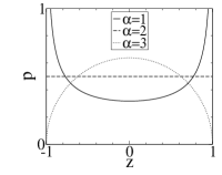
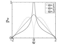
Figure 1: Stationary distributions in $z$- and $w$-space for different values of $\alpha$. Divergence emerges at the crossover $\alpha=2$ and is linked to the presence of immobile particles at trap borders.

At the crossover, $\alpha=2$, both distributions reduce to simple shapes: $p$ is flat and $p_{w}$ is triangular. Then for $\alpha<2$, both distributions develop divergences.

II.2 moment analysis

In this section, we briefly analyze even moments $\langle z^{2n}\rangle$ of a distribution $p(z)$ in Eq. (5). (Odd moments are zero due to even symmetry of $p$). The moments can be calculated directly from $p$ using $\langle z^{2n}\rangle=\int_{-1}^{1}dz\,p(z)z^{2n}$:

$$\langle z^{2n}\rangle=\frac{\Gamma\left(n+\frac{1}{2}\right)\Gamma\left(\frac{1}{2}+\frac{\alpha}{2}\right)}{\sqrt{\pi}\,\Gamma\left(\frac{1}{2}+\frac{\alpha}{2}+n\right)},~{}~{}~{}~{}\text{for }n=1,2,\dots$$ (10)

The moments are monotonically decreasing with increasing $n$. The infinite sum $\sum_{n=0}^{\infty}\langle z^{2n}\rangle$ can be evaluated exactly and is given by

$$\sum_{n=0}^{\infty}\langle z^{2n}\rangle=\begin{cases}\frac{\alpha-1}{\alpha-2}&\text{if $\alpha>2$}\\ \infty&\text{if $\alpha\leq 2$},\end{cases}$$ (11)

where at the crossover the sum is seen to diverge. By representing the infinite sum by its generating function, we can connect this behavior to the divergence in $p$:

$$\sum_{n=0}^{\infty}\langle z^{2n}\rangle=\left\langle\frac{1}{1-z^{2}}\right\rangle.$$

As particles accumulate at the borders, $z\to\pm 1$ and the above expression diverges. This explains the divergence of the sum in Eq. (11).

III RTP oscillator in 2D

We next consider an RTP oscillator with 1D geometry, $u=\frac{1}{2}Kx^{2}$, but embedded in 2D space. To set up the problem, we start with a Fokker-Planck equation for RTP particles in an arbitrary confinement:

$$\dot{\rho}=-\mbox{\boldmath$\nabla$}\cdot\left[\left(\mu{\bf F}+v_{0}{\bf n}\right)\rho\right]+\hat{L}\,\rho,$$ (12)

where ${\bf n}$ is the unit vector designating an orientation of the swimming velocity $v_{swim}=v_{0}{\bf n}$, in 2D defined as ${\bf n}=(\cos\theta,\sin\theta)$, where $\theta$ is the angle of the orientation. The evolution of ${\bf n}$ is governed by the operator $\hat{L}$ given by

$$\hat{L}\,\rho=\frac{1}{\tau}\left[-\rho+\frac{1}{2\pi}\int_{0}^{2\pi}d\theta\,\rho(x,\theta)\right].$$

The two terms imply that particles with a given orientation $\theta$ vanish with the rate $\tau^{-1}$ and reappear with the same rate at another location that depends on the marginal distribution

$$p=\int_{0}^{2\pi}d\theta\,\rho(x,\theta).$$

Note that $\int_{0}^{2\pi}d\theta\,\hat{L}\,\rho=0$. This condition is necessary if the total number of particles is to be conserved.

For $u=\frac{1}{2}Kx^{2}$, the external force is ${\bf F}=-Kx\,{\bf e}_{x}$. In a steady-state, only the component of ${\bf v}_{swim}$ in the $x$ direction is relevant, ${\bf v}_{swim}\cdot{\bf e}_{x}=v_{0}\cos\theta$. This results in an effectively one-dimensional system governed by the following stationary Fokker-Planck equation:

$$0=\frac{\partial}{\partial z}\left[\left(z-\cos\theta\right)\rho\right]-\alpha\rho+\frac{\alpha}{2\pi}p,$$ (13)

given in dimensionless units.

The above Fokker-Planck equation can be interpreted as representing RTP model in 1D with continuous distribution of velocities, and what constitutes a generalized RTP model Frydel21b . For a truly 1D RTP model, the distribution of swimming velocities is $P\propto\delta(v_{swim}+v_{0})+\delta(v_{swim}-v_{0})$. The Fokker-Planck equation in Eq. (13) represents a system for the following distribution of swimming velocoties: $P\propto 1/\sqrt{v_{0}^{2}-v_{swim}^{2}}$. See Appendix A in Frydel21a .

There is no straightforward procedure to reduce Eq. (14) to a differential equation for $p$ but it is possible to infer it from the moments of $p$. (How to calculate such moments will be demonstrated when we analyze a system in 3D). Because a moment formula in 2D was determined to have a similar structure to that in 1D, it was, in turn, possible to infer that a differential equation for $p$ should have the same structure as that for a system in 1D. See Eq. (4). For 2D, the differential equation for $p$ was determined to be Frydel22c

$$0=(1-2\alpha)zp-(1-z^{2})p^{\prime},$$ (14)

where the solution is a beta distribution

$$p(z)=A(1-z^{2})^{\alpha-\frac{1}{2}},$$ (15)

and where the normalization constant is given by

$$A=\frac{\Gamma\left(\alpha+1\right)}{\sqrt{\pi}\Gamma\left(\alpha+\frac{1}{2}\right)}.$$ (16)

III.1 distribution in $w$-space

For a system embedded in 2D, the velocity component in the $x$-direction is $v=-\mu Kx+v_{0}\cos\theta,$ in reduced units given by

$$w=-z+\cos\theta.$$ (17)

Compare this with Eq. (8).

The distribution $p_{w}$ can be obtained from Eq. (13) by substituting for $p$ with expression given in Eq. (15), followed by the change of variables $z=-w+\cos\theta$, followed by the integration over all orientations. This yields an inhomogeneous first order differential equation

$$(1-\alpha)p_{w}+wp_{w}^{\prime}=-\frac{\alpha}{2\pi}I,$$ (18)

where

$$I(w)=2A\int_{-1}^{1-w}ds\,\left[1-s^{2}\right]^{\alpha-\frac{1}{2}}\left[1-(s+w)^{2}\right]^{-\frac{1}{2}}.$$ (19)

The solution is a distribution defined on $[-2,2]$

$$p_{w}=\frac{\alpha}{2\pi}|w|^{\alpha-1}\left[\int_{|w|}^{2}dw^{\prime}\,w^{\prime-\alpha}I(w^{\prime})\right].$$ (20)

Although $p_{w}$ has a more complicated form compared to that in Eq. (9) for a system in 1D, its general structure remains similar. Divergence at $w=0$ comes from the factor $|w|^{\alpha-1}$, which signals the existence of nearly immobile particles for $\alpha>1$ and suggests the crossover at $\alpha=1$. This, however, is not corroborated by $p$ in Eq. (15), in which case divergences at the trap border emerge for $\alpha>1/2$.

The reason why divergences in $p$ disappear at a lower value of $\alpha$ is a result of averaging procedure used to obtain $p$ from $\rho$. Even if a distribution $\rho$ exhibits divergences up to $\alpha=1$, the averaging procedure $p=\int_{0}^{\pi}d\theta\,\rho$ smooths those divergences and effectively makes them disappear for $\alpha<1/2$. In Appendix (A) we analyze distributions $\rho$ in more detail to back up these claims.

In Fig. (2) we plot a number of different distributions $p_{w}$ for different values of $\alpha$ calculated using Eq. (20), where the integral is evaluated numerically. Those distributions are compared with those obtained from simulations. Simulations were carried out using the Euler method for updating particle positions:

$$x(t+\Delta t)=\left[v_{0}\cos\theta(t)-\mu Kx(t)\right]\Delta t,$$

with new orientation $\theta(t)$ selected after a time period selected randomly from the Poisson distribution $P\propto e^{-t/\tau}$. For comparison, in Fig. (2) we also plot the corresponding distributions $p$ below each $p_{w}$.

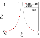
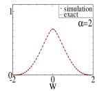
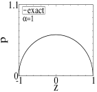
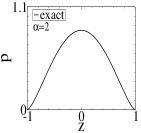
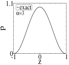
Figure 2: Distributions $p_{w}$ for different values of $\alpha$. Exact distributions (represented by lines) are obtained from Eq. (20). The circular symbols represent simulation data points. In addition, below each plot for $p_{w}$ we plot a corresponding distribution $p$ to emphasize qualitatively different behavior.

Unlike the distributions in Fig. (1) for the system in 1D, a peak at $w=0$ does not fall to zero for $\alpha$ above the crossover. We can calculate the height of $p_{w}$ at $w=0$ from Eq. (18) by setting $w$ to zero. This yields $p_{w}(0)=\frac{A}{2\pi}\frac{\alpha}{\alpha-1}I(0)$ which simplifies to

$$p_{w}(0)=\frac{1}{\alpha-1}\left[\frac{4^{\alpha}}{\pi}\frac{\alpha!\alpha!}{(2\alpha)!}\right]^{2}.$$ (21)

Rather than suddenly falling to zero for $\alpha>1$, the peak height at $w=0$ approaches zero algebraically as a function of $\alpha$.

For half integer values of $\alpha$, it is possible to obtain exact expression for $p_{w}$. Those expressions are derived in Appendix (B).

Note that the crossover in 2D occurs at $\alpha=1$ while that in 1D at $\alpha=2$. Yet if we recall the discussion below Eq. (3), the actual rate for a system in 1D is not $\alpha$ but $\alpha/2$. Therefore, considering the actual rates, the crossover in both dimensions occurs for the same rates.

III.2 moment analysis

The moments of the distribution $p(z)$ in Eq. (15) are obtained directly from the formula $\langle z^{2n}\rangle=\int_{-1}^{1}dz\,p(z)z^{2n}$:

$$\langle z^{2n}\rangle=\frac{\Gamma\left(n+\frac{1}{2}\right)\Gamma(\alpha+1)}{\sqrt{\pi}\Gamma(\alpha+n+1)}.$$ (22)

The moments generate a monotonically decreasing sequence whose infinite sum is

$$\sum_{n=0}^{\infty}\langle z^{2n}\rangle=\left\langle\frac{1}{1-z^{2}}\right\rangle=\begin{cases}\frac{2\alpha}{2\alpha-1}&\text{if $\alpha>\frac{1}{2}$}\\ \infty&\text{if $\alpha\leq\frac{1}{2}$}.\end{cases}$$ (23)

The sum diverges at $\alpha=\frac{1}{2}$. This is linked to divergences in $p$ and does not represent a crossover. An actual crossover is determined from the behavior of $p_{w}$.

IV RTP particles in 3D: linear harmonic trap

For RTP particles in a harmonic trap in 3D, theres is no available solution for a stationary distribution $p$. Instead of trying to obtain such a distribution directly, in this section we focus on how to obtain exact expressions fo the moments of $p$. The results of this section are the most important results of this work.

IV.1 moment analysis

The stationary Fokker-Planck equation for RTP particles in a harmonic potential $u=\frac{K}{2}x^{2}$ embedded in 3D is obtained from Eq. (12) for the force ${\bf F}=-Kx{\bf e}_{x}$ and

$$\hat{L}\,\rho=\frac{1}{\tau}\left[-\rho+\frac{1}{2}\int_{0}^{\pi}d\theta\,\sin\theta\,\rho(x,\theta)\right].$$

The resulting equation in reduced units is

$$0=\frac{\partial}{\partial z}\left[\left(z-\cos\theta\right)\rho\right]-\alpha\rho+\frac{\alpha}{2}p,$$ (24)

with the marginal distribution defined as

$$p(z)=\int_{0}^{\pi}d\theta\,\sin\theta\,\rho(z,\theta).$$ (25)

The Fokker-Planck equation in Eq. (24) can be transformed into the following recurrence relation:

$$A_{l,m}=\frac{\alpha}{l+\alpha}A_{l,0}A_{0,m}+\frac{l}{l+\alpha}A_{l-1,m+1}$$ (26)

where

$$A_{l,m}=\langle z^{l}\cos^{m}\theta\rangle,$$

and the angular brackets indicate averaging procedure defined as $\langle\dots\rangle=\int_{-1}^{1}dz\int_{0}^{\pi}d\theta\,\rho\sin\theta(\dots)$.

The recurrence relation reflects the structure of the differential equation from which it was obtained: it is first order, linear, with variable coefficients. The relation was obtained by multiplying the Fokker-Planck equation by $z^{l}\cos^{m}\theta$ followed by integration $\int_{-1}^{1}dz\int_{0}^{\pi}d\theta\,\sin\theta$ and written in its final form using integration by parts.

Since $A_{l,0}=\langle z^{l}\rangle$, solving the recurrence relation would permit us to obtain moments. The initial condition of the recurrence relation is provided by the terms $A_{0,m}$ which are easily evaluated

$$A_{0.m}=\frac{1}{2}\int_{0}^{\pi}d\theta\,\sin\theta\cos^{m}\theta=\begin{cases}\frac{1}{m+1}&\text{if $m$ even}\\ 0&\text{if $m$ odd}.\end{cases}$$

The recurrence relation cannot be solved for an arbitrary $A_{l,m}$. Nonetheless, it is possible to reduce the relation to another recurrence relation in terms of $A_{2n,0}=\langle z^{2n}\rangle$ only:

$$\langle z^{2n}\rangle=\frac{\alpha}{2n}\sum_{k=0}^{n-1}\frac{\langle z^{2k}\rangle}{2n-2k+1}\frac{(2k+1)_{\alpha-1}}{(2n+1)_{\alpha-1}}.$$ (27)

where $(x)_{n}=\frac{\Gamma(x+n)}{\Gamma(x)}$ is the falling factorial.

The recurrence relation in Eq. (27) is the central result of this section. Although it does not provide an exact expression for an arbitrary moment, it provides an analytically tractable procedure for obtaining such an expression recursively. A number of initial even moments generated from the recurrence relation in Eq. (27) are given in Table (1).

$\langle z^{2}\rangle=\frac{1}{3}\frac{1}{1+\alpha}$

$\langle z^{4}\rangle=\frac{1}{15}\frac{18+5\alpha}{(1+\alpha)(2+\alpha)(3+\alpha)}$

$\langle z^{6}\rangle=\frac{1}{63}\frac{1080+378\alpha+35\alpha^{2}}{(\alpha+1)(\alpha+2)(\alpha+3)(\alpha+4)(\alpha+5)}$

$\langle z^{8}\rangle=\frac{1}{135}\frac{75600+28404\alpha+3780\alpha^{2}+175\alpha^{3}}{(\alpha+1)(\alpha+2)(\alpha+3)(\alpha+4)(\alpha+5)(\alpha+6)(\alpha+7)}$

$\langle z^{10}\rangle=\frac{1}{99}\frac{3265920+1259280\alpha+193644\alpha^{2}+13860\alpha^{3}+385\alpha^{4}}{(\alpha+1)(\alpha+2)(\alpha+3)(\alpha+4)(\alpha+5)(\alpha+6)(\alpha+7)(\alpha+8)(\alpha+9)}$

Table 1: Moments of a stationary distribution $p$ obtained from a recurrence relation in Eq. (27).

By examining Table (1), we can verify that for $\alpha=0$ the moments reduce to a simple general formula $\langle z^{2n}\rangle=\frac{1}{2n+1}$ that can be linked to a uniform distribution where $\langle z^{2n}\rangle=\frac{1}{2}\int_{-1}^{1}dz\,z^{2n}$. This means that for finite $\alpha$, $p$ can only be convex which, in turn, implies the absence of divergences at the trap borders.

To understand how a flat distribution arises for $\alpha=0$ we should understand that for $\alpha=0$ all particles are immobile and trapped at $z=\cos\theta$, where the swimming velocity and the velocity due to harmonic potential cancel one another. As a result $\rho=\frac{1}{2}\delta(z-\cos\theta)$. Averaged over all orientations, this yields:

$$\lim_{\alpha\to 0}p(z)=\frac{1}{2}\int_{0}^{\pi}d\theta\,\sin\theta\,\delta(z-\cos\theta)=\frac{1}{2}.$$ (28)

The averaging procedure completely smooths out the delta distribution.

In the Table (2), we compare the second and fourth moments calculated for different dimension. For 1D and 2D, these moments are obtained from the formulas in Eq. (10) and Eq. (22). The tendency is that an increased dimensionality reduces the value of a given moment. The best way to understand this reduction is to think of each system as one-dimensional with different distributions of swimming velocities (for a potential $u=\frac{K}{2}x^{2}$ we actually consider the projection of a swimming velocity along the $x$-axis and not the true swimming velocity).

	$\langle z^{2}\rangle$	$~{}~{}~{}~{}~{}~{}~{}~{}~{}\langle z^{4}\rangle$
1D	$\frac{1}{1+\alpha}$	$\frac{3}{(1+\alpha)(3+\alpha)}$
2D	$\frac{1}{2}\frac{1}{1+\alpha}$	$\frac{1}{4}\frac{3}{(1+\alpha)(2+\alpha)}$
3D	$\frac{1}{3}\frac{1}{1+\alpha}$	$\frac{1}{15}\frac{18+5\alpha}{(1+\alpha)(2+\alpha)(3+\alpha)}$

Table 2: Second and fourth moments of the distribution $p$ in different dimensions.

IV.2 distribution in $w$-space

To obtain a distribution in $w$-space we follow a similar procedure to that used in Sec. (III.1). We transform Eq. (24) using the change of variables $z=-w+\cos\theta$. The resulting equation is then integrated over all orientations. The procedure yields the first order inhomogeneous differential equation:

$$0=(1-\alpha)p_{w}+wp_{w}^{\prime}+\frac{\alpha}{2}\int_{-1}^{1-w}ds\,p(s),$$ (29)

for which the solution is

$$p_{w}=\frac{\alpha}{2}|w|^{\alpha-1}\left[\int_{|w|}^{2}dw^{\prime}\,w^{\prime-\alpha}\int_{-1}^{1-w^{\prime}}ds\,p(s)\right].$$ (30)

The solution permits us to obtain $p_{w}$ from $p$. The difference between this result and that in Eq. (20) is that here we do not have the exact expression for $p$.

Even without knowing $p$, Eq. (29) can be used to calculate $p_{w}(0)$ by setting $w=0$. This yields

$$p_{w}(0)=\frac{1}{2}\frac{\alpha}{\alpha-1}.$$ (31)

The expression diverges at $\alpha=1$, indicating a divergence in $p_{w}$ and the presence of nearly immobile particles. Compared with a similar result in Eq. (21) for a system in 2D, we see that the divergence occurs at the same value of $\alpha$. This means that the location of the crossover is independent of the system dimension.

In Fig. (3) we plot $p_{w}$ for different values of $\alpha$ obtained using Eq. (30). The integrals are calculated numerically and $p$ is calculated from the moments as explained in the next section.

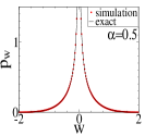
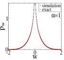
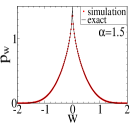
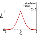
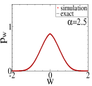
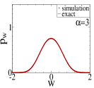
Figure 3: Distributions $p_{w}$ calculated from $p$ using numerically evaluated Eq. (30). The height of the peak at $w=0$ for $\alpha>1$ is given by Eq. (21).

IV.3 recovering $p$ from moments

The recurrence relation in Eq. (27) permits fast computation of an arbitrary number of even moments of $p$. In this section we present a procedure for recovering a distribution $p$ from the moments based on the Fourier-Legendre expansion,

$$p(z)=\sum_{n=0}^{\infty}a_{n}P_{2n}(z),$$ (32)

where $P_{m}$ are Legendre (orthogonal) polynomials. Like $p$, Legendre polynomials are defined on $[-1,1]$. Due to even symmetry of $p$, only even Legendre polynomials $P_{2n}$ are required:

$$P_{2n}=2^{2n}\sum_{k=0}^{n}\frac{z^{2k}\,\Gamma\left(k+n+\frac{1}{2}\right)}{(2k)!(2n-2k)!\,\Gamma\left(k-n+\frac{1}{2}\right)}.$$ (33)

The coefficients $a_{n}$ in Eq. (32) can be determined from the orthogonality relation $\int_{-1}^{1}dz\,P_{n}P_{m}=\frac{2}{2n+1}\delta_{mn}$ which leads to

$$a_{n}=\frac{4n+1}{2}\int_{-1}^{1}dz\,P_{2n}(z)p(z),$$ (34)

and in combination with Eq. (33) yields

$$a_{n}=\frac{4n+1}{2}\left[2^{2n}\sum_{k=0}^{n}\frac{\langle z^{2k}\rangle\,\Gamma\left(k+n+\frac{1}{2}\right)}{(2k)!(2n-2k)!\,\Gamma\left(k-n+\frac{1}{2}\right)}\right].$$ (35)

The expansion in Eq. (32) together with the coefficients in Eq. (35) provides an exact formula for recovering $p$ in terms of moments obtained from Eq. (27). Initial coefficients $a_{n}$ are listed in Table (3).

$a_{0}=\frac{1}{2}$

$a_{1}=-\frac{5}{4}\frac{\alpha}{\alpha+1}$

$a_{2}=-\frac{3}{16}\frac{16\alpha-24\alpha^{2}-9\alpha^{3}}{(\alpha+1)(\alpha+2)(\alpha+3)}$

$a_{3}=-\frac{13}{96}\frac{288-496\alpha+120\alpha^{2}+120\alpha^{3}+15\alpha^{4}}{(\alpha+1)(\alpha+2)(\alpha+3)(\alpha+4)(\alpha+5)}$

$a_{4}=-\frac{17}{768}\frac{55296-105984\alpha+49280\alpha^{2}+8512\alpha^{3}-6720\alpha^{4}-1680\alpha^{5}-105\alpha^{6}}{(\alpha+1)(\alpha+2)(\alpha+3)(\alpha+4)(\alpha+5)(\alpha+6)(\alpha+7)}$

Table 3: Coefficients for the Fourier-Legendre series in in Eq. (32).

Note that by setting $\alpha=0$, $a_{0}=1/2$ and all the remaining coefficients $a_{n}$ are zero. This implies a uniform distribution in agreement with the results in Eq. (28) for the same limit.

Recovered distributions obtained from a truncated Fourier-Legendre series $p=\sum_{n=0}^{N_{c}}a_{n}P_{2n}(z)$ for $N_{c}=10$ are shown in Fig. (4).

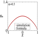
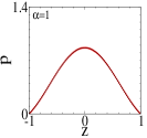
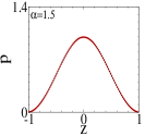
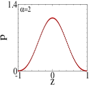
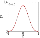
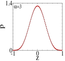
Figure 4: Distributions $p$ calculated using the truncated Fourier-Legendre series $p=\sum_{n=0}^{N_{c}}a_{n}P_{2n}(z)$, for $N_{c}=10$ and $a_{n}$ defined in Eq. (35).

The truncated series shows a very good agreement with $p$ obtained from simulations. The larger the $\alpha$, the less terms of expansion are needed. It is generally recognized that the delta and square distributions are not well approximated by the series. But since only the distribution at $\alpha=0$ is flat (and does not need to be approximated), this limitation does not apply to our situation.

V Thermal fluctuations

Up to this point, all the analysis and results were done at zero temperature. To incorporate thermal fluctuations, we use a known result that for particles in a harmonic trap a stationary distribution of active particles in a thermal bath can be represented as convolution Frydel22c , for a system with 1D geometry given by

$$p_{T}(x)=\int d{x}^{\prime}\,p(x^{\prime})p_{eq}({x}-{x}^{\prime}),$$ (36)

where $p_{eq}({x})=\sqrt{\frac{\mu K}{2\pi D}}e^{-\mu Kx^{2}/2D}$ is the Boltzmann distribution of passive particles in a harmonic trap, and $p$ is the stationary distribution at zero temperature.

A convolution construction applies to any combination of independent random processes book08 ; book19 . Generally, however, confinement leads to correlations between random processes as it gives rise to nonlinear terms in the Langevin equation, even if these processes are originally independent. The exception is a harmonic potential whose force is linear and it does not introduce nonlinear terms. See Appendix (C) for further discussion regarding this point.

Using Eq. (36), the moments of the distribution $p_{T}$ are defined as

$$\langle z^{2n}\rangle_{T}=\int_{-\infty}^{\infty}dz\,z^{2n}\int_{-1}^{1}dz^{\prime}\,p(z^{\prime})p_{eq}(z-z^{\prime}),$$ (37)

assuming dimensionless units. Then using the identity $z^{2n}=\left[(z-z^{\prime})+z^{\prime}\right]^{2n}$ together with binomial expansion, Eq. (37) yields

$$\langle z^{2n}\rangle_{T}=\sum_{k=0}^{n}\frac{(2n)!}{(2k)!(2n-2k)!}\langle z^{2n-2k}\rangle\langle z^{2k}\rangle_{eq}.$$ (38)

And since moments $\langle z^{2k}\rangle_{eq}$ can be calculated using the Boltzmann distribution, we finally get

$$\langle z^{2n}\rangle_{T}=\sum_{k=0}^{n}\frac{(2n)!B^{k}}{2^{k}k!(2n-2k)!}\langle z^{2n-2k}\rangle,$$ (39)

where $B=\frac{\mu K}{v_{0}^{2}}D$ is the dimensionless diffusion constant.

Note that the moments for a finite temperature are given as an expansion in terms of moments at zero temperature. Since all terms in the expansion are positive, the effect of temperature is to increase the value of all the moments.

Using Eq. (38), the initial moments are given by

$$\langle z^{2}\rangle_{T}=\langle z^{2}\rangle+\langle z^{2}\rangle_{eq}$$

$$\langle z^{4}\rangle_{T}=\langle z^{4}\rangle+6\langle z^{2}\rangle\langle z^{2}\rangle_{eq}+\langle z^{4}\rangle_{eq}$$

$$\langle z^{6}\rangle_{T}=\langle z^{6}\rangle+15\langle z^{4}\rangle\langle z^{2}\rangle_{eq}+15\langle z^{2}\rangle\langle z^{4}\rangle_{eq}+\langle z^{6}\rangle_{eq}$$

Note that the two contributions of the second moment are completely additive. Using Eq. (39), the initial moments in the actual units are given by

$$\langle x^{2}\rangle_{T}=\langle x^{2}\rangle+\frac{k_{B}T}{K}$$

$$\langle x^{4}\rangle_{T}=\langle x^{4}\rangle+6\langle x^{2}\rangle\frac{k_{B}T}{K}+3\left(\frac{k_{B}T}{K}\right)^{2}$$

$$\langle x^{6}\rangle_{T}=\langle x^{6}\rangle+15\langle x^{4}\rangle\frac{k_{B}T}{K}+45\langle z^{2}\rangle\left(\frac{k_{B}T}{K}\right)^{2}+15\left(\frac{k_{B}T}{K}\right)^{3}$$

where we used $D=\mu k_{B}T$. This result shows more clearly contribution of the temperature.

VI Isotropic harmonic trap

The previous analysis was done for a harmonic potential in a single direction, $u=\frac{1}{2}Kx^{2}$, and it is not clear how and if the obtained results apply to an isotropic potential $u=\frac{1}{2}Kr^{2}$. In this section we extend the previous results to such an isotropic potential.

To establish a relation between moments for a linear potential, $\langle x^{2n}\rangle$, and the moments of an isotropic potential, $\langle r^{2n}\rangle$, we consider first the Boltzmann distribution, $p_{eq}(r)\propto e^{-\frac{\mu Kr^{2}}{2D}}$ to see how respective moments are related in this case. For an arbitrary dimension $d$, the moments are easily evaluated and are given by

$$\langle r^{2n}\rangle=\left(\frac{2D}{\mu K}\right)^{n}\frac{\Gamma\left(\frac{d}{2}+n\right)}{\Gamma\left(\frac{d}{2}\right)}.~{}~{}~{}~{}$$ (42)

Note that $\langle x^{2n}\rangle=\langle r^{2n}\rangle_{d=1}$ so that we can write

$$\langle x^{2n}\rangle=\left(\frac{2D}{\mu K}\right)^{n}\frac{\Gamma\left(\frac{1}{2}+n\right)}{\Gamma\left(\frac{1}{2}\right)}.$$

This permits us to represent Eq. (42) as

$$\langle r^{2n}\rangle=\frac{\Gamma\left(\frac{1}{2}\right)\Gamma\left(n+\frac{d}{2}\right)}{\Gamma\left(\frac{d}{2}\right)\Gamma\left(n+\frac{1}{2}\right)}\langle x^{2n}\rangle,$$ (43)

which establishes a relation between $\langle x^{2n}\rangle$ and $\langle r^{2n}\rangle$.

The relation in Eq. (43) was derived by considering the equilibrium distribution. We next verify that the same relation applies for RTP particles. Since we know that a stationary distribution of RTP particles in an isotropic harmonic potential in 2D is Frydel22c

$$p(s)=\frac{\alpha}{\pi}(1-s^{2})^{\alpha-1},$$ (44)

where we introduce a dimensionless variable $s=\mu Kr/v_{0}$, we can calculate the moments $\langle s^{2n}\rangle=\int_{0}^{1}ds\,2\pi sp(s)s^{2n}$ which can then compared with the moments in Eq. (22) for a linear harmonic potential. The comparison recovers the formula in Eq. (43) for $d=2$.

The verification of Eq. (43) for $d=3$ is more intricate and the details are relegated to Appendix. But it leads to the following relation

$$\langle r^{2n}\rangle=(2n+1)\langle x^{2n}\rangle$$ (45)

which also agrees with Eq. (43) for $d=3$. Consequently, the relation in Eq. (43) is general and applies to passive and RTP particles in a harmonic potential.

Combining the relation in Eq. (45) with the recurrence relation in Eq. (27), we next get the recurrence relation for the moments of a stationary distribution $p(s)$ in an isotropic harmonic potential in 3D

$$\langle s^{2n}\rangle=\frac{\alpha}{2n}\sum_{k=0}^{n-1}\frac{\langle s^{2k}\rangle}{2n-2k+1}\frac{(2k+2)_{\alpha-2}}{(2n+2)_{\alpha-2}}.$$ (46)

The central result of this section is Eq. (43), which establishes a relation between moments $\langle r^{2n}\rangle$ and $\langle x^{2n}\rangle$. This relation is then used to determine the recurrence relation in Eq. (46).

VI.1 recovering $p$ from moments

To recover a distribution $p(s)$ for an isotropic harmonic trap in 3D from the moments in Eq. (46), we are going to use the Fourier-Legendre expansion, as was done in Sec. (IV.3). However, since the normalized function is $4\pi s^{2}p(s)$, we expand this quantity rather than $p(s)$. The resulting expansion is

$$4\pi s^{2}p(s)=2\sum_{n=0}^{\infty}a_{n}P_{2n}(s).$$ (47)

The factor $2$ in front of the sum comes from the fact that $p(s)$ is defined on $[0,1]$ while the polynomials $P_{n}$ are defined on $[-1,1]$.

The coefficients $a_{n}$ in the expansion are the same as those in Eq. (35) but defined in terms of $\langle s^{2n}\rangle$:

$$a_{n}=\frac{4n+1}{2}\left[2^{2n}\sum_{k=0}^{n}\frac{\langle s^{2k}\rangle\,\Gamma\left(k+n+\frac{1}{2}\right)}{(2k)!(2n-2k)!\,\Gamma\left(k-n+\frac{1}{2}\right)}\right].$$ (48)

Fig. (5) compares distributions $p(s)$ obtained using the truncated Fourier-Legendre expansion with those obtained from a simulation.

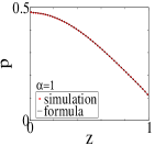
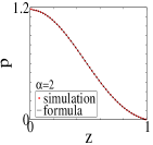
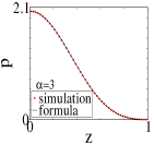
Figure 5: Distributions $p$ calculated using the truncated Fourier-Legendre series $p(s)=\frac{1}{2\pi s^{2}}\sum_{n=0}^{N_{c}}a_{n}P_{2n}(s)$, for $N_{c}=10$ and $a_{n}$ defined in Eq. (48).

The plots indicate that for $\alpha>1$ the distributions $p(s)$ vanish at $s=1$, confirming $\alpha=1$ to be a point of crossover.

VII Summary and conclusion

The central result of this work is the recurrence relation for generating moments of a stationary distribution $p$ for RTP particles in a harmonic trap in three-dimensions. As there is no available exact expression for $p$ in this dimension, this approach provides an alternative route with analytical tractability.

For the potential $u=\frac{1}{2}Kx^{2}$ the recurrence relation in dimensionless parameters is given in Eq. (27). This result is specific for a system embedded in 3D space but it can be generalized to any dimension. A generalized form, valid for any dimension $d$, is given by

$$\langle z^{2n}\rangle=\frac{\alpha}{2n}\sum_{k=0}^{n-1}\langle z^{2k}\rangle\frac{(2k+1)_{\alpha-1}}{(2n+1)_{\alpha-1}}c_{2n-2k},$$ (49)

where $c_{2n}=A_{0,2n}$ and is given by

$$c_{2n}=\frac{\Gamma\left(\frac{d}{2}\right)\Gamma\left(n+\frac{1}{2}\right)}{\Gamma\left(\frac{1}{2}\right)\Gamma\left(n+\frac{d}{2}\right)}.$$ (50)

Note that the parameter of dimensionality only enters via the coefficient $c_{2n}$.

The general formula in Eq. (49) can be verified. For $d=3$, it recovers the result in Eq. (27). For $d=1$ and $d=2$, Eq. (49) can be solved for $\langle z^{2n}\rangle$, with solutions found to agree with Eq. (10) and Eq. (22).

Using the relation in Eq. (43), we can obtain a similar general recurrence relation for the moments of a stationary distribution for an isotropic harmonic potential:

$$\langle s^{2n}\rangle=\frac{\alpha}{2n}\sum_{k=0}^{n-1}\langle s^{2k}\rangle\frac{(2k+2)_{\alpha-2}}{(2n+2)_{\alpha-2}}c_{2n-2k}.$$ (51)

The general recurrence formulas in Eq. (49) and in Eq. (51) permit us to better understand the role of system dimension. The fact that in $d=3$ the recurrence relation cannot be solved implies a more complex functional form of $p(z)$. This might help to explain why in this dimension there is no corresponding trivial differential equation for $p(z)$ Frydel22c . The idea of a function without a corresponding differential equation was first put forward in 1887 by Hölder Holder87 who considered an Euler gamma function. In 1900 Hilbert conjectured that the Riemann zeta function is another example Hilbert . In 1920’s this conjecture was proven to be correct Ostrowski , and in 2015, it was shown that the Riemann zeta function formally satisfies an infinite order linear differential equation Gorder .

Another important aspect of this work is the determination of a crossover at $\alpha=1$, regardless of a system dimension. The importance of a crossover is that it indicates when to expect the presence of "nearly immobile" particles accumulated near a trap border. Since $\alpha=\frac{1}{\tau\mu K}$ is the ratio of two time scales, the persistence time $\tau$ during which an active particle retains its orientation, and the time a particle needs to reach a trap border $1/\mu K$, the crossover value gives a way to predict the shape of a distribution once we know $\alpha$. If a typical persistence time for a E. Coli is $\tau\sim 1s$ and a typical velocity $v_{0}=40\mu s^{-1}$ book04 , then we should expect the trap size to be $v_{0}/\mu K\lesssim 40\mu$ in order to see accumulation of particles at a trap border.

The most obvious extension of the "recurrence" method is to apply it to other types of active particles, for example, the ABP model. Since the Fokker-Planck equation for the ABP system is different, one expects a different recurrence relation. It is not clear if the methodology is extendeable to other types of external potentials or simple interactive systems such as the Kuramoto model Frydel21 , known to undergoe a phase transition, or the one-dimensional asymmetric exclusion process mode PRL06 ; PRE21 .

VIII DATA AVAILABILITY

The data that support the findings of this study are available from the corresponding author upon reasonable request.

Appendix A exact distributions $\rho$ for RTP particles in a harmonic trap in 2D

In this section we solve the Fokker-Planck equation in Eq. (13) for $\rho$ by substituting for $p$ the expression in Eq. (15). This permits us to posit Eq. (13) as a first order inhomogeneous differential equation:

$$0=(z-\cos\theta)\rho^{\prime}+(1-\alpha)\rho+\frac{\alpha A}{2\pi}(1-z^{2})^{\alpha-\frac{1}{2}}.$$ (52)

By multiplying the above equation by the integrating factor

$$e^{\int_{-1}^{z}dy\,\frac{1-\alpha}{y-\cos\theta}}=\left(\frac{\cos\theta+1}{\cos\theta-z}\right)^{\alpha-1},$$

the solution can be represented as

$$\rho_{L}=A\frac{\alpha}{2\pi}\left|\cos\theta-z\right|^{\alpha-1}\int_{-1}^{z}dz^{\prime}\,(1-z^{\prime 2})^{\alpha-\frac{1}{2}}\left|\cos\theta-z^{\prime}\right|^{-\alpha},$$ (53)

for the domain $-1<z<\cos\theta$, and

$$\rho_{R}=A\frac{\alpha}{2\pi}\left|\cos\theta-z\right|^{\alpha-1}\int_{z}^{1}dz^{\prime}\,(1-z^{\prime 2})^{\alpha-\frac{1}{2}}\left|\cos\theta-z^{\prime}\right|^{-\alpha},$$ (54)

for the domain $\cos\theta<z<1$.

The difference between the solutions in each domain lies in the limits of an integral. The limits ensure that the distribution in Eq. (53) vanishes at $z=-1$ and the distribution in Eq. (54) vanishes at $z=1$. Except for $\rho(z,0)$ and $\rho(z,\pi)$, for any other orientation $\theta$, $\rho$ vanishes at both $z=\pm 1$. Divergence in $\rho$ comes from the pre-factor $\left|\cos\theta-z\right|^{\alpha-1}$. This implies that the divergence for each $\rho$ is localized at $z=\cos\theta$ and the crossover corresponds to $\alpha=1$ — as verified by the behavior of $p_{w}$.

The height of the distribution at $z=\cos\theta$ for $\alpha>1$, when a divergence disappears, can easily be evaluated from Eq. (52):

$$\rho(z=\cos\theta,\theta)=\frac{A}{2\pi}\frac{\alpha}{\alpha-1}(1-\cos^{2}\theta)^{\alpha-\frac{1}{2}}.$$ (55)

Note that the point $z=\cos\theta$ does not represent a maximal value of $\rho$ for $\alpha>1$. The actual peak is shifted toward $z=0$ as shown in Fig. (6).

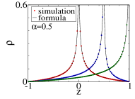
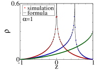
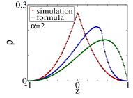
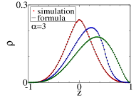
Figure 6: Distributions $\rho(z,\theta)$ for three swimming orientations: $\cos\theta=0,\frac{1}{2},1$ — red, blue , green points, respectively. Each distribution integrates to $\int_{-1}^{1}dz\,\rho(z,\theta)=\frac{1}{2\pi}$. All circular symbols represent simulation data points, and the lines represent exact results obtained using Eq. (53) and Eq. (54).

The solutions in Eq. (53) and Eq. (54) for $\cos\theta=0$ become

$$\rho\propto|z|^{\alpha-1}\left(1-z^{2}\right)^{\alpha+\frac{1}{2}}\,_{2}F_{1}\left(\frac{\alpha+1}{2},\frac{2\alpha+1}{2},\frac{2\alpha+3}{2},1-z^{2}\right),$$ (56)

and for $\cos\theta=\pm 1$

$$\rho\propto\left(1-z^{2}\right)^{\alpha-1}(1\pm z)^{\frac{3}{2}}\,_{2}F_{1}\left(\frac{1}{2},\frac{2\alpha+1}{2},\frac{2\alpha+3}{2},\frac{1\pm z}{2}\right).$$ (57)

Both solutions are for the full domain $[-1,1]$.

It is interesting to compare the distributions given above with the distributions for the three-state RTP model in Basu20 . The three-state RTP model is an extension of the RTP model in 1D considered in Sec. (II) that includes the zero swimming velocity, $v_{swim}=-v_{0},0,v_{0}$. The resulting stationary distribution $p$ has three divergences at $z=-1,0,1$. The divergences at different position correspond to different swimming velocities, for example, the divergence at $z=0$ is linked to particles with zero velocity. The exact solutions for $p_{\pm}$ and $p_{0}$ are expressed in terms of the hypergeometric functions, similar to the solutions in Eq. (56) and Eq. (57). This suggests that the analytical complexity quickly rises if we move away from the two-state model.

In Sec. (III.1) we calculated distributions in $w$-space for all particles, that is, averaged over all orientations. But knowing $\rho$, it is now possible to calculate distributions in $w$-space corresponding to a given orientation. To obtain such distributions, we transform $\rho$ using the change of variables $z=-w+\cos\theta$.

The distributions $\rho(w,\theta)$ are plotted in Fig. (7).

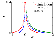
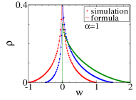
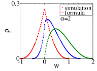
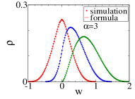
Figure 7: Distributions $\rho(w,\theta)$ for three swimming orientations: $\cos\theta=0,\frac{1}{2},1$ — red, blue , green points, respectively. All circular symbols represent simulation data points, and the lines represent exact results obtained using Eq. (53) and Eq. (54).

Note that all divergences, regardless of the orientation of a motion, are at $w=0$ which signals the presence of nearly immobile particles. For $\alpha>1$, nearly immobile particles disappear, manifested by the disappearance of divergences. Another observation is that for $\alpha>1$, all the peaks, originally at $w=0$, start to shift away from $w=0$ toward $w\to\cos\theta$, that is, the value of a swimming velocity of particles with orientation $\theta$. Only distribution with orientation $\theta=\pm\pi/2$ are centered around $w=0$.

Note that the domain of a distribution $\rho(w,\theta)$ depends on $\cos\theta$ and is given by $w\in(-1+\cos\theta,1+\cos\theta)$.

Appendix B exact results for $p_{w}$

For half integer values of $\alpha$, the integral in Eq. (20) can be evaluated exactly. For the first three values, $\alpha=\frac{1}{2},\frac{3}{2},\frac{5}{2}$, the distribution can be represented as

$$p_{w}=\frac{a_{\alpha}}{\pi}\sqrt{\frac{2-w}{w}}+b_{\alpha}\left[\frac{\sin^{-1}(1-w)}{2\pi}+\frac{1}{4}\right],$$ (58)

where $a_{\alpha}$ and $b_{\alpha}$ are polynomials given in Table (4).

$\alpha$	$a_{\alpha}$	$b_{\alpha}$
${1}/{2}$	$1$	$-1$
${3}/{2}$	$-\left(7w+13w^{2}\right)/8$	$\left(9+6w^{2}\right)/4$
${5}/{2}$	$\left(75w+537w^{2}+178w^{3}+298w^{4}\right)/128$	$\left(75-600w^{2}-120w^{4}\right)/64$

Table 4: Polynomials $a_{\alpha}$ and $b_{\alpha}$ for the formula in Eq. (58).

Fig. (8) compares these analytical results with simulation data points.

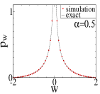
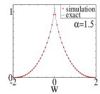
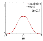
Figure 8: Distributions $p_{w}$ for different values of $\alpha$. Exact distributions (represented by lines) are obtained from Eq. (58). The circular symbols represent simulation data points.

Appendix C Convolution of probability distributions

To show explicitly that the convolution of probability distributions works for particles in a harmonic potential $u=Kr^{2}/2$ whose dynamics is governed by $N$ independent forces ${\bf f}_{i}$, we consider the Langevin equation. For an unconfined system the Langevin equation is

$$\dot{\bf r}=\mu\sum_{i=1}^{N}{\bf f}_{i},$$ (59)

where $\langle{\bf f}_{i}(t)\cdot{\bf f}_{j}(t^{\prime})\rangle=f_{i}^{2}\delta_{ij}\,\tau_{i}^{-1}e^{-|t-t^{\prime}|/\tau_{i}},$ where we assumed exponential memory such that in the limit $\tau_{i}\to 0$, $\tau_{i}^{-1}e^{-|t-t^{\prime}|/\tau_{i}}\to\delta(t-t^{\prime}).$ For particles in a harmonic trap the Langevin equation is

$$\dot{\bf r}=\mu\sum_{i=1}^{N}{\bf f}_{i}-\mu K{\bf r},$$ (60)

and can be solved to yield

$${\bf r}=\mu\sum_{i=1}^{N}\int_{-\infty}^{t}ds\,e^{-\mu K(t-s)}{\bf f}_{i}(s).$$ (61)

Using the above solution, the Langevin equation in Eq. (60) can be represented as

$$\dot{\bf r}=\mu\sum_{i=1}^{N}\bar{\bf f}_{i}$$ (62)

where the new forces are defined as

$$\bar{\bf f}_{i}={\bf f}_{i}-\mu K\int_{-\infty}^{t}ds\,e^{-\mu K(t-s)}{\bf f}_{i}(s).$$ (63)

The new forces can be shows to be independent:

$$\langle\bar{\bf f}_{i}(t)\cdot\bar{\bf f}_{j}(t^{\prime})\rangle=f_{i}^{2}\delta_{ij}M(t-t^{\prime}),$$ (64)

where $M$ is a resulting new memory function.

Appendix D computation of moments for an isotropic harmonic potential in 3D

In this section we provide an explicit verification of the relation in Eq. (43) for the RTP particles in a harmonic trap in 3D. We start with the stationary FP equation

$$0=\mbox{\boldmath$\nabla$}\cdot\left[\left(\mu K{\bf r}-v_{0}{\bf n}\right)\rho\right]+\hat{L}\,\rho,$$

where the operator $\hat{L}$ for the RTP model in 3D is given by

$$\hat{L}\,\rho=\frac{1}{\tau}\left[-\rho+\frac{1}{2}\int_{0}^{\pi}d\theta\,\sin\theta\rho(x,\theta)\right].$$

Since $\rho$ depends on the relative orientation of the vectors ${\bf r}$ and ${\bf n}$, we fix ${\bf n}$ along the $x$-axis, ${\bf n}={\bf e}_{x}$, and the FP equation becomes

$$0=\mu K{\bf r}\cdot\mbox{\boldmath$\nabla$}\rho+\mu K\rho(\mbox{\boldmath$\nabla$}\cdot{\bf r})-v_{0}\frac{\partial\rho}{\partial x}+\hat{L}\,\rho.$$ (65)

In spherical coordinates: $\frac{\partial\rho}{\partial x}=\cos\theta\frac{\partial\rho}{\partial r}-\frac{\sin\theta}{r}\frac{\partial\rho}{\partial\theta}$, ${\bf r}\cdot\mbox{\boldmath$\nabla$}\rho=r\frac{\partial\rho}{\partial r}$, and $\mbox{\boldmath$\nabla$}\cdot{\bf r}=d$. The FP equation in reduced units $s=\mu Kr/v_{0}$ can now be expressed

$$0=s\rho^{\prime}+3\rho-\cos\theta\rho^{\prime}+\frac{\sin\theta}{s}\frac{\partial\rho}{\partial\theta}-\alpha\rho+\frac{\alpha}{2}p,$$ (66)

where

$$p=\int_{0}^{\pi}d\theta\,\sin\theta\rho(z,\theta).$$

By multiplying the above equation by $s^{l}\cos^{m}\theta$ and then integrating it as $4\pi\int_{0}^{\infty}ds\,s^{2}\int_{0}^{\pi}d\theta\,\sin\theta$, we get the following recurrence relation:

$$B_{l,m}=\frac{\alpha}{l+\alpha}B_{l,0}B_{0,m}+\frac{l-m}{l+\alpha}B_{l-1,m+1}+\frac{m}{l+\alpha}B_{l-1,m-1}.$$ (67)

where $B_{l,m}=\langle s^{l}\cos^{m}\theta\rangle,$ and the initial condition is $B_{0,0}=1.$ The recurrence relation in Eq. (67) is used to solve for $B_{2n,0}=\langle s^{2n}\rangle$ that satisfies the relation

$$\langle s^{2n}\rangle=(2n+1)\langle z^{2n}\rangle,$$ (68)

where $\langle z^{2n}\rangle$ is defined in Eq. (27). Consequently, the relation in Eq. (43) is verified for the RTP model.

References

- (1) J. Tailleur and M. E. Cates, Statistical Mechanics of Interacting Run-and-Tumble Bacteria, Phys. Rev. Lett. 100, 218103 (2008).
- (2) J. Tailleur and M. E. Cates, Sedimentation, trapping, and rectification of dilute bacteria, Europhys. Lett. 86, 60002 (2009).
- (3) U. Basu, S. N. Majumdar, A. Rosso, S. Sabhapandit, and G. Schehr, Exact stationary state of a run-and-tumble particle with three internal states in a harmonic trap, J. Phys. A 53, 09LT01 (2020).
- (4) A. Dhar, A. Kundu, S. N. Majumdar, S. Sabhapandit, and G. Schehr, Run-and-tumble particle in one-dimensional confining potentials: Steady-state, relaxation, and first-passage properties, Phys. Rev. E 99, 032132 (2019).
- (5) D. Frydel, Positing the problem of stationary distributions of active particles as third-order differential equation, Phys. Rev. E 106, 024121 (2022).
- (6) D. Frydel, Entropy production of active particles formulated for underdamped dynamics, Phys. Rev. E 107, 014604 (2023).
- (7) N. R. Smith, P. Le Doussal, S. N. Majumdar, G. Schehr, Exact position distribution of a harmonically confined run-and-tumble particle in two dimensions, Phys. Rev. E 106, 054133 (2022).
- (8) K. Malakar, A. Das, A. Kundu, K. V. Kumar, and A. Dhar Steady state of an active Brownian particle in a two-dimensional harmonic trap, Phys. Rev. E 101, 022610 (2020).
- (9) G. Szamel, Self-propelled particle in an external potential: Existence of an effective temperature, Phys, Rev. E 90, 012111 (2014).
- (10) L. Caprini, A. R. Sprenger, H. Löwen, R Wittmann, The parental active model: A unifying stochastic description of self-propulsion, J. Chem. Phys. 156, 071102 (2022).
- (11) M. Caraglio, T. Franosch, Analytic solution of an active brownian particle in a harmonic well, Phys. Rev. Lett. 129, 158001, (2022).
- (12) N. R. Smith and O. Farago, Nonequilibrium steady state for harmonically confined active particles, Phys. Rev. E 106, 054118 (2022).
- (13) D. Gupta and D. A. Sivak, Heat fluctuations in a harmonic chain of active particles, Phys.Rev. E 104, 024605 (2021).
- (14) P. Singh and A. Kundu, Crossover behaviours exhibited by fluctuations and correlations in a chain of active particles, J. Phys. A: Math. Theor. 54, 305001 (2021).
- (15) I. Santra, U. Basu, Activity driven transport in harmonic chains, SciPost Phys. 13, 041 (2022).
- (16) S. C. Takatori, R. De Dier, J. Vermant, and J. F. Brady, Acoustic trapping of active matter, Nat. Commun. 7, 10694 (2016).
- (17) I. Buttinoni, L. Caprini, L. Alvarez , F. J. Schwarzendahl, and H. Löwen, Active colloids in harmonic optical potentials, EPL 140, 27001 (2022).
- (18) R. Garcia-Millan and G. Pruessner Run-and-tumble motion in a harmonic potential: field theory and entropy production, J. Stat. Mech. 063203 (2021).
- (19) D. Frydel, Intuitive view of entropy production of ideal run-and-tumble particles, Phys. Rev. E 105, 034113 (2022).
- (20) L Dabelow, S Bo, R Eichhorn, Irreversibility in active matter systems: Fluctuation theorem and mutual information, Phys. Rev. X 9, 021009, (2019).
- (21) L. Caprini, U. M. B. Marconi, A. Puglisi, A. Vulpiani, The entropy production of Ornstein-Uhlenbeck active particles: a path integral method for correlations, J. Stat. Mech. 053203, (2019).
- (22) L. Dabelow, S. Bo, R. Eichhorn, How irreversible are steady-state trajectories of a trapped active particle?, J. Stat. Mech. 033216, (2021).
- (23) C. Maggi, M. Paoluzzi, N. Pellicciotta, A. Lepore, L. Angelani, R. Di Leonardo, Generalized energy equipartition in harmonic oscillators driven by active baths, Phys. Rev. Lett. 113, 238303, (2014).
- (24) D. Martin, J. O’Byrne, M. E. Cates, E. Fodor, C. Nardini, J. Tailleur, and F. van Wijland, Statistical mechanics of active Ornstein-Uhlenbeck particles, Phys. Rev. E 103, 032607 (2021).
- (25) L. Caprini, U. M. B. Marconi, Inertial self-propelled particles, J. Chem. Phys. 154, 024902 (2021).
- (26) D. Frydel, "Generalized run-and-tumble model for an arbitrary distribution of velocities in 1D geometry", J. Stat. Mech.: Theory Exp. 184, 083220 (2021).
- (27) D. Frydel, Stationary distributions of propelled particles as a system with quenched disorder, Phys. Rev. E 103, 052603 (2021).
- (28) N. F. Sharpe and R. F. Carter, Genetic Testing (John Wiley & Sons, Inc., Hoboken, NJ, 2005). Dimitri P. Bertsekas and John N. Tsitsiklis, Introduction To Probability (Athena Scientific 2008) 2nd Ed.
- (29) Joseph K. Blitzstein and Jessica Hwang, Introduction to Probability (Chapman & Hall/CRC Texts in Statistical Science 2019) 2nd Ed.
- (30) O. Hölder, Über die Eigenschaft der -Function, keiner algebraischen Differentialgleichung zu genügen. Math Ann 28, 1 1887.
- (31) D. Hilbert, Mathematische Probleme, in: Die Hilbertschen Probleme, Akademische Verlagsgesellschadt Geest & Portig, Leipzig pp. 23-80, (1971) .
- (32) A. Ostrowski, Über Dirichletsche Reihnen und algebraische Differentialgleichungen, Math Z 8, 241 (1920).
- (33) R. A. Van Gorder, Does the Riemann zeta function satisfy a differential equation, J. Number Theory 147, 778 (2015).
- (34) Berg, Howard , E. coli in motion, (Springer-Verlag 2004).
- (35) D. Frydel, Kuramoto Model with run-and-tumble dynamics, Phys. Rev. E 104, 024203 (2021).
- (36) H. Hinsch and E. Frey, Bulk-Driven Nonequilibrium Phase Transitions in a Mesoscopic Ring, Phys. Rev. Lett. 97, 095701 (2006).
- (37) A. Haldar, P. Roy, and A. Basu, Asymmetric exclusion processes with fixed resources: Reservoir crowding and steady states, Phys.Rev. E 104, 034106 (2021).