Evidential uncertainties on rich labels
for active learning

Abstract

Recent research in active learning, and more precisely in uncertainty sampling, has focused on the decomposition of model uncertainty into reducible and irreducible uncertainties. In this paper, we propose to simplify the computational phase and remove the dependence on observations, but more importantly to take into account the uncertainty already present in the labels, i.e. the uncertainty of the oracles. Two strategies are proposed, sampling by Klir uncertainty, which addresses the exploration-exploitation problem, and sampling by evidential epistemic uncertainty, which extends the reducible uncertainty to the evidential framework, both using the theory of belief functions.

1 Introduction

For reasons of efficiency, cost or energy reduction in machine learning or deep learning, one of the important issues is related to the amount of data and in some cases, to the amount of labelled data. Active learning [19] is a part of machine learning in which the learner can choose which observation to label in order to work with only a fraction of the labeled dataset to reduce the labeling cost. For this purpose, the learner uses a strategy that allows it to select only certain observations that will then be labeled. Among all the proposed strategies in the literature [19, 1] one of the best known is sampling by uncertainty [15].

In uncertainty sampling, the learner selects the instances for which it is most uncertain. The measures used to quantify this uncertainty, such as entropy, are up to now probabilistic. In this paper, we propose to use a broader framework of uncertainty that generalizes probabilities.

As proposed in recent papers [10, 11, 18] the uncertainty can be decomposed into two interesting terms: the epistemic and the aleatoric uncertainties. Aleatoric uncertainty arises from the stochastic property of the event and is therefore not reducible, whereas epistemic uncertainty is related to a lack of knowledge and can be reduced. Proposed calculations depend on the model prediction but also on the observations. We suggest in this paper, to get rid of the direct dependence on the observations and to use only the model output for similar results. This representation also addresses the exploration-exploitation problem in active learning, with the possibility of choosing one or the other, or even a compromise as in [2].

The labeling process is often carried out by humans [17, 7]; without making any difference between a label given by someone who has hesitated for a long time and a label given by someone who has no doubt, and therefore uncertainty may already exist in the labels. This information is not taken into account in most models and sampling strategies. In the case of supervised classification, several models are now able to handle these uncertain labels [5, 6, 4, 23]. The main objective, in addition to not being dependent on observations and to address the problem of exploration-exploitation, is to take into account in the sampling, the uncertainty already present in the labels.

Given the above, we propose in this paper two uncertainty sampling strategies capable of representing a decomposition of the model uncertainties with regard to the uncertainty already present in the labels.

The first strategy is based upon two different uncertainties, the discord (how self-conflicting the information is) and non-specificity (how ignorant the information is) in the model output. The second strategy extends the epistemic uncertainty to the evidential framework and to several classes, thus simplifying the computation.

The paper is organized as follows; section 2 introduces some important notions of imperfect labeling and the modeling of these richer labels using the theory of belief functions. The usual uncertainty sampling approach [15] is also recalled and section 3 describes the separation between aleatoric and epistemic uncertainties. Section 4 presents the two new proposed strategies, section 5 shows an application on a real world dataset, then section 6 discusses and concludes the article. The experiments performed in this paper are described in supplementary materials, to avoid lengthy explanations, since the purpose of the paper does not lie in this part. Furthermore, uncertainties are mapped on 2D representations but the objective is to later serve active learning.

2 Preliminaries

In this section, we introduce some general knowledge useful to understand the rest of the paper, starting with rich labels, modeled by the theory of belief functions and ending with the classical approach of sampling by uncertainty.

Imperfect labeling -

Most of the datasets used for classification consider hard labels, with a binary membership where the observation is either a member of the class or not. In this paper, we refer as rich labels the elements of response provided by a source that may include several degrees of imprecision (i.e. “This might be a cat”, “I don’t know” or “I am hesitating between dog and cat, with a slight preference for cat)”. Such datasets, offering uncertainty already present in the labels, exist [22] but are not numerous. These labels are called rich in this paper since they provide more information than hard labels and can be modeled using the theory of belief functions.

Theory of belief functions -

The theory of belief functions [3, 20], is used in this study to model uncertainty and imprecision for labeling and prediction. Let $\Omega=\{\omega_{1},\ldots,\omega_{M}\}$ be the frame of discernment for $M$ exclusive and exhaustive hypotheses. It is assumed that only one element of $\Omega$ is true (closed-world assumption) [21]. The power set $2^{\Omega}$ is the set of all subsets of $\Omega$. A mass function assigns the belief that a source may have about the elements of the power set of $\Omega$, such that the sum of all masses is equal to $1$.

$$m:2^{\Omega}\rightarrow[0,1],\sum_{A\in 2^{\Omega}}m(A)=1.$$ (1)

Each subset $A\in 2^{\Omega}$ such as $m(A)>0$ is called a focal element of $m$. The uncertainty is therefore represented by a mass $m(A)<1$ on a focal element $A$ and the imprecision is represented by a non-null mass $m(A)>0$ on a focal element $A$ such that $|A|>1$.

A mass function $m$ is called categorical mass function when it has only one focal element such that $m(A)=1$. In the case where $A$ is a set of several elements, the knowledge is certain but imprecise. For $|A|=1$, the knowledge is certain and precise.

On decision level, the pignistic probability $BetP$ [21] helps decision making on singletons:

$$BetP(\omega)=\sum_{A\in 2^{\Omega},\;\omega\in A}\frac{m(A)}{|A|}.$$ (2)

It is also possible to combine several mass functions (beliefs from different sources) into a single body of evidence. If the labels and therefore the masses are not independent, a simple average of the mass functions $m_{j}$ derived from $N$ sources can be defined as follows:

$$m(A)=\displaystyle\frac{1}{N}\sum_{j=1}^{N}{m_{j}(A)},\;\;A\in 2^{\Omega}.\\$$ (3)

There are other possible combinations that are more common than the mean, many of which are listed in [14].

$\bullet$ Example 1:

Let $\Omega=\{Cat,Dog\}$ be a frame of discernment. An observation labeled “Cat” by a source can be modeled in the framework of belief functions by the mass function $m_{1}$ such as: $m_{1}(\{Cat\})=1$ and $m_{1}(A)=0,\;\forall A\in 2^{\Omega}\backslash\{Cat\}$.
$\bullet$ Example 2: An observation labeled “Cat or Dog” by a source can be modeled by the mass function $m_{2}$ such as: $m_{2}(\{Cat,Dog\})=1$ and $m_{2}(A)=0$, $\forall A\in 2^{\Omega}\backslash\{Cat,Dog\}$.
$\bullet$ Example 3: The average mass function $\bar{m}$ of $m_{1}$ and $m_{2}$ is: $\bar{m}(\{Cat\})=0.5$, $\bar{m}(\{Cat,Dog\})=0.5$ and $\bar{m}(A)=0$ for all other subsets $A$ in $2^{\Omega}$. Its pignistic probability $BetP$, used for decision making is: $BetP(\{Cat\})=0.75$ and $BetP(\{Dog\})=0.25$.

Uncertainty sampling -

Active learning iteratively builds a training set by selecting the best instances to label. The principle is, for a given performance or a given budget, to label as few observations as possible. Among all the strategies proposed in the literature [19] one of the best known methods is uncertainty sampling [13], where the function that defines the instances to be labeled maximizes the uncertainty related to the model prediction as described below.

Let $\mathcal{U}$ be the uncertainty to label a new observation $x$ for a given model and $\Omega=\{\omega_{1},\ldots,\omega_{M}\}$ the set of the $M$ possible classes. The uncertainty $\mathcal{U}$ can be calculated in several ways, a classical approach is to use Shannon’s entropy:

$${\mathcal{U}}(x)=-\sum_{\omega\in\Omega}p(\omega|x)\text{log}[p(\omega|x)],$$ (4)

with $p(\omega|x)$ the probability for $x$ to belong to the class $\omega$, given by the model. Other uncertainty criteria exist, it is common to use the least confidence measure:

$${\mathcal{U}}(x)=1-\underset{\omega\in\Omega}{\text{max}}[p(\omega|x)].$$ (5)

Measuring the uncertainty of a model to predict the class of some observations can be useful to find the areas of uncertainty in a space.

Figure 1 represents three two-dimensional datasets, the classes are perfectly separated.

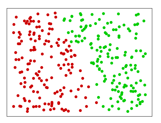
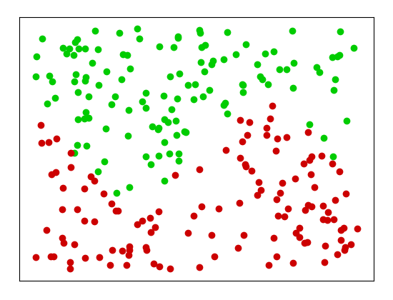
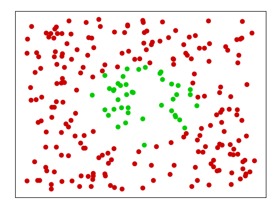
(a)

(b)

(c)

Figure 1: Three 2-class datasets with areas of model uncertainty.

Given the model and one of the uncertainty criteria, we can compute the uncertainty of any point in space. For each dataset, the areas of uncertainty of the model are represented, with more red for more uncertainty. It is remarkable that these uncertainty areas can be compared to the decision boundaries of the model. Often, the closer the observation is to the decision boundary, the less confident the model is about its prediction.

Uncertainty sampling consists of choosing the observation for which the model is least certain of its prediction. This is one of the basis of active learning, however, other methods allow to extract more information about this uncertainty which leads to the decomposition into epistemic and aleatoric uncertainties.

3 On the interest and limits of epistemic and aleatoric uncertainties for active learning

In this section, we introduce additional elements to decompose the uncertainty of the model so it can focus, in active learning, on the observations that will make it rapidly gain in performance.

The uncertainty $\mathcal{U}(x)$ can be separated into two uncertainties [9], one reducible and the other irreducible. The example of Figure 2 shows these two types of uncertainties, on 2(a) the result of a coin toss is uncertain and it is not possible to generate more knowledge to predict that the coin will flip heads or tails, this ignorance is called aleatoric uncertainty. On 2(b) either heads or tails is written in Finnish, it is an uncertainty that can be resolved by learning this language, it is called epistemic uncertainty.

(a) Aleatoric uncertainty

(b) Epistemic uncertainty

Figure 2: Representation of aleatoric and epistemic uncertainties through the tossing of a coin and the word “heads” or “tails” written in Finnish.

Being able to model these two uncertainties can help delimit where it is more interesting to provide knowledge and where it is useless. The total uncertainty $\mathcal{U}(x)$ is often represented as the sum of the epistemic uncertainty $\mathcal{U}_{e}(x)$ and the aleatoric uncertainty $\mathcal{U}_{a}(x)$: $\mathcal{U}(x)=\mathcal{U}_{e}(x)+\mathcal{U}_{a}(x)$.

For a two-class problem $\Omega=\{0,1\}$, it is proposed in [18] to model this uncertainty (here under the [15] formalism) by computing the plausibility $\pi$ of belonging to each of the two classes with the following formula, according to a probabilistic model $\theta$:

$$\begin{split}\pi(1|x)=\underset{\theta\in\Theta}{\text{sup}}\;\text{min}[\pi_{\Theta}(\theta),p_{\theta}(1|x)-p_{\theta}(0|x)],\\ \pi(0|x)=\underset{\theta\in\Theta}{\text{sup}}\;\text{min}[\pi_{\Theta}(\theta),p_{\theta}(0|x)-p_{\theta}(1|x)],\end{split}$$ (6)

with $\pi_{\Theta}(\theta)$ depending on the likelihood $L(\theta)$ and the maximum likelihood $L(\hat{\theta})$:

$$\medmath{\pi_{\Theta}(\theta)=\frac{L(\theta)}{L(\hat{\theta})}.}$$ (7)

The epistemic uncertainty is then high when the two classes are very plausible while the aleatoric uncertainty is high when the two classes are implausible:

$$\begin{split}&\mathcal{U}_{e}(x)=\text{min}[\pi(1|x),\pi(0|x)],\\ &\mathcal{U}_{a}(x)=1-\text{max}[\pi(1|x),\pi(0|x)].\end{split}$$ (8)

This calculation depends not only on the prediction of the model but also on the observations. To summarize, the fewer observations there are in a region, or the fewer decision elements there are to strongly predict a class, the higher the plausibility of the two classes, and the more reducible (and thus epistemic) the uncertainty is by adding knowledge.

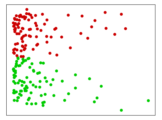
(a) Sample

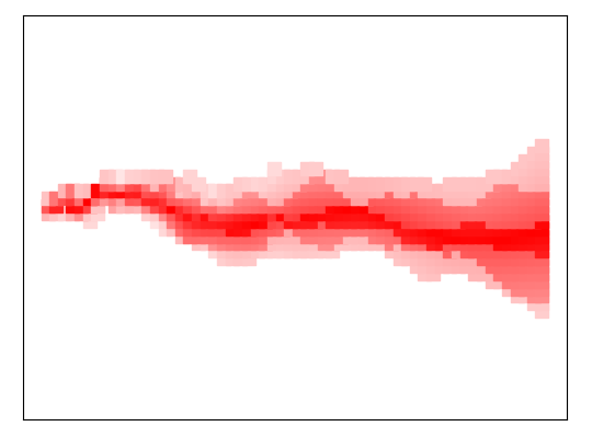
(b) Uncertainty

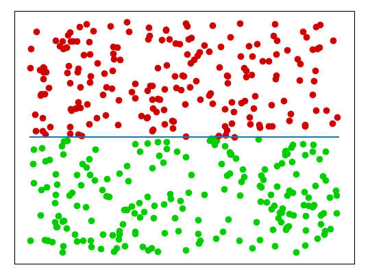
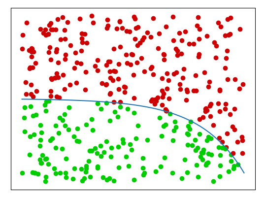
Figure 3: Sample with areas of uncertainty according to the uncertainty sampling and three possible datasets based on the observations available in 3(a).

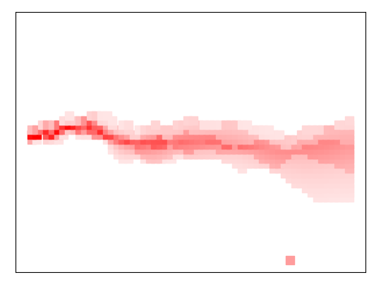
(a) Aleatoric: $\mathcal{U}_{a}$

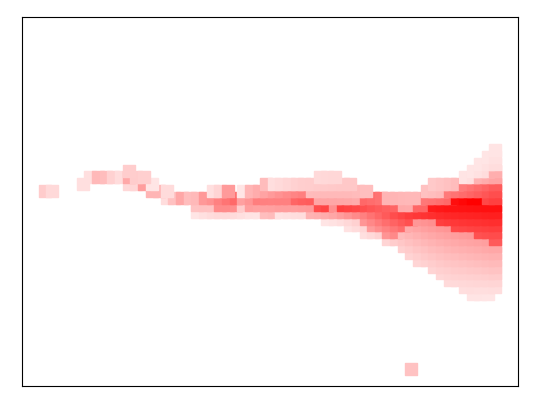
(b) Epistemic: $\mathcal{U}_{e}$

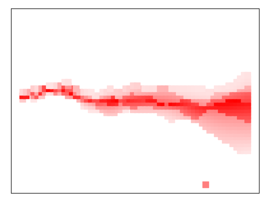
(c) Total: $\mathcal{U}$

Figure 4: Areas of uncertainty on 3(a) for epistemic and aleatoric uncertainties.

An example is shown in Figure 3, a two-class dataset is shown in 3(a) and the areas of model uncertainty are shown in 3(b) according to the uncertainty sampling presented in the previous section. An horizontal line can be distinguished where the model uncertainty is highest. However, the sample represented in 3(a), shows that part of the uncertainty can be removed more easily by adding observations. In the same figure, three different datasets show how the sample can evolve by adding observations. Whatever the final distribution, the uncertainty on the left is not very reducible, while the uncertainty on the right can be modified by adding knowledge.

These two uncertainties can be calculated using equation (8), and are shown in Figure 4. The aleatoric uncertainty, and therefore irreducible, is represented in 4(a) and the epistemic uncertainty, reducible, is represented in 4(b). The total uncertainty is then the sum of the two 4(c). The goal here is to use only the epistemic uncertainty, to know the areas where the model can learn new knowledge and where it will have more impact.

Using epistemic uncertainty as a sampling strategy is not reductive since it provides similar areas of uncertainty to those used previously, where epistemic and aleatoric uncertainty are indistinguishable.

Such information can be useful to find areas of reducible uncertainty, but it is not compatible with richer labels that also contain uncertainty. The way to compute this epistemic uncertainty is also dependent on the observations in addition to the model (i.e. the method could be oversimplified as: the model defines its zones of uncertainty, in which we look for the location with the smallest number of observations to define the reducible uncertainty.). Furthermore, the exploration-exploitation problem is not fully addressed. This leads to the next section in which two uncertainty sampling strategies for rich labels are proposed, they are also extended to several classes.

4 Richer labels and multiple classes

In this section, we propose two uncertainty sampling strategies, with a simplified calculation phase, able to deal with richer labels and no longer directly dependent on the observations but only on the model prediction. We also propose a natural extension for a number of classes higher than two. The first method uses discord and non-specificity to map uncertainty in order to address the exploration-exploitation problem. The second method extends the epistemic and aleatoric uncertainties to rich labels, also simplifying the computation phase.

From there, a label can be uncertain and imprecise, which means that additional information on ignorance is represented. Figure 5 shows how these labels are represented in this document, the darker the dot, the less ignorance the label contains (e.g. I’m sure this is a dog), the lighter the dot, the more ignorance it contains (e.g. I have no idea between dog and cat).

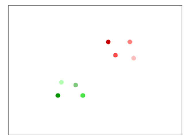
Figure 5: Observations on two dimensions with their rich labels, the darker the point, the more certain and precise its label.

4.1 Discord and non-specificity: Klir uncertainty

In the framework of belief functions, discord and non-specificity are tools that allow to model uncertainty, we propose to use Klir’s representation [12] for uncertainty sampling, some bridges can be made with epistemic and aleatoric uncertainty.

4.1.1 Discord

is here applied to the output of a model capable of making an uncertain and imprecise prediction. It represents the amount of conflicting information in the model’s prediction and is calculated with the following formula:

$$D(m)=-\sum_{A\subseteq\Omega}m(A)\text{ log}_{2}(BetP(A)),$$ (9)

with $m$ a mass function, or the output of the model (see section 2).

Figure 6 represents three different cases where the discord varies, from high discordance where labels around the central point (the observation to label) highly disagree 6(a), to low discordance where each of the labels is in agreement 6(c).

4.1.2 Non-Specificity

allows to quantify the degree of ignorance of the model, the higher it is, the more imprecise the response of the model, it is calculated with:

$$N(m)=\sum_{A\subseteq\Omega}m(A)\text{ log}_{2}(|A|).$$ (10)

The same Figure 6 also represents three different cases of non-specificity, in 6(d) the non-specificity is low as there are relevant sources of information next to the observation to be labelled, in 6(e) the non-specificity increases the further away the elements are from the observation and in 6(f) the non-specificity is also high because the nearby sources of information are themselves ignorant.

(a) High discord

(b) Low discord

(c) No discord

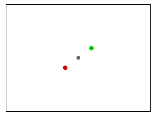
(d) Low non-specificity

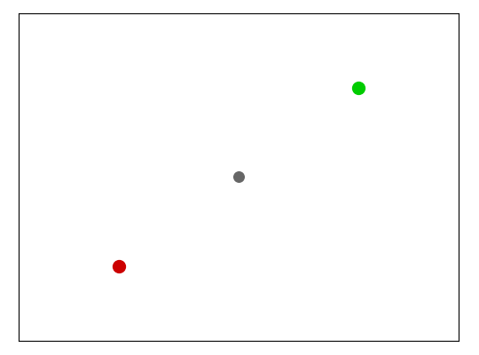
(e) High non-specificity

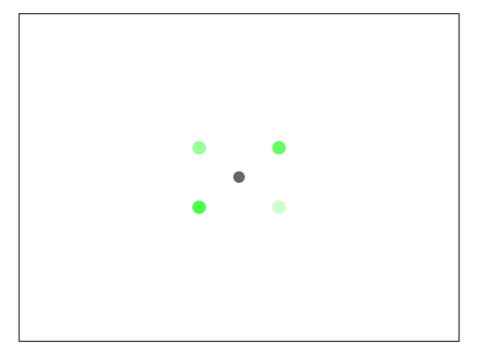
(f) High non-specificity

Figure 6: Three degrees of discord and three degrees of non-specificity in the center.

4.1.3 Klir uncertainty

is then derived from discord and non-specificity, it is used here for uncertainty sampling by adding the two previous formulas:

$$\mathcal{U}_{m}(x)=N(x)+D(x),$$ (11)

with $N(x)$ and $D(x)$ respectively the non-specificity and discord of the model in $x$. Klir [12] proposes to use the same weight for discord and non-specificity, but in [4] a parameter $\lambda\in[0,1]$ is introduced and allows to bring more weight to non-specificity (we propose to use it for more exploration) or to discord (for more exploitation):

$$\mathcal{U}_{m}(x)=\lambda N(x)+(1-\lambda)D(x).$$ (12)

Note that this uncertainty is naturally extended to $|\Omega|\geq 2$ classes.

This formula has the advantage of identifying the total uncertainty as well as the reducible one, but also of taking into account the uncertainty already present in the labels and of being adjustable for more exploration or exploitation. Figure 7 shows a dataset with two areas of uncertainty 7(a), on the right an area with a lack of data and on the left an area where labels are more ignorant. The uncertainty sampling, using Shannon’s entropy (4) or the least confidence measure (5) is not able to see either of these two areas 7(b). The epistemic uncertainty (8) is able to distinguish the uncertainty related to the arrangement of the observations in space (i.e. the uncertainty on the right) but not the uncertainty related to the ignorance of the sources 7(c).

(a) Dataset

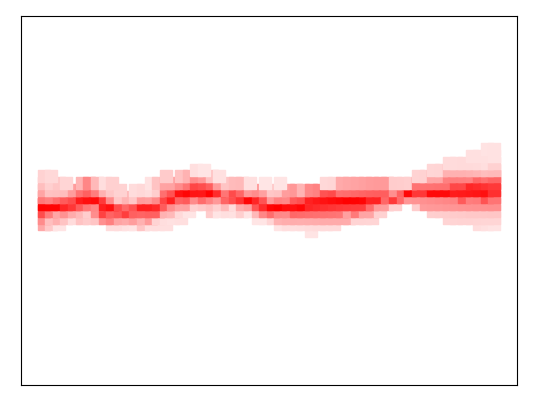
(b) Uncertainty

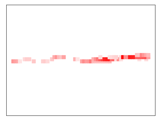
(c) Epistemic

Figure 7: An imperfectly labeled dataset 7(a) with the areas of uncertainty according to uncertainty sampling and epistemic uncertainty.

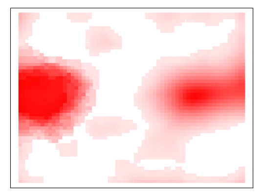
(a) Non-specificity

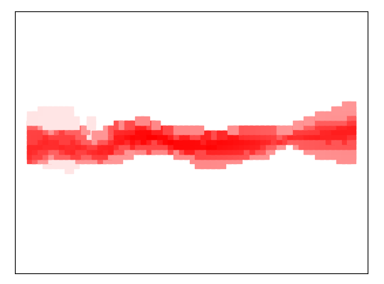
(b) Discord

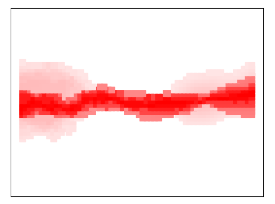
(c) Klir

Figure 8: Areas of uncertainty corresponding to the dataset 7(a) according to the non-specificity, the discord and the total uncertainty defined by Klir.

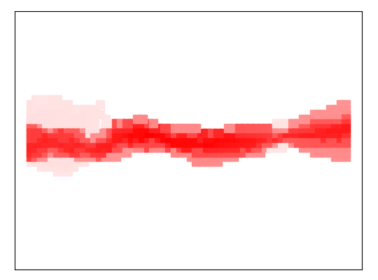
(a) More exploitation

(b) Compromise

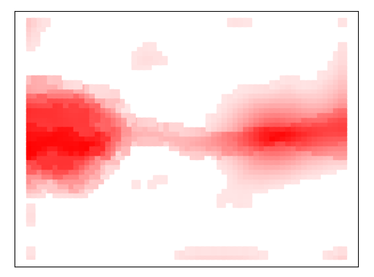
(c) More exploration

Figure 9: Areas of Klir uncertainty, modifying the amount of non-specificity and discord. With $\lambda=0.1$, more discord is taken into account, with $\lambda=0.5$, discord and non-specificity are used as much and with $\lambda=0.9$, more non-specificity is taken into account.

The proposal of using Klir uncertainty for sampling (discord and non-specificity) allows to represent each of these uncertainties. Figure 8 shows the areas of non-specificity 8(a), of discord 8(b) and Klir uncertainty 8(c).

Klir uncertainty can then be used for uncertainty sampling in active learning, it is also possible to vary the result for more exploration or more exploitation by modifying $\lambda$. Figure 9 shows the areas of uncertainty for different values of $\lambda$, more discord on the left to more non-specificity on the right.

We have proposed here to use Klir’s uncertainty in sampling, which allows to represent some unknown uncertainties areas in active learning related to rich labels. The method is no longer dependent on the observations, but only on the prediction of the model and the exploration-exploitation problem is addressed thanks to the $\lambda$ parameter. Even though discord may recall aleatoric uncertainty (non-reducible) and non-specificity may recall epistemic uncertainty (reducible). These notions are not quite equivalent. Therefore, in the following section we also propose an extension of epistemic (and aleatoric) uncertainty for rich labels and for several classes.

4.2 Evidential epistemic uncertainty

We propose here to extend the notion of epistemic uncertainty to rich labels, by removing the dependence on observations, simplifying the computational phase, and allowing the model to detect new areas of uncertainty.

The epistemic uncertainty can be extended to rich labels by using the notion of plausibility within the framework of belief functions. It represents the total evidence that does not support the complementary event for a class $\omega$ or more generally for an element $A\in 2^{\Omega}$. The plausibility $Pl$ defines the belief that could be allocated to $A$:

$$Pl(A)=\sum_{A\cap B\neq\emptyset}m(B).$$ (13)

The plausibility being the consistent evidence, the belief function $Bel$ defines the total evidence directly supporting $A$:

$$Bel(A)=\sum_{B\subseteq A,B\neq\emptyset}m(B).$$ (14)

We have $Pl(A)=1-Bel(\bar{A})$. Analogous to equation (8) and for two classes $\Omega=\{0,1\}$ the epistemic uncertainty is maximal when both classes are highly plausible. The proposed evidential epistemic and aleatoric uncertainties are defined as follows:

$$\begin{split}&\mathcal{U}_{e}(x)=\text{min}[Pl(1|x),Pl(0|x)],\\ &\mathcal{U}_{a}(x)=1-\text{max}[Pl(1|x),Pl(0|x)].\end{split}$$ (15)

The equation for the aleatoric uncertainty can be rewritten depending on the belief $Bel$:

$$\mathcal{U}_{a}(x)=\text{min}[Bel(1|x),Bel(0|x)].\\$$ (16)

The sum of the epistemic and aleatoric uncertainties is then the total evidential uncertainty: $\mathcal{U}(x)=\mathcal{U}_{e}(x)+\mathcal{U}_{a}(x)$. However, when the number of classes exceeds 2 the equation of the epistemic uncertainty cannot be simplified by the minimum plausibility:

$$\begin{split}&\mathcal{U}_{e}(x)\neq\text{min}([Pl(\omega|x)|\omega\in\Omega]),\\ &\mathcal{U}_{a}(x)\neq 1-\text{max}([Pl(\omega|x)|\omega\in\Omega]).\end{split}$$ (17)

It is preferable to first define the uncertainty related to one of the classes $\omega$, rewritten with the belief $Bel$ to avoid having to manipulate $\bar{\omega}$:

$$\begin{split}\mathcal{U}_{e}(\omega|x)&=\text{min}[Pl(\omega|x),Pl(\bar{\omega}|x)]\\ &=\text{min}[Pl(\omega|x),1-Bel(\omega|x)].\end{split}$$ (18)

The evidential extension of the epistemic and aleatoric uncertainties for $|\Omega|\geq 2$ classes is then:

$$\begin{split}&\mathcal{U}_{e}(x)=\sum_{\omega\in\Omega}\text{min}[Pl(\omega|x),1-Bel(\omega|x)],\\ &\mathcal{U}_{a}(x)=\sum_{\omega\in\Omega}\text{min}[Bel(\omega|x),1-Pl(\omega|x)].\end{split}$$ (19)

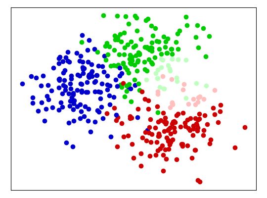
(a) Dataset

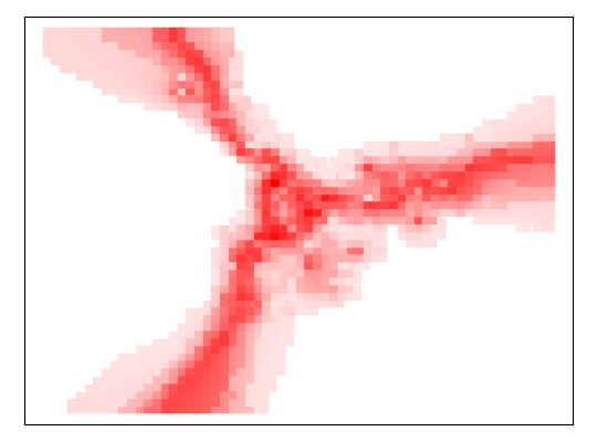
(b) Uncertainty

Figure 10: On the left, a sample of a dataset of three classes with an area of ignorance (labeled with imprecision) and on the right areas of uncertainty according to non-evidential uncertainty sampling.

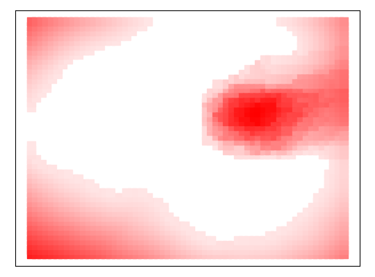
(a) Non-specificity

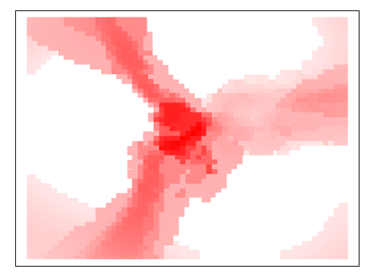
(b) Discord

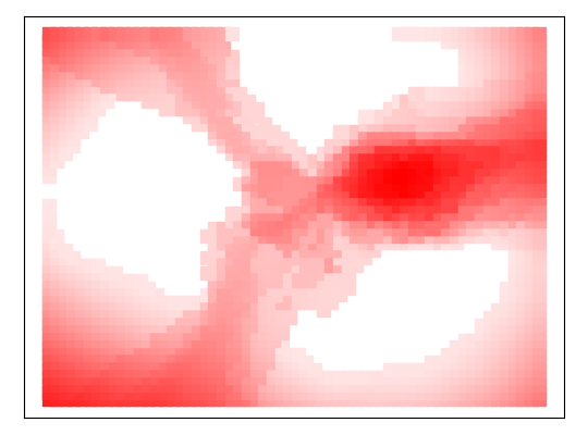
(c) Klir

Figure 11: Areas of uncertainty corresponding to the datasets 10(a) according to the non-specificity, the discord and the total Klir uncertainty.

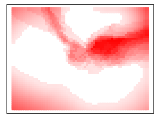
(a) Green class

(b) Red class

(c) Blue class

Figure 12: Areas of uncertainty corresponding to the datasets 10(a) according to the evidential epistemic uncertainty for green, red and blue classes.

(a) Evidential aleatoric

(b) Evidential epistemic

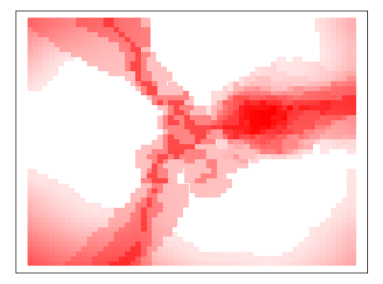
(c) Evidential total

Figure 13: Areas of uncertainty for evidential epistemic and aleatoric uncertainties, according to 10(a).

The example in Figure 10 shows a dataset of three classes with a zone of ignorance for some labels (between the green and red classes). Probabilistic (4)-(5) and epistemic (8) uncertainties cannot model the imprecision present in the labels, this less complete uncertainty zone is represented in 10(b).

The previous uncertainty resulting from the sum of the discord and the non-specificity is presented in Figure 11. It manages both exploration 11(a) and exploitation 11(b) to give a better representation of the uncertainty 11(c).

The extension of the epistemic uncertainty, also introduced in this paper, is presented in the following experiments. First, the evidential epistemic areas of uncertainties for each of the three classes are presented in Figure 12. Then, the resulting evidential epistemic uncertainty of the model is deducted from equation (19) in Figure 13 along with the evidential aleatoric and total uncertainties.

5 Sampling on real world dataset

Some datasets have been labeled in an uncertain and imprecise way by users during crowdsourcing campaigns [22]. We therefore have access to really imperfectly labeled datasets with rich labels. Conventional methods for computing model uncertainty do not take into account the degrees of imprecision of these rich labels. The two proposed methods are illustrated on Credal Dog-2, one of these datasets. Figure 14 shows the dataset on the two first components of a Principal Component Analysis. This is a two-class dataset represented in 14(a) with true classes and in 14(b) with uncertain and imprecise rich labels given by contributors. Darker dots indicate higher certainty, and vice versa.

Figure 16 shows the result of the first proposed method, sampling by Klir uncertainty, on the dataset with rich labels. The non-specificity is presented 15(a) and can be interpreted as the ignorance zones of the model. Discord is also represented 15(b) and the total uncertainty 15(c) is the sum of the two, it is this latter information that is used to sample on the model uncertainty.

The second proposed method, the extension of epistemic uncertainty, which is a reducible uncertainty applied to evidential reasoning, is presented in Figure 16. The irreducible aleatoric evidential uncertainty 16(a) is presented along with the reducible epistemic evidential uncertainty 16(b). The total uncertainty 16(c) is the sum of the reducible and irreducible uncertainties. For active learning, it is not the total uncertainty, but the epistemic reducible uncertainty that is used.

6 Discussion & Conclusion

The calculation of epistemic uncertainty (non-evidential) is demanding, and not necessarily accessible. It is, depending on the observations, necessary to go through several phases of computation, estimation of likelihood, maximum likelihood and optimization.

In this paper, we have proposed two new uncertainty sampling strategies and a new way to represent them. With these two proposed methods, the use of Klir uncertainty and the extended evidential epistemic uncertainty, a simple calculation on the output of the model allows to obtain the uncertainties. The objective is to also take into account the uncertainty present in richer labels, which is currently not possible. The first strategy is based on Klir’s uncertainty, combining discord (how self-conflicting the information is) and non-specificity (how ignorant the information is) in the model output. The second strategy extends epistemic (reducible) uncertainty to the evidential framework and to several classes, simplifying the computational phase.

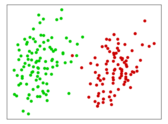
(a) True labels

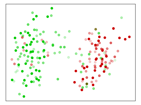
(b) Rich labels

Figure 14: Credal Dog-2 dataset, Brittany breed is in green and Beagle in red.

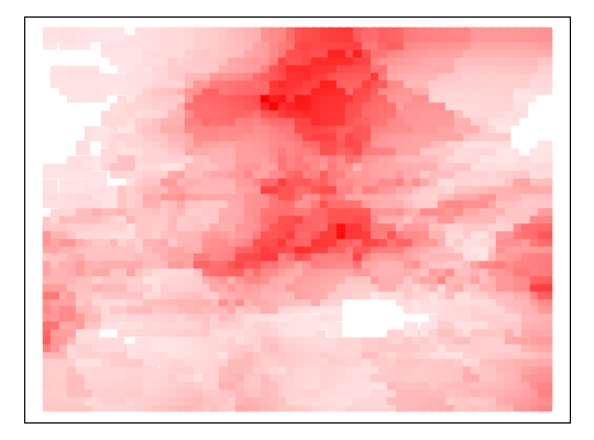
(a) Non-specificity

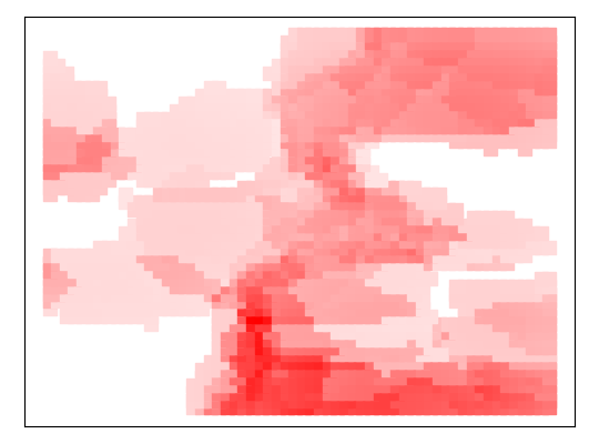
(b) Discord

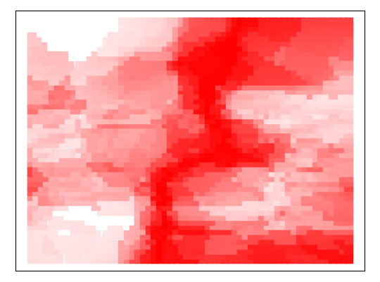
(c) Klir

Figure 15: Areas of uncertainty corresponding to the dataset 14(b) according to the non-specificity, the discord and to the total Klir uncertainty.

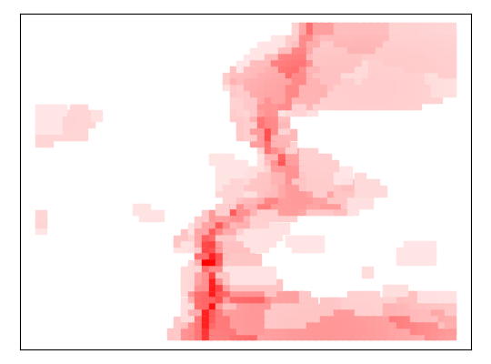
(a) Evidential aleatoric

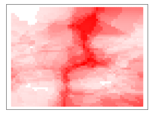
(b) Evidential epistemic

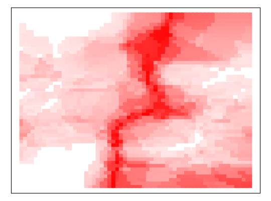
(c) Evidential total

Figure 16: Areas of evidential epistemic uncertainty corresponding to 14(b).

This simplicity obviously has a counterpart: the model must be able to deliver a mass function, to represent uncertainty and imprecision in the output. Such models exist but are not numerous, among them are the much quoted Evidential $K$-Nearest Neighbors [5], Evidential Decision Trees [6, 4], Evidential Random Forest and even Evidential Neural Networks [23]. The proposed methods are compatible with probabilistic models (since a probability is a special mass function) but the full depth of evidence modeling would be lost.

The novelty of this work lies in the representation of new information for uncertainty sampling, rather than in performance comparison. The next step is to apply these models to active learning, where the learning model has access to a very limited number of labeled observations, and must choose the most relevant observations to label in order to increase performance. The ability of the model to define these areas of uncertainty, and to categorize these uncertainties, is then relevant information.

Supplementary materials

Reproducibility

This section deals with the experiments presented in this document, with the different parameters for each experiment. Note that every datasets as well as the code in Python allowing to reproduce these experiments are available at: https://anonymous.4open.science/r/evidential-uncertainty-sampling-D453.

Uncertainty sampling

The three datasets

are generated according to the following separation line:

1. $y=-3x$

2. $y=\text{sin}(0.8x)$

3. $(x-0)^{2}+(y-0)^{2}=6$

The uncertainties

are computed on a grid of $60*50$ points (it is the same for every experiments). The used model is $K$-NN ($K$-Nearest Neighbors), with a probabilistic output and on the distance-weighted version available with scikit-learn [16] (every other parameters are the scikit-learn default parameters). The model is trained on the dataset and then try to predict the class of every data point of the grid by using 10 nearest neighbors. The uncertainty used is the least confidence measure given in equation (5) and the same parameters are used on Fisher’s Iris dataset.

6.0.1 Example on real world dataset:

An example on real data is presented in Figure 17, Fisher’s Iris dataset is presented on two variables. The three Iris classes are shown in 17(a) and the areas of model uncertainty are shown in 17(b), these are the regions where the model would be the most uncertain to predict the class of a new observation. This is summarized by the fact that if a new observation falls into a red zone, the model will have more difficulty predicting its class.

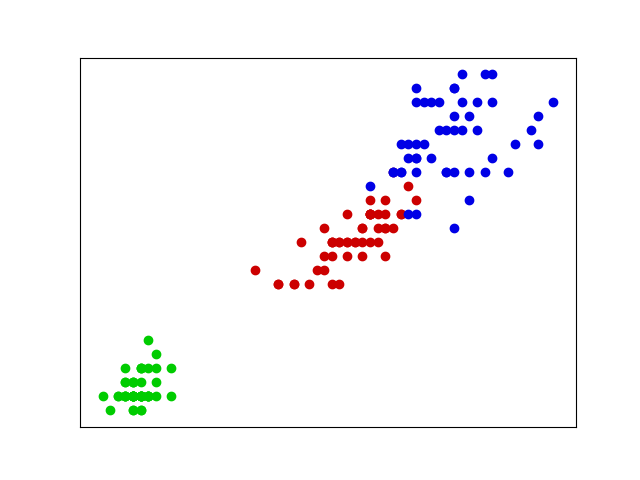
(a) Iris Dataset

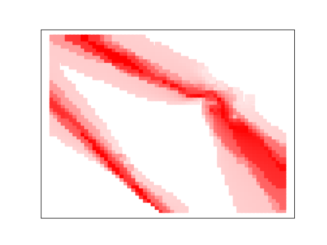
(b) Uncertainty

Figure 17: Fisher’s Iris dataset on two descriptive variables, petal length and width, with model uncertainties. Setosa in green, Versicolor in red and Virginica in blue.

Epistemic and aleatoric uncertainties

The dataset

is generated according to the separation line of equation $y=0$ and the data points are generated, with more points on the left according to a binary logarithm $\text{log}_{2}$.

The uncertainties

are computed according to the same version of the $K$-Nearest Neighbors algorithm. The experimental process follows the one described in [15]. The formulas are deduced from equation (6) as follows:

$$\begin{split}&\pi(1|x)=\underset{\theta\in\Theta}{\text{sup}}\;\text{min}[\pi_{\Theta}(\theta),p_{\theta}(1|x)-p_{\theta}(0|x)],\\ &\pi(0|x)=\underset{\theta\in\Theta}{\text{sup}}\;\text{min}[\pi_{\Theta}(\theta),p_{\theta}(0|x)-p_{\theta}(1|x)].\end{split}$$ (20)

That can be rewritten with $f(a)=2a-1$:

$$\begin{split}&\pi(1|x)=\underset{\theta\in\Theta}{\text{sup}}\;\text{min}[\pi_{\Theta}(\theta),f(p_{\theta}(1|x))],\\ &\pi(0|x)=\underset{\theta\in\Theta}{\text{sup}}\;\text{min}[\pi_{\Theta}(\theta),f(1-p_{\theta}(1|x))],\end{split}$$ (21)

with:

$$\pi_{\Theta}(\theta)=\frac{L(\theta)}{L(\hat{\theta})},$$ (22)

For a Parzen window, as described in [15] and with $p$ and $n$ the number of positive and negative instances within the window, $L(\theta)$ is:

$$L(\theta)=\binom{p+n}{p}\theta^{p}(1-\theta)^{n},\;\text{and}\;\;\hat{\theta}=\frac{p}{p+n}$$ (23)

As we are not using a Parzen window but the distance-weighted $K$-NN, we take $p$ the sum of the inverse distance for positive elements among the $K$ neighbors, and $n$ reciprocally the same for the negative class. Yet we have:

$$\begin{split}&\pi(1|x)=\underset{\theta\in[0,1]}{\text{sup}}\;\text{min}\left(\frac{\theta^{p}(1-\theta)^{n}}{\left(\frac{p}{p+n}\right)^{p}\left(\frac{n}{p+n}\right)^{n}},2\theta-1\right),\\ &\pi(0|x)=\underset{\theta\in[0,1]}{\text{sup}}\;\text{min}\left(\frac{\theta^{p}(1-\theta)^{n}}{\left(\frac{p}{p+n}\right)^{p}\left(\frac{n}{p+n}\right)^{n}},1-2\theta\right).\end{split}$$ (24)

Brent’s method is applied to find a local minimum (here the maximum) in the interval $\theta\in[0,1]$. Note that in this paper, the experimental results are not there to compare a performance gap, but to support a new approach to sampling by uncertainty. And, in our case, we have deduced the following formula more appropriate, so it is this one that we use in the presented experiments:

$$\begin{split}&\pi(1|x)=\underset{\theta\in[0,1]}{\text{sup}}\;\text{min}\left(\frac{\theta^{p}(1-\theta)^{n}}{\left(\frac{p}{p+n}\right)^{p}\left(\frac{n}{p+n}\right)^{n}},2\theta-1\right),\\ &\pi(0|x)=1-\underset{\theta\in[0,1]}{\text{sup}}\;\text{min}\left(\frac{\theta^{p}(1-\theta)^{n}}{\left(\frac{p}{p+n}\right)^{p}\left(\frac{n}{p+n}\right)^{n}},1-2\theta\right),\end{split}$$ (25)

and for the uncertainties:

$$\begin{split}&\mathcal{U}_{e}(x)=\text{min}[\pi(1|x),\pi(0|x)]-0.5,\\ &\mathcal{U}_{a}(x)=1-\text{max}[\pi(1|x),\pi(0|x)].\end{split}$$ (26)

The computational complexity, the dependence on observations, the optimization phase, the use of likelihood and maximum likelihood make the model heavier. In the next two experiments and thus for the proposed models, a simple output-dependent calculation replaces all these steps.

Discord and non-specificity

The dataset

is generated according to the separation line of equation $y=0$ and the data points are added, with no observations in the subspace verifying $(x-2.8)^{2}+(y-0)^{2}<5$ and with imprecise (or more ignorant) observations in the subspace verifying $(x-4.5)^{2}+(y-0)^{2}<5$.

The evidential uncertainties

are computed according to the Evidential $K$-Nearest Neighbors algorithm [5]. The parameters are those used in the $\gamma$-E$K$-NN version presented in [8], with $K=10$ nearest neighbors, $\beta=2$, $\alpha=1$ and the formula (12) is used with $\lambda=0.5$, as suggested in [12]. When $\lambda$ varies the values taken are $\lambda=0.1$ and $\lambda=0.9$. A difference is made with respect to the Evidential $K$-Nearest Neighbors model, instead of the conjunctive combination of Demster, a combination by average of the masses (3) is used (which allows to pass $\alpha$ to 1, instead of $\alpha<1$).

Evidential epistemic uncertainty

The dataset

is generated according to three gaussian scikit-learn blobs [16] with imprecise (or more ignorant) observations in the subspace verifying $(2.3-x)^{2}+(3-y)^{2}<2$.

The evidential epistemic uncertainty

is computed according to the same Evidential $K$-Nearest Neighbors with $K=6$ nearest neighbors, $\beta=2$, $\alpha=1$ and the formula (19) is used to compute both the proposed evidential epistemic and aleatoric uncertainties.

Non-regression for advanced methods

This section shows that for the models presented, whether epistemic uncertainty or the proposition to use Klir uncertainty and evidential epistemic uncertainty, none is reductive regarding the (4) and (5) classical measures. Effectively it offers similar areas of uncertainty as the one used is section 2 when epistemic, aleatoric and evidential uncertainties are indistinguishable. Figures 18, 19 and 20 show the areas of uncertainty on the datasets introduced in Figure 1. The epistemic uncertainty, Klir uncertainty and the evidential epistemic uncertainty offers, roughly, the same areas of uncertainty as the one used in Figure 1.

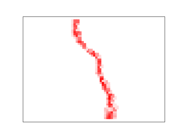
(a)

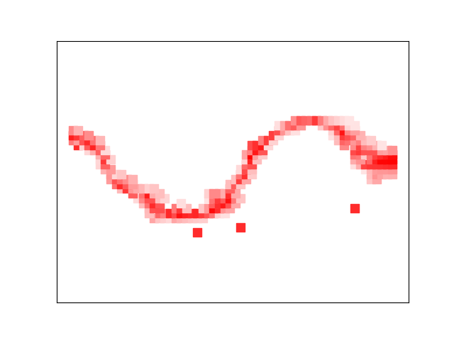
(b)

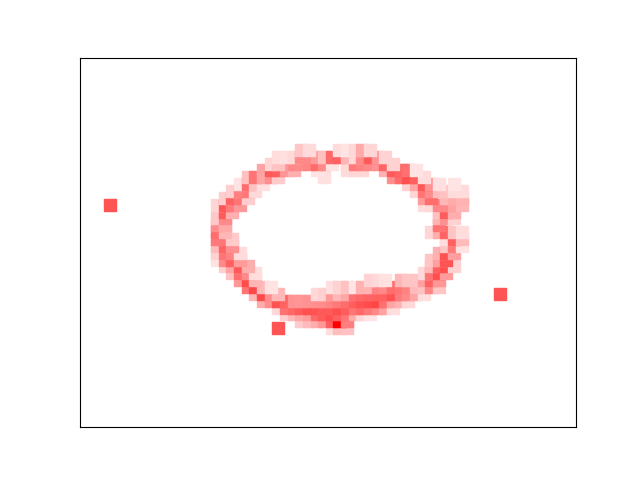
(c)

Figure 18: From left to right, the areas of uncertainty corresponding to the datasets 1(a), 1(b) and 1(c) according to the epistemic uncertainty.

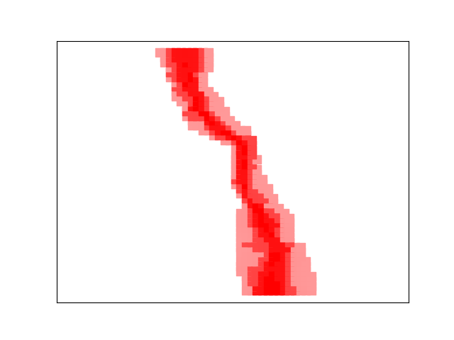
(a)

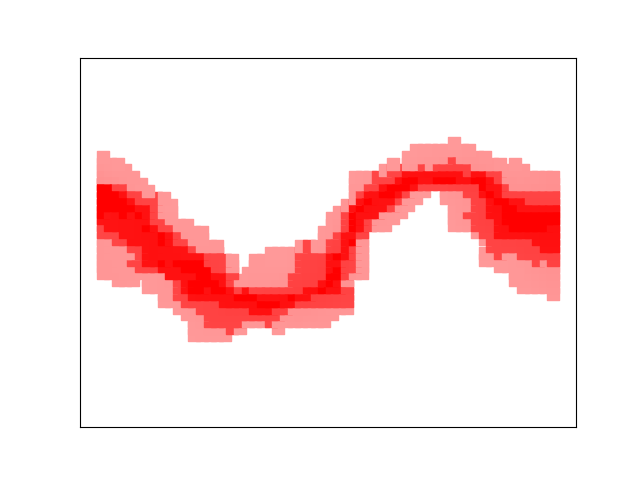
(b)

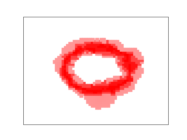
(c)

Figure 19: From left to right, the areas of uncertainty corresponding to the datasets 1(a), 1(b) and 1(c) according to Klir uncertainty resulting from the discord and the non-specificity.

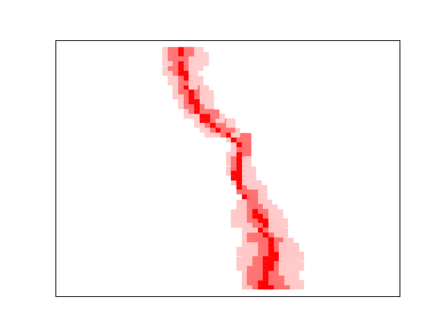
(a)

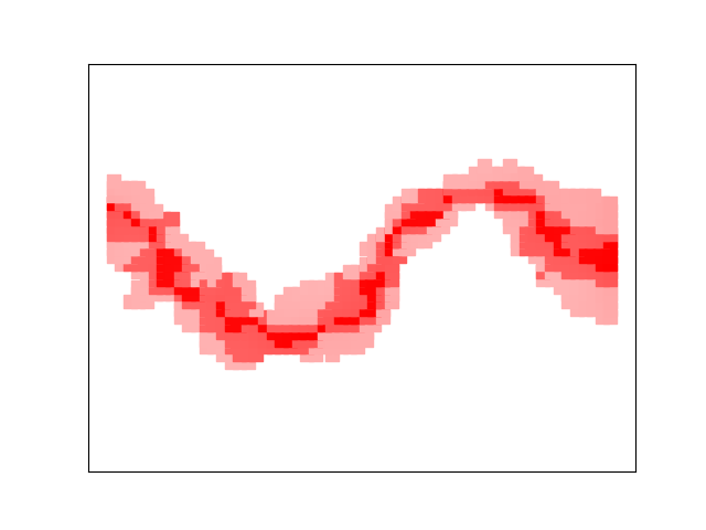
(b)

(c)

Figure 20: From left to right, the areas of uncertainty corresponding to the datasets 1(a), 1(b) and 1(c) according to the evidential epistemic uncertainty.

References

- [1] Aggarwal, C., Kong, X., Gu, Q., Han, J., Yu, P.: Active Learning: A Survey, Data Classification: Algorithms and Applications. CRC Press (2014)
- [2] Bondu, A., Lemaire, V., Boullé, M.: Exploration vs. exploitation in active learning: A bayesian approach. In: The 2010 International Joint Conference on Neural Networks (IJCNN). pp. 1–7 (2010)
- [3] Dempster, A.P.: Upper and Lower Probabilities Induced by a Multivalued Mapping. The Annals of Mathematical Statistics 38(2), 325 – 339 (1967)
- [4] Denoeux, T., Bjanger, M.: Induction of decision trees from partially classified data using belief functions. Systems, Man, and Cybernetics, 2000 IEEE International Conference 4, 2923–2928 (2000)
- [5] Denœux, T.: A k-nearest neighbor classification rule based on dempster-shafer theory. Systems, Man and Cybernetics, IEEE Transactions on 219 (1995)
- [6] Elouedi, Z., Mellouli, K., Smets, P.: Belief decision trees: theoretical foundations. International Journal of Approximate Reasoning 28(2), 91–124 (2001)
- [7] Fredriksson, T., Mattos, D.I., Bosch, J., Olsson, H.H.: Data labeling: An empirical investigation into industrial challenges and mitigation strategies. In: Morisio, M., Torchiano, M., Jedlitschka, A. (eds.) Product-Focused Software Process Improvement. pp. 202–216. Springer International Publishing, Cham (2020)
- [8] Hoarau, A., Martin, A., Dubois, J.C., Le Gall, Y.: Imperfect labels with belief functions for active learning. In: Belief Functions: Theory and Applications. Springer International Publishing (2022)
- [9] Hora, S.C.: Aleatory and epistemic uncertainty in probability elicitation with an example from hazardous waste management. Reliability Engineering & System Safety 54(2), 217–223 (1996), treatment of Aleatory and Epistemic Uncertainty
- [10] Hüllermeier, E., Waegeman, W.: Aleatoric and epistemic uncertainty in machine learning: An introduction to concepts and methods. Machine Learning 110, 457–506 (2021)
- [11] Kendall, A., Gal, Y.: What uncertainties do we need in bayesian deep learning for computer vision? In: NIPS (2017)
- [12] Klir, G.J., Wierman, M.J.: Uncertainty-based information: Elements of generalized information theory. In: Springer-Verlag (1998)
- [13] Lewis, D.D., Gale, W.A.: A sequential algorithm for training text classifiers. In: SIGIR (1994)
- [14] Martin, A.: Conflict management in information fusion with belief functions. In: Bossé, E., Rogova, G.L. (eds.) Information quality in information fusion and decision making, pp. 79–97. Information Fusion and Data Science, Springer (2019)
- [15] Nguyen, V.L., Shaker, M.H., Hüllermeier, E.: How to measure uncertainty in uncertainty sampling for active learning. Mach. Learn. 111, 89–122 (jan 2022)
- [16] Pedregosa, F., Varoquaux, G., Gramfort, A., Michel, V., Thirion, B., Grisel, O., Blondel, M., Prettenhofer, P., Weiss, R., Dubourg, V., Vanderplas, J., Passos, A., Cournapeau, D., Brucher, M., Perrot, M., Duchesnay, E.: Scikit-learn: Machine learning in Python. Journal of Machine Learning Research 12, 2825–2830 (2011)
- [17] Roh, Y., Heo, G., Whang, S.E.: A survey on data collection for machine learning: A big data - ai integration perspective. IEEE Transactions on Knowledge and Data Engineering 33(4), 1328–1347 (2021)
- [18] Senge, R., Bösner, S., Dembczynski, K., Haasenritter, J., Hirsch, O., Donner‐Banzhoff, N., Hüllermeier, E.: Reliable classification: Learning classifiers that distinguish aleatoric and epistemic uncertainty. Inf. Sci. 255, 16–29 (2014)
- [19] Settles, B.: Active learning literature survey. Computer Sciences Technical Report 1648, University of Wisconsin–Madison (2009)
- [20] Shafer, G.: A Mathematical Theory of Evidence. Princeton University Press, Princeton (1976)
- [21] Smets, P., Kennes, R.: The transferable belief model. Artificial Intelligence 66(2), 191–234 (1994)
- [22] Thierry, C., Hoarau, A., Martin, A., Dubois, J.C., Le Gall, Y.: Real bird dataset with imprecise and uncertain values. In: 7th International Conference on Belief Functions (2022)
- [23] Yuan, B., Yue, X., Lv, Y., Denoeux, T.: Evidential Deep Neural Networks for Uncertain Data Classification. In: Knowledge Science, Engineering and Management (Proceedings of KSEM 2020). Lecture Notes in Computer Science, Springer Verlag (Aug 2020)