Technical Report: Differentially Private Reward Functions
for Markov Decision Processes

Abstract

Markov decision processes often seek to maximize a reward function, but onlookers may infer reward functions by observing agents, which can reveal sensitive information. Therefore, in this paper we introduce and compare two methods for privatizing reward functions in policy synthesis for multi-agent Markov decision processes, which generalize Markov decision processes. Reward functions are privatized using differential privacy, a statistical framework for protecting sensitive data. The methods we develop perturb (i) each agent’s individual reward function or (ii) the joint reward function shared by all agents. We prove that both of these methods are differentially private and show approach (i) provides better performance. We then develop an algorithm for the numerical computation of the performance loss due to privacy on a case-by-case basis. We also exactly compute the computational complexity of this algorithm in terms of system parameters and show that it is inherently tractable. Numerical simulations are performed on a gridworld example and in waypoint guidance of an autonomous vehicle, and both examples show that privacy induces only negligible performance losses in practice.

I Introduction

Many autonomous systems share sensitive information to operate, such as teams of robots. As a result, there has arisen interest in privatizing such information when it is communicated. However, these protections can be difficult to provide in systems in which agents are inherently observable, such as in a traffic system in which agents are visible to other vehicles [1] or a power system in which power usage is visible to a utility company [2]. These systems do not offer the opportunity to modify communications to protect information precisely because agents are observed directly. A fundamental challenge is that information about agents is visible to observers, though we would still like to limit the inferences that can be drawn from that information.

In this paper, we consider the problem of protecting the reward function of a Markov decision process, even when its states and actions can be observed. In particular, we model individual agents as Markov Decision Processes (MDPs), and we model collections of agents as Multi-Agent Markov Decision Processes (MMDPs). Given that an MDP is simply an MMDP with a single agent, we focus on MMDPs. In MMDPs, agents’ goal is to synthesize a reward-maximizing policy. Accordingly, we develop a method for synthesizing policies that preserve the privacy of the agents’ reward function while still approximately maximizing it.

Since these agents can be observed, the actions they take could reveal their reward function or some of its properties, which may be sensitive information. For example, quantitative methods can draw such inferences from agents’ trajectories both offline [3, 4] and online [5]. Additionally onlookers may draw qualitative inferences from agents as well, such as their goal state [6]. This past work shows that harmful quantitative and qualitative inferences can be drawn without needing to recover the entire reward function. Therefore, we seek to protect agents’ reward functions from both existing privacy attacks and those yet to be developed.

We use differential privacy to provide these protections. Differential privacy is a statistical notion of privacy originally used to protect entries of databases [7]. Differential privacy has been used recently in control systems and filtering [8, 9, 10, 11, 12], and to privatize objective functions in distributed optimization [13, 14, 15, 16, 17, 18]. The literature on distributed optimization has already established that agents’ objective functions require privacy, and a key focus has been convex minimization problems. In this paper, we consider agents maximizing reward functions and hence are different from that work, though the need to protect individual agents’ rewards is just as essential as the protection of objectives in those works.

Differential privacy is appealing because of its strong protections for data and its immunity to post-processing [19]. That is, the outputs of arbitrary computations on differentially private data are still protected by differential privacy. This property provides protections against observers that make inferences about agents’ rewards, including through techniques that do not exist yet. We therefore first privatize reward functions, then using dynamic programming to synthesize a policy with the privatized reward function. Since this dynamic programming stage is post-processing on privatized reward functions, the resulting policy preserves the privacy of the reward functions as well, as do observations of an agent executing that policy and any downstream inferences that rely on those observations.

Of course, we expect perturbations to reward functions to affect performance. To assess the impact of privacy on the agents’ performance we quantify the sub-optimality of the policy synthesized with the privatized reward function. In particular, it relates the total discounted reward (known as the value function) with privacy to that without privacy. We develop an algorithm to compute the cost of privacy, and we compute the exact computational complexity of this algorithm in terms of system parameters. These calculations and simulations both show the tractability of this algorithm.

To summarize, we make the following contributions:

• We develop two differential privacy mechanisms for reward functions in MMDPs. (Theorems 1 and 2)

• We provide an analytical bound on the accuracy of privatized reward functions and use that bound to trade-off privacy and accuracy. (Theorem 3)

• We provide an algorithm to compute the trade-off between privacy and performance, then quantify its computational complexity. (Theorem 4)

• We validate the impact of privacy upon performance in two classes of simulations.

Related Work

Privacy has previously been considered for Markov decision processes, both in planning [20, 21, 22] and reinforcement learning [23, 24]. Privacy has also been considered for Markov chains [25] and for general symbolic systems [26]. The closest work to ours is in [20] and [27]. In [20], privacy is applied to transition probabilities, while we apply it to reward functions. In [27], the authors use differential privacy to protect rewards that are learned. We differ since we consider planning problems with a known reward.

This paper is organized as follows: Section II provides background and problem statements, and Section III presents two methods for privatizing reward functions. Then, Section IV formalizes accuracy-privacy trade-offs, and Section V presents a method of computing the cost of privacy. Section VI provides simulations, and Section VII concludes.

Notation

For $N\in\mathbb{N}$, we use $[N]$ to denote $\{1,2,\ldots,N\}$, we use $\Delta(B)$ to be the set of probability distributions over a finite set $B$, and we use $|\cdot|$ for the cardinality of a set. Additionally, we use $\lceil\cdot\rceil$ as the ceiling function. We use $\pi$ both as the usual constant and as a policy for an MDP since both uses are standard. The meaning will be clear from context.

II Preliminaries and Problem Formulation

This section reviews Markov decision processes and differential privacy, then provides formal problem statements.

II-A Markov Decision Processes

Consider a collection of $N$ agents indexed over $i\in[N]$. We model agent $i$ as a Markov decision process.

Definition 1 (Markov Decision Process).

Agent $i$’s Markov Decision Process (MDP) is the tuple $\mathcal{M}^{i}=(\mathcal{S}^{i},\mathcal{A}^{i},r^{i},\mathcal{T}^{i})$, where $\mathcal{S}^{i}$ and $\mathcal{A}^{i}$ are agent $i$’s finite sets of local states and actions, respectively. Additionally, let $\mathcal{S}=\mathcal{S}^{1}\times\cdots\times\mathcal{S}^{N}$ be the joint state space of all agents. Then $r^{i}:\mathcal{S}\times\mathcal{A}^{i}\rightarrow\mathbb{R}$ is agent $i$’s reward function, and $\mathcal{T}^{i}:\mathcal{S}^{i}\times\mathcal{A}^{i}\rightarrow\Delta(\mathcal{S}^{i})$ is agent $i$’s transition probability function. $\lozenge$

With $\mathcal{T}^{i}:\mathcal{S}^{i}\times\mathcal{A}^{i}\rightarrow\Delta(\mathcal{S}^{i})$, we see that $\mathcal{T}^{i}(s^{i},a^{i})\in\Delta(\mathcal{S}^{i})$ is a probability distribution over the possible next states when taking action $a^{i}\in\mathcal{A}^{i}$ in state $s^{i}\in\mathcal{S}^{i}$. We abuse notation and let $\mathcal{T}^{i}(s^{i},a^{i},y^{i})$ be the probability of transitioning from state $s^{i}$ to state $y^{i}\in\mathcal{S}^{i}$ when agent $i$ takes action $a^{i}\in\mathcal{A}^{i}$. We now model the collection of agents as a Multi-Agent Markov Decision Process (MMDP).

Definition 2 (Multi-Agent Markov Decision Process [28]).

A Multi-Agent Markov Decision Process (MMDP) is the tuple $\mathcal{M}=(\mathcal{S},\mathcal{A},r,\gamma,\mathcal{T})$, where $\mathcal{S}=\mathcal{S}^{1}\times\cdots\times\mathcal{S}^{N}$ is the joint state space, $\mathcal{A}=\mathcal{A}^{1}\times\cdots\times\mathcal{A}^{N}$ is the joint action space, $r(s,a)=\frac{1}{N}\sum_{i\in[N]}r^{i}(s,a^{i})$ is the joint reward function value for joint state $s=(s^{1},\ldots,s^{N})\in\mathcal{S}$ and joint action $a=(a^{1},\ldots,a^{N})\in\mathcal{A}$, the constant $\gamma\in(0,1]$ is the discount factor on future rewards, and $\mathcal{T}:\mathcal{S}\times\mathcal{A}\to\Delta(\mathcal{S})$ is the joint transition probability distribution. That is, $\mathcal{T}(s,a,y)=\prod_{i=1}^{N}\mathcal{T}^{i}(s^{i},a^{i},y^{i})$ denotes the probability of transitioning from joint state $s$ to joint state $y=(y^{1},\ldots,y^{N})\in\mathcal{S}$ given joint action $a$, for all $s,~{}y\in\mathcal{S}$ and $a\in\mathcal{A}$. $\lozenge$

Remark 1.

An MMDP with $N=1$ reduces to an MDP, which indicates that results which apply to MMDPs also apply to MDPs. Therefore, we frame the results in this work in terms of MMDPs to maintain generality, and in section VI highlight the applicability of this work to both a single MDP and an MMDP with more than one agent.

Given a joint action $a_{j}\in\mathcal{A}$, agent $i$ takes the local action $a^{i}_{I_{j}(i)}\in\mathcal{A}^{i}$, where we use $I_{j}(i)$ to denote the index of agent $i$’s local action corresponding to joint action $j$. That is, for some action $a_{j}\in\mathcal{A}$ we have $a_{j}=\left(a^{1}_{I_{j}(1)},a^{2}_{I_{j}(2)},\ldots,a^{N}_{I_{j}(N)}\right)$. For

$$r(s_{j},a_{k})=\frac{1}{N}\sum_{i\in[N]}r^{i}(s_{j},a^{i}_{I_{k}(i)})$$

we define the mapping $J$ such that

$$r(s_{j},a_{k})=J(\{r^{i}(s_{j},a^{i}_{I_{k}(i)}\}_{i\in[N]}).$$ (1)

Remark 2.

We emphasize that $J$ is not simply an average of the vector forms of each agent’s rewards. Instead, $J$ iterates over all possible joint states and actions to produce a tabular representation of the joint reward for the MMDP in a way that includes each agent’s rewards when taking each of their possible actions in each joint state.

A joint policy $\pi:\mathcal{S}\rightarrow\mathcal{A}$, represented as $\pi=(\pi^{1},\ldots,\pi^{N})$, where $\pi^{i}:\mathcal{S}\rightarrow\mathcal{A}^{i}$ is agent $i$’s policy for all $i\in[N]$, is a set of policies which commands agent $i$ to take action $\pi^{i}(s)$ in joint state $s$. The control objective for an MMDP then is: given a joint reward function $r$, develop a joint policy that solves

$$\max_{\pi}V_{\pi}(s)=\max_{\pi}E\left[\sum_{t=0}^{\infty}\gamma^{t}r(s_{t},\pi(s_{t}))\right],$$ (2)

where we call $V_{\pi}$ the “value function”.

Often, it is necessary to evaluate how well a non-optimal policy performs on a given MMDP. Accordingly, we state the following proposition that the Bellman operator is a contraction mapping, which we will use in Section V to evaluate any policy on a given MMDP.

Proposition 1 (Policy Evaluation [29]).

Fix an MMDP $\mathcal{M}=(\mathcal{S},\mathcal{A},r,\gamma,\mathcal{T})$. Let $V(s^{\prime})$ be the value function at state $s^{\prime}$, and let $\pi$ be a joint policy. Define the Bellman operator $\mathcal{L}:\mathbb{R}^{n}\to\mathbb{R}^{n}$ as $\mathcal{L}V\coloneqq\sum_{a\in\mathcal{A}}\pi(s)\left(r(s,a)+\sum_{s^{\prime}\in\mathcal{S}}\gamma\mathcal{T}(s,a,s^{\prime})V(s^{\prime})\right).$ Then $\mathcal{L}$ is a $\gamma$-contraction mapping with respect to the $\infty$-norm. That is, $\left\lVert\mathcal{L}V_{1}-\mathcal{L}V_{2}\right\rVert_{\infty}\leq\gamma\left\lVert V_{1}-V_{2}\right\rVert_{\infty}$ for all $V_{1},V_{2}\in\mathbb{R}^{n}$. $\triangle$

Solving an MMDP is $P$-Complete and is done efficiently via dynamic programming [29], which we use in this paper.

II-B Differential Privacy

We now describe the application of differential privacy to vector-valued data and this will be applied to agents’ rewards represented as vectors. The goal of differential privacy is to make “similar” pieces of data appear approximately indistinguishable. The notion of “similar” is defined by an adjacency relation. Many adjacency relations exist, and we present the one used in the remainder of the paper; see [19] for additional background.

Definition 3 (Adjacency).

Fix an adjacency parameter $b>0$ and two vectors $v,w\in\mathbb{R}^{n}$. Then $v$ and $w$ are adjacent if the following conditions hold: (i) There exists some $j\in[n]$ such that $v_{j}\neq w_{j}$ and $v_{k}=w_{k}$ for all $k\in[n]\setminus\{j\}$ and (ii) $\|v-w\|_{1}\leq b$, where $\left\lVert\cdot\right\rVert_{1}$ denotes vector 1-norm. We use $\operatorname{Adj}_{b}(v,w)=1$ to say $v$ and $w$ are adjacent. $\lozenge$

Remark 3.

Definition 3 states that $v$ and $w$ are adjacent if they differ in at most one element by at most $b$. Defining adjacency over a single element is common in the privacy literature [19] and does not imply that only a single entry in the reward vector is protected by privacy. Rather, reward functions with a single varying entry will be approximately indistinguishable, while reward vectors with $k$ differing entries will still retain a form of approximate indistinguishability. Strong privacy protections have been attained in prior work with this notion of adjacency, and we use it here to attain those same strong privacy protections. See [19] for more details on adjacency relations.

Differential privacy is enforced by a randomized map called a “mechanism.” For a function $f:\mathbb{R}^{n}\to\mathbb{R}^{m}$, a mechanism $\mathscr{M}$ approximates $f(x)$ for all inputs $x$ according to the following definition.

Definition 4 (Differential Privacy [19]).

Fix a probability space $(\Omega,\mathcal{F},\mathbb{P})$. Let $b>0$, $\epsilon>0$, and $\delta\in[0,\frac{1}{2})$ be given. A mechanism $\mathscr{M}:\mathbb{R}^{n}\times\Omega\to\mathbb{R}^{m}$ is ($\epsilon,\delta$)-differentially private if for all $x,x^{\prime}\in\mathbb{R}^{n}$ adjacent in the sense of Definition 3, and for all measurable sets $S\subseteq\mathbb{R}^{m}$, we have

$$\mathbb{P}[\mathscr{M}(x)\in S]\leq e^{\epsilon}\mathbb{P}[\mathscr{M}(x^{\prime})\in S]+\delta.$$ (3)

$\lozenge$

In Definition 4, the strength of privacy is controlled by the privacy parameters $\epsilon$ and $\delta$. In general, smaller values of $\epsilon$ and $\delta$ imply stronger privacy guarantees. Here, $\epsilon$ can be interpreted as quantifying the leakage of sensitive information and $\delta$ can be interpreted as the probability that differential privacy leaks more information than allowed by $\epsilon$. Typical values of $\epsilon$ and $\delta$ are $0.1$ to $3$ [30] and $0$ to $0.05$ [31], respectively. Differential privacy is calibrated using the “sensitivity” of the function being privatized, which we define next.

Definition 5 (Sensitivity).

The $\ell_{2}$-sensitivity of a function $f:\mathbb{R}^{n}\to\mathbb{R}^{m}$ is

$$\Delta_{2}f=\sup_{\begin{subarray}{c}x,x^{\prime}:\\ \operatorname{Adj}_{b}(x,x^{\prime})=1\end{subarray}}\left\lVert f(x)-f(x^{\prime})\right\rVert_{2}.$$ (4)

$\lozenge$

In words, the sensitivity encodes how much $f$ can differ on two adjacent inputs. A larger sensitivity implies that higher variance noise is needed to mask differences in adjacent data when generating private outputs. We now define a mechanism for enforcing differential privacy, namely the Gaussian Mechanism. The Gaussian Mechanism adds zero-mean noise drawn from a Gaussian distribution to functions of sensitive data.

Lemma 1 (Gaussian Mechanism; [7]).

Let $b>0$, $\epsilon>0$, and $\delta\in[0,1/2)$ be given, and fix the adjacency relation from Definition 3. The Gaussian mechanism takes sensitive data $f(x)\in\mathbb{R}^{m}$ as an input and outputs private data

$$\mathcal{G}(x)=f(x)+z,$$

where $z\sim\mathcal{N}(0,\sigma^{2}I)$. The Gaussian mechanism is $(\epsilon,\delta)$-differentially private if

$$\sigma\geq\frac{\Delta_{2}f}{2\epsilon}\kappa(\epsilon,\delta),$$ (5)

where $\kappa(\epsilon,\delta)=\left(\mathcal{Q}^{-1}(\delta)+\sqrt{\mathcal{Q}^{-1}(\delta)^{2}+2\epsilon}\right)$, with $\mathcal{Q}(y)=\frac{1}{2\pi}\int_{y}^{\infty}e^{-\frac{\theta^{2}}{2}}d\theta$. $\triangle$

In this work, we sometimes consider the identity query $f(x)=x$, which has $\Delta_{2}f=b$, where $b$ is from Definition 3.

Lemma 2 (Immunity to Post-Processing; [19]).

Let $\mathscr{M}:\mathbb{R}^{n}\times\Omega\to\mathbb{R}^{m}$ be an $(\epsilon,\delta)$-differentially private mechanism. Let $h:\mathbb{R}^{m}\to\mathbb{R}^{p}$ be an arbitrary mapping. Then $h\circ\mathscr{M}:\mathbb{R}^{n}\to\mathbb{R}^{p}$ is $(\epsilon,\delta)$- differentially private. $\triangle$

This lemma implies that we can first privatize rewards and then compute a decision policy from those privatized rewards, and the execution of that policy also keeps the rewards differentially private because it is post-processing.

II-C Problem Statements

Consider the policy synthesis problem in (2). Computing $\pi^{*}$ depends on the sensitive reward function $r^{i}$ for all $i\in[N]$. An adversary observing agents execute $\pi^{*}$ may attempt to infer $r^{i}$ itself or its properties. Therefore, we seek a framework for multi-agent policy synthesis that preserves the privacy of $r^{i}$ while still performing well. This will be done by solving the following problems.

Problem 1.

Develop privacy mechanisms to privatize individual agents’ reward functions in MMDPs.

Problem 2.

Develop bounds on the accuracy of privatized rewards that will be used to trade off privacy and accuracy.

Problem 3.

Determine the computational complexity of evaluating the loss in utility from using a policy generated on the privatized rewards.

III Private Policy Synthesis

In this section, we solve Problem 1. First, we illustrate how we represent reward functions to apply differential privacy. Then, we present two mechanisms for applying privacy to our representation of reward functions. Let $n_{i}=|\mathcal{S}^{i}|$ and $m_{i}=|\mathcal{A}^{i}|$ be the numbers of local states and local actions, respectively, for agent $i$. The joint state space and joint action space then has $n=\prod_{i\in[N]}n_{i}$ states and $m=\prod_{i\in[N]}m_{i}$ actions.

III-A Privacy Setup

To use Lemma 1 to enforce differential privacy, we first express the reward function as a vector. We represent the mapping $r^{i}$ as a vector $R^{i}\in\mathbb{R}^{nm_{i}}$, where the entries correspond to $r^{i}$ being evaluated on all of its inputs. To elaborate, since $r^{i}:\mathcal{S}\times\mathcal{A}^{i}\to\mathbb{R}$, there is a scalar reward associated with every state-action pair $(s,a^{i})\in\mathcal{S}\times\mathcal{A}^{i}$ comprised by a joint state $s$ and local action $a^{i}$. Furthermore, agent $i$ has $nm_{i}$ distinct state-action pairs of this kind. We therefore define $R^{i}$ to be the vector with entries $r^{i}(s,a^{i})$ for all $s\in\mathcal{S}$ and $a^{i}\in\mathcal{A}^{i}$.

We use the following convention for representing $R^{i}$. Denote the joint states by $s_{1},s_{2},\ldots,s_{n}$ and denote the local actions by $a^{i}_{1},a^{i}_{2},\ldots,a^{i}_{m_{i}}$. Then we set

$$R^{i}=\Big{[}r^{i}(s_{1},a^{i}_{1}),r^{i}(s_{1},a^{i}_{2}),\ldots,r^{i}(s_{1},a^{i}_{m_{i}}),r^{i}(s_{2},a^{i}_{1}),\\ r^{i}(s_{2},a^{i}_{2}),\ldots,r^{i}(s_{2},a^{i}_{m_{i}}),\ldots\\ r^{i}(s_{n},a^{i}_{1}),r^{i}(s_{n},a^{i}_{2}),\ldots,r^{i}(s_{n},a^{i}_{m_{i}})\Big{]}^{T},$$ (6)

where $R^{i}_{j}$ denotes the $j^{th}$ entry of the vector $R^{i}$. This vector fixes the joint state $s_{1}$ and computes the reward for this state and each local action. Then it proceeds to $s_{2}$ and does the same for $s_{2}$ through $s_{n}$. This same process can be repeated to represent the agents’ joint reward $R\in\mathbb{R}^{nm}$ by fixing the joint state $s_{1}$ and computing the reward for this state and each joint action, then doing the same for $s_{2}$ through $s_{n}$.

Using Definition 3, we say two reward functions belonging to agent $i$, denoted $R^{i}$ and $\hat{R}^{i}$, are adjacent if they differ in one entry, with their absolute difference bounded above by $b$. Let the vectors $R^{i}$ and $\hat{R}^{i}$ correspond to the reward functions $r^{i}$ and $\hat{r}^{i}$, respectively. Adjacency of $R^{i}$ and $\hat{R}^{i}$ is equivalent to the existence of some indices ${k\in[n]}$ and ${\ell\in[m_{i}]}$ such that $r^{i}(s_{k},a^{i}_{\ell})\neq\hat{r}^{i}(s_{k},a^{i}_{\ell})$ and $r^{i}(s_{c},a^{i}_{d})=\hat{r}^{i}(s_{c},a^{i}_{d})$ for all $c\in[n]\backslash\{k\}$ and $d\in[m_{i}]\backslash\{\ell\}$.

We note that the solution to Problem 1 is not unique, and we consider two means of enforcing privacy. In both setups, agents share their reward functions with an aggregator, the aggregator computes a joint decision policy for the agents, and then the aggregator sends each agent its constituent policy from the joint policy. The two setups we consider differ in where privacy is implemented in them.

First, we apply the Gaussian mechanism to agent $i$’s list of rewards, $R^{i}$, referred to as “input perturbation”. In input perturbation, the aggregator receives privatized rewards, denoted $\tilde{R}^{i}$ from agent $i$ for all $i\in[N]$, and the aggregator uses those to generate a policy $\tilde{\pi}^{*}$ for the MMDP. In the second setup, we instead apply the Gaussian mechanism to the list of joint rewards, $R$, referred to as “output perturbation”. In output perturbation, the aggregator receives sensitive rewards $r^{i}$ from agent $i$ for all $i\in[N]$, computes the vector of joint rewards $R$, and applies privacy to it to generate $\tilde{R}$. Then it uses $\tilde{R}$ to generate a policy $\tilde{\pi}^{*}$ for the MMDP [19]. We detail each approach next.

III-B Input Perturbation

In the case of input perturbation each agent privatizes the identity map of its own reward. Formally, for all $i\in[N]$ agent $i$’s reward vector is privatized by taking $\tilde{R}^{i}=R^{i}+w^{i}$, where $w^{i}\sim\mathcal{N}(0,\sigma^{2}I)$ for all $i\in[N]$. The vector $\tilde{R}^{i}$ can be put into one-to-one correspondence with the private reward function $\tilde{r}^{i}$ in the obvious way. Then, we use $\tilde{r}(s_{j},a_{k})=J(\{\tilde{r}^{i}(s_{j},a^{i}_{I_{k}(i)}\}_{i\in[N]})$ where $J$ is from (1) for all $j\in[n]$ and $k\in[m]$ to compute $\tilde{r}$, which is the private form of the joint reward $r$ from Definition 2. The private reward $\tilde{r}$ is then used in place of $r$ to synthesize the agents’ joint policy. After privatization, policy synthesis is post-processing of differentially private data, which implies that the policy also keeps each agent’s reward function differentially private due to Lemma 2. Algorithm 1 presents this method of determining policies from private agent reward functions using input perturbation.

Inputs: $\{r^{i}\}_{i\in[N]}$, $\mathcal{S}$, $\mathcal{A}$, $\gamma$, $\mathcal{T}$, $\epsilon$, $\delta$, $b$, $N$;

Outputs: Privacy-preserving policies$\{\tilde{\pi}^{*,i}\}_{i\in[N]}$;

Agents set $\sigma=\frac{b}{2\epsilon}\kappa(\epsilon,\delta)$;

for all $i\in[N]$ in parallel do

      Agent $i$ generates its private reward function with the Gaussian mechanism, $\tilde{R^{i}}=R^{i}+w^{i}$;

       Agent $i$ sends $\tilde{R}^{i}$ to the aggregator;

end

Aggregator generates joint reward function: $\tilde{r}(s_{j},a_{k})=J(\{r^{i}(s_{j},a^{i}_{I_{k}(i)}\}_{i\in[N]})$ for all $j\in[n]$ and $k\in[m]$;

Aggregator generates joint policy, $\tilde{\pi}^{*}=\operatorname*{arg\,max}_{\pi}E\left[\sum_{t=0}^{\infty}\gamma^{t}\tilde{r}(s_{t},\pi(s_{t}))\right]$;

Aggregator sends $\tilde{\pi}^{*,i}$ to agent $i$ for all $i\in[N]$

Algorithm 1 Private Policy Synthesis via Input Perturbation

(a) Input Perturbation

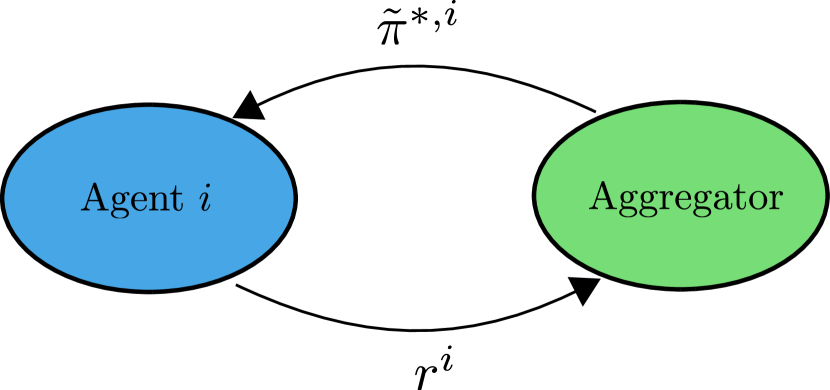
(b) Output Perturbation

Figure 1: The flow of information for (a) input perturbation and (b) output perturbation. In input perturbation, agent $i$ sends the aggregator its privatized reward function $\tilde{r}^{i}$, while in output perturbation, agent $i$ sends the sensitive (non-privatized) reward function $r^{i}$. By privatizing their reward before sending it, agents using input perturbation have greater control of the strength of privacy used to protect their rewards, and the variance of the noise needed to provide privacy is less than that of output perturbation.

Remark 4.

For input perturbation, adjacency in the sense of Definition 3 implies that every agent’s reward may differ in up to one entry by an amount up to $b$, and these are the differences that must be masked by privacy.

We next state a theorem proving that input perturbation, i.e., Algorithm 1, is $(\epsilon,\delta)$-differentially private.

Theorem 1 (Solution to Problem 1).

Given privacy parameters $\epsilon>0$, $\delta\in[0,0.5)$, and adjacency parameter $b>0$, the mapping from $\{r^{i}\}_{i\in[N]}$ to $\{\pi^{*,i}\}_{i\in[N]}$ defined by Algorithm 1 keeps each $r^{i}$ $(\epsilon,\delta)$-differentially private with respect to the adjacency relation in Definition 3.

Proof.

Setting $\sigma=\frac{b}{2\epsilon}\kappa(\epsilon,\delta)$, the result immediately follows from Lemma 1 and Lemma 2 because the computation of $\{\tilde{\pi}^{*,i}\}_{i\in[N]}$ is simply post-processing of differentially private data. ∎

Using Algorithm 1, each agent enforces the privacy of its own reward function before sending it to the aggregator. Performing input perturbation this way enforces differential privacy on a per-agent basis, which is referred to as “local differential privacy” [32]. The main advantage of input perturbation is that the aggregator does not need to be trusted since it is only sent privatized information. The flow of information for input and output perturbation is seen in Figure 1. Another advantage is that agents may select differing levels of privacy. However, to provide a fair comparison with output perturbation, the preceding implementation considers each agent using the same $\epsilon$ and $\delta$.

III-C Output Perturbation

In output perturbation, for all $i\in[N]$ agent $i$ sends its sensitive (non-private) vector rewards, $R^{i}$, to the aggregator. Then the aggregator uses these rewards to form the joint reward $R$. For privacy, noise is added to the joint reward vector, namely $\tilde{R}=R+w$, where $w\sim\mathcal{N}(0,\sigma^{2}I)$. Similar to the input perturbation setup, computing the joint policy using the privatized $\tilde{R}$ is differentially private because computation of the policy is post-processing of private data; this $\tilde{R}$ can be related to a function $\tilde{r}$ in the obvious way. Algorithm 2 presents this method of computing policies when reward functions are privatized using output perturbation.

Inputs: $\{r^{i}\}_{i\in[N]}$, $\mathcal{S}$, $\mathcal{A}$, $\gamma$, $\mathcal{T}$, $\epsilon$, $\delta$, $b$, $N$;

Outputs: Privacy-preserving policies $\{\tilde{\pi}^{*,i}\}_{i\in[N]}$;

for all $i\in[N]$ in parallel do

      Agent $i$ sends reward $r^{i}$ to the aggregator

end

Aggregator generates joint reward function: $r(s_{j},a_{k})=J(\{r^{i}(s_{j},a^{i}_{I_{k}(i)}\}_{i\in[N]})$ for all $j\in[n]$ and $k\in[m]$;

Aggregator sets $\sigma=\frac{b}{2\epsilon N}\kappa(\epsilon,\delta)\mu$;

Aggregator generates private reward function with the Gaussian mechanism, $\tilde{R}=R+w$;

Aggregator generates optimal joint policy, $\tilde{\pi}^{*}=\operatorname*{arg\,max}_{\pi}E\left[\sum_{t=0}^{\infty}\gamma^{t}\tilde{r}(s_{t},\pi(s_{t}))\right]$;

Aggregator sends $\tilde{\pi}^{*,i}$ to agent $i$ for all $i\in[N]$

Algorithm 2 Private Policy Synthesis via Output Perturbation

Remark 5.

For output perturbation, adjacency in the sense of Definition 3 implies only a single agent’s reward may change. If we regard the collection of vectorized rewards sent to the aggregator as a single vector, then adjacency in Definition 3 says that only a single entry in this vector can change. Thus, adjacency in the setting of output perturbation allows only a single agent’s reward to change, and it can change by an amount of up to $b$. However, given the mapping $J$ in (1) between all agents’ rewards and the joint reward, this difference will affect the joint reward in several places. We account for this fact next in calibrating the noise required for privacy.

We now state a theorem showing that output perturbation, i.e., Algorithm 2, is $(\epsilon,\delta)$-differentially private.

Theorem 2 (Alternative Solution to Problem 1).

Fix privacy parameters $\epsilon>0$, $\delta\in[0,0.5)$, and adjacency parameter $b>0$. Set $\mu=\max_{j\in[n]}\prod_{\begin{subarray}{c}\ell=1\\ \ell\neq j\end{subarray}}^{N}m_{\ell}$. The mapping from $\{r^{i}\}_{i\in[N]}$ to $\{\pi^{*,i}\}_{i\in[N]}$ defined by Algorithm 2 keeps each $r^{i}$ $(\epsilon,\delta)$-differentially private with respect to the adjacency relation in Definition 3.

Proof.

From Lemma 1, Algorithm 2 is differentially private if $\sigma$ is chosen according to

$$\sigma\geq\frac{\Delta_{2}J}{2\epsilon}\kappa(\epsilon,\delta).$$ (7)

We now compute $\Delta_{2}J$ and substitute into (7), which will complete the proof, since the computation of $\tilde{\pi}^{*,i}$ is differentially private in accordance with Lemma 2 by virtue of being post-processing of differentially private data.

For each $i\in[N]$, let $r^{i}$ and $\hat{r}^{i}$ denote two adjacent reward functions and let $R^{i}$ and $\hat{R}^{i}$ denote their vectorized forms as defined in (6). Then

$$R=\frac{1}{N}\Big{[}\sum_{i\in[N]}r^{i}\left(s_{1},a^{i}_{I_{1}(i)}\right),\sum_{i\in[N]}r^{i}\left(s_{1},a^{i}_{I_{2}(i)}\right),\cdots\\ \sum_{i\in[N]}r^{i}\left(s_{1},a^{i}_{I_{m}(i)}\right),\sum_{i\in[N]}r^{i}\left(s_{2},a^{i}_{I_{1}(i)}\right),\cdots\\ \sum_{i\in[N]}r^{i}\left(s_{n},a^{i}_{I_{m}(i)}\right)\Big{]}^{T}\in\mathbb{R}^{nm},$$ (8)

with $\hat{R}$ defined analogously. As noted in Remark 5, $R$ and $\hat{R}$ can differ for only one agent. Suppose the index of that agent is $j$. We then determine the sensitivity from Definition 5 of $J$ as follows:

$$\Delta_{2}J=\max_{\begin{subarray}{c}\operatorname{Adj}_{b}(R^{j},\hat{R}^{j})=1\\ R^{i}=\hat{R}^{i}\end{subarray}}\left\lVert R-\hat{R}\right\rVert_{2}.$$ (9)

Since $R^{j}$ and $\hat{R}^{j}$ are $b$-adjacent, there exists some indices $k\in[n]$ and $\ell\in[m_{i}]$ such that $r^{j}(s_{k},a^{j}_{\ell})\neq\hat{r}^{j}(s_{k},a^{j}_{\ell})$ and $r^{j}(s_{c},a^{j}_{d})=\hat{r}^{j}(s_{c},a^{j}_{d})$ for all $c\in[n]\backslash\{k\}$ and $d\in[m_{i}]\backslash\{\ell\}$. Using the fact that $R^{j}$ and $\hat{R}^{j}$ are $b$-adjacent, we obtain

$$\Delta_{2}J=\max_{\begin{subarray}{c}\operatorname{Adj}_{b}(R^{j},\hat{R}^{j})=1\\ R^{i}=\hat{R}^{i}\end{subarray}}\frac{1}{N}\Big{\lVert}\Big{[}0,\cdots,r^{j}(s_{k},a^{j}_{\ell})-\hat{r}^{j}(s_{k},a^{j}_{\ell}),\\ \cdots,r^{j}(s_{k},a^{j}_{\ell})-\hat{r}^{j}(s_{k},a^{j}_{\ell}),\cdots,0,\cdots,0\Big{]}^{T}\Big{\rVert}_{2},$$ (10)

where $r^{j}(s_{k},a^{j}_{\ell})-\hat{r}^{j}(s_{k},a^{j}_{\ell})$ appears $\prod_{\begin{subarray}{c}\ell=1\\ \ell\neq j\end{subarray}}^{N}m_{\ell}$ times since the local action $a^{j}_{\ell}$ appears in $\prod_{\begin{subarray}{c}\ell=1\\ \ell\neq j\end{subarray}}^{N}m_{\ell}$ joint actions. Note that the indices of entries in $R$ that contain the term $r^{j}(s_{k},a^{j}_{\ell})-\hat{r}^{j}(s_{k},a^{j}_{\ell})$ depend on how the user orders the joint actions, but any convention for doing yields the same sensitivity.

Since $\|R-\hat{R}\|_{2}\leq\|R-\hat{R}\|_{1}$, we upper bound (10) as

$$\Delta_{2}J\leq\frac{1}{N}|r^{j}(s_{k},a^{j}_{\ell})-\hat{r}^{j}(s_{k},a^{j}_{\ell})|\prod_{\begin{subarray}{c}\ell=1\\ \ell\neq j\end{subarray}}^{N}m_{\ell}.$$ (11)

Additionally, from our definition of adjacency, we have

$$|r^{j}(s_{k},a^{j}_{\ell})-\hat{r}^{j}(s_{k},a^{j}_{\ell})|\leq b.$$ (12)

We then combine (11) and (12) to find

$$\Delta_{2}J\leq\frac{b}{N}\max_{j\in[n]}\prod_{\begin{subarray}{c}\ell=1\\ \ell\neq j\end{subarray}}^{N}m_{\ell}=\frac{b}{N}\mu,$$ (13)

which we then substitute into (7) to find

$$\sigma\geq\frac{b}{2\epsilon N}\kappa(\epsilon,\delta)\mu,$$ (14)

which, combined with Lemma 2, completes the proof. ∎

Unlike input perturbation, output perturbation requires that agents trust the aggregator with their sensitive information. Additionally, all agents will have the same level of privacy.

Contrary to some other privacy literature, we expect significantly better performance using input perturbation over output perturbation for an increasing number of agents at a given $\epsilon$. For output perturbation, the standard deviation $\sigma$ used to calibrate the noise added for privacy essentially grows exponentially with the number of agents, which can be seen in the term $\mu$. This is because we consider the joint state $s$ in evaluating $r^{i}(s,a^{i})$ and each joint state-local action pair will appear many times in $\Delta_{2}J$. In the case of input perturbation, since the joint reward is computed from privatized rewards, the standard deviation of privacy noise does not depend on the number of agents. The standard deviations for varying $N$ and $\epsilon$ are shown in Table I(a) and Table I(b), respectively. Table I(a) shows that the variance of privacy noise is constant for input perturbation for all $N$, while for output perturbation it grows rapidly with $N$. Table I(b) shows that the variance of noise needed for input perturbation is less than that needed for output perturbation for the same level of privacy, quantified by $\epsilon$, when $N>1$.

$N$	Algo. 1	Algo. 2
$1$	$2.524$	$2.524$
$2$	$2.524$	$5.049$
$5$	$2.524$	$129.3$
$10$	$2.524$	$66,174$

(a)

$\epsilon$	Algo. 1	Algo. 2
$0.1$	23.48	46.95
$1$	2.524	5.049
$5$	0.6251	1.250
$10$	0.3684	0.7367

(b)

TABLE I: Standard Deviation required to provide differential privacy with (a) $\epsilon=1$ for varying $N$ and (b) $N=2$ for varying $\epsilon$. In (a), we see the standard deviation of privacy noise is constant for input perturbation for all $N$, while for output perturbation it grows rapidly with $N$. In (b), the standard deviation of noise needed for input perturbation is less than that needed for output perturbation for the same level of privacy, quantified by $\epsilon$, when $N>1$.

Remark 6.

Given the significantly lower standard deviation for input perturbation versus output perturbation at a given $\epsilon$ for $N>1$, we focus on input perturbation going forward unless stated otherwise.

The difference in performance between input and output perturbation is explored further in Example 1 in Section VI. In the next section, we analyze the accuracy of the privatized rewards and quantify privacy-accuracy trade-offs.

IV Accuracy Analysis

In this section, we solve Problem 2. Specifically, we analyze the accuracy of the reward functions that are privatized using input perturbation. To do so, we compute an upper bound on the expected maximum absolute error between the sensitive, non-private joint reward $r$ and the privatized reward $\tilde{r}$, namely $\mathbb{E}\left[\max_{k,j}\left|\tilde{r}(s_{k},a_{j})-r(s_{k},a_{j})\right|\right]$. Then we use this accuracy bound to develop guidelines for calibrating privacy, i.e., guidelines for choosing $\epsilon$ given some bound on allowable maximum error, $A$. The maximum absolute error is bounded as follows.

Theorem 3 (Solution to Problem 2).

Fix privacy parameters $\epsilon>0$, $\delta\in[0,0.5)$, adjacency parameter $b>0$, and MMDP $\mathcal{M}=(\mathcal{S},\mathcal{A},r,\gamma,\mathcal{T})$ with $N$ agents, $n$ joint states, and $m$ joint actions. Let $\tilde{r}$ be defined as in Algorithm 1. Then

$$\mathbb{E}\left[\max_{k,j}\left|\tilde{r}(s_{k},a_{j})-r(s_{k},a_{j})\right|\right]\leq\frac{Cb}{2\epsilon}\kappa(\epsilon,\delta)$$ (15)

where $C=\sqrt{\frac{2}{N\pi}}+\sqrt{\left(1-\frac{2}{\pi}\right)\frac{(nm-1)}{N}}$.

Proof.

First we analyze the vectorized rewards $R$ and $\tilde{R}$. Since $\tilde{r}^{i}$ is generated using Algorithm 1, we have $\tilde{r}^{i}(s_{k},a^{i}_{I_{j}(i)})=r^{i}(s_{k},a^{i}_{I_{j}(i)})+w^{k}_{I_{j}(i)}$, where $w^{k}_{I_{j}(i)}\sim\mathcal{N}(0,\sigma^{2})$. For any $s_{k}\in\mathcal{S}$ and $a_{j}\in\mathcal{A}$ the corresponding entry of $\tilde{R}-R$ is

$$\frac{1}{N}\sum_{i\in[N]}\tilde{r}^{i}(s_{k},a^{i}_{I_{j}(i)})-r^{i}(s_{k},a^{i}_{I_{j}(i)})=\frac{1}{N}\sum_{i\in[N]}w^{k}_{I_{j}(i)}.$$ (16)

Thus, the entirety of $\tilde{R}-R$ is

$$\tilde{R}-R=\frac{1}{N}\Big{[}\sum_{i\in[N]}w^{1}_{I_{1}(i)},\sum_{i\in[N]}w^{1}_{I_{2}(i)},\cdots,\\ \sum_{i\in[N]}w^{2}_{I_{1}(i)},\sum_{i\in[N]}w^{2}_{I_{2}(i)},\cdots,\sum_{i\in[N]}w^{n}_{I_{m}(i)}\Big{]}^{T}.$$ (17)

Let $y_{\ell}$ be the $\ell^{th}$ entry of $\tilde{R}-R$. Now the maximum absolute error over the entries is denoted

$$\mathbb{E}\left[\max_{\ell}\left|y_{\ell}\right|\right].$$ (18)

For any $\ell,$ we have $y_{\ell}\sim\mathcal{N}\left(0,\frac{\sigma^{2}}{N}\right),$ and that $\left|y_{\ell}\right|$ has a folded-normal distribution [33] because it is equal to the absolute value of a normal random variable. As a result, $\mathbb{E}\left[\left|y_{\ell}\right|\right]=\sigma\sqrt{\frac{2}{N\pi}}$ and $\text{Var}\left[\left|y_{\ell}\right|\right]=\frac{\sigma^{2}}{N}\left(1-\frac{2}{\pi}\right).$

To upper bound (18) we apply Equation (4) from [34] with $k=nm$ which gives

$$\mathbb{E}\left[\max_{\ell}\left|y_{\ell}\right|\right]\leq\mathbb{E}\left[\left|y_{\ell}\right|\right]+\sqrt{\text{Var}\left[\left|y_{\ell}\right|\right](nm-1)}\\ =\sigma\sqrt{\frac{2}{N\pi}}+\sqrt{\frac{\sigma^{2}}{N}\left(1-\frac{2}{\pi}\right)(nm-1)}\\ =\left(\sqrt{\frac{2}{N\pi}}+\sqrt{\left(1-\frac{2}{\pi}\right)\frac{(nm-1)}{N}}\right)\sigma.$$ (19)

Substituting $\sigma=\frac{b}{2\epsilon}\kappa(\epsilon,\delta)$ gives the expression of interest. ∎

Corollary 1.

Fix $\delta\in[0,0.5)$ and let the conditions from Theorem 3 hold. A sufficient condition to achieve $\mathbb{E}\left[\max_{k,j}|\tilde{r}(s_{k},a_{j})-r(s_{k},a_{j})|\right]\leq A$ is given by

$$\epsilon\geq\frac{2C^{2}b^{2}}{4A^{2}}+\frac{Cb\mathcal{Q}^{-1}(\delta)}{A},$$ (20)

where $C=\sqrt{\frac{2}{N\pi}}+\sqrt{\left(1-\frac{2}{\pi}\right)\frac{(nm-1)}{N}}.$

Proof.

Ensuring that the upper bound from Theorem 3 is less than or equal to $A$ provides a sufficient condition for $\mathbb{E}\left[\max_{k,j}|\tilde{r}(s_{k},a_{j})-r(s_{k},a_{j})|\right]\leq A.$ We solve for a condition on $\epsilon$ as follows,

$$\frac{Cb}{2\epsilon}\left(\mathcal{Q}^{-1}(\delta)+\sqrt{\mathcal{Q}^{-1}(\delta)^{2}+2\epsilon}\right)\leq A\\ \sqrt{\mathcal{Q}^{-1}(\delta)^{2}+2\epsilon}\leq\frac{2A\epsilon}{Cb}-\mathcal{Q}^{-1}(\delta)\\ {\mathcal{Q}^{-1}(\delta)^{2}+2\epsilon}\leq\left(\frac{2A\epsilon}{Cb}-\mathcal{Q}^{-1}(\delta)\right)^{2}=\\ \frac{4A^{2}}{C^{2}b^{2}}\epsilon^{2}-\frac{4A\mathcal{Q}^{-1}(\delta)}{Cb}\epsilon+\mathcal{Q}^{-1}(\delta)^{2}.$$ (21)

Rearranging (21) gives

$$0\leq\frac{4A^{2}}{C^{2}b^{2}}\epsilon^{2}-\left(\frac{4A\mathcal{Q}^{-1}(\delta)}{Cb}+2\right)\epsilon=\\ \epsilon\left(\frac{4A^{2}}{C^{2}b^{2}}\epsilon-\frac{4A\mathcal{Q}^{-1}(\delta)}{Cb}-2\right).$$ (22)

Since $\epsilon>0$, (22) holds as long as

$$\frac{4A^{2}}{C^{2}b^{2}}\epsilon-\frac{4A\mathcal{Q}^{-1}(\delta)}{Cb}-2\geq 0.$$ (23)

Rearranging (23) we find

$$\epsilon\geq\frac{C^{2}b^{2}}{4A^{2}}\left(2+\frac{4A\mathcal{Q}^{-1}(\delta)}{Cb}\right)=\frac{2C^{2}b^{2}}{4A^{2}}+\frac{Cb\mathcal{Q}^{-1}(\delta)}{A},$$ (24)

which completes the proof. ∎

Theorem 3 shows that the accuracy of the privatized rewards depends on the size of the MMDP $nm$, the number of agents $N$, and the privacy parameters $\epsilon$, $\delta$, and $b$, and is shown in Figure 2(a). Corollary 1 provides a trade-off between privacy and accuracy that allows users to design the strength of privacy $\epsilon$ according to some expected maximum absolute error, $A$. Figure 2(b) shows this bound for an example MMDP with $\delta=0.01$, $nm=8$, and $b=1$. In the next section we discuss an algorithm for computing the long term performance loss due to privacy in terms of the value function.

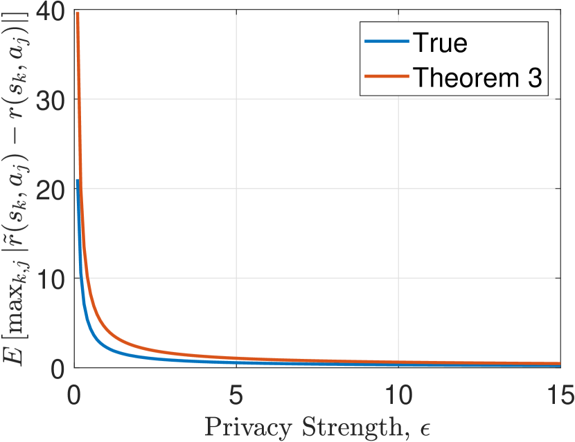
(a)

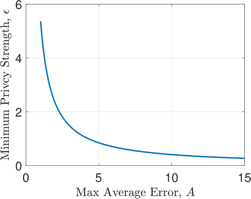
(b)

Figure 2: Simulation of (a) Theorem 3 and (b) Corollary 1 with $\delta=0.01$, $nm=8$, and $b=1$. In (a), we see that Theorem 3 captures the qualitative behavior of the empirically computed expected maximal error, while also providing accurate numerical estimates of the true maximal error. In (b), increasing privacy strength (decreasing $\epsilon$) from $\epsilon=3$ to $\epsilon=2$ leads to negligible increases in maximum average error. Furthermore, the change in maximum average error is small until $\epsilon\leq 2,$ indicating marginal performance losses until privacy is strong.

V Cost of Privacy

In this section, we solve Problem 3. To do so, we compare (i) an optimal policy generated on the original, non-private reward functions, denoted $\pi^{*}$, and (ii) an optimal policy generated on the privatized reward functions, denoted $\tilde{\pi}^{*}$. Beginning at some state $s_{0}\in\mathcal{S}$, the function $V_{\pi^{*}}(s_{0})$ encodes the performance of the MMDP given the optimal policy and $V_{\tilde{\pi}^{*}}(s_{0})$ encodes the performance of the MMDP given the policy generated on private rewards. We analyze the loss in performance due to privacy, and we refer to the “cost of privacy” metric introduced in [20], namely $|V_{\tilde{\pi}^{*}}(s_{0})-V_{\pi^{*}}(s_{0})|$, for quantifying this performance loss. Thus, we must compute $V_{\pi^{*}}(s_{0})$ and $V_{\tilde{\pi}^{*}}(s_{0})$ to quantify the cost of privacy. Note that there is not a closed form for computing a value function $V_{\pi}$ in general. Proposition 1 provides a method for empirically evaluating the value function for a policy on a given MMDP. We can then compute the cost of privacy numerically for any problem using an off-the-shelf policy-evaluation algorithm, and we compute the computational complexity of doing so. Next, we state a theorem on the number of operations required to compute the cost of privacy:

Theorem 4 (Solution to Problem 3).

Fix privacy parameters $\epsilon>0$, $\delta\in[0,1/2)$. Let $\tilde{r}$ be the output of Algorithm 1. Given an MMDP $\mathcal{M}=(\mathcal{S},\mathcal{A},r,\gamma,\mathcal{T})$, the number of computations required to compute the cost of privacy $|V_{\tilde{\pi}^{*}}(s_{0})-V_{\pi^{*}}(s_{0})|$ to within $\eta$ of the exact value is

$$nm\left(\left\lceil\frac{\log\left[\frac{4R_{\text{max}}}{\eta(1-\gamma)^{2}}\right]}{\log\left(\frac{1}{\gamma}\right)}\right\rceil+\left\lceil\frac{\log\left[\frac{4\tilde{R}_{\text{max}}}{\eta(1-\gamma)^{2}}\right]}{\log\left(\frac{1}{\gamma}\right)}\right\rceil\right),$$ (25)

where $R_{\text{max}}=\max_{s,a}|r(s,a)|$ and $\tilde{R}_{\text{max}}=\max_{s,a}|\tilde{r}(s,a)|$.

Proof.

First, given the cost of privacy,

$$|V_{\tilde{\pi}^{*}}(s_{0})-V_{\pi^{*}}(s_{0})|$$ (26)

let $V^{k}_{\tilde{\pi}}(s_{0})$ be the estimated value of $V_{\tilde{\pi}^{*}}(s_{0})$ at iteration $k$. Additionally, let $V^{k}_{\pi}(s_{0})$ be the estimated value of $V_{\pi^{*}}(s_{0})$ at iteration $k$. Then we have

$$|V^{k}_{\tilde{\pi}}(s_{0})+V^{k}_{\pi}(s_{0})-V_{\tilde{\pi}^{*}}(s_{0})-V_{\pi^{*}}(s_{0})|\\ \leq|V^{k}_{\tilde{\pi}}(s_{0})-V_{\tilde{\pi}^{*}}(s_{0})|+|V^{k}_{\pi}(s_{0})-V_{\pi^{*}}(s_{0})|$$ (27)

Accordingly, $|V^{k}_{\tilde{\pi}}(s_{0})-V_{\tilde{\pi}^{*}}(s_{0})|$ and $|V^{k}_{\pi}(s_{0})-V_{\pi^{*}}(s_{0})|$ must be approximated to $\frac{\eta}{2}$ for the cost of privacy to be within $\eta$ of its exact value. Next, we define $R_{\text{max}}=\max_{(s,a)\in\mathcal{S}\times\mathcal{A}}|r(s,a)|$ and $\tilde{R}_{\text{max}}=\max_{(s,a)\in\mathcal{S}\times\mathcal{A}}|\tilde{r}(s,a)|$. This then admits some non-private and private maximum value functions, denoted $v_{\text{max}}$ and $\tilde{v}_{\text{max}}$, respectively, since $v_{\text{max}}\leq\frac{R_{\text{max}}}{1-\gamma}$ and $\tilde{v}_{\text{max}}\leq\frac{\tilde{R}_{\text{max}}}{1-\gamma}$. From Proposition 1, we know that, given the value function at convergence, namely $v_{\infty}$, and the value function at iteration $k+1$, namely $v_{k+1}$, we have

$$\left\lVert v_{k+1}-v_{\infty}\right\rVert_{\infty}=\left\lVert\mathcal{L}v_{k}-\mathcal{L}v_{\infty}\right\rVert\leq\gamma\left\lVert v_{k}-v_{\infty}\right\rVert_{\infty},$$ (28)

which implies

$$\left\lVert v_{k+1}-v_{\infty}\right\rVert_{\infty}\leq\frac{\gamma^{k}}{1-\gamma}\left\lVert v_{1}-v_{0}\right\rVert_{\infty}\leq\frac{2\gamma^{k}v_{\text{max}}}{1-\gamma},$$ (29)

where $v_{0}$ is the initial guess of the value function and $v_{1}$ is the value function after $1$ iteration of policy evaluation. However, $v_{\text{max}}$ may not be known exactly. As a result, we upper bound (29) using $v_{\text{max}}\leq\frac{R_{\text{max}}}{1-\gamma}$ to find

$$\frac{2\gamma^{k}v_{\text{max}}}{1-\gamma}\leq\frac{2\gamma^{k}R_{\text{max}}}{(1-\gamma)^{2}}.$$ (30)

To compute the non-private value function $V_{\pi^{*}}$ within $\eta$ of the limiting value, we wish to find the number of iterations of policy evaluation such that

$$\frac{2\gamma^{k}R_{\text{max}}}{(1-\gamma)^{2}}\leq\frac{\eta}{2}.$$ (31)

We then rearrange (31) to find

$$K_{1}=\left\lceil\frac{\log\left[\frac{4R_{\text{max}}}{\eta(1-\gamma)^{2}}\right]}{\log\left(\frac{1}{\gamma}\right)}\right\rceil.$$ (32)

Following an identical construction, for computing the private value function $V_{\tilde{\pi}^{*}}$ to within $\eta$ of its exact value we have that

$$K_{2}=\left\lceil\frac{\log\left[\frac{4\tilde{R}_{\text{max}}}{\eta(1-\gamma)^{2}}\right]}{\log\left(\frac{1}{\gamma}\right)}\right\rceil$$ (33)

iterations of policy evaluation are required. Therefore, the total number of iterations of policy evaluation required to determine the cost of privacy is

$$K=K_{1}+K_{2}=\left\lceil\frac{\log\left[\frac{4R_{\text{max}}}{\eta(1-\gamma)^{2}}\right]}{\log\left(\frac{1}{\gamma}\right)}\right\rceil+\left\lceil\frac{\log\left[\frac{4\tilde{R}_{\text{max}}}{\eta(1-\gamma)^{2}}\right]}{\log\left(\frac{1}{\gamma}\right)}\right\rceil.$$ (34)

Additionally, each iteration of policy evaluation requires looping through all $nm$ values of the reward function. As a result, the total number of computations required to compute the cost of privacy within $\eta$ of its exact value is

$$nm\left(\left\lceil\frac{\log\left[\frac{4R_{\text{max}}}{\eta(1-\gamma)^{2}}\right]}{\log\left(\frac{1}{\gamma}\right)}\right\rceil+\left\lceil\frac{\log\left[\frac{4\tilde{R}_{\text{max}}}{\eta(1-\gamma)^{2}}\right]}{\log\left(\frac{1}{\gamma}\right)}\right\rceil\right).$$

∎

In words, $nm$ is the number of computations required within each iteration of policy evaluation, while the term in the parentheses is the number of iterations of policy evaluation required. If $\pi^{*}$ is generated using value iteration, the user already has access to $V_{\pi^{*}}$ and thus does not need to compute it again for the cost of privacy. In this case, only $V_{\tilde{\pi}^{*}}$ needs to be computed. However, we state the total number of computations required assuming the user only has access to $\pi^{*}$ and $\tilde{\pi}^{*}$.

VI Numerical Simulations

In this section, we consider two MDPs to numerically simulate the results discussed in this work. First, we consider a small $2\times 2$ gridworld example to discuss the cost of privacy with multiple agents, and then we consider a larger MDP with a single agent to assess how differential privacy changes a state trajectory over time. To compare the change in value between input perturbation and output perturbation, consider the following example comparing their costs of privacy.

Example 1 (Gridworld).

Consider the $2\times 2$ gridworld environment from Figure 3(a) with $N=2$ agents whose goal is for both agents to occupy state $0$. The set of local agent actions is $\mathcal{A}^{i}=\{\texttt{left},\texttt{right},\texttt{up},\texttt{down},\texttt{stay}\}$ with $r^{i}(s,a^{i})=-1$ for all $s\in\mathcal{S}$ and $a^{i}\in\mathcal{A}^{i}\setminus\{\texttt{stay}\}$ and $r^{i}((0,0),\texttt{stay})=1$. For any action $a^{i}\in\mathcal{A}^{i}$, the probability of agent $i$ slipping into a state not commanded by the action is $p=0.1$. We consider the adjacency parameter $b=3$ and privacy parameters $\epsilon\in[0.1,15]$ and $\delta=0.01$. Figure 3(b) shows a sample environment with $\epsilon=1$. Simulating this environment with $N=2$ agents, Figure 4 shows the change in utility with decreasing strength of privacy (quantified by growing $\epsilon$).

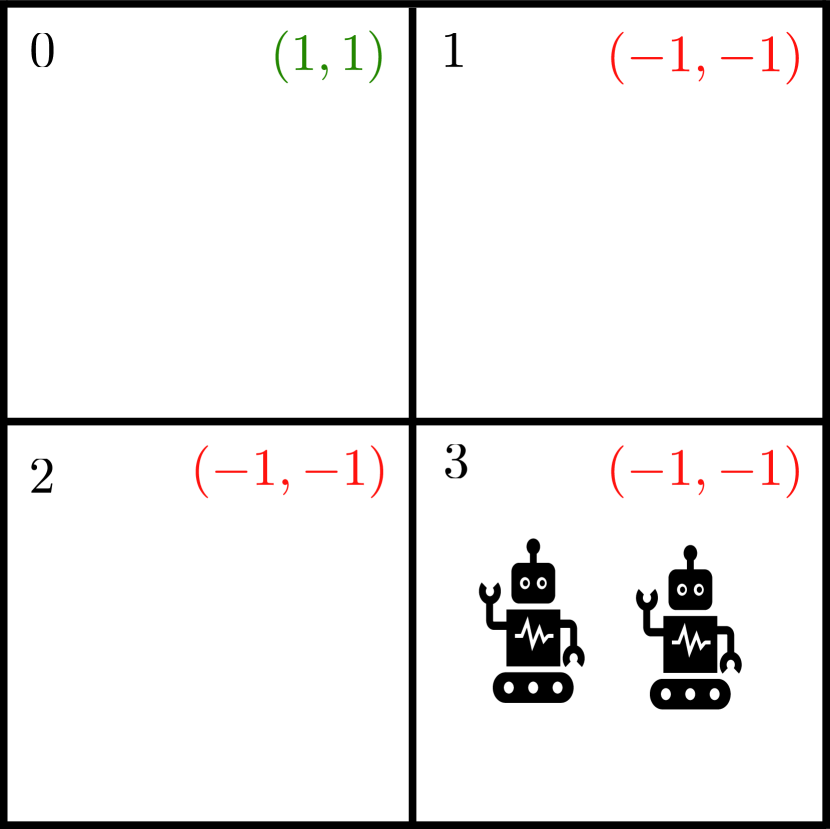
(a) Non-private rewards

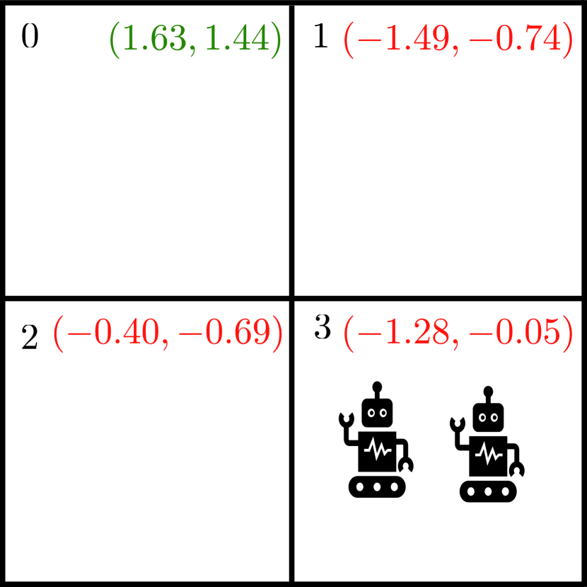
(b) Privatized rewards

Figure 3: Multi-agent Gridworld from Example 1 with (a) non-private rewards and (b) privatized rewards. The local state number is in black, and each agent’s reward for both agents taking the action $a^{i}=\texttt{stay}$ at a given local state is colored green for the state with the max reward and red for all others. Even under privacy, the goal state-action pair remains unchanged in this example.

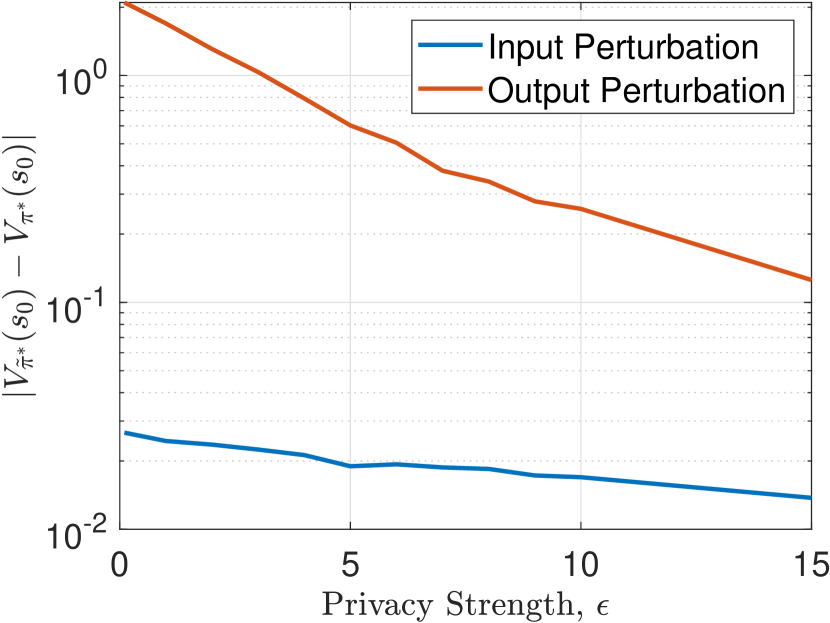
Figure 4: The values of $|V_{\tilde{\pi}^{*}}(s_{0})-V_{\pi^{*}}(s_{0})|$ for the $2\times 2$ gridworld in Example 1, averaged over $5,000$ samples at each $\epsilon$ with $\epsilon\in[0.1,15]$. We see input perturbation with a lower cost of privacy for all values of $\epsilon$, with output perturbation being outperformed by input perturbation even with input perturbation being strongly private and output perturbation having only weak privacy.

Output perturbation has a greater cost of privacy because the variance of privacy noise has essentially exponential dependence upon the number of agents. The cost of privacy decreases with $\epsilon$ in both input and output perturbation, which agrees with how privacy should intuitively affect the performance of the MMDP. Output perturbation has a higher cost of privacy with $\epsilon=15$ than input perturbation does with $\epsilon=0.1$, indicating that even when relaxing the strength of privacy for output perturbation, input perturbation has better performance.

Example 2 (Waypoint Guidance).

To highlight the applicability to a single agent, consider a high-speed vehicle using waypoints to navigate towards a target. We consider an MDP with a $20\times 20$ set of waypoints as the states, as seen in Figure 5, with the actions $\mathcal{A}=\{\texttt{north},\texttt{south},\texttt{east},\texttt{west},\texttt{to target}\}$.

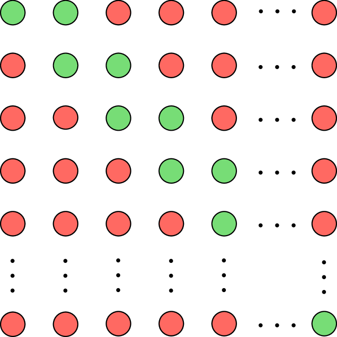
(a) Non-private rewards

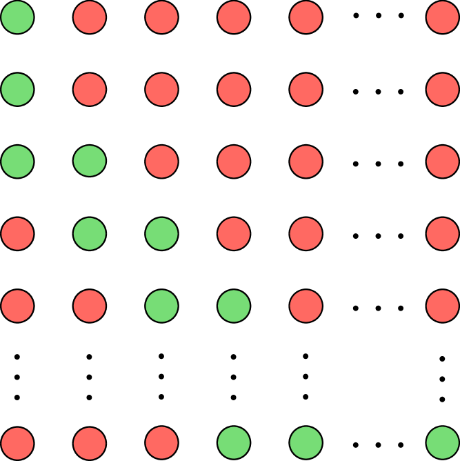
(b) Privatized rewards

Figure 5: Waypoints selected (green) by policy generated using the (a) non-private rewards and (b) private rewards. Here, the goal state remains unchanged by privacy, but the privately generated waypoints differ from the nominal waypoints and more waypoints are needed to reach the goal state.

We consider a 3 degree-of-freedom vehicle model, with waypoints that exist in the plane of the initial condition. The initial position of the vehicle is the first waypoint and the initial state of the MDP. The action for that state yields a new waypoint for the vehicle to navigate towards. Once the vehicle is closer to the new waypoint than the original, we say the new waypoint is now the current state of the vehicle, and the policy again commands the vehicle to navigate to a new waypoint. This continues until the vehicle is less than $80~{}\text{km}$ from the target, at which point the vehicle is considered to have “arrived” at its target. As a result, within $80~{}\text{km}$ it is commanded to navigate directly to the target (as opposed to another waypoint) without privacy enforced.

The optimal policy gives the optimal set of waypoints given an initial starting state. We implemented differential privacy for the reward function of this MDP using Algorithm 1. Note that since there is only one agent, the outputs of Algorithm 1 and Algorithm 2 are identical.

Trajectories generated using various $\epsilon$ values are presented in the crossrange-downrange plane in Figure 6.

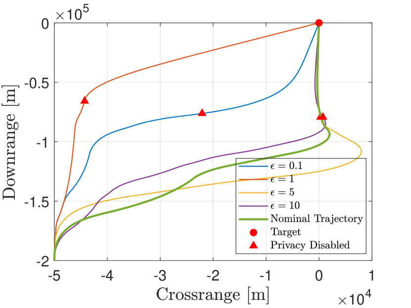
Figure 6: High-speed vehicle trajectories given varying privacy levels from Example 2. When privacy is weaker, such as at $\epsilon=10$, the trajectory of the vehicle is a close match to the nominal trajectory, while when privacy is stronger, there are more pronounced deviations from the nominal trajectory. This matches the intuition that as privacy is weakened, we should recover the nominal trajectory.

We simulated $600$ privatized policies for each $\epsilon\in[0.1,10]$. While on average we recover the nominal trajectory as epsilon grows, note that individual trajectories are random draws, and here the reward privatized with $\epsilon=1$ yielded a more off-nominal trajectory than the one privatized with $\epsilon=0.1$.

Treating the trajectory generated from the sensitive policy as the nominal trajectory, we assess the performance of the trajectories using the change in the cumulative acceleration commands, which we refer to as “control effort” and denote by $\Delta c$, between the trajectories generated using the sensitive, non-private policy and the privatized policy. That is,

$$\Delta c=\int_{0}^{t_{f}}\|u\|_{2}^{2}dt-\int_{0}^{\tilde{t}_{f}}\|\tilde{u}\|^{2}_{2}dt,$$ (35)

where $u$ is the commanded acceleration of the vehicle operating with a policy developed on the non-private rewards, and $\tilde{u}$ is defined analogously for the vehicle operating with a policy developed on the private rewards. Here $t_{f}$ is the flight duration of the vehicle when using a policy generated on sensitive, non-private reward $r$ and $\tilde{t}_{f}$ is the flight duration of the vehicle when using a policy generated on privatized rewards $\tilde{r}$. Note that under privacy, trajectories may differ in length, which means that comparing the accelerations at each time step may not yield a meaningful comparison. As a result, we compare the total commanded accelerations over the entire trajectory, shown in Figure 7. On average, with stronger privacy (i.e., smaller $\epsilon$), the policy commands the vehicle to off-nominal trajectory waypoints requiring larger overall control efforts. We see $\Delta c$ steadily declines up to $\epsilon=2$, indicating that there is minimal performance gain by decreasing the strength of privacy any further, which implies that $\epsilon=2$ effectively trades of privacy and performance in this case.

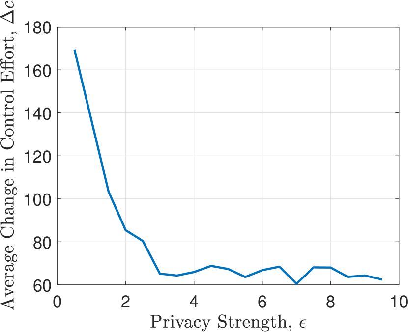
Figure 7: Average control effort for $600$ private policies generated with $\epsilon\in[0.1,10]$. As the strength of privacy decreases (and $\epsilon$ increases), the change in control effort decreases. The optimal policy induces the least amount of turning in the vehicle, which requires less control effort, but private policies may require sharp turns to force the vehicle to reach the target, inducing more control effort as a result.

VII Conclusion

We have developed two methods for protecting reward functions in MMDPs from observers by using differential privacy, and we identified input perturbation as the more tractable method. We also examined the accuracy versus privacy trade-off and the computational complexity of computing the performance loss due to privacy, and showed the success of these methods in simulation. Future work will be focused on developing guidelines for designing reward functions that are amenable to privacy.

References

- [1] D. J. Glancy, “Privacy in autonomous vehicles,” Santa Clara L. Rev., vol. 52, p. 1171, 2012.
- [2] Z. Guan, G. Si, X. Zhang, L. Wu, N. Guizani, X. Du, and Y. Ma, “Privacy-preserving and efficient aggregation based on blockchain for power grid communications in smart communities,” IEEE Communications Magazine, vol. 56, no. 7, pp. 82–88, 2018.
- [3] A. Y. Ng, S. Russell et al., “Algorithms for inverse reinforcement learning.” in Icml, vol. 1, 2000, p. 2.
- [4] B. D. Ziebart, A. L. Maas, J. A. Bagnell, A. K. Dey et al., “Maximum entropy inverse reinforcement learning.” in Aaai, vol. 8. Chicago, IL, USA, 2008, pp. 1433–1438.
- [5] T. Zhi-Xuan, J. Mann, T. Silver, J. Tenenbaum, and V. Mansinghka, “Online bayesian goal inference for boundedly rational planning agents,” Advances in neural information processing systems, vol. 33, pp. 19 238–19 250, 2020.
- [6] M. Ramırez and H. Geffner, “Goal recognition over pomdps: Inferring the intention of a pomdp agent,” in IJCAI. IJCAI/AAAI, 2011, pp. 2009–2014.
- [7] C. Dwork, “Differential privacy,” Automata, languages and programming, pp. 1–12, 2006.
- [8] J. Le Ny and G. J. Pappas, “Differentially private filtering,” IEEE Transactions on Automatic Control, vol. 59, no. 2, pp. 341–354, 2013.
- [9] J. Cortés, G. E. Dullerud, S. Han, J. Le Ny, S. Mitra, and G. J. Pappas, “Differential privacy in control and network systems,” in 55th IEEE Conference on Decision and Control (CDC), 2016, pp. 4252–4272.
- [10] S. Han and G. J. Pappas, “Privacy in control and dynamical systems,” Annual Review of Control, Robotics, and Autonomous Systems, vol. 1, pp. 309–332, 2018.
- [11] K. Yazdani, A. Jones, K. Leahy, and M. Hale, “Differentially private lq control,” IEEE Transactions on Automatic Control, 2022.
- [12] C. Hawkins and M. Hale, “Differentially private formation control,” in 2020 59th IEEE Conference on Decision and Control (CDC). IEEE, 2020, pp. 6260–6265.
- [13] Y. Wang, M. Hale, M. Egerstedt, and G. E. Dullerud, “Differentially private objective functions in distributed cloud-based optimization,” in 2016 IEEE 55th Conference on Decision and Control (CDC). IEEE, 2016, pp. 3688–3694.
- [14] Z. Huang, S. Mitra, and N. Vaidya, “Differentially private distributed optimization,” in Proceedings of the 16th International Conference on Distributed Computing and Networking, 2015, pp. 1–10.
- [15] S. Han, U. Topcu, and G. J. Pappas, “Differentially private distributed constrained optimization,” IEEE Transactions on Automatic Control, vol. 62, no. 1, pp. 50–64, 2016.
- [16] E. Nozari, P. Tallapragada, and J. Cortés, “Differentially private distributed convex optimization via objective perturbation,” in 2016 American control conference (ACC). IEEE, 2016, pp. 2061–2066.
- [17] R. Dobbe, Y. Pu, J. Zhu, K. Ramchandran, and C. Tomlin, “Customized local differential privacy for multi-agent distributed optimization,” arXiv preprint arXiv:1806.06035, 2018.
- [18] Y.-W. Lv, G.-H. Yang, and C.-X. Shi, “Differentially private distributed optimization for multi-agent systems via the augmented lagrangian algorithm,” Information Sciences, vol. 538, pp. 39–53, 2020.
- [19] C. Dwork, A. Roth et al., “The algorithmic foundations of differential privacy,” Foundations and Trends in Theoretical Computer Science, vol. 9, no. 3–4, pp. 211–407, 2014.
- [20] P. Gohari, M. Hale, and U. Topcu, “Privacy-preserving policy synthesis in markov decision processes,” in 2020 59th IEEE Conference on Decision and Control (CDC). IEEE, 2020, pp. 6266–6271.
- [21] B. Chen, C. Hawkins, M. O. Karabag, C. Neary, M. Hale, and U. Topcu, “Differential privacy in cooperative multiagent planning,” arXiv preprint arXiv:2301.08811, 2023.
- [22] P. Venkitasubramaniam, “Privacy in stochastic control: A markov decision process perspective,” in 51st Annual Allerton Conference on Communication, Control, and Computing, 2013, pp. 381–388.
- [23] X. Zhou, “Differentially private reinforcement learning with linear function approximation,” Proceedings of the ACM on Measurement and Analysis of Computing Systems, vol. 6, no. 1, pp. 1–27, 2022.
- [24] P. Ma, Z. Wang, L. Zhang, R. Wang, X. Zou, and T. Yang, “Differentially private reinforcement learning,” in International Conference on Information and Communications Security. Springer, 2019, pp. 668–683.
- [25] B. Fallin, C. Hawkins, B. Chen, P. Gohari, A. Benvenuti, U. Topcu, and M. Hale, “Differential privacy for stochastic matrices using the matrix dirichlet mechanism,” in 2023 62nd IEEE Conference on Decision and Control (CDC). IEEE, 2023, pp. 5067–5072.
- [26] B. Chen, K. Leahy, A. Jones, and M. Hale, “Differential privacy for symbolic systems with application to markov chains,” Automatica, vol. 152, p. 110908, 2023.
- [27] D. Ye, T. Zhu, W. Zhou, and S. Y. Philip, “Differentially private malicious agent avoidance in multiagent advising learning,” IEEE transactions on cybernetics, vol. 50, no. 10, pp. 4214–4227, 2019.
- [28] C. Boutilier, “Planning, learning and coordination in multiagent decision processes,” in TARK, vol. 96. Citeseer, 1996, pp. 195–210.
- [29] M. L. Puterman, Markov decision processes: discrete stochastic dynamic programming. John Wiley & Sons, 2014.
- [30] J. Hsu, M. Gaboardi, A. Haeberlen, S. Khanna, A. Narayan, B. C. Pierce, and A. Roth, “Differential privacy: An economic method for choosing epsilon,” in 2014 IEEE 27th Computer Security Foundations Symposium. IEEE, 2014, pp. 398–410.
- [31] C. Hawkins, B. Chen, K. Yazdani, and M. Hale, “Node and edge differential privacy for graph laplacian spectra: Mechanisms and scaling laws,” arXiv preprint arXiv:2211.15366, 2022.
- [32] J. C. Duchi, M. I. Jordan, and M. J. Wainwright, “Local privacy and statistical minimax rates,” in 2013 IEEE 54th Annual Symposium on Foundations of Computer Science. IEEE, 2013, pp. 429–438.
- [33] F. C. Leone, L. S. Nelson, and R. Nottingham, “The folded normal distribution,” Technometrics, vol. 3, no. 4, pp. 543–550, 1961.
- [34] B. C. Arnold and R. A. Groeneveld, “Bounds on expectations of linear systematic statistics based on dependent samples,” The Annals of Statistics, pp. 220–223, 1979.