CRIRES-POP: a library of high resolution spectra in the near-infrared. III. Line identification in the K-giant 10 Leo

Abstract

Context. High-resolution spectra in the near-infrared (NIR) are an important tool for the detailed study of stellar atmospheres. The accurate identification of elements and molecules in these spectra can be used to determine chemical abundances and physical conditions in the photosphere of the observed star. Such identifications require precise line positions and strengths of both atomic and molecular features.

Aims. This work focusses on the full identification of absorption lines in the NIR spectrum of the K-giant 10 Leo, including previously unidentified lines. The large number and complexity of the observed absorption lines require a deep search for potential spectral signatures to enable an unambiguous assignment to specific elements or molecular species. We aim to improve the published line lists of metals, some of which are determined by model calculations only, and many of which presently lack the completeness and accuracy of line parameters.

Methods. The CRIRES-POP project provided high-resolution, high signal-to-noise ratio (S/N) spectra of several bright stars in the 1 to 5 $\mu$m range. For the K-giant 10 Leo, a spectrum corrected for telluric absorption and with precise wavelength calibration is available. This has been analysed by comparison with model spectra and up-to-date line lists.

Results. We identified lines of 29 elements and eight molecular species. While the positions of many known lines could be confirmed, about 6% of all lines detected in 10 Leo could not be attributed to any known feature. For CO and its isotopologues, molecular constants could be derived and several additional lines identified. We report major inconsistencies for some prominent lines. In addition, abundances for several key elements in 10 Leo are provided.

1 Introduction

Late-type stars emit the majority of their flux in the infrared, and modern infrared detectors allow for them to be studied – within the atmospheric windows – at a high signal-to-noise ratio (S/N) and with limited telluric absorption. For cool giants, a large number of molecular lines of abundant species such as CO, OH, CN, H₂O, and SiO populate the range between 1 and 5 $\mu$m. These are of key interest as tracers of the temperature stratification of the extended atmospheres, atmospheric dynamics, nucleosynthesis, and mixing processes. In addition, the infrared harbours a wealth of atomic lines; many of them, in particular within the atmospheric windows in the YJ band, have little blending.

However, to extract this kind of information from the stellar spectra, a complete and accurate catalogue of spectral lines that appear in that wavelength range is necessary. Any analysis relying on synthetic spectra to derive stellar parameters and elemental abundances is limited by the quality of the line data and the knowledge of line blends. This is true not only for high-resolution studies, but also for work based on low- to medium-resolution spectroscopy.

High-resolution near-infrared (NIR) spectroscopy became available with the Fourier Transform Spectrometers (FTS) in the 1970s, and even more so with the recent class of NIR echelle spectrographs at 8m-class telescopes, offering access to a wide range of objects to be studied. FTS spectra led to the first high-resolution spectral atlases with the Arcturus atlas (Hinkle et al., 1995b) providing the most extensive compendium to date of line identifications of a cool star in the NIR. While the lasting importance of this compendium is indisputable, similar studies are needed for a wider range of stellar reference objects to constrain effects of temperature, surface gravity, and metallicity.

The CRIRES-POP project (Lebzelter et al., 2012) obtained an observational library of high-resolution infrared stellar spectra covering the wavelength range from 1 to 5 $\mu$m for a set of stars throughout the Hertzsprung-Russell (HR) diagram. The spectra have a typical S/N of 200 at a spectral resolution R=90 000. The first star published with a full data reduction including a careful reanalysis of the wavelength calibration and telluric correction was the K-giant 10 Leo (Nicholls et al., 2017). A summary of the stellar parameters of 10 Leo is provided in that paper.

Table 1: Properties of 10 Leonis and Arcturus

Property	10 Leo	Ref.	Arcturus	Ref.
SpT	K1 IIIVAR	1	K0 III	7
Teff	4801$\pm{89}$ K	2	4286$\pm{30}$ K	8
L	59.35 L$\odot$	2	170 $\pm{8}$ L$\odot$	9
R	14 R$\odot$	2	25.4 $\pm{0.2}$ R$\odot$	8
M	2	3	1.08 $\pm{0.06}$ M$\odot$	8
log g	2.83 $\pm{0.23}$	2	1.66 $\pm{0.05}$	8
Distance	77.3 $\pm{1.5}$ pc	4	11.26$\pm{0.07}$pc	10
Age	4.51 $\pm{1.8}$ Gyr	5	$7.1_{-1.3}^{+1.5}$ Gyr	8
$[Fe/H]$	-0.03 $\pm{0.08}$	2	-0.52$\pm{0.04}$	8
vmic	1.3 km s-1	6	1.2 $\pm{0.11}$ km s-1	11

Roman, 1952, (1); da Silva et al., 2011, (2); Mishenina et al., 2006, (3); Bailer-Jones et al., 2021, (4); Soubiran et al., 2008, (5); Tan et al., 2016, (6); Gray et al., 2003, (7); Ramírez & Allende Prieto, 2011, (8); Schröder & Cuntz, M., 2007, (9); van Leeuwen, 2007, (10); Kondo et al., 2019, (11)

We briefly summarise and provide an update on the star’s most important properties in the following (Table 1): 10 Leo is a K1 giant with an effective temperature of 4800 K (da Silva et al., 2011). It is a spectroscopic binary, but no lines from the companion have been found in the infrared spectrum. The CRIRES-POP spectrum has been corrected for the corresponding orbital motion. According to Gaia Early Data Release 3 (EDR3) data (Bailer-Jones et al., 2021), the distance of 10 Leo is 77.3$\pm$1.5 pc, which is a minor increase compared to the earlier Hipparcos distance of 75 pc used in Nicholls et al. (2017). da Silva et al. (2011) found a metallicity close to solar. However, we note that the referenced age and log g in Table 1 for 10 Leo are not consistent with the other stellar parameters, and suggest a lower radius for 10 Leo and an age around 2.5 Gy based on the mass of 2 M_⊙, the reported luminosity, distance, and T_eff.

10 Leo differs in some aspects from the K-giant Arcturus. Table 1 allows for a direct comparison of the two stars. The most significant differences for our study are likely the higher temperature and the higher metallicity of 10 Leo compared to Arcturus.

In this paper, we present a detailed exploration of the spectroscopic line content in the NIR for the K-giant 10 Leo. We present a compendium of line identifications, including a substantial number of lines not identified in the Arcturus atlas; list lines lacking identification to date; and derive parameters for the molecular bands of CO and CN between 1 and 5 $\mu$m. Furthermore, we discuss the differences between the spectra of 10 Leo and Arcturus, and derive elemental abundances in 10 Leo for a set of prominent atomic species. More extensive documentation of our data analysis is provided in Zendel (2021).

2 Spectral lines

2.1 Methods of line identification

We applied two approaches to identify the lines found in the NIR spectrum of 10 Leo. First, we used the Vienna atomic line database (VALD3) provided by Ryabchikova et al. (2015) to determine all of the lines that are known or expected in the wavelength range covered. For the molecular lines of CO, CN, and OH, tables from Goorvitch (1994), Brooke et al. (2014), and the High-resolution TRANsmission (HITRAN) database from Gordon et al. (2017) were used. To select the lines visible for the stellar parameters of 10 Leo, we used the ‘extract stellar’ option from VALD3 which returns a list of lines with various spectral parameters such as wavenumber, log gf value, and damping constants for a particular model atmosphere. The chosen model atmosphere (castelli_ap00k2_T04750G30) for 10 Leo is based on T_eff=4800 K, log g=2.83, v_mic=2 km/s, and solar abundances. The minor difference to the literature value for v_mic presented in Table 1 resulted from the availability of models.

Second, we used the Arcturus atlas by Hinkle et al. (1995b). This atlas has been serving as a benchmark spectrum for high-resolution infrared spectroscopy of cool giants for decades. It was obtained with the FTS at Kitt Peak National Observatory and has a spectral resolution around 100 000. The line list for Arcturus comprises a total of 6658 absorption lines from 22 elements or ions and seven molecular species within the 1 to 5 $\mu$m range. All line identifications in the Arcturus atlas were based on laboratory spectra only. The data files for the IR spectrum of Arcturus (Hinkle et al., 1995a) cover two observation periods in 1993 and 1994.

Most of the bad pixels in the 10 Leo spectrum had already been removed by Nicholls et al. (2017), but to make sure we avoid incorrect line detections, the selection criterion was set to a minimum of three neighbouring pixels being below the continuum. Lines in the 10 Leo spectrum were detected by an automatic search for flux values more than 0.5 % below the local pseudo-continuum level. The corresponding vacuum wavelengths of the detected minima were then cross-correlated with the line lists from Arcturus, VALD3, and HITRAN.

The CRIRES-POP 10 Leo spectrum is divided into the five sections according to the atmospheric windows. We follow this division for the presentation of findings and line lists here. The 10 Leo spectrum comes with a number of gaps in wavelength that have no flux information, for example, the YJ bandpass has 226 gaps with sizes ranging from 0.04 nm to 2.1 nm, mostly due to strong telluric features. Details are described in Nicholls et al. (2017). We emphasise that our compendium does not include information from these gaps.

2.2 Identified atomic lines

Our 10 Leo NIR spectrum features a complex mixture of lines with various line shapes, a wide range of line intensities, and some discontinuities. The removal of telluric lines with the Molecfit software (Kausch et al., 2015; Smette et al., 2015) and the applied corrections of various instrumental impacts (Nicholls et al., 2017) created some artefacts in the spectrum, mainly in the form of discontinuities of the continuum. This necessitated a visual inspection of the spectrum to properly identify the spectral lines.

Table 2 provides a summary of the number of lines identified within the 10 Leo NIR spectrum sorted by bandpass. We note that these numbers include all components provided by the above described query of the VALD3 database. A significant fraction of these lines are contributions to blends. Our approach was that whenever the spectral feature showed signs of blending, we added all lines expected within the width of the blend to our line list. As is subsequently described in more detail in Sect. 3, our line compendium takes care of this issue by adding information on the complexity of the line profile to each spectral feature.

Table 3 lists the number of atomic lines identified, sorted by element and bandpass. Equivalent widths (EWs) of the strongest and weakest unblended lines are given as well. Values in parentheses refer to blended lines and should be regarded as upper limits of detection. The observed elements are grouped into alpha process elements (C, O, N, Ne, Mg, Si, Ar, and Ca), odd-Z elements (Na, Al, P, K, and Sc), iron peak elements (Ti, V, Cr, Mn, Fe, Co, and Ni), and s-process elements (Cu, Zn, Rb, Sr, Y, Zr, Ce, and Yb). In addition, lines from H and He have been identified. This distinction is ambiguous in some cases, for example, Ti, Co, and Fe can be formed by the alpha process as well. Ca, Fe, Ti, Mg, and Y are also present in ionised form, and all others are neutral except for Sr, Ce, Dy, and Yb, which are found in ionised form only.

Table 2: Overview of observed lines

wavelength	listed lines	observed linesb
range	VALD3a	identified	unidentified
YJ	4321	3664	433
H	6586	4438	303
K	4166	3018	196
L	1900	1304	415
M	3080	2577	84
SUM:	20053	15001	1431

• ^a From VALD3 stellar extraction corrected for gaps

• ^b Includes all observed lines of the 10 Leo NIR spectrum

Table 3: 10 Leo: Identified lines per element

Element	YJ	H	K	L	M	total	strongest	EW	weakest	EW
							line [nm]	[mÅ]	line [nm]	[mÅ]
H I	3	6	1	2	1	13	1681.11	232	1556.07	(6)
He I	1	0	0	0	0	1	1083,33	70
Alpha-process
C I	40	83	19	43	0	185	1069.42	117	3777.32	2
Mg I	41	85	76	75	10	287	3677.19	271	1030.21	12
Mg II	2	0	0	0	0	2	1095.48	11	1091.84	(3)
Si I	135	126	140	132	16	549	2206.87	305	1080.01	2
S I	11	21	19	2	0	53	1046.22	58	2289.35	8
Ca I	54	33	48	21	6	162	2263.10	278	2194.87	3
Ca II	5	2	4	0	0	11	1184.22	114	985.75	7
odd-Z
Na I	21	7	17	16	3	64	2208.97	331	991.87	(3)
Al I	10	10	7	9	1	37	1312.70	479	3601.13	6
P I	8	8	0	0	0	16	1058.45	16	1068.43	6
K I	7	3	2	7	0	19	1177.61	158	2194.87	3
Sc I	0	0	9	0	0	9	2207.13	34	2173.64	2
Iron-peak
Ti I	106	74	29	9	3	221	964.09	192	998.40	2
Ti II	3	7	0	0	0	10	1587.82	68	969.39	(8)
V I	10	16	8	0	0	34	1290.47	21	1318.86	2
Cr I	51	20	10	10	2	93	1101.85	77	1295.06	4
Mn I	13	36	6	6	0	61	1332.26	322	3473.88	6
Fe I	440	1205	372	393	9	2419	1188.61	325	1217.44	2
Fe II	4	5	1	0	0	10	1086.56	13	1112.85	(3)
Co I	14	26	4	0	0	44	1676.22	82	2207.29	3
Ni I	43	93	31	41	1	209	1631.50	144	1240.51	3
s-process
Cu I	0	4	0	0	0	4	1601.00	(27)	1601.09	(4)
Zn I	3	0	0	0	0	3	1305.71	17	1105.73	(9)
Rb I	0	2	0	0	0	2	1529.37	(6)
Sr II	3	0	0	0	0	3	1033.01	232	1003.94	119
Y I	0	1	5	0	0	6	1766.80	17	2255.00	5
Y II	5	0	0	0	0	5	1024.80	11	1018.93	6
Zr I	3	0	0	0	0	3	982.53	3	1166.11	2
Ce II	36	15	3	0	0	54	1708.20	56	1258.57	5
Dy II	1	0	0	0	0	1	1052.63	7
Er II	1	0	0	0	0	1	1106.26	(11)
Yb II	0	1	0	0	0	1	1650.28	(10)

• Values in parentheses refer to blended lines and should be regarded as upper limits of detection.

2.3 Molecular lines and bandheads

Many molecular species form band structures in the infrared with distinct patterns for the line positions and strengths. While this in principle eases the identification of molecular lines, some bands are blended with others complicating the analysis. The abundant molecular lines in the 10 Leo spectrum mainly stem from CO, CN, and OH molecules. Lines from the isotopologues $\@element[13]{\mathrm{C}}$$\@element[16]{\mathrm{O}}$, ¹²C$\@element[17]{\mathrm{O}}$, and ¹²C$\@element[18]{\mathrm{O}}$ are easily detectable throughout the spectrum. However, no lines of C$\@element[15]{\mathrm{N}}$ could be detected based on a search using the catalogue of CN lines from Brooke et al. (2014). Each band was fitted with a fourth order polynomial to locate the individual transition lines and to ensure consistency in transition assignment. Fundamental bands ($\Delta\nu$=1) of CO are observed in the M band, first overtone bands ($\Delta\nu$=2) in the K band, and second overtone bands ($\Delta\nu$=3) in the H band. A total of 105 CO bands (64 in M, 23 in K, and 18 in H) were evaluated which comprises about 4500 CO lines (almost twice the number of CO lines identified in the Arcturus atlas). Table 4 summarises all fundamental bands from which lines could be identified in the 10 Leo spectrum. The wavelengths given for the R0 and P1 lines of each band were computed from the polynomials deduced for each band. Central depths (cdepth) and EWs are given for the strongest detected line in each band.

Table 4: Fundamental CO bands

	R-branch				P-branch
Band-ID	$\lambda$ (R0)a	Transitionb	(1-F)	cdepthc	$\lambda$ (P1)a	Transition b	(1-F)	cdepthc
	nm				nm
CO 1-0	4657.49d	R6	0.587	0.482	4674.15d	P11	0.517	0.487
CO 2-1	4715.72	R14	0.506	0.492	4732.65	P23	0.513	0.477
CO 3-2	4775.28	R22	0.472	0.474	4792.48	P30	0.424	0.443
CO 4-3	4836.21	R29	0.419	0.441	4853.69	P17	0.397	0.416
CO 5-4	4898.54d	R34	0.373	0.400	4916.30d	P7	0.336	0.351
CO 6-5	4962.33	R31	0.332	0.365	4980.38d	P20	0.317	0.342
CO 7-6	5027.62d	R13	0.264	0.318	5045.98	P4	0.232	0.262
CO 8-7	5094.45	R25	0.253	0.301	5113.12d	P8	0.248	0.256
CO 9-8	5162.90d	R24	0.219	0.271
CO 10-9	5232.99e	R19	0.186	0.235
CO 11-10	5304.80e	R27	0.168	0.210
CO 12-11	5378.53e	R45	0.121	0.151
CO 13-12	5454.06e	R35	0.122	0.086
CO 14-13	5531.54e	R55	0.043	0.051
$\@element[13]{\mathrm{C}}$O 1-0	4762.56	R18	0.367	0.285	4779.22	P25	0.307	0.266
$\@element[13]{\mathrm{C}}$O 2-1	4820.76d	R30	0.344	0.280	4837.67	P18	0.317	0.248
$\@element[13]{\mathrm{C}}$O 3-2	4880.25d	R36	0.265	0.248	4897.42	P29	0.247	0.221
$\@element[13]{\mathrm{C}}$O 4-3	4941.07	R37	0.248	0.212	4958.52d	P25	0.231	0.189
$\@element[13]{\mathrm{C}}$O 5-4	5003.26d	R10	0.177	0.130	5020.99d	P17	0.235	0.139
$\@element[13]{\mathrm{C}}$O 6-5	5066.87	R51	0.141	0.085	5084.89d	P5	0.103	0.040
$\@element[13]{\mathrm{C}}$O 7-6	5131.95	R33	0.145	0.078
$\@element[13]{\mathrm{C}}$O 8-7	5198.49d	R32	0.109	0.048
$\@element[13]{\mathrm{C}}$O 9-8	5266.64e	R26	0.079	0.029
$\@element[13]{\mathrm{C}}$O 10-9	5336.37e	R36	0.064	0.016
$\@element[13]{\mathrm{C}}$O 11-10	5407.79e	R28	0.053	0.013
C$\@element[18]{\mathrm{O}}$ 1-0	4771.56	R22	0.108	0.158	4788.22	P17	0.096	0.125
C$\@element[18]{\mathrm{O}}$ 2-1	4829.92	R19	0.103	0.140	4846.67	P17	0.049	0.114
C$\@element[18]{\mathrm{O}}$ 3-2	4889.23	R29	0.071	0.114	4906.41	P15	0.069	0.079
C$\@element[18]{\mathrm{O}}$ 4-3	4950.04	R45	0.035	0.062	4967.50	P26	0.046	0.062
C$\@element[18]{\mathrm{O}}$ 5-4	5012.22	R6	0.024	0.020	5029.94d	P6	0.167	0.016
C$\@element[18]{\mathrm{O}}$ 6-5	5075.83	R4	0.017	0.008
C$\@element[18]{\mathrm{O}}$ 7-6	5140.88d	R29	0.037	0.018
C$\@element[18]{\mathrm{O}}$ 8-7	5207.42	R17	0.011	0.008
C$\@element[17]{\mathrm{O}}$ 1-0	4716.96	R6	0.086	0.017	4733.62	P21	0.111	0.033
C$\@element[17]{\mathrm{O}}$ 2-1	4775.17	R11	0.103	0.025	4792.09	P23	0.088	0.030
C$\@element[17]{\mathrm{O}}$ 3-2	4834.69	R22	0.070	0.026	4851.88	P20	0.078	0.020
C$\@element[17]{\mathrm{O}}$ 4-3	4895.57	R30	0.061	0.017	4913.02	P14	0.036	0.011
C$\@element[17]{\mathrm{O}}$ 5-4	4957.81d	R29	0.031	0.010
C$\@element[17]{\mathrm{O}}$ 6-5	5021.50d	R15	0.020	0.006

• ^aFit value; ^bstrongest, least blended line selected; ^cvalue from VALD stellar extraction; ^dline absent due to a void in the CRIRESPOP spectrum; ^eline outside the wavelength range.

Table 5 lists all of the identified band heads for the CO molecule in the studied spectral range, including molecular band data. The band heads occur in the R branches as a result of the increase in the distortion term with higher J values. Their intensity decreases steeply from the fundamentals to the second overtones. However, CO bandheads for the fundamentals appear at higher J values (J$\approx$88) than for the first overtones (J$\approx$51) and second overtones (J$\approx$34), which enhances the possibility of detecting overtone bands again. We note that we could not detect any bandheads for the two isotopologues C¹⁷O and C¹⁸O in the spectrum of 10 Leo.

Table 5: Identified CO bandheads

	$\@element[12]{\mathrm{C}}$O			$\@element[13]{\mathrm{C}}$O
Transition	$\lambda$ (nm)	Literature(a	difference (nm)	$\lambda$(nm)	Literature(b	difference (nm)
fundamental
4-3	outside	4465.21		4561.66	4561,67	-0.01
5-4	outside	4524.63		4620.95	4620,95	-0.01
6-5	4585.45	4585.45	0.00	4681.60	4681,60	0.00
7-6	4647.71	4647.72	-0.01	4743.64	4743,66	-0.02
8-7	4711.47	4711.47	0.00	4807.13	4807,16	-0.03
9-8	4776.76	4776.75	0.01	4872.11	4872,14	-0.03
10-9	gap	4843.63		4938.64	4938,68	-0.04
11-10	4912.14	4912.14	0.00
12-11	4982.35	4982.36	-0.01
13-12	5054.33	5054.33	0.00
1st overtone
2-0	2293.52	2293.52	0.00	2344.85	2344.80	0.05
3-1	2322.65	2322.66	-0.01	2373.94	2373.90	0.04
4-2	2352.46	2352.46	0.00	2403.69	2403.70	-0.01
5-3	2382.94	2382.95	-0.01	2434.12	2434.10	0.02
6-4	2414.14	2414.14	0.00	2465.24	2465.20	0.04
7-5	2446.06	2446.08	-0.02	2497.08	2497.10	-0.02
8-6	2478.76	2478.76	0.00
9-7	2512.22	2512.23	-0.01
10-8
2nd overtone
3-0	1558.16	1558.16	0.00
4-1	1577.95	1577.95	0.00
5-2	1598.18	1598.19	-0.01
6-3	1618.89	1618.89	0.00
7-4	1640.08	1640.08	0.00
8-5	1661.77	1661.77	0.00
9-6	1683.97	1683.97	0.00
10-7	1706.71	1706.71	0.00
11-8	1729.99	1729.99	0.00
12-9	1753.84	1753.84	0.00
13-10	1778.28	1778.28	0.00

• ^aGoorvitch (1994)

• ^bGeballe (2020)

Fundamental bands from electronic transitions for CN are located in the YJ and H regions, whereas the first overtone bands from the electronic ground state are found in the K band. For CN, 138 bands (61 in YJ, 41 in H, and 36 in K) have been evaluated resulting in the assignment of about 5158 individual CN lines matched with the VALD3 stellar extraction option (see 2.1) and the Arcturus atlas. The maximum central depth for all observed molecular lines within a band was recorded at J $\approx$31 with the exception of the satellite bands of CN, which have the maximum at J $\approx$10. For the OH molecule, 32 bands have been identified and evaluated (16 in H and 16 in L).

Weak signatures of CH and SiO have been found. The NH molecule had been detected in the Arcturus spectrum in a region from 2891.00 nm to 3397.94 nm. This region is not covered by the 10 Leo spectrum except for a small part starting at 3367.02 nm. Within this region two lines at 3373.06 nm and 3397.94 nm could be attributed to NH. In the L band, we also found seven lines that could be assigned to the HCl molecule. For HF, two lines (1-0 R3 and 1-0 R9) could be detected.

2.4 Unidentified lines

After carefully attributing known atomic and molecular transitions to the detected spectral features in 10 Leo, about 1400 lines or, in the case of line blends, line components were left unidentified. We mark a line or line component as unidentified if we could not find any candidate transition within 0.1 nm of the observed wavelength position that was not already attributed to a line or line component in the 10 Leo spectrum. The fraction of unidentified lines is $\approx$ 9% of all observed lines at the 0.5$\%$ sensitivity level in the 10 Leo spectrum. Throughout the spectrum, we found more than 350 unidentified lines that are isolated lines with no obvious traces of blending components. Most of the unidentified lines, however, are components within line blends.

Table 6 shows the number of such lines for each band sorted in intervals of EWs of $<$ 10 mÅ, $\geq$10 mÅ and $<$ 50 mÅ, $\geq$50 mÅ and $<$ 100 mÅ, and $\geq$100 mÅ, respectively. The numbers in the last category clearly show that there are several strong lines in the NIR range, which have not been correctly identified yet. The Apache Point Observatory Galactic Evolution Experiment (APOGEE) project has also published a list of unidentified lines (Smith et al., 2021), which is limited to the range between 1547 and 1693 nm. We find 33 unidentified lines in common with their list.

Very recently, Peterson & Kurucz (2022) published a list of new Fe I line identifications which included the infrared range. We cross-matched their line positions with our list of unidentified lines and found 162 lines to agree within $\pm$0.05 nm. Since many of these lines are weak with EWs ¡10 nm in the spectrum of 10 Leo, it is difficult to determine their correctness without including them in spectral synthesis computations, which is beyond the scope of this paper. For the quite strong line at 4574.46 nm (EW = 644 mÅ), we suspect an accidental agreement, because other lines in the list of Peterson & Kurucz (2022) with similar line parameters do not show a strong line in 10 Leo and because these authors note that the new lines identified in their paper are typically weak. However, a tentative identification of most lines in common seems reasonable.

Table 6: Number of unidentified lines

	Band
EW-Interval	YJ	H	K	L	M	All
$<$10 mÅ	248	106	96	135	1	586
$\geq$10 mÅ $<$50 mÅ	165	129	79	229	32	634
$\geq$50 mÅ $<$100 mÅ	20	35	12	40	23	130
$\geq$ 100mÅ	0	33	9	11	28	81
Total	433	303	196	415	84	1431

Table 7 lists the most intense unidentified lines (EW$>$50 mÅ) for the YJ band along with possible blending transitions. The rightmost column gives the reference suggesting the blending components. Similar lists for the other bands with an EW¿100 mÅ are provided in the Appendix (Tables 14 and 15). For the YJ band, there are no unidentified lines or line components with an EW exceeding 100 mÅ.

Table 7: Most intense unidentified lines with an EW¿50 mÅ in the YJ band and possible contributors

wavelength	EW	possible blends	reference
(nm)	mÅ
1113.69	79	Co I 1113.68, Fe I 1113.69, V i 1113.70, Ca I 1113.70	(1)
1120.30	64
1121.40	55	Fe I 1121.39, Fe II 1121.41	(1)
1127.28	67	Fe II 1127.28, N I 1127.28?	(1)
1131.31	89	Cr I 1131.38	(1),(2)
1131.51	97	(CN 0-0Q(1)38.5 at 1131,47 subtracted)
1132.25	58	doublet Fe II 1132.24, 1132.25	(1)
1132.40	66	Fe II 1132.39, CN 1-1R(2)25.5	(1)
1139.26	56	Co I 1139.27, Cr II 1139.28, (CN 1-1Q(2)21.5 at 1139.27 subtracted)	(1)
1141.54	81	N I 1141.54?, Cr II 1141.52	(1)
1144.07	54	Ti I 1144.05, Mn II 1144.04	(1)
1146.27	69	N I 1146.27?, (CN 1-1R(1)37.5 at 1146.27 subtracted)
1150.19	78
1165.18	61	Fe II 1165.18, Al I 1165.22, Mn ii 1165.24, (CN 1-1P(2)30.5 at 1165.20 subtracted)	(1)
1198.77	60	strong shoulder of Si I 1198.75
1261.72	53	Fe II 1261.69, C I 1261.75	(1)
1263.17	53	Ti I 1263.17, Cr II 1263.18	(1)
1308.06	86	Fe II 1308.09, Fe I 1308.09, Ti i 1308.08 (cdepth 0.253) subtracted	(1)(2)

(1)Ryabchikova et al. (2015),(2)Hinkle et al. (1995a)

2.5 Incorrect transitions in VALD3

A total of 5718 lines predicted by the spectral extract mode from VALD3 (see 2.1 for the stellar parameters of 10 Leo) could not be observed in the CRIRES-POP spectrum. The most prominent ones (predicted central depth exceeding 10 % of the continuum level) missing in the observed spectrum are listed in Table 8 for the YJ band. This list includes lines from elements of high astrophysical importance such as Mg I and Fe I. Assuming wrong line parameters in these cases, these transitions may correspond to some of the unidentified lines mentioned above. Similar tables for the remaining bands can be found in the Appendix, Tables 16, 17, and 18.

Table 8: Lines with cdepth¿0.10 not present in observed YJ band

Wavelength		Absorptancea	Syntheticb
(nm)	species	1-F	cdepth
964.20	Fe I	0.016	0.176
969.90	Ca I	-0.022	0.148
974.16	Fe I	0.018	0.107
977.10	Fe Ic	0.136	0.113
982.43	Ca I	-0.009	0.213
983.08	Ca I	0.005	0.102
1038.78	Si I	0.007	0.102
1062.08	Fe I	0.012	0.107
1083.49	Ca I	-0.005	0.152
1096.03	Mg Id	0.415	0.323
1096.03	Mg Id	0.321	0.416
1098.75	Si Ie	0.316	0.281
1166.59	Fe I	-0.015	0.141
1181.48	Ca I	0.017	0.325
1182.42	Ca I	0.002	0.212
1187.74	La II	0.007	0.110
1274.37	Ca I	-0.003	0.160
1312.07	Ca I	0	0.106

• ^aobserved (1-F) at wavelength $\lambda\textsubscript{0}$

• ^bVALD stellar extraction mode (T_eff=4800 K, log g= 2.67, v_mic=2 km^-1, scaled to solar values).

• ^cThe observed absorptance can be explained by Ti I and Si I.

• ^dTwo Mg lines predicted. The observed absorptance can be explained by CN only.

• ^eThe observed absorptance can be explained by CN only.

2.6 Comparison of the 10 Leo and Arcturus spectrum

A first comparison of the high-resolution spectra of the two stars was presented in Nicholls et al. (2017). 10 Leo and Arcturus are both K stars, both with luminosity and radius values that place them on the red giant branch. Arcturus is $\approx$ 500 K cooler than 10 Leo and has a lower metallicity. It is much older than 10 Leo and has only half its mass. Accordingly, they also differ in log g value, radius, and luminosity. Blum et al. (2003) and Schultheis et al. (2016) have shown that the molecular bands of CO increase in strength in K and early M giants with decreasing temperature, while there is no obvious dependence on metallicity. Model calculations by Aringer et al. (2016) suggest that OH lines in the NIR show a similar behaviour. Rich & Origlia (2005) found an increase in CO band strengths with decreasing log g, which is not seen in individual OH lines they investigated. The low sensitivity of the OH lines to changes in the surface gravity was confirmed by Lebzelter et al. (2008) for the H band. Based on these findings and the differences in the stellar parameters between the two stars, we expect the Arcturus spectrum to tentatively feature more pronounced and stronger molecular lines than 10 Leo. For atomic lines, the differences in metallicity and stellar parameters between the two stars do not allow for a general prediction.

Looking at the number of identified lines, there are 5171 lines in common between the Arcturus atlas and our 10 Leo line compendium, which also have have an assigned transition from VALD3. Among these are 1084 (21%) isolated lines, that is, lines with no obvious blends; a similar number of lines are part of blends, that is, showing two clearly distinguished line minima with no other obvious blending components; and the remaining lines, which are more affected by line blends.

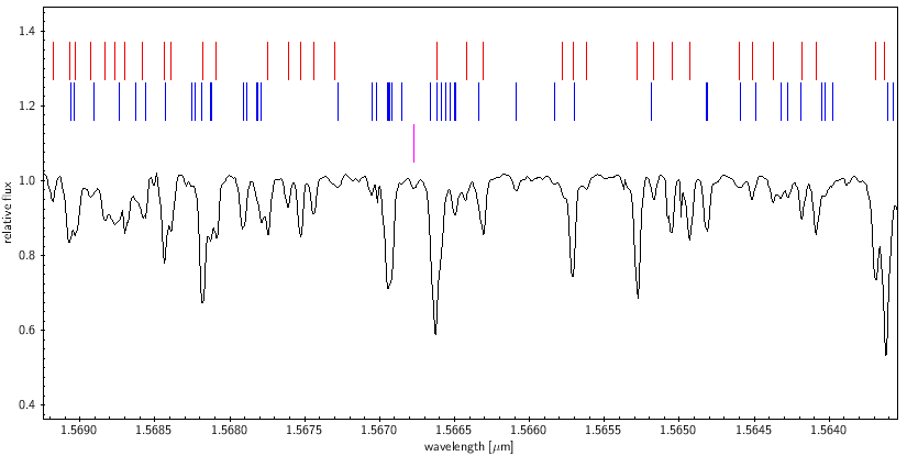
Figure 1: Example section from the 10 Leo spectrum. Identified lines are marked by vertical strokes. The top row (red) corresponds to line identifications in common with the Arcturus atlas. The second row (blue) are identifications attributed based on our model calculations. The single magenta line in the third row indicates an as of yet unidentified feature.

In addition, we identified 9183 lines in 10 Leo with an assigned transition from VALD3 that were not identified in the Arcturus atlas, with 9% of them being isolated lines, meaning that most of these additional identifications are components of line blends. Figure 1 shows an example section with lines identified in our compendium marked. Interestingly, there are 251 lines in 10 Leo with an assignment from the Arcturus atlas that do not show up in the VALD3 database. Furthermore, 292 lines have an identification in the Arcturus atlas, but are missing from the 10 Leo line list. The latter differences are partly due to slight deviations in the covered wavelength range, defect or saturated spectral regions in either of the two spectra, and partly due to different line strengths excluding some lines from being selected.

We compared EWs for all lines identified in both spectra. The largest differences in central depth are noted for Ti I, Sc I, V I, OH, and CO, which show a lower EW in 10 Leo. Some differences between the isotopologues of CO are observed. In 10 Leo, we see stronger lines of ¹²C¹⁷O compared to Arcturus, whereas ¹³C¹⁶O bands are weaker in 10 Leo than in Arcturus. For Fe I, S I, C I, and CN, lines are stronger in 10 Leo. We come back to this point in the context of abundance determination in Sect. 4.

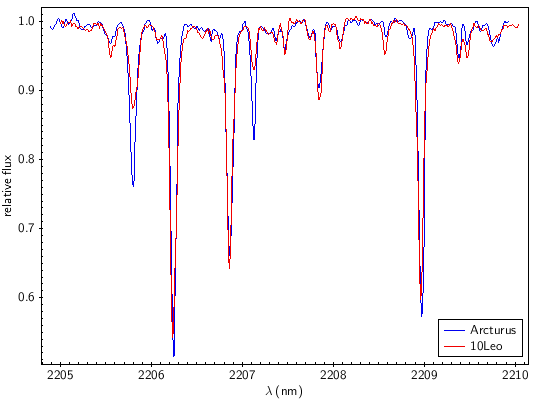
Figure 2: Overlay spectra 10 Leo (red) and Arcturus (blue). See text for details.

Figure 2 shows a typical spectral section with six major lines at 2205.82 nm (Sc I), 2206.24 nm (Na I), 2206.87 nm (Si I), 2207.13 nm (Sc I), 2207.86 nm (Si I), and 2208.97 nm (Na I) as an overlay between 10 Leo and Arcturus. The most obvious difference between the two spectra are the Sc I lines with a significantly enhanced line depth in Arcturus relative to 10 Leo. Minor differences can be seen for the Na I and Si I lines. Table 9 shows the ratios of EWs between the two stars for various metals and molecules.

Table 9: Ratios of EWs (Arcturus and 10 Leo)

species	Ratio	$\#$ evaluated
	Arcturus/10 Leo	lines
CO	1.73 $\pm$ 0.23	35
CH	1.37 $\pm$ 0.31	10
C I	0.76 $\pm$ 0.15	9
CN	0.83 $\pm$ 0.13	171
OH	3.26 $\pm$ 0.43	37
Na I	0.94 $\pm$ 0.03	3
Mg I	1.10 $\pm$ 0.14	20
Al I	1.12 $\pm$ 0.02	10
Si I	0.94 $\pm$ 0.10	51
K I	1.13 $\pm$ 0.13	4
Ca I	1.01 $\pm$ 0.11	22
Sc I	1.90 $\pm$ 0.68	3
Ti I	1.54 $\pm$ 0.12	27
V I	1.69 $\pm$ 0.30	4
Cr I	0.95 $\pm$ 0.10	17
Mn I	1.03 $\pm$ 0.01	7
Fe I	0.96 $\pm$ 0.11	164
Ni I	0.97 $\pm$ 0.10	10
Sr II	1.04 $\pm$ 0.06	3

3 The line compendium

With this paper we publish a complete list of 16 431 lines detected in the CRIRES-POP spectrum of 10 Leo, 91% of which have the line-producing element or molecular species assigned. Combining this list with the fully reduced spectrum from Nicholls et al. (2017) available online, we have provided everything necessary for the production of a comprehensive infrared spectral atlas for 10 Leo. The line lists are made available via machine-readable tables.

The basic structure of this first table is shown in Table 10. A single-letter code in the rightmost column of the table distinguishes various levels of agreement with the VALD3 database and the Arcturus atlas, respectively. The letter code is explained in Table 11. For instance, while lines in category A are found in the spectra of 10 Leo and Arcturus and in the VALD3 database, lines in category B are present in the 10 Leo spectrum and in VALD3, but are not listed in the Arcturus atlas. In addition, we provide an indicator for the level of blending and quality for each line with the following meaning: S=single component, D=two components, T=three components, Q4, Q5,…= 4,5,… components, and X=uncertain continuum level affecting the shape and depth of the line. The latter category accounts for about one-third of all lines. In these cases, the EW given is affected by a higher uncertainty.

Categories C, D, and G indicate lines that are expected from the VALD3-based model or that have been identified in the Arcturus atlas, but do not have a counterpart in the 10 Leo spectrum. We provide separate online tables for each of these cases using a structure similar to Table 10. The lines can be broken down into cases where the line is clearly not visible in 10 Leo (’absent’), and cases where a final decision on the presence is not possible due to noise or missing parts of the 10 Leo spectrum (’inconclusive’). Finally, category G also includes 28 lines where the identification in the Arcturus atlas and from VALD3 is not the same (’IDconflict’). The last row in Table 11 indicates the number of lines in each band without a known identification (category U). These are a subset of the total number of lines in each wavelength band given in the next-to-last row of the table, and are also a subset of the lines in category F. The difference in number between F and U corresponds to the 396 lines we were able to newly assign to molecular and atomic species based on our computations of the expected locations of various, previously unidentified CO lines, and lines from the Peterson & Kurucz (2022) collection of Fe lines.

Table 10: Excerpt from line list for the YJ band

Wave	Absorptance	Equivalent	Wavelength		Species	Transition	Line	Catalogue
number		width	observed	VALD3			quality and	Match
v(cm-1)	1-F	EWO(mA)	WLobs(nm)	WL (nm)	ID		complexity
10387.73	0.196	43	962.67	962.68	CN	CN 1-0Q$\{$1$\}$50.5	D	B
10387.21	0.075	4	962.72	962.72	CN	CN 2-1Q$\{$12$\}$25.5	Q4	B
10387.15	0.096	20	962.73	962.73	CN	CN 2-1P$\{$1$\}$26.5	Q4	A
10386.81	0.103	22	962.76	962.76	CN	CN 1-0R$\{$1$\}$59.5	Q4	A
10386.12	0.127	19	962.82	962.83	Fe I		D	B
10386.06	0.107	2	962.83	962.84	Fe I		D	B
10385.71	0.208	33	962.86	962.87	CN	CN 1-0P$\{$2$\}$42.5	X	A
10385.19	0.290	79	962.91	962.91	Fe I		D	B
10384.85	0.193	41	962.94	962.95	Fe I		D	A
10382.94	0.102	21	963.12	963.12	CN	CN 2-1R$\{$1$\}$43.5	X	A

• The full table is available at the CDS.

Table 11: Number of line matches between 10 Leo (observed), VALD3 (calculated), and Arcturus (observed, Hinkle atlas)

Category	10 Leo	VALD3	Arcturus	YJ	H	K	L	M	sum
A	y	y	y	1367	1375	971	358	1078	5149
B	y	y	n	1941	2958	1984	824	1498	9205
C	n	y	n	1003	2104	1184	702	491	5484
D	n	y	y	9	113	13	3	7	145
E	y	n	y	60	84	13	93	1	251
F	y	n	n	729	324	245	444	84	1826
G	n	n	y	4	82	15	67	7	175
sum				5113	7040	4424	2491	3166	22235
U				436	303	196	415	84	1434

High-quality spectra of stars can be used to determine various spectral parameters for the CO molecule such as the rotational constants B, the ro-vibrational coupling constant $\alpha_{e}$, the centrifugal distortion constant, and the transition energies of the vibrational states of ¹²CO and ¹³CO. Such results are complementary to laboratory measurements that are limited in, for example, temperature. Farrenq et al. (1991) used this approach to derive parameters of the CO molecule from the infrared solar spectrum. The CRIRES-POP 10 Leo spectrum is of sufficient quality to perform a similar study. Resulting values are presented in Table 12 together with the corresponding values from the literature. While there is a good agreement for most constants, we note some differences, most remarkably for $\omega_{e}$ for ¹³CO.

Table 12: Overview of derived molecular constants for $\@element[12]{\mathrm{C}}$O and $\@element[13]{\mathrm{C}}$O (all quantities are in units of cm^-1)

	$\@element[12]{\mathrm{C}}$O		$\@element[13]{\mathrm{C}}$O
Parameter	This work	Literature	This work	Literature
$\omega\textsubscript{e}$	2169.76	2169.756 [1]	2121.37	2141.41 [2]
$\omega\textsubscript{0}$(1-0)	2143.27	2143.27 [3]	2096.07	2096.07 [3]
$\omega\textsubscript{0}$(2-0)	4260.07	4260.06 [3]	4166.83	4166.82 [3]
$\omega\textsubscript{0}$(3-0)	6350.43	6350.44 [3]		6212.32 [3]
$\omega\textsubscript{0}$(3-1)	4207.17	4207.17 [3]	4116.25	4116.25 [3]
$\omega\textsubscript{0}$(4-2)	4154.41	4154.41 [3]	4065.81	4065.81 [3]
Be	1.9309	1.9316 [1]	1.8461
B0	1.9222	1.9225 [3]	1.8372	1.8380 [3]
B1	1.9049	1.9050 [3]	1.8215	1.8216 [3]
B2	1.8872	1.8875 [3]	1.8055	1.8053 [3]
B3	1.8700	1.8700 [3]	1.7890	1.7890 [3]
$\omega\textsubscript{e}$$\chi\textsubscript{e}$	13.236	13.288 [1]	12.640	12.67 [2]
$\alpha\textsubscript{e}$	1.7490E-02	1.7505E-02 [1]	1.6351E-02
De	6.120E-06	6.122E-06 [1]	5.592E-06	5.593E-06 [3]
re(Å)	1.1242	1.1282 [1]

[1] Le Floch (1991); [2] Gendriesch et al. (2009); [3] Coxon & Hajigeorgiou (2004)

• Parameters. $\omega\textsubscript{e}$= harmonic wavenumber; $\omega\textsubscript{0}$=$\Delta$E ($\nu$:1$\leftarrow$0); B_e=equilibrium rotational constant, B₀=rotational constant ($\nu$=0); $\omega\textsubscript{e}$$\chi\textsubscript{e}$=anharmonicity term; r_e(Å)=bond distance; $\alpha\textsubscript{e}$=vibration-rotation interaction constant; D_e=centrifugal distortion constant.

4 Element abundances for 10 Leo and Arcturus

A set of synthetic spectra has been compiled to derive elemental abundances for 10 Leo and Arcturus from the observed high-resolution NIR spectra. In a first step, a line catalogue with respective temperature, log g, and microturbulence was requested from VALD3 based on solar abundances. We then computed a synthetic spectrum on the basis of the Model Atmospheres with Radiative and Convective Scheme (MARCS) structure using the tool Synth3 (Kochukhov, 2012). Differences between the observed and the computed spectrum were analysed for individual elements. Based on this, element abundances in the VALD3 line catalogue file were modified for a new computation of the synthetic spectrum. This iterative process was repeated until a consistent set of abundances for the synthetic spectrum was obtained. To find the best fit, we both minimised the differences for EWs and carried out a visual inspection of an overlay of the observed and synthetic spectrum. Furthermore, the computed and observed EWs of selected lines were compared in unclear cases individually.

Table 13: Abundances for 10 Leo and Arcturus derived from spectral synthesis. Column 2: solar abundances scaled to the metallicity of 10 Leo. Column 3: abundances for 10 Leo derived in this paper by spectral synthesis. Column 4: abundances for Arcturus derived in this paper. Column 5: differences between 10 Leo and Arcturus abundances.

Elementa	Abundances
	Solar scaledb	10 Leo	Arcturus	Leo-Arc
C	-3.52	-3.85$\pm{0.05}$	-4.14	0.29
N	-4.12	-4.05$\pm{0.09}$	-4.37	0.32
O	-3.21	-3.35$\pm{0.09}$	-3.27	-0.08
Na	-5.71	-5.80$\pm{0.02}$	-5.89	0.09
Mg	-4.46	-4.46$\pm{0.17}$	-4.48	0.02
Al	-5.57	-5.40$\pm{0.08}$	-5.41	0.01
Si	-4.49	-4.80$\pm{0.07}$	-4.83	0.03
K	-6.92	-7.00$\pm{0.09}$	-7.09	0.09
Ca	-5.68	-6.00$\pm{0.06}$	-6.08	0.08
Sc	-8.87	-9.00$\pm{0.52}$	-9.10	0.10
Ti	-7.02	-7.30$\pm{0.13}$	-7.39	0.09
V	-8.04	-8.30$\pm{0.31}$	-8.74	0.44
Cr	-6.37	-6.55$\pm{0.07}$	-6.67	0.12
Mn	-6.65	-6.00$\pm{0.10}$	-6.18	0.18
Fe	-4.54	-4.80$\pm{0.17}$	-4.96	0.16
Ni	-5.79	-6.25$\pm{0.08}$	-6.40	0.15
Sr	-9.07	-9.00$\pm{0.05}$	-9.09	0.09

^aOnly neutral lines were used for all elements except for Sr, for which only ionised lines were used. ^bThe solar-scaled abundances are based on the element abundances in the solar photosphere derived by Grevesse & Sauval (1998).

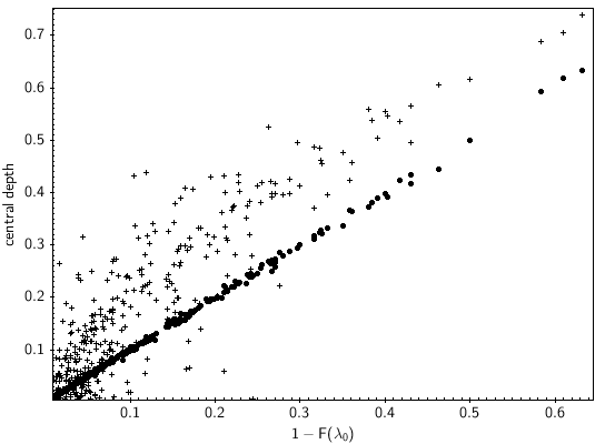
Figure 3: cdepth deduced from the Gaussian fit versus Fe I lines (1-F_{($\lambda\textsubscript{0}$)}). The dots are from individual Gaussian fits to isolated Fe lines in the observed 10 Leo spectrum. The crosses refer to cdepths from the VALD3 extracted stellar calculation for 10 Leo based on solar Fe abundances.

Fig. 3 shows a comparison of the observed and computed central depths for about 340 isolated Fe I lines selected from across the range of the 10 Leo spectrum. Each observed iron line was fitted by a Gaussian curve to derive the respective position, central depth, full width at half maximum (FWHM), and the EW. The central depth from this fit is compared with the observed value of 1-F, where F is the normalised flux at the line centre $\lambda\textsubscript{0}$ (filled circles). The second dataset in this plot (crosses) refers to the same lines with the central depth now derived from the VALD3 stellar extraction model for solar abundances (see Sect. 2.1) with the observed value of 1-F. The Gaussian model provides a good fit to the observed line profiles over the whole range of line strengths studied here. The comparison between the observed and the modelled central depths shows a systematic difference in line depth and considerable scatter around the relation. The systematic difference indicates that 10 Leo has a lower iron abundance than the Sun. The high S/N of the spectrum and the good fit of the observed lines by a Gaussian profile, which indicates a low effect of line blending, suggests that the scatter we see between observed and modelled line depths is only partly due to observational noise, but significantly due to uncertainties in the theoretical line data. Indeed, a number of Fe I lines predicted by the synthetic spectrum could not be observed in the 10 Leo spectrum as discussed in Sect. 2.4 (Tables 8, 16, 17, and 18).

In total, abundances for 17 key elements were determined from the 10 Leo and Arcturus spectra. The third and fourth column of Table 13 reflect the set of abundances for the best fit for 10 Leo and Arcturus, respectively, whereas the second column lists the solar reference values used as the starting point. Abundances for C, N, and O were derived from molecular lines using the approach described in Hinkle et al. (2020). In principle, the abundances of these three elements were altered in each fitting step until a simultaneous fit of the lines of CO, CN, and OH was achieved. The fifth column shows the abundance differences between the two K giants. Abundance uncertainties were derived from the standard deviation of the ratios in EWs between the observed and the synthetic spectrum, and are given in column three of Table 13 for 10 Leo. For Arcturus, the listed abundances come with similar uncertainties. As a K giant, 10 Leo should show an abundance pattern typical for a post first dredge-up object. According to evolutionary models (Karakas & Lattanzio, 2014; Cristallo et al., 2015), we thus expect a reduction of ¹²C and an enhancement of ¹⁴N on the stellar surface. Both trends are clearly visible in Table 13. The C and O abundances are in excellent agreement with the values derived by Luck (2015) from optical spectra. The same authors give abundances for various other elements in 10 Leo, most of them indicating an overabundance compared to the Sun. From our analysis, however, we find most elements to be slightly underabundant compared to the Sun. Solar-like abundances for 10 Leo were reported by da Silva et al. (2015). While error bars both in our analysis and for the literature values do not allow a conclusive comparison, we note that our analysis tends to give a lower mean metallicity for 10 Leo. Tan et al. (2016) independently derived Si abundances from the CRIRES-POP spectrum of 10 Leo and got [Si/Fe]=-0.04$\pm{0.03}$, which is in satisfying agreement with our findings.

Using second overtone lines of ¹²CO and ¹³CO, we derived a ¹²C/¹³C ratio of 22$\pm{8}$ using a curve of growth analysis (Hinkle et al., 2016). To our knowledge, the carbon isotopic ratio had not been measured for this star before. To derive ratios for the main isotopes of oxygen, we used fundamental lines of C¹⁶O, C¹⁷O, and C¹⁸O in the M band. We find ¹⁶O/¹⁷O = 299${}^{-107}_{+241}$ and ¹⁶O/¹⁸O = 345${}^{-125}_{+276}$. These values agree with model expectations for a 2 M_☉ red giant after a first dredge-up and observations for similar stars (Lebzelter et al., 2015; Cristallo et al., 2015).

To estimate the reliability of our abundance determinations for 10 Leo in the absence of a larger set of literature data, we can compare our results for Arcturus, which have been derived in an identical manner, with literature results. We thereby focus on the most recent papers. Very recently measured abundances of Na, Mg, and Al by Lind et al. (2022) agree within the error bars with our findings. That paper also gives abundance corrections for non-local thermodynamic equilibrium (NLTE), which have not been taken into account in our analysis. Fukue et al. (2021) present abundances for C, N, O, Mg, Si, Ca, Ti, Cr, Fe, and Ni, all of which coincide with our findings within 0.1 dex, except for Cr, where Fukue et al. (2021) found an abundance 0.33 dex lower than our result. Further abundances of key elements were presented by Jönsson et al. (2017) and Lomaeva et al. (2019), partly based on the spectrum from the Arcturus atlas. Results for Mg, Ca, Ti, Sc, V, and Ni agree within our error bars. Their O abundance is slightly lower than our value. The abundances from the two mentioned papers coincide with minor differences with the major study by Jofré et al. (2015). The Cr abundance from Lomaeva et al. (2019) agrees with the results from Fukue et al. (2021) and thus significantly differs from our findings. The reason for this difference is not clear. In addition, our Mn abundance is much larger than the value presented in Lomaeva et al. (2019) and in Jofré et al. (2015). Since we also see an outstanding overabundance of this element in 10 Leo compared to the sun, we have to assume the Mn abundances derived in this paper to be potentially erroneous. We aim to understand this discrepancy in a separate study beyond the scope of this paper, which is presenting the line compendium in the CRIRES-POP spectrum of 10 Leo. Except for these two elements, abundances derived for 10 Leo and Arcturus in this paper coincide well with other studies.

5 Summary

The main goal of this paper was to provide a compendium of line identifications for a K giant that is as complete as possible. This includes more than 16 000 lines from molecules and atoms, detected in the pipeline-reduced and fully corrected high-resolution NIR spectrum of the cool star 10 Leo, and their assignment to atomic and molecular species. These results are important for computing synthetic spectra, and abundance determination for evolved stars in general. In addition, the search for lines from neutron capture elements profits from a high degree of completeness and correctness of line lists for Fe and below, including molecular lines. This can assist in determining interfering lines that may completely mask or mimic lines of possible neutron capture elements.

The identification of absorption lines has been done visually with the help of various line lists, stellar extraction from VALD3, and other published sources. Hydrogen and lines from various further elements were identified, including C, Na, Mg, Al, Si, P, S, K, Ca, Sc, Ti, V, Cr, Mn, Fe, Co, Ni, Cu, Zn, Rb, Sr, Y, Zr, Ce, and Dy. Some of these elements, for example Sr, Ce, and Dy, are only detectable in their ionised form.

Molecules such as CO, CN, and OH dominate the spectrum. Absorption lines from $\@element[13]{\mathrm{C}}$O, C$\@element[17]{\mathrm{O,}}$ and C$\@element[18]{\mathrm{O}}$ were easily identified in several bands and with sufficient strengths to determine isotopic ratios. In contrast, absorption lines from $\@element[13]{\mathrm{C}}$N are very weak and only identified for the 0-0 bands. Lines of C$\@element[15]{\mathrm{N}}$ are not detectable in the spectrum.

The comparison between observed and synthetic spectra allowed us to identify a large number of lines that are present in the synthetic spectra but are not observed, and lines that are observed and identified, but not present in the synthetic spectra. The high number of discrepancies reveals the need to improve the spectroscopic data for metals, for example, for Mg and Fe. The $L$ band shows the largest fraction of unidentified lines (29%), and the $M$ band the lowest (6%). Lists of unidentified and missing lines are also part of our line compendium. The quality of the spectrum allows for various spectral parameters for CO to be tested such as the rotational constant, vibrational coupling constant, distortion constant, and transition energies of the vibrational states. We find a good agreement with literature values for ¹²C¹⁶O, but some discrepancies for ¹³C¹⁶O, which require further investigation.

Finally, we have presented abundances for 17 key elements from the CRIRES-POP spectrum of 10 Leo and the FTS spectrum of Arcturus, which are in good agreement with literature values in most cases. This paper complements the CRIRES-POP spectrum of 10 Leo published by Nicholls et al. (2017) providing a complete NIR atlas of this K giant. In comparing it with the Arcturus atlas, metallicity and temperature effects can be studied for individual sections of the 1 to 5 $\mu$m range.

Appendix A Unassigned and unobserved lines

This appendix presents tables of lines present in the 10 Leo spectrum but not assigned to an element or molecule yet (Tables 14 and 15). In addition, we give tables of lines expected to be visible from the VALD3 database, but not observed in the spectra of 10 Leo or Arcturus (Tables 16 to 18). For the YJ band, the corresponding tables can be found in the main part of the paper (Tables 7 and 8).

Table 14: Most intense unassigned lines with an EW¿100 mÅ in the H band and possible contributors

wavelength	EW	possible blends	reference
(nm)	mÅ
1415.75	122	Fe II 1415.74 Ti II 1415.75, Ni II 1415.76 Cs I 1415.78, Cr II 1415.81	(1)
1416.90	161	Co I 1416.90, Mn II 1416.94, V II 1416.92	(1)
1418.00	186
1418.18	187	1418.18 CN 0-1Q(2)13.5, Fe II 1418.17, Ni I 1418.17, Mn i 1418.18,
		V i 1418.18, Sc II 1418.18	(1)
1421.09	102
1421.54	146	Fe II 1421.52, Sc I 1421.51, Mn II 1421.55, Cr I 1421.56	(1)
1424.87	177	Fe I 1421.90	(1)
1425.29	316	Fe I 1425.30 (CN0-1R(2)31.5 subtracted)
1426.37	185	Fe I 1426.39, Ca I 1426.34	(1)
1426.81	134	Ti I 1426.81, Fe I 1426.89	(1)
1427.65	151	Fe II 1427.68, P I 1427.67, C I 1427.64, Ni I 1427.65	(1)
1427.67	121
1427.75	114	Mn I 1427.74, Fe I 1427.74	(1)
1428.38	222	V I 1428.39, 1428.40	(1)
1429.56	142	Mn II 1429.51, (CN 0-1R(1)33.5 subtracted)	(1)
1429.88	103	Mn I 1429.87	(1)
1429.90	146	Sc II 1429.90, V II 1429.91	(1)
1432.89	102	Mn I 1432.88, Fe I 1432.84, Fe II 1432.85	(1)
1434.09	143	Fe II 1434.09, Ti I 1434.09, Si II 1434.07	(1)
1449.79	258	Ti I 1449.79, Fe II 1449.78, Mn II 1449.74,
		V i 1449.76, C I 1449.77, V I 1449.83	(1)
1452.93	230	Fe I 1452.93, Mn I 1452.92,Sc I 1452.94	(1)
1486.66	158	Fe II 1486.61, Si I 1486.69	(1)
1581.45	142	Fe I 1581.45(cdepth 0.037)	(1),(2)
1597.20	251	Fe I 1597.20, Al I triplet 1597.27 (cdepth 0.288)	(1),(2)
1597.73	129	V I 1597.77	(1)
1608.03	187	Ti I 1607.98, Fe I 1608.03 (cdepth 0.048)	(1),(2)
1643.34	135	Ni I 1643.34, Fe II 1643.30	(1)
1696.63	143	Fe I 1696.65 (cdepth 0.090, Cr I 1696.66, Ti I 1696.97	(1)
1707.21	113	Fe I 1707.22 (cdepth 0.055), Fe II 1707.22	(1),(2)
1758.51	164	Co I 1758.47, Cr II 1758.46, Fe I 1758.53	(1),(2)
1774.44	189
1775.22	105	Fe I 1775.22 (cdepth 0.060)	(1)
1794.36	154	1794.40 Cr II 1794.33, P I 1794.34, Si I 1794.38, K I	(1)

(1)Ryabchikova et al. (2015), (2)Hinkle et al. (1995a)

Table 15: Most intense unassigned lines with an EW¿100 mÅ in the K, L, and M band and possible contributors

wavelength	EW	possible blends	referencea
(nm)	mÅ
1978.17	241	strong shoulder on Ca I 1978.22
1979.92	163	Mn I 1979.90, cdepth 0.039	(1)
1986.70	150	strong shoulder on Ca I 1986.76
2009.53	213	Co II 2009.55, Fe II 2009.58, Mn i 2009.48	(1)
2106.54	265	Cr I 2106.56	(1)
2163.17	112	Ti I 2163.24, Fe II 2163.25, V i 2163.12, Ca I 2163.11	(1)
2478.67	157
2499.27	189	Al I 2499.28, cdepth 0.073	(1)
2508.83	224	Ni II 2508.82	(1)
3415.38	381	Ti I 3415.36, Cr I 3415.41	(1)
3416.00	410	Cr I 3416.04	(1)
3542.12	104	Fe II 3542.11	(1)
3544.45	103	V I 3544.45	(1)
3546.79	168	Fe II 3546.77	(1)
3983.61	109
3996.26	103	doublet ( 3996.13 /Co I 3996.23)
3999.95	127	C I 3999.94, Cr II 4000.00	(1)
4006.27	103
4160.42	104	Fe I 4160.31	(2)
4167.66	127
4549.36	393	wavelength correction of -0.11 nm applied
4553.23	188	wavelength correction of -0.11 nm applied
4565.37	393	wavelength correction of -0.08 nm applied, $\@element[13]{\mathrm{C}}$O 2-1R40, C$\@element[18]{\mathrm{O}}$ 2-1R42,
		C$\@element[18]{\mathrm{O}}$ 3-2R27 subtracted
4569.88	426	wavelength correction of -0.03 nm applied, $\@element[13]{\mathrm{C}}$O 2-1R39, C$\@element[17]{\mathrm{O}}$ 2-1R80 subtracted
4572.17	362	C$\@element[17]{\mathrm{O}}$ 3-2R71, C$\@element[18]{\mathrm{O}}$ 4-3R85 subtracted
4574.46	644	CO 2-1R38 subtracted
4576.77	449	Co1 4576.76 $\@element[13]{\mathrm{C}}$O 4-3R74, $\@element[13]{\mathrm{C}}$O 2-1R38 subtracted	(1)
4579.11	356
4580.28	472	Fe II 4580.31, quartet: CO 1-0R10,$\@element[13]{\mathrm{C}}$O 3-2R50, C$\@element[18]{\mathrm{O}}$ 4-3R76, CO 4-3R39 subtracted	(1)
4581.43	190	Fe I 4581.53, $\@element[13]{\mathrm{C}}$O 4-3R70, CO subtracted	(1)
4583.80	109
4595.01	168	Ti I 4594.94	(1)
4595.86	146	CO 3-2R25, CO 3-2R46 subtracted
4625.85	640
4678.84	416	$\@element[13]{\mathrm{C}}$O 4-3R40 subtracted
4682.45	446	$\@element[13]{\mathrm{C}}$O 6-5R85 subtracted
4705.95	299
4726.57	721	CO 1-0P7 subtracted
4748.62	211
4794.91	210	C$\@element[18]{\mathrm{O}}$ 3-2R12 subtracted
4798.53	273	Fe I 4798.55 subtracted
4822.08	177	$\@element[13]{\mathrm{C}}$O 6-5R35 subtracted
4874.71	110	$\@element[13]{\mathrm{C}}$O 9-8R80 subtracted
4882.62	230	C$\@element[17]{\mathrm{O}}$ 1-0P17, CO 10-9R110, $\@element[13]{\mathrm{C}}$O 8-7R49 subtracted
4883.87	500	CO 10-9R57, $\@element[13]{\mathrm{C}}$O 7-6R35, $\@element[13]{\mathrm{C}}$O 9-8R72 subtracted
5023.05	130	blended with $\@element[13]{\mathrm{C}}$O 4-3P8, CO 12-11R56
5087.31	133
5186.19	122	Mn I 5186.29	(1)

(1)Ryabchikova et al. (2015), (2)Hinkle et al. (1995a)

Table 16: Lines with cdepth¿0.10 not present in the observed H-band spectrum.

Wavelength	species	Absorptance(a	Synthetic(b	Wavelength	species	Absorptance(a	Synthetic(b
(nm)	ID	1-F	cdepth	nm	ID	1-F	cdepth
1424.28	Fe I	0.004	0.277	1650.86	Fe I	0.015	0.293
1429.42	Fe I	0.001	0.268	1655.23	Fe I	-0.008	0.115
1432.78	Fe I	-0.006	0.156	1656.12	Fe I	0.058	0.113
1449.58	Fe I	0.008	0.283	1658.59	Fe I	0.015	0.392
1460.77	Fe I	0.006	0.140	1659.43	Si I	0.007	0.133
1461.02	Mg I	-0.030	0.120	1659.77	Ni I	0.023	0.103
1465.34	Mg I	0.088	0.166	1659.78	S I	0.013	0.108
1465.35	Mg I	-0.014	0.119	1663.44	Fe I	0.016	0.247
1481.13	Mg I	0.012	0.123	1664.52	Fe I	0.025	0.162
1486.77	Fe I	0.015	0.129	1664.98	Fe I	0.000	0.115
1487.07	Fe I	0.023	0.203	1665.18	Fe I	-0.002	0.233
1494.12	Fe I	-0.001	0.227	1681.52	Fe I	-0.005	0.103
1501.35	Fe I	-0.001	0.261	1682.26	Fe I	0.035	0.180
1511.03	Fe I	0.090	0.129	1682.62	Fe I	-0.013	0.106
1515.94	Fe I	-0.013	0.242	1684.85	Fe I	0.052	0.258
1519.09	Ti I	-0.018	0.156	1685.77	Ni I	0.008	0.189
1519.94	Ni I	-0.017	0.142	1685.81	Fe I	-0.015	0.179
1521.83	Fe I	-0.015	0.103	1686.31	Fe I	0.011	0.455
1527.57	Fe I	-0.008	0.173	1688.32	Fe I	0.016	0.225
1544.86	Fe I	-0.004	0.366	1688.82	Fe I	0.004	0.175
1544.86	Fe I	0.000	0.285	1700.13	Co I	0.075	0.317
1548.01	Fe I	0.048	0.218	1700.93	Fe I	-0.034	0.143
1548.86	Fe I	-0.002	0.146	1701.50	Mg I	0.018	0.120
1549.03	Fe I	0.008	0.274	1701.74	Fe I	-0.010	0.289
1551.49	Fe I	-0.004	0.344	1702.98	Fe I	0.009	0.244
1559.12	Fe I	0.005	0.201	1704.48	Fe I	-0.004	0.219
1562.20	Fe I	0.026	0.186	1705.23	Fe I	0.017	0.115
1571.26	Ca I	0.061	0.136	1705.75	Fe I	-0.010	0.184
1578.60	Fe I	-0.013	0.142	1717.19	Fe I	-0.012	0.130
1579.38	Fe I	0.028	0.424	1720.38	Fe I	0.012	0.125
1581.24	Si I	0.001	0.189	1728.55	Fe I	-0.002	0.138
1585.84	Fe I	0.037	0.246	1737.59	Fe I	-0.003	0.254
1590.32	Fe I	0.057	0.293	1741.17	Ti I	0.191	0.140
1592.68	Fe I	0.107	0.243	1741.21	Ni I	0.298	0.103
1592.98	Fe I	-0.002	0.110	1745.73	Ca I	-0.003	0.143
1593.30	Fe I	0.027	0.327	1746.39	Fe I	-0.004	0.236
1593.42	Fe I	0.042	0.357	1747.24	Fe I	0.075	0.327
1593.65	Fe I	0.003	0.405	1747.25	Fe I	0.049	0.119
1596.32	Mn I	0.030	0.163	1750.52	Fe I	0.019	0.229
1596.80	Fe I	0.012	0.174	1756.84	Fe I	-0.033	0.142
1596.95	Mn I	0.127	0.212	1758.94	Fe I	0.007	0.294
1597.27	Al I	0.033	0.139	1763.07	Fe I	-0.057	0.233
1600.66	Fe I	0.019	0.213	1769.93	Fe I	-0.005	0.379
1600.78	Fe I	0.022	0.171	1771.42	Fe I	0.006	0.373
1603.01	Fe I	0.017	0.277	1775.37	Co I	-0.002	0.118
1606.18	Fe I	0.019	0.160	1776.51	Fe I	-0.028	0.312
1606.91	Fe I	0.015	0.261	1781.67	Fe I	-0.024	0.133
1608.12	Fe I	-0.002	0.133	1783.24	Fe I	0.008	0.176
1611.55	Fe I	0.016	0.101	1785.08	Fe I	0.200	0.416
1620.68	Fe I	-0.001	0.229	1785.53	Fe I	0.010	0.268
1621.38	Fe I	0.031	0.102	1786.53	Fe I	-0.020	0.410
1623.04	Fe I	0.100	0.413	1786.56	Fe I	0.010	0.132
1623.70	Fe I	0.035	0.210	1786.92	Fe I	0.035	0.193
1624.34	Fe I	-0.008	0.255	1795.42	Ni I	-0.018	0.124
1628.52	Fe I	0.042	0.101	1805.47	Y I	-0.059	0.155
1649.43	Fe I	0.001	0.295	1807.11	Fe I	0.006	0.136
1649.45	Mn I	-0.004	0.273

• ^aobserved (1-F) at wavelength

• ^bVALD3 stellar scaled to solar values

Table 17: Lines with cdepth¿0.10 not present in the observed K-band spectrum.

Wavelength	species	Absorptance(a	Synthetic(b
(nm)	ID	1-F	cdepth
1960.19	Ni I	0.005	0.111
2006.01	Cr I	0.037	0.137
2007.77	Fe I	-0.006	0.223
2009.19	Fe I	-0.005	0.118
2034.51	Fe I	0.000	0.102
2050.11	Ca I	-0.006	0.168
2052.72	Mg I	-0.005	0.356
2052.72	Mg I	-0.003	0.107
2055.31	Fe I	0.015	0.104
2083.06	Fe I	0.004	0.113
2083.91	Mg I	0.085	0.337
2087.28	Mg I	0.000	0.202
2123.95	Mg I	0.001	0.323
2152.80	Fe I	0.011	0.145
2176.70	Mg I	0.010	0.310
2195.73	Fe I	0.000	0.157
2257.78	Fe I	-0.006	0.148
2287.88	Fe I	0.004	0.225
2323.30	Fe I	-0.001	0.160
2329.29	Fe I	0.013	0.200
2350.59	Mg I	0.005	0.137
2351.67	Fe I	0.040	0.247
2369.02	Fe I	-0.011	0.335
2374.31	Mg I	0.042	0.354
2374.31	Mg I	0.079	0.110
2374.33	Mg I	0.040	0.306
2374.33	Mg I	0.016	0.117
2374.33	Mg I	-0.005	0.104
2374.34	Mg I	-0.016	0.304
2384.32	Mg I	0.109	0.288
2389.61	Si I	0.019	0.124
2394.56	Mn I	0.003	0.121
2415.14	Fe I	0.028	0.151
2417.00	Fe I	0.194	0.225
2425.13	Si I	-0.008	0.178
2438.05	Fe I	0.092	0.212
2453.29	Fe I	0.023	0.263
2453.93	Si I	-0.064	0.221
2477.87	Fe I	-0.014	0.110
2502.58	Si I	-0.030	0.121
2507.99	Mg I	0.009	0.168
2508.40	Mg I	0.035	0.205
2508.40	Mg I	0.052	0.144

• ^a observed (1-F) at wavelength

• ^b VALD3 stellar scaled to solar values

Table 18: Lines with cdepth¿0.10 not present in the observed L- and M-band spectra.

Wavelength	species	Absorptance(a	Synthetic(b
(nm)	ID	1-F	cdepth
3473.12	Mg I	-0.005	0.134
3653.47	Mg I	0.021	0.216
3653.48	Mg I	0.018	0.161
3653.51	Mg I	0.006	0.173
3682.04	Fe I	0.005	0.242
3753.46	Mg I	0.007	0.202
3753.48	Mg I	0.002	0.146
3753.51	Mg I	0.005	0.158
3816.43	Mg I	-0.001	0.112
3817.51	Mg I	0.002	0.176
3885.37	Mg I	-0.003	0.191
3885.39	Mg I	0.008	0.135
3885.42	Mg I	-0.002	0.147
3886.01	Fe I	0.000	0.157
3891.67	Fe I	0.007	0.138
3895.44	Fe I	-0.009	0.123
3956.78	Mg I	0.003	0.103
3957.94	Mg I	0.001	0.166
4065.62	Mg I	0.008	0.125
4065.66	Mg I	-0.004	0.138
4093.97	Fe I	0.000	0.161
4114.68	Fe I	0.003	0.190
4120.60	Fe I	-0.001	0.132
4150.98	Mg I	0.014	0.156
4568.96	Si I	-0.013	0.127
4806.30	’CO’	-0.014	0.027
4864.63	Mg I	-0.030	0.107
5013.08	’CO’	-0.009	0.027

• ^a observed (1-F) at wavelength

• ^b VALD3 stellar scaled to solar values