A Convex Framework for Confounding Robust Inference

Abstract

We study policy evaluation of offline contextual bandits subject to unobserved confounders. Sensitivity analysis methods are commonly used to estimate the policy value under the worst-case confounding scenario within a given uncertainty set. However, existing work often resorts to some coarse relaxation of the uncertainty set for the sake of tractability, leading to overly conservative estimation of the policy value. In this paper, we propose a general estimator that provides a sharp lower bound of the policy value using convex programming. The generality of our estimator enables various extensions such as sensitivity analysis using f-divergence, model selection with cross validation and information criterion, and robust policy learning with the sharp lower bound. Furthermore, our estimation method can be reformulated as an empirical risk minimization problem thanks to the strong duality, which enables us to provide strong theoretical guarantees of the proposed estimator using M-estimation techniques.

Keywords: kernel methods, convex optimization, causality, M-estimation, robust optimization.

1 Introduction

The offline contextual bandit, a simple but powerful model for decision-making, finds applications across a spectrum of domains from personalized medical treatment to recommendations and advertisements on online platforms. For the policy evaluation in this setting, the inverse probability weighting (IPW) method (Hirano and Imbens, 2001; Hirano et al., 2003) and its variants are commonly used. These methods rely on the so-called unconfoundedness assumption, presupposing full observability of pertinent variables to exclude any influence from unobserved factors on the action selection and the resulting reward (Rubin, 1974). However, in practice, this unconfoundedness assumption can easily be violated, since often times unobserved confounders are not recorded in the logged data. For instance, consider personalized medicine, where private information such as patients’ financial status is usually not recorded in medical records yet may impact both the choice of treatments and their efficacy. An expensive treatment option may be only available for wealthy patients, and higher financial status may also have a correlation with their health status. In such situations, if the treatment effect of the expensive option depends on the health status of the patients, we can potentially overestimate (or underestimate) the true treatment effect due to this hidden underlying correlation.

To address this, sensitivity analysis offers a solution by establishing a worst-case lower bound on the policy value. This involves defining an uncertainty set encompassing potential confounding situations and evaluating the policy value under the most adverse conditions within this set. Such a worst-case lower bound allows for robust decision-making in the presence of confounding. A wide range of sensitivity models has been studied over the years (Rosenbaum, 2002; Tan, 2006; Rosenbaum et al., 2010; Liu et al., 2013).

The main focus of our paper is the marginal sensitivity model by Tan (2006) and its extensions, which assumes similarity between the observational probability and the true probability of the action given the context in the sense that their odds ratio is not too far from $1$. Recently, Zhao et al. (2019) introduced an elegant algorithm for Tan’s marginal sensitivity analysis using the linear fractional programming, which revitalized the study of this model. They also used the bootstrap method to provide an interpretable estimate of the lower bound. This approach was extended to policy learning in Kallus and Zhou (2018, 2021), where they established a statistical guarantee for confounding robust policy learning through lower bound maximization. Notably, their theoretical analysis included a uniform bound for the estimation error of a class of policies, unlike previous works that only focused on the evaluation of a single policy.

1.1 Motivation

These sensitivity analysis methods rely on algorithms using linear programming with relaxed constraints for their tractability, leading to overly conservative lower bound estimates of the policy value. Such estimates are not necessarily guaranteed to be a consistent estimator of the true lower bound. To obtain a sharp lower bound, conditional moment constraints must be leveraged, which are infinite dimensional linear constraints. Recently, Dorn and Guo (2022) analyzed these constraints and characterized the sharp lower bound of Tan’s marginal sensitivity model with a conditional quantile function of the reward distribution. Using this characterization, they proposed the first tractable algorithm to estimate the sharp lower bound that converges to the true lower bound of the policy value.

In this paper, we address the same problem of sharp estimation from a new perspective. Instead of using the conditional quantile function, we employ the kernel method (Schölkopf et al., 2002), a rich and flexible modeling paradigm in machine learning. With the kernel method, we develop a tractable approximation of the infinite dimensional conditional moment constraints and formulate the sharp lower bound estimation as a convex optimization problem. This formulation is very general and includes the previous sharp estimator by Dorn and Guo (2022) as a special case.

1.2 Contributions

The generality of our estimator expands the horizon of the sensitivity analysis, both in terms of theory and applications.

Our major theoretical contributions stem from the reformulation of the lower bound estimation as an empirical risk minimization using the strong duality. This enables us to leverage the standard proof techniques for M-estimation to derive consistency and asymptotics of our estimator, simplifying our proofs compared to the bespoke proofs in previous works (Kallus and Zhou, 2018, 2021). In particular, we are the first to prove a consistent policy learning guarantee for the sharp lower bound, which parallels the seminal result in Kallus and Zhou (2018, 2021) for the classic unsharp bound. Additionally, we study the property of the specification bias in estimation resulting from our kernel approximation of the conditional moment constraints, and we provide a kernel selection that guarantees zero (or bounded) specification error.

In terms of applications, our kernel formulation is less restrictive compared to the two-stage approach of the previous sharp estimators (Dorn and Guo, 2022; Dorn et al., 2021) and offers possibilities for various extensions, such as generalization of the classic marginal sensitivity model (Tan, 2006) using f-divergence, policy learning with the sharp lower bound, and model selection using the cross validation or the generalized information criterion Konishi and Kitagawa (2008). Furthermore, our estimator can naturally handle both discrete and continuous treatment, setting it apart from conventional unsharp estimators (Tan, 2006; Zhao et al., 2019; Kallus and Zhou, 2018), which are unsuitable for cases involving continuous treatment.

Lastly, we highlight the difference between this paper from an earlier version by the authors (Ishikawa and He, 2023). All the analyses on asymptotic normality and its applications including hypothesis testing and model selection are the novel results of this paper. This paper also provides a more comprehensive study of the consistency and specification bias, by providing the consistent policy learning guarantee for a general Vapnik-Chevonenkis policy class with the sharp lower bound for the first time, and by characterizing the magnitude of the specification bias when the kernel cannot be chosen optimally to achieve zero bias.

1.3 Related works

The idea of using the kernel method to impose constraints has previously been explored in various contexts. To obtain a fair regression model that is guaranteed to discard a sensitive feature, Pérez-Suay et al. (2017) used the kernel Hilbert Schmidt independence criterion and imposed the independence between the sensitive feature and the model’s prediction. In the context of distributionally-robust optimization, the maximum mean discrepancy (Staib and Jegelka, 2019) and the kernel mean embeddings (Zhu et al., 2020) were used to construct an uncertainty set of distribution in the neighborhood of observed data. Aubin-Frankowski and Szabó (2020) imposed shape restrictions to the derivatives of functions by leveraging the differentiability of fitted kernel ridge regression models. Recently, the kernel method has found various novel applications in causal inference, including instrumental variable regression (Singh et al., 2019), negative controls (Singh, 2020; Kallus et al., 2021; Mastouri et al., 2021), and conditional mean squared error minimization for policy evaluation (Kallus, 2018).

Similarly to our paper, Kremer et al. (2022) used the kernel method for parameter estimation of models characterized by conditional moment restrictions. They used the dual representation of the $L^{2}$ norm of the conditional moment to obtain a dual problem. They exploited this dual formulation to obtain theoretical guarantees of parameter estimation. Though we solve a primal problem in this paper, we take great advantage of such a dual problem in our theoretical analysis. Another work that studied conditional moment restriction is Muandet et al. (2020). They consider the hypothesis testing for conditional moment conditions. Their test statistics, maximum moment restriction, is a quadratic form of a kernel matrix which is somewhat similar to the one we use. However, their paper focuses on hypothesis testing while ours focuses on the construction of uncertainty sets.

1.4 Organization of the paper

The remainder of the paper is organized as follows: Section 2 provides the formal formulation of our problem and reviews some of the important results from earlier work. In Section 3, we describe the kernel approximation of the conditional moment constraints and then propose the sharp lower bound estimator of policy value with the approximation. Section 4 studies the theoretical properties of the proposed estimator by reformulating our estimation method by the strong duality. In Section 5 we present our numerical experiments and Section 6 concludes the paper.

2 Backgrounds and Problem Settings

In this section, we present formal definitions for confounded offline contextual bandits and their sensitivity models using partial identification. Given the abundance of notations introduced herein, we offer a list of common notations used throughout the paper in Appendix A.

2.1 Confounded offline contextual bandits

This subsection provides the formal formulation of the confounded offline contextual bandits. Here, we describe our model assumptions in terms of the graphical models (Koller and Friedman, 2009; Pearl, 2009) instead of the potential outcome framework (Rubin, 2005). This is because we find it easier to express our modeling assumptions that accommodate both discrete or continuous action space with the graphical models.

(a) unconfounded case

(b) confounded case

Figure 1: Graphical model of unconfounded and confounded contextual bandit

(Unconfounded) Offline contextual bandits

To clarify our confoundedness assumption, we begin by introducing the unconfounded offline contextual bandits. Let $\mathcal{X}$ and $\mathcal{T}$ be the context space and the action space. The model can be described as the probabilistic model of the three variables: context $X\in\mathcal{X}$, action (or treatment) $T\in\mathcal{T}$, and reward (or outcome) $Y\in\mathbb{R}$. For some unknown base policy $\pi_{\mathrm{base}}(t|x)$, we obtain an offline dataset of these variables from the following data generating process:

$$\begin{array}[]{ll}X&\sim p(x),\\ T|X&\sim\pi_{\mathrm{base}}(t|X),\\ Y|T,X&\sim p(y|T,X).\end{array}$$ (4)

Here, after sampling context $X$ randomly, action $T$ is sampled from a stochastic policy $\pi_{\mathrm{base}}(t|X)$ given context $X$, and reward $Y$ is randomly generated depending on both the context and the action. This model corresponds to the graphical model in Figure 1(a). Under the unconfoundedness assumption, given large enough data, it is possible to identify base policy $\pi_{\mathrm{base}}$ from the observation, as the observational conditional distribution of $T$ given $X$ is equivalent to the distribution of the base policy.

Now, we can consider the offline evaluation of the policy from the observational data. Given new policy $\pi(t|x)$, we are interested in estimating the expectation of reward $Y$ under the following probabilistic model:

$$\begin{array}[]{ll}X&\sim p(x),\\ T|X&\sim\pi(t|X),\\ Y|T,X&\sim p(y|T,X).\end{array}$$ (8)

As the only difference of (8) from (4) is the conditional distribution of action $T$ given context $X$ (i.e., the policy), we introduce simplified notations for these expectations. We will write the expectations of $f(Y,T,X)$ under (4) and (8) as $\mathbb{E}_{T\sim\pi_{\mathrm{base}}(\cdot|X)}[f(Y,T,X)]$ and $\mathbb{E}_{T\sim\pi(\cdot|X)}[f(Y,T,X)]$ respectively. With this notation, we can derive an offline estimate of policy value $V:=\mathbb{E}_{T\sim\pi(\cdot|X)}[Y]$ from relation

$$V(\pi)=\mathbb{E}_{T\sim\pi(\cdot|X)}[Y]=\mathbb{E}_{T\sim\pi_{\mathrm{base}}(\cdot|X)}\left[\left(\frac{\pi(T|X)}{\pi_{\mathrm{base}}(T|X)}\right)Y\right].$$ (9)

The quantity inside the last expectation is unbiased for policy value $V$. Therefore, we can construct the so-called inverse probability weighting (IPW) estimator with data $\{(Y_{i},T_{i},X_{i})\}_{i=1}^{n}$ as

$$\hat{V}_{\mathrm{IPW}}(\pi):=\frac{1}{n}\sum_{i=1}^{n}{\left(\frac{\pi(T_{i}|X_{i})}{\hat{\pi}_{\mathrm{base}}(T_{i}|X_{i})}\right)Y_{i}},$$

where $\hat{\pi}_{\mathrm{base}}$ is estimated from the dataset. A disadvantage of this estimator is the high sensitivity to the estimated inverse of policy probability $1/{\hat{\pi}_{\mathrm{base}}(T_{i}|X_{i})}$. A variation of the estimator called the Hájek estimator is defined as

$$\hat{V}_{\mathrm{H\acute{a}jek}}(\pi):=\frac{\sum_{i=1}^{n}\pi(T_{i}|X_{i})Y_{i}/\hat{\pi}_{\mathrm{base}}(T_{i}|X_{i})}{\sum_{i=1}^{n}1/\hat{\pi}_{\mathrm{base}}(T_{i}|X_{i})}.$$ (10)

Instead of directly using the inverse probability $1/{\hat{\pi}_{\mathrm{base}}(T_{i}|X_{i})}$, the Hájek estimator uses the normalized inverse probability $\frac{1/\hat{\pi}_{\mathrm{base}}(T_{i}|X_{i})}{\frac{1}{n}\sum_{j}1/\hat{\pi}_{\mathrm{base}}(T_{j}|X_{j})}$ so that $\mathbb{E}_{T\sim\pi_{\mathrm{base}}(\cdot|X)}\left[\frac{1}{\pi_{\mathrm{base}}(T|X)}|T=t\right]=1$ is satisfied empirically for all $t\in\mathcal{T}$. Though this estimator tends to be more stable, it is no longer an unbiased estimator of the policy value. However, this estimator is still consistent, and in the context of sensitivity analysis, this estimator is sometimes preferred over the IPW estimator (Zhao et al., 2019; Kallus and Zhou, 2018, 2021; Dorn and Guo, 2022).

Confounded offline contextual bandits

The confounded offline contextual bandits are an extension of the standard offline contextual bandits that have additional unobserved confounding variable $U\in\mathcal{U}$, where $\mathcal{U}$ is the space of confounder $\mathcal{U}$. Unlike other variables $Y$, $T$, and $X$, confounder $U$ is unobservable, and that introduces a confounding effect in the observable data. In confounded offline contextual bandits, the data are generated according to the following model:

$$\begin{array}[]{ll}X,U&\sim p(x,u),\\ T|X,U&\sim\pi_{\mathrm{base}}(t|X,U),\\ Y|T,X,U&\sim p(y|T,X,U),\end{array}$$ (14)

but only $Y$, $T$, and $X$ are observable and policy $\pi_{\mathrm{base}}(t|x,u)$ is unknown. This corresponds to the graphical model in Figure 1(b), where the existence of $U$ is the clear difference from the unconfounded graphical model.

For a better understanding of these variables, let us remember the earlier example of personalized medical treatment. The observational data $\{(Y_{i},T_{i},X_{i})\}_{i=1}^{n}$ corresponds to medical records and they include basic information about patients such as age, sex, and weight, which corresponds to context $X$. Additionally, $T$ and $Y$ are the medical treatment taken by the patients and its outcome. However, some information such as the financial status of the patients is not included in them. Yet, such information can influence the choice of treatment and the effectiveness of the treatment in either direct or indirect manners. Such a variable corresponds to confounder $U$ in our model.

Now, we consider the offline evaluation of policy $\pi$ in confounded contextual bandits, where we need to estimate the expectation of $Y$ under the following model:

$$\begin{array}[]{ll}X,U&\sim p(x,u),\\ T|X,U&\sim\pi(t|X),\\ Y|T,X,U&\sim p(y|T,X,U).\end{array}$$ (18)

Here, we only consider an observable policy $\pi(t|x)$, because it is trivially impossible to evaluate a policy that depends on unobserved variable $U$ only using the offline data.

Indeed, in confounded contextual bandits, offline evaluation of the above observable policy is still impossible without any further assumptions. To explain the reason, let’s consider change of expectations

$$V(\pi)=\mathbb{E}_{T\sim\pi(\cdot|X)}\left[Y\right]=\mathbb{E}_{T\sim\pi_{\mathrm{base}}(\cdot|X,U)}\left[\left(\frac{\pi(T|X)}{\pi_{\mathrm{base}}(T|X,U)}\right)Y\right],$$ (19)

where $\mathbb{E}_{T\sim\pi_{\mathrm{base}}(\cdot|X,U)}[f(Y,T,X,U)]$ and $\mathbb{E}_{T\sim\pi(\cdot|X)}[f(Y,T,X,U)]$ correspond to the expectations of $f(Y,T,X,U)$ under the generative processes (14) and (18). Compared to (9), the inverse probability in (19) has a dependence on unobserved variable $U$. This makes it impossible to construct a consistent estimator such as the IPW estimator and the Hájek estimator in the unconfounded case. As the observable variables are only $Y$, $T$, and $X$, any valid estimator must depend only on them. Ideally, we would like to know conditional expectation of the inverse probability $w(y,t,x):=\mathbb{E}_{T\sim\pi_{\mathrm{base}}(\cdot|X,U)}\left[\frac{1}{\pi_{\mathrm{base}}(T|X,U)}|Y=y,T=t,X=x\right]$. Then, we can construct a valid unbiased and consistent estimator $\hat{V}_{w}:=\frac{1}{n}\sum_{i}w(Y_{i},T_{i},X_{i})\pi(T_{i}|X_{i})Y_{i}$, because

$$V(\pi)=\mathbb{E}_{\mathrm{obs}}\left[\mathbb{E}_{T\sim\pi_{\mathrm{base}}(\cdot|X,U)}\left[\frac{1}{\pi_{\mathrm{base}}(T|X,U)}|Y,T,X\right]\pi(T|X)Y\right].$$ (20)

However, in practice, it is impossible to know $w(y,t,x)$ in the confounded offline contextual bandits.

Hereafter, for simplicity of notation and analysis, we assume that the conditional distribution of reward $Y$ given $T$, $X$, and $U$ is continuous and that it yields a density function $p(y|t,x,u)$ when such assumptions are appropriate. We will also assume that $\pi(T|X,U)>0$ almost surely with respect to (14) so that the inverse probability weights are always well-defined. Additionally, we will use the following simplified notations. To indicate a part of model (14) that can be identified by the offline data, we use $p_{\mathrm{obs}}$ to indicate the observable distribution of (14) so that

$$p_{\mathrm{obs}}(y,t,x)=\int p(y|t,x,u)\pi_{\mathrm{base}}(t|x,u)p(x,u)\,\mathrm{d}u.$$

Similarly, $p_{\mathrm{obs}}(t|x)$ and $p_{\mathrm{obs}}(x)$ will denote the corresponding conditional and marginal distributions, and $\mathbb{E}_{\mathrm{obs}}[f(Y,T,X)]:=\mathbb{E}_{T\sim\pi_{\mathrm{base}}(\cdot|X,U)}[f(Y,T,X)]$ represents the expectation of $f(Y,T,X)$ with respect to $p_{\mathrm{obs}}(y,t,x)$. To represent the empirical average that approximates $\mathbb{E}_{\mathrm{obs}}$, we use $\hat{\mathbb{E}}_{n}$ so that $\hat{\mathbb{E}}_{n}[f(Y,T,X)]:=\frac{1}{n}\sum_{i=1}^{n}f(Y_{i},T_{i},X_{i})$ for any $f(y,t,x)$. Finally, throughout the paper, we assume that we know the true value of $p_{\mathrm{obs}}(t|x)$ in the estimation of the policy value and its lower (or upper) bounds for the sake of simplicity.

2.2 Uncertainty sets of base policies

A practical workaround to the above-mentioned issue is partial identification of the policy value under some reasonable assumption about confounding. More specifically, we first define uncertainty set $\mathcal{E}$ of $\pi_{\mathrm{base}}(t|x,u)$ that we believe to contain all possible base policies underlying the observational data. Then we find infimum policy value $V_{\mathrm{inf}}$ (or supremum $V_{\mathrm{sup}}$) within the uncertainty set as

$$V_{\mathrm{inf}}(\pi):=\inf_{\pi_{\mathrm{base}}\in\mathcal{E}}\mathbb{E}_{T\sim\pi_{\mathrm{base}}(\cdot|X,U)}\left[\left(\frac{\pi(T|X)}{\pi_{\mathrm{base}}(T|X,U)}\right)Y\right].$$ (21)

In the following, we list several types of uncertainty sets for such analysis.

Here, please note that the lower bounds for these uncertainty sets are still intractable, as they involve the expectation with respect to unobserved variable $U$. We will introduce relaxation to these uncertainty sets in the next subsection to obtain a tractable formulation of the lower bound.

Box constraints

The box constraints are the type of uncertainty set that has traditionally been adopted in the sensitivity analysis. They can be expressed as uncertainty set

$$\mathcal{E}_{\mathrm{box}}:=\left\{\pi_{\mathrm{base}}(t|x,u):\begin{array}[]{c}a_{\pi}(t,x)\leq\pi_{\mathrm{base}}(t|x,u)\leq b_{\pi}(t,x)\\ \text{and}\\ \pi_{\mathrm{base}}(\cdot|x,u)\text{ is a proper policy}\end{array}\right\}$$ (22)

for some $a_{\pi}(t,x)$ and $b_{\pi}(t,x)$. This model includes the well-known marginal sensitivity model by Tan (2006) and most of its extensions (Zhao et al., 2019; Kallus and Zhou, 2018; Dorn and Guo, 2022). Tan considered a binary action space and assumed that the odds ratio of observational probability of action $p_{\mathrm{obs}}(t|x)$ and true base policy $\pi_{\mathrm{base}}(t|x,u)$ are not too far from $1$ so that

$$\Gamma^{-1}\leq\frac{p_{\mathrm{obs}}(t|x)(1-\pi_{\mathrm{base}}(t|x,u)}{(1-p_{\mathrm{obs}}(t|x))\pi_{\mathrm{base}}(t|x,u)}\leq\Gamma.$$

As $p_{\mathrm{obs}}(t|x)$ can be identified from the observational data, we can enforce such constraints by choosing $a_{\pi}$ and $b_{\pi}$ in (22) as

$$a_{\pi}(t,x)=\frac{1}{1+\Gamma(1/p_{\mathrm{obs}}(t|x)-1)}\text{ and }b_{\pi}(t,x)=\frac{1}{1+\Gamma^{-1}(1/p_{\mathrm{obs}}(t|x)-1)}.$$ (23)

f-divergence constraint

Here, we introduce a new class of uncertainty sets using the f-divergence. We call the corresponding sensitivity model the f-sensitivity model. Before introducing the new uncertainty set, we first recall the formal definition of f-divergence.

Let $p(t)$ and $q(t)$ be the probability mass function over countable set $\mathcal{T}$ (or the probability density function over $\mathcal{T}\subseteq\mathbb{R}^{d}$ for some $d$ with respect to the Lebesgue measure), and let $f:\mathbb{R}\to\mathbb{R}$ be a convex function satisfying $f(1)=0$. Then, the f-divergence between the distribution of $p(t)$ and $q(t)$ is defined as $D_{f}[p||q]:=\operatorname*{\mathchoice{\ooalign{$\displaystyle\sum$\cr$\displaystyle\int$\cr}}{\ooalign{\raisebox{0.14pt}{\scalebox{0.7}{$\textstyle\sum$}}\cr$\textstyle\int$\cr}}{\ooalign{\raisebox{0.2pt}{\scalebox{0.6}{$\scriptstyle\sum$}}\cr$\scriptstyle\int$\cr}}{\ooalign{\raisebox{0.2pt}{\scalebox{0.6}{$\scriptstyle\sum$}}\cr$\scriptstyle\int$\cr}}}_{\mathcal{T}}f\left(\frac{p(t)}{q(t)}\right)q(t)\,\mathrm{d}t.$ The f-divergence is a rich class of divergence between probability distributions that includes many divergences such as the Kullback-Leibler (KL), squared Hellinger, and Pearson $\chi^{2}$ divergences.

Using the f-divergence, we define a new class of uncertainty set as

$$\mathcal{E}_{f}:=\left\{\pi_{\mathrm{base}}(t|x,u):\begin{array}[]{c}\mathbb{E}_{X,U}\left[D_{f}[p_{\mathrm{obs}}(t|X)||\pi_{\mathrm{base}}(t|X,U)]\right]\leq\gamma\\ \text{and}\\ \pi_{\mathrm{base}}(t|x,u)\text{ is a proper policy}\end{array}\right\},$$ (24)

where the expectation $\mathbb{E}_{X,U}$ can be taken with respect to $p(x,u)$ in both (14) and (18), regardless of the policy. By encoding the proximity of $\pi_{\mathrm{base}}(t|x,u)$ from $p_{\mathrm{obs}}(t|x)$ using the f-divergence instead of the box constraints, we can express our assumption of proximity in a more flexible manner. As we see later, this formulation is also computationally convenient, as the divergence term becomes a simple expectation as

$$\mathbb{E}_{X,U}\left[D_{f}[p_{\mathrm{obs}}(t|X)||\pi_{\mathrm{base}}(t|X,U)]\right]=\mathbb{E}_{T\sim\pi_{\mathrm{base}}(\cdot|X,U)}\left[f\left(\frac{p_{\mathrm{obs}}(T|X)}{\pi_{\mathrm{base}}(t|X,U)}\right)\right].$$ (25)

Indeed, we are not the first to propose the construction of uncertainty sets using the f-divergence in the context of sensitivity analysis. Jin et al. (2022) proposed a similar uncertainty set that approximates the condition

$$D_{f}\left[p\left(Y(1)|X,T=1\right)||p\left(Y(1)|X,T=0\right)\right]\leq\gamma\text{ almost surely},$$

where variable $Y(1)$ is the potential outcome variable for treatment $T=1$ in Rubin’s potential outcome framework (Rubin, 2005) with binary treatment. Under the assumption of unconfoundedness, the potential outcome variable $Y(1)$ must satisfy $Y(1)\perp\!\!\!\perp T|X$, and thus it must satisfy $D_{f}\left[p\left(Y(1)|X,T=1\right)||p\left(Y(1)|X,T=0\right)\right]=0$ almost surely with respect to $p_{\mathrm{obs}}$. Their sensitivity model can be interpreted as a relaxation of this assumption by allowing the violation of it up to $\gamma$. To highlight the difference in modeling paradigm, our f-sensitivity model follows the same modeling framework as Tan (2006), which takes into account the difference between observational policy $p_{\mathrm{obs}}(t|x)$ and underlying confounded policy $\pi_{\mathrm{base}}(t|x,u)$. On the other hand, the model by Jin et al. (2022) considers the distributional shift between observation $Y(1)|X=x,T=1$ and counterfactual $Y(1)|X=x,T=0$, and therefore, their modeling approach is different from Tan (2006) and its extension.

Conditional f-constraint

The above f-sensitivity model can be extended to an even more general case by letting convex function $f$ depend on the values of $T$ and $X$. Let $f:\mathbb{R}\times\mathcal{T}\times\mathcal{X}\to\mathbb{R}$ be a function satisfying that $f_{t,x}(\cdot):=f(\cdot,t,x)$ is convex and $f_{t,x}(1)=0$ for any fixed $t\in\mathcal{T}$ and $x\in\mathcal{X}$. Then, we define the uncertainty set of the conditional f-constraint as

$$\mathcal{E}_{f_{t,x}}:=\left\{\pi_{\mathrm{base}}(t|x,u):\begin{array}[]{c}\mathbb{E}_{T\sim\pi_{\mathrm{base}}(\cdot|X,U)}\left[f_{T,X}\left(\frac{p_{\mathrm{obs}}(T|X)}{\pi_{\mathrm{base}}(T|X,U)}\right)\right]\leq\gamma\\ \text{and}\\ \pi_{\mathrm{base}}(t|x,u)\text{ is a proper policy}\end{array}\right\}.$$ (26)

Clearly, this uncertainty set generalizes f-sensitivity model (24). More interestingly, this model also contains box constraint (22) as the special case. By choosing

$$f_{t,x}(\tilde{w})=I_{[a_{\tilde{w}}(t,x),b_{\tilde{w}}(t,x)]}(\tilde{w})$$ (27)

for $a_{\tilde{w}}(t,x)=p_{\mathrm{obs}}(t|x)/b_{\pi}(t,x)$ and $b_{\tilde{w}}(t,x)=p_{\mathrm{obs}}(t|x)/a_{\pi}(t,x)$, $\mathcal{E}_{f_{t,x}}$ becomes equivalent to the box constraint. Here, $I_{[a,b]}(\tilde{w})$ is a characteristic function of interval $[a,b]$ defined as

$$I_{[a,b]}(\tilde{w}):=\begin{cases}0&\text{ if }\tilde{w}\in[a,b],\\ \infty&\text{otherwise,}\end{cases}.$$

Though we are not particularly interested in the most general form of this uncertainty set in this paper, this uncertainty set turns out to be useful for the systematic treatment of different types of uncertainty sets. Therefore, we will hereafter assume that the uncertainty sets of the inverse probability always have some conditional f-constraint unless otherwise specified, for the sake of theoretical simplicity.

2.3 Relaxation of the uncertainty sets by reparametrization

Having defined the various uncertainty sets, we are now interested in computing lower bound $V_{\mathrm{inf}}$. However, directly solving (21) is often too difficult in practice, so we instead solve a relaxed problem that is more tractable. First, we introduce reparametrization $w(y,t,x)=\mathbb{E}_{T\sim\pi_{\mathrm{base}}(\cdot|X,U)}\left[\frac{1}{\pi_{\mathrm{base}}(T|X,U)}|Y=y,T=t,X=x\right]$. By relaxing the uncertainty set of unknown base policy $\pi_{\mathrm{base}}(t|x,u)$, we can construct an uncertainty set of $w(y,t,x)$ and obtain a convex relaxation of original problem (21).

Without the relaxation, the uncertainty set of base policy $\mathcal{E}_{f_{t,x}}$ can be translated to the uncertainty set of the reparametrized weights as

$$\mathcal{W}_{f_{t,x}}:=\left\{w(y,t,x):\begin{array}[]{c}w(y,t,x)=\mathbb{E}_{T\sim\pi_{\mathrm{base}}(\cdot|X,U)}\left[\frac{1}{\pi_{\mathrm{base}}(T|X,U)}|Y=y,T=t,X=x\right]\\ \text{and}\\ \mathbb{E}_{T\sim\pi_{\mathrm{base}}(\cdot|X,U)}\left[f_{T,X}\left(\frac{p_{\mathrm{obs}}(T|X)}{\pi_{\mathrm{base}}(T|X,U)}\right)\right]\leq\gamma\\ \text{and}\\ \pi_{\mathrm{base}}(t|x,u)\text{ is a proper policy}\end{array}\right\}.$$ (28)

Using (20), we can obtain the lower bound as

$$V_{\mathrm{inf}}(\pi)=\inf_{w\in\mathcal{W}_{f_{t,x}}}\mathbb{E}_{\mathrm{obs}}\left[w(Y,T,X)\pi(T|X)Y\right].$$ (29)

This uncertainty set requires that the expectation of the conditional f-divergence is bounded and that the base policy $\pi_{\mathrm{base}}(t|x,u)$ is proper. However, in practice, both conditions are intractable. Therefore, we will consider the relaxation of these conditions.

Relaxation of the conditional f-constraint

Let us consider the first condition of (28) on conditional f-divergence. With Jensen’s inequality, we have

$$\mathbb{E}_{T\sim\pi_{\mathrm{base}}(\cdot|X,U)}\left[f_{T,X}\left(\frac{p_{\mathrm{obs}}(T|X)}{\pi_{\mathrm{base}}(T|X,U)}\right)\right]\geq\mathbb{E}_{T\sim\pi_{\mathrm{base}}(\cdot|X,U)}\left[f_{T,X}\left(\mathbb{E}\left[\frac{p_{\mathrm{obs}}(T|X)}{\pi_{\mathrm{base}}(T|X,U)}|Y,T,X\right]\right)\right].$$ (30)

Therefore, we can relax condition $\mathbb{E}_{T\sim\pi_{\mathrm{base}}(\cdot|X,U)}\left[f_{T,X}\left(\frac{p_{\mathrm{obs}}(T|X)}{\pi_{\mathrm{base}}(T|X,U)}\right)\right]\leq\gamma$ in (24) to

$$\mathbb{E}_{\mathrm{obs}}\left[f_{T,X}\left(p_{\mathrm{obs}}(T|X)w(Y,T,X)\right)\right]\leq\gamma.$$ (31)

Here, we must emphasize that the above constraint is convex with respect to $w(y,t,x)$. This convexity translates to the empirical version of the above constraint, which enables us to estimate the lower bound by solving convex programming.

Additionally, when $f_{t,x}$ does not depend on $t$ and $x$, there is a simple trick to ensure that the left hand side of (31) is non-negative. By imposing $\mathbb{E}_{\mathrm{obs}}\left[p_{\mathrm{obs}}(T|X)w(Y,T,X)\right]=1$, we can guarantee $0=f(1)=f\left(\mathbb{E}_{\mathrm{obs}}\left[p_{\mathrm{obs}}(T|X)w(Y,T,X)\right]\right)\leq\mathbb{E}_{\mathrm{obs}}\left[f\left(p_{\mathrm{obs}}(T|X)w(Y,T,X)\right)\right]$ due to Jensen’s inequality. In the numerical experiments, we observed that this helps to obtain a more stable implementation of the f-sensitivity model.

Relaxation of the distributional constraints

Now we consider the relaxation of the second condition in (28) that $\pi_{\mathrm{base}}(t|x,u)$ is a proper distribution, which is equivalent to

$$\operatorname*{\mathchoice{\ooalign{$\displaystyle\sum$\cr$\displaystyle\int$\cr}}{\ooalign{\raisebox{0.14pt}{\scalebox{0.7}{$\textstyle\sum$}}\cr$\textstyle\int$\cr}}{\ooalign{\raisebox{0.2pt}{\scalebox{0.6}{$\scriptstyle\sum$}}\cr$\scriptstyle\int$\cr}}{\ooalign{\raisebox{0.2pt}{\scalebox{0.6}{$\scriptstyle\sum$}}\cr$\scriptstyle\int$\cr}}}_{\mathcal{T}}\pi_{\mathrm{base}}(t^{\prime}|x,u)\,\mathrm{d}t^{\prime}=1\text{ and }\pi_{\mathrm{base}}(t|x,u)\geq 0\text{ for any }t\in\mathcal{T},x\in\mathcal{X},\text{ and }u\in\mathcal{U}.$$ (32)

These constraints have traditionally been relaxed to the constraint used in the Hájek estimator. However, there also exists a tighter relaxation called conditional moment constraints, which we employ in our work. In the following, we present these two types of relaxation.

ZSB constraints

When action space $\mathcal{T}$ is discrete and finite, a well-known relaxation of (32) is

$$\mathbb{E}_{\mathrm{obs}}[\mathbbm{1}_{T=t}w(Y,T,X)]=1\text{ for any }t\in\mathcal{T}$$ (33)

and

$$w(y,t,x)\geq 0\text{ for any }y\in\mathcal{Y},t\in\mathcal{T},\text{ and }x\in\mathcal{X},$$ (34)

where $\mathbbm{1}$ denotes the indicator function for event $A$. The first constraint corresponds to the constraint used in the construction of Hájek estimator (10). Following the naming convention in Dorn and Guo (2022), we will call these constraints the ZSB constraints after the authors of Zhao et al. (2019). Condition (33) can be obtained as

$$\mathbb{E}_{\mathrm{obs}}[w(Y,T,X)\mathbbm{1}_{T=t}] =\mathbb{E}_{T\sim\pi_{\mathrm{base}}(\cdot|X,U)}\left[\frac{\mathbbm{1}_{T=t}}{\pi_{\mathrm{base}}(T|X,U)}\right]$$

$$=\mathbb{E}_{X,U}\left[\int_{\mathbb{R}}\sum_{t^{\prime}\in\mathcal{T}}\left(\frac{\mathbbm{1}_{t^{\prime}=t}}{\pi_{\mathrm{base}}(t^{\prime}|X,U)}\right)p(y|t^{\prime},X,U)\pi_{\mathrm{base}}(t^{\prime}|X,U)\,\mathrm{d}y\right]$$

$$=\mathbb{E}_{X,U}\left[\sum_{t^{\prime}\in\mathcal{T}}\mathbbm{1}_{t^{\prime}=t}\int_{\mathbb{R}}p(y|t^{\prime},X,U)\,\mathrm{d}y\right]=1,$$

and the non-negativity condition is trivial from the definition of $w(y,t,x)$.

To simplify the treatment of the non-negativity condition, we hereafter assume that the non-negativity condition is already imposed by conditional f-constraint (31) so that $f_{t,x}(u)=\infty$ for any $u<0$. This can be assumed without loss of generality because for any conditional-f constraint $\mathbb{E}_{\mathrm{obs}}[f_{t,x}(w(Y,T,X)p_{\mathrm{obs}}(T|X)]\leq\gamma$, we can consider a new f-constraint $\mathbb{E}_{\mathrm{obs}}[\tilde{f}_{t,x}(w(Y,T,X)p_{\mathrm{obs}}(T|X)]\leq\gamma$ for $\tilde{f}_{t,x}(v)=f_{t,x}(v)+I_{[0,\infty)}(v)$.

Combining the above with the relaxation of the conditional f-constraint as in (31), the following uncertainty set with the ZSB constraints can be defined:

$$\mathcal{W}_{f_{t,x}}^{\mathrm{ZSB}}:=\left\{w(y,t,x):\begin{array}[]{c}\mathbb{E}_{X,U}\left[f_{T,X}\left(p_{\mathrm{obs}}(T|X)w(Y,T,X)\right)\right]\leq\gamma\\ \text{and}\\ \mathbb{E}_{\mathrm{obs}}[\mathbbm{1}_{T=t}w(Y,T,X)]=1\text{ for any }t\in\mathcal{T}\end{array}\right\}.$$ (35)

This uncertainty set has been traditionally adopted by many works such as Tan (2006); Zhao et al. (2019); Kallus and Zhou (2018, 2021). For this uncertainty set, associated lower bound

$$V_{\mathrm{inf}}^{\mathrm{ZSB}}(\pi):=\inf_{w\in\mathcal{W}^{\mathrm{ZSB}}}\mathbb{E}_{\mathrm{obs}}\left[w(Y,T,X)\pi(T|X)Y\right]$$ (36)

can be consistently approximated straightforwardly. By approximating the expectations by empirical average, we get a linear program with parameter $\boldsymbol{w}=(w_{1},\ldots,w_{n})^{T}=\left(w(Y_{1},T_{1},X_{1}),\ldots,w(Y_{n},T_{n},X_{n})\right)^{T}$,

$$\hat{V}_{\mathrm{inf}}^{\mathrm{ZSB}}(\pi):=\min_{\boldsymbol{w}\in\hat{\mathcal{W}}_{f_{t,x}}^{\mathrm{ZSB}}}\hat{\mathbb{E}}_{n}[w(Y,T,X)\pi(T|X)Y]$$ (37)

where

$$\hat{\mathcal{W}}_{f_{t,x}}^{\mathrm{ZSB}}:=\left\{\boldsymbol{w}:\begin{array}[]{c}\hat{\mathbb{E}}_{n}[f_{T,X}\left(p_{\mathrm{obs}}(T|X)w(Y,T,X)\right)]\leq\gamma\\ \text{and}\\ \hat{\mathbb{E}}_{n}[\mathbbm{1}_{T=t}w(Y,T,X)]=1\text{ for all }t\in\mathcal{T}\end{array}\right\}.$$ (38)

Here we should note that (37) is not exactly the estimator used in Zhao et al. (2019) and its recent extensions. Instead, they replaced the objective by $\frac{\sum_{t\in\mathcal{T}}\hat{\mathbb{E}}_{n}[w(Y,T,X)\pi(T|X)Y|T=t]}{\hat{\mathbb{E}}_{n}[w(Y,T,X)|T=t]}$ to normalize the weight per treatment and used the linear fractional programming to solve their version of the problem.

Conditional moment constraints

Now, we introduce the sharper constraints that we leverage in our work. We relax constraint (32) as conditional moment constraints

$$\mathbb{E}_{\mathrm{obs}}[w(Y,T,X)|T=t,X=x]\cdot p_{\mathrm{obs}}(t|x)=1\text{ for any }t\in\mathcal{T}\text{ and }x\in\mathcal{X}$$ (39)

plus non-negativity constraint (34), which we assumed is already included in conditional f-constraint (31). Unlike ZSB constraints (33), this relaxation no longer requires the assumption that action space $\mathcal{T}$ is discrete and finite. We can check the validity of this relaxation from

$$\mathbb{E}_{\mathrm{obs}} [w(Y,T,X)|T=t,X=x]\cdot p_{\mathrm{obs}}(t,x)$$

$$=\mathbb{E}_{\mathrm{obs}}\left[\mathbb{E}_{T\sim\pi_{\mathrm{base}}(\cdot|X,U)}\left[\frac{1}{\pi_{\mathrm{base}}(T|X,U)}|Y,T,X\right]|T=t,X=x\right]\cdot p_{\mathrm{obs}}(t,x)$$

$$=\mathbb{E}_{T\sim\pi_{\mathrm{base}}(\cdot|X,U)}\left[\frac{1}{\pi_{\mathrm{base}}(T|X,U)}|T=t,X=x\right]\cdot p_{\mathrm{obs}}(t,x)$$

$$=\operatorname*{\mathchoice{\ooalign{$\displaystyle\sum$\cr$\displaystyle\int$\cr}}{\ooalign{\raisebox{0.14pt}{\scalebox{0.7}{$\textstyle\sum$}}\cr$\textstyle\int$\cr}}{\ooalign{\raisebox{0.2pt}{\scalebox{0.6}{$\scriptstyle\sum$}}\cr$\scriptstyle\int$\cr}}{\ooalign{\raisebox{0.2pt}{\scalebox{0.6}{$\scriptstyle\sum$}}\cr$\scriptstyle\int$\cr}}}_{\mathcal{U}}\frac{1}{\pi_{\mathrm{base}}(t|x,u)}p_{\pi_{\mathrm{base}}}(u|t,x)\,\mathrm{d}u\cdot p_{\mathrm{obs}}(t,x)$$

$$=\operatorname*{\mathchoice{\ooalign{$\displaystyle\sum$\cr$\displaystyle\int$\cr}}{\ooalign{\raisebox{0.14pt}{\scalebox{0.7}{$\textstyle\sum$}}\cr$\textstyle\int$\cr}}{\ooalign{\raisebox{0.2pt}{\scalebox{0.6}{$\scriptstyle\sum$}}\cr$\scriptstyle\int$\cr}}{\ooalign{\raisebox{0.2pt}{\scalebox{0.6}{$\scriptstyle\sum$}}\cr$\scriptstyle\int$\cr}}}_{\mathcal{U}}\frac{1}{\pi_{\mathrm{base}}(t|x,u)}p_{\pi_{\mathrm{base}}}(t,x,u)\,\mathrm{d}u$$

$$=\operatorname*{\mathchoice{\ooalign{$\displaystyle\sum$\cr$\displaystyle\int$\cr}}{\ooalign{\raisebox{0.14pt}{\scalebox{0.7}{$\textstyle\sum$}}\cr$\textstyle\int$\cr}}{\ooalign{\raisebox{0.2pt}{\scalebox{0.6}{$\scriptstyle\sum$}}\cr$\scriptstyle\int$\cr}}{\ooalign{\raisebox{0.2pt}{\scalebox{0.6}{$\scriptstyle\sum$}}\cr$\scriptstyle\int$\cr}}}_{\mathcal{U}}p(x,u)\,\mathrm{d}u=p_{\mathrm{obs}}(x)$$

and the fact that $p_{\mathrm{obs}}(t|x)=p_{\mathrm{obs}}(t,x)/p_{\mathrm{obs}}(x)$. Here, $p_{\pi_{\mathrm{base}}}(t,x,u)$ and $p_{\pi_{\mathrm{base}}}(u|t,x)$ denote the joint and conditional distribution of $T$, $X$, and $U$ under confounded contextual bandits model (14). We can again combine these conditional moment constraints (CMC) with relaxed conditional f-constraint (31) to obtain

$$\mathcal{W}_{f_{t,x}}^{\mathrm{CMC}}:=\left\{w(y,t,x):\begin{array}[]{c}\mathbb{E}_{X,U}\left[f_{T,X}\left(p_{\mathrm{obs}}(T|X)w(Y,T,X)\right)\right]\leq\gamma\\ \text{and}\\ \mathbb{E}_{\mathrm{obs}}[w(Y,T,X)|T=t,X=x]\cdot p_{\mathrm{obs}}(t|x)=1\text{ for any }t\in\mathcal{T}\text{ and }x\in\mathcal{X}\end{array}\right\}$$ (40)

and its corresponding lower bound

$$V_{\mathrm{inf}}^{\mathrm{CMC}}(\pi):=\inf_{w\in\mathcal{W}^{\mathrm{CMC}}}\mathbb{E}_{\mathrm{obs}}\left[w(Y,T,X)\pi(T|X)Y\right].$$ (41)

Naturally, for these uncertainty sets, one can show inclusion relations $\mathcal{W}_{f_{t,x}}\subseteq\mathcal{W}^{\mathrm{CMC}}_{f_{t,x}}\subseteq\mathcal{W}^{\mathrm{ZSB}}_{f_{t,x}}$. The former inclusion follows from the definition of $\mathcal{W}^{\mathrm{CMC}}_{f_{t,x}}$. We can show the latter inclusion by taking the (conditional) expectation of conditional moment constraints (39) with respect to $p_{\mathrm{obs}}(x|t)$ to obtain ZSB constraint (33). Assuming that the true base policy is contained in original sensitivity model $\mathcal{E}_{f_{t,x}}$, these inclusion relations imply $V\geq V_{\mathrm{inf}}\geq V_{\mathrm{inf}}^{\mathrm{CMC}}\geq V_{\mathrm{inf}}^{\mathrm{ZSB}}$.

One important question to ask here is under what kind of setting second equality $V_{\mathrm{inf}}=V_{\mathrm{inf}}^{\mathrm{CMC}}$ holds so that the lower bound of the conditional moment constraints is tight. Surprisingly, recent work by Dorn and Guo (2022) showed that this equality holds for average treatment effect estimation with Tan’s marginal sensitivity model (Tan, 2006). They showed that there exists minimizer $w^{*}(y,t,x)$ of $\mathrm{ATE}(w):=\mathbb{E}_{\mathrm{obs}}[w(Y,T,X)\mathbbm{1}_{T=1}Y]-\mathbb{E}_{\mathrm{obs}}[w(Y,T,X)\mathbbm{1}_{T=0}Y]$, which is realizable so that there exists $p(y|t,x,u)$, $\pi_{\mathrm{base}}(t|x,u)$, and $p(x,u)$ that is compatible with any $p_{\mathrm{obs}}(y,t,x)$ and minimizer $w^{*}(y,t,x)$. However, they did not provide any realizability results for more general settings discussed in this paper such as the evaluation of general policy, non-binary action spaces, and general box and f-constraints, and it is an open question we could not address in this paper.

3 Kernel Conditional Moment Constraints

Here, we introduce an empirical approximation of conditional moment constraints (39) using the kernel method (Schölkopf et al., 2002). The key idea is to estimate the conditional moment $\mathbb{E}_{\mathrm{obs}}[w(Y,T,X)p_{\mathrm{obs}}(T|X)|T=t,X=x]$ with the kernel ridge regression. By constraining the estimated conditional moment to be close to $1$, we impose the conditional moment constraints to empirical inverse probability weight $\boldsymbol{w}=(w_{1},\ldots,w_{n})^{T}=\left(w(Y_{1},T_{1},X_{1}),\ldots,w(Y_{n},T_{n},X_{n})\right)^{T}$.

3.1 Estimating conditional expectation by kernel ridge regression

We begin by formally formulating the idea of using kernel ridge regression for conditional moment constraints. Let us introduce a kernel $k:(\mathcal{T}\times\mathcal{X})\times(\mathcal{T}\times\mathcal{X})\to\mathbb{R}$ with associated reproducing kernel Hilbert space (RKHS) $\mathcal{H}$ of functions $h:\mathcal{T}\times\mathcal{X}\to\mathbb{R}$, inner product $\langle\cdot,\cdot\rangle_{\mathcal{H}}$, and norm $\|\cdot\|_{\mathcal{H}}$. Let us further introduce re-parametrization $e(y,t,x):=p_{\mathrm{obs}}(t|x)w(y,t,x)-1$, so that conditional moment constraints (39) can be written as

$$\mathbb{E}_{\mathrm{obs}}[e(Y,T,X)|T=t,X=x]=0\text{ \ \ for any \ \ }t\in\mathcal{T}\text{ and }x\in\mathcal{X}.$$ (42)

Then, using the kernel ridge regression, one can estimate conditional expectation $g(t,x):=\mathbb{E}_{\mathrm{obs}}[e(Y,T,X)|T=t,X=x]$ as

$$\hat{g}=\arg\min_{g\in\mathcal{H}}\hat{\mathbb{E}}_{n}|g(T,X)-e(Y,T,X)|^{2}+\sigma^{2}\|g\|_{\mathcal{H}}^{2}.$$

for some $\sigma^{2}>0$. The above problem yields an analytical solution, and we can get

$$\hat{\boldsymbol{g}}=K(K+\sigma^{2}I_{n})^{-1}\boldsymbol{e}$$

for $\hat{\boldsymbol{g}}:=\left(\hat{g}(T_{1},X_{1}),\ldots,\hat{g}(T_{n},X_{n})\right)^{T}$ and $\boldsymbol{e}:=\left(e(Y_{1},T_{1},X_{1}),\ldots,e(Y_{n},T_{n},X_{n})\right)^{T}$. Here, $K$ denotes the kernel matrix so that $K_{i,j}=k((T_{i},X_{i}),(T_{j},X_{j}))$ and $I_{n}$ is the identity matrix of order $n$. To impose the conditional moment constraints, we will consider the constraint

$$\hat{\boldsymbol{g}}\approx\boldsymbol{0}$$ (43)

However, we cannot impose the exact equality in the above, as the exact equality would imply

$$K(K+\sigma^{2}I_{n})^{-1}\boldsymbol{e}=\boldsymbol{0}.$$ (44)

Assuming that $K$ is full rank, this implies only solution $\boldsymbol{e}=\boldsymbol{0}$, which is equivalent to $\boldsymbol{w}=\boldsymbol{1}/\boldsymbol{p}_{\mathrm{obs},T|X}$. For this only solution, the resulting policy value estimator is exactly the confounded IPW estimator (19). To overcome this issue, we will consider a low-rank approximation of (44) to enforce it at reasonable strength.

3.2 Low-rank approximation

It is well known that kernel ridge regression suppresses the smaller eigenvalues of the kernel matrix, and therefore, its low-rank approximation can be fairly accurate when the dominant eigenvalues are preserved. This motivates us to replace the original kernel ridge regression with the above low-rank linear regression to obtain a low-rank version of constraint (44). With the kernel principal component analysis (PCA) (Schölkopf et al., 1997), we can obtain feature vectors $\boldsymbol{\varphi}^{\mathrm{KPCA}}(t,x):=\left(\varphi^{\mathrm{KPCA}}_{1}(t,x),\ldots,\varphi^{\mathrm{KPCA}}_{D}(t,x)\right)^{T}$ that approximates the original kernel as $k\left((t,x),(t^{\prime},x^{\prime})\right)\approx{\boldsymbol{\varphi}^{\mathrm{KPCA}}(t,x)}^{T}\boldsymbol{\varphi}^{\mathrm{KPCA}}(t^{\prime},x^{\prime})$. Then, we can approximate the solution of the kernel ridge regression as $e^{*}(t,x)={\boldsymbol{\beta}^{*}}^{T}\boldsymbol{\varphi}^{\mathrm{KPCA}}(t,x)$, where

$$\beta^{*} =\arg\min_{\boldsymbol{\beta}\in\mathbb{R}^{D}}\mathbb{E}_{\mathrm{obs}}\left|e-{\boldsymbol{\varphi}^{\mathrm{KPCA}}}^{T}\boldsymbol{\beta}\right|^{2}$$ (45)

$$=\left(\mathbb{E}_{\mathrm{obs}}\left[\boldsymbol{\varphi}^{\mathrm{KPCA}}{\boldsymbol{\varphi}^{\mathrm{KPCA}}}^{T}\right]\right)^{-1}\mathbb{E}_{\mathrm{obs}}\left[\boldsymbol{\varphi}^{\mathrm{KPCA}}e\right].$$ (46)

By enforcing constraint $\boldsymbol{\beta}^{*}=\boldsymbol{0}$ so that resulting estimator $g^{*}(t,x)$ becomes a zero function, we get orthogonality condition,

$$\mathbb{E}_{\mathrm{obs}}[e(Y,T,X)\varphi^{\mathrm{KPCA}}_{d}(T,X)]=0$$

for any $d=1,\ldots,D$. The same conclusion can be obtained for the empirical version of the constraints, by exchanging expectation operator $\mathbb{E}_{\mathrm{obs}}$ with empirical expectation operator $\hat{\mathbb{E}}_{\mathrm{obs}}$. Therefore, we now have $D$ linear constraints instead of the overly tight full-rank constraint, which makes the conditional moment constraints tractable.

Indeed, constraint (42) implies orthogonality condition $\mathbb{E}_{\mathrm{obs}}[e(Y,T,X)\psi(T,X)]=0$ for any function $\psi(t,x)$. Therefore, we generalize the orthogonality conditions above to any collection of functions $\{\psi_{d}(t,x)\}_{d=1}^{D}$ and define the kernel conditional moment constraints (KCMC) for the population as

$$\mathrm{KCMC}\stackrel{{\scriptstyle\text{def}}}{{\Leftrightarrow}}\mathbb{E}_{\mathrm{obs}}[e(Y,T,X)\psi_{d}(T,X)]=0\text{ \ \ for any \ \ }d=1,\ldots,D.$$ (47)

Analogously, the empirical version of the KCMC is also defined by replacing $\mathbb{E}_{\mathrm{obs}}$ with $\hat{\mathbb{E}}_{n}$.

Finally, combining the KCMC approximation (47) and relaxed conditional f-constraint (31), we can define the uncertainty set

$$\mathcal{W}^{\mathrm{KCMC}}_{f_{t,x}}=\left\{w(y,t,x):\begin{array}[]{c}\mathbb{E}_{\mathrm{obs}}[f_{T,X}(w(Y,T,X)p_{\mathrm{obs}}(T|X))]\leq\gamma\\ \text{and}\\ \mathbb{E}_{\mathrm{obs}}[\left(w(Y,T,X)p_{\mathrm{obs}}(T|X)-1\right)\psi_{d}]=0\text{ \ for any }d=1,\ldots,D.\end{array}\right\}$$ (48)

and the associated estimator of the lower bound with the KCMC as

$$V_{\mathrm{inf}}^{\mathrm{KCMC}}(\pi)=\inf_{w\in\mathcal{W}^{\mathrm{KCMC}}_{f_{t,x}}}\mathbb{E}_{\mathrm{obs}}[w(Y,T,X)\pi(T|X)Y].$$ (49)

Likewise, we use its empirical version and define the KCMC estimator as

$$\hat{V}_{\mathrm{inf}}^{\mathrm{KCMC}}(\pi)=\inf_{\boldsymbol{w}\in\hat{\mathcal{W}}^{\mathrm{KCMC}}_{f_{t,x}}}\hat{\mathbb{E}}_{n}[w(Y,T,X)\pi(T|X)Y],$$ (50)

where

$$\hat{\mathcal{W}}^{\mathrm{KCMC}}_{f_{t,x}}=\left\{w(y,t,x):\begin{array}[]{c}\hat{\mathbb{E}}_{n}[f_{T,X}(w(Y,T,X)p_{\mathrm{obs}}(T|X))]\leq\gamma\\ \text{and}\\ \hat{\mathbb{E}}_{n}[\left(w(Y,T,X)p_{\mathrm{obs}}(T|X)-1\right)\psi_{d}]=0\text{ \ for any }d=1,\ldots,D\end{array}\right\}.$$ (51)

4 Theoretical Analysis

In this section, we study the property of lower bound estimation of the policy value with the kernel conditional moment constraints. We begin the analysis of the KCMC estimator by deriving the convex dual of the above problems and characterizing their minimizers. Then, we study the specification error of the KCMC lower bound $\left|V^{\mathrm{CMC}}_{\mathrm{inf}}-V^{\mathrm{KCMC}}_{\mathrm{inf}}\right|$. We provide a condition on the orthogonal function set $\{\psi_{d}(t,x)\}_{d=1}^{D}$ under which the specification error becomes zero. We also provide an upper bound of the specification error when the condition for no specification error is violated. Next, we show the consistency of the KCMC estimator in policy evaluation, by showing the equivalence of the KCMC estimator with a standard M-estimator. We further prove consistency guarantees for policy learning with the KCMC estimator, in the cases of a concave policy class and the Vapnik-Chevonenkis policy class. Lastly, we derive the asymptotic normality of the KCMC estimator and discuss its application to the construction of a confidence interval and model selection.

Before further discussion, we introduce several simplifications of the notations. We omit subscripts of $\mathcal{W}_{f_{t,x}}^{\mathrm{CMC}}$, $\mathcal{W}_{f_{t,x}}^{\mathrm{KCMC}}$, $\hat{\mathcal{W}}_{f_{t,x}}^{\mathrm{KCMC}}$ and $\mathbb{E}_{\mathrm{obs}}$, unless they are unclear from the context. We also introduce $r(y,t,x)=\left(\frac{\pi(t|x)}{p_{\mathrm{obs}}(t|x)}\right)\cdot y$ and reparametrization $\tilde{w}(y,t,x)=p_{\mathrm{obs}}(t|x)w(y,t,x)$.

Furthermore, we introduce the subgradient and the Fenchel conjugate here, as we will make heavy use of them in this section. The subgradient of convex function $f$ is represented by $\partial f$. When we apply the addition operator to the subgradient, it represents the Minkowski sum. Other operations to the subgradient such as multiplication are similarly defined. The Fenchel conjugate of $f:\mathbb{R}\to\mathbb{R}$ is defined as $f^{*}(v):=\sup_{u}\{uv-f(u)\}$, and it has a few important properties. The Fenchel conjugate is always convex because the supremum of a family of convex functions is convex. Additionally, there exists maximizer $u^{*}$ that solves $f^{*}(v)=\max_{u}\left\{vu-f(u)\right\}$ and it satisfies

$$u^{*}\in\partial f^{*}(v)$$ (52)

if $f$ is closed and convex. Function $f$ is closed and convex if its epigraph $\mathrm{epi}(f):=\{(u,t):u\in\mathrm{dom}(f),\ f(u)\leq t\}$ is closed and convex, and these conditions are satisfied in our problem. A more thorough treatment of the subgradient and the Fenchel conjugate can be found in (Boyd et al., 2004).

4.1 Characterization of the solution

In this subsection, we derive explicit formulae for the minimizers that give three lower bounds $V_{\mathrm{inf}}^{\mathrm{CMC}}$, $V_{\mathrm{inf}}^{\mathrm{KCMC}}$, and $\hat{V}_{\mathrm{inf}}^{\mathrm{KCMC}}$, which are

$$\begin{split}w^{*}_{\mathrm{CMC}}&=\arg\min_{w\in\mathcal{W}^{\mathrm{CMC}}}\mathbb{E}[w(Y,T,X)\pi(T|X)Y],\\ w^{*}_{\mathrm{KCMC}}&=\arg\min_{w\in\mathcal{W}^{\mathrm{KCMC}}}\mathbb{E}[w(Y,T,X)\pi(T|X)Y],\\ \hat{w}_{\mathrm{KCMC}}&=\arg\min_{w\in\hat{\mathcal{W}}^{\mathrm{KCMC}}}\hat{\mathbb{E}}_{n}[w(Y,T,X)\pi(T|X)Y].\end{split}$$ (53)

Here, we know that these problems have minimizers because the above problems are minimizations of linear objectives under convex constraints. Furthermore, we know that the strong duality holds for the above convex optimizations, as their feasibility sets have a non-empty relative interior, satisfying Slater’s constraint qualification. Using these properties, we obtain the following lemma:

Lemma 1 (Characterization of solutions).

Let $w^{*}_{\mathrm{CMC}}$, $w^{*}_{\mathrm{KCMC}}$, and $\hat{w}_{\mathrm{KCMC}}$ be defined as in (53). Then, there exist function $\eta_{\mathrm{CMC}}:\mathcal{T}\times\mathcal{X}\to\mathbb{R}$, vectors $\eta_{\mathrm{KCMC}},\eta_{\mathrm{KCMC}}^{\prime}\in\mathbb{R}^{D}$, and constants $\eta_{f},\eta_{f}^{\prime},\eta_{f}^{\prime\prime}>0$ such that

$$w^{*}_{\mathrm{CMC}}(y,t,x) \in\left(\frac{1}{p_{\mathrm{obs}}(t|x)}\right)\partial f_{t,x}^{*}\left(\frac{\eta_{\mathrm{CMC}}(t,x)-r(y,t,x)}{\eta_{f}}\right),$$ (54)

$$w^{*}_{\mathrm{KCMC}}(y,t,x) \in\left(\frac{1}{p_{\mathrm{obs}}(t|x)}\right)\partial f_{t,x}^{*}\left(\frac{{\eta_{\mathrm{KCMC}}}^{T}\boldsymbol{\psi}(t,x)-r(y,t,x)}{\eta_{f}^{\prime}}\right),$$ (55)

$$\hat{w}_{\mathrm{KCMC}}(y,t,x) \in\left(\frac{1}{p_{\mathrm{obs}}(t|x)}\right)\partial f_{t,x}^{*}\left(\frac{{\eta_{\mathrm{KCMC}}^{\prime}}^{T}\boldsymbol{\psi}(t,x)-r(y,t,x)}{\eta_{f}^{\prime\prime}}\right).$$ (56)

Proof  See below.  

Characterization of $w^{*}_{\mathrm{CMC}}$

By using the strong duality, we can transform the original problem for $V_{\mathrm{inf}}^{\mathrm{CMC}}$ as

$$V_{\mathrm{inf}}^{\mathrm{CMC}} =\inf_{w\in\mathcal{W}^{\mathrm{CMC}}}\mathbb{E}[\tilde{w}(Y,T,X)r(Y,T,X)]$$ (57)

$$=\inf_{\tilde{w}}\sup_{\begin{subarray}{c}\eta_{\mathrm{CMC}}:\mathcal{T}\times\mathcal{X}\to\mathbb{R},\\ \eta_{f}\geq 0\end{subarray}}\mathbb{E}[\tilde{w}r]-\mathbb{E}\left[\eta_{\mathrm{CMC}}(T,X)\mathbb{E}[\tilde{w}-1|T,X]\right]+\eta_{f}\left(\mathbb{E}[f_{T,X}(\tilde{w})]-\gamma\right)$$ (58)

$$=\sup_{\begin{subarray}{c}\eta_{\mathrm{CMC}}:\mathcal{T}\times\mathcal{X}\to\mathbb{R},\\ \eta_{f}\geq 0\end{subarray}}\inf_{\tilde{w}}\mathbb{E}[\tilde{w}r]-\mathbb{E}\left[\eta_{\mathrm{CMC}}(T,X)(\tilde{w}-1)\right]+\eta_{f}\left(\mathbb{E}[f_{T,X}(\tilde{w})]-\gamma\right)$$ (59)

$$=\sup_{\begin{subarray}{c}\eta_{\mathrm{CMC}}:\mathcal{T}\times\mathcal{X}\to\mathbb{R},\\ \eta_{f}>0\end{subarray}}-\eta_{f}\gamma+\mathbb{E}[\eta_{\mathrm{CMC}}]-\eta_{f}\mathbb{E}\left[\sup_{\tilde{w}}\left\{\left(\frac{\eta_{\mathrm{CMC}}-r}{\eta_{f}}\right)\tilde{w}-f_{T,X}(\tilde{w})\right\}\right]$$ (60)

$$=\sup_{\begin{subarray}{c}\eta_{\mathrm{CMC}}:\mathcal{T}\times\mathcal{X}\to\mathbb{R},\\ \eta_{f}>0\end{subarray}}-\eta_{f}\gamma+\mathbb{E}[\eta_{\mathrm{CMC}}]-\eta_{f}\mathbb{E}\left[f_{T,X}^{*}\left(\frac{\eta_{\mathrm{CMC}}-r}{\eta_{f}}\right)\right],$$ (61)

assuming that optimal $\eta_{f}$ is positive. This assumption does not hold only when conditional f-constraint (31) is not tight so that $\mathbb{E}\left[f_{T,X}(\tilde{w})\right]<\gamma$, for instance, in the case of the box constraints (27). In such cases, inner supremum is reached for $\eta_{f}=0$ and we have a more simple dual

$$V_{\mathrm{inf}}^{\mathrm{CMC}} =\sup_{\eta_{\mathrm{CMC}}:\mathcal{T}\times\mathcal{X}\to\mathbb{R}}\inf_{\tilde{w}}\mathbb{E}[\tilde{w}r]-\mathbb{E}\left[\eta_{\mathrm{CMC}}(T,X)(\tilde{w}-1)\right]$$ (62)

$$=\sup_{\eta_{\mathrm{CMC}}:\mathcal{T}\times\mathcal{X}\to\mathbb{R}}\mathbb{E}[\eta_{\mathrm{CMC}}]-\mathbb{E}\left[f_{T,X}^{*}\left(\eta_{\mathrm{CMC}}-r\right)\right].$$ (63)

Hereafter, we consider the cases where $\eta_{f}>0$ for simplicity of the proofs, unless their extension to the cases where $\eta_{f}=0$ is non-trivial.

Now, as primal solution $w^{*}_{\mathrm{CMC}}$ must satisfy the Karush-Kuhn-Tucker (KKT) conditions, we can take the maximizers of (61) as $\eta_{f}^{*}$ and $\eta_{\mathrm{CMC}}^{*}(t,x)$. Using property (52) of the Fenchel conjugate, we can obtain solution form of $w^{*}_{\mathrm{CMC}}$

$$w^{*}_{\mathrm{CMC}}(y,t,x)\in\left(\frac{1}{p_{\mathrm{obs}}(t|x)}\right)\partial f_{t,x}^{*}\left(\frac{\eta_{\mathrm{CMC}}^{*}(t,x)-r(y,t,x)}{\eta_{f}^{*}}\right),$$ (64)

which proves (54) . Here, factor $1/p_{\mathrm{obs}}(t|x)$ in front of the subgradient appears because of reparametrization $\tilde{w}(y,t,x)=p_{\mathrm{obs}}(t|x)w(y,t,x)$. The maximizers of the dual solutions $\eta_{f}^{*}$ and $\eta_{\mathrm{CMC}}^{*}$ can be characterized by taking the stationary conditions as

$$0 \in\partial_{\eta_{f}}\left(-\eta_{f}\gamma+\mathbb{E}[\eta_{\mathrm{CMC}}]-\eta_{f}\mathbb{E}\left[f_{T,X}^{*}\left(\frac{\eta_{\mathrm{CMC}}-r}{\eta_{f}}\right)\right]\right)$$ (65)

$$=-\gamma-\mathbb{E}\left[f_{T,X}^{*}\left(\frac{\eta_{\mathrm{CMC}}-r}{\eta_{f}}\right)\right]+\mathbb{E}\left[\left(\frac{\eta_{\mathrm{CMC}}-r}{\eta_{f}}\right)\cdot\partial f_{T,X}^{*}\left(\frac{\eta_{\mathrm{CMC}}-r}{\eta_{f}}\right)\right]$$ (66)

and

$$0 \in\partial_{\eta_{\mathrm{CMC}}}\left(-\eta_{f}\gamma+\mathbb{E}[\eta_{\mathrm{CMC}}]-\eta_{f}\mathbb{E}\left[f_{T,X}^{*}\left(\frac{\eta_{\mathrm{CMC}}-r}{\eta_{f}}\right)\right]\right)$$ (67)

$$=1-\mathbb{E}\left[\partial f_{T,X}^{*}\left(\frac{\eta_{\mathrm{CMC}}-r}{\eta_{f}}\right)|T=t,X=x\right],$$ (68)

where we used the functional gradient on measure $p_{\mathrm{obs}}$ in the second subgradient condition.

For general choice of $f_{t,x}$, it is difficult to derive analytical expressions for solutions $\eta_{f}^{*}$ and $\eta^{*}_{\mathrm{CMC}}$, as well as $w^{*}_{\mathrm{CMC}}$. However, we can actually obtain their explicit expressions in the case of the box constraints.

Example 1 (Solutions for box constraints).

Let us consider the box constraints corresponding to (27) of the conditional f-constraint. Here, for notational simplicity, we omit the subscript of $a_{\tilde{w}}$ and $b_{\tilde{w}}$. For example, we will simply write $f_{t,x}(\tilde{w})=I_{[a(t,x),b(t,x)]}(\tilde{w})$. Then, for this choice of function $f_{t,x}$, we can derive its conjugate and its subgradient as

$$f_{t,x}^{*}(v)=\begin{cases}a(t,x)v&\text{ if \ \ }v<0,\\ 0&\text{ if \ \ }v=0,\\ b(t,x)v&\text{ if \ \ }v>0,\end{cases}$$ (69)

and

$$\partial f_{t,x}^{*}(v)=\begin{cases}a(t,x)&\text{ if \ \ }v<0,\\ [a(t,x),b(t,x)]&\text{ if \ \ }v=0,\\ b(t,x)&\text{ if \ \ }v>0.\end{cases}$$ (70)

Substituting the above expression of $\partial f_{t,x}^{*}$ in the first order condition of (63), we can derive more explicit expression

$$1 =\mathbb{E}\left[\partial f_{T,X}^{*}\left(\eta_{\mathrm{CMC}}-r\right)|T=t,X=x\right]$$ (71)

$$=\mathbb{P}(r<\eta_{\mathrm{CMC}}(t,x))\cdot b(t,x)+\mathbb{P}(r=\eta_{\mathrm{CMC}}(t,x))\cdot[a(t,x),b(t,x)]+\mathbb{P}(r>\eta_{\mathrm{CMC}}(t,x))\cdot a(t,x).$$ (72)

Here, we used the box constraints’ property $a(t,x)\leq 1\leq b(t,x)$, which follows from the requirement that $f_{t,x}$ must satisfy $f_{t,x}(1)=0$ for any $t\in\mathcal{T}$ and $x\in\mathcal{X}$. Assuming that the conditional distribution of $r(Y,T,X)$ given $T=t$ and $X=x$ yields continuous distribution for any $t\in\mathcal{T}$ and $x\in\mathcal{X}$, the second subgradient condition becomes

$$1=\mathbb{P}(r\leq\eta_{\mathrm{CMC}}(t,x))\cdot b(t,x)+\mathbb{P}(r>\eta_{\mathrm{CMC}}(t,x))\cdot a(t,x).$$ (73)

This implies that $\mathbb{P}(r\leq\eta_{\mathrm{CMC}}(t,x))=\frac{1-a(t,x)}{b(t,x)-a(t,x)}=:\tau(t,x)$, and therefore,

$$\eta^{*}_{\mathrm{CMC}}(t,x)=\left(\frac{\pi(t|x)}{p_{\mathrm{obs}}(t|x)}\right)Q(t,x),$$ (74)

where $Q(t,x)$ was defined as the $\tau(t,x)$-quantile of the conditional distribution of $Y$ given $T=t$ and $X=x$. From this dual solution, the primal solution can also be recovered using (54) as

$$w^{*}_{\mathrm{CMC}}(y,t,x)=\begin{cases}b(t,x)&\text{ if \ \ }y\leq Q(t,x),\\ a(t,x)&\text{ otherwise}.\end{cases}$$ (75)

Characterization of $w^{*}_{\mathrm{KCMC}}$

Now, we derive the characterization of $w^{*}_{\mathrm{KCMC}}$. Let $\boldsymbol{\psi}(t,x)=\left(\psi_{1}(T,X),\ldots,\psi_{D}(T,X)\right)^{T}$. We can use exactly the same technique as the above and reach a similar characterization of the solution as

$$V_{\mathrm{inf}}^{\mathrm{KCMC}} =\inf_{w\in\mathcal{W}^{\mathrm{KCMC}}}\mathbb{E}[\tilde{w}(Y,T,X)r(Y,T,X)]$$ (76)

$$=\inf_{\tilde{w}}\sup_{\begin{subarray}{c}\eta_{\mathrm{KCMC}}\in\mathbb{R}^{D},\\ \eta_{f}\geq 0\end{subarray}}\mathbb{E}[\tilde{w}r]-\mathbb{E}\left[(\tilde{w}-1){\eta_{\mathrm{KCMC}}}^{T}\boldsymbol{\psi}\right]+\eta_{f}\left(\mathbb{E}[f_{T,X}(\tilde{w})]-\gamma\right)$$ (77)

$$=\sup_{\begin{subarray}{c}\eta_{\mathrm{KCMC}}\in\mathbb{R}^{D},\\ \eta_{f}\geq 0\end{subarray}}\mathbb{E}[\tilde{w}r]-\mathbb{E}\left[(\tilde{w}-1){\eta_{\mathrm{KCMC}}}^{T}\boldsymbol{\psi}\right]+\eta_{f}\left(\mathbb{E}[f_{T,X}(\tilde{w})]-\gamma\right)$$ (78)

$$=\sup_{\begin{subarray}{c}\eta_{\mathrm{KCMC}}\in\mathbb{R}^{D},\\ \eta_{f}>0\end{subarray}}-\eta_{f}\gamma+{\eta_{\mathrm{KCMC}}}^{T}\mathbb{E}[\boldsymbol{\psi}]-\eta_{f}\mathbb{E}\left[\sup_{\tilde{w}}\left\{\left(\frac{{\eta_{\mathrm{KCMC}}}^{T}\boldsymbol{\psi}-r}{\eta_{f}}\right)\tilde{w}-f_{T,X}(\tilde{w})\right\}\right]$$ (79)

$$=\sup_{\begin{subarray}{c}\eta_{\mathrm{KCMC}}\in\mathbb{R}^{D},\\ \eta_{f}>0\end{subarray}}-\eta_{f}\gamma+{\eta_{\mathrm{KCMC}}}^{T}\mathbb{E}[\boldsymbol{\psi}]-\eta_{f}\mathbb{E}\left[f_{T,X}^{*}\left(\frac{{\eta_{\mathrm{KCMC}}}^{T}\boldsymbol{\psi}-r}{\eta_{f}}\right)\right].$$ (80)

Now, using the maximizers of dual problem (80) $\eta_{f}^{*}$ and $\eta_{\mathrm{KCMC}}^{*}$, we can obtain a characterization of $w^{*}_{\mathrm{KCMC}}$ as

$$w^{*}_{\mathrm{KCMC}}(y,t,x)\in\left(\frac{1}{p_{\mathrm{obs}}(t|x)}\right)\partial f^{*}\left(\frac{{\eta_{\mathrm{KCMC}}^{*}}^{T}\boldsymbol{\psi}(t,x)-r(y,t,x)}{\eta_{f}^{*}}\right),$$ (81)

which proves (55).

Now we study the characterization of dual solutions $\eta_{f}^{*}$ and $\eta_{\mathrm{CMC}}^{*}$. Again, we take the stationary conditions as

$$0 \in\partial_{\eta_{f}}\left(-\eta_{f}\gamma+{\eta_{\mathrm{KCMC}}}^{T}\mathbb{E}[\boldsymbol{\psi}]-\eta_{f}\mathbb{E}\left[f_{T,X}^{*}\left(\frac{{\eta_{\mathrm{KCMC}}}^{T}\boldsymbol{\psi}-r}{\eta_{f}}\right)\right]\right)$$ (82)

$$=-\gamma-\mathbb{E}\left[f_{T,X}^{*}\left(\frac{{\eta_{\mathrm{KCMC}}}^{T}\boldsymbol{\psi}-r}{\eta_{f}}\right)\right]+\mathbb{E}\left[\left(\frac{{\eta_{\mathrm{KCMC}}}^{T}\boldsymbol{\psi}-r}{\eta_{f}}\right)\cdot\partial f_{T,X}^{*}\left(\frac{{\eta_{\mathrm{KCMC}}}^{T}\boldsymbol{\psi}-r}{\eta_{f}}\right)\right]$$ (83)

and

$$0 \in\partial_{\eta_{\mathrm{KCMC}}}\left(-\eta_{f}\gamma+{\eta_{\mathrm{KCMC}}}^{T}\mathbb{E}[\boldsymbol{\psi}]-\eta_{f}\mathbb{E}\left[f_{T,X}^{*}\left(\frac{{\eta_{\mathrm{KCMC}}}^{T}\boldsymbol{\psi}-r}{\eta_{f}}\right)\right]\right)$$ (84)

$$=\mathbb{E}\left[\boldsymbol{\psi}\left(1-\partial f_{T,X}^{*}\left(\frac{{\eta_{\mathrm{KCMC}}}^{T}\boldsymbol{\psi}-r}{\eta_{f}}\right)\right)|T=t,X=x\right].$$ (85)

Characterization of $\hat{w}_{\mathrm{KCMC}}$

Again, using the same techniques, we can derive the characterization of $\hat{w}_{\mathrm{KCMC}}$. By exchanging $\mathbb{E}$ with $\hat{\mathbb{E}}_{n}$ in the proof for $w^{*}_{\mathrm{KCMC}}$ above and writing the maximizers of dual problem

$$\sup_{\begin{subarray}{c}\eta_{\mathrm{KCMC}}\in\mathbb{R}^{D},\\ \eta_{f}>0\end{subarray}}-\eta_{f}\gamma+{\eta_{\mathrm{KCMC}}}^{T}\hat{\mathbb{E}}_{n}[\boldsymbol{\psi}]-\eta_{f}\hat{\mathbb{E}}_{n}\left[f_{T,X}^{*}\left(\frac{{\eta_{\mathrm{KCMC}}}^{T}\boldsymbol{\psi}-r}{\eta_{f}}\right)\right].$$ (86)

as $\hat{\eta}_{f}$ and $\hat{\eta}_{\mathrm{KCMC}}$, we get

$$\hat{w}_{\mathrm{KCMC}}(y,t,x)\in\left(\frac{1}{p_{\mathrm{obs}}(t|x)}\right)\partial f_{t,x}^{*}\left(\frac{{{}\hat{\eta}_{\mathrm{KCMC}}}^{T}\boldsymbol{\psi}(t,x)-r(y,t,x)}{{\hat{\eta}}_{f}}\right),$$ (87)

which proves (56).

4.2 Specification error

Using the above characterization of the solutions, we can find a condition under which the specification error of estimator $\hat{V}_{\mathrm{inf}}^{\mathrm{KCMC}}(\pi)$ becomes zero, i.e., $\left|V_{\mathrm{inf}}^{\mathrm{KCMC}}(\pi)-V_{\mathrm{inf}}^{\mathrm{CMC}}(\pi)\right|=0$.

Theorem 2 (Zero specification error).

Let $\eta^{*}_{\mathrm{CMC}}(t,x)$ be the solution of dual problem (61) for $V_{\mathrm{inf}}^{\mathrm{CMC}}(\pi)$. Then, if

$$\eta_{\mathrm{CMC}}^{*}\in\mathrm{span}\left(\{\psi_{1},\ldots,\psi_{D}\}\right),$$ (88)

we have

$$V_{\mathrm{inf}}^{\mathrm{CMC}}(\pi)=V_{\mathrm{inf}}^{\mathrm{KCMC}}(\pi).$$ (89)

Proof  Take $\eta^{*}_{f}$ such that $\left(\eta^{*}_{\mathrm{CMC}}(t,x),\ \eta^{*}_{f}\right)$ is the solution of dual problem (61) for $V_{\mathrm{inf}}^{\mathrm{CMC}}$. Then, we can take multiplier $\eta_{\mathrm{KCMC}}^{*}$ that satisfies $\eta_{\mathrm{CMC}}^{*}={\eta_{\mathrm{KCMC}}^{*}}^{T}\boldsymbol{\psi}$. Now, we can see that dual problem (80) for $V_{\mathrm{inf}}^{\mathrm{KCMC}}$ can be considered as the restricted version of dual problem (61) for $V_{\mathrm{inf}}^{\mathrm{CMC}}$ where $\eta_{\mathrm{CMC}}$ is constrained to the subspace spanned by $\{\psi_{1},\ldots,\psi_{D}\}$. Therefore, as restricted solution $\left(\eta^{*}_{\mathrm{KCMC}},\ \eta^{*}_{f}\right)$ achieves the same value as the solution of the non-restricted problem, it is clearly a solution of restricted problem (80). Finally, owing to the strong duality, we can calculate the values of $V_{\mathrm{inf}}^{\mathrm{CMC}}$ and $V_{\mathrm{inf}}^{\mathrm{KCMC}}$ by the values of the dual problems, which implies $V_{\mathrm{inf}}^{\mathrm{CMC}}=V_{\mathrm{inf}}^{\mathrm{KCMC}}$.  

Interestingly, with the above result, we can derive quantile balancing constraint (90) for the previously proposed sharp estimator by Dorn and Guo (2022).

Example 2 (Derivation of quantile balancing estimator (Dorn and Guo, 2022)).

Let us consider the same box constraints as Example 1. For this problem, we know the analytical form of the dual solution, $\eta^{*}_{\mathrm{CMC}}(t,x)=\left(\frac{\pi(t|x)}{p_{\mathrm{obs}}(t|x)}\right)Q(t,x)$. Therefore, we can take $D=1$ and set $\psi_{1}(t,y)=\left(\frac{\pi(t|x)}{p_{\mathrm{obs}}(t|x)}\right)Q(t,x)$ to meet condition (88) in Theorem 2 to obtain the kernel conditional moment constraint with no specification error. Therefore, we can solve (41) in the case of the box constraints as

$$V_{\mathrm{inf}}^{\mathrm{CMC}}(\pi)=\min_{a_{w}(t,x)\leq w(y,t,x)\leq b_{w}(t,x)}\mathbb{E}_{\mathrm{obs}}[w(Y,T,X)\pi(T|X)Y]$$

subject to

$$\mathbb{E}_{\mathrm{obs}}[w(Y,T,X)\pi(T|X)Q(T,X)]=\mathbb{E}_{\mathrm{obs}}\left[\left(\frac{\pi(T|X)}{p_{\mathrm{obs}}(T|X)}\right)Q(T,X)\right],$$ (90)

where $Q(t,x)$ denotes the $\tau(t,x)$-quantile of the conditional distribution of $Y$ given $T=t$ and $X=x$ for $\tau(t,x):=\frac{1/p_{\mathrm{obs}}(t|x)-a_{w}(t,x)}{b_{w}(t,x)-a_{w}(t,x)}$. In the case of marginal sensitivity model (23) by Tan (2006), the expression for $\tau(t,x)$ can be simplified as $\tau(x)=\frac{1}{1+\Gamma}$, and therefore, $Y$ can be estimated by the standard quantile regression. The quantile balancing (QB) estimator introduced by Dorn and Guo (2022) relies on this property and estimates the sharp lower bound by solving the empirical version of the above problem with quantile estimate $\hat{Q}(t,x)$ obtained by the quantile regression.

In addition to showing that their two-stage estimator can be considered a special case of the KCMC estimator, we can also argue that the KCMC estimator can be sharper than the quantile balancing estimator. For that purpose, we pick an equivalent choice of feature sets for the KCMC estimator and the QB estimator. When function set $\{\psi_{d}(t,x)\}_{d=1}^{D}$ is used by the KCMC estimator, we can choose $\left\{\left(\frac{p_{\mathrm{obs}}(t|x)}{\pi(t|x)}\right)\psi_{d}(t,x)\right\}_{d=1}^{D}$ as the feature of the linear quantile regression so that $\eta_{\mathrm{KCMC}}^{*}$. Then, when the solution of the quantile regression is $\hat{Q}(t,x)={\hat{\eta}_{\mathrm{KCMC}}}^{T}\boldsymbol{\psi}(t,x)$, the QB estimator becomes as tight as the KCMC estimator. However, in general, the solution of the quantile regression may not coincide $\hat{\eta}_{\mathrm{KCMC}}$ even at an infinite sample limit, since the objective of the quantile regression is not equivalent to the dual objective of the KCMC estimator.

As our estimator generalizes the previous work, our estimator overcomes some drawbacks of the quantile balancing estimators. As discussed in Section 1, the quantile balancing estimator cannot handle policy learning and the f-constraint. Policy learning is also difficult with the quantile balancing estimator because taking the derivative with respect to policy requires differentiability of the solution of the above linear programming with respect to parameter $\hat{Q}$. Moreover, the quantile balancing method is designed only for the box constraints and does not have a proper extension to the f-sensitivity model (24). In contrast, our estimator of sharper bound $V_{\mathrm{inf}}^{\mathrm{CMC}}$ based on the kernel method can naturally handle the above-mentioned generalized cases of sensitivity analysis.

Now we consider a situation where $\eta^{*}_{\mathrm{CMC}}(t,x)$ is not realizable as an element on the subspace spanned by $\{\psi_{1},\ldots,\psi_{D}\}$. It turns out that it is possible to upper bound the specification error if the dual objective satisfies a Lipschitz condition.

Theorem 3.

Let $\|f\|$ denote the $L^{2}(\mathcal{T}\times\mathcal{X},p_{\mathrm{obs}})$ norm for any $f\in L^{2}(\mathcal{T}\times\mathcal{X},p_{\mathrm{obs}})$. Let $\Pi_{\boldsymbol{\psi}}$ be the projection operator onto the subspace spanned by $\{\psi_{1},\ldots,\psi_{D}\}$ in $L^{2}(\mathcal{T}\times\mathcal{X},p_{\mathrm{obs}})$, and let $\left(\eta^{*}_{f},\eta^{*}_{\mathrm{CMC}}\right)$ be the solution of dual problem (61) for $V_{\mathrm{inf}}^{\mathrm{CMC}}$. Additionally, define convex functional $J:L^{2}(\mathcal{T}\times\mathcal{X},p_{\mathrm{obs}})\to\mathbb{R}$ corresponding to the negative of dual objective (61) for $V_{\mathrm{inf}}^{\mathrm{CMC}}$ with fixed $\eta^{*}_{f}$ as

$$J[h]:=\eta^{*}_{f}\gamma-\mathbb{E}[h]+\eta^{*}_{f}\mathbb{E}\left[f_{t,x}^{*}\left(\frac{h(T,X)-r(Y,T,X)}{\eta^{*}_{f}}\right)\right].$$ (91)

Let us choose $\|\Pi_{\boldsymbol{\psi}}\eta_{\mathrm{CMC}}^{*}-\eta_{\mathrm{CMC}}^{*}\|\leq\varepsilon_{\text{spec}}$ for some $\varepsilon_{\text{spec}}>0$. Then, if $J[h]$ is $L$-Lipschitz in neighborhood $\{h:\ \|h-\eta^{*}_{\mathrm{CMC}}\|\leq\varepsilon_{\text{spec}}\}$, or equivalently, if functional subgradient $\partial J$ satisfies $\|\delta J\|\leq L$ for any $\delta J\in\bigcup_{h:\ \|h-\eta^{*}_{\mathrm{CMC}}\|\leq\varepsilon_{\text{spec}}}\partial J[h]$, we have

$$\left|V_{\mathrm{inf}}^{\mathrm{CMC}}-V_{\mathrm{inf}}^{\mathrm{KCMC}}\right|\leq L\|\Pi_{\boldsymbol{\psi}}\eta_{\mathrm{CMC}}^{*}-\eta_{\mathrm{CMC}}^{*}\|.$$ (92)

Proof  As $\Pi_{\boldsymbol{\psi}}\eta_{\mathrm{CMC}}^{*}$ is on the subspace spanned by $\{\psi_{1},\ldots,\psi_{D}\}$, we can take $\eta^{*}_{\mathrm{KCMC}}\in\mathbb{R}^{D}$ such that ${\eta^{*}_{\mathrm{KCMC}}}^{T}\boldsymbol{\psi}=\Pi_{\boldsymbol{\psi}}\eta_{\mathrm{CMC}}^{*}$. Then, due to the fundamental theorem of calculus, we have

$$J[{\eta^{*}_{\mathrm{KCMC}}}^{T}\boldsymbol{\psi}] =J[\eta_{\mathrm{CMC}}]+\int_{\eta^{*}_{\mathrm{CMC}}}^{{\eta^{*}_{\mathrm{KCMC}}}^{T}\boldsymbol{\psi}}\sup_{\delta J\in\partial J[h]}\langle\delta J,\,\mathrm{d}h\rangle$$ (93)

$$=J[\eta_{\mathrm{CMC}}]+\int_{0}^{1}\sup_{\delta J\in\partial J[\eta_{\mathrm{CMC}}+s\Delta\eta]}\langle\delta J,\Delta\eta\rangle\,\mathrm{d}s$$ (94)

$$\leq J[\eta_{\mathrm{CMC}}]+\int_{0}^{1}\sup_{\delta J\in\partial J[\eta_{\mathrm{CMC}}+s\Delta\eta]}\|\delta J\|\cdot\|\Delta\eta\|\,\mathrm{d}s$$ (95)

$$\leq J[\eta_{\mathrm{CMC}}]+L\|\Delta\eta\|$$ (96)

for $\Delta\eta:={\eta_{\mathrm{KCMC}}^{*}}^{T}\boldsymbol{\psi}-\eta_{\mathrm{CMC}}=\Pi_{\boldsymbol{\psi}}\eta_{\mathrm{CMC}}^{*}-\eta_{\mathrm{CMC}}^{*}$. As $V_{\mathrm{inf}}^{\mathrm{CMC}}=-J[\eta^{*}_{\mathrm{CMC}}]$ and $V_{\mathrm{inf}}^{\mathrm{KCMC}}\geq\sup_{\eta_{\mathrm{KCMC}}\in\mathbb{R}^{D}}\left\{-J[{\eta_{\mathrm{KCMC}}}^{T}\boldsymbol{\psi}]\right\}\geq-J[{\eta^{*}_{\mathrm{KCMC}}}^{T}\boldsymbol{\psi}]$, we get

$$V_{\mathrm{inf}}^{\mathrm{KCMC}}\leq V_{\mathrm{inf}}^{\mathrm{CMC}}\leq V_{\mathrm{inf}}^{\mathrm{KCMC}}+L\|\Pi_{\boldsymbol{\psi}}\eta_{\mathrm{CMC}}^{*}-\eta_{\mathrm{CMC}}^{*}\|,$$ (97)

which concludes the proof.  

The above theorem provides the upper bound of the specification error in terms of the Lipschitz constant. And a natural follow-up question would be whether it is possible to know such a constant. Indeed, using explicit expression of the subgradient

$$\partial J[h]=\mathbb{E}\left[\partial f_{T,X}^{*}\left(\frac{h-r}{\eta_{f}^{*}}\right)|T=t,X=x\right]-1,$$

it is possible to calculate the Lipschitz constant in some cases.

Example 3 (Lipschitz constant for box constraints).

Consider the same settings as Example 1. As discussed previously, in the case of box constraints, $\partial f^{*}$ is bounded so that $\partial f_{t,x}^{*}\subseteq[a,b]$. Here, we omitted the subscripts and the arguments as $a=a_{\tilde{w}}(t,x)$ and $b=b_{\tilde{w}}(t,x)$ for notational simplicity. As $a$ and $b$ satisfy $a\leq 1\leq b$, due to requirement $f_{t,x}(1)=0$, we get the following explicit formula for the Lipschitz constant:

$$L_{a,b} =\sup\left\{\|\delta J\|:\ \delta J\in\bigcup_{h:\ \|h-\eta^{*}_{\mathrm{CMC}}\|\leq\varepsilon_{\text{spec}}}\partial J[h]\right\}$$

$$=\sup\left\{\|\delta J\|:\ \delta J\in\bigcup_{h:\ \|h-\eta^{*}_{\mathrm{CMC}}\|\leq\varepsilon_{\text{spec}}}\mathbb{E}\left[\partial f_{T,X}^{*}\left(\frac{h-r}{\eta_{f}}\right)|T=t,X=x\right]-1\right\}$$

$$\leq\sup\left\{\|\delta J\|:\ \delta J\in L^{2}(\mathcal{T}\times\mathcal{X},p_{\mathrm{obs}}),a(t,x)-1\leq\delta J(t,x)\leq b(t,x)-1\right\}$$

$$=\left(\mathbb{E}\left|\max\left\{1-a(T,X),b(T,X)-1\right\}\right|^{2}\right)^{1/2}.$$

As we know $0\leq a\leq b$, we can see that $b\in L^{2}(\mathcal{T}\times\mathcal{X},p_{\mathrm{obs}})$ is the sufficient condition to have finite Lipschitz constant $L_{a,b}$.

Example 4 (Lipschitz constant for bounded conditional f-constraint).

Consider an extension of the previous example where we additionally impose a conditional f-constraint with $f^{0}_{t,x}$ so that $f_{t,x}(\tilde{w}):=I_{[a(t,x),b(t,x)]}(\tilde{w})+f^{0}_{t,x}(\tilde{w})$. The uncertainty set under this constraint can be considered as the intersection of the uncertainty sets of the box constraints and the conditional f-constraint. Interestingly, even for this constraint, we obtain the same Lipschitz constant as the previous example. To see this, we can calculate the conjugate and the subgradient of the conjugate as

$$f^{*}_{t,x}(v)=\sup_{u\in[a,b]}\{vu-f^{0}_{t,x}(u)\}=\begin{cases}av-f^{0}_{t,x}(a)&\text{ if \ }v<\partial f^{0}_{t,x}(a),\\ {f^{0}_{t,x}}^{*}(v)&\text{ if \ }v\in\partial f^{0}_{t,x}([a,b]),\\ bv-f^{0}_{t,x}(b)&\text{ if \ }v>\partial f^{0}_{t,x}(b),\end{cases}$$

and

$$\partial f^{*}_{t,x}(v)=\begin{cases}a&\text{ if \ }v<\partial f^{0}_{t,x}(a),\\ \partial{f^{0}_{t,x}}^{*}(v)&\text{ if \ }v\in\partial f^{0}_{t,x}([a,b]),\\ b&\text{ if \ }v>\partial f^{0}_{t,x}(b).\end{cases}$$

for $\partial f^{0}_{t,x}([a,b]):=\bigcup_{u\in[a,b]}\partial f^{0}_{t,x}(u)$. As we know that $f^{*}$ is convex, $\partial f^{*}$ is non-decreasing, and therefore, we have $\partial f^{*}\subseteq[a,b]$. As the subgradient of $f^{*}_{t,x}$ is similarly bounded, we can obtain the same Lipschitz constant as the previous example.

Note that the above examples provide a uniform Lipschitz constant for any policy $\pi$. This is in contrast to the Theorem 2 and 3, which only provide pointwise error bounds for fixed policy $\pi$. Unfortunately, the uniform Lipschitz constant alone cannot provide a uniform bound on the specification error, unless $\|\Pi_{\boldsymbol{\psi}}\eta^{*}_{\mathrm{CMC}}-\eta^{*}_{\mathrm{CMC}}\|$ also has a uniform bound, and derivation of such a uniform bound on $\|\Pi_{\boldsymbol{\psi}}\eta^{*}_{\mathrm{CMC}}-\eta^{*}_{\mathrm{CMC}}\|$ is difficult. Thus, in the policy learning, we have no choice but to optimize $V_{\mathrm{inf}}^{\mathrm{KCMC}}$, which is only guaranteed to be lower than $V_{\mathrm{inf}}^{\mathrm{CMC}}$. However, in the policy evaluation, it is possible to provably reduce $\|\Pi_{\boldsymbol{\psi}}\eta^{*}_{\mathrm{CMC}}-\eta^{*}_{\mathrm{CMC}}\|$ when we pick the orthogonal functions for kernel conditional moment constraints using the kernel PCA as $\boldsymbol{\psi}:=\left(\varphi^{\mathrm{KPCA}}_{1},\ldots,\varphi^{\mathrm{KPCA}}_{D}\right)$.

Lemma 4 (Convergence of $\|\Pi_{\boldsymbol{\psi}}\eta^{*}_{\mathrm{CMC}}-\eta^{*}_{\mathrm{CMC}}\|$ with kernel PCA).

Let us consider solution $\eta^{*}_{\mathrm{CMC}}\in L^{2}(\mathcal{T}\times\mathcal{X},p_{\mathrm{obs}}):\mathcal{T}\times\mathcal{X}\to\mathbb{R}$ for some fixed policy. Define the orthogonal function class as the principal components obtained by applying the kernel PCA to the data so that $\boldsymbol{\psi}:=\boldsymbol{\varphi}^{\mathrm{KPCA}}=\left(\varphi^{\mathrm{KPCA}}_{1},\ldots,\varphi^{\mathrm{KPCA}}_{D}\right)$. Suppose that kernel $k(\cdot,\cdot)$ used by the kernel PCA is universal in $L^{2}(\mathcal{T}\times\mathcal{X},p_{\mathrm{obs}})$ and has spectral decomposition $k=\sum_{d=1}^{D}\lambda^{*}_{d}\varphi^{*}_{d}\otimes\bar{}\varphi^{*}_{d}$, for $\lambda_{1}^{*}\geq\lambda_{2}^{*}\geq\ldots\geq 0$. Let us introduce feature map $\Phi:(t,x)\mapsto\sum_{d=1}^{\infty}\lambda^{*}_{d}\varphi^{*}_{d}(t,x)\varphi^{*}_{d}$ so that $k\left((t,x),(t^{\prime},x^{\prime})\right)=\langle\Phi(t,x),\Phi(t^{\prime},x^{\prime})\rangle_{\mathcal{H}}$. Now, assume that there exist constants $M_{1}$ and $M_{2}$ such that $\|\Phi(T,X)\|_{\mathcal{H}}^{2}<M_{1}$ and $\|\Phi(T,X)\otimes\bar{\Phi}(T,X)\|<M_{2}$ almost surely, where the norm of product $\Phi\otimes\bar{\Phi}$ is defined as the Hilbert-Schmidt norm. Additionally, define $c_{d}:=\langle\eta^{*}_{\mathrm{CMC}},\varphi^{*}_{d}\rangle$ so that $\Pi_{\boldsymbol{\varphi}^{*}}\eta^{*}_{\mathrm{CMC}}=\sum_{d=1}^{D}c_{d}\varphi_{d}$ and further assume that $\lim_{D\to\infty}\left\{D\left(\max_{1\leq d\leq D}\frac{c_{d}^{2}}{\lambda_{d}^{*}}\right)\left(\sum_{d=D+1}^{\infty}\lambda_{d}^{*}\right)\right\}=0$. Then, we have

$$\lim_{D\to\infty}\operatorname*{plim}_{n\to\infty}\|\Pi_{\boldsymbol{\psi}}\eta^{*}_{\mathrm{CMC}}-\eta^{*}_{\mathrm{CMC}}\|=0,$$

where $\operatorname*{plim}$ denotes convergence in probability.

Proof  See Appendix B.1  

4.3 Consistency of policy evaluation

Now, we study empirical estimator $\hat{V}_{\mathrm{inf}}^{\mathrm{KCMC}}$ and provide convergence guarantees for policy evaluation and learning. First, we prove the consistency of our estimator for fixed policy $\pi$ by reducing our problem to the M-estimation (Van de Geer, 2000) using the dual formulation.

Consistency of policy evaluation

To prove the consistency of policy evaluation, we will make use of the two following convergence lemmas for loss function $\ell:\Theta\times\mathcal{Z}\to\mathbb{R}$, where $\Theta\subseteq\mathbb{R}^{K}$ for some $K$ and $\mathcal{Z}:=\mathcal{Y}\times\mathcal{T}\times\mathcal{X}$. Here, we assume the following regularity conditions for this loss function.

Condition 5 (Regularity of loss function I).

1. $\theta\mapsto\ell_{\theta}(z)$ is continuous for any $z\in\mathcal{Z}$.

2. $\mathbb{E}\left|\ell_{\theta}(Z)\right|<\infty$ for any $\theta\in\Theta$.

3. $\theta^{*}\in\arg\min_{\theta\in\Theta}\mathbb{E}[\ell_{\theta}(Z)]$ is unique.

4. $\theta^{*}$ is well-separated, i.e., $\inf_{\theta:\|\theta-\theta^{*}\|>\varepsilon}\mathbb{E}[\ell_{\theta}(Z)]>\mathbb{E}[\ell_{\theta^{*}}(Z)]$ for any $\varepsilon>0$.

5. $\mathbb{E}[G_{\varepsilon}(Z)]<\infty$ for $G_{\varepsilon}(z):=\sup_{\theta\in\Theta:\ \|\theta-\theta^{*}\|\leq\varepsilon}\left|\ell_{\theta}(z)\right|$ for some $\varepsilon>0$.

Lemma 6 (Uniform convergence on compact space (Van de Geer, 2020, Lemma 7.2.1.)).

Assume that parameter space $\left(\Theta,\|\cdot\|\right)$ is compact and satisfies Condition 5. Then,

$$\sup_{\theta\in\Theta}\left|\hat{\mathbb{E}}_{n}[\ell_{\theta}(Z)]-\mathbb{E}[\ell_{\theta}(Z)]\right|{\overset{p.}{\to}}0.$$

Lemma 7 (Consistency of convex M-estimation (Van de Geer, 2020, Lemma 7.2.2.)).

Suppose $\theta\mapsto\ell_{\theta}(z)$ is convex for any $z\in\mathcal{Z}$ and that $\Theta\subseteq\mathbb{R}^{k}$ is convex. Then, for M-estimator $\hat{\theta}_{n}\in\arg\min_{\theta\in\Theta}\hat{\mathbb{E}}_{n}[\ell_{\theta}(Z)]$, we have $\hat{\theta}_{n}{\overset{p.}{\to}}\theta^{*}$.

As our dual problem for policy evaluation (80) and (86) are concave maximization, we can immediately apply the above lemma as follows.

Theorem 8 (Consistency of policy evaluation).

Define the parameter space of $\left(\eta_{f},\eta_{\mathrm{KCMC}}\right)$ as $\Theta\subseteq\mathbb{R}_{+}\times\mathbb{R}^{D}$. Further, define $\theta^{*}:=(\eta^{*}_{f},\eta^{*}_{\mathrm{KCMC}})$ as the solution of dual problem (80) for $V_{\mathrm{inf}}^{\mathrm{KCMC}}(\pi)$ and $\hat{\theta}_{n}:=(\hat{\eta}_{f},\hat{\eta}_{\mathrm{KCMC}})$ as the solution to dual problem (86) for $\hat{V}_{\mathrm{inf}}^{\mathrm{KCMC}}(\pi)$. Define $\ell:\Theta\times\mathcal{Z}\to\mathbb{R}$ as

$$\ell_{\theta}(t,y,x):=\eta_{f}\gamma-{\eta_{\mathrm{KCMC}}}^{T}\boldsymbol{\psi}(t,x)+\eta_{f}f_{t,x}^{*}\left(\frac{{\eta_{\mathrm{KCMC}}}^{T}\boldsymbol{\psi}(t,x)-r(y,t,x)}{\eta_{f}}\right)$$ (98)

so that it is the negative version of dual objectives (80) and (86) before taking the expectations. Now, assume Condition 5 holds for the above loss function. Then, we have $\hat{\theta}_{n}{\overset{p.}{\to}}\theta^{*}$ and $\hat{V}_{\mathrm{inf}}^{\mathrm{KCMC}}(\pi){\overset{p.}{\to}}V_{\mathrm{inf}}^{\mathrm{KCMC}}(\pi)$.

Proof  We can immediately apply Lemma 7 and get $\hat{\theta}_{n}{\overset{p.}{\to}}\theta^{*}$. Thus, $\hat{\theta}_{n}$ tend to the inside of compact set $\{\theta\in\Theta:\ \|\theta-\theta^{*}\|\leq\varepsilon\}$, in which we have the uniform convergence of $\hat{\mathbb{E}}_{n}[\ell_{\theta}(Z)]$ to $\mathbb{E}[\ell_{\theta}(Z)]$ by Lemma 6. Therefore, we have $\hat{V}_{\mathrm{inf}}^{\mathrm{KCMC}}(\pi)=-\hat{\mathbb{E}}_{n}[\ell_{\hat{\theta}_{n}}(Z)]{\overset{p.}{\to}}-\mathbb{E}[\ell_{\hat{\theta}_{n}}(Z)]{\overset{p.}{\to}}-\mathbb{E}[\ell_{\theta^{*}}(Z)]=V_{\mathrm{inf}}^{\mathrm{KCMC}}(\pi)$.  

In practice, it is difficult to check some of the conditions in 5, such as the integrability assumption $\mathbb{E}|\ell_{\theta}|<\infty$ for any $\theta\in\Theta$ as well as the uniqueness of the solution. However, it is possible in some cases to verify $L^{1}$ envelope condition $\mathbb{E}[G_{\varepsilon}]<\infty$, because local Lipschitzness of $f^{*}_{t,x}:\Theta\to\mathbb{R}$ implies the existence of such $\varepsilon$. For example, for the box constraints of Example 1, we know that $f^{*}_{t,x}$ is upper bounded by $b_{\tilde{w}}(t,x)$. For f-constraints (31), the conjugate function $f^{*}$ for many choices of f-divergence (such as Kullback-Leibler (KL), squared Hellinger, etc.) is locally Lipschitz.

4.4 Consistency of policy learning

Here, we provide consistency guarantees for policy learning with the KCMC estimator for a finite dimensional concave policy class and a Vapnik-Chevonenkis (VC) policy class. Again, we take advantage of the reduction to the M-estimation. This simplifies the proof compared to the one in Kallus and Zhou (2021) using the original nested max-min formulation because the max-max formulation we use is simple maximization, for which the well-studied theory of M-estimation can be immediately applied.

For both proofs, we define a new parameter space and a loss function. Let us define parameter $\theta=\left(\beta,\eta_{f},\eta_{\mathrm{KCMC}}\right)$, $\eta=\left(\eta_{f},\eta_{\mathrm{KCMC}}\right)$ and its space $\Theta=\mathcal{B}\times H$ and $H=\mathbb{R}_{+}\times\mathbb{R}^{D}$. Define loss function $\ell:\Theta\times\mathcal{Z}\to\mathbb{R}$ as

$$\ell_{\theta}(t,y,x):=\eta_{f}\gamma-{\eta_{\mathrm{KCMC}}}^{T}\boldsymbol{\psi}(t,x)+\eta_{f}f_{t,x}^{*}\left(\frac{{\eta_{\mathrm{KCMC}}}^{T}\boldsymbol{\psi}(t,x)-\left(\frac{\pi_{\beta}(t|x)}{p_{\mathrm{obs}}(t|x)}\right)y}{\eta_{f}}\right)$$ (99)

so that it is the negative version of dual objectives (80) and (86) before taking the expectations. Define also $\theta^{*}:=(\eta^{*}_{f},\eta^{*}_{\mathrm{KCMC}},\beta^{*})$ so that $\beta^{*}\in\arg\max_{\beta\in\mathcal{B}}V_{\mathrm{inf}}^{\mathrm{KCMC}}(\pi_{\beta})$ and $\eta^{*}:=\left(\eta^{*}_{f},\eta^{*}_{\mathrm{KCMC}}\right)$ is the solution of dual problem (80) for $V_{\mathrm{inf}}^{\mathrm{KCMC}}$ at policy $\pi_{\beta^{*}}$. Similarly, define $\hat{\theta}_{n}:=(\hat{\eta}_{f},\hat{\eta}_{\mathrm{KCMC}},\hat{\beta})$ so that $\hat{\beta}\in\arg\max_{\beta\in\mathcal{B}}\hat{V}_{\mathrm{inf}}^{\mathrm{KCMC}}(\pi_{\beta})$ and $\hat{\eta}:=\left(\hat{\eta}_{f},\hat{\eta}_{\mathrm{KCMC}}\right)$ is the solution of dual problem (86) for $\hat{V}_{\mathrm{inf}}^{\mathrm{KCMC}}$ at policy $\pi_{\hat{\beta}}$.

Concave Policy Learning

With the above definitions, we can now show the consistency of policy learning with a concave policy class. Though the proof is deferred to the appendix, we simply utilize Lemma 7 analogously to Theorem 8 to prove the theorem.

Theorem 9 (Consistency of concave policy learning).

Assume concave policy class $\{\pi_{\beta}(t|x):\ \beta\in\mathcal{B}\}$ with convex parameter space $\mathcal{B}$ satisfying that $\beta\mapsto\pi_{\beta}(t|x)y$ is concave for any $y\in\mathcal{Y}$, $t\in\mathcal{T}$ and $x\in\mathcal{X}$. Assume Condition 5 for loss function (99). Then, we have $\hat{\theta}_{n}{\overset{p.}{\to}}\theta^{*}$ and $\hat{V}_{\mathrm{inf}}^{\mathrm{KCMC}}(\pi_{\hat{\beta}}){\overset{p.}{\to}}V_{\mathrm{inf}}^{\mathrm{KCMC}}(\pi_{\beta^{*}})$.

Proof  See Appendix B.2  
An example of concave policy is mixed policy $\pi_{\beta}(t|x):=\sum_{k}\beta_{k}\pi_{k}(t|x)$ for $\sum_{k}\beta_{k}=1$, $\beta_{k}\geq 0$. Indeed, policy learning with such a concave policy class is concave; therefore, the globally optimal policy can be found by convex optimization algorithms.

Vapnik-Chevonenski Policy Learning

Now, we show the consistency of policy learning with a VC policy class. Let us define $\Theta_{\varepsilon}:=\left\{\left(\eta,\beta\right):\|\eta-\eta^{*}(\beta)\|\leq\varepsilon,\beta\in\mathcal{B}\right\}$ for $\eta^{*}(\beta):=\arg\min_{\eta\in H}\mathbb{E}[\ell_{\beta,\eta}(Z)]$, which is the $\varepsilon$-neighborhood of the partially optimized parameters. Here, we need the following regularity conditions on the loss function $\ell_{\theta}(y,t,x)=\ell_{\eta,\beta}(y,t,x)$.

Condition 10 (Regularity of loss function II).

1. $\theta\mapsto\ell_{\theta}(z)$ is continuous for any $z\in\mathcal{Z}$.

2. $\mathbb{E}\left|\ell_{\theta}(Z)\right|<\infty$ for any $\theta\in\Theta$.

3. $\eta^{*}(\beta)\in\arg\min_{\eta\in H}\mathbb{E}[\ell_{\eta,\beta}(Z)]$ is unique for any $\beta\in\mathcal{B}$.

4. $\eta^{*}(\beta)$ is uniformly well-separated, i.e., for any $\varepsilon>0$,

   $$\inf_{\theta\in\Theta\setminus\Theta_{\varepsilon}}\left|\mathbb{E}[\ell_{\eta,\beta}(Z)]-\mathbb{E}[\ell_{\eta^{*}(\beta),\beta}(Z)]\right|>0.$$ (100)

5. $f^{*}_{t,x}$ is uniformly Lipschitz continuous, i.e., there exists $L>0$ such that

   $$\sup_{x\in\mathcal{X},t\in\mathcal{T},v\in\mathbb{R}}\sup_{\delta f^{*}\in\partial f^{*}_{t,x}}|\delta f^{*}(v)|\leq L.$$

6. $\eta^{*}(\beta)$ is uniformly bounded so that 1) there exist $\underaccent{\bar}{\eta}_{f},\bar{\eta}_{f}\in\mathbb{R}$ such that $0<\underaccent{\bar}{\eta}_{f}\leq\eta_{f}^{*}(\beta)\leq\bar{\eta}_{f}<\infty$ for any $\beta\in\mathcal{B}$, and 2) $\bar{\eta}_{\mathrm{KCMC}}:=\sup_{\beta\in\mathcal{B}}\|\eta^{*}_{\mathrm{KCMC}}(\beta)\|<\infty$.

7. $\mathbb{E}[G^{\boldsymbol{\psi}}(Z)]<\infty$ and $\mathbb{E}[G^{f^{*}}_{\varepsilon}(Z)]<\infty$ for

   $$G^{\boldsymbol{\psi}}(z) :=\left\|\boldsymbol{\psi}(t,x)\right\|,$$ (101)

   $$G^{f^{*}}_{\varepsilon}(z) :=\sup_{\theta\in\Theta_{\varepsilon}}\left|f_{t,x}^{*}\left(\frac{{\eta_{\mathrm{KCMC}}}^{T}\boldsymbol{\psi}(t,x)-\left(\frac{\pi_{\beta}(t|x)}{p_{\mathrm{obs}}(t|x)}\right)y}{\eta_{f}}\right)\right|$$ (102)

   for some $\varepsilon>0$.

8. $\mathbb{E}[R(Z)]<\infty$ for $R(z):=\sup_{\beta\in\mathcal{B}}\left|\left(\frac{\pi_{\beta}(t|x)}{p_{\mathrm{obs}}(t|x)}\right)y\right|$.

With these conditions, we can prove the following consistency guarantee for policy learning with a VC policy class:

Theorem 11 (Consistency of VC policy learning).

Assume policy class $\{\pi_{\beta}(t|x):\ \beta\in\mathcal{B}\}$ is VC and that Condition 10 is met. Then, we have $\hat{V}_{\mathrm{inf}}^{\mathrm{KCMC}}(\pi_{\hat{\beta}}){\overset{p.}{\to}}V_{\mathrm{inf}}^{\mathrm{KCMC}}(\pi_{\beta^{*}})$.

Proof  See Appendix B.3  
Here, we adopt the same definition of the VC function class as in Van de Geer (2020, Definition 6.4.1), where they define it as the class of functions whose subgraphs collectively form a VC set.

In Condition 10, we required uniform well-separatedness assumption and uniform Lipschitzness of $v\mapsto f^{*}_{t,x}(v)$, which may not seem obvious to the readers. To put the former condition in slightly more practical terms, we can consider the Hessian of $\eta\mapsto\mathbb{E}\ell_{\theta}(Z)$. If the smallest eigenvalues of the Hessian of $\mathbb{E}\ell_{\theta}(Z)$ is uniformly lower bounded so that there exists $\delta>0$ such that $\nabla_{\eta}\nabla_{\eta}\mathbb{E}\ell_{\theta}(Z)-\delta I$ is positive semidefinite for any $\theta\in\Theta_{\varepsilon}$, we know that $\mathbb{E}\ell_{\eta,\beta}(z)-\mathbb{E}\ell_{\eta^{*}(\beta),\beta}(z)\geq\frac{1}{2}\delta\|\eta-\eta^{*}(\beta)\|^{2}$ for any $(\eta,\beta)\in\Theta_{\varepsilon}$. With regard to the latter condition of uniform Lipschitzness, we can think of Example 4. Since the subgradient of $f^{*}$ can be uniformly bounded by $b_{\tilde{w}}(t,x)$, we require that $b_{\tilde{w}}(t,x)$ be uniformly bounded. In the case of Tan’s box constraint (23), we know that $b_{\tilde{w}}(t,x)=p_{\mathrm{obs}}(t|x)-\Gamma(1-p_{\mathrm{obs}}(t|x))$ and $p_{\mathrm{obs}}(t|x)\leq 1$, which implies the uniform Lipschitz condition is always satisfied.

4.5 Asymptotic normality of policy evaluation

Now, we consider the asymptotic normality in the policy evaluation. To derive the asymptotic distribution of $\hat{\theta}=\left(\hat{\eta}_{f},\hat{\eta}_{\mathrm{KCMC}}\right)$, we need the following regularity conditions in addition to Condition 5.

Condition 12 (Regularity of loss function III).

1. $\mathbb{E}|\ell_{\theta^{*}}(Z)|^{2}<\infty$.

2. $\theta\mapsto\mathbb{E}\ell_{\theta}(Z)$ is twice differentiable with positive definite Hessian at $\theta=\theta^{*}$ so that

   $$V:=\nabla_{\theta}\nabla_{\theta}^{T}\mathbb{E}\ell_{\theta^{*}}(Z)\succ 0.$$

3. $\theta\mapsto\ell_{\theta}(Z)$ is differentiable at $\theta=\theta^{*}$ almost everywhere, i.e.,

   $$\mathbb{E}\boldsymbol{1}_{\left\{z\in\mathcal{Z}:\theta\mapsto\ell_{\theta}(z)\text{ is not differentiable at }\theta=\theta^{*}\right\}}(Z)=0.$$

4. $f^{*}_{t,x}$ is uniformly Lipschitz continuous, i.e., there exists $L>0$ such that

   $$\sup_{x\in\mathcal{X},t\in\mathcal{T},v\in\mathbb{R}}\sup_{\delta f^{*}\in\partial f^{*}_{t,x}}|\delta f^{*}(v)|\leq L.$$

5. $\mathbb{E}\left|G^{\boldsymbol{\psi}}(Z)\right|^{2}<\infty$ and $\mathbb{E}\left|G^{f^{*}}_{\varepsilon}(Z)\right|^{2}<\infty$ for

   $$G^{\boldsymbol{\psi}}(z) :=\left\|\boldsymbol{\psi}(t,x)\right\|,$$ (103)

   $$G^{f^{*}}_{\varepsilon}(z) :=\sup_{\theta:\|\theta-\theta^{*}\|\leq\varepsilon}\left|f_{t,x}^{*}\left(\frac{{\eta_{\mathrm{KCMC}}}^{T}\boldsymbol{\psi}(t,x)-\left(\frac{\pi_{\beta}(t|x)}{p_{\mathrm{obs}}(t|x)}\right)y}{\eta_{f}}\right)\right|$$ (104)

   for some $\varepsilon>0$.

6. $\mathbb{E}|R(Z)|^{2}<\infty$ for $R(z):=\sup_{\beta\in\mathcal{B}}\left|\left(\frac{\pi_{\beta}(t|x)}{p_{\mathrm{obs}}(t|x)}\right)y\right|$.

With the above regularity condition, we obtain the following theorem on asymptotic normality.

Theorem 13 (Asymptotic normality).

If loss function $\ell_{\theta}(z)$ satisfies Condition 5 and Condition 12, then we have

$$\sqrt{n}\left[\hat{\mathbb{E}}_{n}\ell_{\hat{\theta}}(Z)-\hat{\mathbb{E}}_{n}\ell_{\theta^{*}}(Z)\right]{\overset{p.}{\to}}0,$$ (105)

and

$$\sqrt{n}\left[V(\hat{\theta}-\theta^{*})+\hat{\mathbb{E}}_{n}\delta\ell_{\theta^{*}}(Z)\right]{\overset{p.}{\to}}0.$$ (106)

therefore,

$$\sqrt{n}[\hat{\theta}-\theta^{*}]{\overset{p.}{\to}}V^{-1}\sqrt{n}\hat{\mathbb{E}}_{n}[\delta\ell_{\theta^{*}}(Z)]{\overset{d.}{\to}}N(0,V^{-1}JV^{-1}),$$ (107)

where $V$ is defined as in Condition 12, $J:=\mathbb{E}\left[\delta\ell_{\theta^{*}}(Z)\delta\ell_{\theta^{*}}(Z)^{T}\right]$, and ${\overset{d.}{\to}}$ implies the convergence in distribution.

Proof  See Appendix B.4.  

Here, let us consider a few applications of the above asymptotic result.

Example 5 (Confidence interval).

Under Condition 5 and Condition 12, we know that empirical objective $\sqrt{n}\hat{\mathbb{E}}_{n}\ell_{\hat{\theta}}$ has the same asymptotic distribution as $\sqrt{n}\mathbb{E}_{n}\ell_{\theta^{*}}$, which is $N\left(\mathbb{E}[\ell_{\theta^{*}}(Z)],\mathbb{V}[\ell_{\theta^{*}}(Z)]\right)$. Therefore, the confidence interval of the lower bound $V_{\mathrm{inf}}^{\mathrm{KCMC}}(\pi)=-\mathbb{E}[\ell_{\theta^{*}}(Z)]$ with significance level $\alpha$ is

$$C_{n}^{V_{\mathrm{inf}}^{\mathrm{KCMC}}}=\left[C_{n}^{-},C_{n}^{+}\right]$$ (108)

for

$$C_{n}^{\pm} =\mathbb{E}[\ell_{\theta^{*}}(Z)]\pm\sqrt{\mathbb{V}[\ell_{\theta^{*}}(Z)]/n}\cdot\Phi^{-1}(1-\alpha/2),$$ (109)

where $\Phi(s)$ defined as the inverse of the cumulative density function of standard normal distribution $\Phi(s):=\int_{-\infty}^{s}\frac{1}{\sqrt{2\pi}}\exp\left(\frac{1}{2}t^{2}\right)dt$. In practice, we can estimate $\mathbb{E}[\ell_{\theta^{*}}(Z)]$ and $\mathbb{V}[\ell_{\theta^{*}}(Z)]$ with the sample averages using the M-estimator in place of the true parameter as $\hat{\mathbb{E}}_{n}[\ell_{\hat{\theta}}(Z)]$ and $\hat{\mathbb{V}}_{n}[\ell_{\theta}(Z)]$.

Example 6 (Generalized information criterion).

In the previous example, we approximated true lower bound $\mathbb{E}[\ell_{\theta^{*}}(Z)]$ with $\hat{\mathbb{E}}[\ell_{\hat{\theta}}(Z)]$. Though this approximation is a correct first order approximation, we can consider its second order correction as follows, as discussed in Appendix B.5:

$$n\hat{\mathbb{E}}_{n}[\ell_{\hat{\theta}}(Z)-\ell_{\theta^{*}}(Z)]{\overset{p.}{\to}}-\frac{1}{2}\sqrt{n}\left(\hat{\theta}-\theta^{*}\right)^{T}V\sqrt{n}(\hat{\theta}-\theta^{*}).$$ (110)

Thus, the bias of $\hat{\mathbb{E}}[\ell_{\hat{\theta}}(Z)]$ can be written as $-\mathbb{E}\left[\frac{1}{2}\left(\hat{\theta}-\theta^{*}\right)^{T}V(\hat{\theta}-\theta^{*})\right]=-\frac{1}{2n}\mathrm{tr}\left[V^{-1}J\right]$ since $n\cdot\mathbb{E}\left[\left(\hat{\theta}-\theta^{*}\right)(\hat{\theta}-\theta^{*})^{T}\right]{\overset{p.}{\to}}V^{-1}JV^{-1}$. Using this second order bias correction, we can obtain the generalized information criterion (GIC) (Konishi and Kitagawa, 2008) of the lower bound as

$$\hat{V}_{\mathrm{inf},\mathrm{GIC}}^{\mathrm{KCMC}}(\pi)=\hat{V}_{\mathrm{inf}}^{\mathrm{KCMC}}(\pi)-\frac{1}{2n}\mathrm{tr}\left[\hat{V}^{-1}\hat{J}\right],$$ (111)

where $\hat{J}:=\hat{\mathbb{E}}_{n}\left[\delta\ell_{\hat{\theta}}(Z)\delta\ell_{\hat{\theta}}(Z)^{T}\right]$ and $\hat{V}:=\hat{\mathbb{E}}_{n}\left[\nabla_{\theta}\nabla_{\theta}^{T}\ell_{\hat{\theta}}(Z)\right]$ when $\theta\mapsto\ell_{\theta}(z)$ is twice differentiable at $\theta=\theta^{*}$. When the twice differentiability does not hold for the loss function, we need to derive the analytical form of Hessian $V$ and construct its estimator. Indeed, the loss function is not pointwise differentiable in the case of box constraints, and the analytical form of its Hessian needs to be derived as in Appendix C.

Example 7 (Confidence interval with second order bias correction).

Using the second order bias correction above, we can obtain a new confidence interval of $V_{\mathrm{inf}}^{\mathrm{KCMC}}(\pi)=-\mathbb{E}[\ell_{\theta^{*}}(Z)]$ as

$$\tilde{C}_{n}^{V_{\mathrm{inf}}^{\mathrm{KCMC}}}=\left[\tilde{C}_{n}^{-},\tilde{C}_{n}^{+}\right]$$ (112)

for

$$\tilde{C}_{n}^{\pm} =\mathbb{E}[\ell_{\theta^{*}}(Z)]-\frac{1}{2n}\mathrm{tr}\left[V^{-1}J\right]\pm\sqrt{\mathbb{V}[\ell_{\theta^{*}}(Z)]/n}\cdot\Phi^{-1}(1-\alpha/2).$$ (113)

We examine the benefit of this second order bias correction in our numerical experiments in Section 5.3.

5 Numerical Experiments

In this section, we present the results of our numerical experiments. Our experiments demonstrate the applicability of the KCMC estimator in various settings such as sensitivity analysis with a continuous (treatment) action space, the new f-sensitivity model, policy learning, construction of confidence interval, and model selection.

5.1 Experimental settings

In all the experiments except Section 5.2, we use synthetic data with a binary action space sampled from the following data generating process:

$$X \sim\mathcal{N}(\mu_{x},\mathrm{I}_{5}),$$ (114)

$$Y(0)|X \sim\mathcal{N}(\beta_{x,0}^{T}X+\beta_{\text{const},0},1),$$ (115)

$$Y(1)|X \sim\mathcal{N}(\beta_{x,1}^{T}X+\beta_{\text{const},1},1),$$ (116)

$$T|X \sim\mathrm{Bern}\left(\frac{1}{1+\exp(-\beta_{t}^{T}X)}\right),$$ (117)

$$Y =Y(T),$$ (118)

where

$$\mu_{x} =(-1,0.5,-1,0,-1)^{T},$$

$$\beta_{x,0} =(0,0.5,-0.5,0,0)^{T},$$

$$\beta_{x,1} =(-1.5,1.5,-2,1,0.5)^{T},$$

$$\beta_{\text{const},0} =2.5,$$

$$\beta_{\text{const},1} =0.5,$$

$$\beta_{t} =(0,0.75,-0.5,0,-1)^{T}.$$

Though this model is not confounded at all, it has a partially analytical solution of the policy value lower bound for box constraints. This semi-analytical lower bound can be computed using the Monte Carlo method, in a similar manner to the synthetic data in Dorn and Guo (2022, Corollary 3.). In the policy evaluation, we use logistic policy $\pi(T=1|X)=1/\left(1+\exp(-\beta_{\pi}^{T}X)\right)$, where $\beta_{\pi}=(1,0.5,-0.5,0,0)^{T}$, and we consider box constraints $\Gamma^{-1}\leq\frac{p_{\mathrm{obs}}(t|x)(1-\pi_{\mathrm{base}}(t|x,u)}{(1-p_{\mathrm{obs}}(t|x))\pi_{\mathrm{base}}(t|x,u)}\leq\Gamma$ unless otherwise specified.

Similarly to this, we created a variation of the above synthetic data with continuous action space. In the continuous version, we replaced the fourth line and the fifth line of data generating process for the binary data (118) with

$$T|X \sim\mathcal{N}\left(\frac{1}{1+\exp(-\beta_{t}^{T}X)},1\right),$$ (119)

$$Y =(1-T)Y(0)+TY(1).$$ (120)

In the policy evaluation, we use Gaussian policy $\pi(t|X)=\mathcal{N}\left(t;\beta_{\pi}^{T}X,0.25\right)$. For the continuous synthetic data, we consider box constraints $\Gamma^{-1}\leq\frac{\pi_{\mathrm{base}}(t|x,u)}{p_{\mathrm{obs}}(t|x)}\leq\Gamma$.

We also included the same real-world data as Dorn and Guo (2022), which is 668 subsamples of data from the 1966-1981 National Longitudinal Survey (NLS) of Older and Young Men. These subsamples consist of the 1978 cross-section of Young Men who are craftsmen or laborers and are not enrolled in school. For this data, we consider box constraints $\Gamma^{-1}\leq\frac{p_{\mathrm{obs}}(t|x)(1-\pi_{\mathrm{base}}(t|x,u)}{(1-p_{\mathrm{obs}}(t|x))\pi_{\mathrm{base}}(t|x,u)}\leq\Gamma$.

Conditional probability $p_{\mathrm{obs}}(t|x)$ needed to construct the estimators was calculated from the true data generating process in the case of synthetic data, and it was estimated from the data using the logistic regression with covariate $X$ in the case of the real-world example.

To solve the convex programming involved in the above estimators, we used MOSEK (ApS, 2019) and ECOS (Domahidi et al., 2013) through the API of CVXPY (Diamond and Boyd, 2016). Lastly, the experimental code necessary to reproduce the following results will be made fully available at https://github.com/kstoneriv3/confounding-robust-inference.

5.2 Comparison of KCMC estimator to baselines

Figure 2: Estimated upper and lower bounds of policy value using different sensitivity parameter $\Gamma$ for the synthetic data of sample size 1000 with binary action space.

Figure 3: Estimated upper and lower bounds of policy value using different sensitivity parameters. Synthetic data of sample size 1000 with continuous action space (left) and the NLS data of sample size 668 with a binary action space (right) are used.

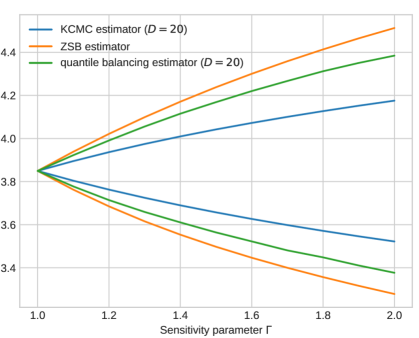
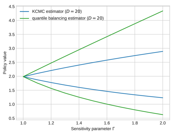
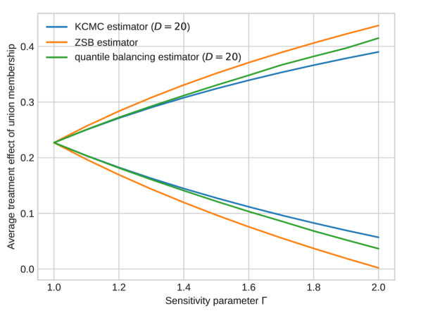
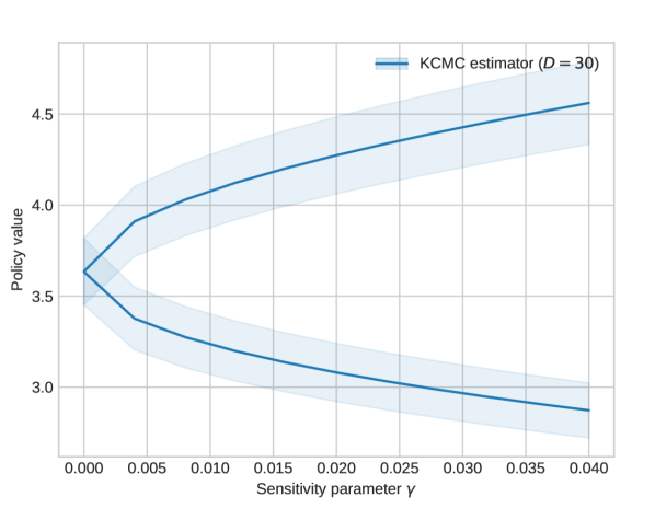
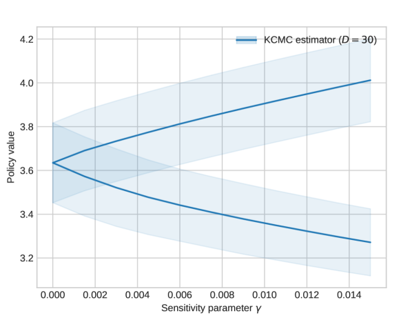
Figure 2 shows the upper and lower bounds of the policy value estimate for binary synthetic data for KCMC estimator (50), ZSB estimator (37), and the quantile balancing (QB) estimator Dorn and Guo (2022) under different confounding levels $\Gamma$. Here, fractional programming is not used in the ZSB estimator and the quantile balancing estimator in order to match the policy value with the KCMC estimator under no confounding (i.e., $\Gamma=1.0$). The feature vectors for the QB estimator and the KCMC estimator were chosen so that they represent the Example 2, where the first stage of the QB estimator solves the modified version of the dual problem for the KCMC estimator. As discussed in Example 2, the QB estimator is always no tighter than the KCMC estimator under such a choice of the feature vector, and it can clearly be observed in this example. Indeed, we can see that the tightness of the bounds loosens as sensitivity parameter $\Gamma$ gets larger. When compared to the sharp estimators (KCMC and QB), the ZSB estimator has looser bounds.

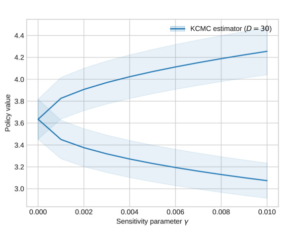
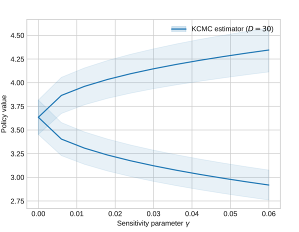
We also present the bounds of the policy values for the synthetic data with continuous action space and real-world data in Figure 3. Please note that in the case of synthetic data with continuous action space, the ZSB estimator cannot be calculated as it requires that the action space be discrete and finite. In both cases, the tightness of the bounds depends on the sensitivity parameter and the type of estimators in the same way as the case of the binary synthetic data.

5.3 Confidence interval

Figure 4: Estimated upper and lower bounds of policy value with 95% confidence interval with (right) and without (left) second-order correction. Solid lines and the bands surrounding them indicate the point estimate (both without second order correction) and its confidence interval.

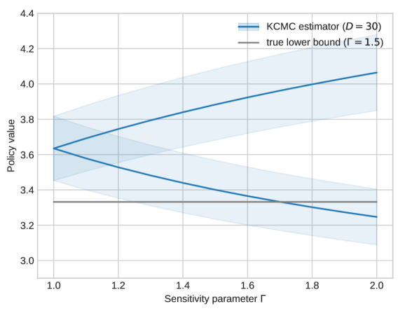
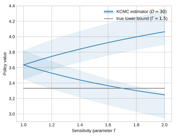
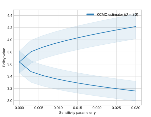
Figure 4 shows the confidence intervals of upper and lower bounds of policy values discussed in Example 5 and 7. Since the second order debiasing term corrects the overly optimistic bounds due to the overfitting, the confidence intervals with the second order correction provide more pessimistic bounds.

Figure 5: Acceptance rate of the null hypothesis under different null hypothesises with Tan’s box constraints ($\Gamma=1.5$) with significance level $\alpha=0.05$. The plot on the left is in the original size and the one on the right is its zoomed version.

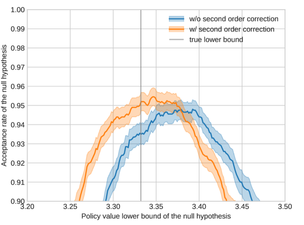
In Figure 5, we show the acceptance rate of the null hypotheses with different values of true lower bound. The acceptance rate is calculated as the coverage rate of the confidence intervals for the synthetic data of sample size 2000, simulated 2000 times. As noted earlier, this synthetic data has an analytically tractable true lower bound and it is indicated by the grey vertical line. As can be expected, acceptance rates of both confidence intervals (with and without second order bias correction) reach their peaks near the true lower bound. However, the confidence interval without second order bias correction has its peaks shifted towards the optimistic direction due to the overfitting in the dual problem and exhibits some level of overrejection at the true null hypothesis compared to its counterpart with the bias correction.

5.4 Model Selection

Figure 6: Estimated policy value lower bound for box constraints ($\Gamma=1.5$), its generalized information criterion, and its 10-fold cross validation (CV) for the synthetic data ($n=1000$) with binary action space.

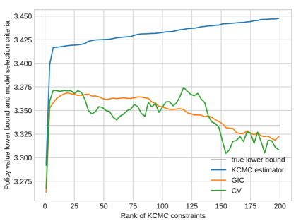
Here, we show an example of using the GIC discussed in Example 6 for rank selection of the KCMC. As the KCMC is a finite dimensional approximation of the infinite dimensional constraints, we have the motivation to increase the rank of the KCMC estimator. On the other hand, the original KCMC lower bound increases monotonously as we increase the rank of KCMC constraints. We can even recover the IPW estimator by making the KCMC full-rank, but this nullifies the confounding robustness, so we would like to avoid using the excessively high rank. This necessitates systematic procedures for selecting the appropriate rank of the KCMC. Fortunately, our dual problem can be interpreted as a standard empirical risk minimization, where the rank selection can be interpreted as the model selection where the cross-validation and the GIC can be used as the selection criteria.

In Figure 6, we plotted the KCMC lower bound estimator, its GIC, and its cross validation. While the original estimator increases monotonically as the rank of the KCMC increases, the GIC and the cross validation start to decline when the rank of the constraints becomes excessively high. In this example, both the GIC and the cross validation seem to prefer ranks around 20, though the cross validation tends to be more noisy and also prefers ranks of around 120.

5.5 f-sensitivity model

(a) KL sensitivity model

(b) Reverse KL sensitivity model

(c) Squared Hellinger sensitivity model

(d) Pearson $\chi^{2}$ sensitivity model

(e) Neyman $\chi^{2}$ sensitivity model

(f) Total variation sensitivity model

Figure 7: Estimated upper and lower bounds of policy value and their confidence intervals using f-sensitivity models. The synthetic data of sample size 4000 with binary action space is used.

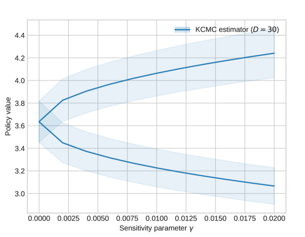
In Figure 7, we present the upper/lower bounds and confidence intervals of the policy value given by the KCMC estimators of f-sensitivity models. Similarly to the example of box constraints, we can see that the f-sensitivity models can produce a continuous control of the level of confounding by the sensitivity parameter. We can also confirm that the confidence intervals behave quite similarly to the case of box constraints.

5.6 Policy learning

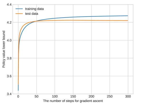
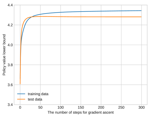
Finally, we consider the max-min policy learning with the KCMC estimator. In the policy learning, we use the gradient ascent on the lower bound estimator similarly to Kallus and Zhou (2018, 2021). As a baseline, we also implemented policy learning with the ZSB estimator using the same dataset and initial policy. In Figure 8, we present the learning curves of both estimators. As can be expected, after the max-min policy learning, the KCMC estimator achieves a higher lower bound than the ZSB estimator, both on the training data and the test data.

Figure 8: Learning curves of the max-min policy learning of logistic policy by the ZSB estimator (left) and the KCMC estimator (right). Both training and test data are binary synthetic data of sample size $1000$. The training curve and the test curve represent the values of each estimator for the data.

6 Conclusion

In this paper, we proposed kernel approximations of the conditional moment constraints that are necessary for sharp sensitivity analysis. Together with the newly introduced conditional f-constraints, our novel formulation with the kernel conditional moment constraints covers a general class of sensitivity analysis models and allows a wider range of applications than previously possible. In the theoretical analysis, we leveraged the convexity to reformulate our estimation method as an empirical risk minimization problem, and established guarantees for consistent policy evaluation and learning by adopting standard proof techniques of the M-estimation. The effectiveness of the kernel conditional moment constraints for sharp sensitivity analysis was demonstrated by our numerical experiments including novel extensions of the sensitivity analysis.

Appendix

Appendix A Notations

notation	meaning
$Y\in\mathcal{Y}$	reward (outcome)
$T\in\mathcal{T}$	action (treatment)
$X\in\mathcal{X}$	context
$U\in\mathcal{U}$	unobserved confounder
$\pi_{\mathrm{base}}(t|x,u)$	unknown (and confounded) base policy from which the data is generated
$\pi(t|x)$	target policy for policy evaluation (or learning)
$p_{\mathrm{obs}}(y,t,x)$	marginal distribution of $(Y,T,X)$ under data generating process (14)
$\mathbb{E},\mathbb{E}_{\mathrm{obs}}$	expectation under data generating process (14)
$\hat{\mathbb{E}}_{n}$	empirical average over $n$ samples generated from (14)
$\mathcal{E}$	uncertainty set of $\pi_{\mathrm{base}}(t|x,u)$
$f_{t,x}(v)$	a convex function w.r.t. $v$ for fixed $t,x$ satisfying $f_{t,x}(1)=1$
$f^{*}_{t,x}(u)$	convex conjugate of $f_{t,x}(v)$
$w(y,t,x)$	reparametrization $w(y,t,x)=\mathbb{E}_{T\sim\pi_{\mathrm{base}}(\cdot|X,U)}\left[\frac{1}{\pi_{\mathrm{base}}(T|X,U)}|Y=y,T=t,X=x\right]$
$\tilde{w}(y,t,x)$	reparametrization $\tilde{w}(y,t,x)=p_{\mathrm{obs}}(t|x)w(y,t,x)$
$\mathcal{W}$	uncertainty set of $w(y,t,x)$, such as $\mathcal{W}^{\mathrm{KCMC}}_{f_{t,x}}$
$\hat{\mathcal{W}}$	uncertainty set of $w(y,t,x)$ defined using empirical samples, such as $\hat{\mathcal{W}}^{\mathrm{KCMC}}_{f_{t,x}}$
$V(\pi)$	value of policy $\pi(t|x)$ under confounded data generating process (18)
$V_{\mathrm{inf}}(\pi)$	lower bound of the policy value of $\pi(t|x)$ under unconfounded model (8)
$\hat{V}_{\mathrm{inf}}(\pi)$	estimator of $V_{\mathrm{inf}}(\pi)$ using empirical samples
$\psi_{d}(t,x)$	$d$-th orthogonal function of kernel conditional moment constraints
$\varphi^{\mathrm{KPCA}}_{d}(t,x)$	$d$-th principal component of kernel PCA fitted to empirical data
$\varphi^{*}_{d}(t,x)$	$d$-th principal component of kernel PCA fitted to population (i.e. infinite data)
$\lambda^{*}_{d}$	the eigenvalue of $\varphi^{*}_{d}(t,x)$
$n$	the number of samples
$D$	the number of kernel conditional moment constraints
$e(y,t,x)$	reparametrization $e(y,t,x):=p_{\mathrm{obs}}(t|x)w(y,t,x)-1$
$r(y,t,x)$	reparametrization $r(y,t,x)=\left(\frac{\pi(t|x)}{p_{\mathrm{obs}}(t|x)}\right)\cdot y$
$\ell_{\theta}(z)$	loss function of dual problems (80) and (86).
$\partial_{\theta}\ell_{\theta}(z)$	subgradient of the loss function w.r.t. $\theta$
$Z$	shorthand notation for observable variables $(Y,T,X)$
$\theta\in\Theta$	parameters of dual loss $(\eta_{f},\eta_{\mathrm{KCMC}})$ or $(\eta_{f},\eta_{\mathrm{KCMC}},\beta)$
$\theta^{*}$	minimizer of population risk $\mathbb{E}\ell_{\theta}(Z)$
$\hat{\theta}_{n}$	minimizer of empirical risk $\hat{\mathbb{E}}_{n}\ell_{\theta}(Z)$
$\Theta_{\varepsilon}$	$\varepsilon$-neighborhood of $(\eta^{*}(\beta),\beta)$ of the partially optimal parameters in policy learning

Table 1: List of common notations used throughout the paper.

Appendix B Omitted Proofs

B.1 Proof of Lemma 4

Proof  Due to the universal property of the kernel, we can approximate $\eta^{*}_{\mathrm{KCMC}}$ with the element of $\mathcal{H}$ arbitrarily well. Therefore, for any $\varepsilon>0$, we can take $D$ such that $\|\Pi_{\boldsymbol{\varphi}^{*}}\eta^{*}_{\mathrm{CMC}}-\eta^{*}_{\mathrm{CMC}}\|\leq\frac{\varepsilon}{3}$ for $\boldsymbol{\varphi}^{*}:=\left(\varphi_{1}^{*},\ldots,\varphi^{*}_{D}\right)^{T}$ and $D\left(\max_{1\leq d\leq D}\frac{c_{d}^{2}}{\lambda^{*}_{d}}\right)\left(\sum_{d=D+1}^{\infty}\lambda_{d}^{*}\right)\leq\frac{\varepsilon}{3}$. For such a choice of $D$, we can prove the statement of the theorem by showing $\operatorname*{plim}_{n\to\infty}\|\Pi_{\boldsymbol{\varphi}^{\mathrm{KPCA}}}\Pi_{\boldsymbol{\varphi}^{*}}\eta^{*}_{\mathrm{CMC}}-\Pi_{\boldsymbol{\varphi}^{*}}\eta^{*}_{\mathrm{CMC}}\|\leq\frac{\varepsilon}{3}$. This is because

$$\|\Pi_{\boldsymbol{\psi}}\eta^{*}_{\mathrm{CMC}}-\eta^{*}_{\mathrm{CMC}}\|$$ (121)

$$=\|\Pi_{\boldsymbol{\varphi}^{\mathrm{KPCA}}}\eta^{*}_{\mathrm{CMC}}-\eta^{*}_{\mathrm{CMC}}\|$$ (122)

$$\leq|\Pi_{\boldsymbol{\varphi}^{\mathrm{KCMC}}}(\eta^{*}_{\mathrm{CMC}}-\Pi_{\boldsymbol{\varphi}^{*}}\eta^{*}_{\mathrm{CMC}})\|+\|\Pi_{\boldsymbol{\varphi}^{\mathrm{KPCA}}}\Pi_{\boldsymbol{\varphi}^{*}}\eta^{*}_{\mathrm{CMC}}-\eta^{*}_{\mathrm{CMC}}\|$$ (123)

$$\leq\|\Pi_{\boldsymbol{\varphi}^{*}}\eta^{*}_{\mathrm{CMC}}-\eta^{*}_{\mathrm{CMC}}\|+\|\Pi_{\boldsymbol{\varphi}^{\mathrm{KPCA}}}\Pi_{\boldsymbol{\varphi}^{*}}\eta^{*}_{\mathrm{CMC}}-\eta^{*}_{\mathrm{CMC}}\|$$ (124)

$$\leq\|\Pi_{\boldsymbol{\varphi}^{*}}\eta^{*}_{\mathrm{CMC}}-\eta^{*}_{\mathrm{CMC}}\|+\|\Pi_{\boldsymbol{\varphi}^{\mathrm{KPCA}}}\Pi_{\boldsymbol{\varphi}^{*}}\eta^{*}_{\mathrm{CMC}}-\Pi_{\boldsymbol{\varphi}^{*}}\eta^{*}_{\mathrm{CMC}}\|+\|\Pi_{\boldsymbol{\varphi}^{*}}\eta^{*}_{\mathrm{CMC}}-\eta^{*}_{\mathrm{CMC}}\|$$ (125)

$$=\|\Pi_{\boldsymbol{\varphi}^{\mathrm{KPCA}}}\Pi_{\boldsymbol{\varphi}^{*}}\eta^{*}_{\mathrm{CMC}}-\Pi_{\boldsymbol{\varphi}^{*}}\eta^{*}_{\mathrm{CMC}}\|+2\|\Pi_{\boldsymbol{\varphi}^{*}}\eta^{*}_{\mathrm{CMC}}-\eta^{*}_{\mathrm{CMC}}\|,$$ (126)

where we used the non-expansive property of the projection operator in the second line.

Now, as we know $\Pi_{\boldsymbol{\varphi}^{*}}\eta^{*}_{\mathrm{CMC}}=\sum_{d=1}^{D}c_{d}\varphi^{*}_{d}$, we have

$$\|\Pi_{\boldsymbol{\varphi}^{\mathrm{KPCA}}}\Pi_{\boldsymbol{\varphi}^{*}}\eta^{*}_{\mathrm{CMC}}-\Pi_{\boldsymbol{\varphi}^{*}}\eta^{*}_{\mathrm{CMC}}\|^{2} =\left\|\Pi_{\boldsymbol{\varphi}^{\mathrm{KPCA}}}\sum_{d=1}^{D}c_{d}\varphi^{*}_{d}-\sum_{d=1}^{D}c_{d}\varphi^{*}_{d}\right\|^{2}$$ (127)

$$=\left\|\sum_{d=1}^{D}\frac{c_{d}}{\sqrt{\lambda^{*}_{d}}}\cdot\sqrt{\lambda^{*}_{d}}(\Pi_{\boldsymbol{\varphi}^{\mathrm{KPCA}}}-1)\varphi^{*}_{d}\right\|^{2}$$ (128)

$$\leq\max_{1\leq d\leq D}\left(\frac{c_{d}^{2}}{\lambda^{*}_{d}}\right)\cdot\left\|\sum_{d=1}^{D}\sqrt{\lambda^{*}_{d}}(\Pi_{\boldsymbol{\varphi}^{\mathrm{KPCA}}}-1)\varphi^{*}_{d}\right\|^{2}$$ (129)

$$\leq\max_{1\leq d\leq D}\left(\frac{c_{d}^{2}}{\lambda^{*}_{d}}\right)\cdot D\sum_{d=1}^{D}\lambda^{*}_{d}\left\|(\Pi_{\boldsymbol{\varphi}^{\mathrm{KPCA}}}-1)\varphi^{*}_{d}\right\|^{2}$$ (130)

$$\leq\max_{1\leq d\leq D}\left(\frac{c_{d}^{2}}{\lambda^{*}_{d}}\right)\cdot D\sum_{d=1}^{\infty}\lambda^{*}_{d}\left\|(\Pi_{\boldsymbol{\varphi}^{\mathrm{KPCA}}}-1)\varphi^{*}_{d}\right\|^{2}$$ (131)

$$=D\cdot\max_{1\leq d\leq D}\left(\frac{c_{d}^{2}}{\lambda^{*}_{d}}\right)\cdot\sum_{d=1}^{\infty}\lambda^{*}_{d}\left(1-\|\Pi_{\boldsymbol{\varphi}^{\mathrm{KPCA}}}\varphi^{*}_{d}\|^{2}\right).$$ (132)

To show that the summation in the last line converges to zero as $n\to\infty$, we use the convergence result of the subspace learned by the kernel PCA in Blanchard et al. (2007, Theorem 3.1.). Their result states that under conditions $\|\Phi(T,X)\|_{\mathcal{H}}^{2}<M_{1}$ and $\|\Phi(T,X)\otimes\bar{\Phi}(T,X)\|<M_{2}$ almost surely, we have

$$0\leq\mathbb{E}\left\|\Pi_{\boldsymbol{\varphi}^{*}}\Phi(T,X)\right\|^{2}-\mathbb{E}\left\|\Pi_{\boldsymbol{\varphi}^{\mathrm{KPCA}}}\Phi(T,X)\right\|^{2}{\overset{p.}{\to}}0$$

as $n\to\infty$, where ${\overset{p.}{\to}}$ indicate the convergence in probability.

Indeed, we can re-write this condition as

$$\mathbb{E} \left\|\Pi_{\boldsymbol{\varphi}^{*}}\Phi(T,X)\right\|^{2}-\mathbb{E}\left\|\Pi_{\boldsymbol{\varphi}^{\mathrm{KPCA}}}\Phi(T,X)\right\|^{2}$$ (133)

$$=\mathbb{E}\left\|\Pi_{\boldsymbol{\varphi}^{*}}\sum_{d=1}^{\infty}\sqrt{\lambda^{*}_{d}}\varphi_{d}^{*}(T,X)\varphi_{d}^{*}\right\|^{2}-\mathbb{E}\left\|\Pi_{\boldsymbol{\varphi}^{\mathrm{KPCA}}}\sum_{d=1}^{\infty}\sqrt{\lambda^{*}_{d}}\varphi_{d}^{*}(T,X)\varphi_{d}^{*}\right\|^{2}$$ (134)

$$=\mathbb{E}\left\|\sum_{d=1}^{\infty}\sqrt{\lambda^{*}_{d}}\varphi_{d}^{*}(T,X)\Pi_{\boldsymbol{\varphi}^{*}}\varphi_{d}^{*}\right\|^{2}-\mathbb{E}\left\|\sum_{d=1}^{\infty}\sqrt{\lambda^{*}_{d}}\varphi_{d}^{*}(T,X)\Pi_{\boldsymbol{\varphi}^{\mathrm{KPCA}}}\varphi_{d}^{*}\right\|^{2}$$ (135)

$$=\mathbb{E}\left\|\sum_{d=1}^{D}\sqrt{\lambda^{*}_{d}}\varphi_{d}^{*}(T,X)\varphi_{d}^{*}\right\|^{2}-\mathbb{E}\left\|\sum_{d=1}^{\infty}\sqrt{\lambda^{*}_{d}}\varphi_{d}^{*}(T,X)\Pi_{\boldsymbol{\varphi}^{\mathrm{KPCA}}}\varphi_{d}^{*}\right\|^{2}$$ (136)

$$=\sum_{d=1}^{D}\lambda^{*}_{d}\mathbb{E}|\varphi_{d}^{*}(T,X)|^{2}\|\varphi_{d}^{*}\|^{2}-\sum_{d=1}^{\infty}\sum_{k=1}^{\infty}\sqrt{\lambda^{*}_{d}}\sqrt{\lambda^{*}_{k}}\left\langle\Pi_{\boldsymbol{\varphi}^{\mathrm{KPCA}}}\varphi_{d}^{*},\Pi_{\boldsymbol{\varphi}^{\mathrm{KPCA}}}\varphi_{k}^{*}\right\rangle_{\mathcal{H}}\mathbb{E}[\varphi_{d}^{*}(T,X),\varphi_{d}^{*}(T,X)]$$ (137)

$$=\sum_{d=1}^{D}\lambda^{*}_{d}\|\varphi_{d}^{*}\|^{2}\cdot\|\varphi_{d}^{*}\|^{2}-\sum_{d=1}^{\infty}\sum_{k=1}^{\infty}\sqrt{\lambda^{*}_{d}}\sqrt{\lambda^{*}_{k}}\left\langle\Pi_{\boldsymbol{\varphi}^{\mathrm{KPCA}}}\varphi_{d}^{*},\Pi_{\boldsymbol{\varphi}^{\mathrm{KPCA}}}\varphi_{k}^{*}\right\rangle_{\mathcal{H}}\left\langle\varphi_{d}^{*},\varphi_{k}^{*}\right\rangle_{\mathcal{H}}$$ (138)

$$=\sum_{d=1}^{D}\lambda^{*}_{d}-\sum_{d=1}^{\infty}\sum_{k=1}^{\infty}\sqrt{\lambda^{*}_{d}}\sqrt{\lambda^{*}_{k}}\left\langle\Pi_{\boldsymbol{\varphi}^{\mathrm{KPCA}}}\varphi_{d}^{*},\Pi_{\boldsymbol{\varphi}^{\mathrm{KPCA}}}\varphi_{k}^{*}\right\rangle_{\mathcal{H}}\mathbbm{1}_{d=k}$$ (139)

$$=\sum_{d=1}^{D}\lambda^{*}_{d}-\sum_{d=1}^{\infty}\lambda^{*}_{d}\left\|\Pi_{\boldsymbol{\varphi}^{\mathrm{KPCA}}}\varphi_{d}^{*}\right\|^{2}$$ (140)

$$=\sum_{d=1}^{\infty}\lambda^{*}_{d}-\sum_{d=D+1}^{\infty}\lambda^{*}_{d}-\sum_{d=1}^{\infty}\lambda^{*}_{d}\left\|\Pi_{\boldsymbol{\varphi}^{\mathrm{KPCA}}}\varphi_{d}^{*}\right\|^{2}$$ (141)

$$=\sum_{d=1}^{\infty}\lambda^{*}_{d}\left(1-\|\Pi_{\boldsymbol{\varphi}^{\mathrm{KPCA}}}\varphi_{d}^{*}\|^{2}\right)-\sum_{d=D+1}^{\infty}\lambda^{*}_{d}$$ (142)

$${\overset{p.}{\to}}0.$$ (143)

Therefore, we have

$$\operatorname*{plim}_{n\to\infty}\| \Pi_{\boldsymbol{\varphi}^{\mathrm{KPCA}}}\Pi_{\boldsymbol{\varphi}^{*}}\eta^{*}_{\mathrm{CMC}}-\Pi_{\boldsymbol{\varphi}^{*}}\eta^{*}_{\mathrm{CMC}}\|^{2}$$ (144)

$$\leq\operatorname*{plim}_{n\to\infty}D\cdot\max_{1\leq d\leq D}\left(\frac{c_{d}^{2}}{\lambda^{*}_{d}}\right)\cdot\left(\mathbb{E}\left\|\Pi_{\boldsymbol{\varphi}^{*}}\Phi(T,X)\right\|^{2}-\mathbb{E}\left\|\Pi_{\boldsymbol{\varphi}^{\mathrm{KPCA}}}\Phi(T,X)\right\|^{2}+\sum_{d=D+1}^{\infty}\lambda^{*}_{d}\right)$$ (145)

$$\leq D\cdot\max_{1\leq d\leq D}\left(\frac{c_{d}^{2}}{\lambda^{*}_{d}}\right)\cdot\operatorname*{plim}_{n\to\infty}\left(\mathbb{E}\left\|\Pi_{\boldsymbol{\varphi}^{*}}\Phi(T,X)\right\|^{2}-\mathbb{E}\left\|\Pi_{\boldsymbol{\varphi}^{\mathrm{KPCA}}}\Phi(T,X)\right\|^{2}\right)+\frac{\varepsilon}{3}$$ (146)

$$=\frac{\varepsilon}{3},$$ (147)

which concludes the proof.  

In the above proof, the most obscure assumption for readers would be the condition that $\lim_{D\to\infty}\left\{D\left(\max_{1\leq d\leq D}\frac{c_{d}^{2}}{\lambda_{d}^{*}}\right)\left(\sum_{d=D+1}^{\infty}\lambda_{d}^{*}\right)\right\}=0$. This assumption can be approximately decomposed into two slightly more interpretable assumptions. First, it requires that $\max_{1\leq d\leq D}\frac{c_{d}^{2}}{\lambda_{d}^{*}}$ is bounded so that basis function $\varphi^{*}_{d}$ for smaller spectrum $\lambda^{*}_{d}$ constitutes proportionally smaller part of function $\eta^{*}_{\mathrm{CMC}}$. For example, if $\eta_{\mathrm{CMC}}^{*}$ happens to coincide with a function generated from the Gaussian process with kernel $k(\cdot,\cdot)$, it will satisfy this property with high probability. Second, it requires that $\sum_{d=D+1}^{\infty}\lambda_{d}^{*}=o_{p}(\frac{1}{D})$ so that the decay of spectrum $\lambda^{*}_{d}$ is fast. In fact, this assumption is similar to another assumption $\|\Phi(T,X)\|^{2}_{\mathcal{H}}\leq M_{1}$ we made, because this assumption leads to $M_{1}\geq\mathbb{E}\|\Phi(T,X)\|_{\mathcal{H}}^{2}=\mathbb{E}\left\|\sum_{d=1}^{\infty}\sqrt{\lambda_{d}^{*}}\varphi_{d}(T,X)\varphi_{d}\right\|^{2}=\sum_{d=1}^{\infty}\lambda_{d}^{*}\mathbb{E}|\varphi_{d}(T,X)|^{2}\cdot\|\varphi_{d}\|^{2}=\sum_{d=1}^{\infty}\lambda_{d}^{*}$, which implies convergence of its tail part $\sum_{d=D+1}^{\infty}\lambda_{d}^{*}\to 0$.

B.2 Proof of Theorem 9

Proof  Due to the concavity of policy class $\{\pi_{\beta}(t|x):\ \beta\in\mathcal{B}\}$, we know that $\beta\mapsto\mathbb{E}\left[\tilde{w}(Y,T,X)\left(\frac{\pi_{\beta}(T|X)}{p_{\mathrm{obs}}(T|X)}\right)Y\right]$ is concave for any $t\in\mathcal{T}$ and $x\in\mathcal{X}$. Then, we can see that

$$\max_{\beta\in\mathcal{B}}V_{\mathrm{inf}}^{\mathrm{KCMC}} =\max_{\beta\in\mathcal{B}}\max_{\begin{subarray}{c}\eta_{\mathrm{KCMC}}\in\mathbb{R}^{D}\\ \eta_{f}>0\end{subarray}}\min_{\tilde{w}}\mathbb{E}\left[\tilde{w}(Y,T,X)\left(\frac{\pi_{\beta}(T|X)}{p_{\mathrm{obs}}(T|X}\right)Y\right]$$ (148)

$$\quad\quad\quad\quad\quad\quad\quad\quad\quad\quad-\mathbb{E}\left[(\tilde{w}-1){\eta_{\mathrm{KCMC}}}^{T}\boldsymbol{\psi}\right]+\eta_{f}\left(\mathbb{E}[f_{T,X}(\tilde{w})]-\gamma\right)$$ (149)

$$=\max_{\beta\in\mathcal{B}}\max_{\begin{subarray}{c}\eta_{\mathrm{KCMC}}\in\mathbb{R}^{D}\\ \eta_{f}>0\end{subarray}}\mathbb{E}[-\ell_{\theta}(Y,T,X)]$$ (150)

$$=\max_{\theta\in\Theta}\mathbb{E}[-\ell_{\theta}(Y,T,X)]$$ (151)

is a concave maximization problem, because $\mathbb{E}[\ell_{\theta}]$ is the pointwise infimum of concave functions. Thus, we can apply Lemma 7 and get $\hat{\theta}_{n}{\overset{p.}{\to}}\theta^{*}$, which implies $\hat{\theta}_{n}$ tend to the inside of compact set $\{\theta\in\Theta:\ \|\theta-\theta^{*}\|\leq\varepsilon\}$, where we have uniform convergence guarantee of $\hat{\mathbb{E}}_{n}[\ell_{\theta}(Z)]$ due to Lemma 6. Therefore, we have

$$0 \leq\hat{V}_{\mathrm{inf}}^{\mathrm{KCMC}}(\pi_{\hat{\beta}})-\hat{V}_{\mathrm{inf}}^{\mathrm{KCMC}}(\pi_{\beta^{*}})$$

$$=-\hat{\mathbb{E}}_{n}[\ell_{\hat{\theta}_{n}}(Z)]+\hat{\mathbb{E}}_{n}[\ell_{\theta^{*}}(Z)]$$

$$=\left[-\hat{\mathbb{E}}_{n}[\ell_{\hat{\theta}_{n}}(Z)]+\mathbb{E}[\ell_{\hat{\theta}_{n}}(Z)]\right]+\left[\hat{\mathbb{E}}_{n}[\ell_{\theta^{*}}(Z)]-\mathbb{E}[\ell_{\theta^{*}}(Z)]\right]-\left[\mathbb{E}[\ell_{\hat{\theta}_{n}}(Z)]-\mathbb{E}[\ell_{\theta^{*}}(Z)]\right]$$

$$\leq\left[-\hat{\mathbb{E}}_{n}[\ell_{\hat{\theta}_{n}}(Z)]+\mathbb{E}[\ell_{\hat{\theta}_{n}}(Z)]\right]+\left[\hat{\mathbb{E}}_{n}[\ell_{\theta^{*}}(Z)]-\mathbb{E}[\ell_{\theta^{*}}(Z)]\right]$$

$${\overset{p.}{\to}}\ 0,$$

which implies $\hat{V}_{\mathrm{inf}}^{\mathrm{KCMC}}(\pi_{\hat{\beta}}){\overset{p.}{\to}}\hat{V}_{\mathrm{inf}}^{\mathrm{KCMC}}(\pi_{\beta^{*}})$. Lastly, due to the law of large numbers, we have $\hat{V}_{\mathrm{inf}}^{\mathrm{KCMC}}(\pi_{\beta^{*}}){\overset{p.}{\to}}V_{\mathrm{inf}}^{\mathrm{KCMC}}(\pi_{\beta^{*}})$, which concludes the proof.  

B.3 Proof of Theorem 11

Let us define $\Theta_{\varepsilon}:=\left\{\left(\eta,\beta\right):\|\eta-\eta^{*}(\beta)\|\leq\varepsilon,\beta\in\mathcal{B}\right\}$ for $\eta^{*}(\beta):=\arg\min_{\eta\in H}\mathbb{E}[\ell_{\beta,\eta}(Z)]$, which is the $\varepsilon$-neighborhood of the partially optimized parameters. We begin by showing uniform convergence $\sup_{\theta\in\Theta_{\varepsilon}}\left|\hat{\mathbb{E}}_{n}\ell_{\theta}(Z)-\mathbb{E}\ell_{\theta}(Z)\right|{\overset{p.}{\to}}0$ for some $\varepsilon>0$. For the proof of Theorem 11, we need the following lemmas:

Lemma 14 (Stability of VC functions (Vaart and Wellner, 1996, Lemma 2.6.18)).

Let $\mathcal{F},\mathcal{G}$ be VC classes of functions on $\mathcal{Z}$ and $\mathbb{R}^{D}$. Let $h_{1}:\mathcal{Z}\to\mathbb{R}$, $h_{2}:\mathcal{Z}\to\mathbb{R}^{D}$ be fixed functions. Then, product functions $h_{1}\cdot\mathcal{F}:=\{h_{1}\cdot f:f\in\mathcal{F}\}$ and composite functions $\mathcal{G}\circ h_{2}:=\{g\circ h_{2}:g\in\mathcal{G}\}$ are VC.

Definition 15 (Covering number (Van de Geer, 2020, Definition 6.1.2.)).

A class of functions $\mathcal{G}^{(\delta)}$ is said to be a $\delta$-covering of $\mathcal{G}$ on $\mathcal{Z}$ with respect to $L_{1}(\mathcal{Z},\mathbb{E})$ norm if

$$\sup_{g\in\mathcal{G}}\inf_{\tilde{g}\in\mathcal{G}^{(\delta)}}\mathbb{E}\left|g(Z)-\tilde{g}(Z)\right|\leq\delta.$$ (152)

Additionally, the covering number of $\mathcal{G}$ is defined as the minimal cardinality of its $\delta$-covering so that

$$N_{1}(\delta,\mathcal{G},\mathbb{E})=\min\left\{\left|\mathcal{G}^{(\delta)}\right|:\ \mathcal{G}^{(\delta)}\text{ is a $\delta$-covering of $\mathcal{G}$ w.r.t. }L_{1}(\mathcal{Z},\mathbb{E})\text{ norm}\right\}.$$ (153)

Lemma 16 (Covering number of a VC class (Van de Geer, 2020, Theorem 6.4.1)).

Let $Q$ be any probability measure on $\mathcal{Z}$ and let $N_{1}(\cdot,\mathcal{G},\mathbb{E}_{Q})$ be the covering number of $\mathcal{G}$. For a VC class $\mathcal{G}$ with VC dimension $V$ and bounded envelope $G(z):=\sup_{g\in\mathcal{G}}|g(z)|$ such that $\mathbb{E}_{Q}[G(Z)]<\infty$, we have a constant $A$ depending only on $V$ (not on $Q$) satisfying $N_{1}(\delta\mathbb{E}_{Q}[G],\mathcal{G},\mathbb{E}_{Q})\leq\max(A\delta^{-2V},\exp{\delta/4})$ for any $\delta>0$.

Lemma 17 (Uniform convergence (Van de Geer, 2020, Theorem 6.1.2)).

Suppose $\mathbb{E}[G(Z)]<\infty$ for $G(z):=\sup_{g\in\mathcal{G}}g(z)$ and $\frac{\log N_{1}(\delta,\mathcal{G},\hat{\mathbb{E}}_{n})}{n}{\overset{p.}{\to}}0$ for any $\delta>0$. Then, $\sup_{g\in\mathcal{G}}|\hat{\mathbb{E}}_{n}g-\mathbb{E}g|{\overset{p.}{\to}}0$.

Lemma 18 ($L_{1}(\mathcal{Z},\mathbb{E})$ envelope of $\eta\mapsto\partial_{\eta}\ell_{\eta,\beta}(z)$).

Under Condition 10, there exist $\varepsilon>0$ such that envelopes $G^{\partial_{\eta_{f}}\ell}_{\varepsilon}(z):=\sup_{\begin{subarray}{c}\delta\ell\in\partial_{\eta_{f}}\ell_{\theta}(z)\\ \theta\in\Theta_{\varepsilon}\end{subarray}}\left|\delta\ell\right|$ and $G^{\partial_{\eta_{\mathrm{KCMC}}}\ell}_{\varepsilon}(z):=\sup_{\begin{subarray}{c}\delta\ell\in\partial_{\eta_{\mathrm{KCMC}}}\ell_{\theta}(z)\\ \theta\in\Theta_{\varepsilon}\end{subarray}}\left\|\delta\ell\right\|$ satisfy $\mathbb{E}G^{\partial_{\eta_{f}}\ell}_{\varepsilon}(Z)<\infty$ and $\mathbb{E}G^{\partial_{\eta_{\mathrm{KCMC}}}\ell}_{\varepsilon}(Z)<\infty$.

Proof  Let us take $\varepsilon>0$ sufficiently small so that envelopes $G^{\boldsymbol{\psi}}(z)$, $G^{f^{*}}_{\varepsilon}(z)$, and $R(z)$ are in $L_{1}(\mathcal{Z},\mathbb{E})$. We can show that $\left\{z\mapsto\partial_{\eta_{f}}\ell_{\theta}(z):\theta\in\Theta_{\varepsilon}\right\}$ has $L_{1}(\mathcal{Z},\mathbb{E})$ envelope $G^{\partial_{\eta_{f}}\ell}_{\varepsilon}(z):=\sup_{\begin{subarray}{c}\delta_{\eta_{f}}\ell\in\partial_{\eta_{f}}\ell_{\theta}(z)\\ \theta\in\Theta_{\varepsilon}\end{subarray}}\left|\delta_{\eta_{f}}\ell\right|\leq\gamma+G^{f^{*}}_{\varepsilon}(z)+L\left(\frac{\bar{\eta}_{\mathrm{KCMC}}G^{\boldsymbol{\psi}}(z)+R(z)}{\underaccent{\bar}{\eta}_{f}-\varepsilon}\right)$ because

$$\partial_{\eta_{f}}\ell_{\theta}(z) =\gamma+f_{t,x}^{*}\left(\frac{{\eta_{\mathrm{KCMC}}}^{T}\boldsymbol{\psi}(t,x)-\left(\frac{\pi_{\beta}(t|x)}{p_{\mathrm{obs}}(t|x)}\right)y}{\eta_{f}}\right)$$ (154)

$$\quad\quad+\left(\frac{{\eta_{\mathrm{KCMC}}}^{T}\boldsymbol{\psi}(t,x)-\left(\frac{\pi_{\beta}(t|x)}{p_{\mathrm{obs}}(t|x)}\right)y}{\eta_{f}}\right)\partial_{\eta_{f}}f_{t,x}^{*}\left(\frac{{\eta_{\mathrm{KCMC}}}^{T}\boldsymbol{\psi}(t,x)-\left(\frac{\pi_{\beta}(t|x)}{p_{\mathrm{obs}}(t|x)}\right)y}{\eta_{f}}\right).$$ (155)

Similarly, we can see $\left\{z\mapsto\partial_{\eta_{\mathrm{KCMC}}}\ell_{\theta}(z):\theta\in\Theta_{\varepsilon}\right\}$ also has $L_{1}(\mathcal{Z},\mathbb{E})$ envelope $G^{\partial_{\eta_{\mathrm{KCMC}}}\ell}_{\varepsilon}(z):=\sup_{\begin{subarray}{c}\delta\ell\in\partial_{\eta_{\mathrm{KCMC}}}\ell_{\theta}(z)\\ \theta\in\Theta_{\varepsilon}\end{subarray}}\left\|\delta\ell\right\|\leq(L+1)G^{\boldsymbol{\psi}}(z)$ as

$$\partial_{\eta_{\mathrm{KCMC}}}\ell_{\theta}(z) =\boldsymbol{\psi}(t,x)\left\{1-\partial f_{t,x}^{*}\left(\frac{{\eta_{\mathrm{KCMC}}}^{T}\boldsymbol{\psi}(t,x)-\left(\frac{\pi_{\beta}(t|x)}{p_{\mathrm{obs}}(t|x)}\right)y}{\eta_{f}}\right)\right\},$$ (156)

which concludes the proof.  

Lemma 19 (Uniform convergence over $\Theta_{\varepsilon}$).

Assume policy class $\{\pi_{\beta}(t|x):\ \beta\in\mathcal{B}\}$ is VC and that Condition 10 is met. Then, there exits $\varepsilon>0$ such that

$$\sup_{\theta\in\Theta_{\varepsilon}}{\left|\hat{\mathbb{E}}_{n}\ell_{\theta}(Z)-\mathbb{E}\ell_{\theta}(Z)\right|}{\overset{p.}{\to}}0.$$

Proof  Remember that loss function $\ell:\Theta\times\mathcal{Z}\to\mathbb{R}$ is defined as

$$\ell_{\theta}(t,y,x):=\eta_{f}\gamma-{\eta_{\mathrm{KCMC}}}^{T}\boldsymbol{\psi}(t,x)+\eta_{f}f_{t,x}^{*}\left(\frac{{\eta_{\mathrm{KCMC}}}^{T}\boldsymbol{\psi}(t,x)-\left(\frac{\pi_{\beta}(t|x)}{p_{\mathrm{obs}}(t|x)}\right)y}{\eta_{f}}\right).$$ (157)

We choose $\varepsilon$ such that envelopes $G^{\boldsymbol{\psi}}(z)$, $G^{f^{*}}_{\varepsilon}(z)$, and $R(z)$ are in $L_{1}(\mathcal{Z},\mathbb{E})$. Then, $\{z\mapsto\ell_{\theta}(z):\theta\in\Theta_{\varepsilon}\}$ has $L_{1}(\mathcal{Z},\mathbb{E})$ envelope $G^{\ell}_{\varepsilon}(z):=\sup_{\theta\in\Theta_{\varepsilon}}\left|\ell_{\theta}(z)\right|\leq\gamma\eta_{f}+\bar{\eta}_{\mathrm{KCMC}}G^{\boldsymbol{\psi}}_{\varepsilon}(z)+\eta_{f}G^{f^{*}}_{\varepsilon}(z)$.

Now, we would like to show that the class of loss functions $\mathcal{G}_{\varepsilon}:=\{\ell_{\theta}:\theta\in\Theta_{\varepsilon}\}$ has $\delta$-covering satisfying $\frac{N_{1}(\delta,\mathcal{G},\hat{\mathbb{E}}_{n})}{n}{\overset{p.}{\to}}0$ for some $\varepsilon>0$. First, we know that

$$\mathcal{G}^{\prime}_{\varepsilon}=\left\{(y,t,x)\mapsto{\eta_{\mathrm{KCMC}}}^{T}\boldsymbol{\psi}(t,x):\left(\eta,\beta\right)\in\Theta_{\varepsilon}\right\}$$

and

$$\mathcal{G}^{\prime\prime}_{\varepsilon}=\left\{(y,t,x)\mapsto\left(\frac{\pi_{\beta}(t|x)}{p_{\mathrm{obs}}(t|x)}\right)y:\beta\in\mathcal{B}\right\}$$

are VC classes by Lemma 14. Thus, by Lemma 16, there exist $\frac{\delta}{3(L+1)}$-covering of these satisfying $\frac{\log N_{1}(\delta/3(L+1),\mathcal{G}^{\prime}_{\varepsilon},\hat{\mathbb{E}}_{n})}{n}{\overset{p.}{\to}}0$ and $\frac{\log N_{1}(\delta/3(L+1),\mathcal{G}^{\prime\prime}_{\varepsilon},\hat{\mathbb{E}}_{n})}{n}{\overset{p.}{\to}}0$. We let $H_{\mathrm{KCMC}}^{(\delta)}=\{\eta_{\mathrm{KCMC},k}^{(\delta)}:k=1,\ldots,N_{1}(\delta/3(L+1),\mathcal{G}^{\prime}_{\varepsilon},\hat{\mathbb{E}}_{n})\}$ and $\mathcal{B}^{(\delta)}=\{\beta_{k}^{(\delta)}:k=1,\ldots,N_{1}(\delta/3(L+1),\mathcal{G}^{\prime\prime}_{\varepsilon},\hat{\mathbb{E}}_{n})\}$ denote the parameter sets corresponding to such coverings. Also, we can take $\frac{\delta}{3M}$-mesh of $\{\eta_{f}:\eta_{f}\in[\underaccent{\bar}{\eta}_{f}-\varepsilon,\bar{\eta}_{f}+\varepsilon]\}$ as $H_{f}^{(\delta)}:=\left\{\frac{\delta k}{3M}:k\in\mathbb{Z}\right\}\cap\left[\underaccent{\bar}{\eta}_{f}-\varepsilon,\bar{\eta}_{f}+\varepsilon\right]$ for $M:=2\mathbb{E}G^{\partial_{\eta_{f}}\ell}_{\varepsilon}(Z)$, where $G^{\partial_{\eta_{f}}\ell}_{\varepsilon}(Z)$ is as defined in Lemma 18. Clearly, the cardinality of $H_{f}^{(\delta)}$ does not depend on the sample size $n$ and $\frac{\log|H^{(\delta)}_{f}|}{n}\to 0$.

Now, we can show that $\Theta^{(\delta)}:=H_{f}^{(\delta)}\times H_{\mathrm{KCMC}}^{(\delta)}\times\mathcal{B}^{(\delta)}$ becomes $\delta$-covering of $\mathcal{G}_{\varepsilon}$. For any $\left(\eta_{f},\eta_{\mathrm{KCMC}},\beta\right)\in\Theta_{\varepsilon}$, we can take $\left(\eta_{f}^{(\delta)},\eta_{\mathrm{KCMC}}^{(\delta)},\beta^{(\delta)}\right)\in H_{f}^{(\delta)}\times H_{\mathrm{KCMC}}^{(\delta)}\times\mathcal{B}^{(\delta)}$ such that

$$|\eta_{f}-\eta_{f}^{(\delta)}|\leq\frac{\delta}{3M},$$ (158)

$$\hat{\mathbb{E}}_{n}\left|{\eta_{\mathrm{KCMC}}}^{T}\boldsymbol{\psi}(T,X)-{\eta_{\mathrm{KCMC}}^{(\delta)}}^{T}\boldsymbol{\psi}(T,X)\right|\leq\frac{\delta}{3(L+1)},$$ (159)

and

$$\hat{\mathbb{E}}_{n}\left|\left(\frac{\pi_{\beta}(T|X)}{p_{\mathrm{obs}}(T|X)}\right)Y-\left(\frac{\pi_{\beta^{(\delta)}}(T|X)}{p_{\mathrm{obs}}(T|X)}\right)Y\right|\leq\frac{\delta}{3(L+1)}.$$ (160)

Thus, we have

$$\hat{\mathbb{E}}_{n}\left|\ell_{\eta_{f},\eta_{\mathrm{KCMC}},\beta}(Z)-\ell_{\eta_{f}^{(\delta)},\eta_{\mathrm{KCMC}},\beta}(Z)\right| \leq\hat{\mathbb{E}}_{n}\sup_{\begin{subarray}{c}\delta_{\eta_{f}}\ell\in\partial_{\eta_{f}}\ell_{\theta}(Z)\\ \theta\in\Theta_{\varepsilon}\end{subarray}}\left|\delta_{\eta_{f}}\ell\right|\left|\eta_{f}-\eta_{f}^{(\delta)}\right|$$ (161)

$$\leq\hat{\mathbb{E}}_{n}G_{\varepsilon}^{\partial_{\eta_{f}}\ell}(Z)\left|\eta_{f}-\eta_{f}^{(\delta)}\right|$$ (162)

$${\overset{p.}{\to}}\frac{M}{2}\cdot\frac{\delta}{3M}$$ (163)

$$<\frac{\delta}{3}.$$ (164)

and

$$\hat{\mathbb{E}}_{n}\left|\ell_{\eta_{f}^{(\delta)},\eta_{\mathrm{KCMC}},\beta}(Z)-\ell_{\eta_{f}^{(\delta)},\eta_{\mathrm{KCMC}}^{(\delta)},\beta^{(\delta)}}(Z)\right|$$ (165)

$$\leq\hat{\mathbb{E}}_{n}\left|J_{\eta_{f}^{(\delta)}}\left({\eta_{\mathrm{KCMC}}}^{T}\boldsymbol{\psi}(T,X),\left(\frac{\pi_{\beta}(T|X)}{p_{\mathrm{obs}}(T|X)}\right)Y,T,X\right)-J_{\eta_{f}^{(\delta)}}\left({\eta_{\mathrm{KCMC}}^{(\delta)}}^{T}\boldsymbol{\psi}(T,X),\left(\frac{\pi_{\beta^{(\delta)}}(T|X)}{p_{\mathrm{obs}}(T|X)}\right)Y,T,X\right)\right|$$ (166)

$$\quad\leq\hat{\mathbb{E}}_{n}\left[\sup_{\begin{subarray}{c}\delta J\in\partial_{(h,r)}J_{\eta_{f}^{(\delta)}}(h,r,t,x),\\ h,r\in\mathbb{R},t\in\mathcal{T},x\in\mathcal{X}\end{subarray}}{\left\|\delta J\right\|_{\infty}}\cdot\left\|\left(\begin{array}[]{c}{\eta_{\mathrm{KCMC}}}^{T}\boldsymbol{\psi}(T,X)-{\eta_{\mathrm{KCMC}}^{(\delta)}}^{T}\boldsymbol{\psi}(T,X)\\ \left(\frac{\pi_{\beta}(T|X)}{p_{\mathrm{obs}}(T|X)}\right)Y-\left(\frac{\pi_{\beta^{(\delta)}}(T|X)}{p_{\mathrm{obs}}(T|X)}\right)Y\end{array}\right)\right\|_{1}\right]$$ (169)

$$\quad\leq\hat{\mathbb{E}}_{n}\left[\left\|\left(\begin{array}[]{c}1+L\\ L\end{array}\right)\right\|_{\infty}\cdot\left\|\left(\begin{array}[]{c}{\eta_{\mathrm{KCMC}}}^{T}\boldsymbol{\psi}(T,X)-{\eta_{\mathrm{KCMC}}^{(\delta)}}^{T}\boldsymbol{\psi}(T,X)\\ \left(\frac{\pi_{\beta}(T|X)}{p_{\mathrm{obs}}(T|X)}\right)Y-\left(\frac{\pi_{\beta^{(\delta)}}(T|X)}{p_{\mathrm{obs}}(T|X)}\right)Y\end{array}\right)\right\|_{1}\right]$$ (174)

$$\quad\leq(L+1)\cdot\left(\hat{\mathbb{E}}_{n}\left|{\eta_{\mathrm{KCMC}}}^{T}\boldsymbol{\psi}(T,X)-{\eta_{\mathrm{KCMC}}^{(\delta)}}^{T}\boldsymbol{\psi}(T,X)\right|+\hat{\mathbb{E}}_{n}\left|\left(\frac{\pi_{\beta}(T|X)}{p_{\mathrm{obs}}(T|X)}\right)Y-\left(\frac{\pi_{\beta^{(\delta)}}(T|X)}{p_{\mathrm{obs}}(T|X)}\right)Y\right|\right)$$ (175)

$$\quad\leq(L+1)\cdot\frac{2\delta}{3(L+1)}=\frac{2\delta}{3},$$ (176)

where $J_{\eta_{f}}(h,r,t,x):=-h+\eta_{f}f^{*}_{t,x}\left(\frac{h-r}{\eta_{f}}\right)$. The subgradients of $J_{\eta_{f}}$ can be calculated as $\partial_{h}J_{\eta_{f}}(h,r,t,x):=-1+\partial f^{*}_{t,x}\left(\frac{h-r}{\eta_{f}}\right)$ and $\partial_{r}J_{\eta_{f}}(h,r,t,x):=-\partial f^{*}_{t,x}\left(\frac{h-r}{\eta_{f}}\right)$ whose absolute value can be bounded by $|1+L|$ and $|L|$ respectively. Finally, by combining (164) and (176), we get

$$\hat{\mathbb{E}}_{n}\left|\ell_{\eta_{f},\eta_{\mathrm{KCMC}},\beta}(Z)-\ell_{\eta_{f}^{(\delta)},\eta_{\mathrm{KCMC}}^{(\delta)},\beta^{(\delta)}}(Z)\right|\leq\delta$$ (177)

with high probability as $n\to\infty$. Thus, $\Theta^{(\delta)}$ is a $\delta$-covering of $\Theta_{\varepsilon}$ satisfying $\frac{\log|\Theta^{(\delta)}|}{n}{\overset{p.}{\to}}0$. Thus, we conclude that

$$\sup_{\theta\in\Theta_{\varepsilon}}{\left|\hat{\mathbb{E}}_{n}\ell_{\theta}(Z)-\mathbb{E}\ell_{\theta}(Z)\right|}{\overset{p.}{\to}}0$$

by Lemma 17.  

Finally, with the lemmas above, we can prove Theorem 11.

Proof  Here, our aim is to prove the uniform convergence of the KCMC estimator over the policy class, i.e.

$$\sup_{\beta\in\mathcal{B}}\left|\hat{V}_{\mathrm{inf}}^{\mathrm{KCMC}}(\pi_{\beta})-V_{\mathrm{inf}}^{\mathrm{KCMC}}(\pi_{\beta})\right|{\overset{p.}{\to}}0.$$ (178)

Let $\hat{\eta}(\beta):=\arg\min_{\eta\in H}\hat{\mathbb{E}}_{n}\left[\ell_{\beta,\eta}(Z)\right]$. Let us also use Lemma 19 to take $\varepsilon>0$ so that

$$\sup_{\theta\in\Theta_{\varepsilon}}{\left|\hat{\mathbb{E}}_{n}\ell_{\theta}(Z)-\mathbb{E}\ell_{\theta}(Z)\right|}{\overset{p.}{\to}}0.$$

For this choice of $\varepsilon$ and any $\beta\in\mathcal{B}$, let us define

$$\tilde{\eta}(\beta):=\frac{\varepsilon}{\varepsilon+\|\hat{\eta}(\beta)-\eta^{*}(\beta)\|}\cdot\hat{\eta}(\beta)+\frac{\|\hat{\eta}(\beta)-\eta^{*}(\beta)\|}{\varepsilon+\|\hat{\eta}(\beta)-\eta^{*}(\beta)\|}\cdot\eta^{*}(\beta)$$ (179)

so that it becomes a linear interpolation between $\hat{\eta}(\beta)$ and $\eta^{*}(\beta)$ that is always included in the $\varepsilon$ neighborhood of $\eta^{*}(\beta)$ so that $\|\tilde{\eta}(\beta)-\eta^{*}(\beta)\|\leq\varepsilon$. Since $\eta\mapsto\ell_{\eta,\beta}(z)$ is convex for any $z\in\mathcal{Z}$ and any $\beta\in\mathcal{B}$, we have

$$\hat{\mathbb{E}}_{n}[\ell_{\tilde{\eta}(\beta),\beta}(Z)]\leq\frac{\varepsilon}{\varepsilon+\|\hat{\eta}(\beta)-\eta^{*}(\beta)\|}\cdot\hat{\mathbb{E}}_{n}[\ell_{\hat{\eta}(\beta),\beta}(Z)]+\frac{\|\hat{\eta}(\beta)-\eta^{*}(\beta)\|}{\varepsilon+\|\hat{\eta}(\beta)-\eta^{*}(\beta)\|}\cdot\hat{\mathbb{E}}_{n}[\ell_{\eta^{*}(\beta),\beta}(Z)].$$ (180)

As the optimality of $\hat{\eta}(\beta)$ with respect to $\beta\mapsto\hat{\mathbb{E}}_{n}\ell_{\eta,\beta}(Z)$ implies $0\leq\hat{\mathbb{E}}_{n}[\ell_{\tilde{\eta}(\beta),\beta}(Z)]-\hat{\mathbb{E}}_{n}[\ell_{\hat{\eta}(\beta),\beta}(Z)]$, we get

$$0\leq\hat{\mathbb{E}}_{n}[\ell_{\eta^{*}(\beta),\beta}(Z)]-\hat{\mathbb{E}}_{n}[\ell_{\tilde{\eta}(\beta),\beta}(Z)].$$ (181)

Since $(\eta^{*}(\beta),\beta)$ and $(\tilde{\eta}(\beta),\beta)$ are included in $\Theta_{\varepsilon}$, we can use Lemma 19 to see

$$0 \leq\sup_{\beta\in\mathcal{B}}\left[\mathbb{E}[\ell_{\tilde{\eta}(\beta),\beta}(Z)]-\mathbb{E}[\ell_{\eta^{*}(\beta),\beta}(Z)]\right]$$ (182)

$$\leq\sup_{\beta\in\mathcal{B}}\Bigl{[}\left(\mathbb{E}[\ell_{\tilde{\eta}(\beta),\beta}(Z)]-\hat{\mathbb{E}}_{n}[\ell_{\tilde{\eta}(\beta),\beta}(Z)]\right)-\left(\mathbb{E}[\ell_{\eta^{*}(\beta),\beta}(Z)]-\hat{\mathbb{E}}_{n}[\ell_{\eta^{*}(\beta),\beta}(Z)]\right)$$ (183)

$$\quad\quad\quad-\left(\hat{\mathbb{E}}_{n}[\ell_{\eta^{*}(\beta),\beta}(Z)]-\hat{\mathbb{E}}_{n}[\ell_{\tilde{\eta}(\beta),\beta}(Z)]\right)\Bigr{]}$$ (184)

$$\leq\sup_{\beta\in\mathcal{B}}\Bigl{[}\left(\mathbb{E}[\ell_{\tilde{\eta}(\beta),\beta}(Z)]-\hat{\mathbb{E}}_{n}[\ell_{\tilde{\eta}(\beta),\beta}(Z)]\right)-\left(\mathbb{E}[\ell_{\eta^{*}(\beta),\beta}(Z)]-\hat{\mathbb{E}}_{n}[\ell_{\eta^{*}(\beta),\beta}(Z)]\right)\Bigr{]}$$ (185)

$$\leq 2\sup_{(\eta,\beta)\in\Theta_{\varepsilon}}\left|\mathbb{E}[\ell_{\eta,\beta}(Z)]-\hat{\mathbb{E}}_{n}[\ell_{\eta,\beta}(Z)]\right|$$ (186)

$${\overset{p.}{\to}}0,$$ (187)

which implies

$$\sup_{\beta\in\mathcal{B}}\left|\mathbb{E}[\ell_{\tilde{\eta}(\beta),\beta}(Z)]-\mathbb{E}[\ell_{\eta^{*}(\beta),\beta}(Z)]\right|{\overset{p.}{\to}}0.$$ (188)

Due to the uniform well-separatedness assumption in Condition 10, this leads to

$$\sup_{\beta\in\mathcal{B}}\left\|\tilde{\eta}(\beta)-\eta^{*}(\beta)\right\|{\overset{p.}{\to}}0,$$ (189)

and by definition of $\tilde{\eta}$ (179), we have uniform consistency of $\hat{\eta}(\beta)$,

$$\sup_{\beta\in\mathcal{B}}\left\|\hat{\eta}(\beta)-\eta^{*}(\beta)\right\|{\overset{p.}{\to}}0.$$ (190)

As $\eta\mapsto\mathbb{E}\ell_{\eta,\beta}(z)$ has a Lipschitz constant $\mathbb{E}\sqrt{\left|G_{\varepsilon}^{\partial_{\eta_{f}}\ell}(Z)\right|^{2}+\left|G_{\varepsilon}^{\partial_{\eta_{\mathrm{KCMC}}}\ell}(Z)\right|^{2}}$ that does not depend on $\beta$ due to Lemma 18, we obtain

$$\sup_{\beta\in\mathcal{B}}\left|\hat{\mathbb{E}}_{n}\left[\ell_{\beta,\hat{\eta}(\beta)}(Z)\right]-\mathbb{E}\left[\ell_{\beta,\eta^{*}(\beta)}(Z)\right]\right|{\overset{p.}{\to}}0$$ (191)

i.e.

$$\sup_{\beta\in\mathcal{B}}\left|\hat{V}_{\mathrm{inf}}^{\mathrm{KCMC}}(\pi_{\beta})-V_{\mathrm{inf}}^{\mathrm{KCMC}}(\pi_{\beta})\right|{\overset{p.}{\to}}0.$$ (192)

Then, we have

$$0 \geq V_{\mathrm{inf}}^{\mathrm{KCMC}}(\pi_{\hat{\beta}})-V_{\mathrm{inf}}^{\mathrm{KCMC}}(\pi_{\beta^{*}})$$ (193)

$$\geq\left(V_{\mathrm{inf}}^{\mathrm{KCMC}}(\pi_{\hat{\beta}})-\hat{V}_{\mathrm{inf}}^{\mathrm{KCMC}}(\pi_{\hat{\beta}})\right)-\left(V_{\mathrm{inf}}^{\mathrm{KCMC}}(\pi_{\beta^{*}})-\hat{V}_{\mathrm{inf}}^{\mathrm{KCMC}}(\pi_{\beta^{*}})\right)$$ (194)

$$\quad\quad+\left(\hat{V}_{\mathrm{inf}}^{\mathrm{KCMC}}(\pi_{\hat{\beta}})-\hat{V}_{\mathrm{inf}}^{\mathrm{KCMC}}(\pi_{\beta^{*}})\right)$$ (195)

$$\geq\left(V_{\mathrm{inf}}^{\mathrm{KCMC}}(\pi_{\hat{\beta}})-\hat{V}_{\mathrm{inf}}^{\mathrm{KCMC}}(\pi_{\hat{\beta}})\right)-\left(V_{\mathrm{inf}}^{\mathrm{KCMC}}(\pi_{\beta^{*}})-\hat{V}_{\mathrm{inf}}^{\mathrm{KCMC}}(\pi_{\beta^{*}})\right)$$ (196)

$$\geq 2\sup_{\beta\in\mathcal{B}}\left|\hat{V}_{\mathrm{inf}}^{\mathrm{KCMC}}(\pi_{\beta})-V_{\mathrm{inf}}^{\mathrm{KCMC}}(\pi_{\beta})\right|{\overset{p.}{\to}}0.$$ (197)

Thus,

$$V_{\mathrm{inf}}(\pi_{\hat{\beta}})-V_{\mathrm{inf}}(\pi_{\beta^{*}}) {\overset{p.}{\to}}0.$$ (198)

and

$$\left|\hat{V}_{\mathrm{inf}}(\pi_{\hat{\beta}})-V_{\mathrm{inf}}(\pi_{\beta^{*}})\right|\leq\left|\hat{V}_{\mathrm{inf}}(\pi_{\hat{\beta}})-V_{\mathrm{inf}}(\pi_{\hat{\beta}})\right|+\left|V_{\mathrm{inf}}(\pi_{\hat{\beta}})-V_{\mathrm{inf}}(\pi_{\beta^{*}})\right|{\overset{p.}{\to}}0,$$ (199)

which concludes the proof.  

B.4 Proof of Theorem 13

With regularity conditions 12, we can apply the following lemma to immediately obtain the asymptotic normality of our estimator.

Lemma 20.

(Vaart and Wellner, 1996, Example 3.2.12, 3.2.22) Assume $\ell_{\theta}$ is Lipschitz in the neighborhood of $\theta=\theta^{*}$ and is differentiable in quadratic mean at $\theta=\theta^{*}$ with respect to parameter $\theta$, i.e. there exist $\varepsilon>0$, $M:\mathcal{Z}\to\mathbb{R}$, and $\delta\ell_{\theta^{*}}:\mathcal{Z}\to\mathbb{R}^{D+1}$ such that

$$\left|\ell_{\theta_{1}}(z)-\ell_{\theta_{2}}(z)\right| \leq M(z)\|\theta_{1}-\theta_{2}\|$$ (200)

for any $\theta_{1},\theta_{2}\in\{\theta:\|\theta-\theta^{*}\|\leq\varepsilon\}$, $\mathbb{E}M(Z)^{2}<\infty$, and

$$\lim_{\theta\to\theta^{*}}\mathbb{E}\left|\frac{\ell_{\theta}(z)-\ell_{\theta^{*}}(z)-(\theta-\theta^{*})^{T}\delta\ell_{\theta^{*}}(z))}{\|\theta-\theta^{*}\|}\right|^{2}=0.$$ (201)

Further assume that $\theta\mapsto\mathbb{E}\ell_{\theta}(Z)$ is twice differentiable with positive definite Hessian at $\theta=\theta^{*}$ so that $V:=\nabla_{\theta}\nabla_{\theta}^{T}\mathbb{E}\ell_{\theta^{*}}(Z)\succ 0$. Then, for $\hat{\theta}{\overset{p.}{\to}}\theta^{*}$, we have

$$\sqrt{n}\left[\hat{\mathbb{E}}_{n}\ell_{\hat{\theta}}(Z)-\hat{\mathbb{E}}_{n}\ell_{\theta^{*}}(Z)\right]{\overset{p.}{\to}}0,$$ (202)

and

$$\sqrt{n}\left[V(\hat{\theta}-\theta^{*})+\hat{\mathbb{E}}_{n}\delta\ell_{\theta^{*}}(Z)\right]{\overset{p.}{\to}}0.$$ (203)

With this lemma, we prove Theorem 13 as follows:

Proof  Here, we just have to show that the assumptions in Lemma 20 are satisfied. Due to Theorem 8, we know that $\hat{\theta}{\overset{p.}{\to}}\theta^{*}$. We can take $\delta\ell_{\theta^{*}}\in\partial\ell_{\theta^{*}}$ such that $\mathbb{E}[\delta\ell_{\theta^{*}}]=0$ and it satisfies the differentiability in quadratic mean (201). Now, we can take $M(z)=G_{\varepsilon}^{\partial\ell}:=\sup_{\theta:\|\theta-\theta^{*}\|\leq\varepsilon}\sup_{\delta\ell\in\partial\ell_{\theta}}\|\delta\ell(z)\|$. Thus, it remains to show that

$$\mathbb{E}\left|G_{\varepsilon}^{\partial\ell}(Z)\right|^{2}<\infty.$$ (204)

Indeed, using the same argument as Lemma 18, we have

$$\left|G_{\varepsilon}^{\partial_{\theta}\ell}(z)\right|^{2}\leq\left|G_{\varepsilon}^{\partial_{\eta_{f}}\ell}(z)\right|^{2}+\left|G_{\varepsilon}^{\partial_{\eta_{\mathrm{KCMC}}}\ell}(z)\right|^{2}$$ (205)

for

$$G^{\partial_{\eta_{f}}\ell}_{\varepsilon}(z):=\sup_{\begin{subarray}{c}\delta_{\eta_{f}}\ell\in\partial_{\eta_{f}}\ell_{\theta}(z)\\ \theta:\|\theta-\theta^{*}\|\leq\varepsilon\end{subarray}}\left|\delta_{\eta_{f}}\ell\right|\leq\gamma+G^{f^{*}}_{\varepsilon}(z)+L\left(\frac{(\theta^{*}_{\mathrm{KCMC}}+\varepsilon)G^{\boldsymbol{\psi}}(z)+R(z)}{\eta_{f}^{*}-\varepsilon}\right)$$ (206)

and

$$G^{\partial_{\eta_{\mathrm{KCMC}}}\ell}_{\varepsilon}(z):=\sup_{\begin{subarray}{c}\delta\ell\in\partial_{\eta_{\mathrm{KCMC}}}\ell_{\theta}(z)\\ \theta:\|\theta-\theta^{*}\|\leq\varepsilon\end{subarray}}\left\|\delta\ell\right\|\leq(L+1)G^{\boldsymbol{\psi}}(z).$$ (207)

Since we can take $\varepsilon$ satisfying $\eta_{f}^{*}>\varepsilon>0$ such that

$$\mathbb{E}\left|G^{\partial_{\eta_{f}}\ell}_{\varepsilon}(Z)\right|^{2}\leq 4\left\{\gamma^{2}+\mathbb{E}\left|G^{f^{*}}_{\varepsilon}(Z)\right|^{2}+\frac{L^{2}{(\theta^{*}_{\mathrm{KCMC}}+\varepsilon)}^{2}\mathbb{E}|G^{\boldsymbol{\psi}}(Z)|^{2}}{|\eta_{f}^{*}-\varepsilon|^{2}}+\frac{L^{2}\mathbb{E}|R(Z)|^{2}}{|\eta_{f}^{*}-\varepsilon|^{2}}\right\}<\infty$$ (208)

and

$$\mathbb{E}\left|G^{\partial_{\eta_{\mathrm{KCMC}}}\ell}_{\varepsilon}(Z)\right|^{2}\leq(L+1)^{2}\mathbb{E}\left|G^{\boldsymbol{\psi}}(Z)\right|^{2}$$ (209)

due to Condition 12, we have $\mathbb{E}\left|G_{\varepsilon}^{\partial_{\theta}\ell}(Z)\right|^{2}<\infty.$ Therefore, we can apply Lemma 20 to our problem to conclude the proof.  

B.5 Proof of Example 6

Proof  Due to the second order expansion in Condition 12, we have

$$n\hat{\mathbb{E}}_{n}[\ell_{\hat{\theta}}(Z)-\ell_{\theta^{*}}(Z)]$$ (210)

$$=\sqrt{n}\hat{\mathbb{E}}_{n}[\delta\ell_{\theta^{*}}(Z)]^{T}\sqrt{n}(\hat{\theta}-\theta^{*})+\int_{0}^{1}\sqrt{n}\hat{\mathbb{E}}_{n}[\delta\ell_{t(\hat{\theta}-\theta^{*})+\theta^{*}}(Z)-\delta\ell_{\theta^{*}}(Z)]^{T}\sqrt{n}(\hat{\theta}-\theta^{*})\,\mathrm{d}t$$ (211)

$$=\sqrt{n}\hat{\mathbb{E}}_{n}[\delta\ell_{\theta^{*}}(Z)]^{T}\sqrt{n}(\hat{\theta}-\theta^{*})$$ (212)

$$\quad+\int_{0}^{1}\sqrt{n}\left(\hat{\mathbb{E}}_{n}-\mathbb{E}\right)\left[\delta\ell_{t(\hat{\theta}-\theta^{*})+\theta^{*}}(Z)-\delta\ell_{\theta^{*}}(Z)\right]^{T}\sqrt{n}(\hat{\theta}-\theta^{*})\,\mathrm{d}t$$ (213)

$$\quad+\int_{0}^{1}\sqrt{n}\mathbb{E}\left[\delta\ell_{t(\hat{\theta}-\theta^{*})+\theta^{*}}(Z)-\delta\ell_{\theta^{*}}(Z)\right]^{T}\sqrt{n}(\hat{\theta}-\theta^{*})\,\mathrm{d}t$$ (214)

$$=\sqrt{n}\hat{\mathbb{E}}_{n}[\delta\ell_{\theta^{*}}(Z)]^{T}\sqrt{n}(\hat{\theta}-\theta^{*})$$ (215)

$$\quad+\int_{0}^{1}o_{\text{p}}(1)\sqrt{n}(\hat{\theta}-\theta^{*})\,\mathrm{d}t$$ (216)

$$\quad+\int_{0}^{1}\sqrt{n}\mathbb{E}\left[\delta\ell_{t(\hat{\theta}-\theta^{*})+\theta^{*}}(Z)-\delta\ell_{\theta^{*}}(Z)\right]^{T}\sqrt{n}(\hat{\theta}-\theta^{*})\,\mathrm{d}t$$ (217)

$$=\sqrt{n}\hat{\mathbb{E}}_{n}[\delta\ell_{\theta^{*}}(Z)]^{T}\sqrt{n}(\hat{\theta}-\theta^{*})+o_{\text{p}}(1)\cdot O_{\text{p}}(\sqrt{n}\|\hat{\theta}-\theta^{*}\|)$$ (218)

$$\quad+\int_{0}^{1}\sqrt{n}\left\{\nabla_{\theta}\mathbb{E}[\ell_{t(\hat{\theta}-\theta^{*})+\theta^{*}}(Z)]^{T}-\nabla_{\theta}\mathbb{E}[\ell_{\theta^{*}}(Z)]^{T}\right\}\sqrt{n}(\hat{\theta}-\theta^{*})\,\mathrm{d}t$$ (219)

$$=\sqrt{n}\hat{\mathbb{E}}_{n}[\delta\ell_{\theta^{*}}(Z)]^{T}\sqrt{n}(\hat{\theta}-\theta^{*})+o_{\text{p}}(1)+\int_{0}^{1}\sqrt{n}\left((\hat{\theta}-\theta^{*})^{T}tV+o(\|\hat{\theta}-\theta^{*}\|)\right)\sqrt{n}(\hat{\theta}-\theta^{*})\,\mathrm{d}t$$ (220)

$${\overset{p.}{\to}}-\sqrt{n}\left(\hat{\theta}-\theta^{*}\right)^{T}V\sqrt{n}(\hat{\theta}-\theta^{*})+\frac{1}{2}\sqrt{n}\left(\hat{\theta}-\theta^{*}\right)^{T}V\sqrt{n}(\hat{\theta}-\theta^{*})$$ (221)

$$=-\frac{1}{2}\sqrt{n}\left(\hat{\theta}-\theta^{*}\right)^{T}V\sqrt{n}(\hat{\theta}-\theta^{*}),$$ (222)

where we made an approximation $\sqrt{n}\left(\hat{\mathbb{E}}_{n}-\mathbb{E}\right)\left[\delta\ell_{t(\hat{\theta}-\theta^{*})+\theta^{*}}(Z)-\delta\ell_{\theta^{*}}(Z)\right]{\overset{p.}{\to}}0$.  

Appendix C Derivation of Hessian for the box constraints

Here, we derive the Hessian of $f^{*}$ in the case of box constraints. For conjugate function

$$f_{t,x}^{*}(v)=\begin{cases}a(t,x)v&\text{ if \ \ }v<0,\\ 0&\text{ if \ \ }v=0,\\ b(t,x)v&\text{ if \ \ }v>0,\end{cases}$$ (223)

and its subgradient

$$\partial f_{t,x}^{*}(v)=\begin{cases}a(t,x)&\text{ if \ \ }v<0,\\ [a(t,x),b(t,x)]&\text{ if \ \ }v=0,\\ b(t,x)&\text{ if \ \ }v>0,\end{cases}$$ (224)

the gradient of the dual objective is

$$\nabla_{\eta_{\mathrm{KCMC}}}\left\{{\eta_{\mathrm{KCMC}}}^{T}\mathbb{E}[\boldsymbol{\psi}]-\eta_{f}\mathbb{E}\left[f_{T,X}^{*}\left({\eta_{\mathrm{KCMC}}}^{T}\boldsymbol{\psi}-r\right)\right]\right\}$$

$$\quad=\mathbb{E}\left[\left(1-\partial f_{T,X}^{*}\left({\eta_{\mathrm{KCMC}}}^{T}\boldsymbol{\psi}-r\right)\right)\boldsymbol{\psi}\right].$$

Therefore, the second-order derivatives are:

$$\nabla_{\eta_{\mathrm{KCMC}}}\nabla_{\eta_{\mathrm{KCMC}}}^{T}\left\{{\eta_{\mathrm{KCMC}}}^{T}\mathbb{E}[\boldsymbol{\psi}]-\eta_{f}\mathbb{E}\left[f_{T,X}^{*}\left({\eta_{\mathrm{KCMC}}}^{T}\boldsymbol{\psi}-r\right)\right]\right\}$$ (225)

$$\quad\quad=\nabla_{\eta_{\mathrm{KCMC}}}\mathbb{E}\left[\left(1-\partial f_{T,X}^{*}\left({\eta_{\mathrm{KCMC}}}^{T}\boldsymbol{\psi}-r\right)\right)\boldsymbol{\psi}^{T}\right]$$ (226)

$$\quad\quad=-\mathbb{E}\left[\left\{\nabla_{\eta_{\mathrm{KCMC}}}\mathbb{E}\left[\partial f_{T,X}^{*}\left(\frac{{\eta_{\mathrm{KCMC}}}^{T}\boldsymbol{\psi}-r}{\eta_{f}}\right)|T,X\right]\right\}\boldsymbol{\psi}^{T}\right]$$ (227)

$$\quad\quad=-\mathbb{E}\left[\left\{\nabla_{\eta_{\mathrm{KCMC}}}\mathbb{E}\left[a(T,X)\boldsymbol{1}_{\mathbb{R}_{-}}\left({\eta_{\mathrm{KCMC}}}^{T}\boldsymbol{\psi}-r\right)+b(T,X)\boldsymbol{1}_{\mathbb{R}_{+}}\left({\eta_{\mathrm{KCMC}}}^{T}\boldsymbol{\psi}-r\right)|T,X\right]\right\}\boldsymbol{\psi}^{T}\right]$$ (228)

$$\quad\quad=-\mathbb{E}\left[\left\{\nabla_{\eta_{\mathrm{KCMC}}}a(T,X)\mathbb{P}\left[\left({\eta_{\mathrm{KCMC}}}^{T}\boldsymbol{\psi}-r\right)<0|T,X\right]\right.\right.$$ (229)

$$\quad\quad\quad\left.\left.+\nabla_{\eta_{\mathrm{KCMC}}}b(T,X)\mathbb{P}\left[\left({\eta_{\mathrm{KCMC}}}^{T}\boldsymbol{\psi}-r\right)>0|T,X\right]\right\}\boldsymbol{\psi}^{T}\right]$$ (230)

$$\quad\quad=-\mathbb{E}\left[\left\{\nabla_{\eta_{\mathrm{KCMC}}}a(T,X)\mathbb{P}\left[\eta_{\mathrm{KCMC}}^{T}\boldsymbol{\psi}<r|T,X\right]+\nabla_{\eta_{\mathrm{KCMC}}}b(T,X)\mathbb{P}\left[\eta_{\mathrm{KCMC}}^{T}\boldsymbol{\psi}>r|T,X\right]\right\}\boldsymbol{\psi}^{T}\right]$$ (231)

$$\quad\quad=-\mathbb{E}\left[\boldsymbol{\psi}\boldsymbol{\psi}^{T}\{b(T,X)-a(T,X)\}p_{r}(\eta_{\mathrm{KCMC}}^{T}\boldsymbol{\psi}|T,X)\right],$$ (232)

where $p_{r}(\cdot|t,x)$ is the probability density function of $r(Y,T,X)$ conditioned on $T=t,X=x$.

References

• ApS (2019) MOSEK ApS. Mosek optimization suite, 2019.
• Aubin-Frankowski and Szabó (2020) Pierre-Cyril Aubin-Frankowski and Zoltán Szabó. Hard shape-constrained kernel machines. Advances in Neural Information Processing Systems, 33:384–395, 2020.
• Blanchard et al. (2007) Gilles Blanchard, Olivier Bousquet, and Laurent Zwald. Statistical properties of kernel principal component analysis. Machine Learning, 66(2):259–294, 2007.
• Boyd et al. (2004) Stephen Boyd, Stephen P Boyd, and Lieven Vandenberghe. Convex optimization. Cambridge university press, 2004.
• Danskin (1966) John M Danskin. The theory of max-min, with applications. SIAM Journal on Applied Mathematics, 14(4):641–664, 1966.
• Diamond and Boyd (2016) Steven Diamond and Stephen Boyd. CVXPY: A Python-embedded modeling language for convex optimization. Journal of Machine Learning Research, 17(83):1–5, 2016.
• Domahidi et al. (2013) A. Domahidi, E. Chu, and S. Boyd. ECOS: An SOCP solver for embedded systems. In European Control Conference (ECC), pages 3071–3076, 2013.
• Dorn and Guo (2022) Jacob Dorn and Kevin Guo. Sharp sensitivity analysis for inverse propensity weighting via quantile balancing. Journal of the American Statistical Association, 2022.
• Dorn et al. (2021) Jacob Dorn, Kevin Guo, and Nathan Kallus. Doubly-valid/doubly-sharp sensitivity analysis for causal inference with unmeasured confounding. arXiv preprint arXiv:2112.11449, 2021.
• Hirano and Imbens (2001) Keisuke Hirano and Guido W Imbens. Estimation of causal effects using propensity score weighting: An application to data on right heart catheterization. Health Services and Outcomes research methodology, 2(3):259–278, 2001.
• Hirano et al. (2003) Keisuke Hirano, Guido W Imbens, and Geert Ridder. Efficient estimation of average treatment effects using the estimated propensity score. Econometrica, 71(4):1161–1189, 2003.
• Ishikawa and He (2023) Kei Ishikawa and Niao He. Kernel conditional moment constraints for confounding robust inference. In International Conference on Artificial Intelligence and Statistics, pages 650–674. PMLR, 2023.
• Jin et al. (2022) Ying Jin, Zhimei Ren, and Zhengyuan Zhou. Sensitivity analysis under the $f$-sensitivity models: Definition, estimation and inference. arXiv preprint arXiv:2203.04373, 2022.
• Kallus (2018) Nathan Kallus. Balanced policy evaluation and learning. Advances in neural information processing systems, 31, 2018.
• Kallus and Zhou (2018) Nathan Kallus and Angela Zhou. Confounding-robust policy improvement. Advances in neural information processing systems, 31, 2018.
• Kallus and Zhou (2021) Nathan Kallus and Angela Zhou. Minimax-optimal policy learning under unobserved confounding. Management Science, 67(5):2870–2890, 2021.
• Kallus et al. (2021) Nathan Kallus, Xiaojie Mao, and Masatoshi Uehara. Causal inference under unmeasured confounding with negative controls: A minimax learning approach. arXiv preprint arXiv:2103.14029, 2021.
• Koller and Friedman (2009) Daphne Koller and Nir Friedman. Probabilistic graphical models: principles and techniques. MIT press, 2009.
• Konishi and Kitagawa (2008) Sadanori Konishi and Genshiro Kitagawa. Information criteria and statistical modeling. 2008.
• Kremer et al. (2022) Heiner Kremer, Jia-Jie Zhu, Krikamol Muandet, and Bernhard Schölkopf. Functional generalized empirical likelihood estimation for conditional moment restrictions. In International Conference on Machine Learning, pages 11665–11682. PMLR, 2022.
• Liu et al. (2013) Weiwei Liu, S Janet Kuramoto, and Elizabeth A Stuart. An introduction to sensitivity analysis for unobserved confounding in nonexperimental prevention research. Prevention science, 14(6):570–580, 2013.
• Mastouri et al. (2021) Afsaneh Mastouri, Yuchen Zhu, Limor Gultchin, Anna Korba, Ricardo Silva, Matt Kusner, Arthur Gretton, and Krikamol Muandet. Proximal causal learning with kernels: Two-stage estimation and moment restriction. In International Conference on Machine Learning, pages 7512–7523. PMLR, 2021.
• Muandet et al. (2020) Krikamol Muandet, Wittawat Jitkrittum, and Jonas Kübler. Kernel conditional moment test via maximum moment restriction. In Conference on Uncertainty in Artificial Intelligence, pages 41–50. PMLR, 2020.
• Pearl (2009) Judea Pearl. Causality. Cambridge university press, 2009.
• Pérez-Suay et al. (2017) Adrián Pérez-Suay, Valero Laparra, Gonzalo Mateo-García, Jordi Muñoz-Marí, Luis Gómez-Chova, and Gustau Camps-Valls. Fair kernel learning. In Joint European Conference on Machine Learning and Knowledge Discovery in Databases, pages 339–355. Springer, 2017.
• Rosenbaum (2002) Paul R Rosenbaum. Overt bias in observational studies. In Observational studies, pages 71–104. Springer, 2002.
• Rosenbaum et al. (2010) Paul R Rosenbaum, PR Rosenbaum, and Briskman. Design of observational studies, volume 10. Springer, 2010.
• Rubin (1974) Donald B Rubin. Estimating causal effects of treatments in randomized and nonrandomized studies. Journal of educational Psychology, 66(5):688, 1974.
• Rubin (2005) Donald B Rubin. Causal inference using potential outcomes: Design, modeling, decisions. Journal of the American Statistical Association, 100(469):322–331, 2005.
• Schölkopf et al. (1997) Bernhard Schölkopf, Alexander Smola, and Klaus-Robert Müller. Kernel principal component analysis. In International conference on artificial neural networks, pages 583–588. Springer, 1997.
• Schölkopf et al. (2002) Bernhard Schölkopf, Alexander J Smola, Francis Bach, et al. Learning with kernels: support vector machines, regularization, optimization, and beyond. MIT press, 2002.
• Singh (2020) Rahul Singh. Kernel methods for unobserved confounding: Negative controls, proxies, and instruments. arXiv preprint arXiv:2012.10315, 2020.
• Singh et al. (2019) Rahul Singh, Maneesh Sahani, and Arthur Gretton. Kernel instrumental variable regression. Advances in Neural Information Processing Systems, 32, 2019.
• Staib and Jegelka (2019) Matthew Staib and Stefanie Jegelka. Distributionally robust optimization and generalization in kernel methods. Advances in Neural Information Processing Systems, 32, 2019.
• Tan (2006) Zhiqiang Tan. A distributional approach for causal inference using propensity scores. Journal of the American Statistical Association, 101(476):1619–1637, 2006.
• Vaart and Wellner (1996) Aad W Vaart and Jon A Wellner. Weak convergence. In Weak convergence and empirical processes, pages 16–28. Springer, 1996.
• Van de Geer (2000) Sara Van de Geer. Empirical Processes in M-estimation, volume 6. Cambridge university press, 2000.
• Van de Geer (2020) Sara Van de Geer. Empirical processes theory. 2020. URL www.stat.math.ethz.ch/~geer/empirical-process2020.pdf.
• Zhao et al. (2019) Qingyuan Zhao, Dylan S Small, and Bhaswar B Bhattacharya. Sensitivity analysis for inverse probability weighting estimators via the percentile bootstrap. Journal of the Royal Statistical Society: Series B (Statistical Methodology), 81(4):735–761, 2019.
• Zhu et al. (2020) Jia-Jie Zhu, Wittawat Jitkrittum, Moritz Diehl, and Bernhard Schölkopf. Worst-case risk quantification under distributional ambiguity using kernel mean embedding in moment problem. In 2020 59th IEEE Conference on Decision and Control (CDC), pages 3457–3463. IEEE, 2020.