Active Stereo Without Pattern Projector

Abstract

This paper proposes a novel framework integrating the principles of active stereo in standard passive camera systems without a physical pattern projector. We virtually project a pattern over the left and right images according to the sparse measurements obtained from a depth sensor. Any such devices can be seamlessly plugged into our framework, allowing for the deployment of a virtual active stereo setup in any possible environment, overcoming the limitation of pattern projectors, such as limited working range or environmental conditions. Experiments on indoor/outdoor datasets, featuring both long and close-range, support the seamless effectiveness of our approach, boosting the accuracy of both stereo algorithms and deep networks.

Figure 1: Virtual Pattern Projection for deep stereo. Either in challenging outdoor (top) or indoor (bottom) environments (a), a stereo network such as PSMNet [8] often struggles (b). By projecting a virtual pattern on images (c), the very same network dramatically improves its accuracy (d). Further training the model to deal with the augmented images (e) improves the results even more.

1 Introduction

Depth perception is crucial in several computer vision tasks, including autonomous driving, 3D reconstruction, robotics, and augmented reality. Inferring depth from standard cameras, according to different setups and strategies, is one of the most widely deployed techniques due to its low cost and potentially unbounded image resolution. At the core of these approaches, using multiple cameras or a moving one, there is the problem of determining visual correspondence. However, matching points across frames is inherently ambiguous in the presence of textureless regions, repetitive patterns, and non-Lambertian materials. This task is even more challenging when performed densely for each pixel in the input images. Although deep learning has achieved excellent results, as witnessed by the recent literature [53], it is also prone to the well-known domain shift issue absent in conventional, less accurate hand-crafted methods. Specifically, since learning-based methods rely on training data, they suffer severe drops in accuracy when facing different data distributions [52]. A different approach to depth perception relies on active sensing technologies, such as LiDAR (Light Detection and Ranging), ToF (Time of Flight), and Radar (Radio Detection and Ranging). However, each technology has limitations. LiDAR technology is reliable but features a density much lower than the resolution of modern cameras, making it extremely expensive as density increases. ToF suffers from the same limitation and is also unreliable under sunlight and at longer distances. Radar allows for a more extended depth range sensing, but it is sparser, noisier, and with a narrower vertical field of view [39]. Finally, active systems that estimate depth from images also exist, relying on structured [23] or unstructured [31] pattern projection results more accurate than passive imaging techniques and at higher resolution with respect to the aforementioned devices. However, these systems are bounded by the need for the projected pattern to be clearly visible in images, and thus cannot work beyond very close distances (i.e., a few meters), are unsuited for outdoor use with sunlight, and the presence of multiple projectors might make them interfere.

Due to their complementary strengths and limitations, setups made of active and passive technologies are widespread for several application fields, ranging from autonomous driving, where almost all prototypes have heterogeneous sensor suites, to augmented reality with smartphones and tablets equipped with cameras and active depth sensors. Consequently, different solutions exist in the literature to exploit the synergy between active and passive depth sensing [51, 13, 73]. The common key trait of most of these sensor-fusion methods consists in modifying the internal behavior of the camera-based stereo matcher or concatenating the sparse points with the color images. In contrast, this paper proposes a novel paradigm to leverage the synergy between active and passive sensing. It works by coherently hallucinating the vanilla stereo pair acquired by a standard camera simplifying the visual correspondence task performed by any stereo network/algorithm as if a virtual pattern projector were present in the scene. Such virtual coherent pattern projection is feasible by exploiting the stereo geometry and a registered active depth sensor providing sparse yet accurate measurements, like in [51, 13, 73]. Our proposal shares the same motivations of active methods based on unstructured pattern projection. However, unlike these strategies, it does not rely on a specific physical pattern projector with all the limitations outlined previously. Instead, by selecting the depth sensor that is better suited for the specific scenario, our approach can work in any environment and is agnostic to moving objects and camera ego-motion, as shown in Fig. 1. Experimental results on standard stereo datasets support the following claims:

• Even with meager amounts of sparse depth seeds (e.g., 1% of the whole image), our approach outperforms by a large margin state-of-the-art sensor fusion methods based on handcrafted algorithms and deep networks.

• When dealing with deep networks trained on synthetic data, it dramatically improves accuracy and shows a compelling ability to tackle domain shift issues, even without additional training or fine-tuning.

• By neglecting a physical pattern projector, our solution works under sunlight, both indoors and outdoors, at long and close ranges with no additional processing cost for the original stereo matcher.

We believe that our proposal, dubbed Virtual Pattern Projection (VPP), has the potential to become a standard component for depth perception and pave the way to exciting future developments in the field.

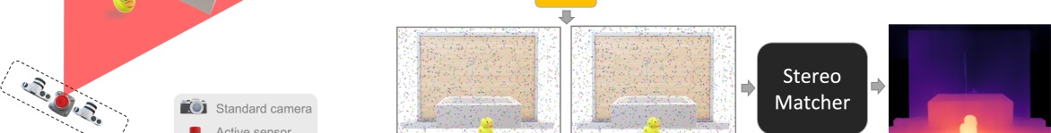
Figure 2: Overview of the proposed Virtual Pattern Projection framework. The envisioned setup on the left relies on a standard passive stereo camera and an active depth sensor. On the right, the step needed to obtain the coherently hallucinated stereo pair from the vanilla input images and sparse depth points through Virtual Pattern Projection (VPP). The patterned stereo pair in output can be processed by any stereo matcher, either handcrafted or learning-based.

2 Related Work

Stereo Matching. Traditional stereo algorithms [85, 72, 81, 80, 37, 65, 33, 27, 5], thoroughly investigated in [58], rely on handcrafted features and priors to compute dense disparity maps from stereo pairs. Deep learning has recently revolutionized stereo matching, providing significant improvements over conventional techniques on standard benchmarks [86]. Specifically, end-to-end stereo networks have become the most popular and effective solution for disparity estimation. These networks can be categorized into two main families: 2D and 3D architectures, with the former adopting an encoder-decoder design [46, 48, 38, 55, 62, 79, 82, 66], inspired by the U-Net model [54], while the latter build a feature cost volume from features extracted on the image pair and estimate the disparity map using 3D convolutions [30, 8, 32, 87, 12, 14, 19, 78, 74, 25, 61], at the cost of a much higher memory requirement and runtime. A complete review of such works can be found in [53]. More recent works [41, 35], instead, propose novel deep stereo networks that exploit the iterative refinement paradigm in the state-of-the-art optical flow network RAFT [67], or rely on Vision Transformers [36, 24] to capture long-range contextual information. Despite their superior performance, deep learning-based stereo methods require amounts of annotated data for training and yet suffer from limited generalization capabilities to unseen data [88, 6, 1, 90, 42, 16, 76, 71]. To alleviate this requirement, self-supervised techniques have been proposed to train deep stereo models without ground-truth annotations by relying on photometric losses on stereo pairs or videos [93, 70, 69, 34, 75, 15], traditional algorithms and confidence measures [68, 2]. Others propose self-supervised continual adaptation of stereo networks using images captured during deployment [70, 52].

Active Stereo Matching. Active stereo leverages a pattern projector, typically working in the IR spectrum, to ease the correspondence problem, particularly in low-textured and repetitive areas. These systems [9] rely on structured [23] or unstructured [31] light. A subclass of structured light systems – coded light – relies on spatial [26] or temporal coded patterns [84], with the latter struggling in the presence of moving objects at standard frame rate. Regardless of the technology, pattern projection is limited to shorter distances and is unsuitable for outdoor use with sunlight. Additionally, devices based on structured light patterns require carefully designed projectors and suffer from thermal drifts [21] among other issues [56]. Nonetheless, active stereo is a vivid research field [43, 20].

Image-Guided Methods. Another approach to estimating depth involves integrating sparse depth measurements from active sensors with RGB information. Specifically, two main trends are typically adopted in the literature.

Depth Completion. This approach aims to estimate dense depth maps from incomplete or noisy depth data or from a single RGB image combined with sparse depth measurements, which can be obtained from active sensors such as LiDAR or structured light. A wide range of methods have been proposed for this task, including traditional methods based on interpolation and optimization [7, 60, 44], as well as deep learning-based approaches [45, 11, 49, 28, 10, 40, 91]. However, these approaches typically suffer in estimating depth in regions with missing external depth values [18].

Guided Stereo Matching. In addition to advances in stereo matching, recent research has also explored the integration of stereo with active sensors. In Badino et al. [3], the authors propose to directly integrate LiDAR data into the stereo algorithm using dynamic programming. Gandhi et al. [22], instead, propose a method to fuse time-of-flight (ToF) camera and stereo pairs using an efficient seed-growing algorithm. More recent works, instead, exploit depth measurements, either by concatenating them as input of CNN-based architectures [13, 50, 89, 73] or by using them to guide the cost aggregation of existing cost volumes [51, 29, 92, 73]. Our approach augments the given stereo pair to enhance RGB images, providing more discriminative information to the network and making it easier to solve the correspondence problem, unlike other methods that only concatenate sparse depths or guide cost aggregation.

3 Virtual Pattern Projection (VPP)

This section describes our approach to ease visual correspondence across images acquired by a passive stereo camera by means of the coherent virtual projection of patterns leveraging the availability of reliable sparse depth points of the same scene. The motivation for enriching the visual image content of the original scene is the same as methods relying on a physical projector: it aims at increasing local distinctiveness to make the visual correspondence task more robust. However, in contrast to previous methods, our strategy follows an entirely different path discarding the need for a physical projector with all its mentioned limitations.

3.1 Virtual Projection Principle

Our proposal is based on the observation that given a rectified stereo rig, and availability of a set of sparse depth points registered with the reference image, each of these points implicitly allows us to determine the corresponding pixels in the stereo pair. Hence, by knowing this correspondence, we can augment the visual appearance of both pixels in the two images to make them as similar as possible and as distinctive as possible from their neighbors, as if an ideal smart virtual projector were sending its signal onto the sensed scene. Fig. 2 outlines our basic virtual projection principle, showing on the left the envisioned setup consisting of a calibrated stereo camera and a sensor performing sparse yet accurate depth estimation, registered with the stereo reference camera through an initial calibration. The vanilla stereo pair acquired by the passive cameras and the input depth map are shown at the top. Since the stereo rig and the active sensor are calibrated, the depth $z(x,y)$ of each sparse point allows us to locate corresponding points $I_{L}(x,y)$ and $I_{R}(x^{\prime},y)$ in the two input images. For this purpose, we transform $z(x,y)$ into a disparity $d(x,y)$ by knowing [64] the focal length $f$ and the baseline $b$ of the stereo camera with $d(x,y)=\frac{b\cdot f}{z(x,y)}$. Such a disparity value represents the offset needed to obtain the location along the same epipolar line of the corresponding point $I_{R}(x^{\prime},y)$ in the target image with $x^{\prime}=x-d(x,y)$. Fig. 2 shows how the two corresponding points A e B can be determined by knowing the depth of A in the input sparse depth map, and then we can augment them to achieve our goal.

Figure 3: Virtual patterns. From top to bottom: (i) indistinctive, (ii) randomly generated, (iii) distinctive, (iv) randomly generated patch-based uniform, (v) distinctive patch-based uniform, (vi) randomly generated patch-based, and (vii) distinctive patch-based patterns. For (iii), (v), and (vii) we report the search area of length $L$, set to 64 in our experiments, and height as depicted for $3\times 3$ virtual patterns.

3.2 Virtual Patterns

To properly hallucinate images and ease matching, corresponding points should be as similar as possible. Accordingly, we propose two augmenting strategies: random pattern and histogram-based pattern. Both operate on corresponding points $(x,y)$ and $(x^{\prime},y)$ located along the epipolar line with the same pattern $\mathcal{A}(x,x^{\prime},y)$ in the two images:

$$\begin{split}I_{L}(x,y)\leftarrow\mathcal{A}(x,x^{\prime},y)\\ I_{R}(x^{\prime},y)\leftarrow\mathcal{A}(x,x^{\prime},y)\end{split}$$ (1)

Their difference consists in how the operator $\mathcal{A}(x,x^{\prime},y)$ generates the virtual pattern superimposed on the input images. Fig. 3 outlines the several possible patterns that we will discuss in the remainder. Furthermore, as $x^{\prime}$ is unlikely to be an integer, $\mathcal{A}(x,x^{\prime},y)$ will apply to both $I_{R}(\lfloor x^{\prime}\rfloor,y)$ and $I_{R}(\lceil x^{\prime}\rceil,y)$ by means of a weighted splatting on the two.

$$\begin{split}I_{R}(\lfloor x^{\prime}\rfloor,y)\leftarrow\beta I_{R}(\lfloor x^{\prime}\rfloor,y)+(1-\beta)\mathcal{A}(x,x^{\prime},y)\\ I_{R}(\lceil x^{\prime}\rceil,y)\leftarrow(1-\beta)I_{R}(\lceil x^{\prime}\rceil,y)+\beta\mathcal{A}(x,x^{\prime},y)\end{split}$$ (2)

where $\beta=x^{\prime}-\lfloor x^{\prime}\rfloor$ is the splatting weight.

3.2.1 Random Patterning

To ease visual correspondence, the pattern should both increase similarity across images, as well as distinctiveness [83] along the epipolar line. As such, a pattern as the one shown in Fig. 3 (i) would be suboptimal. To address this issue, a method uses an operator $\mathcal{A}(x,x^{\prime},y)$ that samples a random value from a uniform distribution

$$\mathcal{A}(x,x^{\prime},y)\sim\mathcal{U}(0,255)$$ (3)

Fig. 3 (ii) depicts a possible outcome of this approach whose extension to color images, as for any method discussed, is straightforward by applying the same strategy on each color channel. This operator is fast and introduces distinctiveness to some degree, although not entirely. On the contrary, an operator taking into account the image content itself could enforce stronger distinctiveness [83].

3.2.2 Histogram-based Patterning

We argue that the patterns superimposed onto the vanilla image should stand out from the background and be unambiguous (at least) within nearby pixels along the same horizontal scanline, as depicted in Fig. 3 (iii).

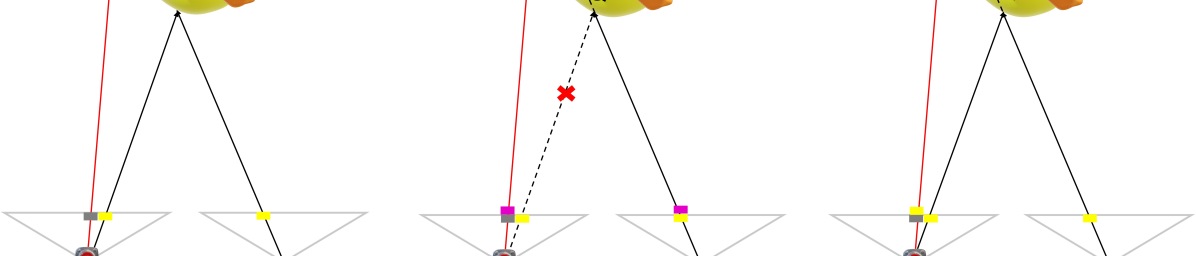
Figure 4: Handling occlusions. I) P is framed by the reference camera and depth sensor but occluded in the target camera (“NO” projection), II) Projection of the same pattern (violet) onto the two input images according to depth in the background (“BKGD”), III) Projection of the foreground image content (Q) from the target image to the background in the reference image (“FGD”).

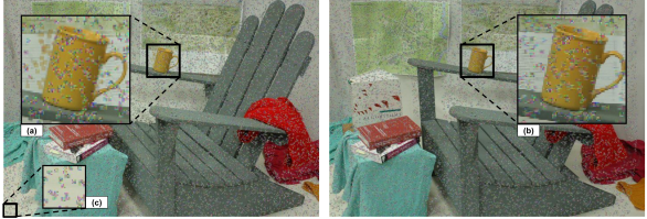
Figure 5: VPP in action. Hallucinated left and right images, zoomed-in view of the type (vi) pattern, showing FGD-Projection (a), corresponding area (b) with sub-pixel splatting and left border occlusion projection (c).

To achieve this goal, we employ a histogram-based operator $\mathcal{A}(x,x^{\prime},y)$, to select the pattern by analyzing the scanline content in the two hallucinated images. For $(x,y)$ in the reference image, we consider two windows of height 3 and length $L$ centered on it and on $(x^{\prime},y)$ in the target image. Then, the histograms computed over the two windows are summed up and the operator $\mathcal{A}(x,x^{\prime},y)$ picks the color maximizing the distance from any other color in the histogram $\text{hdist}(i)$, with $\text{hdist}(i)$ returning the minimum distance from a filled bin in the sum histogram $\mathcal{H}$

$$\begin{split}\text{hdist}(i)=&\big{\{}\min\{|i-i_{l}|,\,|i-i_{r}|\},\\ &i_{l}\in[0,i[:\mathcal{H}(i_{l})>0,\\ &i_{r}\in]i,255]:\mathcal{H}(i_{r})>0\big{\}}\end{split}$$ (4)

If every bin in $\mathcal{H}$ is filled, the color with minimum occurrence is selected.

3.3 Advanced Virtual Patterns

We now extend the strategies described so far, taking into account locality, the original image content, and occlusions.

3.3.1 Locality

The pointwise patterning strategy can be applied to larger areas to enhance the visual appearance further. To this purpose, we can extend previous methods to patches (e.g., $3\times 3$ or $5\times 5$), implicitly assuming the same disparity within these small regions. Fig. 3, in (iv) and (v), shows the outcome of the operator $\mathcal{A}(x,x^{\prime},y)$ that selects a uniform color within the patches according to, respectively, random sampling or a selection based on histograms in a larger region $L$. Further patterns can be generated by (vi) random sampling or (vii) histogram-base selection being performed for every pixel in the patch independently.

3.3.2 Alpha-Blending

Although a virtual pattern eases the match for traditional algorithms [27], it might hinder a deep stereo model not used to deal with it. Thus, we combine the original image content with the virtual pattern through alpha-blending [64] as follows, being $\alpha$ a hyperparameter:

$$\begin{split}I_{L}(x,y)\leftarrow(1-\alpha)I_{L}(x,y)+\alpha\mathcal{A}(x,x^{\prime},y)\\ I_{R}(x^{\prime},y)\leftarrow(1-\alpha)I_{R}(x^{\prime},y)+\alpha\mathcal{A}(x,x^{\prime},y)\end{split}$$ (5)

VPP	Hyperparameters				Error Rate (%) $>2$
	Pattern	$\alpha$	Patch	Occ.	RAFT-Stereo [41]	PSMNet [8]	rSGM
✗	✗	✗	✗	✗	11.5	29.3	34.3
✓	(ii)	✗	✗	BKGD	5.2	15.3	20.6
✓	(iii)	✗	✗	BKGD	5.1	15.2	20.2
✓	(ii)	0.4	✗	BKGD	5.8	16.7	21.2
✓	(iii)	0.4	✗	BKGD	5.6	16.1	20.5
✓	(iv)	0.4	$3\times 3$	BKGD	4.9	15.0	16.7
✓	(v)	0.4	$3\times 3$	BKGD	5.0	15.1	16.2
✓	(vi)	0.4	$3\times 3$	BKGD	5.0	15.3	15.9
✓	(vii)	0.4	$3\times 3$	BKGD	5.0	15.2	15.9
✓	(iv)	0.4	$3\times 3$	NO	4.9	14.7	16.2
✓	(v)	0.4	$3\times 3$	NO	4.9	14.8	15.7
✓	(vi)	0.4	$3\times 3$	NO	5.1	14.9	15.7
✓	(vii)	0.4	$3\times 3$	NO	4.9	14.9	15.4
✓	(iv)	0.4	$3\times 3$	FGD	4.8	14.4	16.1
✓	(v)	0.4	$3\times 3$	FGD	4.8	14.4	15.6
✓	(vi)	0.4	$3\times 3$	FGD	5.0	14.6	15.6
✓	(vii)	0.4	$3\times 3$	FGD	4.8	14.4	15.3

Table 1: Ablation on main projection hyperparameters. Results on Midd-A. Networks trained on synthetic data.

3.3.3 Occlusions

Since occluded regions inevitably exist in a stereo setup, even assuming a depth sensor perfectly aligned with the reference camera (although this is not always the case [17]), we might not be able to project the pattern consistently on the two views, as depicted in Fig. 4 I). Accordingly, it is crucial to detect points hitting occluded regions to avoid projecting the same pattern on both the occluded and the occluder pixels, respectively, on the reference and target images. Purposely, we devise a simple yet effective heuristic to classify sparse disparities warped onto the target image, according to the difference in disparity and spatial distance from other sparse points inferred by the sensor.

Specifically, we warp disparity $d$ for $(x,y)$ into an image-like grid $W$ at coordinates $(x^{\prime},y)$. In case of collisions – i.e., multiple $d$ warped at the same location $(x^{\prime},y)$ – the largest $d$ is kept. Then, each $(x_{o},y_{o})$ in $W$ is classified as occluded if the following inequality holds for at least one neighbor $W(x,y)$ within a $r_{x}\times r_{y}$ patch:

$$W(x,y)-W(x_{o},y_{o})-\lambda(\gamma\lvert x-x_{o}\rvert+(1-\gamma)\lvert y-y_{o}\rvert)>t$$ (6)

with $\lambda,\gamma,r_{x},r_{y},t$ being hyper-parameters. Finally, the occluded points are warped back to obtain a mask $o$.

When a depth point is classified as occluded, we can neglect projection on both reference and target images (“NO” projection strategy). This avoids projecting the same pattern on the foreground (in the target image) and background (in the reference), which would increase ambiguity at occlusions – “BKGD” projection strategy. Nonetheless, we follow a third strategy: we avoid projection and instead replace the original content in $(x,y)$ on the reference image with the content at $(x^{\prime},y)$ in the target image. This does not alter the appearance of the correct match on foreground (rays originating from Q), yet stimulates the stereo matcher to establish a second correspondence with the same point $(x^{\prime},y)$ in the target image, i.e., with pixel $(x,y)$ originating from P. This strategy will be referred to as “FGD” projection. Additionally, points in the left border of the reference image would project patterns outside the target. Although irrelevant for traditional algorithms, we still project there to avoid artifacts in the predictions by deep stereo networks. Fig. 5 shows an example of hallucinated pair.

4 Experimental Results

We describe our experimental setup, including implementation details, datasets, and results analysis.

			Midd-14					Midd-21					ETH3D
Model	Depth Points		Error Rate (%)				avg.	Error Rate (%)				avg.	Error Rate (%)				avg.
	Train	Test	$>1$	$>2$	$>3$	$>4$	(px)	$>1$	$>2$	$>3$	$>4$	(px)	$>1$	$>2$	$>3$	$>4$	(px)
rSGM [63]	✗	✗	69.97	41.86	29.41	25.19	13.62	67.33	40.55	27.69	22.37	8.02	27.20	9.11	5.64	4.26	1.18
rSGM-gd [51]	✗	✓	63.47	30.64	17.03	13.57	9.98	59.32	26.26	13.51	10.04	4.44	19.95	3.18	1.72	1.28	0.76
rSGM-vpp	✗	✓	57.98	20.37	10.86	9.49	7.81	52.81	15.08	6.63	5.51	3.40	9.66	0.62	0.46	0.41	0.58
PSMNet [8]	✗	✗	48.52	31.11	24.29	20.58	10.05	47.25	28.03	20.19	15.88	4.52	19.73	6.48	4.09	3.11	0.88
PSMNet-gd [51]	✗	✓	48.24	30.66	24.03	20.47	10.50	46.61	27.18	19.60	15.59	4.49	18.96	5.91	3.56	2.85	0.84
PSMNet-vpp	✗	✓	26.30	16.08	13.06	11.60	6.11	22.26	10.52	6.96	5.36	1.63	10.83	2.01	1.46	1.30	0.53
PSMNet-gd-ft [51]	✓	✓	33.82	15.61	10.74	8.77	4.52	35.76	13.77	7.55	5.21	1.71	12.28	2.43	0.86	0.61	0.54
PSMNet-vpp-ft	✓	✓	25.07	14.92	11.87	10.43	6.19	21.21	10.17	6.78	5.26	1.66	2.86	1.40	1.21	1.11	0.38
PSMNet-gd-tr [51]	✓	✓	25.17	12.61	9.13	7.59	3.84	23.67	9.63	5.75	4.15	1.33	4.79	0.85	0.54	0.42	0.33
PSMNet-vpp-tr	✓	✓	21.32	12.95	10.52	9.35	5.09	18.24	8.57	5.73	4.50	1.57	2.18	1.48	1.36	1.29	0.34
LidarStereoNet [13]	✓	✓	32.72	16.30	12.10	10.34	4.48	27.32	11.67	7.58	5.88	1.80	10.39	1.05	0.47	0.30	0.45
CCVNorm [73]	✓	✓	30.22	12.49	7.54	5.58	2.27	20.88	7.63	4.47	3.28	1.14	17.63	4.69	2.16	1.28	0.66
RAFT-Stereo [41]	✗	✗	24.24	15.65	12.48	10.62	3.87	20.05	10.28	7.18	5.55	1.31	2.84	1.44	0.90	0.74	0.28
RAFT-Stereo-gd [51]	✗	✓	24.14	11.58	7.85	6.08	2.87	20.38	8.31	5.09	3.65	1.11	5.32	1.68	1.06	0.76	0.41
RAFT-Stereo-vpp	✗	✓	8.04	5.30	4.35	3.81	2.01	6.94	4.26	3.33	2.78	0.72	1.30	0.83	0.65	0.54	0.15
RAFT-Stereo-gd-ft [51]	✓	✓	15.22	8.02	5.97	5.05	2.67	15.51	6.76	4.63	3.63	1.21	2.52	1.28	1.00	0.77	0.29
RAFT-Stereo-vpp-ft	✓	✓	7.12	4.73	3.95	3.51	1.95	6.40	4.00	3.20	2.76	0.83	1.01	0.74	0.64	0.58	0.14
RAFT-Stereo-gd-tr [51]	✓	✓	6.39	3.29	2.35	1.93	0.91	6.45	3.14	2.25	1.82	0.64	0.94	0.59	0.46	0.38	0.14
RAFT-Stereo-vpp-tr	✓	✓	5.57	4.14	3.63	3.33	1.51	4.85	3.05	2.39	2.01	0.66	0.71	0.57	0.51	0.47	0.12

Table 2: Comparison with existing methods. Results on Midd-14, Midd-21, ETH3D. Networks trained on synthetic data.

4.1 Implementation and Experimental Settings

All virtual pattern variants depicted in Fig. 3 from (ii) to (vii) are implemented in Cython, sub-pixel disparities splatted on adjacent pixels in the right view. Among the hyper-parameters, we set $\lambda=2,\gamma=0.4375,t=1$ and $r_{x}\times r_{y}=9\times 7$ for the occlusion detection heuristic, whose effectiveness is studied in the supplementary material. To assess the effectiveness of VPP, we run several experiments in comparison with existing approaches that combine sparse depth points with stereo algorithms and networks. In particular, we consider the Guided Stereo Matching framework [51], LidarStereoNet [13], and CCVNorm [73] as main competitors.

Since the first two approaches are implemented over the PSMNet [8] architecture, we apply VPP to PSMNet for a direct and fair comparison. However, the original PSMNet weights used in [51] yielded poor generalization results; therefore, we retrain it following the original protocol [8], i.e., for 10 epochs on SceneFlow with a constant learning rate equal to 1e-3. For fairness, LidarStereoNet and CCVNorm have been retrained using the same setting. Moreover, since guided stereo [51] represents our closest competitor – i.e., it can be applied without any architectural change to the stereo model – we implement it within a more modern network, RAFT-Stereo [41], and compare it against our VPP. To conclude, we extend this comparison with an implementation of the Semi-Global-Matching method [27], i.e., rSGM [63], as a representative of traditional stereo algorithms. We run it by setting the maximum disparity to 192 disparity P1=11, adaptive P2 [4] (with P2${}_{\text{min}}$=17, P2${}_{\alpha}=0.5$, P2${}_{\gamma}=35$), applying left-right check and a speckle filter to remove outliers, then filling holes with background interpolation [47].

4.2 Evaluation Datasets & Protocol

We run experiments on three indoor/outdoor datasets.

Middlebury. The Middlebury dataset [57] is a high-resolution stereo dataset featuring indoor scenes, captured under controlled lighting conditions with accurate ground-truth obtained using structured light. We evaluate our approach on three different splits: the Additional 13 scenes in Middlebury 2014 (Midd-A), the 15 scenes from Middlebury 2014 training set (Midd-14), and the 24 scenes from Middlebury 2021 (Midd-21). Results are evaluated at full resolution, with PSMNet models running at half and CCVNorm at quarter (Midd-14) and one third (Midd-21) resolution.

KITTI 2015 [47]. This real-world stereo dataset depicts autonomous driving scenarios, captured at a resolution of approximately 1280$\times$384 pixels with sparse ground-truth depth maps collected using a LiDAR sensor. It provides 200 stereo pairs annotated with ground-truth, including independently moving objects such as cars. Among the 200 samples, we select 142 stereo pairs for which raw LiDAR measurements are provided [13], allowing for evaluating VPP and competitors with data from a real sensor.

ETH3D [59]. This dataset collects indoor and outdoor scenes, with a total of 27 grayscale low-resolution stereo pairs and corresponding ground-truth disparity maps.

Evaluation Protocol. We compute the percentage of pixels with a disparity error higher than a certain threshold $\tau$, with respect to the ground-truth. We report error rates by varying $\tau$ to 1, 2, 3, and 4, together with the average disparity error (avg). We evaluate our computed disparity maps across both occluded and non-occluded regions with valid ground truth disparity unless otherwise noted.

4.3 Ablation Study

We start by studying the different pattern variants and components under different settings. Tab. 1 summarizes this ablation study, conducted on Midd-A at full resolution with PSMNet [8], RAFT-Stereo [41] and rSGM.

For each stereo pair, we randomly sample 5% sparse depth points from the dense ground-truth. Simply enabling virtual projection with pointwise virtual patterns (ii) and (iii), without explicit handling of occlusions, gives a massive boost in performance compared to the baseline, dropping the error rate to half for RAFT-Stereo (11 to 5%) and PSMNet (29 to 15%), while also reducing the error rate from 34 to 20% for rSGM. Adding alpha-blending with pointwise patterns yields similar, yet slightly worse results across all methods. Nonetheless, projecting patterns on $3\times 3$ patches in conjunction with alpha-blending enables additional and consistent improvements to all methods with virtual pattern (iv) the most effective except for rSGM, which is not surprisingly more effective with pattern (vii) since it builds the cost volume based on a pointwise cost function. By handling occlusions thanks to our heuristic, we obtain some further improvements when neglecting projection (“NO” strategy). Finally, enabling occlusion handling through the “FGD” strategy yields the best results for all methods, with slight differences among them with the four patch-based virtual patterns. Considering the outcome of the ablation, despite the slightly worse accuracy, we conduct the remaining experiments with virtual pattern vi) on $3\times 3$ patches, because of its a negligible computation overhead with respect to histogram-based projection, while enabling at the same time alpha-blending and “FGD” occlusion handling – i.e., in yellow in the table.

4.4 Comparison with Existing Approaches

We now assess the performance of VPP and its main competitors. If not differently specified, we randomly sample 5% depth points from ground-truth, as in [51].

Guided/VPP variants. Given the flexibility of both VPP and guided stereo, we evaluate their application to stereo networks under three different settings, respectively:

• Without retraining the stereo network (-gd/-vpp)

• After a brief fine-tuning of the pre-trained model, enhanced by guided or VPP frameworks (-gd-ft/-vpp-ft)

• By training from scratch a new model, enhanced by guided or VPP (-gd-tr/-vpp-tr)

For -ft variants, one epoch of finetuning is carried out on FlyingThings, with learning rate 1e-4 and 1e-5 for PSMNet and RAFT-Stereo, respectively. For -tr variants, PSMNet and RAFT-Stereo are trained for 10 and 20 epochs, with learning rates 1e-3 and 1e-4, respectively. In any case, PSMNet and RAFT-Stereo process $384\times 512$ and $360\times 720$ crops, respectively, with batch size 2 on a single 3090 GPU.

The three variants allow for evaluating guided stereo and VPP when deployed with the least effort – i.e., by simply taking a pre-trained stereo network off the shelf – or with deeper intervention by the developer, either through a short fine-tuning on the pre-existing model or, with major efforts, by retraining it from scratch.

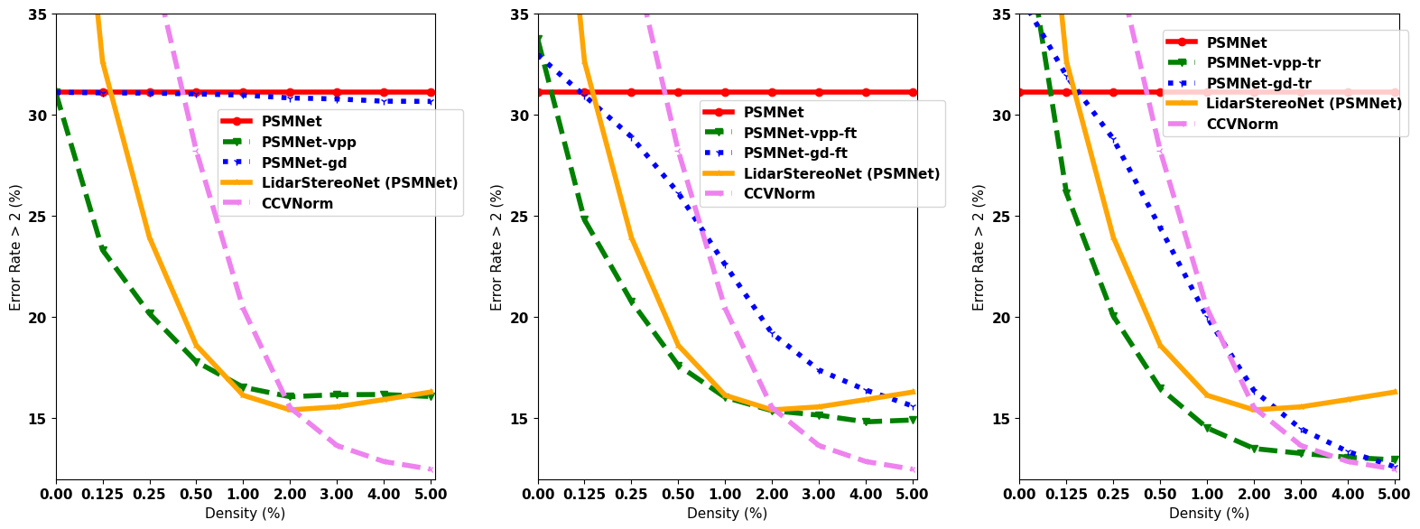
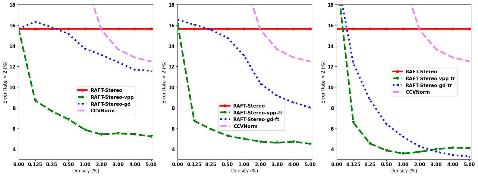
Figure 6: Depth sparsity vs accuracy. Results by VPP and competitors with different amounts of depth points.

			Midd-14
Model	Depth Points		Error Rate (%)				avg.
	Train	Test	$>1$	$>2$	$>3$	$>4$	(px)
rSGM [63]	✗	✗	69.97	41.86	29.41	25.19	13.62
rSGM-gd	✗	✓	63.47	30.64	17.03	13.57	9.98
rSGM-vpp	✗	✓	57.98	20.37	10.86	9.49	7.81
rSGM-gd-vpp	✗	✓	57.74	19.55	10.05	8.69	8.62
PSMNet [8]	✗	✗	48.52	31.11	24.29	20.58	10.05
PSMNet-gd	✗	✓	48.24	30.66	24.03	20.47	10.50
PSMNet-vpp	✗	✓	26.30	16.08	13.06	11.60	6.11
PSMNet-gd-vpp	✗	✓	27.68	16.49	13.44	12.00	6.30
LidarStereoNet [13]	✓	✓	32.72	16.30	12.10	10.34	4.48
LidarStereoNet-vpp	✓	✓	30.02	15.32	11.48	9.86	4.46
CCVNorm [73]	✓	✓	30.22	12.49	7.54	5.58	2.27
CCVNorm-vpp	✓	✓	28.29	12.26	7.42	5.51	2.20
RAFT-Stereo [41]	✗	✗	24.24	15.65	12.48	10.62	3.87
RAFT-Stereo-gd	✗	✓	24.14	11.58	7.85	6.08	2.87
RAFT-Stereo-vpp	✗	✓	8.04	5.30	4.35	3.81	2.01
RAFT-Stereo-gd-vpp	✗	✓	12.85	6.52	4.78	3.93	2.10

Table 3: Combining VPP with existing methods. Results on Midd-14, networks trained on synthetic data.

Comparison on Middlebury/ETH3D. Tab. 2 reports the outcome on Midd-14, Midd-21 and ETH3D datasets using models trained on synthetic data only or the rSGM algorithm. We can immediately notice one of the most prominent figures of merit of our proposal, i.e., the remarkable ability to largely boost cross-domain generalization on all datasets without any retraining of the pre-existing model (-vpp). On the contrary, guided stereo improves the results only marginally under this setting (-gd), while CCVNorm and LidarStereoNet need to be trained from scratch to process depth points (i.e., they are concatenated to RGB images). Accordingly, VPP is the undisputed winner in boosting the accuracy of stereo networks taken off the shelf.

By shortly fine-tuning the original networks to take advantage of sparse depth data is beneficial for both guided stereo (-gd-ft) and VPP (-vpp-ft) although the latter frequently, and always with RAFTStereo, outperforms the former even without any fine-tuning (-vpp), while training from scratch the networks to exploit the depth data with guided stereo (-gd-tr) results, sometimes, negligibly better than with VPP (-vpp-tr). This fact emphasizes further how VPP is much less training dependent, which is remarkable. Moreover, acting at the image level (VPP) is more robust than concatenating depth data to RGB (LidarStereoNet), acting on cost volumes (guided stereo) or both (CCVNorm).

			Midd-21
Model	Depth Points		Error Rate (%)				avg.
	Train	Test	$>1$	$>2$	$>3$	$>4$	(px)
PSMNet [8]	✗	✗	44.75	24.98	17.31	13.37	3.42
PSMNet-gd	✗	✓	44.40	24.58	16.98	13.09	3.40
PSMNet-vpp	✗	✓	21.38	10.32	6.85	5.24	1.51
PSMNet-gd-ft	✓	✓	40.47	16.06	8.56	5.83	1.78
PSMNet-vpp-ft	✓	✓	21.36	10.12	6.68	5.12	1.56
PSMNet-gd-tr	✓	✓	23.15	9.44	5.60	4.04	1.29
PSMNet-vpp-tr	✓	✓	18.07	8.64	5.79	4.51	1.50
LidarStereoNet [13]	✓	✓	25.08	10.09	6.47	4.94	1.86
CCVNorm [73]	✓	✓	20.54	7.45	4.31	3.12	1.06
RAFT-Stereo [41]	✗	✗	19.22	9.38	6.28	4.68	1.26
RAFT-Stereo-gd	✗	✓	18.82	6.95	4.06	2.88	1.05
RAFT-Stereo-vpp	✗	✓	6.65	4.00	3.10	2.60	0.71
RAFT-Stereo-gd-ft	✓	✓	14.87	6.09	3.99	3.09	1.02
RAFT-Stereo-vpp-ft	✓	✓	6.68	4.16	3.34	2.85	0.82
RAFT-Stereo-gd-tr	✓	✓	6.04	2.91	2.08	1.70	0.58
RAFT-Stereo-vpp-tr	✓	✓	4.76	3.00	2.39	2.02	0.69

Table 4: Results with fine-tuned models. Results on Midd-21, after fine-tuning on Midd-14.

			KITTI 142
Model	Depth Points		Error Rate (%)				avg.
	Train	Test	$>1$	$>2$	$>3$	$>4$	(px)
rSGM [63]	✗	✗	43.53	15.66	8.27	5.68	1.56
rSGM-gd	✗	✓	35.65	10.00	5.50	4.03	1.30
rSGM-vpp	✗	✓	23.56	6.12	4.04	3.20	1.17
PSMNet [8]	✗	✗	32.50	11.70	6.40	4.51	1.32
PSMNet-gd	✗	✓	32.59	11.94	6.71	4.81	1.35
PSMNet-vpp	✗	✓	20.94	6.85	4.24	3.26	1.06
PSMNet-gd-ft	✓	✓	30.39	9.79	5.18	3.69	1.27
PSMNet-vpp-ft	✓	✓	21.97	6.63	3.91	2.91	1.07
PSMNet-gd-tr	✓	✓	25.84	8.30	4.73	3.47	1.17
PSMNet-vpp-tr	✓	✓	17.60	5.96	3.86	3.01	1.03
LidarStereoNet [13]	✓	✓	33.01	10.16	5.13	3.57	1.33
CCVNorm [73]	✓	✓	18.98	6.78	4.50	3.52	1.17
RAFT-Stereo [41]	✗	✗	24.57	8.74	5.09	3.66	1.10
RAFT-Stereo-gd	✗	✓	32.50	12.61	7.10	4.95	1.33
RAFT-Stereo-vpp	✗	✓	15.36	6.33	4.31	3.37	0.92
RAFT-Stereo-gd-ft	✓	✓	23.90	8.37	5.01	3.72	1.13
RAFT-Stereo-vpp-ft	✓	✓	13.86	5.65	3.93	3.12	0.89
RAFT-Stereo-gd-tr	✓	✓	15.51	6.30	4.22	3.27	0.95
RAFT-Stereo-vpp-tr	✓	✓	11.64	4.78	3.46	2.80	0.87

Table 5: Experiments on KITTI. Results on the 142 split [13] with raw LiDAR. Networks trained on synthetic data.

				Midd-14					Midd-21					ETH3D					KITTI 142
		Depth Points		Error Rate (%)				avg.	Error Rate (%)				avg.	Error Rate (%)				avg.	Error Rate (%)				avg.
Model	Model name	Train	Test	$>1$	$>2$	$>3$	$>4$	(px)	$>1$	$>2$	$>3$	$>4$	(px)	$>1$	$>2$	$>3$	$>4$	(px)	$>1$	$>2$	$>3$	$>4$	(px)
RAFT-Stereo [41]	Middlebury	✗	✗	17.77	9.73	7.16	5.85	1.67	19.22	9.38	6.28	4.68	1.26	2.78	1.42	1.00	0.86	0.29	24.95	7.81	4.39	3.19	1.05
RAFT-Stereo-vpp	Middlebury	✗	✓	6.78	4.20	3.34	2.86	1.11	6.64	3.99	3.11	2.60	0.71	1.15	0.75	0.59	0.50	0.15	15.54	5.45	3.64	2.85	0.87
RAFT-Stereo [41]	ETH3D	✗	✗	24.70	16.25	13.09	11.35	4.82	20.25	10.18	7.09	5.48	1.39	2.61	1.26	0.94	0.76	0.27	24.42	8.62	4.99	3.64	1.09
RAFT-Stereo-vpp	ETH3D	✗	✓	8.16	5.34	4.34	3.79	2.28	6.81	4.08	3.17	2.70	0.72	1.24	0.77	0.60	0.51	0.14	15.16	6.22	4.23	3.31	0.92
GMStereo [77]	Sceneflow	✗	✗	50.13	29.15	20.19	15.67	4.10	44.60	23.04	15.88	12.44	2.59	6.43	2.51	1.67	1.13	0.39	30.17	10.46	5.54	3.85	1.20
GMStereo-vpp∗	Sceneflow	✗	✓	28.20	13.34	9.25	7.37	2.78	15.19	7.12	5.03	4.03	1.17	2.45	1.19	0.80	0.60	0.25	23.34	7.97	4.84	3.62	1.10
GMStereo [77]	Mixdata	✗	✗	28.50	12.60	7.88	5.81	1.51	21.10	7.34	4.37	3.16	0.98	1.72	0.31	0.11	0.07	0.28	17.00	4.03	2.20	1.46	0.73
GMStereo-vpp∗	Mixdata	✗	✓	18.32	7.81	5.40	4.23	1.34	11.19	4.57	3.09	2.35	0.75	1.13	0.38	0.21	0.14	0.25	13.71	3.82	2.23	1.56	0.67
CFNet [61]	Sceneflow	✗	✗	41.71	28.07	22.53	19.31	9.07	38.39	21.77	15.87	12.63	10.66	6.05	3.12	2.30	1.86	0.56	25.45	9.34	5.26	3.83	1.11
CFNet-vpp∗	Sceneflow	✗	✓	18.51	12.25	10.03	8.85	6.78	14.03	8.10	6.18	5.07	1.24	1.54	0.98	0.76	0.61	0.25	14.23	5.97	4.09	3.14	0.87
CFNet [61]	Middlebury	✗	✗	22.38	11.87	8.40	6.56	1.91	28.96	14.44	9.88	7.45	2.16	1.15	0.33	0.21	0.17	0.22	11.08	3.01	1.73	1.17	0.59
CFNet-vpp∗	Middlebury	✗	✓	13.16	8.12	6.33	5.36	1.79	11.83	6.92	5.23	4.28	1.00	0.75	0.33	0.25	0.20	0.17	8.66	2.69	1.67	1.18	0.53
HSMNet [82]	Middlebury	✗	✗	31.98	16.53	11.25	8.61	2.01	35.72	17.47	11.51	8.63	2.19	9.43	2.72	1.54	1.03	0.52	31.07	11.75	6.16	4.00	1.17
HSMNet-vpp	Middlebury	✗	✓	18.46	8.96	6.29	5.07	1.81	16.96	7.73	5.18	3.97	1.13	6.26	1.97	1.17	0.86	0.48	27.09	9.98	5.47	3.69	1.09
CREStereo [35]	ETH3D	✗	✗	19.80	9.99	7.01	5.44	1.51	21.81	9.86	6.76	5.38	1.36	1.54	0.51	0.32	0.22	0.19	21.97	7.26	4.21	3.07	0.98
CREStereo-vpp∗	ETH3D	✗	✓	12.84	7.08	5.31	4.40	1.42	9.46	5.69	4.39	3.64	1.03	1.17	0.69	0.50	0.39	0.13	14.76	5.88	3.90	2.96	0.85
LEAStereo [14]	Sceneflow	✗	✗	55.49	36.73	28.68	24.04	13.45	50.17	30.29	21.66	16.82	3.73	8.63	3.81	2.48	1.80	0.57	42.99	18.62	10.50	7.16	1.66
LEAStereo-vpp	Sceneflow	✗	✓	25.72	14.57	11.15	9.50	6.73	19.03	9.28	6.32	4.94	1.38	2.20	1.20	0.88	0.71	0.29	17.99	6.81	4.40	3.34	0.98
LEAStereo [14]	KITTI12	✗	✗	49.05	32.08	25.90	22.54	12.17	43.92	23.38	16.25	12.85	3.55	16.49	4.81	2.69	2.03	0.75	20.31	4.54	2.02	1.33	0.78
LEAStereo-vpp	KITTI12	✗	✓	29.17	15.36	12.52	11.31	8.11	22.01	10.09	7.45	6.21	1.90	11.89	2.84	1.66	1.28	0.51	11.98	3.12	1.81	1.27	0.63

Table 6: VPP with off-the-shelf networks. Results on Midd-14, Midd-21, ETH3D and KITTI. ^∗ uses $\alpha=0.2$ for blending.

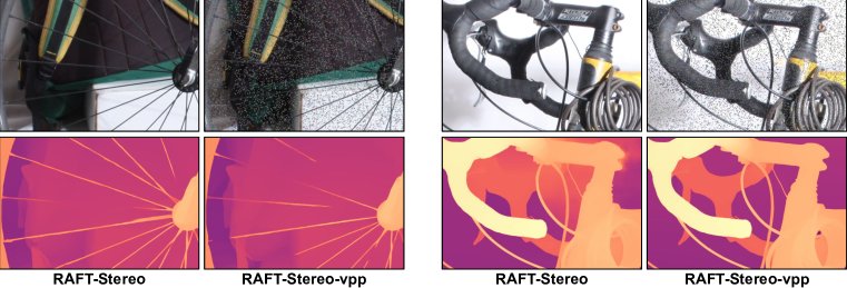
Figure 7: Performance by RAFT-Stereo-vpp on thin objects. Most fine details are preserved by VPP.

Depth Sparsity vs Accuracy. Fig. 6 shows the error rate ($>2$) on Midd-14 varying the density of sparse depth points from 0% to 5%. We can notice that VPP generally reaches almost optimal performance with a meagre 1% density and, except few cases in the -tr configurations with some higher density, achieves much lower error rates.

VPP + Existing Methods. Since our approach can be used seamlessly with other image-guided methods, Tab. 3 reports results yielded by such joint deployment on the Midd-14. VPP method alone is always more effective, except with rSGM, which benefits from joint deployment with guided stereo. Finally, using VPP with LidarStereoNet and CCVNORN also leads to slight improvements.

Results after Fine-Tuning on Real Data. Tab. 4 collects results analogous to those in Tab. 2, this time after having fine-tuned PSMNet and LidarStereoNet on Midd-14 for $\sim 4000$ steps [67], while for RAFT-Stereo we use the official Middlebury weights released by the authors. We observe a similar trend, with most VPP variants consistently outperforming the competitors, highlighting that VPP effectively improves cross-domain generalization as well as domain specialization.

Comparison on KITTI. To prove VPP accuracy with noisy depth data from a real sensor outdoor and at long-range where a physical pattern would be unusable, Tab. 5 reports experimental results on the KITTI 2015 dataset using raw LiDAR. The results confirm the previous trends: VPP constantly outperforms guided stereo – with any network and configuration – LidarStereoNet and CCVNorm.

VPP with More Off-the-shelf Networks. To conclude, Tab. 6 collects the results yielded VPP applied to several off-the-shelf stereo models [77, 61, 82, 35, 14], by running the weights provided by the authors. Again, VPP sensibly boosts the accuracy of any model with rare exceptions, either trained on synthetic or real data.

4.5 Qualitative results

To conclude, Fig. 7 shows qualitatively the effect of VPP on the predictions by RAFT-Stereo. We can appreciate how our virtual pattern can greatly enhance the quality of the disparity maps, without introducing relevant artefacts in correspondence of thin structures – despite applying the pattern on patches. More examples in the supplementary material.

5 Conclusion

This paper proposed a novel paradigm to achieve the robustness of active stereo without the need for a pattern projector with all its inherent limitations. Purposely, our technique replaces the projector with a generic depth sensor to obtain virtually hallucinated stereo pairs, greatly easing the visual correspondence task. Experimental results on standard stereo datasets highlight that our method achieves state-of-the-art performance with much higher flexibility, boosting the accuracy of stereo algorithms and networks.

Supplementary See pages 1 of paper-supp.pdf See pages 2 of paper-supp.pdf See pages 3 of paper-supp.pdf See pages 4 of paper-supp.pdf See pages 5 of paper-supp.pdf See pages 6 of paper-supp.pdf

References

- [1] Filippo Aleotti, Fabio Tosi, Pierluigi Zama Ramirez, Matteo Poggi, Samuele Salti, Stefano Mattoccia, and Luigi Di Stefano. Neural disparity refinement for arbitrary resolution stereo. In International Conference on 3D Vision, 2021. 3DV.
- [2] Filippo Aleotti, Fabio Tosi, Li Zhang, Matteo Poggi, and Stefano Mattoccia. Reversing the cycle: self-supervised deep stereo through enhanced monocular distillation. In 16th European Conference on Computer Vision (ECCV). Springer, 2020.
- [3] Hernán Badino, Daniel F. Huber, and Takeo Kanade. Integrating lidar into stereo for fast and improved disparity computation. 2011 International Conference on 3D Imaging, Modeling, Processing, Visualization and Transmission, pages 405–412, 2011.
- [4] Christian Banz, Peter Pirsch, and Holger Blume. Evaluation of penalty functions for semi-global matching cost aggregation. The International Archives of the Photogrammetry, Remote Sensing and Spatial Information Sciences; 39-B3, 39(B3):1–6, 2012.
- [5] Yuri Boykov, Olga Veksler, and Ramin Zabih. Fast approximate energy minimization via graph cuts. IEEE Transactions on pattern analysis and machine intelligence, 23(11):1222–1239, 2001.
- [6] Changjiang Cai, Matteo Poggi, Stefano Mattoccia, and Philippos Mordohai. Matching-space stereo networks for cross-domain generalization. In 2020 International Conference on 3D Vision (3DV), pages 364–373, 2020.
- [7] Massimo Camplani and Luis Salgado. Efficient spatio-temporal hole filling strategy for kinect depth maps. In Three-dimensional image processing (3DIP) and applications Ii, volume 8290, pages 127–136. SPIE, 2012.
- [8] Jia-Ren Chang and Yong-Sheng Chen. Pyramid stereo matching network. In IEEE/CVF Conference on Computer Vision and Pattern Recognition (CVPR), pages 5410–5418, 2018.
- [9] Rui Chen, Jing Xu, and Song Zhang. Comparative study on 3d optical sensors for short range applications. Optics and Lasers in Engineering, 149:106763, 2022.
- [10] Yun Chen, Bin Yang, Ming Liang, and Raquel Urtasun. Learning joint 2d-3d representations for depth completion. In Proceedings of the IEEE/CVF International Conference on Computer Vision, pages 10023–10032, 2019.
- [11] Xinjing Cheng, Peng Wang, and Ruigang Yang. Depth estimation via affinity learned with convolutional spatial propagation network. In Proceedings of the European Conference on Computer Vision (ECCV), pages 103–119, 2018.
- [12] Xinjing Cheng, Peng Wang, and Ruigang Yang. Learning depth with convolutional spatial propagation network. IEEE transactions on pattern analysis and machine intelligence, 42(10):2361–2379, 2019.
- [13] Xuelian Cheng, Yiran Zhong, Yuchao Dai, Pan Ji, and Hongdong Li. Noise-aware unsupervised deep lidar-stereo fusion. In Proc. IEEE Conf. Comp. Vis. Patt. Recogn., 2019.
- [14] Xuelian Cheng, Yiran Zhong, Mehrtash Harandi, Yuchao Dai, Xiaojun Chang, Hongdong Li, Tom Drummond, and Zongyuan Ge. Hierarchical neural architecture search for deep stereo matching. Advances in Neural Information Processing Systems, 33, 2020.
- [15] Cheng Chi, Qingjie Wang, Tianyu Hao, Peng Guo, and Xin Yang. Feature-level collaboration: Joint unsupervised learning of optical flow, stereo depth and camera motion. In Proceedings of the IEEE/CVF Conference on Computer Vision and Pattern Recognition, pages 2463–2473, 2021.
- [16] WeiQin Chuah, Ruwan Tennakoon, Reza Hoseinnezhad, Alireza Bab-Hadiashar, and David Suter. Itsa: An information-theoretic approach to automatic shortcut avoidance and domain generalization in stereo matching networks. In Proceedings of the IEEE/CVF Conference on Computer Vision and Pattern Recognition, pages 13022–13032, 2022.
- [17] Andrea Conti, Matteo Poggi, Filippo Aleotti, and Stefano Mattoccia. Unsupervised confidence for lidar depth maps and applications. In IEEE/RSJ International Conference on Intelligent Robots and Systems, 2022. IROS.
- [18] Andrea Conti, Matteo Poggi, and Stefano Mattoccia. Sparsity agnostic depth completion. In Proceedings of the IEEE/CVF Winter Conference on Applications of Computer Vision (WACV), pages 5871–5880, January 2023.
- [19] Shivam Duggal, Shenlong Wang, Wei-Chiu Ma, Rui Hu, and Raquel Urtasun. Deeppruner: Learning efficient stereo matching via differentiable patchmatch. In Proceedings of the IEEE/CVF international conference on computer vision, pages 4384–4393, 2019.
- [20] Sean Ryan Fanello, Julien Valentin, Christoph Rhemann, Adarsh Kowdle, Vladimir Tankovich, Philip Davidson, and Shahram Izadi. Ultrastereo: Efficient learning-based matching for active stereo systems. In 2017 IEEE Conference on Computer Vision and Pattern Recognition (CVPR), pages 6535–6544, 2017.
- [21] David Fiedler and Heinrich Müller. Impact of thermal and environmental conditions on the kinect sensor. In Xiaoyi Jiang, Olga Regina Pereira Bellon, Dmitry Goldgof, and Takeshi Oishi, editors, Advances in Depth Image Analysis and Applications, pages 21–31, Berlin, Heidelberg, 2013. Springer Berlin Heidelberg.
- [22] Vineet Gandhi, Jan Čech, and Radu Horaud. High-resolution depth maps based on tof-stereo fusion. In 2012 IEEE International Conference on Robotics and Automation, pages 4742–4749. IEEE, 2012.
- [23] Jason Geng. Structured-light 3d surface imaging: a tutorial. Adv. Opt. Photon., 3(2):128–160, Jun 2011.
- [24] Weiyu Guo, Zhaoshuo Li, Yongkui Yang, Zheng Wang, Russell H Taylor, Mathias Unberath, Alan Yuille, and Yingwei Li. Context-enhanced stereo transformer. In Proceedings of the European Conference on Computer Vision (ECCV), 2022.
- [25] Xiaoyang Guo, Kai Yang, Wukui Yang, Xiaogang Wang, and Hongsheng Li. Group-wise correlation stereo network. In Proceedings of the IEEE/CVF Conference on Computer Vision and Pattern Recognition, pages 3273–3282, 2019.
- [26] Jungong Han, Ling Shao, Dong Xu, and Jamie Shotton. Enhanced computer vision with microsoft kinect sensor: A review. IEEE Transactions on Cybernetics, 43(5):1318–1334, 2013.
- [27] Heiko Hirschmuller. Stereo processing by semiglobal matching and mutual information. IEEE Transactions on pattern analysis and machine intelligence, 30(2):328–341, 2007.
- [28] Mu Hu, Shuling Wang, Bin Li, Shiyu Ning, Li Fan, and Xiaojin Gong. Penet: Towards precise and efficient image guided depth completion. In 2021 IEEE International Conference on Robotics and Automation (ICRA), pages 13656–13662. IEEE, 2021.
- [29] Yu-Kai Huang, Yueh-Cheng Liu, Tsung-Han Wu, Hung-Ting Su, Yu-Cheng Chang, Tsung-Lin Tsou, Yu-An Wang, and Winston H Hsu. S3: Learnable sparse signal superdensity for guided depth estimation. In Proceedings of the IEEE/CVF Conference on Computer Vision and Pattern Recognition, pages 16706–16716, 2021.
- [30] Alex Kendall, Hayk Martirosyan, Saumitro Dasgupta, Peter Henry, Ryan Kennedy, Abraham Bachrach, and Adam Bry. End-to-end learning of geometry and context for deep stereo regression. In The IEEE International Conference on Computer Vision (ICCV), Oct 2017.
- [31] Leonid Keselman, John Iselin Woodfill, Anders Grunnet-Jepsen, and Achintya Bhowmik. Intel realsense stereoscopic depth cameras. In Proceedings of the IEEE Conference on Computer Vision and Pattern Recognition (CVPR) Workshops, July 2017.
- [32] Sameh Khamis, Sean Fanello, Christoph Rhemann, Adarsh Kowdle, Julien Valentin, and Shahram Izadi. Stereonet: Guided hierarchical refinement for real-time edge-aware depth prediction. In Proceedings of the European Conference on Computer Vision (ECCV), pages 573–590, 2018.
- [33] Vladimir Kolmogorov and Ramin Zabin. What energy functions can be minimized via graph cuts? IEEE transactions on pattern analysis and machine intelligence, 26(2):147–159, 2004.
- [34] Hsueh-Ying Lai, Yi-Hsuan Tsai, and Wei-Chen Chiu. Bridging stereo matching and optical flow via spatiotemporal correspondence. In Proceedings of the IEEE/CVF Conference on Computer Vision and Pattern Recognition, pages 1890–1899, 2019.
- [35] Jiankun Li, Peisen Wang, Pengfei Xiong, Tao Cai, Ziwei Yan, Lei Yang, Jiangyu Liu, Haoqiang Fan, and Shuaicheng Liu. Practical stereo matching via cascaded recurrent network with adaptive correlation. In Proceedings of the IEEE/CVF Conference on Computer Vision and Pattern Recognition, pages 16263–16272, 2022.
- [36] Zhaoshuo Li, Xingtong Liu, Nathan Drenkow, Andy Ding, Francis X Creighton, Russell H Taylor, and Mathias Unberath. Revisiting stereo depth estimation from a sequence-to-sequence perspective with transformers. In Proceedings of the IEEE/CVF International Conference on Computer Vision, pages 6197–6206, 2021.
- [37] Chia-Kai Liang, Chao-Chung Cheng, Yen-Chieh Lai, Liang-Gee Chen, and Homer H Chen. Hardware-efficient belief propagation. IEEE Transactions on Circuits and Systems for Video Technology, 21(5):525–537, 2011.
- [38] Zhengfa Liang, Yiliu Feng, Yulan Guo, Hengzhu Liu, Wei Chen, Linbo Qiao, Li Zhou, and Jianfeng Zhang. Learning for disparity estimation through feature constancy. In Proceedings of the IEEE Conference on Computer Vision and Pattern Recognition (CVPR), June 2018.
- [39] Juan-Ting Lin, Dengxin Dai, and Luc Van Gool. Depth estimation from monocular images and sparse radar data. In International Conference on Intelligent Robots and Systems (IROS), 2020.
- [40] Yuankai Lin, Tao Cheng, Qi Zhong, Wending Zhou, and Hua Yang. Dynamic spatial propagation network for depth completion. In Proceedings of the AAAI Conference on Artificial Intelligence, volume 36, pages 1638–1646, 2022.
- [41] Lahav Lipson, Zachary Teed, and Jia Deng. Raft-stereo: Multilevel recurrent field transforms for stereo matching. In International Conference on 3D Vision (3DV), 2021.
- [42] Biyang Liu, Huimin Yu, and Guodong Qi. Graftnet: Towards domain generalized stereo matching with a broad-spectrum and task-oriented feature. In Proceedings of the IEEE/CVF Conference on Computer Vision and Pattern Recognition, pages 13012–13021, 2022.
- [43] I. Liu, E. Yang, J. Tao, R. Chen, X. Zhang, Q. Ran, Z. Liu, and H. Su. Activezero: Mixed domain learning for active stereovision with zero annotation. Proceedings of the IEEE/CVF Conference on Computer Vision and Pattern Recognition, 2022.
- [44] Si Lu, Xiaofeng Ren, and Feng Liu. Depth enhancement via low-rank matrix completion. In Proceedings of the IEEE conference on computer vision and pattern recognition, pages 3390–3397, 2014.
- [45] Fangchang Ma, Guilherme Venturelli Cavalheiro, and Sertac Karaman. Self-supervised sparse-to-dense: Self-supervised depth completion from lidar and monocular camera. In 2019 International Conference on Robotics and Automation (ICRA), pages 3288–3295. IEEE, 2019.
- [46] Nikolaus Mayer, Eddy Ilg, Philip Hausser, Philipp Fischer, Daniel Cremers, Alexey Dosovitskiy, and Thomas Brox. A large dataset to train convolutional networks for disparity, optical flow, and scene flow estimation. In The IEEE Conference on Computer Vision and Pattern Recognition (CVPR), June 2016.
- [47] Moritz Menze and Andreas Geiger. Object scene flow for autonomous vehicles. In Conference on Computer Vision and Pattern Recognition (CVPR), 2015.
- [48] Jiahao Pang, Wenxiu Sun, Jimmy SJ. Ren, Chengxi Yang, and Qiong Yan. Cascade residual learning: A two-stage convolutional neural network for stereo matching. In The IEEE International Conference on Computer Vision (ICCV), Oct 2017.
- [49] Jinsun Park, Kyungdon Joo, Zhe Hu, Chi-Kuei Liu, and In So Kweon. Non-local spatial propagation network for depth completion. In Computer Vision–ECCV 2020: 16th European Conference, Glasgow, UK, August 23–28, 2020, Proceedings, Part XIII 16, pages 120–136. Springer, 2020.
- [50] Kihong Park, Seungryong Kim, and Kwanghoon Sohn. High-precision depth estimation with the 3d lidar and stereo fusion. In 2018 IEEE International Conference on Robotics and Automation (ICRA), pages 2156–2163. IEEE, 2018.
- [51] Matteo Poggi, Davide Pallotti, Fabio Tosi, and Stefano Mattoccia. Guided stereo matching. In Proceedings of the IEEE/CVF Conference on Computer Vision and Pattern Recognition, pages 979–988, 2019.
- [52] Matteo Poggi, Alessio Tonioni, Fabio Tosi, Stefano Mattoccia, and Luigi Di Stefano. Continual adaptation for deep stereo. IEEE Transactions on Pattern Analysis and Machine Intelligence (TPAMI), 2021.
- [53] Matteo Poggi, Fabio Tosi, Konstantinos Batsos, Philippos Mordohai, and Stefano Mattoccia. On the synergies between machine learning and binocular stereo for depth estimation from images: A survey. IEEE Transactions on Pattern Analysis and Machine Intelligence, 44(9):5314–5334, 2022.
- [54] Olaf Ronneberger, Philipp Fischer, and Thomas Brox. U-net: Convolutional networks for biomedical image segmentation. In Medical Image Computing and Computer-Assisted Intervention–MICCAI 2015: 18th International Conference, Munich, Germany, October 5-9, 2015, Proceedings, Part III 18, pages 234–241. Springer, 2015.
- [55] Tonmoy Saikia, Yassine Marrakchi, Arber Zela, Frank Hutter, and Thomas Brox. Autodispnet: Improving disparity estimation with automl. In Proceedings of the IEEE/CVF International Conference on Computer Vision, pages 1812–1823, 2019.
- [56] Hamed Sarbolandi, Damien Lefloch, and Andreas Kolb. Kinect range sensing: Structured-light versus time-of-flight kinect. Computer Vision and Image Understanding, 139:1–20, 2015.
- [57] Daniel Scharstein, Heiko Hirschmüller, York Kitajima, Greg Krathwohl, Nera Nešić, Xi Wang, and Porter Westling. High-resolution stereo datasets with subpixel-accurate ground truth. In German conference on pattern recognition, pages 31–42. Springer, 2014.
- [58] Daniel Scharstein and Richard Szeliski. A taxonomy and evaluation of dense two-frame stereo correspondence algorithms. Int. J. Comput. Vis., 47(1-3):7–42, 2002.
- [59] Thomas Schöps, Johannes L. Schönberger, Silvano Galliani, Torsten Sattler, Konrad Schindler, Marc Pollefeys, and Andreas Geiger. A multi-view stereo benchmark with high-resolution images and multi-camera videos. In Conference on Computer Vision and Pattern Recognition (CVPR), 2017.
- [60] Ju Shen and Sen-Ching S Cheung. Layer depth denoising and completion for structured-light rgb-d cameras. In Proceedings of the IEEE conference on computer vision and pattern recognition, pages 1187–1194, 2013.
- [61] Zhelun Shen, Yuchao Dai, and Zhibo Rao. Cfnet: Cascade and fused cost volume for robust stereo matching. In Proceedings of the IEEE/CVF Conference on Computer Vision and Pattern Recognition (CVPR), pages 13906–13915, June 2021.
- [62] Xiao Song, Xu Zhao, Hanwen Hu, and Liangji Fang. Edgestereo: A context integrated residual pyramid network for stereo matching. In ACCV, 2018.
- [63] Robert Spangenberg, Tobias Langner, Sven Adfeldt, and Raúl Rojas. Large scale semi-global matching on the cpu. In 2014 IEEE Intelligent Vehicles Symposium Proceedings, pages 195–201. IEEE, 2014.
- [64] Richard Szeliski. Computer Vision - Algorithms and Applications, Second Edition. Texts in Computer Science. Springer, 2022.
- [65] Tatsunori Taniai, Yasuyuki Matsushita, and Takeshi Naemura. Graph cut based continuous stereo matching using locally shared labels. In Proceedings of the IEEE Conference on Computer Vision and Pattern Recognition, pages 1613–1620, 2014.
- [66] Vladimir Tankovich, Christian Hane, Yinda Zhang, Adarsh Kowdle, Sean Fanello, and Sofien Bouaziz. Hitnet: Hierarchical iterative tile refinement network for real-time stereo matching. In Proceedings of the IEEE/CVF Conference on Computer Vision and Pattern Recognition (CVPR), pages 14362–14372, June 2021.
- [67] Zachary Teed and Jia Deng. Raft: Recurrent all-pairs field transforms for optical flow. In European conference on computer vision, pages 402–419. Springer, 2020.
- [68] Alessio Tonioni, Matteo Poggi, Stefano Mattoccia, and Luigi Di Stefano. Unsupervised adaptation for deep stereo. In The IEEE International Conference on Computer Vision (ICCV). IEEE, Oct 2017.
- [69] Alessio Tonioni, Oscar Rahnama, Tom Joy, Luigi Di Stefano, Ajanthan Thalaiyasingam, and Philip Torr. Learning to adapt for stereo. In The IEEE Conference on Computer Vision and Pattern Recognition (CVPR). IEEE, June 2019.
- [70] Alessio Tonioni, Fabio Tosi, Matteo Poggi, Stefano Mattoccia, and Luigi Di Stefano. Real-time self-adaptive deep stereo. In The IEEE Conference on Computer Vision and Pattern Recognition (CVPR). IEEE, June 2019.
- [71] Fabio Tosi, Alessio Tonioni, Daniele De Gregorio, and Matteo Poggi. Nerf-supervised deep stereo. In Conference on Computer Vision and Pattern Recognition (CVPR), pages 855–866, June 2023.
- [72] Olga Veksler. Stereo correspondence by dynamic programming on a tree. In 2005 IEEE Computer Society Conference on Computer Vision and Pattern Recognition (CVPR’05), volume 2, pages 384–390. IEEE, 2005.
- [73] Tsun-Hsuan Wang, Hou-Ning Hu, Chieh Hubert Lin, Yi-Hsuan Tsai, Wei-Chen Chiu, and Min Sun. 3d lidar and stereo fusion using stereo matching network with conditional cost volume normalization. In 2019 IEEE/RSJ International Conference on Intelligent Robots and Systems (IROS), pages 5895–5902. IEEE, 2019.
- [74] Yan Wang, Zihang Lai, Gao Huang, Brian H Wang, Laurens Van Der Maaten, Mark Campbell, and Kilian Q Weinberger. Anytime stereo image depth estimation on mobile devices. In 2019 International Conference on Robotics and Automation (ICRA), pages 5893–5900, 2019.
- [75] Yang Wang, Peng Wang, Zhenheng Yang, Chenxu Luo, Yi Yang, and Wei Xu. Unos: Unified unsupervised optical-flow and stereo-depth estimation by watching videos. In Proceedings of the IEEE Conference on Computer Vision and Pattern Recognition, pages 8071–8081, 2019.
- [76] Jamie Watson, Oisin Mac Aodha, Daniyar Turmukhambetov, Gabriel J. Brostow, and Michael Firman. Learning stereo from single images. In European Conference on Computer Vision (ECCV), 2020.
- [77] Haofei Xu, Jing Zhang, Jianfei Cai, Hamid Rezatofighi, Fisher Yu, Dacheng Tao, and Andreas Geiger. Unifying flow, stereo and depth estimation. arXiv preprint arXiv:2211.05783, 2022.
- [78] Gengshan Yang, Joshua Manela, Michael Happold, and Deva Ramanan. Hierarchical deep stereo matching on high-resolution images. In Proceedings of the IEEE/CVF Conference on Computer Vision and Pattern Recognition, pages 5515–5524, 2019.
- [79] Guorun Yang, Hengshuang Zhao, Jianping Shi, Zhidong Deng, and Jiaya Jia. Segstereo: Exploiting semantic information for disparity estimation. In ECCV, pages 636–651, 2018.
- [80] Qingxiong Yang, Liang Wang, and Narendra Ahuja. A constant-space belief propagation algorithm for stereo matching. In 2010 IEEE Computer Society Conference on Computer Vision and Pattern Recognition, pages 1458–1465. IEEE, 2010.
- [81] Qingxiong Yang, Liang Wang, Ruigang Yang, Henrik Stewénius, and David Nistér. Stereo matching with color-weighted correlation, hierarchical belief propagation, and occlusion handling. IEEE transactions on pattern analysis and machine intelligence, 31(3):492–504, 2008.
- [82] Zhichao Yin, Trevor Darrell, and Fisher Yu. Hierarchical discrete distribution decomposition for match density estimation. In Proceedings of the IEEE/CVF Conference on Computer Vision and Pattern Recognition, pages 6044–6053, 2019.
- [83] Kuk-Jin Yoon and In-So Kweon. Stereo matching with the distinctive similarity measure. In ICCV, pages 1–7. IEEE Computer Society, 2007.
- [84] Aviad Zabatani, Vitaly Surazhsky, Erez Sperling, Sagi Ben Moshe, Ohad Menashe, David H. Silver, Zachi Karni, Alexander M. Bronstein, Michael M. Bronstein, and Ron Kimmel. Intel® realsense™ sr300 coded light depth camera. IEEE Transactions on Pattern Analysis and Machine Intelligence, 42(10):2333–2345, 2020.
- [85] Ramin Zabih and John Woodfill. Non-parametric local transforms for computing visual correspondence. In Third European Conference on Computer Vision (Vol. II), 3rd European Conference on Computer Vision (ECCV), pages 151–158, Secaucus, NJ, USA, 1994. Springer-Verlag New York, Inc.
- [86] Jure Zbontar, Yann LeCun, et al. Stereo matching by training a convolutional neural network to compare image patches. J. Mach. Learn. Res., 17(1):2287–2318, 2016.
- [87] Feihu Zhang, Victor Prisacariu, Ruigang Yang, and Philip HS Torr. GA-Net: Guided aggregation net for end-to-end stereo matching. In IEEE/CVF Conference on Computer Vision and Pattern Recognition (CVPR), 2019.
- [88] Feihu Zhang, Xiaojuan Qi, Ruigang Yang, Victor Prisacariu, Benjamin Wah, and Philip Torr. Domain-invariant stereo matching networks. In Europe Conference on Computer Vision (ECCV), 2020.
- [89] Junming Zhang, Manikandasriram Srinivasan Ramanagopal, Ram Vasudevan, and Matthew Johnson-Roberson. Listereo: Generate dense depth maps from lidar and stereo imagery. In 2020 IEEE International Conference on Robotics and Automation (ICRA), pages 7829–7836. IEEE, 2020.
- [90] Jiawei Zhang, Xiang Wang, Xiao Bai, Chen Wang, Lei Huang, Yimin Chen, Lin Gu, Jun Zhou, Tatsuya Harada, and Edwin R Hancock. Revisiting domain generalized stereo matching networks from a feature consistency perspective. In Proceedings of the IEEE/CVF Conference on Computer Vision and Pattern Recognition, pages 13001–13011, 2022.
- [91] Youmin Zhang, Xianda Guo, Matteo Poggi, Zheng Zhu, Guan Huang, and Stefano Mattoccia. Completionformer: Depth completion with convolutions and vision transformers. In Proceedings of the IEEE/CVF Conference on Computer Vision and Pattern Recognition, pages 18527–18536, 2023.
- [92] Yongjun Zhang, Siyuan Zou, Xinyi Liu, Xu Huang, Yi Wan, and Yongxiang Yao. Lidar-guided stereo matching with a spatial consistency constraint. ISPRS Journal of Photogrammetry and Remote Sensing, 183:164–177, 2022.
- [93] Yiran Zhong, Yuchao Dai, and Hongdong Li. Self-supervised learning for stereo matching with self-improving ability. arXiv:1709.00930, 2017.
See pages 1 of paper-supp.pdf See pages 2 of paper-supp.pdf See pages 3 of paper-supp.pdf See pages 4 of paper-supp.pdf See pages 5 of paper-supp.pdf See pages 6 of paper-supp.pdf