Constraining dark energy cosmologies with spatial curvature using Supernovae JWST forecasting

Abstract

Recent cosmological tensions, in particular, to infer the local value of the Hubble constant $H_{0}$, have developed new independent techniques to constrain cosmological parameters in several cosmologies. Moreover, even when the concordance Cosmological Constant Cold Dark Matter ($\Lambda$CDM) model has been well constrained with local observables, its physics has shown deviations from a flat background. Therefore, to explore a possible deviation from a flat $\Lambda$CDM model that could explain the $H_{0}$ value in tension with other techniques, in this paper we study new cosmological constraints in spatial curvature dark energy models. Additionally, to standard current Supernovae Type Ia (SNIa) catalogs, we extend the empirical distance ladder method through an SNIa sample using the capabilities of the James Webb Space Telescope (JWST) to forecast SNIa up to $z\sim 6$, with information on the star formation rates at high redshift. Furthermore, we found that our constraints provide an improvement in the statistics associated with $\Omega_{m}$ when combining SNIa Pantheon and SNIa Pantheon+ catalogs with JW forecasting data.

1 Introduction

The first direct evidence of the late time cosmic acceleration was obtained through measurements of Type Ia Supernovae (SNIa) [1, 2]. Over the years, subsequent observations confirmed this result, such as the cosmic microwave background (CMB) [3], baryon acoustic oscillations (BAO) [4, 5], and weak gravitational lensing [6]. However, the capability of supernovae to prove the accelerating expansion remains invaluable since these objects are bright enough to be seen at large distances. Furthermore, SNIa are common enough to be found in large quantities, and their properties make them standardized with a precision of $\sim 0.1$ mag in brightness or $\sim 5\%$ in distance per object [7]. Also, the increasing number of SNIa observations has considerably reduced the associated statistical errors and the uncertainties in estimating cosmological parameters dominated by them [8, 9].

Nevertheless, the nature of this cosmic acceleration is one of the current inquiries in precision cosmology since still we do not fully understand the component with which it is associated, the dark energy. However, due to the well-constrained $\Lambda$-Cold Dark Matter ($\Lambda$CDM) model, this dark energy could be evidence for a component with a negative Equation–of–State (EoS) constant value [10, 11, 12] or a dynamical EoS [13, 14, 15]. Furthermore, dark energy can be associated with components that can be derived from first principles in alternative theories of gravity [16, 17, 18] and extended theories of gravity [19, 20], showing a late cosmic acceleration.

On the nature of dark energy, several missions have been working to find better cosmological constraints adjoint with better systematics and increasing data baselines. Some of them as large-scale structure (LSS) observations with measurements from the Dark Energy Survey (DES) [21], the Dark Energy Spectroscopic Instrument (DESI) [22], the Legacy Survey of Space and Time (LSST) on the Vera Rubin Observatory [23], and Euclid [24], among others, have extended the concordance cosmological model to include EoS parameters of dark energy with some shifts within 1$\sigma$.

In particular, the recently launched James Webb Space Telescope (JWST) is a very interesting experiment that can help to elucidate the nature of dark energy. JWST is a 6.5-meter primary mirror, space-based observatory operating in the visible and infrared light equipped with four main science instruments including a near-infrared camera, spectrograph, and imager slitless spectrograph; and a mid-infrared camera and spectrograph [25]. It is expected that it will have an estimated lifespan of 20 years in which the research will be focused on several astrophysical and cosmology areas such as galaxy formation in the early universe as [26, 27, 28, 29], exoplanet detection [30, 31, 32], metallicity and chemical exploration [33, 34, 35], and life detection [36, 37]. All these potential and current observations could allow us to explore physics further than before as testing dark energy models with structure formation [38, 39], corroborate the Cepheid calibrations in the distance ladder [40] and adding more SNIa observations [9], cosmic chronometers [41], and XA/UV quasars [42, 43] to the constraint analysis of them.

Recently, numerous studies related to the implications of JWST to cosmology have been developed. In [9] a JWST simulated sample of SNIa within a redshift range $2\lesssim z\lesssim 6$, was employed to constrain standard cosmological parameters. Using combinations of the mock sample and SN Pantheon dataset [44] it was possible to constrain dark energy models with constant EoS. This analysis was performed using two different forms of the intrinsic evolution of the standardized SNIa luminosity distance. On one hand, it is assumed a linear redshift dependence of magnitude evolution. On the other hand, we can consider other logarithmic evolutions. Analysing the cases with and without systematic evolution, it was found that the addition of the simulated SNIa sample would successfully remove the evolutionary effects. However, even though the SN Pantheon dataset size was increased by a factor of $\approx$ 16 data points, it is still not able to constrain the systematic evolution and the cosmological parameters as effectively as the very high redshift SN data.

A further study about the first galaxies discovered by JWST was carried out in [45]. According to several works [46, 47, 48, 49, 50, 51, 52], there are some common aspects within the structure morphology, which indicate that galaxies discovered by JWST do not have enough time to evolve into what it is observed today. It is important to notice that this study is within the framework of the standard cosmological $\Lambda$CDM model. Therefore, the new JWST dataset includes near and mid-infrared images and near-infrared spectra to perform analyses based on cosmographic theories of the angular size-redshift relationship [45]. The $\Lambda$CDM interpretation of JWST observations is compared with the interpretation based on Zwicky’s static universe model [53], where the origin of the cosmological redshift can be explained through the photon-energy loss mechanism. However, the redshifted objects detected by the JWST are not aligned with such interpretation, but before any final conclusion, data from this mission should be increased.

As a step forward, using the capabilities of the JWST described, in this work, we develop the forecasting of SNIa up to $z\sim 6$, with information on the Star Formation Rates (SFR) at high redshift. Once this data is at hand, we perform a statistical analysis combined with SN Pantheon [44] and SN Pantheon+ to constrain spatial curvature dark energy cosmologies. We based our cosmological models inspired by bidimensional EoS parameterisation, which preserves the expanding and accelerating behaviour at late times. Our goal is to show that a simple deviation in the spatial curvature of a dark energy EoS model can verify a well-constrained analysis with SNIa JWST forecasting.

This paper is divided as follows: In Sec. 2 we summarise the theory behind dark energy bidimensional parameterisations inspired in Taylor series around the cosmological scale factor $a$. All of these parameterisations are described through their normalised $E(z)$ Friedmann evolution equation, including the curvature term. Furthermore, we are going to consider standard $\Lambda$CDM and $w$CDM models in addition to the dark energy cosmologies to proceed with comparisons between them. Also, we include the latest constraints reported in the literature so far. In Sec. 3 we present the methodology employed for observables. We include the description of current SNIa data baselines and how we can proceed with their forecasting using JWST characteristics. In Appendix A we describe the technicalities behind this forecasting. The results on new constraints for the models described are developed in Sec. 4. Finally, the conclusions are presented in Sec. 5.

2 Standard dark energy parameterisations

The standard cosmological scenario $\Lambda$CDM is a remarkable fit for most cosmological data. Nonetheless, we are still searching for the nature of inflation, dark matter, and dark energy. Physical evidence for these components comes only from astrophysical and cosmological observations [54]. Therefore, an increase in experimental sensitivity can produce deviations from the standard $\Lambda$CDM scenario that could lead to a deeper understanding of the gravity theory. If it is not a consequence associated with systematic errors, the cosmological tensions [55] existing between the different experimental probes could indicate a failure of the $\Lambda$CDM model, and a better cosmological model should be able to be found.

In this section, we are going to describe, in addition to the $\Lambda$CDM model with EoS $w=-1$, five dark energy bidimensional in $z$ parameterisations of $w(z)$, which can be constant or redshift-dependent. Notice that to describe dark energy, we need to achieve cosmic acceleration with a negative pressure at late times [11].

• $\Lambda$CDM model. In this model, the universe is composed of cosmological fluids with different EoS’s $w$ that contribute to the energy constraint. At present cosmic times, the non-relativistic matter contribution, $\Omega_{m}\simeq 0.27$, is the sum of the ordinary baryonic matter term, $\Omega_{b}\simeq 0.044$, and the (cold) dark matter term, $\Omega_{c}\simeq 0.22$. Dark energy ($\Omega_{\Lambda}\simeq 0.73$) is described by $w=-1$, associated with a cosmological constant $\Lambda$ or a vacuum energy density [56]. Radiation represents a negligible contribution, $\Omega_{r}\simeq 9\times 10^{-5}$, but it dominated the early cosmic stages, after the end of the inflationary stage and before matter-radiation decoupling [57]. Additionally, $\Lambda$CDM can be characterized with a flat geometry, which corresponds to an energy density parameter, $\Omega_{\Lambda}=1-\Omega_{m}-\Omega_{r}$, where the only parameter to be constrained is $\Omega_{m}$. The cosmological evolution for this model can be expressed as

  $$E(z)\equiv\dfrac{H(z)}{H_{0}}=\sqrt{\Omega_{m}(1+z)^{3}+\Omega_{r}(1+z)^{4}+\Omega_{\Lambda}},$$ (2.1)

  where $H_{0}$ is the Hubble constant today.

  We also consider the non-flat $\Lambda$CDM cosmological model, as an extension of the $\Lambda$CDM model but with curvature $k\neq 0$, with its constraint equation as $\Omega_{k}=1-\Omega_{m}-\Omega_{r}-\Omega_{\Lambda}$, where $\Theta=(\Omega_{m},\Omega_{\Lambda})$ is the vector with free parameters. The evolution for this case can be written as

  $$E(z)=\sqrt{\Omega_{m}(1+z)^{3}+\Omega_{r}(1+z)^{4}+\Omega_{k}(1+z)^{2}+\Omega_{\Lambda}}.$$ (2.2)

  Then, the model-dependent luminous distance can be calculated according to the $\Omega_{k}$ value [58]:

  $$D_{L}(z)=\left\{\begin{array}[]{ll}\dfrac{c}{H_{0}}(1+z)\dfrac{\sinh{\left(\sqrt{\Omega_{k}}\int_{0}^{z}\dfrac{dz^{\prime}}{E(z^{\prime})}\right)}}{\sqrt{\Omega_{k}}},&\quad\quad\Omega_{k}>0\\ \dfrac{c}{H_{0}}(1+z)\int_{0}^{z}\dfrac{dz^{\prime}}{E(z^{\prime})},&\quad\quad\Omega_{k}=0\\ \dfrac{c}{H_{0}}(1+z)\dfrac{\sin{\left(\sqrt{-\Omega_{k}}\int_{0}^{z}\dfrac{dz^{\prime}}{E(z^{\prime})}\right)}}{\sqrt{-\Omega_{k}}},&\quad\quad\Omega_{k}<0,\end{array}\right.$$ (2.3)

  where $c$ the speed of light and $E(z)$ the background evolution equation of the cosmological models.

  The base test for $\Lambda$CDM is the analysis provided by the Planck collaboration measuring CMB anisotropies finding the base parameters values $\Omega_{m}=0.316\pm 0.008$ and $H_{0}=67.27\pm 0.6$ km s^-1 Mpc^-1 [59] in the context of a flat $\Lambda$CDM. Using late-time data in [58] was found that using SNIa, BAO, and a quasar sample the values are $\Omega_{m}=0.300\pm 0.012$, with a fixed $H_{0}=70$ km s^-1 Mpc^-1, while using a non-flat $\Lambda$CDM model the results were $\Omega_{m}=0.364\pm 0.021$ and $\Omega_{\Lambda}=0.829\pm 0.035$, finding a slight deviation from the flat background. Furthermore, with a Cosmic Chronometers (CC – $H(z)$) sample it was found that $H_{0}=66.7\pm 5.3$ km s^-1 Mpc^-1 and $\Omega_{m}=0.33^{+0.08}_{-0.06}$ for the same flat model [60]. Using only SNIa Pantheon+ compilation [7] the values for the flat $\Lambda$CDM model are $H_{0}=73.6\pm 1.1$ km s^-1 Mpc^-1. The latter assumes a Gaussian prior with $\Omega_{m}=0.334\pm 0.018$. While for the non-flat $\Lambda$CDM the results are $\Omega_{m}=0.306\pm 0.057$ and $\Omega_{\Lambda}=0.625\pm 0.084$ in concordance with the flat counterpart at $2\sigma$.

• $w$CDM model. The simplest extension of the $\Lambda$CDM model is the one in which $w\neq-1$, yet still constant in time meaning that $w(z)=w_{0}$. From [9, 58] we express $E(z)$ for this model as,

  $$E(z)=\sqrt{\Omega_{m}(1+z)^{3}+\Omega_{k}(1+z)^{2}+\Omega_{\Lambda}(1+z)^{3(1+w_{0})}}.$$ (2.4)

  Non-flat $w$CDM has $\Theta=(\Omega_{m},\Omega_{\Lambda},w_{0})$ as free parameters. However, under flatness assumption, $\Omega_{k}$ = 0, so the only free parameters are $\Theta=(\Omega_{m},w_{0})$. This model reduces to $\Lambda$CDM when $w_{0}=-1$.

  Using SNIa, BAO, and quasars the values obtained in [58] were: $\Omega_{m}=0.369^{+0.022}_{-0.023}$ and $w_{0}=-1.283^{+0.094}_{-0.027}$, corresponding to a deviation from the $\Lambda$CDM model in more than $1\sigma$ range with the same fixed $H_{0}$ value. While using a non-flat $w$CDM results in $\Omega_{m}=0.280^{+0.041}_{-0.037}$, $\Omega_{\Lambda}=1.662^{+0.041}_{-0.048}$ and $w_{0}=-0.667^{+0.024}_{-0.027}$, where a difference from a flat model is reported of more than $3\sigma$ using only SNIa and quasars. Furthermore, adding BAO to the quasar sample [61] results in $\Omega_{m}=0.31\pm 0.03$ and $w_{0}=-1.00^{+0.14}_{-0.13}$, that is consistent with $\Lambda$CDM assuming a Gaussian prior of $H_{0}=67.32\pm 4.7$ km s^-1 Mpc^-1. When using only SNIa [7] the flat $w$CDM model gives $\Omega_{m}=0.309^{+0.063}_{-0.069}$, $H_{0}=73.5\pm 1.1$ km s^-1 Mpc^-1 and $w_{0}=-0.90\pm 0.14$, returning the confirmation for a $\Lambda$CDM model.

• Chevallier–Polarski–Linder (CPL) model. One of the most used redshift-dependent parameterisations corresponds to the Chevallier-Polarski-Linder [62, 63] proposal: $w(z)=w_{0}+w_{a}z/(1+z)$. In which, $w(z)=w_{0}+w_{a}$ at $z=\infty$ and $w(z)=w_{0}$ at $z=0$, but it diverges in the future for $z\rightarrow(-1)^{+}$. In this bidimensional model, $w_{0}$ denotes the dark energy EoS today, and $w_{a}$ describes its evolution. This parameterisation has several advantages including the well behaviour at high redshift, the linear feature at low redshift, a simple physical interpretation, and the accuracy in reconstructing a scalar field EoS [63]. The normalised Hubble parameter for this model can be written as

  $$E(z)=\sqrt{\Omega_{m}(1+z)^{3}+\Omega_{k}(1+z)^{2}+\Omega_{\Lambda}(1+z)^{3(1+w_{0}+w_{a})}\exp(\dfrac{-3w_{a}z}{1+z})}.$$ (2.5)

  For the non-flat and flat cases, we consider as free parameters ($\Omega_{m}$, $\Omega_{\Lambda}$, $w_{0}$, $w_{a}$) and ($\Omega_{m}$, $w_{0}$, $w_{a}$), respectively. This model can be reduced to $\Lambda$CDM with $w_{0}=-1$ and $w_{a}=0$.

  Using SNIa, BAO, and quasars in [58] was discussed a deviation from the $\Lambda$CDM with $\Omega_{m}=0.354^{+0.032}_{-0.030}$, along with $w_{0}=-1.323^{+0.103}_{0.112}$ and $w_{a}=0.745^{+0.483}_{-0.974}$ for a flat CPL model, values that correspond to a confirmation of the $\Lambda$CDM model. Using quasars and $H(z)$ measurements for a non-flat CPL parametrization it was found that $\Omega_{m}=0.44\pm 0.10$, $\Omega_{k}=-0.36\pm 0.24$, $H_{0}=71.8^{+4.6}_{-7.7}$, with $w_{0}=-1.2\pm 1.0$, and $w_{a}=-5.0^{+9-0}_{-2.0}$ [64] showing a clear deviation of more than $2\sigma$ from the flat $\Lambda$CDM model. Using SNIa [7] for the flat CPL with a Gaussian prior in $H_{0}$ results in $H_{0}=73.3\pm 1.1$ km s^-1 Mpc^-1, with $\Omega_{m}=0.403^{+0.054}_{-0.098}$, $w_{0}=-0.93\pm 0.15$ and $w_{a}=-0.1^{+0.9}_{-2.0}$. This latter corresponds to a flat $\Lambda$CDM confirmation. Furthermore, adding BAO, CMB to the previous SNIa sample results in $H_{0}=67.41^{+0.52}_{-0.82}$ km s^-1 Mpc^-1, $\Omega_{m}=0.316^{+0.009}_{-0.005}$ and $w_{0}=1.267^{+0.196}_{-0.191}$ and $w_{a}=-3.771^{+2.113}_{-2.496}$ [58].

• Jassal-Bagla-Padmanabhan (JBP) model. In [65] the parameterisation $w(z)=w_{0}+w_{a}z/(1+z)^{2}$, in which $w(0)=w_{0}$, $w^{\prime}(0)=w_{1}$, and $w(\infty)=w_{0}$ is presented based on trying to explain the accelerated universe covering both CMB and the SNIa measurements. This model was proposed to solve the high $z$ issues within the CPL parameterisation [11]. Using the behaviour of this function allows us to have the same EoS at the present epoch and high-$z$ with a rapid variation at small redshifts. Considering the corresponding term related to curvature, the derivative expression for $E(z)$ for this model can be written as

  $$E(z)=\sqrt{\Omega_{m}(1+z)^{3}+\Omega_{k}(1+z)^{2}+\Omega_{\Lambda}(1+z)^{3(1+w_{0})}\exp[\dfrac{3w_{a}z^{2}}{2(1+z)^{2}}]},$$ (2.6)

  where $\Theta=(\Omega_{m},\Omega_{\Lambda},w_{0},w_{a})$ for the non-flat JBP model, and $\Theta=(\Omega_{m},w_{0},w_{a})$ for a flat JBP model.

  Using SNIa, BAO, and quasars the JBP model is tested obtaining $\Omega_{m}=0.354^{+0.032}_{-0.030}$, $w_{0}=-1.371\pm 0.141$ and $w_{a}=1.127^{+1.293}_{-1.547}$ [58] which is considered a deviation from the confirmation for $\Lambda$CDM for the $w_{0}$ value. In [66] using SNIa, BAO, CMB and Gamma-Ray Bursts (GRB) it is obtained $\Omega_{m}=0.27\pm 0.03$ with $w_{0}=-1.02\pm 0.04$ and $w_{a}=0.22\pm 0.23$ using a flat JBP model in concordance with a flat $\Lambda$CDM at $1\sigma$.

• Exponential model. In [67] was examined five one-parameter dark energy parameterisations with several datasets. In particular, data from CMB observations, Joint light-curve analysis from SNIa observations (JLA), BAO distance measurements, and $H(z)$. It was concluded that the one-parameter dark energy model can provide a solution to the $H_{0}$ tension between local measurements and Planck indirect ones. Besides, it was found which of the five models is better fitted to the data used. This model, relatively close to $\Lambda$CDM, is the one with an EoS of the form: $w(z)=w_{0}\exp[z/(1+z)]/(1+z)$, where $w(0)=w_{0}$ and $w(z)=0$, for both $z=\infty$ and $z\rightarrow(-1)^{+}$. As a result, the normalised Hubble parameter can be written as

  $$E(z)=\sqrt{\Omega_{m}(1+z)^{3}+\Omega_{k}(1+z)^{2}+\Omega_{\Lambda}(1+z)^{3}\exp[3w_{0}\left(\exp(\dfrac{z}{1+z})-1\right)]}.$$ (2.7)

  For non-flat exponential model we have $\Theta=(\Omega_{m},\Omega_{\Lambda},w_{0})$, while for flat exponential model, $\Theta=(\Omega_{m},w_{0})$.

  Using SNIa, quasars, and BAO was obtained for the Exponential model $\Omega_{m}=0.359^{+0.023}_{-0.024}$ and $w_{0}=-1.271^{+0.092}_{-0.107}$ [58] showing again a deviation from a flat $\Lambda$CDM. In [68] the exponential model is constrained using CMB, SNIa, BAO, and measurements of the distance using Hydrogen II galaxies resulting in $H_{0}=70.9\pm 7.0$ km s^-1 Mpc^-1, $\Omega_{m}=0.284\pm 0.006$ and $w_{0}=-1.202^{+0.027}_{-0.026}$, imposing a Gaussian local prior in $H_{0}$.

• Barboza-Alcaniz (BA) model. In [69] was proposed a dark energy parameterization given by $w(z)=w_{0}+w_{a}z(1+z)/1+z^{2}$. This is a well-behaved function of redshift throughout the entire cosmic evolution, $z\in[-1,\infty]$, with $w(z)=w_{0}+w_{a}$ for $z=\infty$ and $w(z)=w_{0}$, when $z\rightarrow(-1)^{+}$. This smooth function allows to define regions on the plane $(w_{0}-w_{1})$ associated with several classes of dark energy models to exclude or confirm the models based on the constraints using observational data. Thus, it was shown that both quintessence and phantom behaviors have fully acceptable regimes. The $E(z)$ for non-flat case of this model can be written as

  $$E(z)=\sqrt{\Omega_{m}(1+z)^{3}+\Omega_{k}(1+z)^{2}+\Omega_{\Lambda}(1+z)^{3(1+w_{0})}\left(1+z^{2}\right)^{\frac{3w_{a}}{2}}}.$$ (2.8)

  The free parameter sets for the non-flat BA model and flat BA model are $\Theta=(\Omega_{m},\Omega_{\Lambda},w_{0},w_{a})$ and $\Theta=(\Omega_{m},w_{0},w_{a})$, respectively. The analysis using BAO, SNIa and quasars in [58] showed deviation from the flat $\Lambda$CDM as $\Omega_{m}=0.307^{+0.044}_{-0.055}$, $w_{0}=-1.303^{+0.115}_{-0.106}$ and $w_{a}=1.010^{+0.152}_{-0.466}$, meaning that the quasar sample is responsible for a deviation from the standard model. In [66] using CMB, BAO, SNIa and GRB results in $\Omega_{m}=0.28\pm 0.03$, $w_{0}=-1.13\pm 0.04$ and $w_{a}=0.37\pm 0.1$, finding a lower deviation from the $\Lambda$CDM model, but using only BAO and CMB the standard model is recovered with $\Omega_{m}=0.29\pm 0.04$, $w_{0}=-1.06\pm 0.11$ and $w_{a}=0.35\pm 0.12$.

3 Data treatment: observations and forecastings

In this section, we will perform the statistical analysis for the dark energy models with and without curvature including three different datasets: SNIa Pantheon and SNIa Pantheon+ samples, along with the extracted simulated data from JWST.

• Pantheon (PN) [44]: The Pantheon compilation is a combination of measurements from SNIa distances combining both low and high redshifts from $z\sim 0.01$ up to $z=2.26$. This sample has shown an improvement in the photometric calibrations on the distance ladder through the light curve. This transforms observable quantities into distances adding up to a total of 1048 data points.

• Pantheon+ (PN⁺) [70, 71]: Pantheon+ is a collection of 18 different SNIa samples based on the Pantheon compilation above described and by adding new data points recollected from different surveys as: Foundation Supernova Survey [72], the Swift Optical/Ultraviolet Supernova Archive (SOUSA) [73], the Lick Observatory Supernova Search LOSS1 [74], the second sample LOSS2 [75], and DES [70]. As a result, Pantheon+ consists of 1701 light curves of 1550 distinct SNIa along a redshift of $z=$ 0.001 up to 2.26. For $H_{0}$, a value of $73.30\pm 1.04$ km s^-1 Mpc^-1 is assumed. This sample is represented in Figure 1 in blue color. Cosmological parameter constraints have been carried out using the affine-invariant ensemble sampler for Markov Chain Monte Carlo (MCMC) module emcee that uses random generation numbers to explore the parameter space based on the probability function $P\propto\exp(-\chi^{2}/2)$ to minimize the quantity

  $$\chi^{2}_{\text{SNIa}}(\Theta)=\Delta\mu^{T}(z,\Theta)\cdot C^{-1}_{\text{SNIa}}\cdot\Delta\mu(z,\Theta)+\ln{\left(\dfrac{S}{2\pi}\right)},$$ (3.1)

  where $\Delta\mu(z,\Theta)=\mu(z)_{\text{data}}-\mu(z,\Theta)_{\text{model}}$, $C_{\text{SNIa}}$ is the covariance matrix of the PN (or PN+) sample, $S$ is the sum of all the components of $C^{-1}_{\text{SNIa}}$, $\mu(z)_{\text{data}}$ is the distance modulus of the PN (PN+) data, and $\mu(z,\Theta)_{\text{model}}$ is the distance modulus for a cosmological model with a parameter set $\Theta$ [76].

• The extracted JWST simulated SN data (JW) [9]: Recently it was created an SNIa sample at $z>2$ using a Monte Carlo simulation derived from the capabilities of JWST and based on the FLARE project [77, 78]. The SNIa redshifts (up to $z\sim 6$) were derived by extrapolating the local supernovae rates with information on SFR at high redshift [79]. With this survey, in 6 years we expect to measure 205 SNIa in a range of $z\sim 0.3$ up to $z\sim 6$. We represent this sample in Figure 1. The mock sample was created based on a flat-$\Lambda$CDM model using a fit from Pantheon data. To develop our analysis, we changed the sample for SN PN⁺. The full covariance matrix is constructed by adding the off-diagonal value of $0.002^{2}$ with + and – signs assigned randomly for all the matrix. The value in the diagonal is the mean value of the Pantheon covariance matrix [8] and the $0.15^{2}$ value in the diagonal is the assumed error considering the local determination of the observation errors extrapolated [9]. The covariance matrix has the following form

  $$C_{\text{JW}}=\underbrace{\begin{pmatrix}\ 0.15^{2}&\pm 0.002^{2}&\pm 0.002^{2}&\dots&\pm 0.002^{2}\ \hbox{}\\ \ \pm 0.002^{2}&0.15^{2}&\pm 0.002^{2}&\dots&\pm 0.002^{2}\ \hbox{}\\ \ \pm 0.002^{2}&\pm 0.002^{2}&0.15^{2}&\dots&\pm 0.002^{2}\ \hbox{}\\ \ \vdots&\vdots&\vdots&\ddots&\vdots\ \hbox{}\\ \ \pm 0.002^{2}&\dots&\dots&\dots&0.15^{2}\ \\ \end{pmatrix}}_{\begin{subarray}{c}\\[1.39998pt] \text{\normalsize$n\times n$}\end{subarray}},$$ (3.2)

  where $n\times n$ denotes the dimension of the matrix and ($\pm$) the random assignment of (+) and (–) signs. In this case,

  $$\chi^{2}_{\text{JW}}(\Theta)=\Delta\mu^{T}(z,\Theta)\cdot C^{-1}_{\text{JW}}\cdot\Delta\mu(z,\Theta)+\ln{\left(\dfrac{S}{2\pi}\right)},$$ (3.3)

  where $\Delta\mu(z,\Theta)=\mu(z)_{\text{data}}-\mu(z,\Theta)_{\text{model}}-\Gamma_{0}$, $C_{\text{JW}}$ is the covariance matrix presented in Eq.(3.2), $S$ is the sum of all the components of $C^{-1}_{\text{JW}}$, $\mu(z)_{\text{data}}$ is the distance modulus of the JW data, $\mu(z,\Theta)_{\text{model}}$ is the distance modulus for a cosmological model with parameter set $\Theta$ and $\Gamma_{0}$ is a magnitude bias added to consider a possible systematic luminosity difference between the JW and PN (PN+) datasets. Notice that if we compare our Eq.(3.3) with [9], the analysis does not consider logarithmic systematics in the forecasting.

  For more technical details about the methodology followed here see Appendix A.

  

  

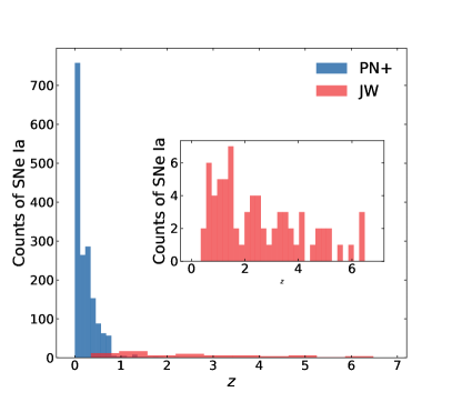
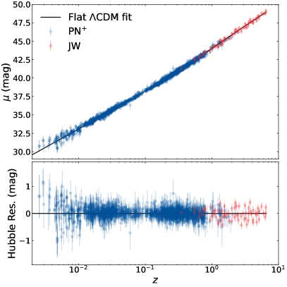
  Figure 1: Left: Histogram of the Pantheon+ data (blue) and the extracted JW (red). Right: Hubble Diagram of the Pantheon data (blue) and the extracted mock JW (red).

4 Results: Cosmological constraints

In this section, we discuss the constraints for the dark energy models previously described. In Tables 1 and 2 are reported the values for the cosmological parameters involved in each flat and non-flat model, respectively. Additionally, we used the results from the latest SH0ES measurement for the Hubble constant [71] in which using the local distance ladder via Cepheid calibration was obtained $H_{0}=73.04\pm 1.04$, and was introduced as a fixed value for the Hubble constant in our analyses. Also, an absolute magnitude $M=-19.263$ was assumed, except for flat $\Lambda$CDM where $M$ was taken as a free parameter. The optimal constraints on the cosmological parameters were derived using the emcee code. All Confidence Levels (C.L) presented in this work correspond to 68.3 and 95 $\%$ i.e., to 1 and 2$\sigma$ respectively. Finally, in the presented results the value of $\Omega_{k}$ is calculated directly from $\Omega_{k}=1-\Omega_{m}-\Omega_{\Lambda}$, combining the marginalized distributions of each fractional density using a getdist modified version.

4.1 $\Lambda$CDM model

The constraints for this model are given in Figure 2. As we can notice, using the Pantheon sample gives a relatively lower value of $\Omega_{m}$ than using the Pantheon+ sample for the flat-$\Lambda$CDM model. Comparing $\Omega_{m}=0.290\pm 0.008$ with $\Omega_{m}=0.311^{+0.010}_{-0.009}$, shows a tendency due to the addition of JW data. Furthermore, considering the non-flat model results in a higher $\Omega_{m}$ estimation for the Pantheon+ sample.

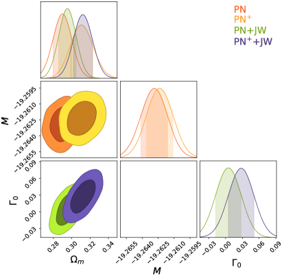
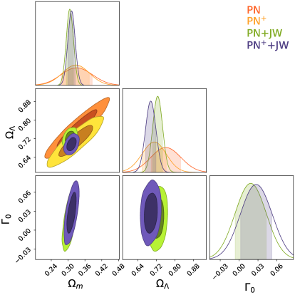
Figure 2: 1-2$\sigma$ C.L results for the $\Lambda$CDM model using SNIa Pantheon–PN (red color), SNIa Pantheon+–PN⁺ (orange color), SNIa Pantheon & JW mock data – PN+JW (green color) and SNIa Pantheon+ & JW mock data – PN⁺+JW (purple color) baselines: Left: Flat case. Right: Non-flat case. Notice that the C.L for $M$ is not associated with $\Gamma_{0}$.

The non-flat $\Lambda$CDM model constrained by JW simulated data tends to reduce the curvature estimation towards flatness $\Omega_{k}\sim 0$. Let us keep in mind that the results on curvature constraints are negative for all four different dataset combinations. There is a deviation from a flat universe with $\Omega_{k}=-0.0092\pm 0.0091$ using the Pantheon compilation. Additionally, the flat $\Lambda$CDM model constrains $\Gamma_{0}$ for the JW mock sample lower than $\Gamma_{0}=0.028\pm 0.018$ mag, which implies that there is no significant difference expected for the calibrated sample.

4.2 $w$CDM model

The constraints for this model are given in Figure 3. As we can notice, there is a correlation between the $w_{0}$ and $\Omega_{m}$ values present in the flat model, while in the non-flat version of the model, this vanishes and for the Pantheon and JW datasets there is a high error determination in the $w_{0}-\Omega_{m}$ parameter space. For this model, the fractional matter density has a similar value using Pantheon and Pantheon+ with the introduction of JW as $\Omega_{m}\sim 0.333$. The curvature estimation is closer to $\Omega_{k}=0$ as expected using the JW simulated data for the flat model. Furthermore, notice that we have a $1\sigma$ deviation from a flat model using only the Pantheon+ sample of $\Omega_{k}=0.27^{+0.17}_{-0.11}$, although both SN samples prefer a non-flat universe.

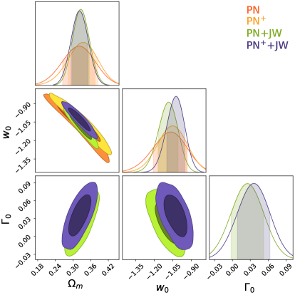
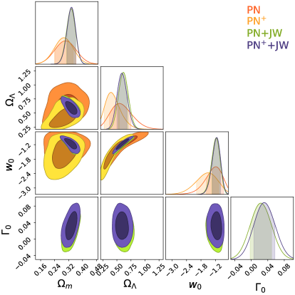
Figure 3: 1-2$\sigma$ C.L results for the $w$CDM model using SNIa Pantheon–PN (orange color), SNIa Pantheon+–PN⁺ (orange color), SNIa Pantheon & JW mock data – PN+JW (green color) and SNIa Pantheon+ & JW mock data – PN⁺+JW (purple color) baselines: Left: Flat case. Right: Non-flat case.

Additionally, $\Gamma_{0}$ is constrained with a value of $\Gamma_{0}=0.036^{+0.020}_{-0.022}$ mag using Pantheon+ and JW for the flat model. This means that there is not a significant deviation from the cosmological fits for the $w$CDM model using the JW mock sample compared to the observed SN samples.

4.3 Chevallier–Polarski–Linder (CPL) model

The constraints for this model are given in Figure 4. It is interesting to note that systematics improve for this model using Pantheon+ in comparison to the previous SN catalog, Pantheon. This is expected due to the density of data points at lower redshifts, where the CPL model can be well-constrained. For the flat model and using Pantheon data, we recover the $\Lambda$CDM model with $w_{0}=-1.111^{+0.110}_{-0.124}$ and $w_{a}=-1.252^{+1.354}_{-1.709}$ both at $1\sigma$. Something similar happened when we included the JW sample. This trend is confirmed when using Pantheon+ data, e.g. using Pantheon+ and JW results with $\Omega_{m}=0.323^{+0.022}_{-0.023}$, $w_{0}=-1.035^{+0.047}_{-0.056}$ and $w_{a}=0.130^{+0.432}_{-0.37}$. However, in the non-flat model, the estimations change when using solely SN measurements. The curvature estimation is deviated more than $1\sigma$ as for Pantheon $\Omega_{k}=0.31^{+0.22}_{-0.13}$, and for Pantheon+ $\Omega_{k}=0.447^{+0.14}_{-0.19}$. These results also deviate from the $\Lambda$CDM confirmation as both $w_{0}$ and $w_{a}$ do not recover the basic equations with $w_{0}=-1$ and $w_{a}=0$.

In this model, all the results for $\Gamma_{0}$ constraints are lower than the simulated 0.15 mag error, and therefore, we do not expect to have any systematic effects on the cosmological parameters contaminated by the simulated magnitude in the JW. The larger estimation, in comparison to previous models, was found using the Pantheon+ sample for which $\Gamma_{0}=0.039\pm 0.022$ mag.

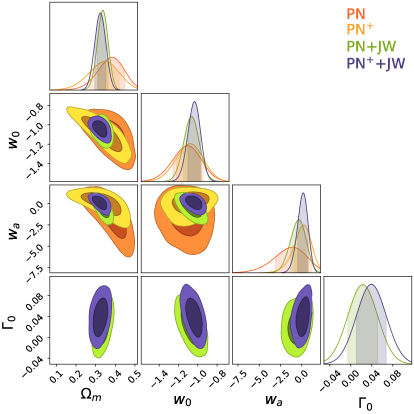
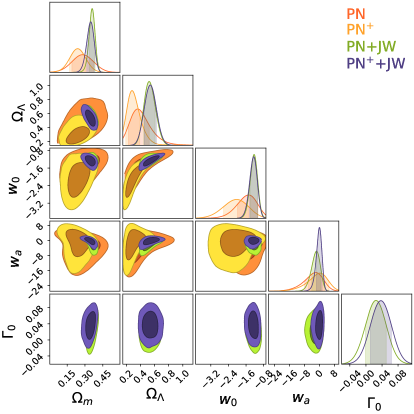
Figure 4: 1-2$\sigma$ C.L results for the CPL model using SNIa Pantheon–PN (orange color), SNIa Pantheon+–PN⁺ (yellow color), SNIa Pantheon & JW mock data – PN+JW (green color) and SNIa Pantheon+ & JW mock data – PN⁺+JW (purple color) baselines: Left: Flat case. Right: Non-flat case.

4.4 Jassal–Bagla–Padmanabhan (JBP) model

The constraints for this model are given in Figure 5. As we can notice, the flat version of this model recovers the correlation between the $\Omega_{m}$ and the $w_{0}$ parameters for all the datasets while the $w_{a}$ determination is done with a large error determination. Confirmation of $\Lambda$CDM occurs for Pantheon and JW combinations as $w_{0}=-1$ and $w_{a}=0$, while this not happen using Pantheon+, which results in a clear deviation as $w_{a}=1.403^{+0.650}_{-0.845}$. It is worth mentioning that the only negative $w_{a}$ value is obtained using the Pantheon dataset as $w_{a}=-0.721^{+1.787}_{-2.492}$. Using Pantheon, Pantheon+ and the Pantheon and JW combination has a parameter $w_{a}$ determination error larger than the average. For the fractional matter density, with Pantheon data, we obtain a larger estimation than Pantheon+, with $\Omega_{m}>0.3$ for Pantheon, and $\Omega_{m}<0.3$ for the Pantheon+ and the combination with JW.

For the non-flat model, we obtain different results, as none of the combinations return a deviation from the flat model. With Pantheon+ data we obtain $\Omega_{k}=0.48^{+0.20}_{-0.10}$, while the JW mock data brings the estimation closer to $\Omega_{k}=0$ without reaching flatness. It is worth noticing that Pantheon combinations result in negative $w_{a}$ values, while Pantheon+ combinations are opposite at $1\sigma$ with a large uncertainty.

Using the JBP model the larger $\Gamma_{0}$ determination is obtained using the Pantheon+ and JW for the non-flat version as $\Gamma_{0}=0.040\pm 0.022$ mag, which again discards the systematic error in the magnitude determination for the JW mock data.

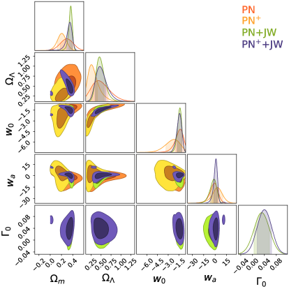
Figure 5: 1-2$\sigma$ C.L results for the JBP model using SNIa Pantheon–PN (orange color), SNIa Pantheon+–PN⁺ (yellow color), SNIa Pantheon & JW mock data – PN+JW (green color) and SNIa Pantheon+ & JW mock data – PN⁺+JW (purple color) baselines: Left: Flat case. Right: Non-flat case.

4.5 Exponential model

The constraints for this model are given in Figure 6. As we can notice, a correlation is presented in the parameter space between $w_{0}$ and $\Omega_{m}$ for all dataset combinations. For the flat model, all the combinations result in $w_{0}\sim-1$ between $1\sigma$ with a $\Omega_{m}\sim 0.3$. For the non-flat version is worth noticing that all the combinations using Pantheon data result in curvature estimations close to the ones expected for a flat universe. Being closer to flatness only with Pantheon data. Using the Pantheon+ dataset alone results in a larger deviation from the flatness as $\Omega_{k}=0.35^{+0.23}_{-0.11}$. This can be alleviated using the JW mock data as $\Omega_{k}=0.135^{+0.095}_{-0.072}$ reports a larger deviation than $1\sigma$ but near to the range of the expected value for a flat universe. Similar to the flat model, the fractional matter density value is close to $\Omega_{m}\sim 0.3$, being the lowest one obtained with Pantheon+ with $\Omega_{m}=0.262\pm 0.055$. In the case of $w_{0}$ the results are slightly lower than $w_{0}=-1$, being the same Pantheon+ the lower estimation as $w_{0}=-1.86^{+0.74}_{-0.48}$.

Using the Exponential model results for the determination of $\Gamma_{0}=0.036\pm 0.021$ in combination with Pantheon+ and JW means that the determination of the cosmological parameters in this model is not affected by the systematics in the JW mock data.

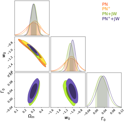
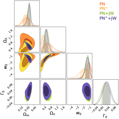
Figure 6: 1-2$\sigma$ C.L results for the exponential model using SNIa Pantheon–PN (orange color), SNIa Pantheon+–PN⁺ (yellow color), SNIa Pantheon & JW mock data – PN+JW (blue color) and SNIa Pantheon+ & JW mock data – PN⁺+JW (purple color) baselines: Left: Flat case. Right: Non-flat case.

4.6 Barboza–Alcaniz (BA) model

The constraints for this model are given in Figure 7. As we can notice for the flat model the lower value for $\Omega_{m}$ is the one obtained with the Pantheon+ and JW combination resulting in $\Omega_{m}=0.280^{+0.047}_{-0.081}$. Regarding the values of $w_{0}$ and $w_{a}$ for the flat models, all the combination results are consistent at $1\sigma$ with the $\Lambda$CDM model, as all the results fall in the range of $w_{0}\sim-1$ and $w_{a}=0$. Nevertheless, it is interesting to notice that the only negative value for $w_{a}$ is the one obtained using the Pantheon compilation with $w_{a}=0.723^{+1.047}_{-1.531}$. In general, this model agrees with a flat $\Lambda$CDM at $1\sigma$.

Meanwhile, the non-flat model shows larger deviations from the $\Lambda$CDM model as the curvature estimation is separated from the flatness in more than $1\sigma$ for all the combinations, except the Pantheon compilation as $\Omega_{k}=0.20^{+0.29}_{-0.24}$. Other results prefer $\Omega_{k}>0$.

In this model, the larger $\Gamma_{0}$ estimation is obtained for the non-flat model with the Pantheon+ and JW mock data combination as $\Gamma_{0}=0.039\pm 0.021$ mag, resulting similar to the previous models where the cosmological parameter inference is not affected by the error in magnitude for the simulated dataset.

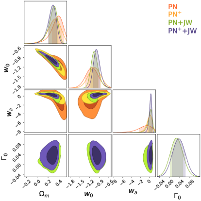
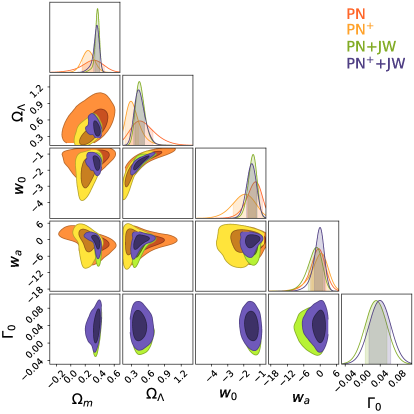
Figure 7: 1-2$\sigma$ C.L results for the BA model using SNIa Pantheon–PN (orange color), SNIa Pantheon+–PN⁺ (yellow color), SNIa Pantheon & JW mock data – PN+JW (green color) and SNIa Pantheon+ & JW mock data – PN⁺+JW (purple color) baselines: Left: Flat case. Right: Non-flat case.

5 Conclusions

In this paper, we studied new cosmological constraints in spatial curvature dark energy models. We extend the distance ladder method through an SNIa sample using the capabilities of JWST to forecast SNIa up to $z\sim 6$, considering the information on the star formation rates at high $z$. Comparing the results shown in Tables 1 and 2, notice that flat $\Lambda$CDM, flat $w$CDM, and flat exponential are the only models in which the value of $\Omega_{m}$ obtained using the Pantheon sample is less than $\Omega_{m}$ for Pantheon+, i.e. $\Omega_{m,\text{PN}}<\Omega_{m,\text{PN}^{+}}$.

However, in our analysis when including the JW mock data, the flat $\Lambda$CDM, non-flat $\Lambda$CDM, non-flat $w$CDM, and non-flat exponential are the cosmological models in which $\Omega_{m}$ for the combination PN+JW is less than $\Omega_{m}$ for PN⁺+JW, i.e. $\Omega_{m,\text{PN+JW}}<\Omega_{m,\text{PN}^{+}+\text{JW}}$. Showing a lower value of this parameter when we have higher SN at $z<1$.

In regards to JW forecasting, all models have a $\Gamma_{0,\text{PN}^{+}+\text{JW}}>\Gamma_{0,\text{PN+JW}}$. More SN at $z<1$ (e.g. Pantheon+) seems to raise the value of this $\Gamma_{0}$ parameter associated with JWST. Therefore, according to our $\Delta\mu$ equation (see below Eq.(3.3)), it is statistically better to employ Pantheon with JW forecasting due that the vector uncertainty is lower in comparison to the one obtained with Pantheon+ catalog. However, notice that the JW sample has been calibrated with Pantheon, therefore $\Gamma_{0}$ shows a preference for this SN sample.

We have studied the possibility of non-zero curvature in standard dark energy models, as demonstrated in [9]. The addition of our JW forecasting leads to an improvement in the statistics associated with $\Omega_{m}$. It is expected that the JWST will observe more luminous structures with a well-treated morphology, which can help us find more robust statistics in dark energy cosmologies.

Model (flat)	Dataset	$\Omega_{M}$	$w_{0}$	$w_{a}$	$\Gamma_{0}$
	PN	$0.290\pm 0.008$
	PN+JW	$0.295\pm 0.007$			$0.005^{+0.018}_{-0.018}$
$\Lambda$CDM	PN+	$0.311^{+0.010}_{-0.009}$
	PN++JW	$0.312\pm 0.008$			$0.028\pm 0.018$
	PN	$0.320^{+0.040}_{-0.045}$	$-1.073^{+0.100}_{-0.113}$
	PN+JW	$0.327^{+0.023}_{-0.021}$	$-1.086^{+0.057}_{-0.065}$		$0.025\pm 0.021$
$w$CDM	PN+	$0.334^{+0.036}_{-0.041}$	$-1.053^{+0.091}_{-0.095}$
	PN++JW	$0.322^{+0.023}_{-0.022}$	$-1.025^{+0.052}_{-0.062}$		$0.036^{+0.020}_{-0.022}$
	PN	$0.380^{+0.046}_{-0.058}$	$-1.111^{+0.110}_{-0.124}$	$-1.252^{+1.354}_{-1.709}$
	PN+JW	$0.336^{+0.021}_{-0.022}$	$-1.065^{+0.061}_{-0.064}$	$-0.399^{+0.668}_{-0.798}$	$0.022^{+0.023}_{-0.022}$
CPL	PN+	$0.343^{+0.054}_{-0.065}$	$-1.081^{+0.103}_{-0.118}$	$0.150^{+0.638}_{-0.936}$
	PN++JW	$0.323^{+0.022}_{-0.023}$	$-1.035^{+0.047}_{-0.056}$	$0.130^{+0.432}_{-0.537}$	$0.039\pm 0.022$
	PN	$0.358^{+0.064}_{-0.091}$	$-1.088^{+0.140}_{-0.162}$	$-0.721^{+1.787}_{-2.492}$
	PN+JW	$0.310^{+0.036}_{-0.048}$	$-1.106^{+0.075}_{-0.079}$	$0.873^{+1.216}_{-1.491}$	$0.029^{+0.023}_{-0.022}$
JBP	PN+	$0.268^{+0.095}_{-0.121}$	$-1.013^{+0.142}_{-0.153}$	$1.182^{+0.707}_{-1.073}$
	PN++JW	$0.280^{+0.039}_{-0.051}$	$-1.045^{+0.062}_{-0.063}$	$1.403^{+0.650}_{-0.845}$	$0.038^{+0.022}_{-0.021}$
	PN	$0.304^{+0.060}_{-0.066}$	$-1.044^{+0.128}_{-0.163}$
	PN+JW	$0.312^{+0.026}_{-0.025}$	$-1.062^{+0.060}_{-0.073}$		$0.025^{+0.022}_{-0.020}$
Exp	PN+	$0.321^{+0.050}_{-0.058}$	$-1.034^{+0.118}_{-0.129}$
	PN++JW	$0.306^{+0.026}_{-0.025}$	$-1.001^{+0.058}_{-0.063}$		$0.035^{+0.021}_{-0.023}$
	PN	$0.383^{+0.061}_{-0.111}$	$-1.124\pm 0.159$	$-0.723^{+1.047}_{-1.531}$
	PN+JW	$0.301^{+0.049}_{-0.092}$	$-1.045^{+0.109}_{-0.083}$	$0.301^{+0.254}_{-0.595}$	$0.028\pm 0.022$
BA	PN+	$0.323^{+0.076}_{-0.110}$	$-1.044^{+0.162}_{-0.156}$	$0.158^{+0.334}_{-0.614}$
	PN++JW	$0.280^{+0.047}_{-0.081}$	$-0.980^{+0.099}_{-0.075}$	$0.343^{+0.164}_{-0.311}$	$0.037\pm 0.021$

Table 1: Best-fit cosmological parameters at $1\sigma$ for the six flat models obtained by combining the following catalogs: Pantheon (PN) and Pantheon+ (PN⁺) with the JW simulated sample (JW). Empty cells denote parameters not defined in the model.

Model (non-flat)	Dataset	$\Omega_{M}$	$\Omega_{\Lambda}$	$w_{0}$	$w_{a}$	$\Gamma_{0}$	$\Omega_{k}$
	PN	$0.332\pm 0.043$	$0.761\pm 0.049$				$-0.092\pm 0.091$
	PN+JW	$0.306\pm 0.010$	$0.725\pm 0.017$			$0.018\pm 0.019$	$-0.031\pm 0.022$
$\Lambda$CDM	PN+	$0.328\pm 0.037$	$0.710\pm 0.041$				$-0.038\pm 0.076$
	PN++JW	$0.312\pm 0.010$	$0.695\pm 0.017$			$0.027\pm 0.019$	$-0.008\pm 0.023$
	PN	$0.302\pm 0.051$	$0.59^{+0.11}_{-0.20}$	$-1.29^{+0.38}_{-0.18}$			$0.11^{+0.21}_{-0.16}$
	PN+JW	$0.333^{+0.022}_{-0.019}$	$0.619^{+0.066}_{-0.073}$	$-1.19^{+0.16}_{-0.11}$		$0.023\pm 0.021$	$0.048\pm 0.058$
$w$CDM	PN+	$0.292\pm 0.045$	$0.435^{+0.068}_{-0.15}$	$-1.58^{+0.46}_{-0.29}$			$0.27^{+0.17}_{-0.11}$
	PN++JW	$0.334^{+0.022}_{-0.018}$	$0.595^{+0.065}_{-0.079}$	$-1.158^{+0.124}_{-0.152}$		$0.032\pm 0.021$	$0.071\pm 0.061$
	PN	$0.280\pm 0.077$	$0.412^{+0.060}_{-0.16}$	$-1.537^{+0.346}_{-0.451}$	$-3.6^{+5.4}_{-2.9}$		$0.31^{+0.22}_{-0.13}$
	PN+JW	$0.358^{+0.022}_{-0.017}$	$0.533^{+0.054}_{-0.077}$	$-1.238^{+0.126}_{-0.143}$	$-2.0^{+2.4}_{-1.3}$	$0.025\pm 0.021$	$0.109^{+0.061}_{-0.055}$
CPL	PN+	$0.239\pm 0.059$	$0.314^{+0.038}_{-0.11}$	$-2.059^{+0.465}_{-0.520}$	$-1.6^{+5.7}_{-2.7}$		$0.447^{+0.14}_{-0.09}$
	PN++JW	$0.344^{+0.029}_{-0.020}$	$0.539^{+0.069}_{-0.070}$	$-1.17^{+0.16}_{-0.11}$	$-0.34^{+1.5}_{-0.71}$	$0.037\pm 0.021$	$0.116\pm 0.057$
	PN	$0.292\pm 0.097$	$0.50^{+0.12}_{-0.24}$	$-1.50^{+0.62}_{-0.21}$	$-2.1^{+4.8}_{-2.6}$		$0.21^{+0.29}_{-0.21}$
	PN+JW	$0.358^{+0.031}_{-0.016}$	$0.493^{+0.055}_{-0.12}$	$-1.372^{+0.225}_{-0.281}$	$-3.0^{+4.9}_{-2.1}$	$0.031\pm 0.022$	$0.149^{+0.092}_{-0.061}$
JBP	PN+	$0.204\pm 0.072$	$0.315^{+0.044}_{-0.15}$	$-2.320^{+0.781}_{-1.051}$	$2.1^{+6.7}_{-4.3}$		$0.48^{+0.20}_{-0.10}$
	PN++JW	$0.328^{+0.056}_{-0.012}$	$0.517^{+0.076}_{-0.16}$	$-1.424^{+0.277}_{-0.347}$	$0.5^{+2.4}_{-1.4}$	$0.040\pm 0.022$	$0.155^{+0.10}_{-0.088}$
	PN	$0.289\pm 0.068$	$0.67^{+0.16}_{-0.32}$	$-1.24^{+0.50}_{-0.18}$			$0.04^{+0.30}_{-0.24}$
	PN+JW	$0.335^{+0.035}_{-0.021}$	$0.573^{+0.08}_{-0.12}$	$-1.33^{+0.31}_{-0.19}$		$0.028\pm 0.022$	$0.092^{+0.086}_{-0.076}$
Exp	PN+	$0.262\pm 0.055$	$0.391^{+0.046}_{-0.18}$	$-1.86^{+0.74}_{-0.48}$			$0.35^{+0.23}_{-0.11}$
	PN++JW	$0.340^{+0.032}_{-0.018}$	$0.526^{+0.073}_{-0.12}$	$-1.38^{+0.34}_{-0.22}$		$0.036\pm 0.021$	$0.134^{+0.095}_{-0.072}$
	PN	$0.287^{+0.15}_{-0.086}$	$0.52^{+0.11}_{-0.23}$	$-1.328^{+0.324}_{-0.459}$	$-1.1^{+2.6}_{-1.7}$		$0.20^{+0.29}_{-0.24}$
	PN+JW	$0.363^{+0.029}_{-0.014}$	$0.465^{+0.044}_{-0.090}$	$-1.447^{+0.206}_{-0.255}$	$-2.2^{+2.9}_{-1.3}$	$0.031\pm 0.022$	$0.172^{+0.075}_{-0.054}$
BA	PN+	$0.240\pm 0.069$	$0.332^{+0.046}_{-0.13}$	$-1.990^{+0.556}_{-0.658}$	$-0.7^{+3.2}_{-1.3}$		$0.43^{+0.19}_{-0.10}$
	PN++JW	$0.347^{+0.042}_{-0.012}$	$0.453^{+0.053}_{-0.10}$	$-1.522^{+0.254}_{-0.280}$	$-0.69^{+1.8}_{-0.92}$	$0.039\pm 0.021$	$0.200^{+0.081}_{-0.070}$

Table 2: Best-fit cosmological parameters at $1\sigma$ for the six non-flat cosmological models obtained for the following catalogs: combining Pantheon (PN) and Pantheon+ (PN⁺) datasets with the JW simulated sample (JW). Empty cells denote parameters not defined in the model..

Appendix A SNIa JWST baseline forecasting: data and priors

The simulated data set used is derived from the FLARE project, which has the goal of searching supernovas from population III at redshift $z\geq 10$ [77] by using the characteristics of the JWST in an area of 0.05 square degrees. Furthermore, the project employs four broadband in the NIRCAM filters (F150W, F200W, F322W2, F444W) with exposure times that can reach 10$\sigma$ limiting magnitudes of $m\gtrsim 27$ in these filters [9]. By using Monte Carlo methods it was found that for a specific project of JWST observation, at least 200 SNe Ia could be observed. Therefore, the mock sample is constructed using a flat $\Lambda$CDM model with $H_{0}=71.66$ km s^-1 Mpc^-1 and $\Omega_{m}=0.3$, as derived using Pantheon data [8]. To ensure consistency between the local and distant samples, we consider a Gaussian error associated with the supernovae distance modules of 0.15 mag and extrapolated them to a larger uncertainty with higher redshift, although this is an oversimplification of the typical distance measurements [80]. For the FLARE project [78] the simulations were done using the standard cosmology and a different SFR according to the redshift in which the simulation is done. Also, it is considered the calculation of the rate of occurrence to estimate the range of the detection needed in the telescope to perform the observations.

The used SFR functions are explicitly proposed to have a redshift dependence. For low $z\lesssim 3$, the function used is [81]:

$$\mathrm{SFR}(z)=K\frac{(a+bz)h}{1+(z/c)^{d}},$$ (A.1)

where $h=H_{0}/(100\mathrm{km}\mathrm{s}^{-1}\mathrm{Mpc}^{-1})$, $a=0.017$, $b=0.13$, $c=3.3$, and $d=5.3$. These quantities constrain $K$ with the SN rates observed. For higher redshifts between $3<z\leq 8$, the function used is:

$$\mathrm{SFR}(z)\propto(1+z)^{-3.6},$$ (A.2)

and for $z>8$:

$$\mathrm{SFR}(z)\propto(1+z)^{-10.4}.$$ (A.3)

Additionally, other SFRs are proposed for the whole interval [82]:

$$\mathrm{SFR}(z)=0.015\frac{(1+z)^{2.7}}{1+[(1+z)/2.9]^{5.6}},$$ (A.4)

or [83]:

$$\mathrm{SFR}(z)=\frac{C}{10^{A(z-z_{0})}+10^{B(z-z_{0})}},$$ (A.5)

using the constants $C=0.18$, $A=-0.997$, $B=0.241$, and $z_{0}=1.243$. All the parameterisations studied in Sec.2 for the SFR give similar redshift dependence with a peak in star formation in $z\sim 2$. The volume rate was calculated using the observed SN rate per redshift bin as [78]:

$$\dot{N}_{\mathrm{SN}}(z)=\frac{\dot{n}_{\mathrm{SLSN}}(z)}{1+z}\derivative{V}{z},$$ (A.6)

where the comoving volume can be rewritten as:

$$\dot{n}_{\mathrm{SLSN}}(z)=\varepsilon(z)\mathrm{SFR}(z),$$ (A.7)

where explicitly is expressed the comoving rate of SNe. $\varepsilon(z)$ is a factor of the efficiency taking into account the metallicity dependence. Even though, $\varepsilon(z)$ can be studied through GRBs [78]. So, the expected number of SN can be calculated as:

$$N_{\mathrm{SN}}=\Omega T\int_{z}^{z+\Delta z}\frac{\dot{n}_{\mathrm{SLSN}}(z)}{1+z}\derivative{V}{z}\mathrm{d}z,$$ (A.8)

resulting in a number per unit of redshift interval in the survey area. $\Omega$ is the survey area and $T$ is the dedicated time of observation. The redshift dependence also has to consider the number of SNIa progenitors that occur (as SNIa needs a White Dwarf) and the delay for the stellar evolution in such binary systems.

For the simulations of mock data sets the code developed by [84] is used to create light curves at different redshifts taking into account the calculated rate and detection of the observatory [78]. So, for the simulation the redshift $z$, the luminosity distance $D_{L}$, maximum light moment $t_{\mathrm{max}}$, V absolute magnitude $M_{\mathrm{V}}$, stretch and color are calculated for every SN. It is important to mention that the assumptions of the FLARE project imply that the JSWT will take deep observations for at least three years with a 90-day cadence allowing us to discover between 5 and 20 supernovae events meaning at least fifty in redshift $1<z<4$ [9]. Additionally, the simulation takes into account that the SNIa ideal observation time has to be from 2 weeks before the maximum up to one month after in which spectrum would have the ideal quality [85]. So, for the simulations, the results are the Hubble diagram for the apparent magnitude assuming detection with the NIRCam of the telescope.

References

- [1] Supernova Cosmology Project collaboration, Measurements of and from 42 high redshift supernovae, Astrophys. J. 517 (1999) 565 [astro-ph/9812133].
- [2] Supernova Search Team collaboration, Observational evidence from supernovae for an accelerating universe and a cosmological constant, Astron. J. 116 (1998) 1009 [astro-ph/9805201].
- [3] Boomerang collaboration, Cosmology from MAXIMA-1, BOOMERANG and COBE / DMR CMB observations, Phys. Rev. Lett. 86 (2001) 3475 [astro-ph/0007333].
- [4] SDSS collaboration, Detection of the Baryon Acoustic Peak in the Large-Scale Correlation Function of SDSS Luminous Red Galaxies, Astrophys. J. 633 (2005) 560 [astro-ph/0501171].
- [5] BOSS collaboration, The clustering of galaxies in the SDSS-III Baryon Oscillation Spectroscopic Survey: baryon acoustic oscillations in the Data Releases 10 and 11 Galaxy samples, Mon. Not. Roy. Astron. Soc. 441 (2014) 24 [1312.4877].
- [6] DES collaboration, Dark Energy Survey year 1 results: Cosmological constraints from galaxy clustering and weak lensing, Phys. Rev. D 98 (2018) 043526 [1708.01530].
- [7] D. Brout et al., The Pantheon+ Analysis: Cosmological Constraints, Astrophys. J. 938 (2022) 110 [2202.04077].
- [8] D. Scolnic et al., The Next Generation of Cosmological Measurements with Type Ia Supernovae, 1903.05128.
- [9] J. Lu, L. Wang, X. Chen, D. Rubin, S. Perlmutter, D. Baade et al., Constraints on Cosmological Parameters with a Sample of Type Ia Supernovae from JWST, Astrophys. J. 941 (2022) 71 [2210.00746].
- [10] C. Escamilla-Rivera and S. Capozziello, Unveiling cosmography from the dark energy equation of state, Int. J. Mod. Phys. D 28 (2019) 1950154 [1905.04602].
- [11] C. Escamilla-Rivera, Status on bidimensional dark energy parameterizations using SNe Ia JLA and BAO datasets, Galaxies 4 (2016) 8 [1605.02702].
- [12] L.A. Escamilla, W. Giarè, E. Di Valentino, R.C. Nunes and S. Vagnozzi, The state of the dark energy equation of state circa 2023, 2307.14802.
- [13] C. Escamilla-Rivera and A. Nájera, Dynamical dark energy models in the light of gravitational-wave transient catalogues, JCAP 03 (2022) 060 [2103.02097].
- [14] C. Escamilla-Rivera, M.A.C. Quintero and S. Capozziello, A deep learning approach to cosmological dark energy models, JCAP 03 (2020) 008 [1910.02788].
- [15] H.-C. Zhang, Dynamical dark energy can amplify the expansion rate of the Universe, Phys. Rev. D 107 (2023) 103529 [2305.16586].
- [16] L.G. Jaime, M. Jaber and C. Escamilla-Rivera, New parametrized equation of state for dark energy surveys, Phys. Rev. D 98 (2018) 083530 [1804.04284].
- [17] T. Clifton, P.G. Ferreira, A. Padilla and C. Skordis, Modified Gravity and Cosmology, Phys. Rept. 513 (2012) 1 [1106.2476].
- [18] L. Amendola, R. Gannouji, D. Polarski and S. Tsujikawa, Conditions for the cosmological viability of f(R) dark energy models, Phys. Rev. D 75 (2007) 083504 [gr-qc/0612180].
- [19] S. Bahamonde, K.F. Dialektopoulos, C. Escamilla-Rivera, G. Farrugia, V. Gakis, M. Hendry et al., Teleparallel gravity: from theory to cosmology, Rept. Prog. Phys. 86 (2023) 026901 [2106.13793].
- [20] Y.-F. Cai, S. Capozziello, M. De Laurentis and E.N. Saridakis, f(T) teleparallel gravity and cosmology, Rept. Prog. Phys. 79 (2016) 106901 [1511.07586].
- [21] DES collaboration, The Dark Energy Survey: more than dark energy – an overview, Mon. Not. Roy. Astron. Soc. 460 (2016) 1270 [1601.00329].
- [22] DESI collaboration, The DESI Experiment Part I: Science,Targeting, and Survey Design, 1611.00036.
- [23] LSST Dark Energy Science collaboration, The LSST Dark Energy Science Collaboration (DESC) Science Requirements Document, 1809.01669.
- [24] L. Amendola et al., Cosmology and fundamental physics with the Euclid satellite, Living Rev. Rel. 21 (2018) 2 [1606.00180].
- [25] J.P. Gardner et al., The James Webb Space Telescope, Space Sci. Rev. 123 (2006) 485 [astro-ph/0606175].
- [26] Y. Asada, M. Sawicki, G. Desprez, R. Abraham, M. Bradač, G. Brammer et al., Jwst catches the assembly of a ultra-low-mass galaxy, arXiv preprint arXiv:2212.07540 (2022) .
- [27] I. Yoon, C.L. Carilli, S. Fujimoto, M. Castellano, E. Merlin, P. Santini et al., Alma observation of a galaxy candidate discovered with jwst, arXiv preprint arXiv:2210.08413 (2022) .
- [28] B.E. Robertson et al., Identification and properties of intense star-forming galaxies at redshifts z 10, Nature Astron. 7 (2023) 611 [2212.04480].
- [29] Y. Harikane, M. Ouchi, M. Oguri, Y. Ono, K. Nakajima, Y. Isobe et al., A comprehensive study of galaxies at z 9–16 found in the early jwst data: Ultraviolet luminosity functions and cosmic star formation history at the pre-reionization epoch, The Astrophysical Journal Supplement Series 265 (2023) 5.
- [30] K. Luhman, P. Tremblin, S. Birkmann, E. Manjavacas, J. Valenti, C.A. de Oliveira et al., Jwst/nirspec observations of the planetary mass companion twa 27b, The Astrophysical Journal Letters 949 (2023) L36.
- [31] J.L. Bean, Q. Xue, P.C. August, J. Lunine, M. Zhang, D. Thorngren et al., High atmospheric metal enrichment for a saturn-mass planet, Nature 618 (2023) 43.
- [32] T.P. Greene, T.J. Bell, E. Ducrot, A. Dyrek, P.-O. Lagage and J.J. Fortney, Thermal emission from the earth-sized exoplanet trappist-1 b using jwst, Nature 618 (2023) 39.
- [33] T.S.-Y. Lai, L. Armus, T. Diaz-Santos, K.L. Larson, A. Evans, M.A. Malkan et al., Goals-jwst: Tracing agn feedback on the star-forming ism in ngc 7469, arXiv preprint arXiv:2209.06741 (2022) .
- [34] E.W. Schwieterman, S.L. Olson, D. Pidhorodetska, C.T. Reinhard, A. Ganti, T.J. Fauchez et al., Evaluating the plausible range of n2o biosignatures on exo-earths: An integrated biogeochemical, photochemical, and spectral modeling approach, The Astrophysical Journal 937 (2022) 109.
- [35] S. Mukherjee, J.J. Fortney, N.E. Batalha, T. Karalidi, M.S. Marley, C. Visscher et al., Probing the extent of vertical mixing in brown dwarf atmospheres with disequilibrium chemistry, The Astrophysical Journal 938 (2022) 107.
- [36] M. Leung, E.W. Schwieterman, M.N. Parenteau and T.J. Fauchez, Alternative methylated biosignatures. i. methyl bromide, a capstone biosignature, The Astrophysical Journal 938 (2022) 6.
- [37] T. Mikal-Evans, Detecting the proposed ch4–co2 biosignature pair with the james webb space telescope: Trappist-1e and the effect of cloud/haze, Monthly Notices of the Royal Astronomical Society 510 (2022) 980.
- [38] P. Wang, B.-Y. Su, L. Zu, Y. Yang and L. Feng, Exploring the Dark Energy Equation of State with JWST, 2307.11374.
- [39] S.A. Adil, U. Mukhopadhyay, A.A. Sen and S. Vagnozzi, Dark energy in light of the early JWST observations: case for a negative cosmological constant?, 2307.12763.
- [40] A.G. Riess, G.S. Anand, W. Yuan, S. Casertano, A. Dolphin, L.M. Macri et al., Crowded No More: The Accuracy of the Hubble Constant Tested with High Resolution Observations of Cepheids by JWST, 2307.15806.
- [41] F. Cogato, M. Moresco, L. Amati and A. Cimatti, An analytical late-Universe approach to the weaving of modern cosmology, 2309.01375.
- [42] M.G. Dainotti, G. Bargiacchi, A.L. Lenart, S. Nagataki and S. Capozziello, Quasars: Standard Candles up to z = 7.5 with the Precision of Supernovae Ia, Astrophys. J. 950 (2023) 45 [2305.19668].
- [43] R. Sandoval-Orozco, C. Escamilla-Rivera, R. Briffa and J. Levi Said, cosmology in the regime of quasar observations, 2309.03675.
- [44] Pan-STARRS1 collaboration, The Complete Light-curve Sample of Spectroscopically Confirmed SNe Ia from Pan-STARRS1 and Cosmological Constraints from the Combined Pantheon Sample, Astrophys. J. 859 (2018) 101 [1710.00845].
- [45] N. Lovyagin, A. Raikov, V. Yershov and Y. Lovyagin, Cosmological Model Tests with JWST, Galaxies 10 (2022) 108 [2212.06575].
- [46] H. Atek, M. Shuntov, L.J. Furtak, J. Richard, J.-P. Kneib, G. Mahler et al., Revealing galaxy candidates out to z 16 with JWST observations of the lensing cluster SMACS0723, MNRAS 519 (2023) 1201 [2207.12338].
- [47] C. Jacobs, K. Glazebrook, A. Calabrò, T. Treu, T. Nannayakkara, T. Jones et al., Early Results from GLASS-JWST. XVIII. A First Morphological Atlas of the 1 ¡ z ¡ 5 Universe in the Rest-frame Optical, ApJ 948 (2023) L13 [2208.06516].
- [48] H. Yan, Z. Ma, C. Ling, C. Cheng and J.-S. Huang, First Batch of z 11-20 Candidate Objects Revealed by the James Webb Space Telescope Early Release Observations on SMACS 0723-73, ApJ 942 (2023) L9 [2207.11558].
- [49] M. Castellano, A. Fontana, T. Treu, P. Santini, E. Merlin, N. Leethochawalit et al., Early Results from GLASS-JWST. III. Galaxy Candidates at z 9-15, ApJ 938 (2022) L15 [2207.09436].
- [50] D. Schaerer, R. Marques-Chaves, L. Barrufet, P. Oesch, Y.I. Izotov, R. Naidu et al., First look with JWST spectroscopy: Resemblance among z 8 galaxies and local analogs, A&A 665 (2022) L4 [2207.10034].
- [51] M.A. Marshall, S. Wilkins, T. Di Matteo, W.J. Roper, A.P. Vijayan, Y. Ni et al., The impact of dust on the sizes of galaxies in the Epoch of Reionization, MNRAS 511 (2022) 5475 [2110.12075].
- [52] K.A. Suess, R. Bezanson, E.J. Nelson, D.J. Setton, S.H. Price, P. van Dokkum et al., Rest-frame Near-infrared Sizes of Galaxies at Cosmic Noon: Objects in JWST’s Mirror Are Smaller than They Appeared, ApJ 937 (2022) L33 [2207.10655].
- [53] F. Zwicky, On the Red Shift of Spectral Lines through Interstellar Space, Proc. Nat. Acad. Sci. 15 (1929) 773.
- [54] E. Di Valentino, O. Mena, S. Pan, L. Visinelli, W. Yang, A. Melchiorri et al., In the realm of the Hubble tension—a review of solutions, Class. Quant. Grav. 38 (2021) 153001 [2103.01183].
- [55] E. Abdalla et al., Cosmology intertwined: A review of the particle physics, astrophysics, and cosmology associated with the cosmological tensions and anomalies, JHEAp 34 (2022) 49 [2203.06142].
- [56] L. Amendola and S. Tsujikawa, Dark Energy: Theory and Observations, Cambridge University Press (2010), 10.1017/CBO9780511750823.
- [57] P.D. Bari, Cosmology and the Early Universe, Taylor & Francis (2018).
- [58] G. Bargiacchi, M. Benetti, S. Capozziello, E. Lusso, G. Risaliti and M. Signorini, Quasar cosmology: dark energy evolution and spatial curvature, Mon. Not. Roy. Astron. Soc. 515 (2022) 1795 [2111.02420].
- [59] Planck collaboration, Planck 2018 results. VI. Cosmological parameters, Astron. Astrophys. 641 (2020) A6 [1807.06209].
- [60] M. Moresco, Addressing the Hubble tension with cosmic chronometers, 2307.09501.
- [61] X. Zheng, S. Cao, M. Biesiada, X. Li, T. Liu and Y. Liu, Multiple measurements of quasars acting as standard probes: model independent calibration and exploring the Dark Energy Equation of States, Sci. China Phys. Mech. Astron. 64 (2021) 259511 [2103.07139].
- [62] M. Chevallier and D. Polarski, Accelerating universes with scaling dark matter, Int. J. Mod. Phys. D 10 (2001) 213 [gr-qc/0009008].
- [63] E.V. Linder, Exploring the expansion history of the universe, Phys. Rev. Lett. 90 (2003) 091301 [astro-ph/0208512].
- [64] B.R. Dinda, H. Singirikonda and S. Majumdar, Constraints on cosmic curvature from cosmic chronometer and quasar observations, 2303.15401.
- [65] H.K. Jassal, J.S. Bagla and T. Padmanabhan, WMAP constraints on low redshift evolution of dark energy, Mon. Not. Roy. Astron. Soc. 356 (2005) L11 [astro-ph/0404378].
- [66] D. Staicova, DE Models with Combined H0 · rd from BAO and CMB Dataset and Friends, Universe 8 (2022) 631 [2211.08139].
- [67] W. Yang, S. Pan, E. Di Valentino, E.N. Saridakis and S. Chakraborty, Observational constraints on one-parameter dynamical dark-energy parametrizations and the tension, Phys. Rev. D 99 (2019) 043543 [1810.05141].
- [68] M.N. Castillo-Santos, A. Hernández-Almada, M.A. García-Aspeitia and J. Magaña, An exponential equation of state of dark energy in the light of 2018 CMB Planck data, Phys. Dark Univ. 40 (2023) 101225 [2212.01974].
- [69] E.M. Barboza, Jr. and J.S. Alcaniz, A parametric model for dark energy, Phys. Lett. B 666 (2008) 415 [0805.1713].
- [70] D. Brout, M. Sako, D. Scolnic, R. Kessler, C.B. D’Andrea, T.M. Davis et al., First cosmology results using type ia supernovae from the dark energy survey: Photometric pipeline and light-curve data release, The Astrophysical Journal 874 (2019) 106.
- [71] A.G. Riess et al., A Comprehensive Measurement of the Local Value of the Hubble Constant with 1 km /s /Mpc Uncertainty from the Hubble Space Telescope and the SH0ES Team, Astrophys. J. Lett. 934 (2022) L7 [2112.04510].
- [72] R.J. Foley et al., The Foundation Supernova Survey: Motivation, Design, Implementation, and First Data Release, Mon. Not. Roy. Astron. Soc. 475 (2018) 193 [1711.02474].
- [73] P.J. Brown, A.A. Breeveld, S. Holland, P. Kuin and T. Pritchard, SOUSA: the Swift Optical/Ultraviolet Supernova Archive, Astrophys. Space Sci. 354 (2014) 89 [1407.3808].
- [74] M. Ganeshalingam, W. Li, A.V. Filippenko, C. Anderson, G. Foster, E.L. Gates et al., Results of the lick observatory supernova search follow-up photometry program: Bvri light curves of 165 type ia supernovae, The Astrophysical Journal Supplement Series 190 (2010) 418.
- [75] B.E. Stahl et al., Lick Observatory Supernova Search Follow-Up Program: Photometry Data Release of 93 Type Ia Supernovae, Mon. Not. Roy. Astron. Soc. 490 (2019) 3882 [1909.11140].
- [76] R. Briffa, C. Escamilla-Rivera, J. Said Levi, J. Mifsud and N.L. Pullicino, Impact of priors on late time cosmology, Eur. Phys. J. Plus 137 (2022) 532 [2108.03853].
- [77] L. Wang et al., A First Transients Survey with JWST: the FLARE project, 1710.07005.
- [78] E. Regos and J. Vinko, Detection and Classification of Supernovae Beyond z 2 Redshift with the James Webb Space Telescope, Astrophys. J. 874 (2019) 158 [1811.00891].
- [79] X. Chen, L. Hu and L. Wang, Constraining Type Ia Supernova Delay Time with Spatially Resolved Star Formation Histories, Astrophys. J. 922 (2021) 15 [2101.06242].
- [80] M.M. Phillips, The Absolute Magnitudes of Type IA Supernovae, .
- [81] A.M. Hopkins and J.F. Beacom, On the normalization of the cosmic star formation history, The Astrophysical Journal 651 (2006) 142.
- [82] P. Madau and M. Dickinson, Cosmic Star Formation History, Ann. Rev. Astron. Astrophys. 52 (2014) 415 [1403.0007].
- [83] P.S. Behroozi, R.H. Wechsler and C. Conroy, The average star formation histories of galaxies in dark matter halos from z= 0–8, The Astrophysical Journal 770 (2013) 57.
- [84] K. Barbary, T. Barclay, R. Biswas, M. Craig, U. Feindt, B. Friesen et al., “SNCosmo: Python library for supernova cosmology.” Astrophysics Source Code Library, record ascl:1611.017, Nov., 2016.
- [85] L. Hu, X. Chen and L. Wang, Spectroscopic Studies of Type Ia Supernovae Using LSTM Neural Networks, Astrophys. J. 930 (2022) 70 [2202.02498].