Compatibility of all noisy qubit observables

Abstract

It is a crucial feature of quantum mechanics that not all measurements are compatible with each other. However, if measurements suffer from noise they may lose their incompatibility. Here we determine the critical visibility such that all qubit observables, i.e. all positive operator-valued measures (POVMs), become compatible. In addition, we apply our methods to quantum steering and Bell nonlocality. We obtain a tight local hidden state model for two-qubit Werner states of visibility $1/2$. Interestingly, this proves that POVMs do not help to demonstrate quantum steering for this family of states. As an implication, this also provides a new bound on how much white noise the two-qubit singlet can tolerate before it does not violate any Bell inequality.

I Introduction

Quantum mechanics provides a remarkably accurate framework for predicting the outcomes of experiments and has led to the development of numerous technological advancements. Despite its successes, it presents us with puzzling and counterintuitive phenomena that challenge our classical notions of reality. One of the key aspects that set quantum mechanics apart from classical physics is the concept of measurement incompatibility. In classical physics, measuring one property of a system does not affect the measurement of another property. In quantum mechanics, however, the situation is radically different. The uncertainty principle, formulated by Werner Heisenberg, establishes a fundamental limit to the precision with which certain pairs of properties can be simultaneously known [1].

A simple and well-known example is the fact that we cannot simultaneously measure the spin of a particle in two orthogonal directions. It is known that incompatible measurements are at the core of many quantum information tasks. For example, they are necessary to violate Bell inequalities [2, 3] and necessary to provide an advantage in quantum communication [4, 5, 6] or state discrimination tasks [7, 8, 9] (see also the reviews [10, 11]).

However, measurement devices always suffer from imprecision. Therefore, an apparatus measures in practice only a noisy version of the observables. If the noise gets too large, these noisy observables can become compatible even though they are incompatible in the noiseless limit [12]. In that case, the statistics of both observables can be obtained as a coarse-graining of just a single measurement and the two observables become jointly measurable. However, a detector that only measures compatible observables has limited power. Most importantly, it cannot be used for many quantum information processing tasks like demonstrating Bell-nonlocality since these require incompatible measurements. It is therefore important to ask, how much noise can be tolerated before all observables become jointly measurable.

Figure 1: A measurement device can perform different measurements (labeled with $a$) that produce an outcome $i$. If the measurements are too noisy they can be simulated by a device that just performs a single measurement. In this work, we address the question of how much noise can be tolerated before all qubit observables become jointly measurable.

In this work, we show that all qubit observables become jointly measurable at a critical visibility of $1/2$. This result has direct implications for related fields of quantum information, in particular, Bell nonlocality [13, 14] and quantum steering [15, 16, 17, 18, 19, 20]. More precisely, we use the connection between joint measurability and quantum steering [21, 22, 23] to show that the two-qubit Werner state [24]

$$\rho^{\eta}_{W}=\eta\ \outerproduct{\Psi^{-}}{\Psi^{-}}+(1-\eta)\ \mathds{1}/4$$ (1)

cannot demonstrate EPR-steering if $\eta\leq 1/2$. Here, $\ket{\Psi^{-}}=\frac{1}{\sqrt{2}}(\ket{01}-\ket{10})$ denotes the two-qubit singlet state. As an implication, we obtain that the same state does not violate any Bell inequality for arbitrary bipartite positive operator-valued measurements (POVM) applied to both sides whenever $\eta\leq 1/2$.

II Notation and joint measurability

Before we introduce the problem, we introduce the necessary notation. Qubit states are described by a positive semidefinite $2\times 2$ complex matrix $\rho\in\mathcal{L}(\mathbb{C}_{2})$, $\rho\geq 0$ with unit trace $\tr[\rho]=1$. They can be represented as $\rho=\left(\openone+\vec{x}\cdot\vec{\sigma}\right)/2$, where $\vec{x}\in\mathbb{R}^{3}$ is a three-dimensional real vector such that $|\vec{x}|\leq 1$, and $\vec{\sigma}=(\sigma_{X},\sigma_{Y},\sigma_{Z})$ are the standard Pauli matrices. In this notation, $\vec{x}$ is the corresponding Bloch vector of the qubit state. General qubit measurements are described by a positive operator-valued measure (POVM), which is a set of positive semidefinite ($A_{i|a}\geq 0$) operators $\{A_{i|a}\}_{i}$ that sum to the identity, $\sum_{i}A_{i|a}=\mathds{1}$. Here, we use the label $"a"$ to distinguish between different measurements, while $"i"$ denotes the outcome of a given POVM (see also Fig. 1). In quantum theory, the probability of outcome $i$ when performing the POVM with elements $A_{i|a}$ on the state $\rho$ is given by Born’s rule,

$$p(i|a,\rho)=\tr[A_{i|a}\ \rho]\,.$$ (2)

Because every qubit POVM can be written as a coarse-graining of rank-1 projectors [25], we may restrict ourselves to POVMs proportional to rank-1 projectors. (We could also restrict ourselves to POVMs with at most four outcomes [26] but this is not necessary in what follows.) Thus, we write Alice’s measurements as $A_{i|a}=p_{i}\outerproduct{\vec{a}_{i}}{\vec{a}_{i}}$, where $p_{i}\geq 0$ and $\outerproduct{\vec{a}_{i}}{\vec{a}_{i}}=\big{(}\mathds{1}+\vec{a}_{i}\cdot\vec{\sigma}\big{)}/2$ for some normalized vector $\vec{a}_{i}\in\mathbb{R}^{3}$ ($|\vec{a}_{i}|=1$). As a consequence of $\sum_{i}A_{i|a}=\mathds{1}$ we obtain $\sum_{i}p_{i}=2$ and $\sum_{i}p_{i}\ \vec{a}_{i}=\vec{0}$.

These expressions are valid if all measurements and states are perfectly implemented. However, noise is usually unavoidable in experiments and in a more realistic scenario, the correlations are damped by a certain factor $\eta$. In this sense, we define the noisy measurement as

$$A^{\eta}_{i|a}=\eta\ A_{i|a}+(1-\eta)\cdot\tr[A_{i|a}]\ \mathds{1}/2\,.$$ (3)

With the notation introduced above the POVM elements become $A^{\eta}_{i|a}=p_{i}\big{(}\mathds{1}+\eta\ \vec{a}_{i}\cdot\vec{\sigma}\big{)}/2$ (again with $\sum_{i}p_{i}=2$, $|\vec{a}_{i}|=1$ and $\sum_{i}p_{i}\ \vec{a}_{i}=\vec{0}$). The goal of this work is to determine the critical value of $\eta$ such that all qubit POVMs become jointly measurable, a concept we introduce now.

A set of measurements $\{A_{i|a}\}_{i,a}$ is jointly measurable if there exists a single measurement (so-called parent POVM) $\{G_{\lambda}\}_{\lambda}$ such that the statistics of all measurements in the set can be obtained by classical post-processing of the data of that single parent measurement. More precisely, if for every POVM in the set there exist conditional probabilities $p(i|a,\lambda)$ such that:

$$A_{i|a}=\sum_{\lambda}p(i|a,\lambda)\ G_{\lambda}\,.$$ (4)

If this is satisfied, all measurements in the set can be simulated by the single parent POVM with operators $G_{\lambda}$: First, the parent POVM is measured on the quantum state $\rho$ in which outcome $\lambda$ occurs with probability $p(\lambda|\rho)=\tr[G_{\lambda}\ \rho]$. Second, given the POVM "a" we want to simulate, the outcome $i$ is produced with probability $p(i|a,\lambda)$. In total, the probability of outcome $i$ becomes:

$$\sum_{\lambda}p(i|a,\lambda)p(\lambda|\rho)=\sum_{\lambda}p(i|a,\lambda)\tr[G_{\lambda}\ \rho]=\tr[A_{i|a}\ \rho]\,.$$ (5)

Here, we used the linearity of the trace. This perfectly simulates a given POVM with elements $\{A_{i|a}\}_{i}$, since this is the same expression as if the measurement was directly performed on the quantum state $\rho$ given by Eq. (2).

The most prominent example are the two noisy observables $A^{\eta}_{\pm|x}=(\mathds{1}\pm 1/\sqrt{2}\ \sigma_{x})/2$ and $A^{\eta}_{\pm|z}=(\mathds{1}\pm 1/\sqrt{2}\ \sigma_{z})/2$ where $\eta=1/\sqrt{2}$. We can consider the following measurement with four outcomes $\lambda=(i,j)$ where $i,j\in\{+1,-1\}$:

$$G_{(i,j)}=\frac{1}{4}\left(\mathds{1}+\frac{i}{\sqrt{2}}\sigma_{x}+\frac{j}{\sqrt{2}}\sigma_{z}\right)\,.$$ (6)

One can check that this is a valid POVM and that $A^{\eta}_{i|x}=\sum_{j}G_{(i,j)}$ as well as $A^{\eta}_{j|x}=\sum_{i}G_{(i,j)}$. Therefore, the statistics of both observables $\{A^{\eta}_{i|x}\}_{i}$ and $\{A^{\eta}_{j|z}\}_{j}$ can be obtained from the statistics of just a single measurement.

III Construction for general measurements

Now we consider not only two observables but the set of all noisy qubit observables $\{A^{\eta}_{i|a}\}_{i,a}$. We show that if $\eta\leq 1/2$ this set becomes jointly measurable and a single parent measurement can simulate the statistics of all of these observables.

III.1 The protocol

For the protocol, we define two functions. The first one is the sign function, which is defined as $\operatorname{sgn}{(x)}:=+1$ if $x\geq 0$ and $\operatorname{sgn}{(x)}:=-1$ if $x<0$. Similarly, the function $\Theta(x)$ is defined as $\Theta(x):=x$ if $x\geq 0$ and $\Theta(x):=0$ if $x<0$.

The parent POVM $\{G_{\vec{\lambda}}\}_{\vec{\lambda}}$ is the observable with elements

$$G_{\vec{\lambda}}=\frac{1}{4\pi}(\mathds{1}+\vec{\lambda}\cdot\vec{\sigma})\,.$$ (7)

Here, $\vec{\lambda}$ is a normalized vector uniformly distributed on the unit radius sphere $S_{2}$. Physically, this corresponds to a (sharp) projective measurement with outcome $\vec{\lambda}$, where the measurement direction is chosen randomly (according to the Haar measure) on the Bloch sphere.

For a given POVM with operators $A^{1/2}_{i|a}=p_{i}\big{(}\mathds{1}+1/2\ \vec{a}_{i}\cdot\vec{\sigma}\big{)}/2$ where $\sum_{i}p_{i}=2$, $|\vec{a}_{i}|=1$, and $\sum_{i}p_{i}\ \vec{a}_{i}=\vec{0}$, we define the following function that associates a real-valued number to each point in $\vec{x}\in\mathbb{R}^{3}$:

$$f:\mathbb{R}^{3}\to\mathbb{R}:\ f(\vec{x}):=\sum_{i}p_{i}\ \Theta(\vec{x}\cdot\vec{a}_{i})\,.$$ (8)

Now, we choose a coordinate frame $x,y,z$ in which $f(\vec{v}_{s_{x}s_{y}s_{z}})\leq 1$ for all $s_{x},s_{y},s_{z}\in\{+1,-1\}$, where the eight vectors $\vec{v}_{s_{x}s_{y}s_{z}}$ are defined as $\vec{v}_{s_{x}s_{y}s_{z}}:=(s_{x},s_{y},s_{z})^{T}$ (they form the vertices of a cube). We show below that one can always find such a frame.

After choosing the coordinate frame, we define the conditional probabilities as:

$$p(i|a,\vec{\lambda})=p_{i}\cdot\Theta(\vec{a}_{i}\cdot\vec{v}_{s_{x}s_{y}s_{z}})+\frac{(1-f(\vec{v}_{s_{x}s_{y}s_{z}}))\alpha_{i}}{\sum_{i}\alpha_{i}}\,.$$ (9)

Here, we denote $s_{k}:=\operatorname{sgn}{(\lambda_{k}})$ for $k\in\{x,y,z\}$, where $\vec{\lambda}=(\lambda_{x},\lambda_{y},\lambda_{z})$. In addition, $\alpha_{i}$ is defined as:

$$\alpha_{i}:=\frac{p_{i}}{2}\left(1-\frac{1}{4}\sum_{s_{x},s_{y},s_{z}=\pm 1}\Theta(\vec{a}_{i}\cdot\vec{v}_{s_{x}s_{y}s_{z}})\right)\,.$$ (10)

III.2 Idea of the protocol

Suppose for now that it is possible to find a suitable coordinate frame in which $f(\vec{v}_{s_{x}s_{y}s_{z}})\leq 1$ for all eight vectors. Since this part is more technical, we discuss it at the end of this section. We can check that the conditional probabilities are indeed well-defined. Namely, they are positive and sum to one. Positivity follows from the fact that $p_{i}\geq 0$ and $\Theta(x)\geq 0$ (for all $x\in\mathbb{R}$). In addition, $f(\vec{v}_{s_{x}s_{y}s_{z}})\leq 1$ and the prove that $\alpha_{i}\geq 0$ is given in Appendix A (see Lemma 1 (2)). A quick calculation also shows that the probabilities sum to one:

$$\sum_{i} p(i|a,\vec{\lambda})=f(\vec{v}_{s_{x}s_{y}s_{z}})+(1-f(\vec{v}_{s_{x}s_{y}s_{z}}))=1\,.$$ (11)

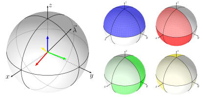
Figure 2: An illustration of the conditional probabilities $p(i|a,\vec{\lambda})$ for a SIC-POVM [27]: The different outcomes $i$ are represented with different colors and the colored vectors in the large sphere represent $p_{i}\cdot\vec{a}_{i}$. The opacity of the colors on the right side represents the probability to output $i$ given that $\vec{\lambda}$ lies in that region of the sphere, hence $p(i|a,\vec{\lambda})$. This function is constant in each octant of the sphere. For the $\vec{\lambda}$ shown here ($s_{x}=-1$, $s_{y}=s_{z}=+1$), the outcome is most likely blue ($50\%$) or green ($49\%$). (more details in Appendix D)

Now we are in a position to show that

$$A^{1/2}_{i|a}=\int_{S_{2}}\mathrm{d}\vec{\lambda}\ p(i|a,\vec{\lambda})\ G_{\vec{\lambda}}\,.$$ (12)

We give the detailed proof in Appendix C but sketch the main idea here. It is important to recognize that the function $p(i|a,\vec{\lambda})$ is constant in each octant of the chosen coordinate frame since it only depends on the signs of the components of $\vec{\lambda}$ (see Fig. 2 for an illustration). Intuitively speaking, this leads to a coarse-graining of the measurement outcomes $\vec{\lambda}$ in each octant. These coarse-grained observables $G_{s_{x}s_{y}s_{z}}$ behave like a noisy measurement in the direction of the corresponding vector $\vec{v}_{s_{x}s_{y}s_{z}}$. More precisely, we calculate in Appendix C.1 that:

$$G_{s_{x}s_{y}s_{z}}:= \int_{S_{2}|\operatorname{sgn}(\lambda_{k})=s_{k}}\mathrm{d}\vec{\lambda}\ G_{\vec{\lambda}}=\frac{\mathds{1}}{8}+\frac{\vec{v}_{s_{x}s_{y}s_{z}}\cdot\vec{\sigma}}{16}\,.$$ (13)

It turns out that the observable $A^{1/2}_{i|a}$ can be written as a mixture of these $G_{s_{x}s_{y}s_{z}}$ according to the following formula that we prove in Appendix C (Eq. (57)):

$$A^{1/2}_{i|a}= \sum_{s_{x},s_{y},s_{z}=\pm 1}p(i|a,\vec{\lambda})\ G_{s_{x}s_{y}s_{z}}$$ (14)

$$= \sum_{s_{x},s_{y},s_{z}=\pm 1}p_{i}\cdot\Theta(\vec{a}_{i}\cdot\vec{v}_{s_{x}s_{y}s_{z}})\ G_{s_{x}s_{y}s_{z}}+\alpha_{i}\mathds{1}\,.$$ (15)

To give an example, consider the blue vector in Fig. 2 for which $\vec{a}_{1}=(0,0,1)^{T}$ and $p_{1}=1/2$, hence $A^{1/2}_{1|a}=p_{1}\big{(}\mathds{1}+1/2\ \vec{a}_{1}\cdot\vec{\sigma}\big{)}/2=\mathds{1}/4+\sigma_{z}/8$. Direct calculation shows that $p_{1}\cdot\Theta(\vec{a}_{1}\cdot\vec{v}_{s_{x}s_{y}s_{z}})=1/2$ if $s_{z}=+1$ (and zero if $s_{z}=-1$) as well as $\alpha_{1}=0$. It is then easy to check that $1/2(G_{+++}+G_{+-+}+G_{-++}+G_{--+})=\mathds{1}/4+\sigma_{z}/8=A^{1/2}_{1|a}$ (see also Fig. 3).

The identity in Eq. (15) is the idea behind the protocol: to find a set of coarse-grained observables $G_{s_{x}s_{y}s_{z}}$ that can be used to decompose the observables $A^{1/2}_{i|a}$. The conditional probabilities $p(i|a,\vec{\lambda})$ are exactly constructed due to this expression. The first term in $p(i|a,\vec{\lambda})$, namely $p_{i}\cdot\Theta(\vec{v}_{s_{x}s_{y}s_{z}}\cdot\vec{a}_{i})$ is the coefficient that comes from the decomposition of $A^{1/2}_{i|a}$ in terms of $G_{s_{x}s_{y}s_{z}}$. The second term in $p(i|a,\vec{\lambda})$ is constructed to add the noise term $\alpha_{i}\mathds{1}$. When we evaluate the integral in Eq. (12) and use the definition of $G_{s_{x}s_{y}s_{z}}$, it reduces to that identity in Eq. (15). (Details in Appendix C)

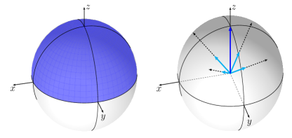
Figure 3: Whenever $\vec{\lambda}$ lies in one of the four octants in the upper hemisphere $\lambda_{z}\geq 1$ (or $s_{z}=+1$), the blue outcome is produced with probability $1/2$. Collecting all results $\vec{\lambda}$ from one octant behaves like the noisy observable $G_{s_{x}s_{y}s_{z}}$ represented with the cyan arrows in the right picture. The sum of these observables simulates the desired (blue) operator $A^{1/2}_{1|a}$. (In the right picture the arrows are twice as long for illustrative reasons.)

However, while the above identity holds in all coordinate frames, it can be translated into a protocol with well-defined probabilities only if $\sum_{i}p_{i}\cdot\Theta(\vec{v}_{s_{x}s_{y}s_{z}}\cdot\vec{a}_{i})=f(\vec{v}_{s_{x}s_{y}s_{z}})\leq 1$ for all $s_{x},s_{y},s_{z}\in\{+1,-1\}$. We can show now that such a coordinate frame always exists. The proof has two steps, the first step is a general bound on the sum of these eight functional values. Namely, in any coordinate frame, it turns out that:

$$\sum_{s_{x},s_{y},s_{z}=\pm 1}f(\vec{v}_{s_{x}s_{y}s_{z}})\leq 8\,.$$ (16)

The second part of the proof uses a theorem by Hausel, Makai, and Szűcs [28] (see Theorem 1 in that reference) that applies to continuous real-valued functions on $S_{2}$ that have the additional property that $f(\vec{x})=f(-\vec{x})$. We show in Appendix B that these conditions are indeed fulfilled. More precisely, they show that there always exists a cube inscribed to the two-sphere such that the eight functional values coincide at the vertices of that cube. Since the vectors $\vec{v}_{s_{x}s_{y}s_{z}}$ form precisely a cube, there exists a coordinate frame in which $f(\vec{v}_{s_{x}s_{y}s_{z}})=C$ for all $s_{x},s_{y},s_{z}\in\{+1,-1\}$. Combining this with the above bound in Eq. (16), we obtain $8C\leq 8$ and therefore $f(\vec{v}_{s_{x}s_{y}s_{z}})\leq 1$ in that specific coordinate frame. (see Appendix B for more details)

The theorem in Ref. [28] is a special case of a family of so-called Knaster-type theorems. They state that for a given continuous real-valued function on the sphere, a certain configuration of points can always be rotated such that the functional values coincide at each of these points. Other interesting related results concerning $S_{2}$ are due to Dyson [29], Livesay [30], or Floyd [31].

We want to remark that we do not necessarily have to choose a frame in which all of these eight values coincide. For the protocol, it is only necessary that all of these eight values are smaller than one, and every coordinate frame that satisfies this property can be chosen. Note that we do not give an explicit way to construct such a frame for all cases. However, in many cases, it turns out that an explicit coordinate frame can be found. In Appendix D, we show this for the case of POVMs with two or three outcomes. We also show that for the case of the four-outcome SIC-POVM [27], any coordinate frame can be chosen. See also Appendix D for further examples and more illustrations.

IV Local models for entangled quantum states

Now we apply the developed techniques to Bell nonlocality and quantum steering. Consider Alice and Bob share a two-qubit Werner state [24]:

$$\rho^{\eta}_{W}=\eta\outerproduct{\Psi^{-}}{\Psi^{-}}+(1-\eta)\ \mathds{1}/4$$ (17)

where $\ket{\Psi^{-}}=\frac{1}{\sqrt{2}}(\ket{01}-\ket{10})$ denotes the two-qubit singlet. Alice and Bob can apply arbitrary POVMs on their qubit. As before, we denote Alice’s measurement operators with $A_{i|a}=p_{i}\outerproduct{\vec{a}_{i}}{\vec{a}_{i}}=\big{(}\mathds{1}+\vec{a}_{i}\cdot\vec{\sigma}\big{)}/2$ (with $p_{i}\geq 0$, $|\vec{a}_{i}|=1$ and $\sum_{i}p_{i}=2$). Similarly, Bob can perform an arbitrary POVM with elements $B_{j|b}$ that are defined analogously. Note, that Alice’s and Bob’s measurements are now completely arbitrary, i.e. they are not noisy. Instead, the entangled state is not pure but has a certain amount of white noise.

The correlations when Alice and Bob apply local POVMs to this state become:

$$p(i,j|a,b)= \tr[(A_{i|a}\otimes B_{j|b})\ \rho^{\eta}_{W}]\,.$$ (18)

It is a fundamental question in Bell nonlocality, for which $\eta$ these correlations are local or violate a Bell inequality. It is known, that two-qubit Werner states violate the CHSH inequality [32] for $\eta>1/\sqrt{2}\approx 0.7071$. Vertesi showed that they violate another Bell inequality whenever $\eta>0.7056$ [33].

On the other hand, Werner showed in his seminal paper from 1989 that all of these states are local for bipartite projective measurements if $\eta\leq 1/2$ [24] albeit they are entangled if $\eta>1/3$. Later, this bound was improved by Acin, Toner, and Gisin, who showed that the state is local whenever $\eta\leq 1/K_{G}(3)$ [34]. Here, $K_{G}(3)$ is the so-called Grothendieck constant of order three and the best current bound is by Designolle et al. $1.4367\leq K_{G}(3)\leq 1.4546$ [35]. This implies that $\rho^{\eta}_{W}$ is local if $\eta\leq 0.6875$ and violates a Bell inequality if $\eta\leq 0.6961$. However, these local models only apply to projective measurements.

Considering all POVMs, Barrett found a local model for all POVMs whenever $\eta\leq 5/12$ [25]. Using a technique developed in Ref. [36, 37], the best bound is again by Ref. [35] which shows that $\rho^{\eta}_{W}$ is local for all observables if $\eta\leq 0.4583$. Based on the connections made in Ref. [21, 22, 23], we can now show that whenever $\eta\leq 1/2$ we cannot violate any Bell inequality since all correlations can be described by the following local model:

1. Bob’s system is in a well-defined pure qubit state $\rho_{\vec{\lambda}}={\big{(}\mathds{1}+\vec{\lambda}\cdot\vec{\sigma}\big{)}/2}$. Here, $\vec{\lambda}$ is uniformly and independently distributed on the unit radius sphere $S_{2}$.

2. Alice chooses her POVM with operators $A_{i|a}=p_{i}(\mathds{1}+\vec{a}_{i}\cdot\vec{\sigma})/2$. She flips all vectors $\vec{a}_{i}\mapsto-\vec{a}_{i}$ (to account for the anticorrelations in the singlet). Now, she applies precisely the same steps as in the previous protocol for the given values of $p_{i}$, vectors $\vec{a}_{i}$, and $\vec{\lambda}$. Namely, she chooses a suitable coordinate frame and produces her outcome $i$ according to the conditional probabilities $p(i|a,\vec{\lambda})$ in Eq. (9).

3. Bob chooses his POVM with elements $B_{j|b}$ and performs a quantum measurement on his state $\rho_{\vec{\lambda}}$.

The simplest way to see that this reproduces the desired correlations is to observe that the same calculations we did for the measurement operators before apply also to the states here. This is due to the duality of states and measurements in quantum mechanics. More precisely, the distribution of the state $\rho_{\vec{\lambda}}=\frac{1}{4\pi}\big{(}\mathds{1}+\vec{\lambda}\cdot\vec{\sigma}\big{)}/2$ is exactly the same expression as the one for the parent POVM in Eq. (7). The difference is only a factor of $2$ since states and measurements are normalized differently. Now, if we sum over all the states where Alice outputs $i$, Bob’s system behaves like the state

$$\rho_{B}(i)= \int_{S_{2}}\mathrm{d}\vec{\lambda}\ p(i|a,\vec{\lambda})\rho_{\vec{\lambda}}=p_{i}\big{(}\mathds{1}-\vec{a}_{i}\cdot\vec{\sigma}/2\big{)}/4\,.$$ (19)

It is important to notice that this is precisely the post-measurement state of Bob’s qubit when Alice performs the actual measurement $\{A_{i|a}\}_{i}$ on the Werner state with $\eta=1/2$ and obtains outcome $i$:

$$\rho_{B}(i)= \tr_{A}[(A_{i|a}\otimes\mathds{1})\rho^{1/2}_{W}]$$ (20)

$$= \frac{1}{2}p_{i}(\mathds{1}-\vec{a}_{i}\cdot\vec{\sigma})/4+\frac{1}{2}p_{i}\ \mathds{1}/4$$ (21)

$$= p_{i}\big{(}\mathds{1}-\vec{a}_{i}\cdot\vec{\sigma}/2\big{)}/4\,.$$ (22)

Intuitively speaking, there is no difference for Bob’s qubit if Alice performs the protocol above or performs the measurement on the actual Werner state for $\eta=1/2$. Therefore, when Bob applies his POVM, the resulting statistic becomes the same in both cases. Hence, the protocol above simulates the statistics of arbitrary local POVMs on the state $\rho^{1/2}_{W}$ in a local way.

This model is even a so-called local hidden state model which implies that the state $\rho^{1/2}_{W}$ is not steerable [15, 16, 19]. In the most fundamental steering scenario, we consider two parties, Alice and Bob, that share an entangled quantum state. The question is, whether Alice can steer Bob’s state by applying a measurement on her side. However, Bob wants to exclude the possibility that his system is prepared in a well-defined state that is known to Alice. Then, Alice could just use her knowledge of the "hidden state" to pretend to Bob that she can steer his state albeit in reality, they do not share any entangled quantum state at all. This is precisely the case in the above protocol, proving that the state $\rho^{\eta}_{W}$ cannot demonstrate quantum steering whenever $\eta\leq 1/2$. This was known before for the restricted case of projective measurements $A_{\pm|a}=(\mathds{1}\pm\vec{a}\cdot\sigma)/2$ [16]. When all observables are considered, the best model so far is due to Barrett [25], which was shown to be a local hidden state model by Quintino et al. [38]. That model shows that $\rho_{W}^{\eta}$ cannot demonstrate steering if $\eta\leq 5/12$. Numerical evidence suggested that the same holds for all $\eta\leq 1/2$ [39, 40, 41]. Our model shows, that this is indeed the case.

On the other hand, it is known that the two-qubit Werner state can demonstrate steering whenever $\eta>1/2$ [16]. Therefore, the bound of $\eta=1/2$ is tight. Due to the connection between steering and joint measureability [22, 21, 23], $\eta=1/2$ is also tight for the problem of joint measureability, ensuring the optimality of our above protocol.

.

V Conclusion

In this work, we provided tight bounds on how much noise a measurement device can tolerate before all qubit observables become jointly measurable. We considered the most general set of measurements (POVMs) and applied our techniques to quantum steering and Bell nonlocality. Exploiting the connection between joint measurability and steering [22, 21, 23], we found a tight local hidden state model for two-qubit Werner states of visibility $\eta=1/2$. This solves Problem 39 on the page of Open quantum problems [42] (see also Ref. [43]) and Conjecture 1 of Ref. [40]. An important direction for further research is the generalization to higher dimensional systems [44, 45].

Note: At the very last stage of this work, Zhang and Chitambar [46] uploaded a paper that proves the same result.

Appendix A A helpful lemma

Lemma 1.

Given the eight vectors $\vec{v}_{s_{x}s_{y}s_{z}}=(s_{x},s_{y},s_{z})^{T}$ where $s_{x},s_{y},s_{z}\in\{+1,-1\}$ (for example, $\vec{v}_{+--}=(+1,-1,-1)^{T}$) that form the vertices of a cube with side length 2 and an arbitrary vector $\vec{a}\in\mathbb{R}^{3}$. In addition, the function $\Theta(x)$ is defined as $\Theta(x):=x$ if $x\geq 0$ and $\Theta(x):=0$ if $x<0$ (equivalent: $\Theta(x):=(|x|+x)/2$ ). We prove the following properties:

$$(1)\, \sum_{s_{x},s_{y},s_{z}=\pm 1}|\vec{v}_{s_{x}s_{y}s_{z}}\cdot\vec{a}|\leq 8\cdot|\vec{a}|$$ (23)

$$(2)\, \sum_{s_{x},s_{y},s_{z}=\pm 1}\Theta(\vec{v}_{s_{x}s_{y}s_{z}}\cdot\vec{a})\leq 4\cdot|\vec{a}|$$ (24)

$$(3)\, \sum_{s_{x},s_{y},s_{z}=\pm 1}(\vec{v}_{s_{x}s_{y}s_{z}}\cdot\vec{a})\ \vec{v}_{s_{x}s_{y}s_{z}}=8\cdot\vec{a}$$ (25)

$$(4)\, \sum_{s_{x},s_{y},s_{z}=\pm 1}\Theta(\vec{v}_{s_{x}s_{y}s_{z}}\cdot\vec{a})\ \vec{v}_{s_{x}s_{y}s_{z}}=4\cdot\vec{a}$$ (26)

Proof.

(1) We apply the Cauchy-Schwarz inequality to the following two eight-dimensional vectors:

$$\begin{pmatrix}1\\ 1\\ \vdots\\ 1\end{pmatrix}\cdot\begin{pmatrix}|\vec{v}_{+++}\cdot\vec{a}|\\ |\vec{v}_{++-}\cdot\vec{a}|\\ \vdots\\ |\vec{v}_{---}\cdot\vec{a}|\end{pmatrix} \leq\absolutevalue{\begin{pmatrix}1\\ 1\\ \vdots\\ 1\end{pmatrix}}\cdot\absolutevalue{\begin{pmatrix}|\vec{v}_{+++}\cdot\vec{a}|\\ |\vec{v}_{++-}\cdot\vec{a}|\\ \vdots\\ |\vec{v}_{---}\cdot\vec{a}|\end{pmatrix}}$$ (27)

$$\sum_{s_{x},s_{y},s_{z}=\pm 1}|\vec{v}_{s_{x}s_{y}s_{z}}\cdot\vec{a}| \leq\sqrt{8}\cdot\sqrt{\sum_{s_{x},s_{y},s_{z}=\pm 1}|\vec{v}_{s_{x}s_{y}s_{z}}\cdot\vec{a}|^{2}}$$ (28)

Now we rewrite the right-hand side. Here we denote $\vec{a}=(a_{x},a_{y},a_{z})^{T}$:

$$\sqrt{\sum_{s_{x},s_{y},s_{z}=\pm 1}|\vec{v}_{s_{x}s_{y}s_{z}}\cdot\vec{a}|^{2}}= \sqrt{\sum_{s_{x},s_{y},s_{z}=\pm 1}(\vec{v}_{s_{x}s_{y}s_{z}}\cdot\vec{a})^{2}}$$ (29)

$$= \sqrt{(a_{x}+a_{y}+a_{z})^{2}+(a_{x}+a_{y}-a_{z})^{2}+...+(-a_{x}-a_{y}-a_{z})^{2}}$$ (30)

$$= \sqrt{8\ a_{x}^{2}+8\ a_{y}^{2}+8\ a_{z}^{2}}$$ (31)

$$= \sqrt{8}\cdot\sqrt{a_{x}^{2}+a_{y}^{2}+a_{z}^{2}}$$ (32)

$$= \sqrt{8}\cdot|\vec{a}|$$ (33)

Note, that in the third line, all terms of the form $2a_{x}a_{y}$, $2a_{x}a_{z}$ or $2a_{y}a_{z}$ cancel each other out since each of these terms appear four times with a plus sign and four times with a minus sign. In total, we obtain the desired inequation:

$$\sum_{s_{x},s_{y},s_{z}=\pm 1}|\vec{v}_{s_{x}s_{y}s_{z}}\cdot\vec{a}|\leq 8\cdot|\vec{a}|\,.$$ (34)

(2) The second inequality is a consequence of the first one.

$$\sum_{s_{x},s_{y},s_{z}=\pm 1}\Theta(\vec{a}\cdot\vec{v}_{s_{x}s_{y}s_{z}})=\frac{1}{2}\sum_{s_{x},s_{y},s_{z}=\pm 1}|\vec{a}\cdot\vec{v}_{s_{x}s_{y}s_{z}}|\leq\frac{8}{2}|\vec{a}|=4|\vec{a}|\,.$$ (35)

Here, we used that:

$$\Theta(\vec{a}\cdot\vec{v}_{s_{x}s_{y}s_{z}})+\Theta(\vec{a}\cdot\vec{v}_{-s_{x}-s_{y}-s_{z}})=|\vec{a}\cdot\vec{v}_{s_{x}s_{y}s_{z}}|=\frac{1}{2}(|\vec{a}\cdot\vec{v}_{s_{x}s_{y}s_{z}}|+|\vec{a}_{i}\cdot\vec{v}_{-s_{x}-s_{y}-s_{z}}|)\,,$$ (36)

which follows from $\Theta(x)+\Theta(-x)=|x|$ and $\vec{a}\cdot\vec{v}_{s_{x}s_{y}s_{z}}=-\vec{a}\cdot\vec{v}_{-s_{x}-s_{y}-s_{z}}$ which is a consequence of $\vec{v}_{-s_{x}-s_{y}-s_{z}}=-\vec{v}_{s_{x}s_{y}s_{z}}$.

(3) This property is a rather straightforward calculation. If we denote $\vec{a}=(a_{x},a_{y},a_{z})^{T}$ and remember that $\vec{v}_{s_{x}s_{y}s_{z}}=(s_{x},s_{y},s_{z})^{T}$, we obtain:

$$\sum_{s_{x},s_{y},s_{z}=\pm 1}(\vec{v}_{s_{x}s_{y}s_{z}}\cdot\vec{a})\ \vec{v}_{s_{x}s_{y}s_{z}}= \left((a_{x}+a_{y}+a_{z})\begin{pmatrix}1\\ 1\\ 1\end{pmatrix}+(a_{x}+a_{y}-a_{z})\begin{pmatrix}1\\ 1\\ -1\end{pmatrix}+...+(-a_{x}-a_{y}-a_{z})\begin{pmatrix}-1\\ -1\\ -1\end{pmatrix}\right)$$ (37)

$$= \begin{pmatrix}8a_{x}\\ 8a_{y}\\ 8a_{z}\end{pmatrix}=8\cdot\vec{a}\,.$$ (38)

(4) For this, we note that $\vec{v}_{-s_{x}-s_{y}-s_{z}}=(-s_{x},-s_{y},-s_{z})^{T}=-(s_{x},s_{y},s_{z})^{T}=-\vec{v}_{s_{x}s_{y}s_{z}}$ and therefore $\vec{v}_{s_{x}s_{y}s_{z}}\cdot\vec{a}=-\vec{v}_{-s_{x}-s_{y}-s_{z}}\cdot\vec{a}$. Combining both, we obtain:

$$(\vec{v}_{s_{x}s_{y}s_{z}}\cdot\vec{a})\ \vec{v}_{s_{x}s_{y}s_{z}}=(-1)^{2}\cdot(\vec{v}_{-s_{x}-s_{y}-s_{z}}\cdot\vec{a})\ \vec{v}_{-s_{x}-s_{y}-s_{z}}=(\vec{v}_{-s_{x}-s_{y}-s_{z}}\cdot\vec{a})\ \vec{v}_{-s_{x}-s_{y}-s_{z}}\,.$$ (39)

In addition, since $\Theta(x)-\Theta(-x)=x$ and again $\vec{v}_{-s_{x}-s_{y}-s_{z}}=-\vec{v}_{s_{x}s_{y}s_{z}}$ we observe:

$$\Theta(\vec{a}\cdot\vec{v}_{s_{x}s_{y}s_{z}})\ \vec{v}_{s_{x}s_{y}s_{z}}+\Theta(\vec{a}\cdot\vec{v}_{-s_{x}-s_{y}-s_{z}})\ \vec{v}_{-s_{x}-s_{y}-s_{z}}= \Theta(\vec{a}\cdot\vec{v}_{s_{x}s_{y}s_{z}})\ \vec{v}_{s_{x}s_{y}s_{z}}-\Theta(-\vec{a}\cdot\vec{v}_{s_{x}s_{y}s_{z}})\ \vec{v}_{s_{x}s_{y}s_{z}}$$ (40)

$$= (\Theta(\vec{a}\cdot\vec{v}_{s_{x}s_{y}s_{z}})-\Theta(-\vec{a}\cdot\vec{v}_{s_{x}s_{y}s_{z}}))\ \vec{v}_{s_{x}s_{y}s_{z}}$$ (41)

$$= (\vec{a}\cdot\vec{v}_{s_{x}s_{y}s_{z}})\ \vec{v}_{s_{x}s_{y}s_{z}}$$ (42)

$$= \frac{1}{2}((\vec{a}\cdot\vec{v}_{s_{x}s_{y}s_{z}})\ \vec{v}_{s_{x}s_{y}s_{z}}+(\vec{a}\cdot\vec{v}_{-s_{x}-s_{y}-s_{z}})\ \vec{v}_{-s_{x}-s_{y}-s_{z}})$$ (43)

This implies together with property (3):

$$\sum_{s_{x},s_{y},s_{z}=\pm 1}\Theta(\vec{v}_{s_{x}s_{y}s_{z}}\cdot\vec{a})\ \vec{v}_{s_{x}s_{y}s_{z}}=\frac{1}{2}\sum_{s_{x},s_{y},s_{z}=\pm 1}(\vec{v}_{s_{x}s_{y}s_{z}}\cdot\vec{a})\ \vec{v}_{s_{x}s_{y}s_{z}}=4\cdot\vec{a}\,.$$ (44)

∎

Appendix B Properties of the function f

The theorem by Hausel, Makai, and Szűcs [28] states that for every real-valued and continuous function on the two-sphere $S_{2}$ that has the additional property that it is even, i.e. $f(\vec{x})=f(-\vec{x})$, there exists an inscribed cube with all vertices lying on the sphere $S_{2}$ such that the function $f(\vec{x})$ has the same value on each vertex of that cube. We show now that these properties are fulfilled by the function $f(\vec{x})$. Strictly speaking, we apply the theorem not to the unit sphere but to the sphere with radius $|\vec{v}_{s_{x}s_{y}s_{z}}|=\sqrt{3}$. Alternatively, we can also apply the theorem to the unit sphere and the vectors $\vec{v}_{s_{x}s_{y}s_{z}}/\sqrt{3}$. Since the function satisfies $f(\alpha\cdot\vec{x})=\alpha\cdot f(\vec{x})$ for $\alpha\geq 0$ (see below), the values of $f(\vec{v}_{s_{x}s_{y}s_{z}})$ coincide if and only if the values of $f(\vec{v}_{s_{x}s_{y}s_{z}}/\sqrt{3})$ coincide.

Lemma 2.

We consider the function $f:\mathbb{R}^{3}\mapsto\mathbb{R}:\ f(\vec{x})=\sum_{i}p_{i}\ \Theta(\vec{x}\cdot\vec{a}_{i})$. Here, $|\vec{a}_{i}|=1\ \forall i$, $\sum_{i}p_{i}=2$ and $\sum_{i}p_{i}\vec{a}_{i}=\vec{0}$. In addition, the function $\Theta(x)$ is defined as $\Theta(x):=x$ if $x\geq 0$ and $\Theta(x):=0$ if $x<0$ (equivalently: $\Theta(x):=(|x|+x)/2$). We prove the following properties:

$$(1)\,f(\vec{x})=\frac{1}{2}\sum_{i}p_{i}\ |\vec{a}_{i}\cdot\vec{x}| (2)\,\sum_{s_{x},s_{y},s_{z}=\pm 1}f(\vec{v}_{s_{x}s_{y}s_{z}})\leq 8\,.$$ and (45)

Here, again the eight vectors $\vec{v}_{s_{x}s_{y}s_{z}}=(s_{x},s_{y},s_{z})^{T}$ where $s_{x},s_{y},s_{z}\in\{+1,-1\}$ form the vertices of a cube with side length 2. From property (1) we can conclude furthermore, that $f(\vec{x})$ is a sum of continuous functions and therefore continuous (also when restricted to the sphere $S_{2}$) that satisfies $f(-\vec{x})=f(\vec{x})$ or more generally $f(\alpha\cdot\vec{x})=|\alpha|\cdot f(\vec{x})$ for every $\alpha\in\mathbb{R}$.

Proof.

(1) We show that the function $f(\vec{x})$ can be rewritten as follows:

$$f(\vec{x})=\sum_{i}p_{i}\ \Theta(\vec{a}_{i}\cdot\vec{x})=\frac{1}{2}\sum_{i}p_{i}\ |\vec{a}_{i}\cdot\vec{x}|\,.$$ (46)

We want to remark that exactly the same property appears also in Ref. [47] (Appendix A, Lemma 2) and we restate the proof here: We prove first that $\sum_{i}p_{i}\ \Theta(\vec{a}_{i}\cdot\vec{x})=\sum_{i}p_{i}\ \Theta(-\vec{a}_{i}\cdot\vec{x})$. Here, we use that $x=\Theta(x)-\Theta(-x)$ (for all $x\in\mathbb{R}$):

$$\vec{0} =\sum_{i}p_{i}\ \vec{a}_{i}\ \implies\ 0=\vec{0}\cdot\vec{x}=\sum_{i}p_{i}\ \vec{a}_{i}\cdot\vec{x}=\sum_{i}p_{i}\ (\Theta(\vec{a}_{i}\cdot\vec{x})-\Theta(-\vec{a}_{i}\cdot\vec{x}))=\sum_{i}p_{i}\ \Theta(\vec{a}_{i}\cdot\vec{x})-\sum_{i}p_{i}\ \Theta(-\vec{a}_{i}\cdot\vec{x})\,.$$ (47)

In the second step, we use this observation and $|x|=\Theta(x)+\Theta(-x)$ (for all $x\in\mathbb{R}$) to calculate:

$$\sum_{i}p_{i}\ |\vec{a}_{i}\cdot\vec{x}| =\sum_{i}p_{i}\ (\Theta(\vec{a}_{i}\cdot\vec{x})+\Theta(-\vec{a}_{i}\cdot\vec{x}))=\sum_{i}p_{i}\ \Theta(\vec{a}_{i}\cdot\vec{x})+\sum_{i}p_{i}\ \Theta(-\vec{a}_{i}\cdot\vec{x})=2\sum_{i}p_{i}\ \Theta(\vec{a}_{i}\cdot\vec{x})\,.$$ (48)

(2) This is a direct consequence of property (1) in Lemma 1 we proved above together with multiplying with $p_{i}$ and taking the sum over all $i$:

$$2\cdot\sum_{s_{x},s_{y},s_{z}=\pm 1}f(\vec{v}_{s_{x}s_{y}s_{z}})=\sum_{s_{x},s_{y},s_{z}=\pm 1}\sum_{i}p_{i}\ |\vec{v}_{s_{x}s_{y}s_{z}}\cdot\vec{a}_{i}|=\sum_{i}p_{i}\sum_{s_{x},s_{y},s_{z}=\pm 1}|\vec{v}_{s_{x}s_{y}s_{z}}\cdot\vec{a}_{i}|\leq\sum_{i}p_{i}\cdot 8\cdot|\vec{a}_{i}|=16\,.$$ (49)

Note that $|\vec{a}_{i}|=1$ for all $i$ and $\sum_{i}p_{i}=2$.

∎

Appendix C Proof of protocol

Now, we can show that the protocol indeed simulates the noisy POVM with elements $A^{1/2}_{i|a}$. We have to show that

$$\int_{S_{2}}\mathrm{d}\vec{\lambda}\ p(i|a,\vec{\lambda})G_{\vec{\lambda}}=\frac{p_{i}}{2}\left(\mathds{1}+\frac{\vec{a}_{i}\cdot\vec{\sigma}}{2}\right)=A^{1/2}_{i|a}\,.$$ (50)

where we restate the definitions from the main text:

$$p(i|a,\vec{\lambda}):=p_{i}\cdot\Theta(\vec{a}_{i}\cdot\vec{v}_{s_{x}s_{y}s_{z}})+\frac{(1-f(\vec{v}_{s_{x}s_{y}s_{z}}))\alpha_{i}}{\sum_{i}\alpha_{i}}\,, \alpha_{i}:=\frac{p_{i}}{2}\left(1-\frac{1}{4}\sum_{s_{x},s_{y},s_{z}=\pm 1}\Theta(\vec{a}_{i}\cdot\vec{v}_{s_{x}s_{y}s_{z}})\right)\,.$$ (51)

It is important to recognize that the function $p(i|a,\vec{\lambda})$ is constant in each octant of the chosen coordinate frame since it only depends on the signs of the components of $\vec{\lambda}$. Intuitively speaking, we collect all the measurement results from one octant of the coordinate frame together. This coarse-graining of the parent POVM can be calculated when we integrate over all vectors $\vec{\lambda}$ in the corresponding octant. We denote this as the observable $G_{s_{x}s_{y}s_{z}}$ that becomes (calculation in Appendix C.1):

$$G_{s_{x}s_{y}s_{z}}:=\int_{S_{2}|\operatorname{sgn}(\lambda_{k})=s_{k}}\mathrm{d}\vec{\lambda}\ G_{\vec{\lambda}}=\frac{1}{16}(2\cdot\mathds{1}+s_{x}\cdot\sigma_{x}+s_{y}\cdot\sigma_{y}+s_{z}\cdot\sigma_{z})=\frac{1}{16}(2\cdot\mathds{1}+\vec{v}_{s_{x}s_{y}s_{z}}\cdot\vec{\sigma})\,.$$ (52)

This observable behaves like a noisy measurement in the direction of the corresponding vector $\vec{v}_{s_{x}s_{y}s_{z}}$. Using this, the above integration reduces to:

$$\int_{S_{2}}\mathrm{d}\vec{\lambda}\ p(i|a,\vec{\lambda})G_{\vec{\lambda}}= \sum_{s_{x},s_{y},s_{z}=\pm 1}p(i|a,\vec{\lambda})\ G_{s_{x}s_{y}s_{z}}\,,$$ (53)

where we again note that the conditional probabilities $p(i|a,\vec{\lambda})$ only depend on the signs of $\vec{\lambda}$, denoted as $s_{k}$ for $k=x,y,z$. Now we can evaluate the right-hand side of this equation.

We obtain:

$$\sum_{s_{x},s_{y},s_{z}=\pm 1}p(i|a,\vec{\lambda})\ G_{s_{x}s_{y}s_{z}}= \sum_{s_{x},s_{y},s_{z}=\pm 1}p_{i}\cdot\Theta(\vec{a}_{i}\cdot\vec{v}_{s_{x}s_{y}s_{z}})\ G_{s_{x}s_{y}s_{z}}+\sum_{s_{x},s_{y},s_{z}=\pm 1}\frac{(1-f(\vec{v}_{s_{x}s_{y}s_{z}}))\alpha_{i}}{\sum_{i}\alpha_{i}}\ G_{s_{x}s_{y}s_{z}}$$ (54)

We evaluate the first term first:

$$\sum_{s_{x},s_{y},s_{z}=\pm 1}p_{i}\cdot\Theta(\vec{a}_{i}\cdot\vec{v}_{s_{x}s_{y}s_{z}})\ G_{s_{x}s_{y}s_{z}} =\frac{1}{8}\sum_{s_{x},s_{y},s_{z}=\pm 1}p_{i}\cdot\Theta(\vec{a}_{i}\cdot\vec{v}_{s_{x}s_{y}s_{z}})\mathds{1}+\frac{1}{16}\sum_{s_{x},s_{y},s_{z}=\pm 1}p_{i}\cdot\Theta(\vec{a}_{i}\cdot\vec{v}_{s_{x}s_{y}s_{z}})\vec{v}_{s_{x}s_{y}s_{z}}\cdot\vec{\sigma}$$ (55)

$$=\frac{1}{8}\sum_{s_{x},s_{y},s_{z}=\pm 1}p_{i}\cdot\Theta(\vec{a}_{i}\cdot\vec{v}_{s_{x}s_{y}s_{z}})\mathds{1}+\frac{1}{4}p_{i}\ \vec{a}\cdot\vec{\sigma}$$ (56)

$$=\frac{p_{i}}{2}\left(\mathds{1}+\frac{\vec{a}_{i}\cdot\vec{\sigma}}{2}\right)-\alpha_{i}\mathds{1}=A^{1/2}_{i|a}-\alpha_{i}\mathds{1}$$ (57)

Here we used property (4) in Lemma 1 and the definition of $\alpha_{i}$ to rewrite the expression into the desired form. The second term becomes:

$$\sum_{s_{x},s_{y},s_{z}=\pm 1}\frac{(1-f(\vec{v}_{s_{x}s_{y}s_{z}}))\alpha_{i}}{\sum_{i}\alpha_{i}}\ G_{s_{x}s_{y}s_{z}}=\frac{\sum_{s_{x},s_{y},s_{z}=\pm 1}(1-f(\vec{v}_{s_{x}s_{y}s_{z}}))\alpha_{i}}{8\sum_{i}\alpha_{i}}\ \mathds{1}=\alpha_{i}\mathds{1}$$ (58)

To see this, we note that the coefficient in front of $G_{s_{x}s_{y}s_{z}}$ and $G_{-s_{x}-s_{y}-s_{z}}$ are the same since $f(\vec{v}_{s_{x}s_{y}s_{z}})=f(-\vec{v}_{s_{x}s_{y}s_{z}})=f(\vec{v}_{-s_{x}-s_{y}-s_{z}})$ and the $\alpha_{i}$ do not depend on $s_{k}$. In addition, $G_{s_{x}s_{y}s_{z}}+G_{-s_{x}-s_{y}-s_{z}}=\mathds{1}/4=\mathds{1}/8+\mathds{1}/8$ which allows us to replace each $G_{s_{x}s_{y}s_{z}}$ by $\mathds{1}/8$ in the first step. Furthermore, we observe that:

$$8\sum_{i}\alpha_{i}=8\sum_{i}\frac{p_{i}}{2}\left(1-\frac{1}{4}\sum_{s_{x},s_{y},s_{z}=\pm 1}\Theta(\vec{a}_{i}\cdot\vec{v}_{s_{x}s_{y}s_{z}})\right)=8-\sum_{i}\sum_{s_{x},s_{y},s_{z}=\pm 1}p_{i}\ \Theta(\vec{a}_{i}\cdot\vec{v}_{s_{x}s_{y}s_{z}})=\sum_{s_{x},s_{y},s_{z}=\pm 1}(1-f(\vec{v}_{s_{x}s_{y}s_{z}}))$$ (59)

which explains the last step in Eq. (58). This concludes the proof.

C.1 Dividing the sphere into the eight octants

We divided the sphere into eight regions, according to the eight octants defined by the signs of the coordinate system. The explicit calculations are done below. Here we use spherical coordinates $\vec{\lambda}=(\sin{\theta}\cos{\phi},\sin{\theta}\sin{\phi},\cos{\theta})$ and integrate the parent POVM $G_{\vec{\lambda}}=\frac{1}{4\pi}(\mathds{1}+\vec{\lambda}\cdot\vec{\sigma})$ over the region of each octant.

$$G_{+++}= \frac{1}{4\pi}\int_{0}^{\pi/2}\mathrm{d}\theta\int_{0}^{\pi/2}\mathrm{d}\phi\ (\mathds{1}+\sigma_{x}\sin{\theta}\cos{\phi}+\sigma_{y}\sin{\theta}\sin{\phi}+\sigma_{z}\cos{\theta})\sin{\theta} =\frac{1}{8}\mathds{1}+\frac{1}{16}\left(\sigma_{x}+\sigma_{y}+\sigma_{z}\right)$$ (60)

$$G_{-++}= \frac{1}{4\pi}\int_{0}^{\pi/2}\mathrm{d}\theta\int_{\pi/2}^{\pi}\mathrm{d}\phi\ (\mathds{1}+\sigma_{x}\sin{\theta}\cos{\phi}+\sigma_{y}\sin{\theta}\sin{\phi}+\sigma_{z}\cos{\theta})\sin{\theta} =\frac{1}{8}\mathds{1}+\frac{1}{16}\left(-\sigma_{x}+\sigma_{y}+\sigma_{z}\right)$$ (61)

$$G_{--+}= \int_{0}^{\pi/2}\mathrm{d}\theta\int_{\pi}^{3\pi/2}\mathrm{d}\phi\ G_{\vec{\lambda}}\cdot\sin{\theta}=\frac{1}{8}\mathds{1}+\frac{1}{16}\left(-\sigma_{x}-\sigma_{y}+\sigma_{z}\right) G_{+-+}= \int_{0}^{\pi/2}\mathrm{d}\theta\int_{3\pi/2}^{2\pi}\mathrm{d}\phi\ G_{\vec{\lambda}}\cdot\sin{\theta}$$ (62)

$$G_{++-}= \int_{\pi/2}^{\pi}\mathrm{d}\theta\int_{0}^{\pi/2}\mathrm{d}\phi\ G_{\vec{\lambda}}\cdot\sin{\theta}=\frac{1}{8}\mathds{1}+\frac{1}{16}\left(\sigma_{x}+\sigma_{y}-\sigma_{z}\right) G_{-+-}= \int_{\pi/2}^{\pi}\mathrm{d}\theta\int_{\pi/2}^{\pi}\mathrm{d}\phi\ G_{\vec{\lambda}}\cdot\sin{\theta}$$ (63)

$$G_{---}= \int_{\pi/2}^{\pi}\mathrm{d}\theta\int_{\pi}^{3\pi/2}\mathrm{d}\phi\ G_{\vec{\lambda}}\cdot\sin{\theta}=\frac{1}{8}\mathds{1}+\frac{1}{16}\left(-\sigma_{x}-\sigma_{y}-\sigma_{z}\right) G_{+--}= \int_{\pi/2}^{\pi}\mathrm{d}\theta\int_{3\pi/2}^{2\pi}\mathrm{d}\phi\ G_{\vec{\lambda}}\cdot\sin{\theta}$$ (64)

The last three expressions are not written out but are the analog expressions. Clearly, only one calculation is really necessary. The rest follows by symmetry arguments. One can also check that the sum of these eight observables is $\mathds{1}$ which proves that the parent POVM is a valid POVM.

Appendix D Special cases

Here, we discuss some special cases and provide more illustrations.

D.1 Two-outcome (projective) measurements

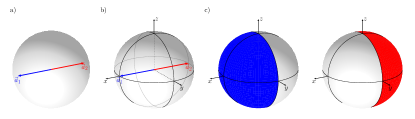
Figure 4: Consider the two-outcome POVM with operators $A^{1/2}_{i|a}=(\mathds{1}\pm\vec{a}_{1}\cdot\vec{\sigma}/2)/2$. a) Here, $\vec{a}_{1}$ can be an arbitrary direction in the Bloch sphere. b) We can choose a coordinate frame in which the $x$-axis is aligned with $\vec{a}_{1}$. c) The conditional probabilities $p(i|a,\vec{\lambda})$ reduce precisely to $p(1|a,\vec{\lambda})=1$ if $\vec{\lambda}\cdot\vec{a}_{1}\geq 0$ and $p(1|a,\vec{\lambda})=0$ if $\vec{\lambda}\cdot\vec{a}_{1}<0$ as indicated with the two colors. Hence, if the outcome $\vec{\lambda}$ of the parent POVM lies in the hemisphere that corresponds to $\vec{a}_{1}$ (blue region) the outcome is always $i=1$ and if it lies in the red region, the outcome will be $i=2$.

An important special case is the one of an (unsharp) projective measurement with two outcomes. Therefore, we have $p_{1}=p_{2}=1$ and $\vec{a}_{2}=-\vec{a}_{1}$, hence $A^{1/2}_{1|a}=(\mathds{1}+\vec{a}_{1}\cdot\vec{\sigma}/2)/2$ and $A^{1/2}_{2|a}=(\mathds{1}-\vec{a}_{1}\cdot\vec{\sigma}/2)/2$. In that case, we can choose the $x$-axis to be aligned with $\vec{a}_{1/2}$, such that in that frame $\vec{a}_{1}=(1,0,0)^{T}$. In this coordinate frame, we can express the function $f(\vec{x})$ as $f(\vec{x})=\Theta(\vec{x}\cdot\vec{a}_{1})+\Theta(-\vec{x}\cdot\vec{a}_{1})=|\vec{x}\cdot\vec{a}_{1}|$. Since $\vec{a}_{1}=(1,0,0)^{T}$, it is clear that $f(\vec{v}_{s_{x}s_{y}s_{z}})=1$ for all eight vectors $\vec{v}_{s_{x}s_{y}s_{z}}=(s_{x},s_{y},s_{z})^{T}$ as required. In addition, note that $\Theta(\vec{v}_{s_{x}s_{y}s_{z}}\cdot\vec{a}_{1})=1$ if $s_{x}=+1$ and $\Theta(\vec{v}_{s_{x}s_{y}s_{z}}\cdot\vec{a}_{1})=0$ if $s_{x}=-1$. Therefore, $\alpha_{1}=\alpha_{2}=0$ and the conditional probabilities translate precisely to $p(1|a,\vec{\lambda})=1$ if $\vec{\lambda}\cdot\vec{a}_{1}\geq 0$ and $p(1|a,\vec{\lambda})=0$ if $\vec{\lambda}\cdot\vec{a}_{1}<0$ (and the analog expression for $i=2$).

D.2 Three-outcome measurements

Another special case is if all the vectors lie in a plane. In particular, this is true if the POVM has only three outcomes since $p_{1}\vec{a}_{1}+p_{2}\vec{a}_{2}+p_{3}\vec{a}_{3}=\vec{0}$ can only be satisfied if all three vectors lie in the same plane. In that case, we can choose the coordinate frame such that $z$ is orthogonal to the plane in which the vectors lie. With that choice of coordinate frame, we can observe that $f(\vec{v}_{s_{x}s_{y}+})=f(\vec{v}_{s_{x}s_{y}-})$ since $\vec{a}_{i}\cdot(0,0,1)^{T}=0$ and therefore the $z$-component of $\vec{v}_{s_{x}s_{y}s_{z}}$ does not affect the value of $f(\vec{v}_{s_{x}s_{y}s_{z}})$. Together with $f(\vec{v}_{s_{x}s_{y}s_{z}})=f(\vec{v}_{-s_{x}-s_{y}-s_{z}})$ (note that $\vec{v}_{s_{x}s_{y}s_{z}}=-\vec{v}_{-s_{x}-s_{y}-s_{z}}$), we can denote $C_{1}:=f(\vec{v}_{+++})=f(\vec{v}_{++-})=f(\vec{v}_{--+})=f(\vec{v}_{---})$ and $C_{2}:=f(\vec{v}_{+-+})=f(\vec{v}_{+--})=f(\vec{v}_{-++})=f(\vec{v}_{-+-})$. As a consequence of the bound in Eq. (16), we obtain $C_{1}+C_{2}\leq 2$. Now we can show that there always exists a rotation around the $z$-axis such that both values $C_{1}$ and $C_{2}$ are smaller or equal to one. If we fix at the beginning a coordinate frame where both values are smaller than one, we can use precisely that frame. On the other hand, if one value (suppose $C_{1}$) is above one, the other one ($C_{2}$) is smaller than one. Now we rotate the coordinate axes. If we rotate by 90 degrees, we map the vector $\vec{v}_{+-+}$ to the vector $\vec{v}_{+++}$ and therefore in the rotated coordinate frame we obtain $\tilde{C}_{1}=f(\vec{\tilde{v}}_{+++})=f(\vec{v}_{+-+})=C_{2}\leq 1$. By the intermediate value theorem and since $f$ is continuous, there is a rotation (with less than 90 degrees) such that $\tilde{C}_{1}=f(\vec{\tilde{v}}_{+++})=1$ which implies that $\tilde{C}_{2}=f(\vec{\tilde{v}}_{+-+})\leq 1$ since $\tilde{C}_{1}+\tilde{C}_{2}\leq 2$ holds for each of these coordinate frames. In this way, we can construct a suitable coordinate frame without relying on the theorem of Ref. [28] but only on the intermediate value theorem.

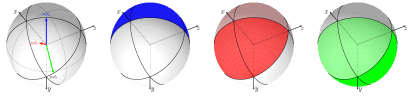
Figure 5: An illustration of $p(i|a,\vec{\lambda})$ for a three-outcome POVM. Here the conditional probabilities do not depend on $z$ due to the choice of the coordinate frame. If $\vec{\lambda}$ is close to one of the colored vectors it is also more likely that this color is produced as an output.

D.3 SIC-POVM

We also want to give an example with a four-outcome measurement, namely a SIC-POVM. We can represent a SIC POVM as follows:

$$\vec{a}_{1} =\begin{pmatrix}0\\ 0\\ 1\end{pmatrix} \vec{a}_{2} =\begin{pmatrix}\sqrt{8}/3\\ 0\\ -1/3\end{pmatrix} \vec{a}_{3} =\begin{pmatrix}-\sqrt{2}/3\\ \sqrt{6}/3\\ -1/3\end{pmatrix} \vec{a}_{4} =\begin{pmatrix}-\sqrt{2}/3\\ -\sqrt{6}/3\\ -1/3\end{pmatrix}$$ (65)

and the coefficients $p_{i}$ are $p_{1}=p_{2}=p_{3}=p_{4}=1/2$. If we choose the coordinate frame such that the four vectors have the above form it is easy to verify that $f(\vec{v}_{s_{x}s_{y}s_{z}})\leq 1$ for each $\vec{v}_{s_{x}s_{y}s_{z}}=(s_{x},s_{y},s_{z})$. See the following table:

i		$\vec{a}_{i}$		+ + +	+ + -	+ - +	+ - -	- + +	- + -	- - +	- - -	$\sum$	$\alpha_{i}$
1 (blue)	(0.000,	0.000,	$1.000)^{T}$	0.5	0	0.5	0	0.5	0	0.5	0	2	0
2 (red)	(0.943,	0.000,	$-0.333)^{T}$	0.305	0.638	0.305	0.638	0	0	0	0	1.886	0.014
3 (green)	(-0.471,	0.816,	$-0.333)^{T}$	0.006	0.339	0	0	0.477	0.811	0	0	1.633	0.046
4 (yelow)	(-0.471,	-0.816,	$-0.333)^{T}$	0	0	0.006	0.339	0	0	0.477	0.811	1.633	0.046
	$f(\vec{v}_{s_{x}s_{y}s_{z}})$	$=\sum_{i}p_{i}$	$\Theta(\vec{v}_{s_{x}s_{y}s_{z}}\cdot\vec{a}_{i})$	0.811	0.977	0.811	0.977	0.977	0.811	0.977	0.811	7.152

Table 1: Caption: Here we represent the functional values of $p_{i}\ \Theta(\vec{v}_{s_{x}s_{y}s_{z}}\cdot\vec{a}_{i})$ for the chosen SIC-POVM. The last row gives the values for the function $f(\vec{v}_{s_{x}s_{y}s_{z}})=\sum_{i}p_{i}\ \Theta(\vec{v}_{s_{x}s_{y}s_{z}}\cdot\vec{a}_{i})$ which is obtained by taking the sum over all $i$. We also calculate every $\alpha_{i}$ in the last column.

i		$\vec{a}_{i}$		+ + +	+ + -	+ - +	+ - -	- + +	- + -	- - +	- - -	$\sum$
1 (blue)	(0.000,	0.000,	$1.000)^{T}$	0.5	0	0.5	0	0.5	0	0.5	0	2
2 (red)	(0.943,	0.000,	$-0.333)^{T}$	0.330	0.641	0.330	0.641	0.003	0.026	0.003	0.026	2
3 (green)	(-0.471,	0.816,	$-0.333)^{T}$	0.088	0.349	0.082	0.010	0.487	0.893	0.010	0.082	2
4 (yelow)	(-0.471,	-0.816,	$-0.333)^{T}$	0.082	0.010	0.088	0.349	0.010	0.082	0.487	0.893	2
				1	1	1	1	1	1	1	1

Table 2: Here we represent the conditional probabilities $p(i|a,\vec{\lambda})$ given the octant in which $\vec{\lambda}=(\lambda_{x},\lambda_{y},\lambda_{z})$ lies (denoted as $s_{x}s_{y}s_{z}$ where $s_{k}=\operatorname{sgn}(\lambda_{k})$ for $k=x,y,z$). Intuitively speaking, they are the same values as in the table above but we fill the rest with noise. The last row is obtained by taking the sum over all $i$ which shows that the probabilities sum to one. A short calculation can also directly verify that $\sum_{s_{x},s_{y},s_{z}=\pm 1}p(i|a,\vec{\lambda})\ G_{s_{x}s_{y}s_{z}}=A^{1/2}_{i|a}$.

Figure 6: (same figure as in the main text) The coloured arrows denote the vectors $p_{i}\vec{a}_{i}$ according to $p_{i}=1/2$ and the vectors $\vec{a}_{i}$ given above. The right part of the figure represents the conditional probabilities given in the table above. If for example, $\vec{\lambda}$ lies in the octant that corresponds to "-++" ($s_{x}=-1$, $s_{y}=s_{z}=+1$) the outcome is $i=1$ (blue) with $p(1|a,\vec{\lambda})=0.5$, $i=2$ (red) with $p(2|a,\vec{\lambda})=0.003$, $i=3$ (green) with $p(3|a,\vec{\lambda})=0.487$, and $i=4$ (yellow) with $p(4|a,\vec{\lambda})=0.01$. Therefore, the outcome is most likely to be either $i=1$ or $i=3$.

D.4 Every coordinate frame is possible for SIC-POVMs

However, it turns out that any other choice of coordinate frame would be equally valid. Therefore, in a different coordinate frame, the functions for the conditional probabilities would change but a simulation is still possible. Indeed, we can prove that $f(\vec{x})\leq 1$ for every vector $\vec{x}$ with $|\vec{x}|\leq\sqrt{3}$. Therefore for every choice of coordinate frame the vectors $\vec{v}_{s_{x}s_{y}s_{z}}=(\pm 1,\pm 1,\pm 1)$ satisfy $f(\vec{v}_{s_{x}s_{y}s_{z}})\leq 1$ since $|\vec{v}_{s_{x}s_{y}s_{z}}|=\sqrt{3}$. For the SIC-POVM the function becomes the following:

$$f(\vec{x})=\sum_{i}p_{i}\ \Theta(\vec{x}\cdot\vec{a}_{i})=\frac{\Theta(\vec{x}\cdot\vec{a}_{1})+\Theta(\vec{x}\cdot\vec{a}_{2})+\Theta(\vec{x}\cdot\vec{a}_{3})+\Theta(\vec{x}\cdot\vec{a}_{4})}{2}$$ (66)

Depending on the region where $\vec{x}$ lies, some of the terms $\vec{x}\cdot\vec{a}_{i}$ are positive and some of them are negative. We show that in any case, $f(\vec{x})\leq 1$ if $|\vec{x}|\leq\sqrt{3}$. Suppose only the term $\vec{x}\cdot\vec{a}_{1}$ is positive and the remaining three terms $\vec{x}\cdot\vec{a}_{i}$ are negative (this happens for instance if $\vec{x}=(x,0,0)$). If this is the case, the function becomes

$$f(\vec{x})=\frac{\Theta(\vec{x}\cdot\vec{a}_{1})}{2}=\frac{\vec{x}\cdot\vec{a}_{1}}{2}\leq\frac{|\vec{x}|\cdot|\vec{a}_{1}|}{2}=\frac{|\vec{x}|}{2}$$ (67)

where we used the Cauchy-Schwarz inequality and $|\vec{a}_{1}|=1$. The same argument holds if one of the other terms is positive and the remaining three are negative. Now consider, that the two terms $\vec{x}\cdot\vec{a}_{1}$ and $\vec{x}\cdot\vec{a}_{2}$ are positive, and the remaining two are negative. Then the function becomes:

$$f(\vec{x})=\frac{\Theta(\vec{x}\cdot\vec{a}_{1})+\Theta(\vec{x}\cdot\vec{a}_{2})}{2}=\frac{\vec{x}\cdot\vec{a}_{1}+\vec{x}\cdot\vec{a}_{2}}{2}=\frac{\vec{x}\cdot(\vec{a}_{1}+\vec{a}_{2})}{2}\leq\frac{|\vec{x}|\cdot|\vec{a}_{1}+\vec{a}_{2}|}{2}=\frac{|\vec{x}|\cdot\sqrt{\frac{4}{3}}}{2}=\frac{|\vec{x}|}{\sqrt{3}}$$ (68)

Here we used again the Cauchy-Schwarz inequality and note that $\vec{a}_{1}+\vec{a}_{2}=(\sqrt{8}/3,0,2/3)^{T}$ (hence $|\vec{a}_{1}+\vec{a}_{2}|=\sqrt{4/3}$). Due to symmetry reasons (or by a similar calculation), the same applies to any other combination of these four terms, in which exactly two of them are positive.

In the case where three terms are positive, we obtain similarly (note that $\vec{a}_{1}+\vec{a}_{2}+\vec{a}_{3}+\vec{a}_{4}=\vec{0}$):

$$f(\vec{x})=\frac{\Theta(\vec{x}\cdot\vec{a}_{1})+\Theta(\vec{x}\cdot\vec{a}_{2})+\Theta(\vec{x}\cdot\vec{a}_{3})}{2}=\frac{\vec{x}\cdot(\vec{a}_{1}+\vec{a}_{2}+\vec{a}_{3})}{2}=\frac{\vec{x}\cdot(-\vec{a}_{4})}{2}\leq\frac{|\vec{x}|\cdot|\vec{a}_{4}|}{2}=\frac{|\vec{x}|}{2}$$ (69)

If none of the terms is positive, the function becomes clearly $f(\vec{x})=0$. If all of the terms are positive, the function becomes also $f(\vec{x})=(\vec{x}\cdot(\vec{a}_{1}+\vec{a}_{2}+\vec{a}_{3}+\vec{a}_{4}))/2=0$ since $\vec{a}_{1}+\vec{a}_{2}+\vec{a}_{3}+\vec{a}_{4}=\vec{0}$. (However, by geometric arguments there are no vectors except $\vec{x}=\vec{0}$ where either none or all of the terms are positive.) One can see that, no matter in which case we are, for every vector with $|\vec{x}|\leq\sqrt{3}$ the function satisfies $f(\vec{x})\leq 1$, and therefore every coordinate frame can be chosen.