Gravitational Wave non-Gaussianity from trans-Planckian Quantum Noise

Abstract

We examine the effect of a trans-Planckian phase on the dynamics of inflationary tensor perturbations. To remedy the fact that this regime is not fully captured by standard perturbation theory, we introduce an effective quantum noise source, whose role is regulated by the energy scale $\Lambda$. The presence of the source modifies the initial conditions for the tensor modes, leaving a distinct imprint. We study the amplitude and shape of the gravitational wave bispectrum of the model and compare these with their counterparts obtained under the assumptions of Bunch-Davies initial conditions and $\alpha$-vacua states. Depending on the value of the scale $\Lambda$, we find distinctive signatures associated with both the bispectrum shape and the non-linear parameter $f_{\rm NL}$.

1 Introduction

Inflation stands as one of the main pillars of our current understanding of cosmology. It solves the puzzles associated with the Hot Big Bang model and provides a mechanism to seed the growth of structure [1, 2, 3, 4]. These successes of the inflationary paradigm notwithstanding, there is plenty we do not yet know about inflation. Most notably, a host of wildly different inflationary models are compatible with current observations, CMB experiments being those providing the most stringent constraints to date. The key questions that remain unanswered are the energy scales involved during inflation and the field content of the inflationary Lagrangian. In current parlance, we do not yet know at what energy the “cosmological collider” operates nor do we have crucial information on the (self-)interactions characterising the inflationary particle zoo.

Remarkably, an unprecedented array of cosmological probes is scheduled to become operational in the next decade: it promises to transform the current picture of the early universe and address some of the most pressing issues. What is perhaps most exciting is the prospect of testing more than 20 decades in the frequency of the gravitational wave (GW) signal in the coming years. At CMB scales we will soon be able to test the energy scale of inflation by ever-more-stringent bounds on the tensor to scalar ratio $r$ ($\sigma_{r}\sim 10^{-2}$ for e.g. CMB-S3 experiments [5, 6] and $\sigma_{r}\sim 10^{-3}$ for CMB-S4 [7, 8] and LiteBIRD [9]). Large-scale structure experiments such as Euclid and the Rubin Observatory will constrain inflationary interactions down do $\sigma_{f_{\rm NL}}\sim({\rm a\,few})$, whilst 21cm cosmology promises even more down the line [10]. Given that primordial gravitational waves are a universal prediction of inflation, one ought to mention the possibilities afforded by pulsar timing arrays [11, 12, 13, 14, 15, 16, 17, 18, 19, 20, 21], and ground and space-based interferometers [22, 11, 23, 24].

It is worthwhile to also widen the overall perspective and recall that, although the structure we observe today may originate from magnified quantum fluctuations, current data is compatible with both a classical and quantum origin of the patterns we see imprinted in our observables. Intriguingly, key insights on the quantum vs classical origin may be inferred from the structure of the cosmological correlation functions [25, 26]. Cosmological correlators are also sensitive to the choice of the vacuum or initial state for inflation [27]. In this work, we will go beyond the standard Bunch-Davies choice for the vacuum and explore other well-motivated initial conditions, such as those known as $\alpha$-vacua [28, 29, 30, 31, 32, 33, 34, 35, 36, 37, 38, 27]. Inflation from non-adiabatic initial states comes with specific signatures, including at the level of gravitational wave non-Gaussianities [33, 39]. With respect to existing literature, our work here explores the effect of a non-zero anisotropic stress tensor sourcing gravitational wave production. Given that the inflationary energy regime can be perilously close to the Planck scale, we will also be concerned with the trans-Planckian problem (see e.g. [40, 41, 42]) and the fact that the standard description of inflation may break down at such energies. We shall tackle the effect of trans-Planckian physics on GWs by adopting an open quantum system description where tensor perturbations effectively interact with their environment. We will model the effect of the environment by means of an anisotropic stress tensor which accounts for the dynamics above an energy threshold $\Lambda$ [43]. Some of us argued in [43] that such a source is compatible with a nearly scale-invariant GW spectrum at CMB scales, in full agreement with the latest observations [44]. In this work, we will investigate the gravitational wave non-Gaussianity stemming from such a setup.

We will add one by one the various layers that make up our system. We start with a simple scalar field minimally coupled to gravity and briefly review the corresponding tensor non-Gaussianity. The next step consists of considering non-adiabatic initial states, specifically $\alpha$-vacua. Last, we consider the effect of non-zero anisotropic stress whose dynamics are regulated by the dimensional quantity $\Lambda$.

This paper is structured as follows. In Section 2.1, we provide a review of the dynamics associated with the tensor modes during the inflationary period. Additionally, we present a thorough analysis of the essential methodologies required for investigating the bispectrum. Furthermore, we present the outcomes obtained specifically for the Bunch-Davies vacuum selection. In Section 2.2, we introduce the concept of degeneracy in the vacuum state and highlight the key distinctions from the previous section by incorporating a cut-off energy scale for the vacuum selection. Lastly, in Section 3, we extend the scope of our findings by incorporating a trans-Planckian source that impacts the shape of the bispectrum leaving distinct imprints.

2 Tensor Bispectrum: with and without a cut-off energy scale

2.1 Bunch-Davies vacuum

In this section, we will briefly review the results on tensor non-Gaussianity in the case of the standard Bunch Davies vacuum. Naturally, the starting point for the tree-level power spectrum is the quadratic action describing the behaviour of the tensor degrees of freedom of general relativity, whilst the cubic action is necessary to arrive at the three-point function or, equivalently, the bispectrum. Let us consider as the inflationary Lagrangian that of single-field slow-roll, i.e. general relativity minimally coupled to a “matter” Lagrangian $\mathcal{L}_{\rm matter}$:

$$\mathcal{L}=\mathcal{L}_{\rm EH}+\mathcal{L}_{matter}=\sqrt{-g}\Bigg{[}\frac{1}{2}R+\frac{1}{2}g^{\mu\nu}\partial_{\mu}\partial_{\nu}\phi-V(\phi)\Bigg{]}\;,$$ (2.1)

where we set $M_{\rm Pl}$ to one. Expanding Eq. (2.1) around the FLRW solution up to the second order, focusing on standard tensor fluctuations, one obtains the following linearized equations of motion:

$$h^{\prime\prime}_{\bf k}+2\mathcal{H}h^{\prime}_{\bf k}+k^{2}h_{\bf k}=16\pi Ga^{2}\Pi_{\bf k}(\tau)$$ (2.2)

where the anisotropic stress term $\Pi$ in the RHS is the source term, easily derived from Eq.(2.1). Here and in Section 2.2 we shall work within the context of single-field slow-roll inflation and will therefore neglect the subleading correction due to the $\Pi$ term. By virtue of using the re-scaled field $v\equiv a(\tau)h$ in Eq. (2.2), one arrives at the Mukhanov-Sasaki equation:

$$v^{\prime\prime}_{\textbf{k}}+\Big{(}k^{2}-\frac{a^{\prime\prime}}{a}\Big{)}v_{\textbf{k}}=0\;,$$ (2.3)

which admits as a solution the following combination of the Bessel functions:

$$v_{k}(\tau)=A_{k}Y_{\nu}(k,\tau)+B_{k}J_{\nu}(k,\tau)\;,$$ (2.4)

where $\nu\approx 3/2$ for a quasi de Sitter background (up to the first slow-roll corrections).

Figure 1: Representation of the three configurations for the momenta $(k_{1},k_{2},k_{3})$. Case (a): Equilateral configuration meaning that $k_{1}\approx k_{2}\approx k_{3}$. Case (b): Squeezed configuration, $k_{3}\ll k_{1}\approx k_{2}$ . Case (c): Folded shape, $k_{3}\approx k_{1}+k_{2}$.

In the following, we will employ the in-in formalism to tackle second and higher-order correlation functions. The tree-level contribution to the tensor three-point function reads:

$${}_{in}\langle 0|\hat{h}^{s_{1}}_{\mathbf{k}_{1}}(\tau)\hat{h}^{s_{2}}_{\mathbf{k}_{2}}(\tau)\hat{h}^{s_{3}}_{\mathbf{k}_{3}}(\tau)|0\rangle_{in}=-i\int^{\tau}_{-\infty}d\tau^{\prime}a(\tau^{\prime})\langle\Big{[}\hat{h}^{s_{1}}_{\mathbf{k}_{1}}(\tau)\hat{h}^{s_{2}}_{\mathbf{k}_{2}}(\tau)\hat{h}^{s_{3}}_{\mathbf{k}_{3}}(\tau),H^{(3)}_{I}(\tau^{\prime})\Big{]}\rangle\;,$$ (2.5)

where the operator $\hat{h}$ is such that $\hat{h}_{\textbf{k}}=h_{\textbf{k}}\hat{a}_{\textbf{k}}+h^{*}_{-\textbf{k}}\hat{a}^{{\dagger}}_{-\textbf{k}}$. The gravitational self-interactions of general relativity making up the cubic Hamiltonian in the interaction picture are given by [45, 46, 32, 47]:

$$H^{(3)}_{I}(\tau)=-\frac{1}{M^{4}_{Pl}}\int d^{3}x\,a(\tau)\Big{(}h_{ik}h_{jl}-\frac{1}{2}h_{ij}h_{kl}\Big{)}\partial_{k}\partial_{l}h_{ij}\;.$$ (2.6)

Following standard practice (see [48, 49, 38]), we write the spectrum as:

$$\langle h_{ij}(\textbf{k}_{1})h_{kl}(\textbf{k}_{2})\rangle=(2\pi)^{3}\delta^{(3)}(\textbf{k}_{1}+\textbf{k}_{2})\mathcal{P}_{ij,kl}(\textbf{k})$$ (2.7)

where we defined the last term on RHS as $\mathcal{P}_{ij,kl}(\textbf{k})=|h_{\textbf{k}}|^{2}\sigma_{ij,kl}(\textbf{k})$, where the $\sigma$ tensor encodes all the information about the polarization tensors:

$$\sigma_{ij,kl}(\textbf{k})=\sum_{s}e^{(s)}_{ij}e^{*(s)}_{kl}$$ (2.8)

and the bispectrum as:

$$\langle h_{i_{1}j_{1}}(\mathbf{k}_{1})h_{i_{2}j_{2}}(\mathbf{k}_{2})h_{i_{3}j_{3}}(\mathbf{k}_{3})\rangle=(2\pi)^{7}\delta^{3}(\textbf{k}_{1}+\textbf{k}_{2}+\textbf{k}_{3})\mathcal{P}^{2}_{t}\tilde{\mathcal{A}}_{i_{1}j_{1}i_{2}j_{2}i_{3}j_{3}}$$ (2.9)

where $\mathcal{P}^{2}_{t}$ is the amplitude of the standard tensor power spectrum i.e. $\mathcal{P}_{t}=H^{2}/(2\pi M_{Pl})^{2}$ and the term $\tilde{\mathcal{A}}_{i_{1}j_{1}i_{2}j_{2}i_{3}j_{3}}$ can be decomposed into two parts:

$$\tilde{\mathcal{A}}_{i_{1}j_{1}i_{2}j_{2}i_{3}j_{3}}=\mathcal{A}\times P_{i_{1}j_{1}i_{2}j_{2}i_{3}j_{3}}\;.$$ (2.10)

The tensorial part of the last term is given by:

$$P_{i_{1}j_{1}i_{2}j_{2}i_{3}j_{3}}=\sigma_{i_{1}j_{1},kl}(\textbf{k})\sigma_{ij,kl}(\textbf{k})\Big{[}k_{3k}k_{3l}\sigma_{ij,kl}(\textbf{k}_{3})-\frac{1}{2}k_{3i}k_{3k}\sigma_{ij,kl}(\textbf{k}_{3})\Big{]}+\rm{perms.of}\{1,2,3\}$$ (2.11)

and so, overall, it depends upon the specific polarization state $(s_{1},s_{2},s_{3})$ we chose for the basis, i.e. $P_{i_{1}j_{1}i_{2}j_{2}i_{3}j_{3}}\equiv P^{s_{1}s_{2}s_{3}}$. To make contact with the literature, we will always make use of the (+++) polarization. The term $\mathcal{A}$ is instead referred to as the scalar counterpart which can be integrated out from the tensorial factor and can be computed by means of the in-in formula we showed above. Then, taking just the single polarization +++, and defining $K_{T}=k_{1}+k_{2}+k_{3}$ we obtain:

$$P^{+++}=\frac{K^{5}_{T}}{128(k_{1}k_{2}k_{3})^{2}}\Big{[}K^{3}_{T}-\sum_{i\neq j}k^{2}_{i}k_{j}-4k_{1}k_{2}k_{3}\Big{]}\;.$$ (2.12)

From now on, once we set a given tensor polarization state (i.e. the $P^{s_{1}s_{2}s_{3}}$ function ) we will just have to compute the $\mathcal{A}$ factor.

From Eqs. (2.5),(2.6) one readily derives

$${}_{in}\langle 0|\hat{h}^{s_{1}}_{\mathbf{k}_{1}}(\tau)\hat{h}^{s_{2}}_{\mathbf{k}_{2}}(\tau)\hat{h}^{s_{3}}_{\mathbf{k}_{3}}(\tau)|0\rangle_{in}=\lim_{k\tau\rightarrow 0}\frac{1}{M^{4}_{Pl}}.\Im\Big{[}h_{\textbf{k}_{1}}(\tau)h_{\textbf{k}_{2}}(\tau)h_{\textbf{k}_{3}}(\tau)\int^{\tau}_{-\infty}d\tau^{\prime}h_{\textbf{k}_{1}}(\tau^{\prime})h_{\textbf{k}_{2}}(\tau^{\prime})h_{\textbf{k}_{3}}(\tau^{\prime})\Big{]}$$ (2.13)

where, in the last formula, we have temporarily re-instated the Planck mass in order to make an easy comparison with the literature. Implementing the Bunch-Davies condition for the vacuum is tantamount to requiring the following behaviour deep inside the horizon,

$$v_{k\gg aH}\rightarrow\frac{e^{-ik\tau}}{\sqrt{2k}}\;.$$ (2.14)

This prescription is equivalent to asking the mode functions to be in their flat (Minkowskian) configuration at the beginning of their evolution. As we shall see shortly, this corresponds to the “minimal” choice for the Bogoliubov coefficients $A_{k}$ and $B_{k}$ (i.e. $A_{k}=1$ and $B_{k}=0$). The choice of the BD vacuum is further motivated by the fact it is a quantum attractor for the system [50]. From the previous expression, one arrives at the following value for the amplitude of tensor non-Gaussianities,

$$\mathcal{A}_{BD}=-\Big{(}\frac{H}{M_{Pl}}\Big{)}^{2}\frac{\Big{[}\sum_{i}k^{3}_{i}+2\sum_{i\neq j}k^{2}_{i}k_{j}\Big{]}}{8K^{2}_{T}(k_{1}k_{2}k_{3})^{3}}\ \;,$$ (2.15)

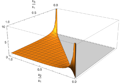
where the subscript “BD” underscores the current choice of the vacuum, in contradistinction to the options we will explore in Section 2.2. The momenta dependence of the bispectrum, that is, the shape of non-Gaussianity, is illustrated in Fig. 2, which clearly shows a profile that is very well described by the local template [51]. It is convenient at this stage to define the non-linear parameter $f_{\rm NL}$ for the tensor three-point function. Following standard practice [39, 52], we define it as:

$$f_{\rm NL}=\frac{\tilde{\mathcal{A}}_{+++}}{P_{t}(k_{1})P_{t}(k_{2})+{\rm perm.}}\;,$$ (2.16)

where the numerator represents the bispectrum :

$$\tilde{\mathcal{A}}_{+++} =\frac{\left(k_{1}^{3}-\left(k_{2}+k_{3}\right)k_{1}^{2}-\left(k_{2}-k_{3}\right){}^{2}k_{1}+\left(k_{2}-k_{3}\right){}^{2}\left(k_{2}+k_{3}\right)\right)}{1024k_{1}^{5}k_{2}^{5}k_{3}^{5}}\times$$ (2.17)

$$\times\left(k_{1}^{3}+2\left(k_{2}+k_{3}\right)k_{1}^{2}+2\left(k_{2}^{2}+k_{3}k_{2}+k_{3}^{2}\right)k_{1}+k_{2}^{3}+k_{3}^{3}+2k_{2}k_{3}^{2}+2k_{2}^{2}k_{3}\right)\;.$$ (2.18)

We stress here that the definition of $f_{\rm NL}$ is not univocal as one may simply build the estimator associated with any given definition. Depending on the shape of the bispectrum, one may define different non-linear parameters. One typically tries to capture, with a given $f_{\rm NL}$ definition, a finite well-defined amplitude that best signals the departure from Gaussianity. In what follows we shall also make use of a complementary definition to the one given in Eq. (2.16), namely

$$f^{\textit{fold}}_{\rm NL}=\frac{\tilde{\mathcal{A}}_{+++}}{(P_{t}(k_{1})P_{t}(k_{2})+\textit{perm.})+3(P_{t}(k_{1})P_{t}(k_{2})P_{t}(k_{3}))^{2/3}-[(P_{t}(k_{1})P^{2}_{t}(k_{2})P^{3}_{t}(k_{3}))^{1/3}+\textit{perm.}]},$$ (2.19)

where the $P_{t}$ we used for $f_{\rm NL}$ is the dimensional definition for the power spectrum, i.e. $k^{3}P_{t}=\mathcal{P}_{t}$. The quantity $f^{\textit{fold}}_{\rm NL}$ is indeed, particularly useful whenever the bispectrum profile is of the folded type, i.e. when the maxima of the shape-function correspond to a whole line in the $(k_{2}/k_{1},k_{3}/k_{1})$ plane.

To provide an explicit example, in the case of Bunch-Davies vacuum, for Eq. (2.16) one immediately finds

$$f^{BD}_{\rm NL}= \frac{K_{T}^{3}\left(2k_{2}-K_{T}\right)\left(2k_{3}-K_{T}\right)\left(2k_{2}+2k_{3}-K_{T}\right)}{16384k_{1}^{2}k_{2}^{2}k_{3}^{2}\left(k_{1}^{3}+k_{2}^{3}+k_{3}^{3}\right)}\times$$

$$\times\left(-k_{2}K_{T}^{2}-k_{3}K_{T}^{2}+k_{2}^{2}K_{T}+k_{3}^{2}K_{T}+k_{2}k_{3}^{2}+k_{2}^{2}k_{3}+K_{T}^{3}\right)$$

and a corresponding expression is found employing Eq. (2.19).

As we can notice, the vanilla model predicts fixed values for the non-linear parameter. The only two configurations in which the $f_{\rm NL}$ parameter is effectively non-zero, are the equilateral and the squeezed ones (the folded limit, for the BD initial condition, is always null in either definition for the $f_{\rm NL}$ we take). However, as we shall see, the folded limit is the one which is more sensitive to a variation of the initial conditions.

Figure 2: Plot of the shape function $\mathcal{A}$ Eq. 2.18 multiplied by $(k_{2}/k_{1})(k_{3}/k_{1})$ to match the other results in literature [48]. The plot is normalized to unity for equilateral configuration.

We stress that yet another definition of $f^{\rm tens}_{\rm NL}$ is widely in use (see e.g. [33]):

$$\tilde{f}_{\rm NL}=\frac{\tilde{\mathcal{A}}_{+++}}{P_{\zeta}(k_{1})P_{\zeta}(k_{2})+{\rm perm.}}=\frac{\tilde{\mathcal{A}}_{+++}}{P_{t}(k_{1})P_{t}(k_{2})+{\rm perm.}}r^{2}\equiv f_{\rm NL}r^{2}$$ (2.20)

and a corresponding definition is naturally in place, e.g., the folded case. In Table 1 we show the results depending upon the tensor-to-scalar ratio $r$.

Table 1: Values of $\tilde{f}_{\rm NL}$ obtained for the three different configurations and the BD vacuum. We obtained these numbers by setting $k_{\text{long}}\approx 10^{-3}k_{\text{short}}$ for the squeezed limit.

$\tilde{f}_{NL}$ for standard GR + BD vacuum
Equilateral	Squeezed
$0.00933\times r^{2}$	$0.00293\times r^{2}$

2.2 $\alpha$ vacua and fixed initial time choice

Having introduced all the necessary tools in the previous section, we can now tackle generalized/mixed states in the early Universe. Since the inflationary dynamics take place in an approximate de Sitter background, we have a family of different, equivalent, vacua. This is due to the lack of time–like Killing vectors in a general dynamical background see e.g. [53].

The general solution of the Mukhanov-Sasaki equation can be written in terms of Hankel functions as

$$h_{k}(\tau)=\frac{A_{k}}{a(\tau)}\frac{e^{-ik\tau}}{\sqrt{2k}}\Big{(}1-\frac{i}{k\tau}\Big{)}+\frac{B_{k}}{a(\tau)}\frac{e^{ik\tau}}{\sqrt{2k}}\Big{(}1+\frac{i}{k\tau}\Big{)}\equiv A_{k}u_{k}+B_{k}u^{*}_{k},$$ (2.21)

where the two time-independent parameters $A_{k}$ and $B_{k}$ are known as Bogoliubov coefficients. These coefficients are bound to the normalization condition imposed by requiring the conservation of the canonical relations for the ladder operators $a_{\textbf{k}}$ and $a^{{\dagger}}_{\textbf{k}}$, that is, $[a_{\textbf{k}^{\prime}},a^{{\dagger}}_{\textbf{k}}]=\delta^{3}(\textbf{k}^{\prime}-\textbf{k})$. As a result, one finds:

$$|A_{k}|^{2}-|B_{k}|^{2}=1\;.$$ (2.22)

This relation allows for a simple parametrization in terms of hyperbolic functions, giving, for the wavefunction $h$:

$$h_{k}(\tau)=u_{k}\cosh{\alpha}+u^{*}_{k}e^{i\beta}\sinh{\alpha},$$ (2.23)

where the two parameters $\alpha,\beta$ can vary in the respective range: $\alpha\in[0,+\infty)$ and $\beta\in(-\pi,\pi)$.

We note here that non-zero values for $\beta$ would break time-reversal invariance so that the quantum state wouldn’t be invariant under the symmetry group $SO(4,1)$. Setting set $\beta=0$ is also necessary in order to smoothly reduce to the choice of a Bunch-Davies vacuum. For a complete treatment of the properties of the vacua in quasi-de Sitter (dS) and mixed states, see [28] as well as [54, 39, 37].

At this stage one typically converges towards specific combinations of the Bogoliubov coefficients, see [54, 55] for some well-motivated examples. In this section, we shall take the point of view of [56, 57] which underscores the fact that initial conditions are often imposed for very large momenta. In this regime, one does not have complete control of the quantum field theory description. It is then convenient to set a cutoff scale $\Lambda$ that limits the remit of the standard treatment. One may equivalently identify the corresponding (conformal) time $\bar{\tau}$ defined as:

$$\bar{\tau}_{k}=-\frac{\Lambda}{kH}\;$$ (2.24)

Additional related possibilities have been considered in [58]. The quantization procedure is standard, with the caveat that the vacuum annihilation holds at a precise time in the evolution,

$$\hat{a}_{\textbf{k}}(\bar{\tau}_{k})|0\rangle=0\;,$$ (2.25)

something commonly known in literature [34, 56, 57, 54] as instantaneous vacuum. One quickly arrives [57] at the following expression for the Bogoliubov coefficients,

$$A_{k}=\sqrt{1+B^{2}_{k}}\qquad\qquad B_{k}=\frac{H}{2\Lambda}\;.$$ (2.26)

Up to slow-roll corrections, both coefficients are not explicitly dependent on the scale $k$. The key quantity is the $H/\Lambda$ ratio, with $H$ a good proxy for the energy scale of inflation and $\Lambda$ signalling when quantum gravitational effects become important. The resulting two-point function is

$$P^{f.t.}=P^{0}_{t}\Big{[}1+\frac{H}{\Lambda}\sin{\frac{\Lambda}{H}}\Big{]}\;,$$ (2.27)

where the oscillating feature regulated by $H/\Lambda$ is completely negligible for typical (i.e. large) values of $\Lambda$. We can now move on to explore the effects of a non-trivial initial state on gravitational wave non-Gaussianities. We will employ the very same framework we described in Section 2.2 to estimate the non-linear parameter and the bispectrum shape function.

Figure 3: Plot of the shape function $\mathcal{A}$ Eq. A.1 multiplied by $(k_{2}/k_{1})(k_{3}/k_{1})$ . The plot is normalized to unity for equilateral configuration.

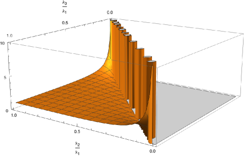
The shape function in Fig. 3 peaks along the diagonal line of the $(k_{2}/k_{1},k_{3}/k_{1})$ plane. This behaviour is characteristic of the so-called folded shape and it has been shown to arise e.g. in the scalar sector in the case of non-BD vacua ([59, 46, 39, 35]). This contribution is a characteristic signature of the presence of a non-zero $\beta_{k}$ coefficient which is responsible for the particle number density ([60, 46]). When dealing with this quantity it turns out to be convenient to introduce a suitable momentum cut-off $\omega$ and corresponding regularized momentum $\textbf{k}_{1}=\textbf{k}_{2}+\textbf{k}_{3}+\omega$, following a procedure that removes any unphysical divergence [46]. Our explicit computation arrives at the same momenta behaviour obtained in [39]. One difference is that, in place of the geometrical $\alpha$ parameter for the parametrization of the initial quantum state, we choose to highlight instead the precise dependence on the energy scale $\Lambda$. In Appendix A we report the explicit expression for both the $f_{\rm NL}$ parameter and the Bispectrum shape function $\mathcal{A}$.

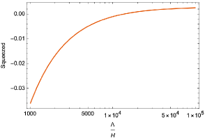
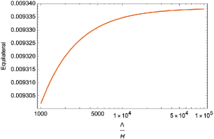
Inspection of Eq. (A.2) reveals the expected dependence of the non-linear parameter on the $\Lambda/H$ ratio. In Fig. 4 we plot the “running” of different configurations as a function of this ratio with a cut-off energy limited by the Planck mass and the Hubble rate limited to be at most $10^{13}{\rm GeV}$. The non-linear parameter may acquire negative values in the squeezed configuration. In every configuration, when $\Lambda$ approaches the Planck mass the non-linear parameter values approach the predictions obtained in the standard case.

Figure 4: Evolution of the $f_{\rm NL}$ parameter as a function of the ratio $\Lambda/H$ for the equilateral and squeezed configurations.

3 Stochastic source

In this section, we shall model the physics that may result, for example, from the presence of additional degrees of freedom sourcing the tensor sector. The anisotropic stress tensor in the GW equation encodes such contributions. Negligible in the standard single-field slow-roll scenario, these may play a leading role in a host of (pre-)inflationary realizations.

One may start from the notion that modes created at very early times have necessarily experienced a trans-Planckian regime [40, 41, 42, 56] on which we have limited access.

Following the approach of [43] we will account for the physics stemming from a trans-Planckian regime through the use of a stochastic source which, at the Lagrangian level, is formally an interaction between the tensor field $h_{ij}$ and an effective operator $\Pi_{ij}$. The main result of the work in [43] is that the prediction for the amplitude of the gravitational wave power spectrum from the BD vacuum is just a particular case in a continuous spectrum of possibilities depending on the $\Lambda/H$ ratio. Much as in [43], our motivations are the following. The description of primordial quantum perturbations cannot be treated as a closed quantum system, but rather an open one. This means that the linear approximation for the perturbations is not adequate, especially when the physical modes approach a given cut-off scale, close to a pure quantum gravitational regime, i.e. $k/a(\tau)\approx\Lambda$. One can consider such non-linearities, in manifold ways. First, one can naturally take tackle higher order perturbation theory. An alternative approach is to describe non-linearities by means of collective forces, i.e. adopt the the mean-field treatment. The latter one will be our approach: it consists in a parametrization of the source term $\Pi_{ij}$ as a Gaussian, stochastic, time - uncorrelated, term with possibly an explicit $k$ dependence. This term ought to switch off at the time $\bar{\tau}_{k}$, when perturbations become sub-Planckian and both GR and the linear regime can be trusted:

$$h^{\prime\prime}_{k}+2\mathcal{H}h^{\prime}_{k}+k^{2}h_{k}=16\pi Ga^{2}\,\Pi_{k}~{}~{}~{} \tau<\bar{\tau}_{k}$$ (3.1)

$$h^{\prime\prime}_{k}+2\mathcal{H}h^{\prime}_{k}+k^{2}h_{k}=0~{}~{}~{}~{}~{}~{}~{}~{}~{}~{}~{}~{}~{} \tau>\bar{\tau}_{k}.$$ (3.2)

The source term is treated as a quantum object much as are tensor fluctuations. As standard, we introduce the ladder operators

$$\hat{\Pi}^{r}_{\textbf{k}}(\tau)=\Pi_{k}(\tau)\hat{a}^{r}_{\textbf{k}}+\Pi^{*}_{k}(\tau)\hat{a}^{r{\dagger}}_{-\textbf{k}}\;.$$ (3.3)

Here too, we follow closely the same approach of [43] where the sea from which the trans-Planckian modes emerge is realized as a Brownian environment, and the source is fully specified by the following conditions:

$$\langle\Pi_{k}(\tau)\rangle =0$$ (3.4)

$$\langle\Pi_{k}(\tau)\Pi_{k}^{*}(\tau^{\prime})\rangle =\Lambda^{6}F(k)\delta(\tau-\tau^{\prime})\;,$$ (3.5)

where we have introduced a dimensionful normalization constant in the two-point function for the noise. Note that, in the current context the brackets have a double role: the usual expectation value over quantum state configurations and the statistical ensemble average over stochastic configurations of the noise. Here we will limit the analysis to a white noise spectrum $F(k)=1$. Further analysis considering the black hole plasma model described in [43] will be considered elsewhere.

The global solution for $h$ is then obtained by implementing standard matching conditions:

$$\lim_{\tau\rightarrow\bar{\tau_{k}}^{-}}h_{k}(\tau) =\lim_{\tau\rightarrow\bar{\tau_{k}}^{+}}h_{k}(\tau)$$ (3.6)

$$\lim_{\tau\rightarrow\bar{\tau_{k}}^{-}}h^{\prime}_{k}(\tau) =\lim_{\tau\rightarrow\bar{\tau_{k}}^{+}}h^{\prime}_{k}(\tau).$$ (3.7)

The general solution of the non-homogeneous Eq. (3.1) is given by:

$$h_{k}(\tau)=\frac{16\pi G}{a(\tau)}\,\int^{\tau}_{-\infty}d\tau^{\prime}a(\tau^{\prime})G_{k}(\tau,\tau^{\prime})\Pi_{k}(\tau^{\prime}),$$ (3.8)

where the Green’s function $G_{k}$ is (see e.g. [61]):

$$G_{k}(\tau,\tau^{\prime})=\frac{e^{-ik(\tau+\tau^{\prime})}}{2k^{3}{\tau^{\prime}}^{2}}\Big{[}e^{2ik\tau}(1-ik\tau)(-i+k\tau^{\prime})+e^{2ik\tau^{\prime}}(1+ik\tau)(i+k\tau^{\prime})\Big{]}\Theta(\tau-\tau^{\prime}).$$ (3.9)

The matching of the solution across $\bar{\tau}$ enforces specific conditions on the Bogoliubov coefficients $A_{k},B_{k}$. Interestingly, from this point of view a non-homogeneous equation in the trans-Planckian regime is equivalent to the selection of a non-Bunch-Davies initial state, see [43] for a thorough study of such equivalence.

Figure 5: Characteristic shape of the bispectrum in the presence of a stochastic source.

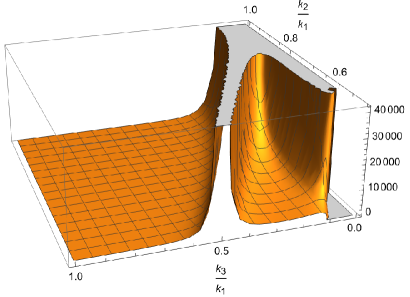
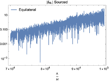
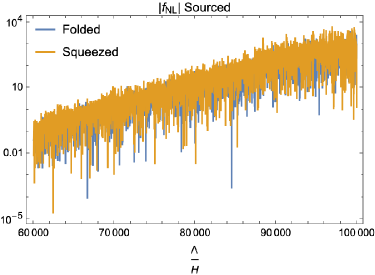
As one can see in Fig. 6 and Fig. 7 the most significant non-linear parameters are those in the squeezed and the folded limits.

Finally, we can conclude that this class of models can support large tensor non-Gaussianities.

Figure 6: LogPlot of the non-linear parameter for the equilateral configuration.

Figure 7: LogPlot of the $|f_{\rm NL}|$ parameter for the squeezed and folded configurations.

4 Conclusions

The standard treatment of cosmological observables from the very early universe is often oblivious to pre-inflationary dynamics. This is not surprising given that, despite great progress e.g. in string theory, a predictive and testable UV complete theory for gravitational interactions remains elusive. In order to try and include pre-inflationary physics in our description, one may codify the effect of a trans-Planckian era by means of a quantum noise component. In this work, we explored the effects on cosmological correlators due to the presence of such a stochastic source. Specifically, we studied the amplitude and shape of the primordial tensor three-point function.

A signal characterization beyond the power spectrum is crucial in light of the numerous inflationary models, as well as initial conditions, that correspond to the same prediction at the level of the two-point function. We found that both the amplitude and shape function of primordial gravitational wave non-Gaussianities are rather sensitive to the stochastic source. Depending on $\Lambda$, the scale regulating the onset of trans-Planckian effects, a suitably defined non-linear parameter $f_{\rm NL}$ can be as large as $\mathcal{O}(100)$ in the equilateral limit and $\mathcal{O}(10^{4})$ both in the squeezed and folded configurations. These numbers are several orders of magnitude larger than the standard single-field slow-roll result and are within reach for upcoming gravitational wave probes.

Our focus has been on the case of a white noise spectrum. It would be intriguing to consider a scale-dependent $F$ function and its effect on the observables at hand. This is particularly relevant in view of the fact that it is difficult to directly test gravitational wave non-Gaussianity at intermediate and small scales [62]. This is due to the fact that the gravitational wave modes take a different path through structure and, as a result, the initial primordial correlation is highly suppressed by the time the modes reach a detector. Remarkably, this suppression is not in place for the ultra-squeezed configuration with important consequences also for gravitational wave anisotropies.

Further efforts towards including stochastic effects in the study of primordial gravitational waves higher-point functions will be indispensable to unveil the dynamics underlying the (pre-)inflationary stage. We plan to expand on the present analysis in a forthcoming work.

Appendix A Results for $\alpha$ -vacua

In this Appendix, we will list the two main formulas obtained at the end of Section 2. Here we display the result for the amplitude for $\tilde{\mathcal{A}}$ computed by choosing the initial condition at a fixed initial time, Eq. (2.24).

$$\tilde{\mathcal{A}}^{f.t.}_{+++} =\Bigg{[}\left(K_{T}\right)^{3}\left(\left(K_{T}\right)^{3}-4k_{1}k_{2}k_{3}-4\left(k_{2}k_{1}^{2}+k_{3}k_{1}^{2}+k_{2}^{2}k_{1}+k_{3}^{2}k_{1}+k_{2}k_{3}^{2}+k_{2}^{2}k_{3}\right)\right)$$ (A.1)

$$\times\left(-\left(H-\Lambda\sqrt{\frac{H^{2}}{\Lambda^{2}}+4}\right)^{3}\right)$$

$$\times\left(16H^{3}k_{1}^{3}k_{2}^{3}k_{3}^{3}+16H^{2}k_{1}^{3}k_{2}^{3}k_{3}^{3}\Lambda\sqrt{\frac{H^{2}}{\Lambda^{2}}+4}\right.$$

$$\left.+\left(k_{1}^{3}-\left(k_{2}+k_{3}\right)k_{1}^{2}-\left(k_{2}-k_{3}\right)^{2}k_{1}+\left(k_{2}-k_{3}\right)^{2}\left(k_{2}+k_{3}\right)\right)^{2}\right.$$

$$\times\left(k_{1}^{3}+2\left(k_{2}+k_{3}\right)k_{1}^{2}+2\left(k_{2}^{2}+k_{3}k_{2}+k_{3}^{2}\right)k_{1}+k_{2}^{3}+k_{3}^{3}+2k_{2}k_{3}^{2}+2k_{2}^{2}k_{3}\right)\Lambda^{3}$$

$$\left.\times\left(-\sqrt{\frac{H^{2}}{\Lambda^{2}}+4}\right)+H\left(k_{1}+k_{2}+k_{3}\right)^{2}\right.$$

$$\times\left(k_{1}^{7}-2\left(k_{2}+k_{3}\right)k_{1}^{6}+6k_{2}k_{3}k_{1}^{5}+\left(k_{2}^{3}-6k_{3}k_{2}^{2}-6k_{3}^{2}k_{2}+k_{3}^{3}\right)k_{1}^{4}\right.$$

$$+\left(k_{2}+k_{3}\right)^{4}k_{1}^{3}-6k_{2}\left(k_{2}-k_{3}\right)^{2}k_{3}\left(k_{2}+k_{3}\right)k_{1}^{2}$$

$$-2\left(k_{2}-k_{3}\right)^{4}\left(k_{2}^{2}+k_{3}k_{2}+k_{3}^{2}\right)k_{1}+\left(k_{2}-k_{3}\right)^{4}\left(k_{2}^{3}+2k_{3}k_{2}^{2}+2k_{3}^{2}k_{2}+k_{3}^{3}\right)\Lambda^{2}\Bigg{]}$$

$$\times\Bigg{[}16384\Lambda^{6}k_{1}^{5}k_{2}^{5}k_{3}^{5}(k_{1}+k_{2}-k_{3})^{2}(k_{1}-k_{2}+k_{3})^{2}(-k_{1}+k_{2}+k_{3})^{2}\Bigg{]}^{-1}$$

Then, the following represents the relative ${f}_{\rm NL}$ parameter calculated according to Eq. (2.16):

$$f^{f.t.}_{\rm NL} =\Bigg{[}-\left(H-\Lambda\sqrt{\frac{H^{2}}{\Lambda^{2}}+4}\right)^{3}K_{T}^{3}\left(2k_{2}-K_{T}\right)\left(2k_{2}+2k_{3}-K_{T}\right)$$ (A.2)

$$\times\left(16H^{3}k_{1}^{3}k_{2}^{3}k_{3}^{3}+16H^{2}k_{1}^{3}k_{2}^{3}k_{3}^{3}\Lambda\sqrt{\frac{H^{2}}{\Lambda^{2}}+4}+\Lambda^{3}\left(-\sqrt{\frac{H^{2}}{\Lambda^{2}}+4}\right)\right.$$

$$\times\left(K_{T}-2k_{2}\right)^{2}\left(K_{T}-2k_{3}\right)^{2}\left(-2k_{2}-2k_{3}+K_{T}\right)^{2}$$

$$\times\left(k_{2}^{2}\left(k_{3}+K_{T}\right)+k_{2}\left(k_{3}^{2}-K_{T}^{2}\right)+K_{T}\left(-k_{3}K_{T}+k_{3}^{2}+K_{T}^{2}\right)\right)$$

$$+H\left(k_{1}^{7}-2\left(k_{2}+k_{3}\right)k_{1}^{6}+6k_{2}k_{3}k_{1}^{5}+\left(k_{2}^{3}-6k_{3}k_{2}^{2}-6k_{3}^{2}k_{2}+k_{3}^{3}\right)k_{1}^{4}\right.$$

$$+\left(k_{2}+k_{3}\right)^{4}k_{1}^{3}-6k_{2}\left(k_{2}-k_{3}\right)^{2}k_{3}\left(k_{2}+k_{3}\right)k_{1}^{2}$$

$$-2\left(k_{2}-k_{3}\right)^{4}\left(k_{2}^{2}+k_{3}k_{2}+k_{3}^{2}\right)k_{1}+\left(k_{2}-k_{3}\right)^{4}\left(k_{2}^{3}+2k_{3}k_{2}^{2}+2k_{3}^{2}k_{2}+k_{3}^{3}\right)$$

$$\left.\times\Lambda^{2}K_{T}^{2}\right]\times$$

$$\times\Bigg{[}262144k_{1}^{2}k_{2}^{2}k_{3}^{2}\left(-k_{1}+k_{2}+k_{3}\right)^{2}\left(k_{1}^{3}+k_{2}^{3}+k_{3}^{3}\right)\Lambda^{6}\left(K_{T}-2k_{2}\right){}^{2}\left(K_{T}-2k_{3}\right)\Bigg{]}^{-1}$$

References

- [1] Alexei A. Starobinsky. A New Type of Isotropic Cosmological Models Without Singularity. Phys. Lett. B, 91:99–102, 1980.
- [2] K. Sato. Cosmological Baryon Number Domain Structure and the First Order Phase Transition of a Vacuum. Phys. Lett. B, 99:66–70, 1981.
- [3] Alan H. Guth. Inflationary universe: A possible solution to the horizon and flatness problems. Phys. Rev. D, 23:347–356, Jan 1981.
- [4] Andrei D. Linde. A New Inflationary Universe Scenario: A Possible Solution of the Horizon, Flatness, Homogeneity, Isotropy and Primordial Monopole Problems. Phys. Lett. B, 108:389–393, 1982.
- [5] P. A. R. Ade et al. BICEP2 / Keck Array x: Constraints on Primordial Gravitational Waves using Planck, WMAP, and New BICEP2/Keck Observations through the 2015 Season. Phys. Rev. Lett., 121:221301, 2018.
- [6] P. A. R. Ade et al. Improved Constraints on Primordial Gravitational Waves using Planck, WMAP, and BICEP/Keck Observations through the 2018 Observing Season. Phys. Rev. Lett., 127(15):151301, 2021.
- [7] Kevork N. Abazajian et al. CMB-S4 Science Book, First Edition. 10 2016.
- [8] Kevork Abazajian et al. Cmb-s4 decadal survey apc white paper, 2019.
- [9] E. Allys et al. Probing Cosmic Inflation with the LiteBIRD Cosmic Microwave Background Polarization Survey. PTEP, 2023(4):042F01, 2023.
- [10] Julian B. Muñoz, Yacine Ali-Haïmoud, and Marc Kamionkowski. Primordial non-gaussianity from the bispectrum of 21-cm fluctuations in the dark ages. Phys. Rev. D, 92(8):083508, 2015.
- [11] Paolo Campeti, Eiichiro Komatsu, Davide Poletti, and Carlo Baccigalupi. Measuring the spectrum of primordial gravitational waves with CMB, PTA and Laser Interferometers. JCAP, 01:012, 2021.
- [12] Gabriella Agazie et al. The NANOGrav 15 yr Data Set: Evidence for a Gravitational-wave Background. Astrophys. J. Lett., 951(1):L8, 2023.
- [13] Gabriella Agazie et al. The NANOGrav 15 yr Data Set: Observations and Timing of 68 Millisecond Pulsars. Astrophys. J. Lett., 951(1):L9, 2023.
- [14] Adeela Afzal et al. The NANOGrav 15 yr Data Set: Search for Signals from New Physics. Astrophys. J. Lett., 951(1):L11, 2023.
- [15] S. Chen et al. Common-red-signal analysis with 24-yr high-precision timing of the European Pulsar Timing Array: inferences in the stochastic gravitational-wave background search. Mon. Not. Roy. Astron. Soc., 508(4):4970–4993, 2021.
- [16] J. Antoniadis et al. The second data release from the European Pulsar Timing Array III. Search for gravitational wave signals. 6 2023.
- [17] J. Antoniadis et al. The second data release from the European Pulsar Timing Array I. The dataset and timing analysis. 6 2023.
- [18] J. Antoniadis et al. The second data release from the European Pulsar Timing Array: V. Implications for massive black holes, dark matter and the early Universe. 6 2023.
- [19] Andrew Zic et al. The Parkes Pulsar Timing Array Third Data Release. 6 2023.
- [20] Daniel J. Reardon et al. Search for an Isotropic Gravitational-wave Background with the Parkes Pulsar Timing Array. Astrophys. J. Lett., 951(1):L6, 2023.
- [21] Daniel J. Reardon et al. The Gravitational-wave Background Null Hypothesis: Characterizing Noise in Millisecond Pulsar Arrival Times with the Parkes Pulsar Timing Array. Astrophys. J. Lett., 951(1):L7, 2023.
- [22] Benjamin P. Abbott et al. Upper Limits on the Stochastic Gravitational-Wave Background from Advanced LIGO’s First Observing Run. Phys. Rev. Lett., 118(12):121101, 2017. [Erratum: Phys.Rev.Lett. 119, 029901 (2017)].
- [23] Chiara Caprini and Daniel G. Figueroa. Cosmological Backgrounds of Gravitational Waves. Class. Quant. Grav., 35(16):163001, 2018.
- [24] Ana Achúcarro et al. Inflation: Theory and Observations. 3 2022.
- [25] Daniel Green and Rafael A. Porto. Signals of a Quantum Universe. Phys. Rev. Lett., 124(25):251302, 2020.
- [26] Amaury Micheli and Patrick Peter. Quantum cosmological gravitational waves? 10 2022.
- [27] R. Holman and Andrew J. Tolley. Enhanced Non-Gaussianity from Excited Initial States. JCAP, 05:001, 2008.
- [28] Bruce Allen. Vacuum States in de Sitter Space. Phys. Rev. D, 32:3136, 1985.
- [29] Shingo Akama, Shin’ichi Hirano, and Tsutomu Kobayashi. Primordial tensor non-Gaussianities from general single-field inflation with non-Bunch-Davies initial states. Phys. Rev. D, 102(2):023513, 2020.
- [30] Wei Xue and Bin Chen. alpha-vacuum and inflationary bispectrum. Phys. Rev. D, 79:043518, 2009.
- [31] Juan M. Maldacena and Guilherme L. Pimentel. On graviton non-Gaussianities during inflation. JHEP, 09:045, 2011.
- [32] Juan Martin Maldacena. Non-Gaussian features of primordial fluctuations in single field inflationary models. JHEP, 05:013, 2003.
- [33] Sugumi Kanno. Nonclassical primordial gravitational waves from the initial entangled state. Phys. Rev. D, 100(12):123536, 2019.
- [34] Sandipan Kundu. Inflation with General Initial Conditions for Scalar Perturbations. JCAP, 02:005, 2012.
- [35] Diptimoy Ghosh, Amartya Harsh Singh, and Farman Ullah. Probing the initial state of inflation: analytical structure of cosmological correlators. 7 2022.
- [36] Cristian Armendariz-Picon. Why should primordial perturbations be in a vacuum state? JCAP, 02:031, 2007.
- [37] Sina Bahrami and Éanna É. Flanagan. Primordial non-Gaussianities in single field inflationary models with non-trivial initial states. JCAP, 10:010, 2014.
- [38] Abhishek Naskar and Supratik Pal. Enhanced tensor non-Gaussianities in presence of a source. Eur. Phys. J. C, 80(12):1158, 2020.
- [39] Sugumi Kanno and Misao Sasaki. Graviton non-gaussianity in -vacuum. JHEP, 08:210, 2022.
- [40] G. L. Alberghi, R. Casadio, and A. Tronconi. TransPlanckian footprints in inflationary cosmology. Phys. Lett. B, 579:1–5, 2004.
- [41] Robert H. Brandenberger and Jerome Martin. Trans-Planckian Issues for Inflationary Cosmology. Class. Quant. Grav., 30:113001, 2013.
- [42] Takahiro Tanaka. A Comment on transPlanckian physics in inflationary universe. 12 2000.
- [43] Mattia Cielo, Gianpiero Mangano, and Ofelia Pisanti. Impact of trans-Planckian quantum noise on the primordial gravitational wave spectrum. Phys. Rev. D, 108(4):043501, 2023.
- [44] Y. Akrami et al. Planck 2018 results. IX. Constraints on primordial non-Gaussianity. Astron. Astrophys., 641:A9, 2020.
- [45] Xingang Chen. Primordial Non-Gaussianities from Inflation Models. Adv. Astron., 2010:638979, 2010.
- [46] Yi Wang. Inflation, Cosmic Perturbations and Non-Gaussianities. Commun. Theor. Phys., 62:109–166, 2014.
- [47] Ema Dimastrogiovanni, Matteo Fasiello, and Lucas Pinol. Primordial stochastic gravitational wave background anisotropies: in-in formalization and applications. JCAP, 09:031, 2022.
- [48] Xian Gao, Tsutomu Kobayashi, Masahide Yamaguchi, and Jun’ichi Yokoyama. Primordial non-Gaussianities of gravitational waves in the most general single-field inflation model. Phys. Rev. Lett., 107:211301, 2011.
- [49] Yuji Akita and Tsutomu Kobayashi. Primordial non-Gaussianities of gravitational waves beyond Horndeski theories. Phys. Rev. D, 93(4):043519, 2016.
- [50] Nemanja Kaloper and James Scargill. Quantum Cosmic No-Hair Theorem and Inflation. Phys. Rev. D, 99(10):103514, 2019.
- [51] Daniel Babich, Paolo Creminelli, and Matias Zaldarriaga. The Shape of non-Gaussianities. JCAP, 08:009, 2004.
- [52] Xingang Chen, Min-xin Huang, Shamit Kachru, and Gary Shiu. Observational signatures and non-Gaussianities of general single field inflation. JCAP, 01:002, 2007.
- [53] Leonard E. Parker and D. Toms. Quantum Field Theory in Curved Spacetime: Quantized Field and Gravity. Cambridge Monographs on Mathematical Physics. Cambridge University Press, 8 2009.
- [54] Viatcheslav Mukhanov and Sergei Winitzki. Introduction to quantum effects in gravity. Cambridge University Press, 6 2007.
- [55] Daniel J. H. Chung, Alessio Notari, and Antonio Riotto. Minimal theoretical uncertainties in inflationary predictions. JCAP, 10:012, 2003.
- [56] Ulf H. Danielsson. A Note on inflation and transPlanckian physics. Phys. Rev. D, 66:023511, 2002.
- [57] Benedict J. Broy. Corrections to and from high scale physics. Phys. Rev. D, 94(10):103508, 2016. [Addendum: Phys.Rev.D 94, 109901 (2016)].
- [58] H. Bouzari Nezhad and F. Shojai. The Effect of -Vacua on the Scalar and Tensor Spectral Indices: Slow-Roll Approximation. Phys. Rev. D, 98(6):063512, 2018.
- [59] Hongliang Jiang and Yi Wang. Towards the physical vacuum of cosmic inflation. Phys. Lett. B, 760:202–206, 2016.
- [60] Latham A. Boyle and Paul J. Steinhardt. Probing the early universe with inflationary gravitational waves. Phys. Rev. D, 77:063504, 2008.
- [61] Matteo Biagetti, Matteo Fasiello, and Antonio Riotto. Enhancing Inflationary Tensor Modes through Spectator Fields. Phys. Rev. D, 88:103518, 2013.
- [62] N. Bartolo, V. De Luca, G. Franciolini, A. Lewis, M. Peloso, and A. Riotto. Primordial Black Hole Dark Matter: LISA Serendipity. Phys. Rev. Lett., 122(21):211301, 2019.