Model-based Clustering using Non-parametric Hidden Markov Models

Abstract

Thanks to their dependency structure, non-parametric Hidden Markov Models (HMMs) are able to handle model-based clustering without specifying group distributions. The aim of this work is to study the Bayes risk of clustering when using HMMs and to propose associated clustering procedures. We first give a result linking the Bayes risk of classification and the Bayes risk of clustering, which we use to identify the key quantity determining the difficulty of the clustering task. We also give a proof of this result in the i.i.d. framework, which might be of independent interest. Then we study the excess risk of the plugin classifier. All these results are shown to remain valid in the online setting where observations are clustered sequentially. Simulations illustrate our findings.

, and

1 Introduction

1.1 Motivation and context

Clustering is a statistical approach that seeks to infer interesting hidden structure in the data. Various clustering algorithms have been proposed in the literature. Some clustering algorithms do not aim to learn the distribution of the observations but only exploit their geometric properties to perform clustering. This is mainly the case for the hierarchical clustering algorithm, the $k$-means algorithm and their variants. Another interesting family of clustering procedures is that of model-based clustering, see [35, 22] for review papers. Under this framework, observations are assumed to be derived from a population mixture model, in which the populations define the clusters. Unlike geometric clustering algorithms such as $k$-means, model-based clustering uses a soft-max assignment: the algorithm assigns the observation to the cluster with the highest probability given the data. For example, if the observations are assumed to be independently distributed from a mixture of Gaussian distributions, one can learn the parameters using maximum likelihood (MLE) with the expectation-maximization (EM) algorithm, and then compute the probability of each class given the observation with these parameters. While similar parametric mixture models can be useful in many applications [43, 14, 22, 25], they fall short in some contexts due to the complex nature of real-world data, which may not always be modelled using a parametric mixture [10, 27]. This is the reason why it is important to study model-based clustering in the case where the observations come from a non-parametric mixture. Unfortunately, it is impossible to retrieve the mixture components without additional assumptions on the model, because otherwise the non-parametric mixture model is not identifiable. Several attempts to get identifiable mixture models with more flexible modeling of the populations distributions are described in [17, 5, 6, 42]. Our work focuses on clustering under the assumption that observations come from a HMM. Indeed, HMMs have been proved to be identifiable without any assumption on the populations distributions [18, 4]. In a HMM, to each observation $Y_{i}$ is associated a non-observed random variable (thus hidden) $X_{i}$ which corresponds to the true class to which the observation belongs. These hidden random variables are assumed to form a Markov chain and the observations are independent conditionally to the sequence of hidden states. The HMM is stationary as soon as the hidden Markov chain itself is stationary. Clustering using HMMs is usually done in two steps. First, the parameters of the HMM (initial distribution and transition matrix of the hidden Markov chain, population densities – usually called emission densities) are estimated, then, using these estimated densities, the celebrated forward-backward algorithm is used to determine the plugin estimator of the a posteriori distribution of the hidden states given the observations. The clustering is then performed by soft assignment. Such a procedure is widely used in applications, see [26, 40, 20], to cite a few examples.

For each clustering procedure, the clustering risk is defined as the expected proportion of data that are not correctly clustered, and the Bayes risk of clustering is the minimum of the clustering risk over all clustering procedures. While there is a significant body of research on HMMs and their applications, the theoretical guarantees on their performance in the context of clustering are not as well-developed as some other clustering algorithms, such as $k$-means and its variants [21, 9, 15, 32]. This can make it difficult to interpret and rely on HMM-based clustering methods. In this work, we are interested in a precise analysis of the Bayes risk of clustering. We also aim to provide procedures with clustering risk comparable to the Bayes risk of clustering: up to bounded multiplicative constants and/or additive constants decaying to zero, and to identify the key quantity driving the difficulty of the clustering task, the so-called signal to noise ratio (SNR) in the Gaussian mixture model-based clustering literature). We focus only on the case where the dimension of the observations is fixed and independent of the sample size. To the best of our knowledge, this work is the first to provide theoretical guarantees for HMM-based clustering in the parametric and non-parametric settings.

1.2 Contribution

In the unsupervised setting, the clusters are identified only up to a permutation of the labels, which is known as the label-switching issue. Thus, the clustering risk and classification risk differ, the latter upper bounding the former (see Section 2 for details). The classification risk is minimized by the so-called Bayes classifier and the behavior of the Bayes risk of classification can then be closely analyzed. In contrast, the risk of clustering is difficult to analyze, with no obvious minimizer. Hence, it is desirable to establish an equivalence between the two risks. Our first main result proves that the Bayes risk of clustering is lower bounded by the Bayes risk of classification up to an additive constant involving the number of clusters, a forgetting coefficient of the hidden Markov chain and the number of observations $n$. While this constant is of order $\mathcal{O}(n^{-1/2})$ in $n$, we can obtain a similar lower-bound with an additive term that decrease exponentially in $n$, at the cost of a multiplicative constant smaller than $1$. This shows that as long as the Bayes risk of classification does not decrease exponentially in $n$, the two risks are equivalent in the sense that the ratio of the Bayes risk of clustering over the Bayes risk of classification is smaller than one and bounded away from 0 uniformly over a large set of model parameters. Surprisingly, when there are only two populations, the two risks are shown to be equivalent for a sufficiently large number of observations regardless of the magnitude of the Bayes risk of clustering. However, we provide a counterexample illustrating that this equivalence does not hold whenever observations are composed of more than two clusters. A similar result is proved when the observations are independent identically distributed and we believe it is of independent interest. All these results remain true when observations are clustered sequentially. See Theorems 1 and 2.

Thanks to Theorem 2, we are able to conduct a precise analysis of the Bayes risk of clustering relying on the simpler Bayes risk of classification. We are interested in understanding the difficulty of the clustering task with respect to the separation between the emission densities only, the transition matrix is seen as fixed. In Theorem 3, we identify the key quantity driving the difficulty of clustering which is

$$\Lambda:=\int_{\mathbb{Y}}\min_{x_{0}\in\mathbb{X}}\left[\sum_{x\neq x_{0}}f_{x}(y)\right]d\mathcal{L}(y).$$

Here, $\mathbb{X}=\left\{1,..,J\right\}$ and the $\left(f_{x}\right)_{x\in\mathbb{X}}$ are the population densities of the distributions $(F_{x})_{x\in\mathbb{X}}$ with respect to a dominating measure $\mathcal{L}$ over the observation space $\mathbb{Y}$, that is $dF_{x}=f_{x}d\mathcal{L}$, $J$ being the number of clusters. When $J=2$, $\Lambda=1-\|F_{1}-F_{2}\|_{\mathrm{TV}}$, where $\|F_{1}-F_{2}\|_{\mathrm{TV}}$ is the total variation distance between the two distributions. In the particular situation where the observations are independent and modelled through a Gaussian mixture model, we recover in a wide range of regimes the SNR identified in [21, 38], see the discussion at the end of Section 3.3.

We then investigate the usual plugin procedure. Theorem 4 bounds the excess risk of the plugin classifier by the expected errors in the estimation of the model parameters. By combining carefully the kernel density estimator of [1] and the estimator of the transition matrix and initial distribution of [12], we construct an estimator of the model parameters whose excess risk can be shown to decay to zero at a rate that can be specified thanks to Theorem 4. Finally, we present numerical simulations to highlight the fact that HMM modeling allows clustering data for which other usual methods can not recover the hidden structure.

1.3 Related work

Mixture models have the advantage of providing a mathematical definition of a cluster. However, given their non-identifiability in the general case [41], model-based clustering in the non-parametric mixture setting requires additional assumptions making the model identifiable and thus the mixture components learnable. Similar assumptions include dependence of the observations [19, 17], symmetry of the mixture components [24] or separation between the mixture components [5]. In [5], the authors retrieve the identifiability of the non-parametric mixture thanks to assumptions on the proximity between the mixture components. Then they propose an algorithm for clustering i.i.d. observations of this mixture. Such a trend of work is complementary to ours. Our HMM modeling covers a wider setting of cluster distributions but requires a specific dependence in consecutive observations.

Identifiability of non-parametric HMMs has been recently discovered [18, 4]. Given that the transition matrix of the hidden Markov chain is non singular and ergodic, all parameters, including the number $J$ of hidden states of the Markov chain and the emission distributions, can be recovered from the distribution of $K$ consecutive observations $(Y_{1},\ldots,Y_{K})$ as long as the emission distributions are distinct and $K$ is large enough compared to $J$ [4]. If we assume the emission distributions to be linearly independent in the set of all distributions, we can take $K=3$. It is not needed here that they have densities with respect to some known dominating measure. Several non-parametric density estimation procedures have been proposed in the literature [8, 12, 30, 31, 1, 2]. The way in which filtering and smoothing distributions are affected when plugging-in estimators of the parameters is studied in [12].

Given that model-based clustering procedures learn the model parameters, the quality of their clustering depends strongly on whether the model is identifiable or not. In the case where the dependence structure is lost, the model becomes non-identifiable and learning the model parameters becomes impossible. With a finite number of observations, the performances can become quite bad if the data, still dependent, are not far to be independent. The works [3, 2] quantify precisely how the estimation performances are affected when getting close to independence.

The Gaussian mixture model (GMM) is the object of intensive research since it serves as the standard framework for theoretical analysis of clustering algorithms. In the context of this model, the optimality of spectral clustering was proved in [33]. Constraining the Gaussian mixture to have only two components allowed showing a variant of Lloyd’s algorithm to be minimax optimal and an exact phase transition for perfect recovery of the clusters was characterized in [38]. While these findings allow a precise analysis of the risk of clustering, they are restricted to the parametric setting of Gaussian mixtures and do not apply to more complex modelling of the observations. The SubGaussian Mixture Model, on the other hand, is a more flexible model. Lloyd’s algorithm was investigated in [32] within the framework of this model and precise guarantees on the error of clustering were proved under suitable initialization of the algorithm. Under the same modelling, the clustering performance of the relaxed $k$-means algorithm was studied in [21], revealing the signal-to-noise ratio with respect to which the clustering error decays. These two results, however, require a minimum separation between the means of the clusters, and thus, do not cover all the possible regimes.

Online algorithms play an important role in the context of HMMs. Unlike batch methods, which require all data to be available in advance, online algorithms enable incremental learning of the HMM parameters, which makes these algorithms well-suited for real-time applications. Plugin methods can be used to perform online clustering. See [28, 29] for examples of similar algorithms.

1.4 Organization of the paper

The assumptions of the model and the definitions of the various risks we shall use in this work are described in Section 2. We state our main results in Section 3, the proofs of which are detailed in Section 6. Section 4 is devoted to simulation experiments, and Section 5 to possible further work.

2 Setting and definitions

2.1 Notations

We note for $i\leq j$ $X_{i:j}:=(X_{i},\ldots,X_{j})$ and $Y_{i:j}:=(Y_{i},\ldots,Y_{j})$. We denote $[n]\coloneqq\{1,\dots,n\}$ and $\mathcal{P}[n]$ is the set of partitions of $[n]$. The set of permutations of $[J]$ will be denoted by $\mathcal{S}_{J}$, and for any $\tau\in\mathcal{S}_{J}$, we consider $\theta^{\tau}$, the model parameter when labels are permuted with $\tau$, that is $\theta^{\tau}=\left(\nu^{\tau},Q^{\tau},(f_{\tau(x)})_{x\in\mathbb{X}}\right)$ where $\nu^{\tau}=(\nu_{\tau(x)})_{x\in\mathbb{X}}$ and $Q^{\tau}=(Q_{\tau(x),\tau(x^{\prime})})_{x,x^{\prime}\in\mathbb{X}}$. For $h$ a measurable function, $\|h\|_{\infty}$ denotes the essential supremum of $h$, possibly infinite. Frobenius norm is denoted by $\|.\|_{\mathrm{F}}$ and $\|.\|$ stands for the operator norm. Given two sequences of positive numbers $(a_{n})_{n}$ and $(b_{n})_{n}$, $a_{n}\gtrsim b_{n}$ means that there exists an absolute constant $c>0$ and $n_{0}\in\mathbb{N}$ such that $\left(\forall n\geq n_{0}\right)\quad a_{n}\geq cb_{n}$. In the HMM modeling, for any parameter $\theta$ and any $\tau\in{\cal S}_{J}$, the distribution of the observations under $\mathbf{\mathbb{P}}_{\theta}$ is the same as under $\mathbf{\mathbb{P}}_{\theta^{\tau}}$. In other words, this distribution is invariant up to permutation of the labels given by the hidden states. This is known as the label-switching issue.

2.2 The model

We consider a Hidden Markov Model with $J$ hidden states taking value in a set of labels $\mathbb{X}=\left\{1,..,J\right\}$, and observations in a Polish space endowed with its Borel $\sigma$-field $(\mathbb{Y},\mathcal{Y})$. We denote $\textbf{X}=(X_{1},X_{2},\dots)$ and $\textbf{Y}=(Y_{1},Y_{2},\dots)$ respectively the sequence of hidden states forming the Markov chain and the observations. We assume that the emission distributions have densities $f_{x}$, $x=1,\ldots J$, with respect to a dominating measure $\mathcal{L}$ on $(\mathbb{Y},\mathcal{Y})$. The HMM assumption boils down to:

X $$\sim\mathrm{Markov}(\nu,Q)$$

$$\mathbf{\mathbb{P}}_{\theta}(Y_{i}\in\cdot\mid\mathbf{X}) =f_{X_{i}}(\cdot)d\mathcal{L}$$

where $\nu$ is the initial distribution of the chain and $Q$ the transition matrix of the hidden chain. Throughout the paper, it is assumed that only the beginning $Y_{1:n}$ of the sequence $\mathbf{Y}$ is observed, and nothing else. We set $\theta=\left(\nu,Q,\left(f_{x}\right)_{x\in\mathbb{X}}\right)$ the parameter of the model and $\Theta$ denotes the space of all valid parameters. The following assumption is made:

• Independent case. In this case we assume that all the lines of $Q$ are identical and equal to the vector $\nu$ of weights forming its stationary distribution. This corresponds to the usual mixture model with independent latent variables. The set of these parameters will be denoted $\Theta^{\mathrm{ind}}$.

• Dependent case. In this case we assume the lines of the transition matrix $Q$ not all equal, so that the $(X_{i})_{i\geq 1}$ are not independent. The set of these parameters will be denoted $\Theta^{\mathrm{dep}}$.

Throughout this work, we shall consider the transition matrix being fixed, and we will be interested in how the separation of populations, understood as some quantity depending on the populations densities, drives the difficulty of the clustering task. We show that, under the HMM modelling, it is possible to cluster general populations without assuming they belong to some prescribed parametric family. While our primary interest is in the dependent case, in which the emission densities can be identified without any further constraint, we obtain, however, results that have interest also in the widely used independent case, in particular in the traditional Gaussian location-scale mixture model (see Section 3.1).

One main difference between the HMM and the i.i.d. situation in the analysis of the Bayes risk of classification is that in the HMM modeling, the probability of a label $X_{i}$ given the observations $Y_{1},\ldots,Y_{n}$ depends on all the observations, whereas in the i.i.d. case it depends only on the associated observation $Y_{i}$. The vector of probabilities of the $X_{i}$’s given $Y_{1},\ldots,Y_{n}$ are called the smoothing distributions, they depend on $i$, $n$ and the observations. The vectors of probabilities of the $X_{i}$’s given the observations up to time $i$, $Y_{1},\ldots,Y_{i}$, are called the filtering distributions, they depend on $i$, $n$ and the involved observations. Recursive formulas verified by the filtering and smoothing distributions make the computations tractable under the HMM modelling. See Section 3 of [7] for details.

2.3 Offline clustering

For any $n\geq 1$, the finite sequence $X_{1:n}=(X_{1},\dots,X_{n})$ induces a random partition $\Pi_{n}=\{C_{1},C_{2},\dots\}$ of $[n]$ whose blocks – the so-called clusters – are the equivalence classes for the random equivalence relation $i\sim j\iff X_{i}=X_{j}$. The goal of clustering is to uncover this partition $\Pi_{n}$ on the sole basis of the observation $Y_{1:n}=(Y_{1},\dots,Y_{n})$. We define a clusterer:

Definition 1 (Clusterer).

A $n$-clusterer is a measurable map $g:\mathbb{Y}^{n}\to\mathcal{P}[n]$. We denote by $\mathcal{G}_{n}$ the set of all $n$-clusterers.

We measure the loss incurred by guessing $g(Y_{1:n})$ in place of $\Pi_{n}$ via the maximum overlap of a matching between the two partitions. To define a matching, we build the complete bipartite graph $(g(Y_{1:n}),\Pi_{n},\mathcal{E}(g(Y_{1:n}),\Pi_{n}))$ on vertices $g(Y_{1:n})$ and $\Pi_{n}$ with edge set $\mathcal{E}(g(Y_{1:n}),\Pi_{n})\coloneqq\{\{C,C^{\prime}\}\;:\;C\in g(Y_{1:n}),\,C^{\prime}\in\Pi_{n}\}$. Then we recall that a matching $M$ is a set $M\subseteq\mathcal{E}(g(Y_{1:n}),\Pi_{n})$ of edges without common vertices (i.e. each block of $\Pi_{n}$ and $g(Y_{1:n})$ appears in at most one edge of the matching). An example of a matching is depicted in Figure 1. Then, we consider the following loss [37, 36] of $g(Y_{1:n})$ with respect to the true partition $\Pi_{n}$

$$(g(Y_{1:n}),\Pi_{n})\mapsto 1-\frac{1}{n}\sup_{\begin{subarray}{c}M\subseteq\mathcal{E}(g(Y_{1:n}),\Pi_{n})\\ M\,\textrm{is a \,matching}\end{subarray}}\sum_{\{C,C^{\prime}\}\in M}\textrm{Card}{(C\cap C^{\prime})}.$$

with associated risk function $\mathcal{R}_{n}^{\mathrm{clust}}:\Theta\times\mathcal{G}_{n}\to[0,1]$

$$\mathcal{R}_{n}^{\mathrm{clust}}(\theta,g)\coloneqq\mathbf{\mathbb{E}}_{\theta}\Bigg{[}1-\frac{1}{n}\sup_{\begin{subarray}{c}M\subseteq\mathcal{E}(g(Y_{1:n}),\Pi_{n})\\ M\,\textrm{is a \,matching}\end{subarray}}\sum_{\{C,C^{\prime}\}\in M}\textrm{Card}{(C\cap C^{\prime})}\Bigg{]}.$$ (1)

A closely related notion is that of a classifier:

Definition 2 (Classifier).

A $n$-classifier is a measurable map $h:\mathbb{Y}^{n}\to\mathbb{X}^{n}$. We denote by $\mathcal{H}_{n}$ the set of all $n$-classifiers.

One may find our Definition 2 different from standard textbook definitions [13]: we explain the reason of this choice later in Remark 1. A classifier differs from a clusterer in that it not only seeks for the hidden partition, but also for the labels of the observations. Hence, the usage of a classifier only makes sense in a supervised framework where access to some labeled data is allowed in some way. In an unsupervised framework such as our model, $\mathbf{Y}$ does not contain any information about the labels and recovering them better than a lucky guess is impossible. It is however true that, to any $n$-classifier $h\in\mathcal{H}_{n}$ corresponds a unique $n$-clusterer $g\in\mathcal{G}_{n}$ which can be built via the map $\pi_{n}:\mathbb{X}^{n}\to\mathcal{P}[n]$ such that

$$g(Y_{1:n})=\pi_{n}\circ h(Y_{1:n})=\{\{i\;:\;h_{i}(Y_{1:n})=x\}\;:\;x\in\mathbb{X}\}\backslash\{\varnothing\}$$

and any clusterer can be represented that way by choosing a specific labelling of the clusters. For this reason, the notions of clusterer and classifier are very much often amalgamated in the literature. We argue that it would be better to define them separately in order to avoid confusions between the risk of clustering $\mathcal{R}_{n}^{\mathrm{clust}}(\theta,\pi_{n}\circ h)$ and the risk of classification $\mathcal{R}_{n}^{\mathrm{class}}:\Theta\times\mathcal{H}_{n}\to[0,1]$ (relative to the loss counting number of misclassified observations)

$$\mathcal{R}_{n}^{\mathrm{class}}(\theta,h)\coloneqq\mathbf{\mathbb{E}}_{\theta}\Bigg{[}\frac{1}{n}\sum_{i=1}^{n}\mathbf{1}_{h_{i}(Y_{1:n})\neq X_{i}}\Bigg{]}.$$ (2)

Here again we insist that the definition of $\mathcal{R}_{n}^{\mathrm{class}}$ in Equation (2) – although mathematically correct – has no statistical interest in an unsupervised model where the classifier $h$ is not allowed to see some of the labels. An easy exercise (see Lemma 14 in Section 6.8) shows that the risk of clustering of $\pi_{n}\circ h$ can be rewritten as

$$\mathcal{R}_{n}^{\mathrm{clust}}(\theta,\pi_{n}\circ h)=\mathbf{\mathbb{E}}_{\theta}\Bigg{[}\min_{\tau\in\mathcal{S}_{J}}\frac{1}{n}\sum_{i=1}^{n}\mathbf{1}_{h_{i}(Y_{1:n})\neq\tau(X_{i})}\Bigg{]}$$ (3)

and differs from (2). Note that it does not depend on the classifier $h$ chosen to represent the clusterer thanks to the infimum over the permutations of the labels. Note also that the infimum inside the expectation reflects the ease of the clustering problem compared to the classification problem, because unlike classification, clustering does not seek to identify the true labels themselves.

It is customary to compare the performance of a given classifier $h$ to the best performance attainable by an oracle classifier, namely the Bayes risk of classification:

$$\inf_{h\in\mathcal{H}_{n}}\mathcal{R}_{n}^{\mathrm{class}}(\theta,h).$$

In particular, it is well-known that the previous optimization problem is solved by the (albeit non necessarily unique) so-called Bayes classifier $h^{\star}_{\theta}=(h_{\theta,1}^{\star},\dots,h_{\theta,n}^{\star})$ such that

$$\mathbf{\mathbb{P}}_{\theta}(X_{i}=h_{\theta,i}^{\star}(Y_{1:n})\mid Y_{1:n})=\max_{x\in\mathbb{X}}\mathbf{\mathbb{P}}_{\theta}(X_{i}=x\mid Y_{1:n}),\qquad i=1,\dots,n.$$

In an unsupervised learning context, it makes sense to compare the risk of a clusterer to the Bayes risk of clustering:

$$\inf_{g\in\mathcal{G}_{n}}\mathcal{R}_{n}^{\mathrm{clust}}(\theta,g).$$

As for the classification risk, the solution to the previous optimization problem exists and is obtained by the Bayes clusterer $g^{\star}_{\theta}$ such that $g^{\star}_{\theta}(Y_{1:n})$ is the partition that minimizes

$$g\mapsto\mathbf{\mathbb{E}}_{\theta}\Bigg{[}1-\frac{1}{n}\sup_{\begin{subarray}{c}M\subseteq\mathcal{E}(g(Y_{1:n}),\Pi_{n})\\ M\,\textrm{is\, a matching}\end{subarray}}\sum_{\{C,C^{\prime}\}\in M}\textrm{Card}{(C\cap C^{\prime})}\bigg{|}Y_{1:n}\Bigg{]}.$$ (4)

In contrast with classification, however, the Bayes clusterer has usually no simple expression. It is to be noted that there is no reason that $g^{\star}_{\theta}=\pi_{n}\circ h^{\star}_{\theta}$. Although the inequality $\inf_{g\in\mathcal{G}_{n}}\mathcal{R}_{n}^{\mathrm{clust}}(\theta,g)\leq\inf_{h\in\mathcal{H}_{n}}\mathcal{R}_{n}^{\mathrm{class}}(\theta,h)$ is true and easily proved from (3), it is not guaranteed that $\inf_{g\in\mathcal{G}_{n}}\mathcal{R}_{n}^{\mathrm{clust}}(\theta,g)$ and $\inf_{h\in\mathcal{H}_{n}}\mathcal{R}_{n}^{\mathrm{class}}(\theta,h)$ are equivalent (ie. have comparable magnitude). In Sections 3.1 and 3.2 we show that the equivalence holds both in the independent and in the dependent scenarios as long as the Bayes risk of classification is not exponentially small in $n$. Though we prove the two risks to be equivalent in some specific contexts, we provide a counter-example showing that this is not always true.

Remark 1.

It is common [13] to define a classifier as a function $h:\mathbb{Y}\to\mathbb{X}$ [as opposed to $\mathbb{Y}^{n}\to\mathbb{X}^{n}$ in our Definition 2]. This usual definition is motivated by the fact that in the independent scenario the law of $X_{i}\mid Y_{1:n}$ is that of $X_{1}\mid Y_{1}$. Hence if one is willing to classify the vector $Y_{1:n}$, the Bayes classifier rewrites as $h^{\star}_{\theta}=(h_{\theta,1}^{\star}(Y_{1}),\dots,h_{\theta,1}^{\star}(Y_{n}))$ with $h_{\theta,1}(y)$ maximizing $x\mapsto\mathbf{\mathbb{P}}_{\theta}(X_{1}=x\mid Y_{1}=y)$ and the Bayes risk of classification equals $\mathbf{\mathbb{P}}_{\theta}(h_{\theta,1}^{\star}(Y_{1})\neq X_{1})$. Thus classifying $Y_{1}$ or $Y_{1:n}$ is not very different. In the dependent case, however, the situation differs since $\textbf{X}\mid\textbf{Y}$ is a inhomogeneous Markov chain. This implies in particular that classifying $Y_{1}$ or $Y_{1:n}$ are different problems when $n\geq 2$, and the optimal solution for classifying $Y_{1:n}$ cannot be obtained from the optimal solution of classifying $Y_{1}$.

Remark 2.

In [34], the authors define the risk of clustering of a $n$-classifier $h$ in a different way:

$$\mathcal{R}_{n}^{\mathrm{MRSS}}(\theta,h)\coloneqq\mathbf{\mathbb{E}}_{\theta}\left[\inf_{\tau\in\mathcal{S}_{J}}\mathbf{\mathbb{E}}_{\theta}\left[\frac{1}{n}\sum_{i=1}^{n}\mathbf{1}_{\tau(X_{i})\neq h_{i}(Y_{1:n})}\bigg{|}Y_{1:n}\right]\right]$$

Similarly, in [32], the risk of clustering is defined by:

$$\tilde{\mathcal{R}}_{n}^{\mathrm{clust}}(\theta,h)\coloneqq\inf_{\tau\in\mathcal{S}_{J}}\mathbf{\mathbb{E}}_{\theta}\left[\frac{1}{n}\sum_{i=1}^{n}\mathbf{1}_{\tau(X_{i})\neq h_{i}(Y_{1:n})}\right]$$

Their definition is mathematically convenient as one can easily show that (see Lemma 5):

$$\inf_{h\in\mathcal{H}_{n}}\mathcal{R}_{n}^{\mathrm{MRSS}}(\theta,h)=\inf_{h\in\mathcal{H}_{n}}\tilde{\mathcal{R}}_{n}^{\mathrm{clust}}(\theta,h)=\inf_{h\in\mathcal{H}_{n}}\mathcal{R}_{n}^{\mathrm{class}}(\theta,h)$$

Hence, the Bayes clusterer relative to their risks is $g^{\star}=\pi_{n}\circ h^{\star}$ with $h^{\star}$ the Bayes classifier relative to the risk $\mathcal{R}_{n}^{\mathrm{class}}$. However, contrary to our definition, it seems that there is no suitable statistical interpretation of these risks of clustering.

Figure 1: Example of a matching. Nodes on the left represent the clusters induced by the partition of $\Pi_{n}$; those on the right are the clusters of $g(Y_{1:n})$. Edges form a matching between the two partitions.

2.4 Online clustering

We are also interested in the situation where the observations must be clustered sequentially; ie. estimating $(\Pi_{k})_{k\geq 1}$ sequentially. In this situation, we are aiming for a sequence of clusterers $\mathfrak{g}=(g^{(k)})_{k\geq 1}$ with $g^{(k)}\in\mathcal{G}_{k}$ for every $k\geq 1$ (thus each $g^{(k)}$ is $Y_{1:k}$-measurable). The major difference with offline clustering is that, the sequence must satisfy the constraint that the partition $g^{(i+1)}(Y_{1:i+1})$ is obtained from $g^{(i)}(Y_{1:i})$ by either assigning $Y_{i+1}$ to an existing block, or a new block, but no other change is allowed. Another way to put this is that the sequence $\mathfrak{g}$ must be consistent in the sense that for all $1\leq m\leq n$, the partition $g^{(n)}(Y_{1:n})$ restricted to $[m]$ must equal $g^{(m)}(Y_{1:m})$, $\mathbf{\mathbb{P}}_{\theta}$-a.s, ie.

$$\{C\cap[m]\;:\;C\in g^{(n)}(Y_{1:n})\}\backslash\{\varnothing\}=g^{(m)}(Y_{1:m})\quad\mathbf{\mathbb{P}}_{\theta}\text{- a.s}$$ (5)

Note that the interest of studying online methods lies in the advantages they offer in terms of theoretical and computational properties: online methods are generally easier to implement in the HMM framework and they have plausible theoretical properties making their theoretical study less complicated compared to their offline counterparts.

Definition 3 (Online clusterer).

An online clusterer is a sequence $\mathfrak{g}\in\prod_{k\geq 1}\mathcal{G}_{k}$ that satisfies the consistency constraint (5). We denote by $\mathcal{G}^{\mathrm{on}}$ the set of all online clusterers.

For each time horizon $n\geq 1$, we consider the risk function $\mathcal{R}_{n}^{\mathrm{clust,on}}:\Theta\times\mathcal{G}^{\mathrm{on}}\to[0,1]$

$$\mathcal{R}_{n}^{\mathrm{clust,on}}(\theta,\mathfrak{g})\coloneqq\mathcal{R}_{n}^{\mathrm{clust}}(\theta,g^{(n)})=\mathbf{\mathbb{E}}_{\theta}\Bigg{[}1-\frac{1}{n}\sup_{\begin{subarray}{c}M\subseteq\mathcal{E}(g^{(n)}(Y_{1:n}),\Pi_{n})\\ M\,\textrm{is\, a matching}\end{subarray}}\sum_{\{C,C^{\prime}\}\in M}\textrm{Card}{(C\cap C^{\prime})}\Bigg{]}.$$

Since each $g_{k}$ in the sequence $\mathfrak{g}\in\mathcal{G}^{\mathrm{on}}$ can be represented (in a non-unique way) as $\pi_{k}\circ h^{(k)}$ for some classifier $h^{(k)}\in\mathcal{H}_{k}$, the whole sequence can be represented as $\mathfrak{g}=(\pi_{k}\circ h^{(k)})_{k\geq 1}\equiv\pi\circ\mathfrak{h}$. The consistency constraint (5) then translates on the sequence $\mathfrak{h}=(h^{(k)})_{k\geq 1}$ as

$$\forall\ 1\leq m\leq n,\quad h_{m}^{(m)}(y_{1:m})=h_{m}^{(n)}(y_{1:n})\quad\mathbf{\mathbb{P}}_{\theta}\text{-a.s}$$ (6)

Although online classifiers have no admitted definition [23], we adopt the following definition which is consistent with our framework.

Definition 4 (Online classifier).

An online classifier is a sequence $\mathfrak{h}\in\prod_{k\geq 1}\mathcal{H}_{k}$ that satisfies the consistency constraint (6). We denote by $\mathcal{H}^{\mathrm{on}}$ the set of all online classifiers.

Then, for a classifier $\mathfrak{h}\in\mathcal{H}^{\mathrm{on}}$, we define the risk of online classification by:

$$\mathcal{R}_{n}^{\mathrm{class,on}}(\theta,\mathfrak{h})\coloneqq\mathcal{R}_{n}^{\mathrm{class}}(\theta,h^{(n)})=\mathbf{\mathbb{E}}_{\theta}\Bigg{[}\frac{1}{n}\sum_{i=1}^{n}\mathbf{1}_{h^{(n)}_{i}(Y_{1:n})\neq X_{i}}\Bigg{]}.$$ (7)

Here again, the same remarks we made in the offline context still apply: the risk of online classification is of no statistical interest in an unsupervised context where labels are not observed. However, its analysis would be crucial in obtaining results concerning the risk of clustering.

In view of the definition of $\mathcal{R}_{n}^{\mathrm{clust,on}}$, of (3) and (6), we can easily show that

$$\forall\mathfrak{h}\in\mathcal{H}^{\mathrm{on}},\ \forall\theta\in\Theta,\quad\mathcal{R}_{n}^{\mathrm{clust,on}}(\theta,\pi\circ\mathfrak{h})=\mathbf{\mathbb{E}}_{\theta}\Bigg{[}\min_{\tau\in\mathcal{S}_{J}}\frac{1}{n}\sum_{i=1}^{n}\mathbf{1}_{\{h^{(n)}_{i}(Y_{1:n})\neq\tau(X_{i})\}}\Bigg{]}.$$ (8)

Similarly to the offline framework, the Bayes risk of online classification can then be defined as :

$$\inf_{\mathfrak{h}\in\mathcal{H}^{\mathrm{on}}}\mathcal{R}_{n}^{\mathrm{class,on}}(\theta,\mathfrak{h})=\inf_{\mathfrak{h}\in\mathcal{H}^{\mathrm{on}}}\mathbf{\mathbb{E}}_{\theta}\Bigg{[}\frac{1}{n}\sum_{i=1}^{n}\mathbf{1}_{h^{(n)}_{i}(Y_{1:n})\neq X_{i}}\Bigg{]}$$

This risk is minimized by the Bayes classifier $h^{\star,(n)}_{\theta}=(h^{\star,(n)}_{\theta,1},\dots,h^{\star,(n)}_{\theta,n})$ such that

$$\mathbf{\mathbb{P}}_{\theta}(X_{i}=h_{\theta,i}^{\star,(n)}(Y_{1:n})\mid Y_{1:i})=\max_{x\in\mathbb{X}}\mathbf{\mathbb{P}}_{\theta}(X_{i}=x\mid Y_{1:i}),\qquad i=1,\dots,n.$$

Note that we did not use the usual format of Definition 4 in the expression of the online Bayes classifier, but we rather used $h^{\star,(n)}_{\theta}(y_{1:n})=(h^{\star,(n)}_{\theta,1}(y_{1:n}),\dots,h^{\star,(n)}_{\theta,n}(y_{1:n}))$. This is justified by the fact that risk depends solely on the $n$-th component of the online classifier $\mathfrak{h}$ and this is the format we will adopt in Section 3.4 when studying plugin methods.

3 Main results

3.1 Comparison of clustering and classification risks in the independent case

The Bayes risk of classification offers an advantage due to its closed formula, stemming from the explicit identification of the Bayes classifier. In contrast, the Bayes risk of clustering lacks this straightforward formulation. However, thanks to Equation (3), the risk of a clustering procedure can be seen as the risk of classification of the associated classifier up to the best random permutation (the one minimizing the sum inside the expectation in Equation (3)). This is why a common idea is that risk of clustering and risk of classification are closely related. Following this intuition, authors of [44, 16] propose an inequality linking the minimax (over a specific class) risk of clustering to the minimax risk of classification, in the context of model-based community detection under the stochastic block model. Their inequality is applied in [38] in the context of the mixture of two Gaussian distributions and in [32] for general subGaussian mixtures. Although their argument is neat, it relies heavily on two key ingredients: (i) in their model the latent partition is deterministic and viewed as a parameter, and (ii) to lower bound the minimax risk, it is enough to consider some well-chosen parameters. Thus their argument is not transposable to the situation where one is interested in bounding the Bayes risk of clustering at every possible value of the parameter with random labels. Here we propose another route. We believe this contribution is of independent interest. The case of independent labels is considered in this section, while the more challenging case of Markovian labels is deferred to the next section.

Theorem 1.

In the case of independent labels, if $J=2$, then for all $\theta\in\Theta^{\mathrm{ind}}$ and all $n\geq 1$

$$\inf_{g\in\mathcal{G}_{n}}\mathcal{R}_{n}^{\mathrm{clust}}(\theta,g)\geq\Bigg{[}1-2e\Bigg{(}\sqrt{\frac{\log(2)}{2n}}\Bigg{)}^{1-\frac{2}{n}}\Bigg{]}\inf_{h\in\mathcal{H}_{n}}\mathcal{R}_{n}^{\mathrm{class}}(\theta,h).$$

If $J\geq 3$, then for all $\theta\in\Theta^{\mathrm{ind}}$ and all $n\geq 1$ the following bounds are true

$$\inf_{g\in\mathcal{G}_{n}}\mathcal{R}_{n}^{\mathrm{clust}}(\theta,g) \geq\inf_{h\in\mathcal{H}_{n}}\mathcal{R}_{n}^{\mathrm{class}}(\theta,h)-\sqrt{\frac{\log(J!)}{2n}},$$

$$\inf_{g\in\mathcal{G}_{n}}\mathcal{R}_{n}^{\mathrm{clust}}(\theta,g) \geq\Bigg{[}1-\frac{4e}{\beta}\Bigg{(}\sqrt{\frac{\log(J!)}{2n}}\Bigg{)}^{1-4/(n\beta)}\Bigg{]}\inf_{h\in\mathcal{H}_{n}}\mathcal{R}_{n}^{\mathrm{class}}(\theta,h)-J^{2}e^{-n\beta/8}$$

where $\beta=\min_{j\neq k}(\nu_{j}+\nu_{k})$. An exactly similar result holds in the online framework.

The proof of Theorem 1 is given in Section 6.2.

Theorem 1 establishes the remarkable fact that, when $J=2$, the Bayes risk of clustering and the Bayes risk of classification are uniformly comparable provided $n\geq 17$. When $J=3$, however, the bound become vacuous if $\inf_{g\in\mathcal{G}_{n}}\mathcal{R}_{n}^{\mathrm{clust}}(\theta,g)\lesssim J^{2}e^{-n\beta/8}$. The next proposition shows that this is not an artifact of our bound, but rather that the two risks are genuinely not comparable uniformly over the parameter space.

Proposition 1.

Whenever $J\geq 3$ and $n\geq 1$ :

$$\inf_{\theta\in\Theta^{\mathrm{ind}}}\frac{\inf_{g\in\mathcal{G}_{n}}\mathcal{R}_{n}^{\mathrm{clust}}(\theta,g)}{\inf_{h\in\mathcal{H}_{n}}\mathcal{R}_{n}^{\mathrm{class}}(\theta,h)}=0.$$

The proof of Proposition 1 is given in Section 6.3. The proof sheds light on why the previously established equivalence when there are only two classes no longer holds when the number of classes exceeds three. Indeed, the absence of equivalence in our specific example is partially attributed to the configuration where observations form two clusters with independent supports, with one cluster being significantly larger and the other scarcely observed. This particular scenario does not present an issue in the context of only two classes, as both the losses of classification and clustering will be null. However, as $J$ increases to three or more, a substantial disparity emerges between the magnitudes of the risk associated with clustering and that of classification. This difference in magnitudes makes the equivalence impossible.

3.2 Comparison of clustering and classification risks in the dependent case

We now establish results similar to those of the previous section, in the case of Markovian labels.

Assumption 1.

$\delta=\min_{x,x^{\prime}}Q_{x,x^{\prime}}>0$ and $\min_{x}\nu_{x}\geq\delta.$

The positive lower bound $\delta$ introduced in Assumption 1 makes the hidden Markov chain irreducible. It will be used in proving deviation inequalities or when forgetting properties of the chain are needed.

Theorem 2.

In the case of dependent labels and under Assumption 1, if $J=2$, then for all $\theta\in\Theta^{\mathrm{dep}}$ and all $n\geq 1$

$$\inf_{g\in\mathcal{G}_{n}}\mathcal{R}_{n}^{\mathrm{clust}}(\theta,g) \geq\left[1-2e\left(\frac{1-\delta}{\delta}\right)^{4}\left(\frac{\log(2)}{2n}\right)^{\frac{1}{2}-\frac{1}{n}}\right]\inf_{h\in\mathcal{H}_{n}}\mathcal{R}_{n}^{\mathrm{class}}(\theta,h)$$

If $J\geq 3$, then for all $\theta\in\Theta^{\mathrm{dep}}$ and all $n\geq 1$ the following bounds are true

$$\inf_{g\in\mathcal{G}_{n}}\mathcal{R}_{n}^{\mathrm{clust}}(\theta,g) \geq\inf_{h\in\mathcal{H}_{n}}\mathcal{R}_{n}^{\mathrm{class}}(\theta,h)-\frac{1}{1-\rho_{0}}\sqrt{\frac{\log(J!)}{2n}}$$

$$\inf_{g\in\mathcal{G}_{n}}\mathcal{R}_{n}^{\mathrm{clust}}(\theta,g) \geq\left[1-\frac{5}{\beta(1-\rho_{0})}\sqrt{\frac{\log(J!)}{2n}}\right]\inf_{h\in\mathcal{H}_{n}}\mathcal{R}_{n}^{\mathrm{class}}(\theta,h)-(J^{2}+1)e^{-2n(1-\rho_{0})^{2}\beta^{2}/25}$$

where $\beta=\min_{i,j\neq k}\mathbf{\mathbb{P}}_{\theta}\left(X_{i}\in\left\{j,k\right\}\right)$, $\rho_{0}=\frac{1-J\delta}{1-(J-1)\delta}$, $\rho_{1}=1-J\delta$ . An exactly similar result holds in the online framework.

The proof of Theorem 2 is given in Section 6.2.

Note that when the HMM is stationary, $\beta=\min_{j\neq k}(\nu_{j}+\nu_{k})$ as in the i.i.d. case. Notice also that when $\delta=1/J$, the observations are i.i.d. with uniform distribution over the set $\mathbb{X}$, and we recover the first inequality for i.i.d. observations. However, we do not recover the inequality for i.i.d. observations in general from that of HMM observations. We give specific proofs for each case in Section 6.2. Thanks to this clear link between classification and clustering risks, every bound on the Bayes risk of classification can be extrapolated to the Bayes risk of clustering. Given the closed formula of the risk of classification and the recursive formulas ensured by the filtering and smoothing distributions, it is simpler to analyse the risk of classification than that of clustering.

3.3 A key quantity for the Bayes risk of clustering

We now state our main result which proves upper and lower bounds on the Bayes risks for online and offline classification in function of a quantity measuring the separation between the emission densities up to constants depending on the transition matrix. These bounds can be extrapolated to the risk of clustering thanks to Theorem 2. Let $\Lambda\coloneqq\int_{\mathbb{Y}}\min_{x_{0}\in\mathbb{X}}\left[\sum_{x\neq x_{0}}f_{x}(y)\right]d\mathcal{L}(y)$.

Theorem 3.

Under Assumption 1, for all $n\geq 1$, for all $\theta\in\Theta^{\mathrm{dep}}$, the Bayes risks for online and offline classification satisfy the following inequalities:

$$\frac{\delta}{1-(J-1)\delta}\inf_{\mathfrak{h}\in\mathcal{H}^{\mathrm{on}}}\mathcal{R}_{n}^{\mathrm{class,on}}(\theta,\mathfrak{h})\leq\inf_{h\in\mathcal{H}_{n}}\mathcal{R}_{n}^{\mathrm{class}}(\theta,h)\leq\inf_{\mathfrak{h}\in\mathcal{H}^{\mathrm{on}}}\mathcal{R}_{n}^{\mathrm{class,on}}(\theta,\mathfrak{h})$$

$$\delta\Lambda\leq\inf_{\mathfrak{h}\in\mathcal{H}^{\mathrm{on}}}\mathcal{R}_{n}^{\mathrm{class,on}}(\theta,\mathfrak{h})\leq(1-(J-1)\delta)\Lambda$$

The proof of Theorem 3 is given in Section 6.4.

Note that the bounds vanish when all the emission densities have disjoint supports. In the case where $\delta=\frac{1}{J}$, all the quantities involved in the inequalities above are equal to $\Lambda/J$. This situation corresponds to i.i.d. observations derived from a mixture with $J$ components of equal weights. This proves in particular the tightless of the bounds which cannot be improved by any absolute multiplicative constant without restricting the parameter space.

In the case of a HMM with two hidden states, the theorem simplifies to:

$$\delta\int_{\mathbb{Y}}[f_{1}\wedge f_{2}](y)d\mathcal{L}(y)\leq\inf_{\mathfrak{h}\in\mathcal{H}^{\mathrm{on}}}\mathcal{R}_{n}^{\mathrm{class,on}}(\theta,\mathfrak{h})\leq(1-\delta)\int_{\mathbb{Y}}[f_{1}\wedge f_{2}](y)d\mathcal{L}(y)$$

Summarizing Theorems 2 and 3, we first see that:

$$\frac{\delta^{2}}{1-(J-1)\delta}\Lambda-\frac{1}{1-\rho_{0}}\sqrt{\frac{\log(J!)}{2n}} \leq\inf_{g\in\mathcal{G}_{n}}\mathcal{R}_{n}^{\mathrm{clust}}(\theta,g)$$

$$\leq\inf_{h\in\mathcal{H}_{n}}\mathcal{R}_{n}^{\mathrm{class}}(\theta,h)$$

$$\leq\inf_{\mathfrak{h}\in\mathcal{H}^{\mathrm{on}}}\mathcal{R}_{n}^{\mathrm{class,on}}(\theta,\mathfrak{h})$$

$$\leq\Lambda$$

Let $C(\nu,Q,J)$ be a positive constant depending only on $\nu$, $Q$ and $J$. In the regime where $\Lambda\geq C(\nu,Q,J)e^{-cn(1-\rho_{0})^{2}\beta^{2}}$:

$$\alpha\Lambda\leq\inf_{g\in\mathcal{G}_{n}}\mathcal{R}_{n}^{\mathrm{clust}}(\theta,g)\leq\Lambda$$

where $\alpha=\left[1-\frac{5}{\delta\beta}\sqrt{\frac{\log(J!)}{2n}}\right]\frac{\delta^{2}}{1-(J-1)\delta}-\frac{J^{2}+1}{C(\nu,Q,J)}$ which is positive provided $n\gtrsim\frac{\log(J!)}{(\delta\beta)^{2}}$ and $C(\nu,Q,J)\gtrsim\left(\frac{J}{\delta}\right)^{2}$. In the same regime, one has:

$$\alpha^{\prime}\Lambda\leq\inf_{\mathfrak{g}\in\mathcal{G}^{\mathrm{on}}}\mathcal{R}_{n}^{\mathrm{clust,on}}(\theta,\mathfrak{g})\leq\Lambda$$

where $\alpha^{\prime}=\left[1-\frac{5}{\delta\beta}\sqrt{\frac{\log(J!)}{2n}}\right]\delta-\frac{J^{2}+1}{C(\nu,Q,J)}$ which is positive provided $n\gtrsim\frac{\log(J!)}{(\delta\beta)^{2}}$ and $C(\nu,Q,J)\gtrsim\frac{J^{2}}{\delta}$. In other words, in the regime where $\Lambda\geq C(\nu,Q,J)e^{-cn(1-\rho_{0})^{2}\beta^{2}}$, $\Lambda$ is the quantity driving the difficulty of clustering.

In the context of Gaussian HMMs with two hidden states, the previous results translate in a clear identification of the signal-to-noise ratio which drives the Bayes risk of clustering. In the case where the two emissions have means $\mu_{0}$ and $\mu_{1}$ with the same covariance matrix $\Sigma$, the Bayes risk of clustering ensures:

$$\alpha\exp\left(-\frac{\text{SNR}}{2}\right)\leq\inf_{g\in\mathcal{G}_{n}}\mathcal{R}_{n}^{\mathrm{clust}}(\theta,g)\leq\exp\left(-\frac{\text{SNR}}{8}\right)$$

where $\mathrm{SNR}=(\mu_{0}-\mu_{1})^{\intercal}\Sigma^{-1}(\mu_{0}-\mu_{1})$. No restriction was made on the dimension of the observation space, the $\mathrm{SNR}$ is valid for both low and high dimension. A similar result holds for the online risk.

In many regimes, this signal-to-noise ratio is somewhat similar to that retrieved in [21] when studying the relaxed $k$-means algorithm and in [38] where the minimax risk of clustering is considered. To be able to compare, consider the simple setting where $\Sigma=\sigma^{2}I_{p}$, with $I_{p}$ the identity matrix in $\mathbb{R}^{p}$, and set $\Delta=\|\mu_{1}-\mu_{2}\|$. Then, [38] gives a lower bound for the minimax clustering risk of the form $C\exp(-cr_{n}^{2})$, with $C>0$ and $r_{n}=\frac{\Delta^{2}/\sigma^{2}}{\sqrt{\Delta^{2}/\sigma^{2}+p/n}}$, whereas ours is of the form $C\exp(-c\Delta^{2}/\sigma^{2})-\exp\left(-c^{\prime}n\right)$, in the context of non-parametric HMMs. Both bounds have the same magnitude when $a\frac{p}{n}\leq\frac{\Delta^{2}}{\sigma^{2}}\leq bn$ for specific positive constants $a,b$. Moreover, in this regime, the magnitude of our upper-bound ($C\exp(-c\Delta^{2}/\sigma^{2})$) coincides with theirs too. Unlike their result, we obtain our $\mathrm{SNR}$ without prior geometric modeling of the distributions of the populations thanks to the HMM assumption. We prove below upper bounds on the excess risk when nothing is known about the populations distributions.

3.4 Excess risk of the plugin procedure

The results in Section 3.3 say that the clustering performance attained by the clusterer $\pi_{n}\circ h_{\theta}^{\star}$ with $h_{\theta}^{\star}\in\operatorname*{arg\,min}_{h\in\mathcal{H}_{n}}\mathcal{R}_{n}^{\mathrm{class}}(\theta,h)$ shall be close enough to the performance of a “true” Bayes clusterer in $\operatorname*{arg\,min}_{g\in\mathcal{G}_{n}}\mathcal{R}_{n}^{\mathrm{clust}}(\theta,g)$. This is good news since the Bayes clusterer has no simple expression, but $h_{\theta}^{\star}$ does. The issue, as usual, is that $h_{\theta}^{\star}$ depends on the unknown parameter $\theta\in\Theta$. A simple yet classical remedy is to first estimate $\theta$ by $\hat{\theta}$ and use the plugin classifier $h_{\hat{\theta}}^{\star}$ with the hope its performance will mimic that of $h_{\theta}^{\star}$. In this section, we focus on the clustering rule obtained via the plugin classifier, that is for the offline case

$$\hat{h}^{\tau}(Y_{1:n})\coloneqq\left(\operatorname*{arg\,max}_{x\in\mathbb{X}}\mathbf{\mathbb{P}}_{\hat{\theta}(Y_{1:n})^{\tau}}\left(X_{i}=x\mid Y_{1:n}\right)\right)_{1\leq i\leq n}$$

and for the online case

$$\hat{\mathfrak{h}}^{\tau}(Y)\coloneqq\left(\Big{(}\operatorname*{arg\,max}_{x\in\mathbb{X}}\mathbf{\mathbb{P}}_{\hat{\theta}(Y_{1:i})^{\tau}}\left(X_{i}=x\mid Y_{1:i}\right)\Big{)}_{1\leq i\leq j}\right)_{j\geq 1}$$

where for all $i\geq 1$, $\hat{\theta}(Y_{1:i})=(\hat{\nu}^{(i)},\hat{Q}^{(i)},(\hat{f}^{(i)}_{x})_{x\in\mathbb{X}})$ is an estimator using the observations $Y_{1:i}$, and where $\tau$ is some permutation of $\mathbb{X}$. When $\tau$ is the identity we shall simply write $\hat{h}$ and $\mathfrak{h}$. When $i=n$, this estimator will be denoted simply by $\hat{\theta}(Y_{1:n})=(\hat{\nu},\hat{Q},(\hat{f}_{x})_{x\in\mathbb{X}})$. Theorem 4 below controls the excess risk of classification of the plugin classifier. The proof is detailed in Section 6.5. Its cornerstone is the analysis of how errors in estimation of the parameters propagate to errors in the filtering and smoothing distributions proved in [12]. To apply the result therein we introduce the following assumptions.

Assumption 2.

The initial distribution $\nu$ is the stationary distribution of $\mathbf{X}$.

Assumption 2 was not needed in Theorem 2 when comparing the Bayes risk of clustering to the Bayes risk of classification or in Theorem 3 when exhibiting the key quantity $\Lambda$. Notice however that under Assumption 2, the second part of Assumption 1 follows from the first part.

Assumption 3.

The emission densities $(f_{x})_{x\in\mathbb{X}}$ are compactly supported and $C^{\star}=\int\frac{dy}{\sum_{x\in\mathbb{X}}f_{x}(y)}<\infty$, the integral is over the union of the supports of the emission densities.

Theorem 4.

For all $\theta\in\Theta^{\mathrm{dep}}$ satisfying assumptions 1, 2 and 3 and for all $n\geq 1$,

$$\mathcal{R}_{n}^{\mathrm{class,on}}(\theta,\hat{\mathfrak{h}})-\inf_{\mathfrak{h}\in\mathcal{H}^{\mathrm{on}}}\mathcal{R}_{n}^{\mathrm{class,on}}(\theta,\mathfrak{h})\\ \leq\frac{C}{n}\sum_{i=1}^{n}\left(\mathbf{\mathbb{E}}_{\theta}\left[\delta\rho^{i-1}\lVert\nu-\hat{\nu}^{(i)}\rVert_{2}+\lVert Q-\hat{Q}^{(i)}\rVert_{\mathrm{F}}\right]+\sqrt{C^{\star}}\mathbf{\mathbb{E}}_{\theta}\left[\max_{x\in\mathbb{X}}\|f_{x}-\hat{f}^{(i)}_{x}\|_{\infty}^{2}\right]^{1/2}\right),$$

and,

$$\mathcal{R}_{n}^{\mathrm{class}}(\theta,\hat{h})-\inf_{h\in\mathcal{H}_{n}}\mathcal{R}_{n}^{\mathrm{class}}(\theta,h)\leq C\mathbf{\mathbb{E}}_{\theta}\left[\frac{1}{n}\lVert\nu-\hat{\nu}\rVert_{2}+\left(1+\frac{\delta}{\hat{\delta}}\right)\lVert Q-\hat{Q}\rVert_{\mathrm{F}}\right]\\ +\frac{\delta C\sqrt{C^{\star}}}{n}\sum_{i=1}^{n}\sum_{l=1}^{n}\mathbf{\mathbb{E}}_{\theta}\left[(\hat{\rho}\vee\rho)^{2|l-i|}\|f_{x}-\hat{f}_{x}\|_{\infty}^{2}\right]^{1/2},$$

where $C=\frac{8(1-\delta)}{\delta^{3}}$, $\rho=\frac{1-2\delta}{1-\delta}$, $\hat{\rho}=\frac{1-2\hat{\delta}}{1-\hat{\delta}}$ and $\hat{\delta}=\min_{x,x^{\prime}}\hat{Q}_{x,x^{\prime}}$.

The proof of Theorem 4 is given in Section 6.5.

To end up with a proper rate for the excess risk, we need to specify an estimator. For finite observation space $\mathbb{Y}$, that is when the emission distributions are multinomial, a sufficient condition for identifiability is that the vectors of multinomial probabilities given the states are linearly independent, and the transition matrix $Q$ is full-rank and aperiodic. Then, estimation can be done at parametric rate, so that clustering using the plugin method in the Bayes classifier achieves the Bayes risk of clustering up to a $c/\sqrt{n}$ term for some $c>0$. This procedure is then guaranteed to work well in the case where the Bayes risk is at least larger than $c/\sqrt{n}$. We introduce now sufficient assumptions to obtain consistent non-parametric estimators.

Assumption 4.

$Q$ is full-rank and aperiodic.

Under Assumptions 1, 2 and 4, the hidden Markov chain is stationary ergodic. The following assumption is sufficient to build estimators using the empirical distribution of the distribution of three consecutive observations.

Assumption 5.

$\left(f_{x}\right)_{x\in\mathbb{X}}$ are linearly independent and belong to $C^{s}(\mathbb{R})$ the space of locally Hölder continuous functions.

Corollary 1.

Let $D_{n}\xrightarrow[]{}+\infty$ arbitrarily slowly. There exists a sequence of randomized estimators $(\hat{\theta}_{n})_{n\geq 1}$ such that for all for all $\theta\in\Theta^{\mathrm{dep}}$ satisfying Assumption 1 and Assumptions 2 to 5 there is a sequence of random permutations $(\tau_{n})_{n\geq 1}$ such that:

$$\begin{split}\mathbf{\mathbb{E}}[\mathcal{R}_{n}^{\mathrm{class,on}}(\theta,\hat{h}^{\tau_{n}})]-\inf_{\mathfrak{h}\in\mathcal{H}^{\mathrm{on}}}\mathcal{R}_{n}^{\mathrm{class,on}}(\theta,\mathfrak{h})&=\mathcal{O}\left(D_{n}^{5/2}\left(\frac{\log(n)}{n}\right)^{\frac{s}{2s+1}}\right)\\ \mathbf{\mathbb{E}}[\mathcal{R}_{n}^{\mathrm{class}}(\theta,\hat{\mathfrak{h}}^{\tau_{n}})]-\inf_{h\in\mathcal{H}_{n}}\mathcal{R}_{n}^{\mathrm{class}}(\theta,h)&=\mathcal{O}\left(D_{n}^{5/2}\left(\frac{\log(n)}{n}\right)^{\frac{s}{2s+1}}\right)\end{split}$$

where the expectation $\mathbf{\mathbb{E}}[\cdot]$ is understood with respect to the randomness of the algorithm.

The proof of Corollary 1 is given in Section 6.6.

Notice that the rate on the excess risk is exactly the rate of estimation of Hölder regular functions in sup-norm. However, since we do not observe realizations of each emission density separately, this rate is not a straightforward consequence of density estimation theory. See [1] where the usual non-parametric rate for the estimation of densities in sup-norm is obtained in the HMM context.

The estimator in the proof of Corollary 1 is built using the spectral method as in [12] but requires to carefully prove the existence of a random permutation achieving the clustering risk. A straightforward consequence of Corollary 1 and Theorem 2 is the following.

Corollary 2.

Let $D_{n}\xrightarrow[]{}+\infty$ arbitrarily slowly. There exists a sequence of randomized estimators $(\hat{\theta}_{n})_{n\geq 1}$ such that for all for all $\theta\in\Theta^{\mathrm{dep}}$ satisfying Assumption 1 and Assumptions 2 to 5:

$$\mathbf{\mathbb{E}}[\mathcal{R}_{n}^{\mathrm{clust,on}}(\theta,\pi_{n}\circ\hat{\mathfrak{h}})]-\inf_{\mathfrak{g}\in\mathcal{G}^{\mathrm{on}}}\mathcal{R}_{n}^{\mathrm{clust,on}}(\theta,\mathfrak{g})=\mathcal{O}\left(D_{n}^{5/2}\left(\frac{\log(n)}{n}\right)^{\frac{s}{2s+1}}\right)$$

and

$$\mathbf{\mathbb{E}}[\mathcal{R}_{n}^{\mathrm{clust}}(\theta,\pi_{n}\circ\hat{h})]-\inf_{g\in\mathcal{G}_{n}}\mathcal{R}_{n}^{\mathrm{clust}}(\theta,g)=\mathcal{O}\left(D_{n}^{5/2}\left(\frac{\log(n)}{n}\right)^{\frac{s}{2s+1}}\right)$$

where the expectation $\mathbf{\mathbb{E}}[\cdot]$ is understood with respect to the randomness of the algorithm.

Notice that the aim of the modified spectral algorithm detailed in Section 6.6 is to guarantee that the same random permutation is used for all parameters. Indeed, in the previous works, the aim was more to get upper bounds on the risks up to label-switching, and the analysis was done for $Q$ and the emission distributions separately. Though we analyse precisely the question for the spectral estimator, we believe that results similar to Corollary 2 hold for most estimation procedures previously proposed in the literature, putting in the upper bounds the bounds on the estimation risk up to label-switching obtained in those works. This is why we shall use in Section 4 the least-squares estimation method for which a public code exists and which we found very efficient [11].

Remark 3.

For the problem of clustering i.i.d. observations coming from a non-parametric mixture with two components, one can easily show that as for the HMM, the Bayes risk has the same order of magnitude as $\int f_{0}\wedge f_{1}$ (Cf. [13] section 2.4). However, the associated Bayes classifier can never be learnt nor approximated from the data because the model is not identifiable and thus, the mixture components can not be estimated. The added-value of Hidden Markov modelling relies on the possibility of constructing consistent estimators of the model parameters which makes it possible to approximate the Bayes classifier using the plugin classifier with these estimators.

4 Numerical simulations

We present here the results of numerical simulations which leverage the added value of non-parametric clustering under hidden Markov modelling. We will consider two examples in which the hidden states will be generated through the same transition matrix $Q=\begin{pmatrix}0.8&0.2\\ 0.3&0.7\end{pmatrix}$.

Example 1.

A sample of size $n=5.10^{4}$ is generated from two Gaussian mixtures: $\frac{1}{2}\left(\mathcal{N}(1.7,0.2)+\mathcal{N}(7,0.15)\right)$ and $\frac{1}{2}\left(\mathcal{N}(3.5,0.2)+\mathcal{N}(5,0.4)\right)$.

Example 2.

A sample of size $n=10^{5}$ is generated from two Gaussian mixtures: $\frac{1}{2}\left(\mathcal{N}(3,0.6)+\mathcal{N}(7,0.4)\right)$ and $\frac{1}{2}\left(\mathcal{N}(5,0.3)+\mathcal{N}(9,0.4)\right)$.

The first possibility to perform clustering on these samples is to:

• Estimate the model parameters.

• Compute the expectation in (4) using the estimated parameters.

• Repeat the second step for each choice of the classifier $h$.

The Bayes clusterer would correspond then to the one minimizing the expectation appearing in (4). The problem with this method is that it requires a minimization over the set of all classifiers whose cardinal is $2^{n}$. This method is time consuming given the size of our datasets. This is why we will rather use the plugin classifier. Thanks to Corollary 2, the result of this clustering procedure should not be too far from that of the Bayes clusterer. Our procedure follows the following steps:

• First, the emission densities are estimated using the observations. We use the penalized least squares estimator proposed in [8] whose code has been made public in [11]. We use the histogram basis for the estimation.

• Second, the Forward-Backward algorithm is used to compute the a posteriori distributions of the hidden states under the estimated model parameters and given the observations.

• Third, the hidden states are estimated by maximizing the a posteriori distributions.

The results of clustering using the Forward-Backward algorithm will be compared to those using the $k$-means algorithm. Since we have access to the hidden states, the error of clustering can be estimated by choosing the best permutation. Figures 2, 3, and 4 display the results of estimation and clustering. Performance of Bayes classifier, plugin classifier and $k$-means are reported in Table 1.

	Bayes classifier	Plugin classifier	$k$-means algorithm	$\Lambda$
Example 1	1.56%	1.61%	46.7%	0.046
Example 2	6.42%	6.51%	47.3%	0.165

Table 1: Errors of clustering using three clustering rules: the Bayes classifier (using the true model parameters), the plugin classifier (using the estimated parameters) and the $k$-means algorithm.

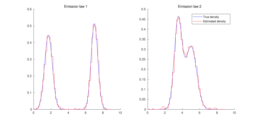
(a) Estimation results for Example 1

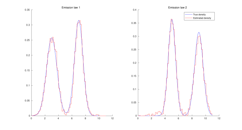
(b) Estimation results for Example 2

Figure 2: Non-parametric penalized least squares density estimation using the histogram basis for Example 1 and Example 2

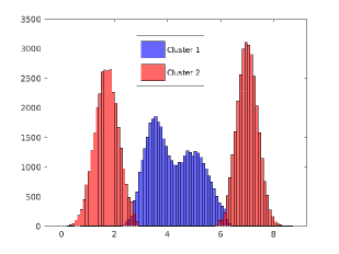
(a) Clustering using plugin clusterer

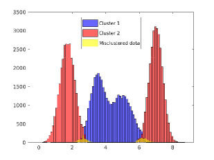
(b) Misclustered observations for plugin clusterer

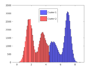
(c) Clustering using $k$-means

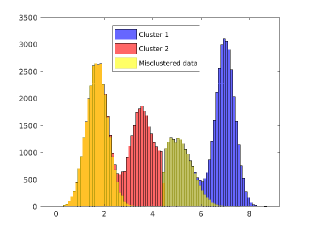
(d) Misclustered observations for $k$-means

Figure 3: Histograms of clusters and clustering errors for Example 1

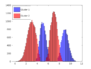
(a) Clustering using plugin clusterer

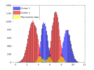
(b) Misclustered observations for plugin clusterer

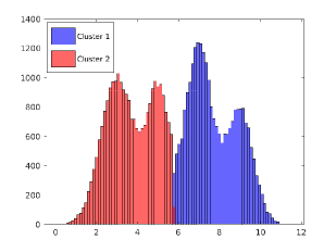
(c) Clustering using $k$-means

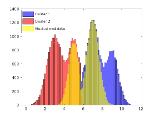
(d) Misclustered observations for $k$-means

Figure 4: Histograms of clusters and clustering errors for Example 2

If the observations were independent and the emissions modelled non-parametrically, the unique quantity that could have been estimated consistently would be the stationary distribution. However, under the HMM assumption, the estimation of each emission density with the minimax rate is possible. This is due to the identifiability of the model which holds even if the emission densities were not constrained to belong to any specific family. This is not possible in the independent case. Figure 2 shows the estimation results of the emission densities and confirms the theoretical properties of the estimator. On the other hand, Theorem 2 proves that in the case of a HMM with two classes, classification errors (and by Theorem 3 clustering error also) could appear only in zones where the two emission densities overlap. In Figures 3(b), and 4(b), misclustered observations appear only in the overlaps between the emission densities.Compared to the $k$-means algorithm which is purely geometric and does not exploit the distribution of the observations, the plugin procedure allows combining together observations even if they are geometrically distant from each other, which is not possible with the $k$-means algorithm. In this context of Gaussian mixtures, the performance of the $k$-means algorithm is mediocre as depicted in Table 1 and does not improve significantly when the overlap between the emission densities is small. However, for the plugin procedure, the more separated are the emission densities, the better are the results of clustering. Note that the results of clustering remain the same whether the observations are clustered online or offline.

5 Discussions and Perspectives

This work focuses on an in-depth study of Bayes risk of clustering. This analysis has led us to prove a form of equivalence between the risk of clustering and the risk of classification. After identifying the key quantity which measures the difficulty of the classification task, it was extrapolated to the Bayes risk of clustering in several regimes. Finally, the excess risk of the plugin procedure was studied. Although the analysis is sufficiently detailed to ensure a thorough understanding of risk of clustering, there are still some interesting questions which were not covered by this work. We give a small overview below.

Lower-bound on entries of $Q$

Throughout our analysis of the Bayes risk of clustering, we have used Assumption 1 which was crucial in obtaining the lower-bounds. In the absence of such an assumption, the lower-bound of Theorem 3 no more matches the upper-bound and the magnitude of the Bayes risk of classification cannot be precisely understood. The same thing applies to the Bayes risk of clustering. In addition, the optimality of the plugin procedure is no more guaranteed.

Approaching the frontier to independence

This situation happens when the emission distributions are nearly similar or when the transition matrix has almost equal lines. In this case, one can hope to improve the coefficient $\frac{\delta}{1-(J-1)\delta}$ which links the Bayes risk of online and offline classification (Theorem 3). In fact, in this situation, the dependence between the observations is so weak and the effect of future observations on the current classification rule is so negligible that the magnitude of the Bayes risk of classification is the same whether in online or offline frameworks. On the other hand, as shown in [2], estimation of the model parameters no more becomes possible when approaching the frontier. The plugin procedure should not work as well.

Lower bounds on the Bayes risk of clustering when it is very small

Theorems 1 and 2 establish lower bounds on the Bayes risk of clustering in term of the Bayes risk of classification. When $J=2$ these bounds are meaningful regardless of how small is the Bayes risk of clustering. When $J=3$, however, these bounds can be vacuous if the Bayes risk of classification gets too small. This is not an artifact of our bounds since we have shown in Proposition 1 that the two Bayes risks are not uniformly comparable when $J\geq 3$. Whence from the current work we only know that the Bayes risk of clustering is driven by $\Lambda$ in the region of parameters for which it is not exponentially small in $n$ and that it cannot be driven by $\Lambda$ otherwise. If it was the case, then it would be equivalent to the Bayes risk of classification in contradiction with the Proposition 1. Understanding the the Bayes risk of clustering in the region of extreme parameters is still an open question.

High dimension

The results concerning the excess risk of the plugin procedure (Corollary 1 and Corollary 2) no more hold in high dimension, that is when the dimension of the observations grows with $n$. The reason is that the estimators of the HMM parameters are not guaranteed to work in high dimension and the constants appearing in the control of the errors of estimation may blow up. However, the other results still apply in this context. Notably, the relationship between classification and clustering risks remains unaffected by observation space dimensionality (Theorem 1 and Theorem 2). Furthermore, the Bayes risk of classification is driven by the same measure of separation $\Lambda$ regardless of the dimension of the observations (Theorem 3).

Fast rates

Corollary 2 has interest mainly in the situation where $\inf_{g\in\mathcal{G}_{n}}\mathcal{R}_{n}^{\mathrm{clust}}(\theta,g)\gtrsim(\log(n)/n)^{\frac{s}{2s+1}}$. In this regime, Corollary 2 tells us that the plugin procedure has a risk of the same magnitude. However, in the situation where the magnitude of the Bayes risk of clustering is much smaller, that is when the emission distributions are very separated, one can hope to obtain faster rates. For example, when $\inf_{g\in\mathcal{G}_{n}}\mathcal{R}_{n}^{\mathrm{clust}}(\theta,g)=\mathcal{O}\left(e^{-cn}\right)$ for $c$ a positive absolute constant, one can hope to show that the risk of the plugin procedure is exponentially small in $n$. The following lemma represents a first step for the proof of such a result.

Lemma 1.

For all $0<\gamma<1/2$ and all $\theta\in\Theta$

$$\mathcal{R}_{n}^{\mathrm{class}}(\theta,\hat{h})\leq\frac{\inf_{h\in\mathcal{H}_{n}}\mathcal{R}_{n}^{\mathrm{class}}(\theta,h)}{1/2-\gamma}+\frac{1}{n}\sum_{i=1}^{n}\mathbb{P}_{\theta}\left(\left\|\phi_{\theta,i\mid n}-\phi_{\hat{\theta},i\mid n}\right\|_{\mathrm{TV}}>\gamma\right).$$ (9)

where $\hat{h}$ is the plugin classifier defined in Section 3.4.

The proof of Lemma 1 is given in Section 6.7.

Observe that the second term of the rhs of (9) is a large deviation term which may eventually decrease exponentially fast in $n$. The only price to pay to obtain large deviation type of decay is a constant factor of at least 2 in front of $\inf_{h\in\mathcal{H}_{n}}\mathcal{R}_{n}^{\mathrm{class}}(\theta,h)$. In situations where $\inf_{h\in\mathcal{H}_{n}}\mathcal{R}_{n}^{\mathrm{class}}(\theta,h)$ is small, this might be advantageous compared to the bound in Corollary 1. Allegedly, the inequality (16) can be used to control the second term in the rhs of (9). This would require to derive large deviation inequalities for all the terms involved in (16), which turns out to be a rather challenging problem.

Optimal excess risk

Although we obtain upper bounds on the excess risk of the plugin procedure (Corollaries 1 and 2), we do not know the optimal rate of decay of the excess risk. In particular, it is unknown if the plugin procedure achieves optimal excess risk. The Lemma 1 suggests that when the Bayes risk is smaller than $\mathcal{O}(n^{-s/(2s+1)})$ then our upper bounds on the excess risk of the plugin could be improved. Yet without optimality guarantees. Determining the optimal excess risk is an open and interesting question to investigate.

Alternatives to plugin

Under the hidden Markov modeling, the most straightforward way to take advantage of the identifiability of the model is to estimate the model parameters and use them for clustering through the plugin procedure. Unlike the i.i.d. case where algorithms such as $k$-means can be used as an alternative, we do not know of any alternative to the plugin in the HMM case. It would be nice to find clustering procedures that leverage the nonparametric identifiability of HMM without relying on estimating the parameters first.

6 Proofs

6.1 Preliminaries

In this section we shall recall basic results for HMMs that can be found in [7] about the distribution of the hidden states given a set of observations.

For any parameter $\theta$, any integers $k$, $i\leq j$, the distribution of $X_{k}$ given $Y_{i:j}$ under $\mathbf{\mathbb{P}}_{\theta}$ will be denoted $\phi_{\theta,k|i:j}(.,Y_{i:j})$. For any integers $i\leq n$, we shall simplify the so-called filtering distribution $\phi_{\theta,n|i:n}(.,Y_{i:n})$ to $\phi_{\theta,n}(.,Y_{i:n})$.

Conditional on observations $Y_{i:n}$, the sequence of the hidden states is an inhomogeneous Markov chain, with transition matrices called forward kernels. For each $k\leq n-1$, the forward kernel is denoted $(F_{\theta,k|n}[Y_{k+1:n}])$ to emphasize that it only depends on $Y_{k+1:n}$. When $k\geq n$, the kernel does not depend on the observations and is equal to the transition matrix $Q$, so that $F_{\theta,k|n}[Y_{k+1:n}]:=Q$ for $k\geq n$. In other words, for any $n\in\mathbf{\mathbb{Z}}$, for any index $i\leq n$ and $k\geq i$ and any real-valued function $f$ on $\mathbb{X}$ (understood as a vector in $\mathbb{R}^{J}$),

$$\mathbf{\mathbb{E}}_{\theta}[f(X_{k+1})\mid X_{i:k},Y_{i:n}]=F_{\theta,k|n}[Y_{k+1:n}]f=\sum_{x\in\mathbb{X}}F_{\theta,k|n}[Y_{k+1:n}](X_{k},x)f(x).$$

Conditional on observations $Y_{i:n}$, the reverse time sequence of hidden states is also an inhomogeneous Markov chain with transition matrices $(B_{\theta,k}[Y_{i:k}])_{k\leq n-1}$ called backward kernels. In other words, for any $n\in\mathbf{\mathbb{Z}}$, $i\leq k\leq n-1$ and any function $f$ on $\mathbb{X}$:

$$\mathbf{\mathbb{E}}_{\theta}[f(X_{k})\mid X_{k+1:n},Y_{i:n}]=B_{\theta,k}[Y_{i:k}]f=\sum_{x\in\mathbb{X}}B_{\theta,k}[Y_{i:k}](X_{k+1},x)f(x).$$

Here, the backward kernel $B_{\theta,k}[Y_{i:k}]$ depends only on the observations up to time $k$. It is given by:

$$B_{\theta,k}[Y_{i:k}](\tilde{x},x)=\frac{\phi_{\theta,k}(x,Y_{i:k})Q(x,\tilde{x})}{\sum_{x^{\prime}\in\mathbb{X}}\phi_{\theta,k}(x^{\prime},Y_{i:k})Q(x^{\prime},\tilde{x})}.$$ (10)

Note that the denominator is always positive thanks to Assumption 1.

For any transition kernel $T$, we denote $\delta(T)$ is the Dobrushin coefficient of $T$ defined by:

$$\begin{split}\delta(T)&=\sup_{(x,x^{\prime})\in\mathbb{X}\times\mathbb{X}}\lVert T(x,.)-T(x^{\prime},.)\rVert_{\mathrm{TV}}\end{split}$$

where $\|\cdot\|_{\mathrm{TV}}$ is the total variation norm. We recall the following two lemmas which can be found in [7].

Lemma 2.

Let $f$ be a real-valued function over $(\mathbb{X},\mathcal{P}(\mathbb{X}))$. Let $\xi$ and $\xi^{\prime}$ be two probability measures over $(\mathbb{X},\mathcal{P}(\mathbb{X}))$ and let $T$ be a transition kernel from $(\mathbb{X},\mathcal{P}(\mathbb{X}))$ to $(\mathbb{Y},\mathcal{Y})$. Then one has:

• $|\xi f-\xi^{\prime}f|\leq\lVert\xi-\xi^{\prime}\rVert_{\mathrm{TV}}osc(f)$
  

• $\lVert\xi T-\xi^{\prime}T\rVert_{TV}\leq\delta(T)\lVert\xi-\xi^{\prime}\rVert_{\mathrm{TV}}$

where $osc(f)=\sup_{(x,x^{\prime})\in\mathbb{X}\times\mathbb{X}}|f(x)-f(x^{\prime})|$.

To end with, notice that under Assumption 1, for any subset $A$ of $\mathbb{X}$,

$$J\delta\gamma(A)\leq\sum_{x^{\prime}\in A}Q(x,x^{\prime})\leq J(1-(J-1)\delta)\gamma(A)$$

with $\gamma$ the uniform distribution over $\mathbb{X}$. Using Lemma 4.3.13 in [7], this leads to

Lemma 3.

Under Assumption 1, for any (possibly non positive) integers $k$ and $n$, the Dobrushin coefficient of the forward kernel $F_{\theta,k|n}$ satisfies:

$$\delta(F_{\theta,k|n})\leq\begin{cases}\rho_{0}&\quad k<n\\ \rho_{1}&\quad k\geq n\end{cases}$$

with $\rho_{0}=1-\frac{J\delta}{J(1-(J-1)\delta)}=\frac{1-J\delta}{1-(J-1)\delta}$ and $\rho_{1}=1-J\delta$.

Using Equation (10) we get that, under Assumption 1, for any (possibly non positive) integers $i\leq k$,

$$\forall x\in\mathbb{X},\qquad B_{\theta,k}[Y_{i:k}](x,.)\geq\frac{\delta}{1-(J-1)\delta}\phi_{\theta,k}(.,Y_{i:k}),$$

so that using applying Lemma 4.3.13 in [7],

Lemma 4.

Under Assumption 1, for any (possibly non positive) integers $i\leq k\leq n-1$, the Dobrushin coefficient of the backward kernel $B_{\theta,k}[Y_{i:k}]$ satisfies:

$$\delta(B_{\theta,k}[Y_{i:k}])\leq 1-\frac{\delta}{1-(J-1)\delta}=\rho_{0}.$$

6.2 Proofs of Theorems 1 and 2

The proofs of Theorems 1 and 2 in the online framework follow the exact same lines of those in the offline case without any change. In addition, the constants appearing in the bounds remain unchanged. We will therefore only present the proofs of the results in the offline framework.

6.2.1 Common elements to the proof of Theorems 1 and 2

Recall the definition of $\mathcal{R}_{n}^{\mathrm{MRSS}}$ in Remark 2: for all $(\theta,h)\in\Theta\times\mathcal{H}_{n}$,

$$\mathcal{R}_{n}^{\mathrm{MRSS}}(\theta,h)=\mathbf{\mathbb{E}}_{\theta}\Big{[}\min_{\tau\in\mathcal{S}_{J}}\mathbf{\mathbb{E}}_{\theta}\big{(}U_{n,\tau}(h)\mid Y_{1:n}\big{)}\Big{]}.$$ (11)

where $U_{n,\tau}(h)\coloneqq\frac{1}{n}\sum_{i=1}^{n}\mathbf{1}_{\tau(X_{i})\neq h_{i}(Y_{1:n})}$.

Instead of comparing $\mathcal{R}_{n}^{\mathrm{clust}}$ and $\mathcal{R}_{n}^{\mathrm{class}}$, we compare $\mathcal{R}_{n}^{\mathrm{clust}}$ and $\mathcal{R}_{n}^{\mathrm{MRSS}}$, which is enough to obtain the result thanks to the following easy lemma.

Lemma 5.

For all $\theta\in\Theta$ and all $n\geq 1$

$$\inf_{h\in\mathcal{H}_{n}}\mathcal{R}_{n}^{\mathrm{class}}(\theta,h)=\inf_{h\in\mathcal{H}_{n}}\mathcal{R}_{n}^{\mathrm{MRSS}}(\theta,h).$$

Proof.

The optimal permutation $\hat{\tau}$ such that $\hat{p}_{\hat{\tau}}(h)=\min_{\tau\in\mathcal{S}_{J}}\mathbf{\mathbb{E}}_{\theta}(U_{n,\tau}(h)\mid Y_{1:n})$ is a $Y_{1:n}$-measurable permutation valued random variable. Since any $h\in\mathcal{H}_{n}$ is also $Y_{1:n}$-measurable, the result is immediate. ∎

In the next we then focus on comparing $\mathcal{R}_{n}^{\mathrm{clust}}$ and $\mathcal{R}_{n}^{\mathrm{MRSS}}$. We let $N_{j}\coloneqq\sum_{i=1}^{n}\mathbf{1}_{\{X_{i}=j\}}$ and $N_{(1)}\leq N_{(2)}\leq\dots\leq N_{(J)}$ denote the order statistics of $(N_{1},\dots,N_{J})$. We also make use of the notation $\hat{p}_{\tau}(h)\coloneqq\mathbf{\mathbb{E}}_{\theta}(U_{n,\tau}(h)\mid Y_{1:n})$. We also let $\hat{\tau}_{h}$ denote a $Y_{1:n}$-measurable permutation satisfying:

$$\hat{p}_{\hat{\tau}_{h}}(h)=\mathbf{\mathbb{E}}_{\theta}(U_{n,\hat{\tau}_{h}}(h)\mid Y_{1:n})=\min_{\tau}\mathbf{\mathbb{E}}_{\theta}(U_{n,\tau}(h)\mid Y_{1:n})=\min_{\tau}\hat{p}_{\tau}(h).$$

Proposition 2.

A generic lower bound that works for any latent model (i.i.d. or HMM or whatever). For all classifiers $h$, all $\varepsilon$ and all $\eta$

$$\mathbf{\mathbb{E}}_{\theta}\Big{(}\min_{\tau}U_{n,\tau}(h)\Big{)} \geq\mathbf{\mathbb{E}}_{\theta}\Big{(}\min_{\tau}\mathbf{\mathbb{E}}_{\theta}(U_{n,\tau}(h)\mid Y_{1:n})\Big{)}$$

$$\quad-\mathbf{\mathbb{E}}_{\theta}\Big{(}\mathbf{\mathbb{E}}_{\theta}\Big{(}\max_{\tau}[-U_{n,\tau}(h)+\hat{p}_{\tau}(h)]\mid Y_{1:n}\Big{)}\mathbf{1}_{\{\hat{p}_{\hat{\tau}_{h}}(h)\geq\varepsilon\}}\Big{)}$$

$$\quad-\mathbf{\mathbb{E}}_{\theta}\Big{(}\mathbf{\mathbb{P}}_{\theta}(U_{n,\hat{\tau}_{h}}(h)>\eta\mid Y_{1:n})\mathbf{1}_{\{\hat{p}_{\hat{\tau}_{h}}(h)<\varepsilon\}}\Big{)}$$

$$\quad-\mathbf{\mathbb{P}}_{\theta}\big{(}N_{(1)}+N_{(2)}<2n\eta\big{)}.$$

Proof.

For $\varepsilon\in[0,1]$, we decompose

$$\mathbf{\mathbb{E}}_{\theta}\Big{(}\min_{\tau}U_{n,\tau}(h)\Big{)}=\mathbf{\mathbb{E}}_{\theta}\Big{(}\min_{\tau}U_{n,\tau}(h)\mathbf{1}_{\{\hat{p}_{\hat{\tau}_{h}}(h)\geq\varepsilon\}}\Big{)}+\mathbf{\mathbb{E}}_{\theta}\Big{(}\min_{\tau}U_{n,\tau}(h)\mathbf{1}_{\{\hat{p}_{\hat{\tau}_{h}}(h)<\varepsilon\}}\Big{)}.$$ (12)

The first term in the rhs of (12) is handled via a small deviation principle, remarking that on the event $\{\hat{p}_{\hat{\tau}(h)}(h)\geq\varepsilon\}$

$$\mathbf{\mathbb{E}}_{\theta}\Big{(}\min_{\tau}U_{n,\tau}(h)\mid Y_{1:n}\Big{)} =\mathbf{\mathbb{E}}_{\theta}\Big{(}\min_{\tau}[\hat{p}_{\tau}(h)+U_{n,\tau}(h)-\hat{p}_{\tau}(h)]\mid Y_{1:n}\Big{)}$$

$$\geq\min_{\tau}\hat{p}_{\tau}(h)-\mathbf{\mathbb{E}}_{\theta}\Big{(}\max_{\tau}[-U_{n,\tau}(h)+\hat{p}_{\tau}(h)]\mid Y_{1:n}\Big{)}.$$

The second term in (12) is handled via a large deviation principle. By Lemma 6, on the event $\{\hat{p}_{\hat{\tau}_{h}}(h)<\varepsilon\}$

$$\mathbf{\mathbb{E}}_{\theta}\Big{(}\min_{\tau}U_{n,\tau}(h)\mid Y_{1:n}\Big{)} \geq\mathbf{\mathbb{E}}_{\theta}\Big{(}\min_{\tau}U_{n,\tau}(h)\mathbf{1}_{\{U_{n,\hat{\tau}_{h}}(h)\leq(N_{(1)}+N_{(2)})/(2n)\}}\mid Y_{1:n}\Big{)}$$

$$=\mathbf{\mathbb{E}}_{\theta}\Big{(}U_{n,\hat{\tau}_{h}}(h)\mathbf{1}_{\{U_{n,\hat{\tau}_{h}}(h)\leq(N_{(1)}+N_{(2)})/(2n)\}}\mid Y_{1:n}\Big{)}$$

$$\geq\hat{p}_{\hat{\tau}_{h}}(h)-\mathbf{\mathbb{P}}_{\theta}\Big{(}U_{n,\hat{\tau}_{h}}(h)>\frac{N_{(1)}+N_{(2)}}{2n}\mid Y_{1:n}\Big{)}.$$

But,

$$\mathbf{\mathbb{P}}_{\theta}\Big{(}U_{n,\hat{\tau}_{h}}(h)>\frac{N_{(1)}+N_{(2)}}{2n}\mid Y_{1:n}\Big{)} \leq\mathbf{\mathbb{P}}_{\theta}\big{(}U_{n,\hat{\tau}_{h}}>\eta\mid Y_{1:n}\big{)}+\mathbf{\mathbb{P}}_{\theta}\big{(}N_{(1)}+N_{(2)}<2n\eta\mid Y_{1:n}\big{)}.$$

The generic lower bound follows. ∎

Lemma 6.

If $U_{n,\tau^{\prime}}(h)\leq\frac{N_{(1)}+N_{(2)}}{2n}$ then $\min_{\tau}U_{n,\tau}(h)=U_{n,\tau^{\prime}}(h)$.

Proof.

Let $U_{n,\tau^{\prime}}(h)\leq\frac{N_{(1)}+N_{(2)}}{2n}$ and suppose $\min_{\tau}U_{n,\tau}(h)<U_{n,\tau^{\prime}}(h)$. Then, there exists a permutation $\tau^{\prime\prime}\neq\tau^{\prime}$ such that $U_{n,\tau^{\prime\prime}}(h)<U_{n,\tau^{\prime}}(h)$. But then, letting $I=\{i\in\{1,\dots,n\}\;:\;\tau^{\prime}(X_{i})=h_{i}(Y_{1:n})\}$:

$$n(U_{n,\tau^{\prime}}(h)-U_{n,\tau^{\prime\prime}}(h)) =\sum_{i=1}^{n}\Big{(}\mathbf{1}_{\{\tau^{\prime}(X_{i})\neq h_{i}(Y_{1:n})\}}-\mathbf{1}_{\{\tau^{\prime\prime}(X_{i})\neq h_{i}(Y_{1:n})\}}\Big{)}$$

$$=\sum_{i=1}^{n}\Big{(}\mathbf{1}_{\{\tau^{\prime\prime}(X_{i})=h_{i}(Y_{1:n})\}}-\mathbf{1}_{\{\tau^{\prime}(X_{i})=h_{i}(Y_{1:n})\}}\Big{)}$$

$$=-\sum_{i\in I}\mathbf{1}_{\{\tau^{\prime}(X_{i})\neq\tau^{\prime\prime}(X_{i})\}}+\sum_{i\in I^{c}}\mathbf{1}_{\{\tau^{\prime}(X_{i})=h_{i}(Y_{1:n})\}}$$

$$=-\sum_{i=1}^{n}\mathbf{1}_{\{\tau^{\prime}(X_{i})\neq\tau^{\prime\prime}(X_{i})\}}+\sum_{i\in I^{c}}\Big{(}\mathbf{1}_{\{\tau^{\prime}(X_{i})=h_{i}(Y_{1:n})\}}+\mathbf{1}_{\{\tau^{\prime}(X_{i})\neq\tau^{\prime\prime}(X_{i})\}}\Big{)}$$

$$\leq-(N_{(1)}+N_{(2)})+2|I^{c}|$$

$$=-(N_{(1)}+N_{(2)})+2nU_{n,\tau^{\prime}}(h)$$

where we have used that since $\tau^{\prime}\neq\tau^{\prime\prime}$, it must be that $\sum_{i=1}^{n}\mathbf{1}_{\tau^{\prime}(X_{i})\neq\tau^{\prime\prime}(X_{i})}\geq N_{(1)}+N_{(2)}$. Rearranging the previous:

$$U_{n,\tau^{\prime\prime}}(h)\geq\frac{N_{(1)}+N_{(2)}}{n}-U_{n,\tau^{\prime}}(h)\geq U_{n,\tau^{\prime}}(h).$$

which contradicts that $U_{n,\tau^{\prime\prime}}(h)<U_{n,\tau^{\prime}}(h)$. Hence $\min_{\tau}U_{n,\tau}(h)\geq U_{n,\tau^{\prime}}(h)$. ∎

6.2.2 Proof of Theorem 1 (independent scenario)

Here we apply the result of Proposition 2 to the i.i.d. case. The first trivial bound is obtained by choosing $\varepsilon=\eta=0$. With this choice, Proposition 2 gives

$$\mathbf{\mathbb{E}}_{\theta}\Big{(}\min_{\tau}U_{n,\tau}(h)\Big{)} \geq\mathbf{\mathbb{E}}_{\theta}\Big{(}\min_{\tau}\mathbf{\mathbb{E}}_{\theta}(U_{n,\tau}(h)\mid Y_{1:n})\Big{)}-\mathbf{\mathbb{E}}_{\theta}\Big{(}\mathbf{\mathbb{E}}_{\theta}\Big{(}\max_{\tau}[-U_{n,\tau}(h)+\hat{p}_{\tau}(h)]\mid Y_{1:n}\Big{)}\Big{)}$$

$$\geq\mathbf{\mathbb{E}}_{\theta}\Big{(}\min_{\tau}\mathbf{\mathbb{E}}_{\theta}(U_{n,\tau}(h)\mid Y_{1:n})\Big{)}-\sqrt{\frac{\log(J!)}{2n}}$$

by Lemma 7 below. The other bounds are obtained using Lemma 7 and Markov’s inequality to establish that for any $\varepsilon>0$

$$\mathbf{\mathbb{E}}_{\theta}\Big{(}\mathbf{\mathbb{E}}_{\theta}\Big{(}\max_{\tau}[-U_{n,\tau}(h)+\hat{p}_{\tau}(h)]\mid Y_{1:n}\Big{)}\mathbf{1}_{\{\hat{p}_{\hat{\tau}_{h}}(h)\geq\varepsilon\}}\Big{)}\\ \begin{aligned} &\leq\sqrt{\frac{\log(J!)}{2n}}\mathbf{\mathbb{P}}_{\theta}\big{(}\hat{p}_{\hat{\tau}_{h}}(h)\geq\varepsilon\big{)}\\ &\leq\frac{1}{\varepsilon}\sqrt{\frac{\log(J!)}{2n}}\mathbf{\mathbb{E}}_{\theta}\Big{(}\min_{\tau}\mathbf{\mathbb{E}}_{\theta}(U_{n,\tau}(h)\mid Y_{1:n})\mathbf{1}_{\{\hat{p}_{\hat{\tau}_{h}}(h)\geq\varepsilon\}}\Big{)}\end{aligned}$$

and then using Lemma 8 to establish that for all $\varepsilon,\eta>0$

$$\mathbf{\mathbb{E}}_{\theta}\Big{(}\mathbf{\mathbb{P}}_{\theta}(U_{n,\hat{\tau}_{h}}(h)>\eta\mid Y_{1:n})\mathbf{1}_{\{\hat{p}_{\hat{\tau}_{h}}(h)<\varepsilon\}}\Big{)} \leq\mathbf{\mathbb{E}}_{\theta}\Big{(}\hat{p}_{\hat{\tau}_{h}}(h)\cdot\frac{e}{\eta}\Big{(}\frac{e\hat{p}_{\hat{\tau}_{h}}(h)}{\eta}\Big{)}^{n\eta-1}e^{-n\hat{p}_{\hat{\tau}_{h}}(h)}\mathbf{1}_{\{\hat{p}_{\hat{\tau}_{h}}(h)<\varepsilon\}}\Big{)}$$

$$\leq\frac{e}{\eta}\Big{(}\frac{e\varepsilon}{\eta}\Big{)}^{n\eta-1}\mathbf{\mathbb{E}}_{\theta}\Big{(}\min_{\tau}\mathbf{\mathbb{E}}_{\theta}(U_{n,\tau}(h)\mid Y_{1:n})\mathbf{1}_{\{\hat{p}_{\hat{\tau}_{h}}(h)<\varepsilon\}}\Big{)}.$$

From here, observe that when $J=2$ it must be that $\mathbf{\mathbb{P}}_{\theta}(N_{(1)}+N_{(2)}<n)=0$. Then, the bound in this case follows by taking $\eta\to\frac{1}{2}$ [by below] and $\varepsilon=\frac{1}{2e}[\log(J!)/(2n)]^{1/n}$.

When $J\geq 3$, Lemma 9 can be used to find that

$$\mathbf{\mathbb{P}}_{\theta}\big{(}N_{(1)}+N_{(2)}<2n\eta\big{)}\leq J^{2}e^{-\frac{n(\beta-2\eta)^{2}}{2\beta}}.$$

Then the remaining bound is obtained by choosing $\eta=\beta/4$ and $\varepsilon=\frac{\beta}{4e}[\log(J!)/(2n)]^{2/(n\beta)}$.

Lemma 7.

For all $\theta$, $\mathbf{\mathbb{P}}_{\theta}$-almost-surely

$$\mathbf{\mathbb{E}}_{\theta}\Big{(}\max_{\tau}[-U_{n,\tau}(h)+\hat{p}_{\tau}(h)]\mid Y_{1:n}\Big{)}\leq\sqrt{\frac{\log(J!)}{2n}}.$$

Proof.

For any $\lambda>0$,

$$\begin{split}\mathbf{\mathbb{E}}_{\theta}\left[\sup_{\tau}\left\{-U_{n,\tau}(h)+\hat{p}_{\tau}(h)\right\}\right]&\leq\frac{1}{\lambda}\log\left(\mathbf{\mathbb{E}}_{\theta}\left[\exp\left(\sup_{\tau}\left\{-\lambda\left(U_{n,\tau}(h)-\hat{p}_{\tau}(h)\right)\right\}\right)\bigg{|}Y_{1:n}\right]\right)\\ &=\frac{1}{\lambda}\log\left(\mathbf{\mathbb{E}}_{\theta}\left[\sup_{\tau}\exp\left(-\lambda\left(U_{n,\tau}(h)-\hat{p}_{\tau}(h)\right)\right)\bigg{|}Y_{1:n}\right]\right)\\ &\leq\frac{1}{\lambda}\log\left(J!\sup_{\tau}\mathbf{\mathbb{E}}_{\theta}\left[\exp\left(-\lambda\left(U_{n,\tau}(h)-\hat{p}_{\tau}(h)\right)\right)\bigg{|}Y_{1:n}\right]\right)\\ &\leq\frac{1}{\lambda}\log\left(J!\exp\left(\frac{\lambda^{2}}{8}\times n\times\left(\frac{1}{n}\right)^{2}\right)\right)\text{(Hoeffding's lemma)}\\ &\leq\inf_{\lambda>0}\left\{\frac{\log(J!)}{\lambda}+\frac{\lambda}{8n}\right\}\\ &\leq\sqrt{\frac{\log(J!)}{2n}}.\end{split}$$

Hoeffding’s lemma applies because conditionally to the sequence of observations $Y_{1:n}$, the labels $X_{1:n}$ are still independent. ∎

Lemma 8.

For all $\theta\in\Theta$, $\mathbf{\mathbb{P}}_{\theta}$-almost-surely

$$\mathbf{\mathbb{P}}_{\theta}\big{(}U_{n,\hat{\tau}_{h}}(h)>\eta\mid Y_{1:n}\big{)}\leq\hat{p}_{\hat{\tau}_{h}}(h)\cdot\frac{e}{\eta}\Big{(}\frac{e\hat{p}_{\hat{\tau}_{h}}(h)}{\eta}\Big{)}^{n\eta-1}e^{-n\hat{p}_{\hat{\tau}_{h}}(h)}.$$

Proof.

By Chernoff’s bound [with $q_{i}(h)=\mathbf{\mathbb{P}}_{\theta}(h_{i}(Y_{1:n})\neq\hat{\tau}_{h}(X_{i})\mid Y_{1:n})$]:

$$\mathbf{\mathbb{P}}_{\theta}\big{(}U_{n,\hat{\tau}_{h}}(h)>\eta\mid Y_{1:n}\big{)} =\mathbf{\mathbb{P}}_{\theta}\Big{(}\sum_{i=1}^{n}\mathbf{1}_{h_{i}(Y_{1:n})\neq\hat{\tau}_{h}(X_{i})}>n\eta\mid Y_{1:n}\Big{)}$$

$$\leq\inf_{\lambda>0}\exp\Big{(}-\lambda n\eta+\sum_{i=1}^{n}\log\Big{(}q_{i}(h)e^{\lambda}+1-q_{i}(h)\Big{)}\Big{)}$$

$$\leq\inf_{\lambda>0}\exp\Big{(}-\lambda n\eta+n\hat{p}_{\hat{\tau}_{h}}(h)(e^{\lambda}-1)\Big{)}$$

$$=\Big{(}\frac{e\hat{p}_{\hat{\tau}_{h}}(h)}{\eta}\Big{)}^{n\eta}e^{-n\hat{p}_{\hat{\tau}_{h}}(h)}$$

$$\leq\hat{p}_{\hat{\tau}_{h}}(h)\cdot\frac{e}{\eta}\Big{(}\frac{e\hat{p}_{\hat{\tau}_{h}}(h)}{\eta}\Big{)}^{n\eta-1}e^{-n\hat{p}_{\hat{\tau}_{h}}(h)}.$$

∎

Lemma 9.

Let $\beta=\min_{j\neq k}(\nu_{j}+\nu_{k})$. If $J\geq 3$, then

$$\mathbf{\mathbb{P}}_{\theta}\big{(}N_{(1)}+N_{(2)}<2n\eta\big{)}\leq J^{2}e^{-\frac{n(\beta-2\eta)^{2}}{2\beta}}.$$

Proof.

If $J=2$, remark that $N_{(1)}+N_{(2)}=n$ $P_{\theta}$-almost-surely, hence the result. Now we assume that $J\geq 3$. It holds,

$$\mathbf{\mathbb{P}}_{\theta}\big{(}N_{(1)}+N_{(2)}<2n\eta\big{)} =P_{\theta}\big{(}\exists\,j\neq k,\ N_{j}+N_{k}\leq 2n\eta\big{)}$$

$$\leq J^{2}\max_{j\neq k}\mathbf{\mathbb{P}}_{\theta}\big{(}N_{j}+N_{k}\leq 2n\eta\big{)}.$$

Then observe that $N_{j}+N_{k}=\sum_{i=1}^{n}(\mathbf{1}_{X_{i}=j}+\mathbf{1}_{X_{i}=k})=\sum_{i=1}^{n}\mathbf{1}_{X_{i}\in\{j,k\}}$ whenever $j\neq k$. In other words, when $j\neq k$ the random variables $N_{j}+N_{k}$ has a Binomial distribution with parameters $(n,\nu_{j}+\nu_{k})$ under $\mathbf{\mathbb{P}}_{\theta}$. The conclusion follows using Chernoff’s bound on the Binomial distribution [recall the Binomial distribution is sub-Gaussian on the left-tail]. ∎

6.2.3 Proof of Theorem 2 (dependent scenario)

We apply the result of Proposition 2 to the HMM case. The first trivial bound is obtained by choosing $\varepsilon=\delta=0$. Proposition 2 yields:

$$\mathbf{\mathbb{E}}_{\theta}\Big{(}\min_{\tau}U_{n,\tau}(h)\Big{)} \geq\mathbf{\mathbb{E}}_{\theta}\Big{(}\min_{\tau}\mathbf{\mathbb{E}}_{\theta}(U_{n,\tau}(h)\mid Y_{1:n})\Big{)}-\mathbf{\mathbb{E}}_{\theta}\Big{(}\mathbf{\mathbb{E}}_{\theta}\Big{(}\max_{\tau}[\hat{p}_{\tau}(h)-U_{n,\tau}(h)]\mid Y_{1:n}\Big{)}\Big{)}$$

$$\geq\mathbf{\mathbb{E}}_{\theta}\Big{(}\min_{\tau}\mathbf{\mathbb{E}}_{\theta}(U_{n,\tau}(h)\mid Y_{1:n})\Big{)}-\frac{1}{1-\rho_{0}}\sqrt{\frac{\log(J!)}{2n}}$$

by Lemma 10 below. The first inequality follows by taking the infimum over h on both sides.

The other bounds are obtained using Lemma 10 and Markov’s inequality as in the independent case:

$$\mathbf{\mathbb{E}}_{\theta}\Big{(}\mathbf{\mathbb{E}}_{\theta}\Big{(}\max_{\tau}[-U_{n,\tau}(h)+\hat{p}_{\tau}(h)]\mid Y_{1:n}\Big{)}\mathbf{1}_{\{\hat{p}_{\hat{\tau}_{h}}(h)\geq\varepsilon\}}\Big{)}\\ \begin{aligned} &\leq\frac{1}{1-\rho_{0}}\sqrt{\frac{\log(J!)}{2n}}\mathbf{\mathbb{P}}_{\theta}\big{(}\hat{p}_{\hat{\tau}_{h}}(h)\geq\varepsilon\big{)}\\ &\leq\frac{1}{\varepsilon(1-\rho_{0})}\sqrt{\frac{\log(J!)}{2n}}\mathbf{\mathbb{E}}_{\theta}\Big{(}\min_{\tau}\mathbf{\mathbb{E}}_{\theta}(U_{n,\tau}(h)\mid Y_{1:n})\mathbf{1}_{\{\hat{p}_{\hat{\tau}_{h}}(h)\geq\varepsilon\}}\Big{)}\end{aligned}$$

and then using Lemma 11 to establish that for all $\varepsilon,\eta>0$

$$\mathbf{\mathbb{E}}_{\theta}\Big{(}\mathbf{\mathbb{P}}_{\theta}(U_{n,\hat{\tau}_{h}}(h)>\eta\mid Y_{1:n})\mathbf{1}_{\{\hat{p}_{\hat{\tau}_{h}}(h)<\varepsilon\}}\Big{)}\\ \begin{aligned} &\leq\mathbf{\mathbb{E}}_{\theta}\Big{(}\hat{p}_{\hat{\tau}_{h}}(h)\cdot\frac{e}{\eta}\left(\frac{1-(J-1)\delta}{\delta}\right)^{2n}\Big{(}\frac{e\hat{p}_{\hat{\tau}_{h}}(h)}{\eta}\Big{)}^{n\eta-1}e^{-n\hat{p}_{\hat{\tau}_{h}}(h)}\mathbf{1}_{\{\hat{p}_{\hat{\tau}_{h}}(h)<\varepsilon\}}\Big{)}\\ &\leq\frac{e}{\eta}\left(\frac{1-(J-1)\delta}{\delta}\right)^{2n}\Big{(}\frac{e\varepsilon}{\eta}\Big{)}^{n\eta-1}\mathbf{\mathbb{E}}_{\theta}\Big{(}\min_{\tau}\mathbf{\mathbb{E}}_{\theta}(U_{n,\tau}(h)\mid Y_{1:n})\mathbf{1}_{\{\hat{p}_{\hat{\tau}_{h}}(h)<\varepsilon\}}\Big{)}.\end{aligned}$$

From here, observe that when $J=2$ it must be that $\mathbf{\mathbb{P}}_{\theta}(N_{(1)}+N_{(2)}<n)=0$. Then, the bound in this case follows by taking $\eta\to\frac{1}{2}$ [by below] and $\varepsilon=\frac{1}{2e}\left(\frac{\delta}{1-\delta}\right)^{4}[\log(J!)/(2n)]^{1/n}$.

For the remaining inequality, when $J\geq 3$, Lemma 12 ensures:

$$\mathbf{\mathbb{P}}_{\theta}\big{(}N_{(1)}+N_{(2)}<2n\eta\big{)}\leq J^{2}e^{-2n(1-\rho_{1})^{2}(\beta-2\eta)^{2}}.$$

On the other hand, we have by Lemma 10:

$$\mathbf{\mathbb{E}}_{\theta}\left[\max_{\tau}\left\{\hat{p}_{\tau}(h)-U_{n,\tau}(h)\right\}\mid Y_{1:n}\right]\leq\frac{1}{1-\rho_{0}}\sqrt{\frac{\log(J!)}{2n}}$$

On the event: $\left\{\hat{p}_{\hat{\tau}_{h}}(h)<\varepsilon\right\}$, for $\varepsilon<\eta$:

$$\begin{split}\mathbf{\mathbb{P}}_{\theta}\left(U_{n,\hat{\tau}_{h}}(h)>\eta\mid Y_{1:n}\right)&=\mathbf{\mathbb{P}}_{\theta}\left(U_{n,\hat{\tau}_{h}}(h)-\hat{p}_{\hat{\tau}_{h}}(h)>\eta-\hat{p}_{\hat{\tau}_{h}}(h)\mid Y_{1:n}\right)\\ &\leq\mathbf{\mathbb{P}}_{\theta}\left(U_{n,\hat{\tau}_{h}}(h)-\hat{p}_{\hat{\tau}_{h}}(h)>\eta-\varepsilon\mid Y_{1:n}\right)\\ &\leq e^{-\lambda(\eta-\varepsilon)}\mathbf{\mathbb{E}}_{\theta}\left[e^{\lambda\left\{U_{n,\hat{\tau}_{h}}(h)-\hat{p}_{\hat{\tau}_{h}}(h)\right\}}\mid Y_{1:n}\right]\\ &\leq e^{-\lambda(\eta-\varepsilon)}e^{\frac{1}{8n}\left(\frac{\lambda}{1-\rho_{0}}\right)^{2}}\end{split}$$

where the last inequality is due to the argument using Marton coupling as shown in the proof of Lemma 10. Taking the minimum over $\lambda$ yields:

$$\mathbf{\mathbb{E}}_{\theta}\left[\mathbf{\mathbb{P}}_{\theta}\left(U_{n,\hat{\tau}_{h}}(h)>\eta\mid Y_{1:n}\right)\mathbf{1}_{\hat{p}_{\hat{\tau}_{h}}(h)<\varepsilon}\right]\leq e^{-2n(1-\rho_{0})^{2}(\eta-\varepsilon)^{2}}$$

Using Lemma 12, the final bound reads:

$$\begin{split}\mathbf{\mathbb{E}}_{\theta}\left[\min_{\tau}U_{n,\tau}(h)\right]&\geq\mathbf{\mathbb{E}}_{\theta}\left[\min_{\tau}\mathbf{\mathbb{E}}_{\theta}\left[U_{n,\tau}(h)\mid Y_{1:n}\right]\right]\\ &-\frac{1}{\varepsilon(1-\rho_{0})}\sqrt{\frac{\log(J!)}{2n}}\mathbf{\mathbb{E}}_{\theta}\left[\hat{p}_{\hat{\tau}_{h}}(h)\mathbf{1}_{\hat{p}_{\hat{\tau}_{h}}(h)\geq\varepsilon}\right]\\ &-e^{-2n(1-\rho_{0})^{2}(\eta-\varepsilon)^{2}}-J^{2}e^{-2n(1-\rho_{1})^{2}(\beta-2\eta)^{2}}\end{split}$$

Choosing $\varepsilon=\frac{\eta}{2}$ and $\eta=\frac{2}{5}\beta$ and noting that $\rho_{1}<\rho_{0}$ one obtains:

$$\mathbf{\mathbb{E}}_{\theta}\left[\min_{\tau}U_{n,\tau}(h)\right] \geq\left[1-\frac{5}{\beta(1-\rho_{0})}\sqrt{\frac{\log(J!)}{2n}}\right]\mathbf{\mathbb{E}}_{\theta}\left[\min_{\tau}\mathbf{\mathbb{E}}_{\theta}\left[U_{n,\tau}(h)\mid Y_{1:n}\right]\right]$$

$$\quad-(J^{2}+1)e^{-cn(1-\rho_{0})^{2}\beta^{2}}.$$

The result follows.

Lemma 10.

Under Assumptions 1 and 2, for all $\theta\in\Theta^{\mathrm{dep}}$, $\mathbf{\mathbb{P}}_{\theta}$-almost-surely

$$\mathbf{\mathbb{E}}_{\theta}\left[\max_{\tau}\left\{\hat{p}_{\tau}(h)-U_{n,\tau}(h)\right\}\mid Y_{1:n}\right]\leq\frac{1}{1-\rho_{0}}\sqrt{\frac{\log(J!)}{2n}}$$

where $\rho_{0}=\frac{1-J\delta}{1-(J-1)\delta}$.

Proof.

Given that for any $\lambda>0$,

$$\mathbf{\mathbb{E}}_{\theta}\left[\max_{\tau}\left\{\hat{p}_{\tau}(h)-(U_{n,\tau}(h)\right\}\right]\leq\frac{1}{\lambda}\log\left(J!\max_{\tau}\mathbf{\mathbb{E}}_{\theta}\left[\exp\left(-\lambda(U_{n,\tau}(h)-\hat{p}_{\tau}(h))\right)\bigg{|}Y_{1:n}\right]\right)$$

we shall exhibit an upper bound of the rhs term by applying Theorem 2.9 of [39], conditional on $Y_{1:n}$. So that for now we consider $Y=Y_{1:n}$ as fixed. Define $f_{Y}^{h,\tau}$ for any $x=x_{1:n}$ by:

$$f_{Y}^{h,\tau}(x)=-\frac{1}{n}\sum_{i=1}^{n}\mathbf{1}_{\tau(x_{i})\neq h_{i}(Y_{1:n})}.$$

Then, for any $x=x_{1:n}$ and $x^{\prime}=x^{\prime}_{1:n}$,

$$f_{Y}^{h,\tau}(x)-f_{Y}^{h,\tau}(x^{\prime})\leq\frac{1}{n}\sum_{i=1}^{n}\mathbf{1}_{x_{i}\neq x_{i}^{\prime}}.$$

We thus may apply (2.5) in Theorem 2.9 of [39] to get

$$\mathbf{\mathbb{E}}_{\theta}\left[e^{\lambda(f_{Y}^{h,\tau}(X)-\mathbf{\mathbb{E}}_{\theta}\left[f_{Y}^{h,\tau}(X)\mid Y_{1:n}\right])}\bigg{|}Y_{1:n}\right]\leq e^{\frac{\lambda^{2}}{8n^{2}}\sum_{i=1}^{n}\left(\sum_{j=i}^{n}\Gamma_{i,j}\right)^{2}},$$ (13)

where $\Gamma$ comes from a Marton coupling (see Definition 2.1 in [39]) and is given by:

$$\Gamma_{j,i}:=0,\qquad\Gamma_{i,j}:=\sup_{x_{1},\ldots,x_{i},x_{i}^{\prime}\in\mathbb{X}}\mathbb{P}_{\theta}\left[X_{1,j}^{\left(x_{1},\ldots,x_{i},x_{i}^{\prime},Y_{1:n}\right)}\neq X_{2,j}^{\left(x_{1},\ldots,x_{i},x_{i}^{\prime},Y_{1:n}\right)}\bigg{|}Y_{1:n}\right]$$

for $1\leq i<j\leq n$. Now,

$$\Gamma_{i,j}\leq\sup_{x_{1:i-1}\in\mathbb{X}^{i-1}}\Bigg{\|}\mathbf{\mathbb{P}}_{\theta}\left(X_{1,j}^{(x_{1:i-1},\tilde{a},\tilde{b},Y_{1:n})}\in\cdot\bigg{|}X_{1:i-1}=x_{1:i-1},Y_{1:n}\right)\\ -\mathbf{\mathbb{P}}_{\theta}\left(X_{2,j}^{(x_{1:i-1},\tilde{a},\tilde{b},Y_{1:n})}\in\cdot\bigg{|}X_{1:i-1}=x_{1:i-1},Y_{1:n}\right)\Bigg{\|}_{\mathrm{TV}},$$

ie.,

$$\Gamma_{i,j}\leq\sup_{x_{1:i-1}\in\mathbb{X}^{i-1}}\Bigg{\|}\mathbf{\mathbb{P}}_{\theta}\left(X_{j}\in\cdot\bigg{|}X_{1:i-1}=x_{1:i-1},X_{i}=\tilde{a},Y_{1:n}\right)\\ -\mathbf{\mathbb{P}}_{\theta}\left(X_{j}\in\cdot\bigg{|}X_{1:i-1}=x_{1:i-1},X_{i}=\tilde{b},Y_{1:n}\right)\Bigg{\|}_{\mathrm{TV}},$$

ie.,

$$\Gamma_{i,j}\leq\Bigg{\|}\mathbf{\mathbb{P}}_{\theta}\left(X_{j}\in\cdot\bigg{|}X_{i}=\tilde{a},Y_{1:n}\right)-\mathbf{\mathbb{P}}_{\theta}\left(X_{j}\in\cdot\bigg{|}X_{i}=\tilde{b},Y_{1:n}\right)\Bigg{\|}_{\mathrm{TV}}$$

since conditional on $Y_{1:n}$, the hidden states form a nonhomogeneous Markov chain with transition kernels $(F_{k|n}[Y_{k+1:n}])$. Exponential forgetting of the smoothing distributions in HMMs (Proposition 4.3.26 in [7]) allows to conclude that

$$\Bigg{\|}\mathbf{\mathbb{P}}_{\theta}\left(X_{j}\in\cdot\bigg{|}X_{i}=\tilde{a},Y_{1:n}\right)-\mathbf{\mathbb{P}}_{\theta}\left(X_{j}\in\cdot\bigg{|}X_{i}=\tilde{b},Y_{1:n}\right)\Bigg{\|}_{\mathrm{TV}}\leq\rho_{0}^{j-i}$$

where $\rho_{0}=\frac{1-J\delta}{1-(J-1)\delta}$ (see also Lemma 3). By inequality (13):

$$\max_{\tau}\mathbf{\mathbb{E}}_{\theta}\left[e^{\lambda(f_{Y}^{h,\tau}(X)-\mathbf{\mathbb{E}}_{\theta}\left[f_{Y}^{h,\tau}(X)\mid Y_{1:n}\right])}\bigg{|}Y_{1:n}\right]\leq e^{\frac{1}{8n}\left(\frac{\lambda}{1-\rho_{0}}\right)^{2}}.$$

Thus,

$$\mathbf{\mathbb{E}}_{\theta}\left[\max_{\tau}\left\{\hat{p}_{\tau}(h)-U_{n,\tau}(h)\right\}\bigg{|}Y_{1:n}\right] \leq \inf_{\lambda>0}\left\{\frac{\log(J!)}{\lambda}+\frac{\lambda}{8n(1-\rho_{0})^{2}}\right\}$$

$$= \frac{1}{1-\rho_{0}}\sqrt{\frac{\log(J!)}{2n}}$$

∎

Lemma 11.

For all $\theta\in\Theta$, $\mathbf{\mathbb{P}}_{\theta}$-almost-surely

$$\mathbf{\mathbb{P}}_{\theta}\big{(}U_{n,\hat{\tau}_{h}}(h)>\eta\mid Y_{1:n}\big{)}\leq\hat{p}_{\hat{\tau}_{h}}(h)\cdot\frac{e}{\eta}\left(\frac{1-(J-1)\delta}{\delta}\right)^{2n}\Big{(}\frac{e\hat{p}_{\hat{\tau}_{h}}(h)}{\eta}\Big{)}^{n\eta-1}e^{-n\hat{p}_{\hat{\tau}_{h}}(h)}.$$

Proof.

Let $S=\sum_{i=1}^{n}\mathbf{1}_{\hat{\tau}_{h}(X_{i})\neq h_{i}(Y_{1:n})}$. We consider the following operators defined on $L^{\infty}(\left\{0,1\right\})$, for $i\in[n]$:

$$(M_{\theta,i}.f)(x)\coloneqq f(0)e^{\lambda\mathbf{1}_{\hat{\tau}_{h}(0)\neq h_{i}(Y_{1:n})}}B_{\theta,i}(x,0)+f(1)e^{\lambda\mathbf{1}_{\hat{\tau}_{h}(1)\neq h_{i}(Y_{1:n})}}B_{\theta,i}(x,1)$$

where $B_{\theta,i}$ is the Backward kernel defined by:

$$B_{\theta,i}(x,y)=\frac{\phi_{\theta,i}(y)Q(y,x)}{\sum_{y^{\prime}}\phi_{\theta,i}(y^{\prime})Q(y^{\prime},x)}.$$

Then observe that,

$$\begin{split}\mathbf{\mathbb{E}}_{\theta}[e^{\lambda S}\mid Y_{1:n}]&=\mathbf{\mathbb{E}}_{\theta}\left[e^{\lambda\sum_{i=2}^{n}\mathbf{1}_{\hat{\tau}_{h}(X_{i})\neq h_{i}(Y_{1:n})}}\mathbf{\mathbb{E}}_{\theta}\left[e^{\lambda\mathbf{1}_{\hat{\tau}_{h}(X_{1})\neq h_{1}(Y_{1:n})}}\mid X_{2:n},Y_{1:n}\right]\mid Y_{1:n}\right]\\ &=\mathbf{\mathbb{E}}_{\theta}\left[e^{\lambda\sum_{i=2}^{n}\mathbf{1}_{\hat{\tau}_{h}(X_{i})\neq h_{i}(Y_{1:n})}}(M_{\theta,1}.\mathbf{1})(X_{2})\mid Y_{1:n}\right]\end{split}$$

Repeating inductively the same trick leads to

$$\mathbf{\mathbb{E}}_{\theta}[e^{\lambda S}\mid Y_{1:n}]=\mathbf{\mathbb{E}}_{\theta}\left[(M_{\theta,n}...M_{\theta,1}.\mathbf{1})(X_{n+1})\mid Y_{1:n}\right]$$

Hence

$$\mathbf{\mathbb{E}}_{\theta}[e^{\lambda S}\mid Y_{1:n}]\leq\lVert(M_{\theta,n}...M_{\theta,1}.\mathbf{1})\rVert_{\infty}\leq\prod_{i=1}^{n}|||M_{\theta,i}|||_{\infty}$$

where

$$\begin{split}|||M_{\theta,i}|||_{\infty}&\coloneqq\sup_{f,||f||_{\infty}=1}||M_{\theta,i}.f||_{\infty}\\ &=\max\left((M_{\theta,i}.f)(0),(M_{\theta,i}.f)(1)\right)\\ &\leq\max\left(\sum_{z\in\left\{0,1\right\}}e^{\lambda\mathbf{1}_{\hat{\tau}_{h}(z)\neq h_{i}(Y_{1:n})}}B_{\theta,i}(0,z),\sum_{z\in\left\{0,1\right\}}e^{\lambda\mathbf{1}_{\hat{\tau}_{h}(z)\neq h_{i}(Y_{1:n})}}B_{\theta,i}(1,z)\right).\end{split}$$

But, given that

$$B_{\theta,i}(x,y)=\frac{\phi_{\theta,i}(y)Q(y,x)}{\sum_{y^{\prime}}\phi_{\theta,i}(y^{\prime})Q(y^{\prime},x)}\leq\frac{1-(J-1)\delta}{\delta}\phi_{\theta,i}(y)$$

and that

$$\begin{split}\phi_{\theta,i|n}(y)&=\phi_{\theta,i+1|n}B_{\theta,i}(y)=\frac{\sum_{x}\phi_{\theta,i+1|n}(x)\phi_{\theta,i}(y)Q(y,x)}{\sum_{y^{\prime}}\phi_{\theta,i}(y^{\prime})Q(y^{\prime},x)}\geq\frac{\delta\phi_{\theta,i}(y)}{1-(J-1)\delta}\end{split}$$

one obtains

$$B_{\theta,i}(x,y)\leq\left(\frac{1-(J-1)\delta}{\delta}\right)^{2}\phi_{\theta,i|n}(y).$$

Thus,

$$\begin{split}|||M_{\theta,i}|||_{\infty}&\leq\left(\frac{1-(J-1)\delta}{\delta}\right)^{2}\left(e^{\lambda\mathbf{1}_{\hat{\tau}_{h}(0)\neq h_{i}(Y_{1:n})}}\phi_{i|n}(0)+e{\lambda\mathbf{1}_{\hat{\tau}_{h}(1)\neq h_{i}(Y_{1:n})}}\phi_{i|n}(1)\right)\\ &=\left(\frac{1-(J-1)\delta}{\delta}\right)^{2}\mathbf{\mathbb{E}}_{\theta}\left[e^{\lambda\mathbf{1}_{\hat{\tau}_{h}(X_{i})\neq h_{i}(Y_{1:n})}}\mid Y_{1:n}\right].\end{split}$$

Finally,

$$\mathbf{\mathbb{E}}_{\theta}[\exp(\lambda S)\mid Y_{1:n}]\leq\left(\frac{1-(J-1)\delta}{\delta}\right)^{2n}\prod_{i=1}^{n}\mathbf{\mathbb{E}}_{\theta}\left[e^{\lambda\mathbf{1}_{\hat{\tau}_{h}(X_{i})\neq h_{i}(Y_{1:n})}}\mid Y_{1:n}\right].$$

One can then use Chernoff’s bound [with $q_{i}(h)=\mathbf{\mathbb{P}}_{\theta}(h_{i}(Y_{1:n})\neq\hat{\tau}_{h}(X_{i})\mid Y_{1:n})$]:

$$\begin{split}\mathbf{\mathbb{P}}_{\theta}\big{(}U_{n,\hat{\tau}_{h}}(h)>\eta\mid Y_{1:n}\big{)}&=\mathbf{\mathbb{P}}_{\theta}\Big{(}\sum_{i=1}^{n}1_{h_{i}(Y_{1:n})\neq\hat{\tau}_{h}(X_{i})}>n\eta\mid Y_{1:n}\Big{)}\\ &\leq\inf_{\lambda>0}e^{-\lambda n\eta}\mathbf{\mathbb{E}}_{\theta}\left[e^{\lambda S}\mid Y_{1:n}\right]\\ &\leq\inf_{\lambda>0}e^{-\lambda n\eta}\left(\frac{1-(J-1)\delta}{\delta}\right)^{2n}\prod_{i=1}^{n}\mathbf{\mathbb{E}}_{\theta}\left[e^{\lambda\mathbf{1}_{\hat{\tau}_{h}(X_{i})\neq h_{i}(Y_{1:n})}}\mid Y_{1:n}\right]\\ &\leq\inf_{\lambda>0}e^{-\lambda n\eta}\left(\frac{1-(J-1)\delta}{\delta}\right)^{2n}e^{\sum_{i=1}^{n}\log\left(q_{i}(h)e^{\lambda}+1-q_{i}(h)\right)}\\ &\leq\inf_{\lambda>0}e^{-\lambda n\eta}\left(\frac{1-(J-1)\delta}{\delta}\right)^{2n}e^{n\hat{p}_{\hat{\tau}_{h}}(h)(e^{\lambda}-1)}\\ &\leq\hat{p}_{\hat{\tau}_{h}}(h)\cdot\frac{e}{\eta}\left(\frac{1-(J-1)\delta}{\delta}\right)^{2n}\Big{(}\frac{e\hat{p}_{\hat{\tau}_{h}}(h)}{\eta}\Big{)}^{n\eta-1}e^{-n\hat{p}_{\hat{\tau}_{h}}(h)}\end{split}$$

∎

Lemma 12.

Let $\beta=\min_{i,j\neq k}\mathbf{\mathbb{P}}_{\theta}\left(X_{i}\in\left\{j,k\right\}\right)$ and $\rho_{1}=1-J\delta$. If $J\geq 3$, then for $\eta<\frac{\beta}{2}$

$$\mathbf{\mathbb{P}}_{\theta}\big{(}N_{(1)}+N_{(2)}<2n\eta\big{)}\leq J^{2}e^{-2n(1-\rho_{1})^{2}(\beta-2\eta)^{2}}.$$

Proof.

Let $\lambda>0$, $\eta<\frac{\beta}{2}$, $j\neq k$ , $\beta_{i}(j,k)=\mathbf{\mathbb{P}}_{\theta}\left(X_{i}\in\left\{j,k\right\}\right)$.

$$\begin{split}\mathbf{\mathbb{P}}_{\theta}\left(N_{j}+N_{k}<2n\eta\right)&=\mathbf{\mathbb{P}}_{\theta}\left(\sum_{i=1}^{n}(\mathbf{1}_{X_{i}\in\left\{j,k\right\}}-\beta_{i}(j,k))<2n\eta-\sum_{i=1}^{n}\beta_{i}(j,k)\right)\\ &=\mathbf{\mathbb{P}}_{\theta}\left(e^{\lambda\sum_{i=1}^{n}\left(\beta_{i}(j,k)-\mathbf{1}_{X_{i}\in\left\{j,k\right\}}\right)}>e^{\lambda(\sum_{i=1}^{n}\beta_{i}(j,k)-2n\eta)}\right)\\ &\leq e^{-\lambda(\sum_{i=1}^{n}\beta_{i}(j,k)-2n\eta)}\mathbf{\mathbb{E}}_{\theta}\left[e^{\lambda\sum_{i=1}^{n}\left(\beta_{i}(j,k)-\mathbf{1}_{X_{i}\in\left\{j,k\right\}}\right)}\right]\end{split}$$

$\mathbf{\mathbb{E}}_{\theta}\left[e^{\lambda\sum_{i=1}^{n}\left(\beta_{i}(j,k)-\mathbf{1}_{X_{i}\in\left\{j,k\right\}}\right)}\right]$ can be controlled by the same technique using the Marton coupling that was used in the proof of Lemma 10:

$$\mathbf{\mathbb{E}}_{\theta}\left[e^{\lambda\sum_{i=1}^{n}\left(\beta_{i}(j,k)-\mathbf{1}_{X_{i}\in\left\{j,k\right\}}\right)}\right]\leq e^{\frac{(n\lambda)^{2}}{8n(1-\rho_{1})^{2}}}=e^{\frac{n\lambda^{2}}{8(1-\rho_{1})^{2}}}$$

It follows that

$$\mathbf{\mathbb{P}}_{\theta}\left(N_{j}+N_{k}<2n\eta\right) \leq\inf_{\lambda>0}e^{-\lambda(\sum_{i=1}^{n}\beta_{i}(j,k)-2n\eta)+\frac{n\lambda^{2}}{8(1-\rho_{1})^{2}}}$$

$$\leq e^{-2n(1-\rho_{1})^{2}\left(\frac{\sum_{i=1}^{n}\beta_{i}(j,k)}{n}-2\eta\right)^{2}}$$

$$\leq e^{-2n(1-\rho_{1})^{2}(\beta-2\eta)^{2}}$$

Thus,

$$\mathbf{\mathbb{P}}_{\theta}\left(N_{(1)}+N_{(2)}<2n\eta\right) \leq J^{2}\max_{j\neq k}\mathbf{\mathbb{P}}_{\theta}\left(N_{j}+N_{k}<2n\eta\right)$$

$$\leq J^{2}e^{-2n(1-\rho_{1})^{2}(\beta-2\eta)^{2}}.$$

∎

6.3 Proof of Proposition 1

The result is straightforward when $n=1$. We assume in what follows $n\geq 2$. We prove the proposition by showing that when the probability of having small clusters is high, the two risks are not necessarily equivalent; and $\inf_{g\in\mathcal{G}_{n}}\mathcal{R}_{n}^{\mathrm{clust}}(\theta,g)$ may be much smaller than $\inf_{h\in\mathcal{H}_{n}}\mathcal{R}_{n}^{\mathrm{class}}(\theta,h)$.

Consider $J=3$ (similar examples can be constructed for any $J\geq 3$) with $\nu_{1}=1-2\eta$, $\nu_{2}=\nu_{3}=\eta$. We take $F_{1}=U(0,1/2)$, $F_{2}=U(3/4,1)$ and $F_{3}=U(3/4-\varepsilon,1-\varepsilon)$ for some $0<\varepsilon<1/4$. In this case,

$$\mathbf{\mathbb{P}}_{\theta}(X_{i}\in\cdot\mid Y_{i}\in(0,1/2)) =\delta_{1}(\cdot)$$

$$\mathbf{\mathbb{P}}_{\theta}(X_{i}\in\cdot\mid Y_{i}\in(3/4-\varepsilon,3/4)) =\delta_{3}(\cdot)$$

$$\mathbf{\mathbb{P}}_{\theta}(X_{i}\in\cdot\mid Y_{i}\in(1-\varepsilon,1)) =\delta_{2}(\cdot)$$

$$\mathbf{\mathbb{P}}_{\theta}(X_{i}\in\cdot\mid Y_{i}\in(3/4,1-\varepsilon)) =\frac{1}{2}\delta_{2}(\cdot)+\frac{1}{2}\delta_{3}(\cdot).$$

So in this case

$$\mathbf{\mathbb{E}}_{\theta}(U_{n,\tau}(h)\mid Y_{1:n}) =\mathbf{\mathbb{E}}_{\theta}\Big{(}\frac{1}{n}\sum_{i=1}^{n}\mathbf{1}_{h_{i}(Y_{1:n})\neq\tau(X_{i})}\mid Y_{1:n}\Big{)}$$

$$=\frac{1}{n}\sum_{i=1}^{n}\mathbf{\mathbb{P}}_{\theta}(h_{i}(Y_{1:n})\neq\tau(X_{i})\mid Y_{1:n}).$$

A Bayes “classifier” minimizing $h\mapsto\mathcal{R}_{n}^{\mathrm{class}}(\theta,h)$ in this case is given by

$$h_{i}^{\star}=\begin{cases}1&\mathrm{if}\ Y_{i}\in(0,1/2)\\ 2&\mathrm{if}\ Y_{i}\in(1-\varepsilon,\varepsilon)\\ 3&\mathrm{if}\ Y_{i}\in(3/4-\varepsilon,1-\varepsilon).\end{cases}$$

With this choice, the optimal permutation is identity and

$$\min_{\tau}\mathbf{\mathbb{E}}_{\theta}(U_{n,\tau}(h^{\star})\mid Y_{1:n}) =\frac{1}{n}\sum_{i=1}^{n}\mathbf{1}_{Y_{i}\in(0,1/2)}\mathbf{\mathbb{P}}_{\theta}(1\neq X_{i}\mid Y_{i})$$

$$\quad+\frac{1}{n}\sum_{i=1}^{n}\mathbf{1}_{Y_{i}\in(3/4-\varepsilon,3/4)}\mathbf{\mathbb{P}}_{\theta}(3\neq X_{i}\mid Y_{i})$$

$$\quad+\frac{1}{n}\sum_{i=1}^{n}\mathbf{1}_{Y_{i}\in(1-\varepsilon,1)}\mathbf{\mathbb{P}}_{\theta}(2\neq X_{i}\mid Y_{i})$$

$$\quad+\frac{1}{n}\sum_{i=1}^{n}\mathbf{1}_{Y_{i}\in(3/4,1-\varepsilon)}\mathbf{\mathbb{P}}_{\theta}(3\neq X_{i}\mid Y_{i}),$$

ie.,

$$\min_{\tau}\mathbf{\mathbb{E}}_{\theta}(U_{n,\tau}(h^{\star})\mid Y_{1:n})=\frac{1}{2n}\sum_{i=1}^{n}\mathbf{1}_{Y_{i}\in(3/4,1-\varepsilon)}.$$

Thus,

$$\mathbf{\mathbb{E}}_{\theta}\Big{[}\min_{\tau}\mathbf{\mathbb{E}}_{\theta}(U_{n,\tau}(h^{\star})\mid Y_{1:n})\Big{]} =\frac{1}{2}\mathbf{\mathbb{P}}_{\theta}(Y_{1}\in(3/4,1-\varepsilon))$$

$$=\frac{1}{2}\Big{(}\eta\cdot(1-4\varepsilon)+\eta\cdot(1-4\varepsilon)\Big{)}$$

$$=\eta(1-4\varepsilon).$$

We now investigate $\mathbf{\mathbb{E}}_{\theta}(\min_{\tau}U_{n,\tau}(h^{\star}))$, for the previous Bayes classifier $h^{\star}$ [which do not necessarily minimize $h\mapsto\mathbf{\mathbb{E}}_{\theta}(\min_{\tau}U_{n,\tau}(h))$]. We rewrite,

$$\mathbf{\mathbb{E}}_{\theta}(\min_{\tau}U_{n,\tau}(h^{\star})) =\mathbf{\mathbb{E}}_{\theta}(\min_{\tau}U_{n,\tau}(h^{\star})\mathbf{1}_{\sum_{i=1}^{n}\mathbf{1}_{Y_{i}\in(3/4-\varepsilon,3/4)\cup(1-\varepsilon,1)}=0})$$

$$\quad+\sum_{m=1}^{n}\mathbf{\mathbb{E}}_{\theta}(\min_{\tau}U_{n,\tau}(h^{\star})\mathbf{1}_{\sum_{i=1}^{n}\mathbf{1}_{Y_{i}\in(3/4-\varepsilon,3/4)\cup(1-\varepsilon,1)}=m})$$

Let first consider $\mathbf{\mathbb{E}}_{\theta}[\min_{\tau}U_{n,\tau}(h^{\star})\mid Y_{1:n}]$ on the event that $\{\sum_{i=1}^{n}\mathbf{1}_{Y_{i}\in(3/4-\varepsilon,3/4)\cup(1-\varepsilon,1)}=0\}$. Let define $N=\sum_{i=1}^{n}\mathbf{1}_{X_{i}\neq 1}$:

• if $N=0$ this means that all the $Y_{i}$ are in $(0,1/2)$ and our classifier $h^{\star}$ combined with the identity permutation will make zero error, i.e. $\min_{\tau}U_{n,\tau}(h^{\star})=0$ on this event;

• if $N=1$ this means that there is only one $j\in\{1,\dots,n\}$ such that $Y_{j}\in(3/4,1-\varepsilon)$ [by assumption it cannot be in $(3/4-\varepsilon)$ or $(1-\varepsilon,1)$]. Our classifier will predict $h_{i}^{\star}=1$ for all $i\neq j$ and $h_{j}=3$. Now, necessarily $X_{i}=1$ for $i\neq j$. If $X_{j}=3$ then $h^{\star}\circ\mathrm{Id}$ will have loss zero, and if $X_{j}=2$ then $h^{\star}\circ\begin{pmatrix}1&2&3\\ 1&3&2\\ \end{pmatrix}$ will have loss zero. So in the event that $\{N=1\}$ we also have that $\min_{\tau}U_{n,\tau}(h^{\star})=0$.

• If $N\geq 2$ our classifier will still classify perfectly all the $Y_{i}\in(0,1/2)$ so the loss cannot exceed $\min_{\tau}U_{n,\tau}(h^{\star})\leq N/n$ in this case.

So on the event $\{\sum_{i=1}^{n}\mathbf{1}_{Y_{i}\in(3/4-\varepsilon,3/4)\cup(1-\varepsilon,1)}=0\}$:

$$\mathbf{\mathbb{E}}_{\theta}(\min_{\tau}U_{n,\tau}(h^{\star})\mid Y_{1:n}) \leq\mathbf{\mathbb{E}}_{\theta}\Big{(}\frac{N}{n}\mathbf{1}_{N\geq 2}\mid Y_{1:n}\Big{)}$$

$$\leq\sum_{k=2}^{n}\frac{k}{n}\mathbf{\mathbb{P}}_{\theta}\Big{(}N=k\mid Y_{1:n}\Big{)}$$

But under the law of $X_{1:n}\mid Y_{1:n}$ in the considered event, we have that $N$ is almost-surely equal to the number of $Y_{i}\in(3/4,1-\varepsilon)$, so

$$\mathbf{\mathbb{E}}_{\theta}(\min_{\tau}U_{n,\tau}(h^{\star})\mid Y_{1:n}) \leq\sum_{k=2}^{n}\frac{k}{n}\mathbf{1}_{\sum_{i=1}^{n}\mathbf{1}_{Y_{i}\in(3/4,1-\varepsilon)}=k}$$

$$=\Big{(}\frac{1}{n}\sum_{i=1}^{n}\mathbf{1}_{Y_{i}\in(3/4,1-\varepsilon)}\Big{)}\mathbf{1}_{\sum_{i=1}^{n}\mathbf{1}_{Y_{i}\in(3/4,1-\varepsilon)}\geq 2}.$$

Deduce that,

$$\mathbf{\mathbb{E}}_{\theta}(\min_{\tau}U_{n,\tau}(h^{\star})\mathbf{1}_{\sum_{i=1}^{n}\mathbf{1}_{Y_{i}\in(3/4-\varepsilon,3/4)\cup(1-\varepsilon,1)}=0})\\ \leq\mathbf{\mathbb{E}}_{\theta}\Bigg{(}\Big{(}\frac{1}{n}\sum_{i=1}^{n}\mathbf{1}_{Y_{i}\in(3/4,1-\varepsilon)}\Big{)}\mathbf{1}_{\sum_{i=1}^{n}\mathbf{1}_{Y_{i}\in(3/4,1-\varepsilon)}\geq 2}\mid\sum_{i=1}^{n}\mathbf{1}_{Y_{i}\in(3/4-\varepsilon,3/4)\cup(1-\varepsilon,1)}=0\Bigg{)}$$

Conditional on $\{\sum_{i=1}^{n}\mathbf{1}_{Y_{i}\in(3/4-\varepsilon,3/4)\cup(1-\varepsilon,1)}=0\}$, the random variable $\sum_{i=1}^{n}\mathbf{1}_{Y_{i}\in(3/4,1-\varepsilon)}$ has a $\mathrm{Binomial}(n,2\eta)$ distribution. Then,

$$\mathbf{\mathbb{E}}_{\theta}(\min_{\tau}U_{n,\tau}(h^{\star})\mathbf{1}_{\sum_{i=1}^{n}\mathbf{1}_{Y_{i}\in(3/4-\varepsilon,3/4)\cup(1-\varepsilon,1)}=0}) \leq\frac{1}{n}\sum_{k=2}^{n}\binom{n}{k}k\cdot(2\eta)^{k}(1-2\eta)^{n-k}$$

$$=\frac{2\eta(1-(1-2\eta)^{n}-2\eta)}{1-2\eta}$$

$$\asymp 4(n-1)\eta^{2}$$

when $\eta\ll 1/n$.

Next [remark that this can be largely improved, but this is indeed for our purpose],

$$\sum_{m=1}^{n}\mathbf{\mathbb{E}}_{\theta}(\min_{\tau}U_{n,\tau}(h^{\star})\mathbf{1}_{\sum_{i=1}^{n}\mathbf{1}_{Y_{i}\in(3/4-\varepsilon,3/4)\cup(1-\varepsilon,1)}=m})\\ \begin{aligned} &\leq\mathbf{\mathbb{P}}_{\theta}\Bigg{(}\sum_{i=1}^{n}\mathbf{1}_{Y_{i}\in(3/4-\varepsilon,3/4)\cup(1-\varepsilon,1)}\geq 1\Bigg{)}\\ &=1-\mathbf{\mathbb{P}}_{\theta}\Bigg{(}\sum_{i=1}^{n}\mathbf{1}_{Y_{i}\in(3/4-\varepsilon,3/4)\cup(1-\varepsilon,1)}=0\Bigg{)}\\ &=1-\mathbf{\mathbb{P}}_{\theta}\Big{(}\forall i,\ Y_{i}\notin(3/4-\varepsilon,3/4)\cup(1-\varepsilon,1)\Big{)}\\ &=1-\Big{(}(1-2\eta)+2\eta(1-4\varepsilon)\Big{)}^{n}\\ &=1-(1-8\eta\varepsilon)^{n}\\ &\asymp 8n\eta\varepsilon\end{aligned}$$

when $\eta\ll n$. So by choosing $\varepsilon\asymp\eta$, we have shown that whenever $\eta\ll 1/n$

$$\inf_{h}\mathbf{\mathbb{E}}_{\theta}(\min_{\tau}U_{n,\tau}(h))\leq\mathbf{\mathbb{E}}_{\theta}(\min_{\tau}U_{n,\tau}(h^{\star}))\lesssim n\eta^{2}$$

but

$$\inf_{h}\mathbf{\mathbb{E}}_{\theta}[\min_{\tau}\mathbf{\mathbb{E}}_{\theta}(U_{n,\tau}(h)\mid Y_{1:n})]=\mathbf{\mathbb{E}}_{\theta}[\min_{\tau}\mathbf{\mathbb{E}}_{\theta}(U_{n,\tau}(h^{\star})\mid Y_{1:n})]\sim\eta$$

so that

$$\frac{\inf_{h}\mathbf{\mathbb{E}}_{\theta}(\min_{\tau}U_{n,\tau}(h))}{\inf_{h}\mathbf{\mathbb{E}}_{\theta}[\min_{\tau}\mathbf{\mathbb{E}}_{\theta}(U_{n,\tau}(h)\mid Y_{1:n})]}\lesssim n\eta$$

which goes to zero as $\eta\to 0$.

6.4 Proof of Theorem 3

6.4.1 Bounds on the online Bayes risk

Simple computations lead to the expression of the online Bayes risk:

$$\inf_{\mathfrak{h}\in\mathcal{H}^{\mathrm{on}}}\mathcal{R}_{n}^{\mathrm{class,on}}(\theta,\mathfrak{h})=\frac{1}{n}\sum_{i=1}^{n}\mathbf{\mathbb{E}}_{\theta}\left[\min_{x_{0}\in\mathbb{X}}\mathbf{\mathbb{P}}_{\theta}\left(X_{i}\neq x_{0}\mid Y_{1:i}\right)\right]=\frac{1}{n}\sum_{i=1}^{n}\mathbf{\mathbb{E}}_{\theta}\left[\min_{x_{0}\in\mathbb{X}}\left(\sum_{x\neq x_{0}}\phi_{\theta,i}(x)\right)\right].$$

First, for $i=1$,

$$\mathbf{\mathbb{E}}_{\theta}\left[\min_{x_{0}\in\mathbb{X}}\mathbf{\mathbb{P}}_{\theta}\left(X_{1}\neq x_{0}\mid Y_{1}\right)\right] = \mathbf{\mathbb{E}}_{\theta}\left[\min_{x_{0}\in\mathbb{X}}\frac{\sum_{x\neq x_{0}}\nu_{x}f_{x}(Y_{1})}{\sum_{x}\nu_{x}f_{x}(Y_{1})}\right]$$

$$= \int\min_{x_{0}\in\mathbb{X}}\sum_{x\neq x_{0}}\nu_{x}f_{x}(y)d\mathcal{L}(y),$$

so that using Assumption 1,

$$\delta\int_{\mathbb{Y}}\min_{x_{0}\in\mathbb{X}}\left[\sum_{x\neq x_{0}}f_{x}(y)\right]d\mathcal{L}(y)\leq\mathbf{\mathbb{E}}_{\theta}\left[\min_{x_{0}\in\mathbb{X}}\mathbf{\mathbb{P}}_{\theta}\left(X_{1}\neq x_{0}\mid Y_{1}\right)\right]\\ \leq(1-(J-1)\delta)\int_{\mathbb{Y}}\min_{x_{0}\in\mathbb{X}}\left[\sum_{x\neq x_{0}}f_{x}(y)\right]d\mathcal{L}(y).$$ (14)

Then, using the Forward recursions (see Equation (3.22) in Proposition 3.2.5 of [7]), for any $i\geq 2$,

$$\mathbf{\mathbb{E}}_{\theta}\left[\min_{x_{0}\in\mathbb{X}}\left(\sum_{x\neq x_{0}}\phi_{\theta,i}(x)\right)\right]=\mathbf{\mathbb{E}}_{\theta}\left[\min_{x_{0}\in\mathbb{X}}\left(\frac{\sum_{x\neq x_{0}}\sum_{x^{\prime}\in\mathbb{X}}Q_{x^{\prime},x}\phi_{\theta,i-1}(x^{\prime})f_{x}(Y_{i})}{\sum_{x\in\mathbb{X}}\sum_{x^{\prime}\in\mathbb{X}}Q_{x^{\prime},x}\phi_{\theta,i-1}(x^{\prime})f_{x}(Y_{i})}\right)\right].$$

Let $A\in\mathcal{Y}$. One has:

$$\begin{split}\mathbf{\mathbb{P}}_{\theta}\left(Y_{i}\in A\mid Y_{1:i-1}\right)&=\sum_{x\in\mathbb{X}}\mathbf{\mathbb{P}}_{\theta}\left(Y_{i}\in A,X_{i}=x\mid Y_{1:i-1}\right)\\ &=\sum_{x\in\mathbb{X}}\mathbf{\mathbb{P}}_{\theta}\left(Y_{i}\in A\mid X_{i}=x,Y_{1:i-1}\right)\mathbf{\mathbb{P}}_{\theta}\left(X_{i}=x\mid Y_{1:i-1}\right)\\ &=\sum_{x\in\mathbb{X}}\mathbf{\mathbb{P}}_{\theta}\left(X_{i}=x\mid Y_{1:i-1}\right)\int_{A}f_{x}(y)d\mathcal{L}(y)\\ &=\sum_{x\in\mathbb{X}}\sum_{x^{\prime}\in\mathbb{X}}\mathbf{\mathbb{P}}_{\theta}\left(X_{i-1}=x^{\prime},X_{i}=x\mid Y_{1:i-1}\right)\int_{A}f_{x}(y)d\mathcal{L}(y)\\ &=\sum_{x\in\mathbb{X}}\sum_{x^{\prime}\in\mathbb{X}}\mathbf{\mathbb{P}}_{\theta}\left(X_{i}=x\mid X_{i-1}=x^{\prime},Y_{1:i-1}\right)\phi_{\theta,i-1}(x^{\prime})\int_{A}f_{x}(y)d\mathcal{L}(y)\\ &=\int_{A}\left(\sum_{x\in\mathbb{X}}\sum_{x^{\prime}\in\mathbb{X}}Q_{x^{\prime},x}\phi_{\theta,i-1}(x^{\prime})f_{x}(y)\right)d\mathcal{L}(y),\\ \end{split}$$

so that, conditionally on $Y_{1:i-1}$, $Y_{i}$ has density $\sum_{x\in\mathbb{X}}\sum_{x^{\prime}\in\mathbb{X}}Q_{x^{\prime},x}\phi_{\theta,i-1}(x^{\prime})f_{x}$ with respect to the dominating measure $\mathcal{L}$. We thus get :

$$\mathbf{\mathbb{E}}_{\theta}\left[\min_{x_{0}\in\mathbb{X}}\left(\sum_{x\neq x_{0}}\phi_{\theta,i}(x)\right)\right] = \mathbf{\mathbb{E}}_{\theta}\left[\mathbf{\mathbb{E}}_{\theta}\left[\min_{x_{0}\in\mathbb{X}}\left(\frac{\sum_{x\neq x_{0}}\sum_{x^{\prime}\in\mathbb{X}}Q_{x^{\prime},x}\phi_{\theta,i-1}(x^{\prime})f_{x}(Y_{i})}{\sum_{x\in\mathbb{X}}\sum_{x^{\prime}\in\mathbb{X}}Q_{x^{\prime},x}\phi_{\theta,i-1}(x^{\prime})f_{x}(Y_{i})}\right)\bigg{|}Y_{1:i-1}\right]\right]$$

$$= \mathbf{\mathbb{E}}_{\theta}\left[\int_{\mathbb{Y}}\min_{x_{0}\in\mathbb{X}}\left(\sum_{x\neq x_{0}}\sum_{x^{\prime}\in\mathbb{X}}Q_{x^{\prime},x}\phi_{\theta,i-1}(x^{\prime})f_{x}(y)\right)d\mathcal{L}(y)\right].$$

Then, under Assumption 1, for any $i\geq 2$,

$$\delta\int_{\mathbb{Y}}\min_{x_{0}\in\mathbb{X}}\left[\sum_{x\neq x_{0}}f_{x}(y)\right]d\mathcal{L}(y)\leq\mathbf{\mathbb{E}}_{\theta}\left[\min_{x_{0}\in\mathbb{X}}\left(\sum_{x\neq x_{0}}\phi_{\theta,i}(x)\right)\right]\\ \leq(1-(J-1)\delta)\int_{\mathbb{Y}}\min_{x_{0}\in\mathbb{X}}\left[\sum_{x\neq x_{0}}f_{x}(y)\right]d\mathcal{L}(y),$$ (15)

so that using (14) and (15) we get for all $n\geq 1$,

$$\delta\int_{\mathbb{Y}}\min_{x_{0}\in\mathbb{X}}\left[\sum_{x\neq x_{0}}f_{x}(y)\right]d\mathcal{L}(y)\leq\inf_{\mathfrak{h}\in\mathcal{H}^{\mathrm{on}}}\mathcal{R}_{n}^{\mathrm{class,on}}(\theta,\mathfrak{h})\leq(1-(J-1)\delta)\int_{\mathbb{Y}}\min_{x_{0}\in\mathbb{X}}\left[\sum_{x\neq x_{0}}f_{x}(y)\right]d\mathcal{L}(y).$$

6.4.2 Bounds on the offline Bayes risk

The offline Bayes risk can be written as:

$$\inf_{h\in\mathcal{H}_{n}}\mathcal{R}_{n}^{\mathrm{class}}(\theta,h)=\frac{1}{n}\sum_{i=1}^{n}\mathbf{\mathbb{E}}_{\theta}\left[\min_{x_{0}\in\mathbb{X}}\mathbf{\mathbb{P}}_{\theta}\left(X_{i}\neq x_{0}\mid Y_{1:n}\right)\right]=\frac{1}{n}\sum_{i=1}^{n}\mathbf{\mathbb{E}}_{\theta}\left[\min_{x_{0}\in\mathbb{X}}\sum_{x\neq x_{0}}\phi_{\theta,i|1:n}(x)\right].$$

Now, for any $i\leq n-1$, using the Backward recursions (see Proposition 3.3.9 in [7]),

$$\mathbf{\mathbb{E}}_{\theta}\left[\min_{x_{0}\in\mathbb{X}}\sum_{x\neq x_{0}}\phi_{\theta,i|1:n}(x)\right]=\mathbf{\mathbb{E}}_{\theta}\left[\min_{x_{0}\in\mathbb{X}}\sum_{x\neq x_{0}}\sum_{x^{\prime}\in\mathbb{X}}\phi_{\theta,i+1|1:n}(x^{\prime})B_{\theta,i}[Y_{1:i}](x^{\prime},x)\right].$$

Now, using Assumption 1 and Equation (10), we get

$$B_{\theta,i}[Y_{1:i}](x^{\prime},x)=\frac{\phi_{\theta,i}(x)Q(x,x^{\prime})}{\sum_{\tilde{x}\in\mathbb{X}}\phi_{\theta,i}(\tilde{x})Q(\tilde{x},x^{\prime})}\geq\frac{\phi_{\theta,i}(x)Q(x,x^{\prime})}{1-(J-1)\delta}$$

so that

$$\begin{split}\mathbf{\mathbb{E}}_{\theta}\left[\min_{x_{0}\in\mathbb{X}}\sum_{x\neq x_{0}}\phi_{\theta,i|1:n}(x)\right]&\geq\frac{\delta}{1-(J-1)\delta}\mathbf{\mathbb{E}}_{\theta}\left[\min_{x_{0}\in\mathbb{X}}\sum_{x^{\prime}}\phi_{\theta,i+1}(x^{\prime})\sum_{x\neq x_{0}}\phi_{\theta,i}(x)\right]\\ &\geq\frac{\delta}{1-(J-1)\delta}\mathbf{\mathbb{E}}_{\theta}\left[\min_{x_{0}\in\mathbb{X}}\sum_{x\neq x_{0}}\phi_{\theta,i}(x)\right]\\ &=\frac{\delta}{1-(J-1)\delta}\mathbf{\mathbb{E}}_{\theta}\left[\min_{x_{0}\in\mathbb{X}}\sum_{x\neq x_{0}}\phi_{\theta,i}(x)\right].\end{split}$$

Now, for $i=n$, the same inequality obviously holds, so that we get

$$\inf_{h\in\mathcal{H}_{n}}\mathcal{R}_{n}^{\mathrm{class}}(\theta,h)\geq\frac{\delta}{1-(J-1)\delta}\inf_{\mathfrak{h}\in\mathcal{H}^{\mathrm{on}}}\mathcal{R}_{n}^{\mathrm{class,on}}(\theta,\mathfrak{h})$$

6.5 Proof of Theorem 4

Case of offline clustering

Recall that $\phi_{\theta,i\mid n}(\cdot)=\mathbf{\mathbb{P}}_{\theta}(X_{i}\in\cdot\mid Y_{1:n})$. Then,

$$\mathcal{R}_{n}^{\mathrm{class}}(\theta,\hat{h})-\inf_{h\in\mathcal{H}_{n}}\mathcal{R}_{n}^{\mathrm{class}}(\theta,h)\\ \begin{aligned} &=\mathbf{\mathbb{E}}_{\theta}\Big{[}\frac{1}{n}\sum_{i=1}^{n}\mathbf{1}_{X_{i}\neq\hat{h}_{i}}\Big{]}-\mathbf{\mathbb{E}}_{\theta}\Big{[}\frac{1}{n}\sum_{i=1}^{n}\mathbf{1}_{X_{i}\neq h^{\star}_{i}}\Big{]}\\ &=\frac{1}{n}\sum_{i=1}^{n}\mathbf{\mathbb{E}}_{\theta}\Big{[}\mathbf{\mathbb{P}}_{\theta}(X_{i}=h_{i}^{\star}\mid Y_{1:n})-\mathbf{\mathbb{P}}_{\theta}(X_{i}=\hat{h}_{i}\mid Y_{1:n})\Big{]}\\ &\leq\frac{1}{n}\sum_{i=1}^{n}\mathbf{\mathbb{E}}_{\theta}\Big{[}\mathbf{\mathbb{P}}_{\theta}(X_{i}=h_{i}^{\star}\mid Y_{1:n})-\mathbf{\mathbb{P}}_{\hat{\theta}}(X_{i}=\hat{h}_{i}\mid Y_{1:n})+\|\phi_{\hat{\theta},i\mid n}-\phi_{\theta,i\mid n}\|_{\mathrm{TV}}\Big{]}\\ &\leq\frac{1}{n}\sum_{i=1}^{n}\mathbf{\mathbb{E}}_{\theta}\Big{[}\mathbf{\mathbb{P}}_{\theta}(X_{i}=h_{i}^{\star}\mid Y_{1:n})-\mathbf{\mathbb{P}}_{\hat{\theta}}(X_{i}=h_{i}^{\star}\mid Y_{1:n})+\|\phi_{\hat{\theta},i\mid n}-\phi_{\theta,i\mid n}\|_{\mathrm{TV}}\Big{]}\\ &\leq\frac{2}{n}\sum_{i=1}^{n}\mathbf{\mathbb{E}}_{\theta}\Big{[}\|\phi_{\hat{\theta},i\mid n}-\phi_{\theta,i\mid n}\|_{\mathrm{TV}}\Big{]}\end{aligned}$$

where the penultimate line follows because by definition $\hat{h}_{i}$ maximizes $x\mapsto\mathbf{\mathbb{P}}_{\hat{\theta}}(X_{i}=x\mid Y_{1:n})$.

Then, by an application of Proposition 2.2 of [12], one has

$$\lVert\phi_{\theta,i|n}(.,Y_{1:n})-\phi_{\hat{\theta},i|n}(.,Y_{1:n})\rVert_{\mathrm{TV}}\leq\frac{4(1-\delta)}{\delta^{2}}\Biggl{(}\rho^{i-1}\lVert\nu-\hat{\nu}\rVert_{2}\\ +\left(1/(1-\rho)+1/(1-\hat{\rho})\right)\lVert Q-\hat{Q}\rVert_{\mathrm{F}}+\sum_{l=1}^{n}\delta\frac{(\hat{\rho}\vee\rho)^{|l-i|}}{c^{\star}(Y_{l})}\max_{x\in\mathbb{X}}\left|f_{x}(Y_{l})-\hat{f}_{x}(Y_{l})\right|\Biggr{)}$$ (16)

where $c^{\star}(y)=\min_{x\in\mathbb{X}}\sum_{x^{\prime}\in\mathbb{X}}Q(x,x^{\prime})f_{x^{\prime}}(y)$, $\rho=1-\delta/(1-\delta)$ and $\hat{\rho}=1-\hat{\delta}/(1-\hat{\delta})$ where $\hat{\delta}$ is an estimator of $\delta$.

Thus under Assumption 3,

$$\begin{split}&\mathcal{R}_{n}^{\mathrm{class}}(\theta,\hat{h})-\inf_{h\in\mathcal{H}_{n}}\mathcal{R}_{n}^{\mathrm{class}}(\theta,h)\\ &\leq\frac{8(1-\delta)}{\delta^{2}}\mathbf{\mathbb{E}}_{\theta}\Biggl{[}\frac{1}{n\delta}\lVert\nu-\hat{\nu}\rVert_{2}+\left(\frac{1}{\delta}+\frac{1}{\hat{\delta}}\right)\lVert Q-\hat{Q}\rVert_{\mathrm{F}}+\frac{1}{n}\sum_{i=1}^{n}\sum_{l=1}^{n}\delta\frac{(\hat{\rho}\vee\rho)^{|l-i|}}{c^{\star}(Y_{l})}\max_{x\in\mathbb{X}}\|f_{x}-\hat{f}_{x}\|_{\infty}\Biggr{]}\\ &\leq C\mathbf{\mathbb{E}}_{\theta}\left[\frac{1}{n}\lVert\nu-\hat{\nu}\rVert_{2}+\left(1+\frac{\delta}{\hat{\delta}}\right)\lVert Q-\hat{Q}\rVert_{\mathrm{F}}+\frac{\delta^{2}}{n}\sum_{i=1}^{n}\sum_{l=1}^{n}\frac{(\hat{\rho}\vee\rho)^{|l-i|}}{c^{\star}(Y_{l})}\max_{x\in\mathbb{X}}\|f_{x}-\hat{f}_{x}\|_{\infty}\right]\\ &\leq C\mathbf{\mathbb{E}}_{\theta}\left[\frac{1}{n}\lVert\nu-\hat{\nu}\rVert_{2}+\left(1+\frac{\delta}{\hat{\delta}}\right)\lVert Q-\hat{Q}\rVert_{\mathrm{F}}\right]+\frac{\delta^{2}C}{n}\sum_{i=1}^{n}\sum_{l=1}^{n}\mathbf{\mathbb{E}}_{\theta}\left[\frac{(\hat{\rho}\vee\rho)^{|l-i|}}{c^{\star}(Y_{l})}\max_{x\in\mathbb{X}}\|f_{x}-\hat{f}_{x}\|_{\infty}\right]\\ &\leq C\mathbf{\mathbb{E}}_{\theta}\left[\frac{1}{n}\lVert\nu-\hat{\nu}\rVert_{2}+\left(1+\frac{\delta}{\hat{\delta}}\right)\lVert Q-\hat{Q}\rVert_{\mathrm{F}}\right]+\frac{\delta^{2}C}{n}\sum_{i=1}^{n}\sum_{l=1}^{n}\mathbf{\mathbb{E}}_{\theta}\left[\frac{1}{c^{\star}(Y_{l})^{2}}\right]^{1/2}\mathbf{\mathbb{E}}_{\theta}\left[(\hat{\rho}\vee\rho)^{2|l-i|}\|f_{x}-\hat{f}_{x}\|_{\infty}^{2}\right]^{1/2}\\ &\leq C\mathbf{\mathbb{E}}_{\theta}\left[\frac{1}{n}\lVert\nu-\hat{\nu}\rVert_{2}+\left(1+\frac{\delta}{\hat{\delta}}\right)\lVert Q-\hat{Q}\rVert_{\mathrm{F}}\right]+\frac{\delta C\sqrt{C^{\star}}}{n}\sum_{i=1}^{n}\sum_{l=1}^{n}\mathbf{\mathbb{E}}_{\theta}\left[(\hat{\rho}\vee\rho)^{2|l-i|}\|f_{x}-\hat{f}_{x}\|_{\infty}^{2}\right]^{1/2}\end{split}$$

Case of online clustering

The proof follows the same lines but uses Proposition 2.1 of [12] instead of Proposition 2.2. First, computations similar to those of the offline case yield:

$$\mathcal{R}_{n}^{\mathrm{class,on}}(\theta,\hat{\mathfrak{h}})-\inf_{\mathfrak{h}\in\mathcal{H}^{\mathrm{on}}}\mathcal{R}_{n}^{\mathrm{class,on}}(\theta,\mathfrak{h})\leq\frac{2}{n}\sum_{i=1}^{n}\mathbf{\mathbb{E}}_{\theta}\left[\lVert\phi_{\hat{\theta},i}-\phi_{\theta,i}\rVert_{\mathrm{TV}}\right].$$

By application of Proposition 2.1 of [12] and Assumption 3 one has:

$$\lVert\phi_{\theta,i}(.,Y_{1:i})-{\phi}_{\hat{\theta},i}(.,Y_{1:i})\rVert_{\mathrm{TV}}\leq\frac{4(1-\delta)}{\delta^{2}}\Biggl{(}\rho^{i-1}\lVert\nu-\hat{\nu}^{(i)}\rVert_{2}+\frac{\lVert Q-\hat{Q}^{(i)}\rVert_{\mathrm{F}}}{1-\rho}\\ +\delta\sum_{l=1}^{i}\frac{\rho^{i-l}}{c^{\star}(Y_{l})}\max_{x\in\mathbb{X}}\left|f_{x}(Y_{l})-\hat{f}_{x}^{(i)}(Y_{l})\right|\Biggr{)}$$

where $(\hat{\nu}^{(i)},\hat{Q}^{(i)},\hat{f}_{x}^{(i)})$ is the estimator of $\theta$ using observations $Y_{1:i}$. It follows that:

$$\mathcal{R}_{n}^{\mathrm{class,on}}(\theta,\hat{\mathfrak{h}})-\inf_{\mathfrak{h}\in\mathcal{H}^{\mathrm{on}}}\mathcal{R}_{n}^{\mathrm{class,on}}(\theta,\mathfrak{h})\leq\frac{\delta C}{n}\sum_{i=1}^{n}\mathbf{\mathbb{E}}_{\theta}\Bigg{[}\rho^{i-1}\lVert\nu-\hat{\nu}^{(i)}\rVert_{2}+\frac{\lVert Q-\hat{Q}^{(i)}\rVert_{\mathrm{F}}}{1-\rho}\\ +\delta\sum_{l=1}^{i}\frac{\rho^{i-l}}{c^{\star}(Y_{l})}\max_{x\in\mathbb{X}}\|f_{x}-\hat{f}^{(i)}_{x}\|_{\infty}\Bigg{]}.$$

Given that

$$\mathbf{\mathbb{E}}_{\theta}\left[\frac{\max_{x\in\mathbb{X}}\|f_{x}-\hat{f}^{(i)}_{x}\|_{\infty}}{c^{\star}(Y_{l})}\right] \leq\mathbf{\mathbb{E}}_{\theta}\left[\max_{x\in\mathbb{X}}\|f_{x}-\hat{f}^{(i)}_{x}\|_{\infty}^{2}\right]^{1/2}\mathbf{\mathbb{E}}_{\theta}\left[\frac{1}{c^{\star}(Y_{l})^{2}}\right]^{1/2}$$

$$\leq\frac{\sqrt{C^{\star}}}{\delta}\mathbf{\mathbb{E}}_{\theta}\left[\max_{x\in\mathbb{X}}\|f_{x}-\hat{f}^{(i)}_{x}\|_{\infty}^{2}\right]^{1/2},$$

one gets:

$$\mathcal{R}_{n}^{\mathrm{class,on}}(\theta,\hat{\mathfrak{h}})-\inf_{\mathfrak{h}\in\mathcal{H}^{\mathrm{on}}}\mathcal{R}_{n}^{\mathrm{class,on}}(\theta,\mathfrak{h})\\ \leq\frac{\delta C}{n}\sum_{i=1}^{n}\left(\mathbf{\mathbb{E}}_{\theta}\left[\rho^{i-1}\lVert\nu-\hat{\nu}^{(i)}\rVert_{2}+\frac{\lVert Q-\hat{Q}^{(i)}\rVert_{\mathrm{F}}}{\delta}\right]+\frac{\sqrt{C^{\star}}}{\delta}\mathbf{\mathbb{E}}_{\theta}\left[\max_{x\in\mathbb{X}}\|f_{x}-\hat{f}^{(i)}_{x}\|_{\infty}^{2}\right]^{1/2}\right).$$

6.6 Proof of Corollary 1

The Algorithm 1 will yield the estimates in the statement of the theorem. This algorithm merges the spectral algorithms of [12, 1] with some slight modifications. Note that all the expectations and probabilities of this proof are with respect to the observations and the random unit matrices. Also note that the algorithm outputs estimates of the densities that are not necessarily bona-fide densities. This is not problematic for the plugin procedure as one typically uses the Forward-Backward algorithm [7] which works even if the emissions are not correctly normalized.

Algorithm 1 Non-parametric spectral estimation of the transition matrix and the emission laws

Input • Number of states $J$, integers $D$ and $r$. • Data $(Y_{i})_{i\leq n+2}$ drawn from a HMM with $J$ states. • Functions $(\varphi_{d})_{d\in\mathbb{N}}$ uniformly bounded such that $O=(\mathbf{\mathbb{E}}_{\theta}[\varphi_{d}(Y_{1})\mid X_{1}=j])_{1\leq d\leq D,1\leq j\leq J}$ is of rank $J$ with $\sigma_{J}(O)$ bounded away from 0 uniformly in $D$, at least for $D$ large enough. • $K$ a Lipschitz-continuous kernel

Output • Spectral estimators $\hat{Q}$ and $(\hat{f}_{j})_{1\leq j\leq J}$

Estimation [Step 1] For all $a,b,c\in\llbracket 1,D\rrbracket$, consider the following empirical estimators: $$\begin{split}\hat{L}(a)&=\frac{1}{n}\sum_{s=1}^{n}\varphi_{a}(Y_{s})\\ \hat{N}(a,b)&=\frac{1}{n}\sum_{s=1}^{n}\varphi_{a}(Y_{s})\varphi_{b}(Y_{s+1})\\ \hat{P}(a,c)&=\frac{1}{n}\sum_{s=1}^{n}\varphi_{a}(Y_{s})\varphi_{c}(Y_{s+2})\\ \hat{M}(a,b,c)&=\frac{1}{n}\sum_{s=1}^{n}\varphi_{a}(Y_{s})\varphi_{b}(Y_{s+1})\varphi_{c}(Y_{s+2})\\ \hat{M}^{x,L}(a,b)&=\frac{1}{n}\sum_{s=1}^{n}\varphi_{a}(Y_{s})K_{L}(x,Y_{s+1})\varphi_{b}(Y_{s+2})\end{split}$$ where $L$ is chosen such that: $2^{L}\asymp(n/\log(n))^{1/(2s+1)}$ and $s$ is the smoothness of the emissions. [Step 2] Let $\hat{V}$ be the $D\times J$ matrix of orthonormal right singular vectors of $\hat{P}$ corresponding to its top $J$ singular values. [Step 3] For all $d\in\llbracket 1,D\rrbracket$, set $\hat{B}(d)=(\hat{V}^{\top}\hat{P}\hat{V})^{-1}\hat{V}^{\top}\hat{M}(.,d,.)\hat{V}$ [Step 4] Generate $\Omega$ a $J\times J$ unit matrix uniformly drawn, for all $x\in\llbracket 1,J\rrbracket$, $\hat{C}(x)=\sum_{d=1}^{D}(\hat{V}\Omega)(d,x)\hat{B}(d)$ [Step 5] Compute $\hat{R}_{1}$ a $J\times J$ unit Euclidean norm columns matrix that diagonalizes the matrix $\hat{C}(1)$: $$\hat{R}_{1}^{-1}\hat{C}(1)\hat{R}_{1}=\mathcal{D}iag[(\hat{\Lambda}(1,1),...,\hat{\Lambda}(1,J))]$$ [Step 6] For all $x,x^{\prime}\in\llbracket 1,J\rrbracket$, $\hat{\Lambda}(x,x^{\prime})=(\hat{R}_{1}^{-1}\hat{C}(x)\hat{R}_{1})_{x^{\prime},x^{\prime}}$. [Step 7] Repeat steps 4 to 6 r times and take $\Omega_{r}$ maximizing $i\mapsto\min_{k\leq J}\min_{k_{1}\neq k_{2}}|\hat{\Lambda}_{i}(k,k_{1})-\hat{\Lambda}_{i}(k,k_{2})|$ [Step 8] Set $\hat{O}=\hat{V}\Omega_{r}\hat{\Lambda}$, $\tilde{\nu}=(\hat{V}^{\top}\hat{O})^{-1}\hat{V}^{\top}\hat{L}$ and $\hat{Q}=\Pi_{TM}\left((\hat{V}^{\top}\hat{O}\mathcal{D}iag[\tilde{\nu}])^{-1}\hat{V}^{\top}\hat{N}\hat{V}(\hat{O}^{\top}\hat{V})^{-1}\right)$ where $\Pi_{TM}$ denotes the projection (with respect to the scalar product given by the Frobenius norm) onto the convex set of transition matrices. [Step 9] For $x\in\mathbb{R}$, set $\hat{B}^{x}=\hat{B}^{x,D,L}=(\hat{V}^{\top}\hat{P}\hat{V})^{-1}\hat{V}^{\top}\hat{M}^{x,L}\hat{V}$ [Step 10] Set $\hat{R}_{2}=\hat{Q}\hat{O}^{\top}\hat{V}$ and take $\tilde{f}_{j}(x)=(\hat{R}_{2}\hat{B}^{x}\hat{R}_{2}^{-1})_{j,j}$ [Step 11] $\hat{f}_{j}(x)=\left\{\begin{array}[]{ll}\tilde{f}_{j}(x)&\mbox{si }|\tilde{f}_{j}(x)|\leq n^{\beta}\\ n^{\beta}sign(\tilde{f}_{j}(x))&\mbox{otherwise}\end{array}\right.$ for $\beta>0$ fixed (but arbitrary).

First, we start by controlling $\mathbf{\mathbb{E}}_{\theta}\left[\lVert Q-\hat{Q}\rVert_{\mathrm{F}}^{2}\right]$, $\mathbf{\mathbb{E}}_{\theta}\left[\frac{1}{\hat{\delta}^{2}}\right]$ and $\mathbf{\mathbb{E}}_{\theta}\left[\max_{x\in\mathbb{X}}\lVert f_{x}-\hat{f}_{x}\rVert_{\infty}^{2}\right]$ using the estimates yielded by the algorithm. Thanks to step 7 of the algorithm, one can obtain a slightly different version of Theorem 3.1 of [12] (Note that this version is used in the proof of Corollary 3.2 in [12]). It ensures the existence of positive constants $C,x_{0},y_{0},D_{0}$ and $n_{1}$ such that for all $D\geq D_{0}$ there exist a permutation $\tau_{D}\in\mathcal{S}_{J}$ such that for all $n\geq n_{1}\eta_{3}^{2}(\varphi_{D})x(y+\log(r))e^{y/r}$, $x\geq x_{0}$, $y\geq y_{0}$ and $r\geq 1$, with probability at least $1-4e^{-x}-2e^{-y}$:

$$\begin{split}\lVert Q^{\tau_{D}}-\hat{Q}\rVert_{\mathrm{F}}^{2}&\leq C\eta_{3}^{2}(\varphi_{D})x(y+\log(r))e^{y/r}/n\\ \max_{x\in\mathbb{X}}\lVert f_{D,\tau_{D}(x)}-\hat{f}_{D,x}^{(r)}\rVert^{2}_{2}&\leq C\eta_{3}^{2}(\varphi_{D})x(y+\log(r))e^{y/r}/n\end{split}$$ (17)

where:

• $\left(\varphi_{k}\right)_{k\in\mathbb{N}}$ is the basis used in Algorithm 1

• $\eta_{3}^{2}(\varphi_{D})=\sup_{y,y^{\prime}\in\mathcal{Y}^{3}}\sum_{a,b,c=1}^{D}\left(\varphi_{a}(y_{1})\varphi_{b}(y_{2})\varphi_{c}(y_{3})-\varphi_{a}(y_{1}^{\prime})\varphi_{b}(y_{2}^{\prime})\varphi_{c}(y_{3}^{\prime})\right)^{2}$

• $f_{D,x}=\sum_{d=1}^{D}\langle f_{x},\varphi_{d}\rangle\varphi_{d}$ the projection of the density $f_{x}$ on the subspace spanned by the first $D$ components of the basis.

• $\hat{f}_{D,x}^{(r)}=\sum_{d=1}^{D}\hat{O}_{d,x}\varphi_{d}$ where $\hat{O}$ is the matrix constructed at step 8 of Algorithm 1.

As detailed in [12], when using a wavelet basis or trigonometric polynomials basis, $\eta_{3}(\varphi_{D})$ ensures for a constant $C_{\eta}>0$:

$$\eta_{3}(\varphi_{D})\leq C_{\eta}D^{3/2}\text{ and }\max_{l\in\mathbb{N}}\lVert\varphi_{l}\rVert_{\infty}<\infty$$ (18)

We assume a similar basis is used.

It is important to note that the estimator $\hat{f}^{(r)}_{D,x}$ is not the one yielded by the algorithm 1 but it is rather the one used in [12]. We do not use it for the estimation because it does not allow obtaining the appropriate rate in infinite norm (see [12] for more details). However, we will use it in our proof because $\lVert\hat{O}(.,k)-O(.,\tau_{D_{n}}(k))\rVert_{2}=\lVert\hat{f}_{D_{n},k}^{(r)}-f_{D_{n},\tau_{D_{n}}(k)}\rVert_{2}$.

Assume that the parameters $x=x_{n}$, $y=y_{n}$, $D=D_{n}$ and $r=r_{n}$ are increasing with respect to $n$ and that $n\geq n_{1}C_{\eta}^{2}D_{n}^{3}x_{n}(y_{n}+\log(r_{n}))e^{y_{n}/r_{n}}$.

Control of $\mathbf{\mathbb{E}}_{\theta}\left[\lVert Q^{\tau_{D_{n}}}-\hat{Q}\rVert^{2}_{\mathrm{F}}\right]$

The control of $\lVert Q^{\tau_{D_{n}}}-\hat{Q}\rVert^{2}_{\mathrm{F}}$ in expectation is already proved in Corollary 3.2 of [12] using Inequality (17). The proof chooses $r_{n}\propto\log(n)$ and $\eta_{3}(\varphi_{D_{n}})=o(\sqrt{n}/\log(n))$ and yields:

$$\mathbf{\mathbb{E}}_{\theta}\left[\lVert Q^{\tau_{D_{n}}}-\hat{Q}\rVert^{2}_{\mathrm{F}}\right]=\mathcal{O}(\eta_{3}^{2}(\varphi_{D_{n}})\log(n)/n)=\mathcal{O}(D_{n}^{3}\log(n)/n)\quad(\text{by }\eqref{eta_bound})$$

for a sequence $(\tau_{D_{n}})_{n}$ of permutations. We will keep the same values of $r_{n}$ and $D_{n}$ in what follows.

One of the advantages of this algorithm with respect to the previous versions is that it allows obtaining the appropriate rate on the errors in the estimation of all the model parameters. This is done thanks to the use of the kernel estimator of the emission densities for which the error of approximation is tuned (through the parameter $L$) independently of the error of estimation of the transition matrix. The shortcoming of the algorithm proposed in [12] is that it does not allow controlling the rate on the emission densities without altering that of the transition matrix as it is clear in Corollary 3.3 of that paper.

Control of $\mathbf{\mathbb{E}}_{\theta}\left[\frac{1}{\hat{\delta}^{2}}\right]$

Let $\tilde{\delta}=\frac{\delta}{2}$. Then,

$$\begin{split}\mathbf{\mathbb{E}}_{\theta}\left[\frac{1}{\hat{\delta}^{2}}\right]&=\mathbf{\mathbb{E}}_{\theta}\left[\frac{1}{\hat{\delta}^{2}}\mathbf{1}_{\hat{\delta}<\tilde{\delta}}\right]+\mathbf{\mathbb{E}}_{\theta}\left[\frac{1}{\hat{\delta}^{2}}\mathbf{1}_{\hat{\delta}\geq\tilde{\delta}}\right]\\ &\leq\mathbf{\mathbb{E}}_{\theta}\left[\frac{1}{\hat{\delta}^{2}}\mathbf{1}_{\hat{\delta}<\tilde{\delta}}\right]+\frac{1}{\tilde{\delta}^{2}}\end{split}$$

On the other hand:

$$\tilde{\delta}-\hat{\delta}=\delta-\hat{\delta}-\frac{\delta}{2}\leq\left|\delta-\hat{\delta}\right|-\frac{\delta}{2}\leq\max_{i,j}\left|Q^{\tau_{D_{n}}}_{i,j}-\hat{Q}_{i,j}\right|-\frac{\delta}{2}\leq\lVert Q^{\tau_{D_{n}}}-\hat{Q}\rVert_{F}-\frac{\delta}{2}$$

where we have used the inequality $|\min_{i,j}Q_{i,j}-\min_{i,j}\hat{Q}_{i,j}|\leq\max_{i,j}|Q_{i,j}-\hat{Q}_{i,j}|$.

We assume that all the entries of $\hat{Q}$ are between $n^{-\alpha/2}$ and $1-n^{-\alpha/2}$ for $\alpha\geq 2$. If it is not the case, modifying the entries of $\hat{Q}$ to obtain a similar property induces an error of order $n^{-\alpha/2}$ which is negligible with respect to the rates we seek and all the subsequent results remain unchanged. It follows that $\hat{\delta}\geq n^{-\alpha/2}$ and:

$$\mathbf{\mathbb{E}}_{\theta}\left[\frac{1}{\hat{\delta}^{2}}\right]\leq n^{\alpha}\mathbf{\mathbb{P}}_{\theta}\left(\lVert Q^{\tau_{D_{n}}}-\hat{Q}\rVert_{F}>\frac{\delta}{2}\right)+\frac{1}{\tilde{\delta}^{2}}$$

Choosing for example $x_{n}=y_{n}=r_{n}=\alpha\log(n)$, then one obtains for $n$ large enough:

$$\begin{split}\mathbf{\mathbb{P}}_{\theta}\left(\lVert Q^{\tau_{D_{n}}}-\hat{Q}\rVert_{F}>\frac{\delta}{2}\right)&\leq\mathbf{\mathbb{P}}_{\theta}\left(\lVert Q^{\tau_{D_{n}}}-\hat{Q}\rVert_{F}>C\eta_{3}^{2}(\varphi_{D_{n}})x_{n}(y_{n}+\log(r_{n}))e/n\right)\\ &\leq 4e^{-x_{n}}+2e^{-y_{n}}\end{split}$$

It follows that $\mathbf{\mathbb{E}}_{\theta}\left[\frac{1}{\hat{\delta}^{2}}\right]$ is upper-bounded by an absolute constant.

The values $x_{n}$, $y_{n}$ and $r_{n}$ will be kept the same in what follows.

Control of $\mathbf{\mathbb{E}}_{\theta}\left[\max_{x\in\mathbb{X}}\lVert f_{\tau_{D_{n}}(x)}-\hat{f}_{x}\rVert_{\infty}^{2}\right]$

The difficulty of the control of this quantity lies in ensuring that the same permutation $\tau_{D_{n}}$ used for the control of $Q$ still works for the control of the emission densities. In the spectral algorithm of [1], the matrix $\hat{R}$ is chosen independently of $Q$ or $\hat{Q}$ (In fact, this algorithm does not even estimate $\hat{Q}$). Had we used this matrix, there would not be any reason for which the same permutation $\tau_{D_{n}}$ works for the control of the emission densities. To solve this problem, we choose a matrix $\hat{R}$ that depends explicitly on $\hat{Q}$ so that the same permutation that works for the control of $Q$ works also for that of the emission densities. We follow here the steps of the proof of Theorem 5 in [1].

Let $M^{x,L},P,O$ be the quantities estimated by $\hat{M}^{x,L},\hat{P},\hat{O}$ and construct $\hat{f}_{j}$, $\tilde{f}_{j}$ using Algorithm 1. Let $E_{n}$ be the event with probability greater than $1-4e^{-x_{n}}-2e^{-y_{n}}$ on which the control of (17) holds when $x_{n}=y_{n}=r_{n}=\alpha\log(n)$ and $D=D_{n}$. For $\gamma>0$ there exists $c=c(\gamma)$ such that the event:

$$\mathcal{A}_{n}=\left\{\lVert\hat{P}-P\rVert\leq cD_{n}\left(\frac{\log(n)}{n}\right)^{\frac{s}{2s+1}},\quad\sup_{x\in\mathbb{R}}\lVert\hat{M}^{x,L}-M^{x,L}\rVert\leq cD_{n}^{2}\left(\frac{\log(n)}{n}\right)^{\frac{s}{2s+1}}\right\}$$

is measurable and has probability $n^{-\gamma}$ (Cf. Lemma 25.a of [1]). Given that $E_{n}$ has probability greater than $1-4e^{-x_{n}}-2e^{-y_{n}}=1-6n^{-\alpha}$, it follows that $\mathcal{A}_{n}\cap E_{n}$ has probability greater than $1-n^{-\gamma}-6n^{-\alpha}$. Note that the difference with the original proof is that we use the event $\mathcal{A}_{n}\cap\mathcal{E}_{n}$ instead of the event $\mathcal{A}_{n}$. This is compulsory to control the errors of $\hat{Q}$ and $\hat{f}$ simultaneously.

On the event $\mathcal{A}_{n}\cap E_{n}$, and at step 10 of Algorithm 1, instead of using the matrix $\hat{R}$ appearing in the spectral algorithm in [1], we rather use the matrix $\hat{R}_{2}=\hat{Q}\hat{O}^{\top}\hat{V}$ where the components $\hat{V}$, $\hat{Q}$ and $\hat{O}$ are constructed in the Algorithm 1. On the other hand, since the columns of $\hat{R}$ are not normalized, we choose $\tilde{R}_{2}=QO^{\top}\hat{V}$ on the contrary to what is done in the proof of Theorem 5 in [1]. By denoting $Q^{\tau_{D_{n}}}=P_{\tau_{D_{n}}}QP_{\tau_{D_{n}}}^{-1}$, one obtains:

$$\hat{R}_{2}-P_{\tau_{D_{n}}}\tilde{R}_{2}=\hat{Q}\hat{O}^{\top}\hat{V}-P_{\tau_{D_{n}}}QO^{\top}\hat{V}=\left(\hat{Q}(\hat{O}-OP_{\tau_{D_{n}}}^{\top})^{\top}+(\hat{Q}-Q^{\tau_{D_{n}}})P_{\tau_{D_{n}}}O^{\top}\right)\hat{V}$$

It follows by using operator norm:

$$\begin{split}\lVert\hat{R}_{2}-P_{\tau_{D_{n}}}\tilde{R}_{2}\rVert&\leq\left(\lVert\hat{Q}\rVert\lVert\hat{O}-OP_{\tau_{D_{n}}}^{\top}\rVert+\lVert P_{\tau_{D_{n}}}O^{\top}\rVert\lVert\hat{Q}-Q^{\tau_{D_{n}}}\rVert\right)\lVert\hat{V}\rVert\end{split}$$ (19)

First, note that on the event $\mathcal{A}_{n}\cap E_{n}$:

$$\begin{split}\lVert\hat{Q}\rVert&\leq 1\\ \lVert\hat{V}\rVert&\leq\lVert\hat{V}\rVert_{F}=J^{1/2}\quad\text{(columns are normalized)}\\ \lVert\hat{Q}-Q^{\tau_{D_{n}}}\rVert&\leq\lVert\hat{Q}-Q^{\tau_{D_{n}}}\rVert_{\mathrm{F}}\\ &\leq\left(CC_{\eta}^{2}D_{n}^{3}x_{n}(y_{n}+\log(r_{n}))e^{y_{n}/r_{n}}/n\right)^{1/2}\text{ (by \eqref{improved_control} and \eqref{eta_bound}})\\ \lVert P_{\tau_{D_{n}}}O^{\top}\rVert&=\lVert O\rVert=\sup_{\lVert v\rVert=1}\left(\sum_{j=1}^{J}\left(\sum_{l=1}^{D_{n}}v_{l}\langle f_{j},\varphi_{l}\rangle\right)^{2}\right)^{1/2}\\ &\leq(JD_{n})^{1/2}\max_{1\leq l\leq D_{n}}\lVert\varphi_{l}\rVert_{\infty}\\ \lVert\hat{O}-OP_{\tau_{D_{n}}}^{\top}\rVert&\leq\lVert\hat{O}-OP_{\tau_{D_{n}}}^{\top}\rVert_{F}=\left(\sum_{k=1}^{K}\lVert\hat{O}(.,k)-O(.,\tau_{D_{n}}(k))\rVert_{2}^{2}\right)^{1/2}\\ &=\left(\sum_{k=1}^{K}\lVert\hat{f}_{D_{n},k}^{(r)}-f_{D_{n},\tau_{D_{n}}(k)}\rVert^{2}_{2}\right)^{1/2}\\ &\leq\left(KCC_{\eta}^{2}D_{n}^{3}x_{n}(y_{n}+\log(r_{n}))e^{y_{n}/r_{n}}/n\right)^{1/2}\text{ (by \eqref{improved_control} and \eqref{eta_bound}}).\end{split}$$

By keeping the previous choices of $x_{n},y_{n}$ and $r_{n}$ then by Inequality (19), there exists a constant $C^{\prime}$ such that:

$$\mathbf{1}_{\mathcal{A}_{n}\cap E_{n}}\lVert\hat{R}_{2}-P_{\tau_{D_{n}}}\tilde{R}_{2}\rVert\leq C^{\prime}D_{n}^{1/2}D_{n}^{3/2}\frac{\log(n)}{\sqrt{n}}.$$

By Lemma 25.b of [1], for $n$ large enough, $\hat{P}$ has rank $J$, $(\hat{V}^{T}\hat{P}\hat{V})$ and $(\hat{V}^{T}P\hat{V})$ are invertible and the matrices $(\hat{B}(d))_{1\leq d\leq D_{n}}$ appearing in algorithm 1 are then well-defined. By Lemma 11 and 25.b of [1], $\tilde{B}^{x}=(\hat{V}^{T}P\hat{V})^{-1}\hat{V}^{T}M^{x}\hat{V}$ satisfies:

$$\tilde{B}^{x}=(QO^{T}\hat{V})^{-1}D^{x}(QO^{T}\hat{V})=\tilde{R}_{2}^{-1}D^{x}\tilde{R}_{2}$$ (20)

where $D^{x}=(K_{L}[f_{j}](x))_{j\leq J}$. Using the fact that $\sigma_{J}(\hat{V})=1$ (the columns of $\hat{V}$ are orthonormal) and $\sigma_{J}(QO^{T})\geq\sigma_{J}(Q)\sigma_{J}(O)>0$ (because $Q$ in full rank and $\sigma_{J}(O)$ is bounded from below by an absolute constant by assumption of the algorithm), it follows that $\lVert\tilde{R}_{2}^{-1}\rVert^{-1}$ is bounded from below by an absolute constant because:

$$\lVert\tilde{R}_{2}^{-1}\rVert^{-1}=\frac{1}{\sigma_{1}(\tilde{R}_{2}^{-1})}=\sigma_{J}(\tilde{R}_{2})\\ =\sigma_{J}(QO^{T}\hat{V})\geq\sigma_{J}(QO^{T})\sigma_{J}(\hat{V})=\sigma_{J}(QO^{T})\geq\sigma_{J}(Q)\sigma_{J}(O)>0.$$ (21)

Thus, for $n$ large enough, the assumption of Lemma 13 (stated below) is verified with $A_{t}=\tilde{B}^{t}$, $\hat{A}_{t}=\hat{B}^{t}$ , $R=\tilde{R}_{2}=QO^{T}\hat{V}$. This ensures that:

$$\mathbf{1}_{\mathcal{A}_{n}\cap E_{n}}\max_{x\in\mathbb{X}}\lVert\tilde{f}_{x}-K_{L}[f_{\tau_{D_{n}}(x)}]\rVert_{\infty}\\ \leq 4\kappa(\tilde{R}_{2})\left[\mathbf{1}_{\mathcal{A}_{n}\cap E_{n}}\sup_{t}\lVert\tilde{B}^{t}-\hat{B}^{t}\rVert+\lambda_{\max}\kappa(\tilde{R}_{2})\lVert\tilde{R}^{-1}_{2}\rVert\mathbf{1}_{\mathcal{A}_{n}\cap E_{n}}\lVert\hat{R}_{2}-P_{\tau_{D_{n}}}\tilde{R}_{2}\rVert\right]$$

where $\lambda_{\max}=\sup_{t}\max_{j}|\lambda_{t,j}|=\sup_{t}\max_{j}|K_{L}[f_{j}]|<\infty$ and $\lambda_{t,j}$ is the $j$-th eigenvalue of $\tilde{B}^{t}$. By Lemma 35.c of [1], one has for some constant $C$:

$$\mathbf{1}_{\mathcal{A}_{n}\cap E_{n}}\sup_{t}\lVert\tilde{B}^{t}-\hat{B}^{t}\rVert\leq CD_{n}^{2}\left(\frac{\log(n)}{n}\right)^{\frac{s}{2s+1}}.$$

By Lemma 35.b in [1], one obtains: $\kappa(\tilde{R}_{2})\leq\tilde{C}D_{n}^{1/2}$ and $\lVert\tilde{R}_{2}^{-1}\rVert$ upper-bounded by an absolute constant by (21). We finally obtain that:

$$\mathbf{1}_{\mathcal{A}_{n}\cap E_{n}}\max_{x\in\mathbb{X}}\lVert\tilde{f}_{x}-K_{L}[f_{\tau_{D_{n}}(x)}]\rVert_{\infty} \leq c^{\prime}D_{n}^{1/2}\left[D_{n}^{2}\left(\frac{\log(n)}{n}\right)^{\frac{s}{2s+1}}+D_{n}^{1/2}D_{n}^{1/2}D_{n}^{3/2}\frac{\log(n)}{\sqrt{n}}\right]$$

$$\leq c^{\prime\prime}D_{n}^{5/2}\left(\frac{\log(n)}{n}\right)^{\frac{s}{2s+1}}$$

for come constants $c^{\prime},c^{\prime\prime}$. The choice of $L$ (cf. Algorithm 1) allows obtaining then:

$$\mathbf{1}_{\mathcal{A}_{n}\cap E_{n}}\max_{x\in\mathbb{X}}\lVert\tilde{f}_{x}-f_{\tau_{D_{n}}(x)}\rVert_{\infty}\leq c^{\prime\prime}D_{n}^{5/2}\left(\frac{\log(n)}{n}\right)^{\frac{s}{2s+1}}.$$

Given that for $n$ large enough $\lVert f_{j}\rVert_{\infty}\leq n^{\beta}$, it follows that: $\lVert\hat{f}_{j}-f_{\tau_{D_{n}}(j)}\rVert_{\infty}\leq\lVert\tilde{f}^{L}_{j}-f_{\tau_{D_{n}}(j)}\rVert_{\infty}$.

Finally, thanks to the truncation of the emission densities, it is possible to obtain the same rate in expectation:

$$\begin{split}\mathbf{\mathbb{E}}_{\theta}\left[\lVert\hat{f}_{j}-f_{\tau_{D_{n}}(j)}\rVert_{\infty}^{2}\right]&\leq c^{\prime\prime}D_{n}^{5/2}\left(\frac{\log(n)}{n}\right)^{\frac{2s}{2s+1}}+2n^{\beta}\mathbf{\mathbb{P}}((\mathcal{A}_{n}\cap E_{n})^{c})\\ &\leq c^{\prime\prime}D_{n}^{5/2}\left(\frac{\log(n)}{n}\right)^{\frac{2s}{2s+1}}+2n^{\beta}(n^{-\gamma}+6n^{-\alpha}).\end{split}$$

By choosing $\alpha$ and $\gamma$ sufficiently large, one obtains:

$$\mathbf{\mathbb{E}}_{\theta}\left[\lVert\hat{f}_{j}-f_{\tau_{D_{n}}(j)}\rVert_{\infty}^{2}\right]=\mathcal{O}\left(D_{n}^{5/2}\left(\frac{\log(n)}{n}\right)^{\frac{2s}{2s+1}}\right).$$

Control of $\frac{1}{n}\sum_{i=1}^{n}\sum_{l=1}^{n}\mathbf{\mathbb{E}}_{\theta}\left[\left(\rho\vee\hat{\rho}\right)^{2|l-i|}\max_{x\in\mathbb{X}}\|f_{x}-\hat{f}_{x}\|_{\infty}^{2}\right]^{1/2}$

Let $\tilde{\rho}=\frac{1-2\tilde{\delta}}{1-\tilde{\delta}}$ where $\tilde{\delta}=\frac{\delta}{2}$.

$$\mathbf{\mathbb{E}}_{\theta}\left[\left(\rho\vee\hat{\rho}\right)^{2|l-i|}\max_{x\in\mathbb{X}}\|f_{x}-\hat{f}_{x}\|_{\infty}^{2}\right]^{1/2}\leq\tilde{\rho}^{|l-i|}\mathbf{\mathbb{E}}_{\theta}\left[\max_{x\in\mathbb{X}}\|f_{x}-\hat{f}_{x}\|_{\infty}^{2}\right]^{1/2}\\ +\mathbf{\mathbb{E}}_{\theta}\left[\max_{x\in\mathbb{X}}\|f_{x}-\hat{f}_{x}\|_{\infty}^{2}\mathbf{1}_{\hat{\rho}\geq\tilde{\rho}}\right]^{1/2}.$$

The term $\mathbf{\mathbb{E}}_{\theta}\left[\max_{x\in\mathbb{X}}\|f_{x}-\hat{f}_{x}\|_{\infty}^{2}\mathbf{1}_{\hat{\rho}\geq\tilde{\rho}}\right]^{1/2}$ can be made of order $n^{-\alpha}$ for arbitrary $\alpha>0$ by the same large deviation argument used in the control of $\mathbf{\mathbb{E}}_{\theta}\left[\frac{1}{\hat{\delta}^{2}}\right]$. Then, summing up over $i$ and $n$ yields:

$$\frac{1}{n}\sum_{i=1}^{n}\sum_{l=1}^{n}\mathbf{\mathbb{E}}_{\theta}\left[\left(\rho\vee\hat{\rho}\right)^{2|l-i|}\max_{x\in\mathbb{X}}\|f_{x}-\hat{f}_{x}\|_{\infty}^{2}\right]^{1/2}=\mathcal{O}\left(D_{n}^{5/2}\left(\frac{\log(n)}{n}\right)^{\frac{s}{2s+1}}\right)$$

Finally, The control of the offline excess risk follows directly from Theorem 4 and the previous controls. For the online excess risk, remarking that $\mathbf{\mathbb{E}}_{\theta}\left[\|Q-\hat{Q}^{(i)}\|_{\mathrm{F}}\right]\leq\mathbf{\mathbb{E}}_{\theta}\left[{\|Q-\hat{Q}^{(i)}\|}^{2}_{\mathrm{F}}\right]^{1/2}$, we have:

$$\mathcal{R}_{n}^{\mathrm{class,on}}(\theta,\mathfrak{h}^{\tau_{D_{n}}^{-1}})-\inf_{\mathfrak{h}\in\mathcal{H}^{\mathrm{on}}}\mathcal{R}_{n}^{\mathrm{class,on}}(\theta,\mathfrak{h}) \leq\mathcal{O}\left(\frac{D_{n}^{5/2}}{n}\sum_{i=1}^{n}\left(\frac{\log(i)}{i}\right)^{{}^{\frac{s}{2s+1}}}\right)$$

$$=\mathcal{O}\left(D_{n}^{5/2}\left(\frac{\log(n)}{n}\right)^{\frac{s}{2s+1}}\right).$$

Lemma 13.

Suppose $(A_{t},t\in\mathbb{R})$ are $J\times J$ matrices simultaneously diagonalized by a matrix R:

$$RA_{t}R^{-1}=diag(\lambda_{t,1},...,\lambda_{t,J}),t\in\mathbb{R}.$$

Let $\hat{R}$ be a matrix such that for some permutation $\tau$ of $\left\{1,...,J\right\}$, we have:

$$\lVert\hat{R}-P_{\tau}R\rVert=\varepsilon_{R}\leq\frac{\lVert R^{-1}\rVert^{-1}}{2}$$

Assume $\lambda_{\max}=\sup_{t}\max_{j}|\lambda_{t,j}|<\infty$. For matrices $(\hat{A}_{t})_{t\in\mathbb{R}}$, write $\varepsilon_{A}=\sup_{t}\lVert A_{t}-\hat{A}_{t}\rVert$ and define

$$\hat{\lambda}_{t,j}=e_{j}^{T}\hat{R}\hat{A}_{t}\hat{R}^{-1}e_{j}\quad\mathrm{and}\quad\lambda_{t,\tau(j)}=e_{j}^{T}(P_{\tau}R)A_{t}(P_{\tau}R)^{-1}e_{j}.$$

Then

$$\sup_{t}\max_{j}|\hat{\lambda}_{t,j}-\lambda_{t,\tau(j)}|\leq 4\kappa(R)\left[\varepsilon_{A}+\lambda_{\max}\kappa(R)\lVert R^{-1}\rVert\varepsilon_{R}\right].$$

Proof.

Let $\hat{\zeta}_{j}^{T}=e_{j}^{T}\hat{R}$, let $\hat{\xi}_{j}=\hat{R}^{-1}e_{j}$ and define $\zeta_{j}^{T}=e_{j}^{T}P_{\tau}R$ and $\xi_{j}=(P_{\tau}R)^{-1}e_{j}$.
Then, $\lambda_{t,\tau(j)}=\zeta^{T}_{j}A_{t}\xi_{j}$, $\hat{\lambda}_{t,j}=\hat{\zeta}^{T}_{j}\hat{A}_{t}\hat{\xi}_{j}$ and we have:

$$\begin{split}|\hat{\lambda}_{t,j}-\lambda_{t,\tau(j)}|&=|\hat{\zeta}^{T}_{j}\hat{A}_{t}\hat{\xi}_{j}-\zeta^{T}_{j}A_{t}\xi_{j}|\\ &=|\hat{\zeta}_{j}^{T}\hat{A}_{t}(\hat{\xi}_{j}-\xi_{j})+(\hat{\zeta}_{j}^{T}-\zeta_{j}^{T})A_{t}\xi_{j}+\hat{\zeta}_{j}^{T}(\hat{A}_{t}-A_{t})\xi_{j}|\\ &\leq\lVert\hat{\zeta}^{T}_{j}\rVert\lVert\hat{A}_{t}\rVert\lVert\hat{\xi}_{j}-\xi_{j}\rVert+\lVert\hat{\zeta}_{j}^{T}-\zeta_{j}^{T}\rVert\lVert A_{t}\xi_{j}\rVert+\lVert\hat{\zeta}_{j}^{T}\lVert\lVert\xi_{j}\rVert\varepsilon_{A}\\ \lVert\zeta^{T}_{j}\lVert&=\lVert e_{j}^{T}P_{\tau}R\rVert\leq\lVert P_{\tau}R\rVert=\lVert R\rVert\\ \lVert\hat{\zeta}_{j}^{T}-\zeta_{j}^{T}\lVert&=\lVert e_{j}^{T}(\hat{R}-P_{\tau}R)\rVert\leq\lVert\hat{R}-P_{\tau}R\rVert=\varepsilon_{R}\\ \lVert\xi_{j}\rVert&=\lVert(P_{\tau}R)^{-1}e_{j}\rVert\leq\lVert(P_{\tau}R)^{-1}\rVert=\lVert R^{-1}\rVert\\ \lVert\hat{\xi}_{j}-\xi_{j}\rVert&=\lVert(\hat{R}^{-1}-(P_{\tau}R)^{-1})e_{j}\rVert\leq\lVert\hat{R}^{-1}-(P_{\tau}R)^{-1}\rVert\\ &\leq\frac{\lVert R^{-1}\rVert^{2}\varepsilon_{R}}{1-\varepsilon_{R}\lVert R^{-1}\rVert}\text{ (by Lemma\leavevmode\nobreak\ 37 of \cite[cite]{[\@@bibref{Number}{ACG21}{}{}]})}\\ \lVert A_{t}\rVert&=\lVert R^{-1}diag(\lambda_{t,.})R\rVert\leq\lambda_{\max}\kappa(R)\\ \lVert A_{t}\xi_{j}\rVert&=\lVert\lambda_{t,\tau(j)}\xi_{j}\rVert\leq\lambda_{\max}\lVert R^{-1}\rVert\\ \lVert\hat{\zeta}^{T}_{j}\rVert&=\lVert\hat{\zeta}^{T}_{j}-\zeta^{T}_{j}+\zeta^{T}_{j}\rVert\leq\lVert\hat{\zeta}^{T}_{j}-\zeta^{T}_{j}\rVert+\lVert\zeta_{j}^{T}\rVert\leq\varepsilon_{R}+\lVert R\rVert\\ \lVert\hat{A}_{t}\rVert&\leq\varepsilon_{A}+\lVert A_{t}\rVert\leq\varepsilon_{A}+\lambda_{\max}\kappa(R).\end{split}$$

Thus, by the inequalities above:

$$\begin{split}|\hat{\lambda}_{t,j}-\lambda_{t,\tau(j)}|&\leq(\varepsilon_{R}+\lVert R\rVert)(\varepsilon_{A}+\lambda_{\max}\kappa(R))\frac{\lVert R^{-1}\rVert^{2}\varepsilon_{R}}{1-\varepsilon_{R}\lVert R^{-1}\rVert}\\ &\quad+\lambda_{\max}\varepsilon_{R}\lVert R^{-1}\rVert+\lVert R^{-1}\rVert(\varepsilon_{R}+\lVert R\rVert)\varepsilon_{A}\\ &\leq 2(\varepsilon_{R}+\lVert R\rVert)(\varepsilon_{A}+\lambda_{\max}\kappa(R))\lVert R^{-1}\rVert^{2}\varepsilon_{R}\\ &\quad+\lambda_{\max}\lVert R^{-1}\rVert\varepsilon_{R}+\lVert R^{-1}\rVert(\varepsilon_{R}+\lVert R\rVert)\varepsilon_{A}\\ &\leq 2\lVert R^{-1}\rVert^{2}\varepsilon_{R}^{2}\varepsilon_{A}+2\kappa(R)\lVert R^{-1}\rVert\varepsilon_{A}\varepsilon_{R}+2\lambda_{\max}\kappa(R)\lVert R^{-1}\rVert^{2}\varepsilon_{R}^{2}\\ &\quad+2\lambda_{\max}\kappa(R)^{2}\lVert R^{-1}\rVert\varepsilon_{R}+\lambda_{\max}\lVert R^{-1}\rVert\varepsilon_{R}+\kappa(R)\varepsilon_{A}+\lVert R^{-1}\rVert\varepsilon_{R}\varepsilon_{A}\\ &\leq 2\lVert R^{-1}\rVert^{2}\varepsilon_{R}^{2}\varepsilon_{A}+(2\kappa(R)+1)\lVert R^{-1}\rVert\varepsilon_{A}\varepsilon_{R}\\ &\quad+2\lambda_{\max}\kappa(R)\left((\lVert R^{-1}\rVert\varepsilon_{R})^{2}+\kappa(R)\left(\lVert R^{-1}\rVert\varepsilon_{R}\right)\right)+\lambda_{\max}\lVert R^{-1}\rVert\varepsilon_{R}+\kappa(R)\varepsilon_{A}\\ &\leq 2\left(\frac{1}{2}\right)^{2}\varepsilon_{A}+\frac{3}{2}\kappa(R)\varepsilon_{A}+2\lambda_{\max}\kappa(R)\lVert R^{-1}\rVert\varepsilon_{R}\left(\kappa(R)+\frac{1}{2}\right)\\ &\quad+\lambda_{\max}\lVert R^{-1}\rVert\varepsilon_{R}+\kappa(R)\varepsilon_{A}\\ &\leq 3\kappa(R)\varepsilon_{A}+\lambda_{\max}(1+3\kappa(R)^{2})\lVert R^{-1}\rVert\varepsilon_{R}\\ &\leq 4\kappa(R)\left[\varepsilon_{A}+\lambda_{\max}\kappa(R)\lVert R^{-1}\rVert\varepsilon_{R}\right]\end{split}$$

where we have used $\lVert R^{-1}\rVert\varepsilon_{R}\leq 1/2$ and $\kappa(R)\geq 1$. ∎

6.7 Proof of Lemma 1

Let define $p_{n,i}(\theta):=\max_{k}\mathbf{\mathbb{P}}_{\theta}\left(X_{i}=k\mid Y_{1:n}\right)=\mathbf{\mathbb{P}}_{\theta}\left(X_{i}=h_{\theta,i}^{\star}\mid Y_{1:n}\right)$; defining $h_{\theta,i}^{\star}$ realizing the maximum. Suppose $p_{n,i}(\theta)\geq\frac{1}{2}+\gamma$ for some $0<\gamma\leq 1/2$. Then,

$$p_{n,i}(\theta)-\max_{k\neq h_{\theta,i}^{\star}}\mathbb{P}_{\theta}\left(X_{i}=k\mid Y_{1:n}\right) \geq p_{n,i}(\theta)-\sum_{k\neq h_{\theta,i}^{\star}}\mathbb{P}_{\theta}\left(X_{i}=k\mid Y_{1:n}\right)$$

$$=p_{n,i}(\theta)-\left[1-p_{n,i}(\theta)\right]$$

$$=2p_{n,i}(\theta)-1$$

$$\geq 2\gamma.$$

Consequently if $p_{n,i}(\theta)\geq\frac{1}{2}+\gamma$,

$$\mathbb{P}_{\hat{\theta}}\left(X_{i}=h_{\theta,i}^{\star}\mid Y_{1:n}\right) \geq p_{n,i}(\theta)-\left\|\phi_{\theta,i\mid n}-\phi_{\hat{\theta},i\mid n}\right\|_{\mathrm{TV}}$$

$$\geq\max_{k\neq h_{\theta,i}^{\star}}\mathbb{P}_{\theta}\left(X_{i}=k\mid Y_{1:n}\right)+2\gamma-\left\|\phi_{\theta,i\mid n}-\phi_{\hat{\theta},i\mid n}\right\|_{\mathrm{TV}}$$

$$\geq\max_{k\neq h_{\theta,i}^{\star}}\mathbb{P}_{\hat{\theta}}\left(X_{i}=k\mid Y_{1:n}\right)+2\gamma-2\left\|\phi_{\theta,i\mid n}-\phi_{\hat{\theta},i\mid n}\right\|_{\mathrm{TV}}$$

We have shown that on the intersection of the two events

$$E_{n,i}:=\left\{p_{n,i}(\theta)\geq\frac{1}{2}+\gamma\right\},\quad F_{n,i}:=\left\{\left\|\phi_{\theta,i\mid n}-\phi_{\hat{\theta},i\mid n}\right\|_{\mathrm{TV}}<\gamma\right\}$$

the plugin rule $h_{\hat{\theta}}^{\star}$ maximizing $k\mapsto\mathbb{P}_{\hat{\theta}}\left(X_{i}=k\mid Y_{1:n}\right)$ is unique and it must be that $h_{\hat{\theta},i}^{\star}=h_{\theta,i}^{\star}$. Then, we bound the risk as follows,

$$\mathcal{R}_{n}^{\mathrm{class}}(\theta,h_{\hat{\theta}}^{\star}) \leq\mathbb{E}_{\theta}\left[\frac{1}{n}\sum_{i=1}^{n}\mathbf{1}_{\left\{h_{\hat{\theta},i}^{\star}\neq X_{i}\right\}}\mathbf{1}_{E_{n,i}\cap F_{n,i}}\right]+\mathbb{E}_{\theta}\left[\frac{1}{n}\sum_{i=1}^{n}\mathbf{1}_{\left\{h_{\hat{\theta},i}^{\star}\neq X_{i}\right\}}\mathbf{1}_{E_{n,i}^{c}}\right]$$

$$\quad+\mathbb{E}_{\theta}\left[\frac{1}{n}\sum_{i=1}^{n}\mathbf{1}_{\left\{h_{\hat{\theta},i}^{\star}\neq X_{i}\right\}}\mathbf{1}_{F_{n,i}^{c}}\right]$$

$$\leq\mathbb{E}_{\theta}\left[\frac{1}{n}\sum_{i=1}^{n}\mathbb{P}_{\theta}\left(h_{\theta,i}^{\star}\neq X_{i}\right)\mathbf{1}_{E_{n,i}}\right]+\frac{1}{n}\sum_{i=1}^{n}\mathbb{P}_{\theta}\left(E_{n,i}^{c}\right)+\frac{1}{n}\sum_{i=1}^{n}\mathbb{P}_{\theta}\left(F_{n,i}^{c}\right)$$

Finally, notice that,

$$\mathbb{P}_{\theta}\left(E_{n,i}^{c}\right) =\mathbb{P}_{\theta}\left(p_{n,i}(\theta)<\frac{1}{2}+\gamma\right)$$

$$=\mathbb{P}_{\theta}\left(\mathbb{P}_{\theta}\left(X_{i}=h_{\theta,i}^{\star}\mid Y_{1:n}\right)<\frac{1}{2}+\gamma\right)$$

$$=\mathbb{P}_{\theta}\left(\mathbb{P}_{\theta}\left(X_{i}\neq h_{\theta,i}^{\star}\mid Y_{1:n}\right)>\frac{1}{2}-\gamma\right)$$

$$\leq\frac{1}{1/2-\gamma}\mathbb{E}_{\theta}\left(\mathbb{P}_{\theta}\left(h_{\theta,i}^{\star}\neq X_{i}\mid Y_{1:n}\right)\mathbf{1}_{E_{n,i}^{c}}\right).$$

Hence the result.

6.8 Equivalence of the definitions of the risk of clustering

Lemma 14.

The risk of clustering of $\pi_{n}\circ h$ can be rewritten as

$$\mathcal{R}_{n}^{\mathrm{clust}}(\theta,\pi_{n}\circ h)\coloneqq\mathbf{\mathbb{E}}_{\theta}\Bigg{[}\min_{\tau\in\mathcal{S}_{J}}\frac{1}{n}\sum_{i=1}^{n}\mathbf{1}_{h_{i}(Y_{1:n})\neq\tau(X_{i})}\Bigg{]}$$ (22)

Proof.

It suffices to show that

$$\sup_{\begin{subarray}{c}M\subseteq\mathcal{E}(\pi_{n}\circ h(Y_{1:n}),\Pi_{n})\\ M\,\textrm{is\, a matching}\end{subarray}}\sum_{\{C,C^{\prime}\}\in M}\textrm{Card}{(C\cap C^{\prime})}=\sup_{\tau\in\mathcal{S}_{J}}\frac{1}{n}\sum_{i=1}^{n}\mathbf{1}_{h_{i}(Y_{1:n})=\tau(X_{i})}$$

Let $C_{k}=\left\{i\in[n]\mid h_{i}(Y_{1:n})=k\right\}$ and $C_{k}^{\prime}=\left\{i\in[n]\mid X_{i}=k\right\}$. Since the two partitions $\Pi_{n}$ and $\pi_{n}\circ h(Y_{1:n})$ have the same number of clusters $J$ (with possibly empty clusters), the supremum is reached on matchings with $J$ edges. Using this fact, it follow that the matching reaching the supremum is of the form:

$$M=\left\{(C_{k},C_{\tau(k)}^{\prime})\mid 1\leq k\leq J\right\}$$

where $\tau$ is a permutation of $\left\{1,..,J\right\}$. One obtains:

$$\begin{split}\sup_{\begin{subarray}{c}M\subseteq\mathcal{E}(\pi_{n}\circ h(Y_{1:n}),\Pi_{n})\\ M\,\textrm{is\, a matching}\end{subarray}}\sum_{\{C,C^{\prime}\}\in M}\textrm{Card}{(C\cap C^{\prime})}&=\sup_{\tau\in\mathcal{S}_{J}}\sum_{k=1}^{J}\textrm{Card}{(C_{k}\cap C_{\tau(k)}^{\prime})}\\ &=\sup_{\tau\in\mathcal{S}_{J}}\sum_{k=1}^{J}\sum_{i=1}^{n}\mathbf{1}_{\tau^{-1}(X_{i})=h_{i}(Y_{1:n})=k}\\ &=\sup_{\tau\in\mathcal{S}_{J}}\sum_{i=1}^{n}\mathbf{1}_{\tau(X_{i})=h_{i}(Y_{1:n})}\end{split}$$ (23)

∎

References

- [1] {barticle}[author] \bauthor\bsnmAbraham, \bfnmKweku\binitsK., \bauthor\bsnmCastillo, \bfnmIsmaël\binitsI. and \bauthor\bsnmGassiat, \bfnmElisabeth\binitsE. (\byear2022). \btitleMultiple testing in nonparametric hidden Markov models: An empirical Bayes approach. \bjournalJ. Mach. Learn. Res. \bvolume23 \bpages4061–4117. \endbibitem
- [2] {barticle}[author] \bauthor\bsnmAbraham, \bfnmKweku\binitsK., \bauthor\bsnmGassiat, \bfnmElisabeth\binitsE. and \bauthor\bsnmNaulet, \bfnmZacharie\binitsZ. (\byear2023). \btitleFrontiers to the learning of nonparametric hidden Markov models. \bjournalarXiv preprint. \bdoi10.48550/arXiv.2306.16293 \endbibitem
- [3] {barticle}[author] \bauthor\bsnmAbraham, \bfnmKweku\binitsK., \bauthor\bsnmGassiat, \bfnmElisabeth\binitsE. and \bauthor\bsnmNaulet, \bfnmZacharie\binitsZ. (\byear2023). \btitleFundamental limits for learning hidden Markov model parameters. \bjournalIEEE Trans. Inform. Theory \bvolume69 \bpages1777–1794. \bdoi10.1109/tit.2022.3213429 \bmrnumber4564681 \endbibitem
- [4] {barticle}[author] \bauthor\bsnmAlexandrovich, \bfnmG.\binitsG., \bauthor\bsnmHolzmann, \bfnmH.\binitsH. and \bauthor\bsnmLeister, \bfnmA.\binitsA. (\byear2016). \btitleNonparametric identification and maximum likelihood estimation for hidden Markov models. \bjournalBiometrika \bvolume103 \bpages423–434. \bdoi10.1093/biomet/asw001 \bmrnumber3509896 \endbibitem
- [5] {barticle}[author] \bauthor\bsnmAragam, \bfnmBryon\binitsB., \bauthor\bsnmDan, \bfnmChen\binitsC., \bauthor\bsnmP. Xing, \bfnmEric\binitsE. and \bauthor\bsnmRavikumar, \bfnmPradeep\binitsP. (\byear2020). \btitleIdentifiability of Nonparametric mixture models and Bayes Optimal clustering. \bjournalAnn. Statist. \bvolume48 \bpages2277-2302. \bdoi10.1214/19-AOS1887 \endbibitem
- [6] {barticle}[author] \bauthor\bsnmBordes, \bfnmLaurent\binitsL., \bauthor\bsnmMottelet, \bfnmStéphane\binitsS. and \bauthor\bsnmVandekerkhove, \bfnmPierre\binitsP. (\byear2006). \btitleSemiparametric estimation of a two-component mixture model. \bjournalAnn. Statist. \bvolume34 \bpages1204-1232. \bdoi10.1214/009053606000000353 \endbibitem
- [7] {bbook}[author] \bauthor\bsnmCappé, \bfnmOlivier\binitsO., \bauthor\bsnmMoulines, \bfnmEric\binitsE. and \bauthor\bsnmRyden, \bfnmTobias\binitsT. (\byear2005). \btitleInference in Hidden Markov Models (Springer Series in Statistics). \bpublisherSpringer-Verlag. \endbibitem
- [8] {barticle}[author] \bauthor\bsnmCastro, \bfnmYohann De\binitsY. D., \bauthor\bsnmGassiat, \bfnmÉlisabeth\binitsÉ. and \bauthor\bsnmLacour, \bfnmClaire\binitsC. (\byear2016). \btitleMinimax Adaptive Estimation of Nonparametric Hidden Markov Models. \bjournalJ. Mach. Learn. Res. \bvolume17 \bpages1-43. \endbibitem
- [9] {barticle}[author] \bauthor\bsnmChrétien, \bfnmStéphane\binitsS., \bauthor\bsnmDombry, \bfnmClément\binitsC. and \bauthor\bsnmFaivre, \bfnmAdrien\binitsA. (\byear2016). \btitleA Semi-Definite Programming approach to low dimensional embedding for unsupervised clustering. \bjournalarXiv preprint. \bdoi10.48550/arXiv.1606.09190 \endbibitem
- [10] {binproceedings}[author] \bauthor\bsnmCouvreur, \bfnmL.\binitsL. and \bauthor\bsnmCouvreur, \bfnmC.\binitsC. (\byear2000). \btitleWavelet-based non-parametric HMM’s: theory and applications. In \bbooktitle2000 IEEE International Conference on Acoustics, Speech, and Signal Processing. Proceedings (Cat. No.00CH37100) \bvolume1 \bpages604-607 vol.1. \bdoi10.1109/ICASSP.2000.862054 \endbibitem
- [11] {bmisc}[author] \bauthor\bsnmDe Castro, \bfnmYohann\binitsY. (\byear2016). \btitleNonparametric HMM. \bhowpublishedhttps://github.com/ydecastro/nonparametric-hmm. \endbibitem
- [12] {barticle}[author] \bauthor\bsnmDe Castro, \bfnmYohann\binitsY., \bauthor\bsnmGassiat, \bfnmÉlisabeth\binitsÉ. and \bauthor\bsnmLe Corff, \bfnmSylvain\binitsS. (\byear2017). \btitleConsistent Estimation of the Filtering and Marginal Smoothing Distributions in Nonparametric Hidden Markov Models. \bjournalIEEE Trans. Inform. Theory \bvolume63 \bpages4758-4777. \bdoi10.1109/TIT.2017.2696959 \endbibitem
- [13] {bbook}[author] \bauthor\bsnmDevroye, \bfnmLuc\binitsL., \bauthor\bsnmGyörfi, \bfnmLászló\binitsL. and \bauthor\bsnmLugosi, \bfnmGábor\binitsG. (\byear1996). \btitleA Probablistic Theory of Pattern Recognition \bvolume31. \bdoi10.1007/978-1-4612-0711-5 \endbibitem
- [14] {barticle}[author] \bauthor\bsnmDing, \bfnmQichuan\binitsQ., \bauthor\bsnmHan, \bfnmJianda\binitsJ., \bauthor\bsnmZhao, \bfnmXingang\binitsX. and \bauthor\bsnmChen, \bfnmYang\binitsY. (\byear2015). \btitleMissing-Data Classification With the Extended Full-Dimensional Gaussian Mixture Model: Applications to EMG-Based Motion Recognition. \bjournalIEEE Trans. on Indus. Elec. \bvolume62 \bpages4994-5005. \bdoi10.1109/TIE.2015.2403797 \endbibitem
- [15] {barticle}[author] \bauthor\bsnmG Mixon, \bfnmDustin\binitsD., \bauthor\bsnmVillar, \bfnmSoledad\binitsS. and \bauthor\bsnmWard, \bfnmRachel\binitsR. (\byear2017). \btitleClustering subgaussian mixtures by semidefinite programming. \bjournalInformation and Inference \bvolume6 \bpages389–415. \bdoi10.1093/imaiai/iax001 \endbibitem
- [16] {barticle}[author] \bauthor\bsnmGao, \bfnmChao\binitsC., \bauthor\bsnmMa, \bfnmZongming\binitsZ., \bauthor\bsnmZhang, \bfnmAnderson Y.\binitsA. Y. and \bauthor\bsnmZhou, \bfnmHarrison H.\binitsH. H. (\byear2018). \btitleCommunity detection in degree-corrected block models. \bjournalAnn. Statist. \bvolume46 \bpages2153–2185. \bdoi10.1214/17-AOS1615 \bmrnumber3845014 \endbibitem
- [17] {bincollection}[author] \bauthor\bsnmGassiat, \bfnmElisabeth\binitsE. (\byear2019). \btitleMixtures of nonparametric components and hidden Markov models. In \bbooktitleHandbook of mixture analysis. \bseriesChapman & Hall/CRC Handb. Mod. Stat. Methods \bpages343–360. \bpublisherCRC Press, Boca Raton, FL. \bmrnumber3889699 \endbibitem
- [18] {barticle}[author] \bauthor\bsnmGassiat, \bfnmE.\binitsE., \bauthor\bsnmCleynen, \bfnmA.\binitsA. and \bauthor\bsnmRobin, \bfnmS.\binitsS. (\byear2016). \btitleInference in finite state space non parametric hidden Markov models and applications. \bjournalStat. Comput. \bvolume26 \bpages61–71. \bdoi10.1007/s11222-014-9523-8 \bmrnumber3439359 \endbibitem
- [19] {barticle}[author] \bauthor\bsnmGassiat, \bfnmElisabeth\binitsE. and \bauthor\bsnmRousseau, \bfnmJudith\binitsJ. (\byear2016). \btitleNon parametric finite translation mixtures with dependent regime. \bjournalBernoulli \bvolume22. \bdoi10.3150/14-BEJ631 \endbibitem
- [20] {barticle}[author] \bauthor\bsnmGhassempour, \bfnmShima\binitsS., \bauthor\bsnmGirosi, \bfnmFederico\binitsF. and \bauthor\bsnmMaeder, \bfnmAnthony\binitsA. (\byear2014). \btitleClustering Multivariate Time Series Using Hidden Markov Models. \bjournalInternational Journal of Environmental Research and Public Health \bvolume3. \bdoi10.3390/ijerph110302741 \endbibitem
- [21] {barticle}[author] \bauthor\bsnmGiraud, \bfnmChristophe\binitsC. and \bauthor\bsnmVerzelen, \bfnmNicolas\binitsN. (\byear2018). \btitlePartial recovery bounds for clustering with the relaxed K-means. \bjournalMath. Stat. Learn. \bvolume3 \bpages317–374. \endbibitem
- [22] {bincollection}[author] \bauthor\bsnmGrün, \bfnmBettina\binitsB. (\byear2019). \btitleModel-based clustering. In \bbooktitleHandbook of mixture analysis. \bseriesChapman & Hall/CRC Handb. Mod. Stat. Methods \bpages157–192. \bpublisherCRC Press, Boca Raton, FL. \bmrnumber3889693 \endbibitem
- [23] {barticle}[author] \bauthor\bsnmHoi, \bfnmSteven CH\binitsS. C., \bauthor\bsnmSahoo, \bfnmDoyen\binitsD., \bauthor\bsnmLu, \bfnmJing\binitsJ. and \bauthor\bsnmZhao, \bfnmPeilin\binitsP. (\byear2021). \btitleOnline learning: A comprehensive survey. \bjournalNeurocomputing \bvolume459 \bpages249–289. \endbibitem
- [24] {barticle}[author] \bauthor\bsnmHunter, \bfnmDavid R.\binitsD. R., \bauthor\bsnmWang, \bfnmShaoli\binitsS. and \bauthor\bsnmHettmansperger, \bfnmThomas P.\binitsT. P. (\byear2007). \btitleInference for mixtures of symmetric distributions. \bjournalAnn. Statist. \bvolume35 \bpages224 – 251. \bdoi10.1214/009053606000001118 \endbibitem
- [25] {barticle}[author] \bauthor\bsnmJ. Dang, \bfnmUtkarsh\binitsU., \bauthor\bsnmP. B. Gallaugher, \bfnmMichael\binitsM., \bauthor\bsnmP. Browne, \bfnmRyan\binitsR. and \bauthor\bsnmD. McNicholas, \bfnmPaul\binitsP. (\byear2023). \btitleModel-Based Clustering and Classification Using Mixtures of Multivariate Skewed Power Exponential Distributions. \bjournalJournal of Classification \bvolume40 \bpages145–167. \endbibitem
- [26] {binproceedings}[author] \bauthor\bsnmKhiatani, \bfnmDiksha\binitsD. and \bauthor\bsnmGhose, \bfnmUdayan\binitsU. (\byear2017). \btitleWeather forecasting using Hidden Markov Model. In \bbooktitle2017 International Conference on Computing and Communication Technologies for Smart Nation (IC3TSN) \bpages220-225. \bdoi10.1109/IC3TSN.2017.8284480 \endbibitem
- [27] {barticle}[author] \bauthor\bsnmLambert, \bfnmM. F.\binitsM. F., \bauthor\bsnmWhiting, \bfnmJ. P.\binitsJ. P. and \bauthor\bsnmMetcalfe, \bfnmA. V.\binitsA. V. (\byear2003). \btitleA non-parametric hidden Markov model for climate state identification. \bjournalHydrology and Earth System Sciences \bvolume7 \bpages652–667. \bdoi10.5194/hess-7-652-2003 \endbibitem
- [28] {barticle}[author] \bauthor\bsnmLe Corff, \bfnmSylvain\binitsS. and \bauthor\bsnmFort, \bfnmGersende\binitsG. (\byear2013). \btitleOnline Expectation Maximization based algorithms for inference in Hidden Markov Models. \bjournalElectron. J. Statist. \bvolume7 \bpages763-792. \bdoi10.1214/13-EJS789 \endbibitem
- [29] {binproceedings}[author] \bauthor\bsnmLe Corff, \bfnmSylvain\binitsS., \bauthor\bsnmFort, \bfnmGersende\binitsG. and \bauthor\bsnmMoulines, \bfnmEric\binitsE. (\byear2012). \btitleNew Online EM Algorithms for General Hidden Markov Models. Application to the SLAM Problem. In \bbooktitleProceedings of the 10th International Conference on Latent Variable Analysis and Signal Separation \bpages131–138. \bdoi10.1007/978-3-642-28551-6_17 \endbibitem
- [30] {barticle}[author] \bauthor\bsnmLehéricy, \bfnmLuc\binitsL. (\byear2018). \btitleState-by-state minimax adaptive estimation for nonparametric hidden Markov models. \bjournalJ. Mach. Learn. Res. \bvolume19 \bpagesPaper No. 39, 46. \bmrnumber3862446 \endbibitem
- [31] {barticle}[author] \bauthor\bsnmLehéricy, \bfnmLuc\binitsL. (\byear2021). \btitleNonasymptotic control of the MLE for misspecified nonparametric hidden Markov models. \bjournalElectron. J. Stat. \bvolume15 \bpages4916–4965. \bdoi10.1214/21-ejs1890 \bmrnumber4347381 \endbibitem
- [32] {barticle}[author] \bauthor\bsnmLu, \bfnmYu\binitsY. and \bauthor\bsnmH. Zhou, \bfnmHarrison\binitsH. (\byear2016). \btitleStatistical and Computational Guarantees of Lloyd’s Algorithm and Its Variants. \bjournalarXiv preprint. \bdoi10.48550/arXiv.1612.02099 \endbibitem
- [33] {barticle}[author] \bauthor\bsnmLöffler, \bfnmMatthias\binitsM., \bauthor\bsnmY. Zhang, \bfnmAnderson\binitsA. and \bauthor\bsnmZhou, \bfnmHarrison H.\binitsH. H. (\byear2021). \btitleOptimality of spectral clustering in the Gaussian mixture model. \bjournalAnn. Statist. \bvolume49 \bpages2506-2530. \bdoi10.1214/20-AOS2044 \endbibitem
- [34] {barticle}[author] \bauthor\bsnmMarandon, \bfnmAriane\binitsA., \bauthor\bsnmRebafka, \bfnmTabea\binitsT. and \bauthor\bsnmRoquain, \bfnmEtienne\binitsE. (\byear2023). \btitleFalse clustering rate control in mixture models. \bjournalarXiv preprint. \bdoi10.48550/arXiv.2203.02597 \endbibitem
- [35] {barticle}[author] \bauthor\bsnmMcNicholas, \bfnmPaul D\binitsP. D. (\byear2016). \btitleModel-based clustering. \bjournalJournal of Classification \bvolume33 \bpages331–373. \endbibitem
- [36] {binproceedings}[author] \bauthor\bsnmMeilă, \bfnmMarina\binitsM. (\byear2005). \btitleComparing clusterings: an axiomatic view. In \bbooktitleProceedings of the 22nd international conference on Machine learning \bpages577–584. \endbibitem
- [37] {barticle}[author] \bauthor\bsnmMeilă, \bfnmMarina\binitsM. and \bauthor\bsnmHeckerman, \bfnmDavid\binitsD. (\byear2001). \btitleAn experimental comparison of model-based clustering methods. \bjournalMachine learning \bvolume42 \bpages9–29. \endbibitem
- [38] {barticle}[author] \bauthor\bsnmNdaoud, \bfnmMohamed\binitsM. (\byear2022). \btitleSharp optimal recovery in the two component Gaussian mixture model. \bjournalAnn. Statist. \bvolume50 \bpages2096 – 2126. \bdoi10.1214/22-AOS2178 \endbibitem
- [39] {barticle}[author] \bauthor\bsnmPaulin, \bfnmDaniel\binitsD. (\byear2015). \btitleConcentration inequalities for Markov chains by Marton couplings and spectral methods. \bjournalElectron. J. Prob. \bvolume20 \bpages1 – 32. \bdoi10.1214/EJP.v20-4039 \endbibitem
- [40] {barticle}[author] \bauthor\bsnmSchliep, \bfnmAlexander\binitsA., \bauthor\bsnmSchönhuth, \bfnmAlexander\binitsA. and \bauthor\bsnmSteinhoff, \bfnmChristine\binitsC. (\byear2003). \btitleUsing hidden Markov models to analyze gene expression time course data. \bjournalBioinformatics. \bdoi10.1093/bioinformatics/btg1036 \endbibitem
- [41] {barticle}[author] \bauthor\bsnmTeicher, \bfnmHenry\binitsH. (\byear1963). \btitleIdentifiability of Finite Mixtures. \bjournalThe Annals of Mathematical Statistics \bvolume34 \bpages1265 – 1269. \bdoi10.1214/aoms/1177703862 \endbibitem
- [42] {barticle}[author] \bauthor\bsnmTeicher, \bfnmHenry\binitsH. (\byear1967). \btitleIdentifiability of mixtures of product measures. \bjournalThe Annals of Mathematical Statistics \bvolume38 \bpages1300–1302. \endbibitem
- [43] {binproceedings}[author] \bauthor\bsnmUeda, \bfnmNaonori\binitsN. and \bauthor\bsnmSaito, \bfnmKazumi\binitsK. (\byear2002). \btitleParametric Mixture Models for Multi-Labeled Text. In \bbooktitleProceedings of the 15th International Conference on Neural Information Processing Systems \bpages737–744. \bpublisherMIT Press. \endbibitem
- [44] {barticle}[author] \bauthor\bsnmZhang, \bfnmAnderson Y.\binitsA. Y. and \bauthor\bsnmZhou, \bfnmHarrison H.\binitsH. H. (\byear2016). \btitleMinimax rates of community detection in stochastic block models. \bjournalAnn. Statist. \bvolume44 \bpages2252–2280. \bdoi10.1214/15-AOS1428 \bmrnumber3546450 \endbibitem