Dynamical percolation transition in vegetation patterns from satellite images

Abstract

We analyze the vegetation growth dynamics with a stochastic cellular automata model and in real-world data obtained from satellite images. We look for areas where vegetation breaks down into clusters, comparing it to a percolation transition that happens in the cellular automata model and is an early warning signal of land degradation. We use satellite imagery data such as the Normalized Difference Vegetation Index (NDVI) and Leaf Area Index (LAI). We consider the periodic effect of seasons as a periodic environmental stress, and show numerically how the vegetation can be resilient to high stress during seasonal fluctuations. We qualitatively recognize these effects in real-world vegetation images. Finally, we qualitatively evaluate the environmental stress in land images by considering both the vegetation density and its clusterization.

I Introduction

Land degradation is a complex environmental process involving the loss of biological activity or economic productivity. It is caused both by peculiarities of the land and climate, and un-adapted human activity. Specifically, desertification is a transition that involves land degradation of drylands, resulting in the transformation of productive land into arid areas von Hardenberg et al. (2001); Shnerb et al. (2003); Kéfi et al. (2007a, b). Drylands, covering approximately $41\%$ of the Earth’s land surface, are characterized by limited and fluctuating rainfall, exerting an environmental pressure, or stress, on soil and vegetation growthHobbs and Huenneke (1992).

Vegetation patchiness is a valuable tool for assessing desertification risk and detecting early warning signals associated with it Levick and Asner (2013); Dahlin et al. (2013); Asner et al. (2013). Numerous studies Reynolds et al. (2007); Sala et al. (2000); Archer et al. (2001) have explored the relationships among drylands, vegetation patterns, and external stresses, contributing valuable insights for effective management and conservation strategies in these fragile ecosystems. Besides theoretical modeling, a number of methods can be used to monitor changes in large land areas. These include remote sensing Jensen (2009), which uses satellite or airborne sensors to gather data on vegetation cover and health; geographic information systems (GIS) Goodchild (1991) for analyzing spatial patterns and changes in vegetation; ecohydrological modeling Tague and Band (2004) to examine the interaction between vegetation and water resources; agent-based modeling (ABM) Grimm et al. (2006) to simulate individual-level behavior and its impact on ecosystems; and species distribution modeling (SDM) Elith* et al. (2006) to predict plant species distribution under different environmental conditions. A statistical physics approach, alongside these systems, also contributes to understanding vegetation dynamics. In this work, we will show how to explore the structure and response of vegetation to environmental stresses by employing percolation theory, self-organized criticality, and network analysis.

Our objective is to describe vegetation cover in the presence of seasonal stress and conduct a comprehensive study of satellite images to recognize areas where land degradation is in progress. In terms of vegetation growth models and desertification transitions, a Stochastic Cellular Automaton (SCA) model Kéfi et al. (2007b, 2010, a, 2014) has demonstrated its effectiveness in incorporating various ecological mechanisms, making it suitable for describing a variety of vegetation landscapes. This model represents land as a grid of cells and applies probabilistic rules to update the state of each cell based on local interactions. Previous studies have scrutinized self-organized patterns in ecosystems Rietkerk and Van de Koppel (2008), focusing on the interactions between vegetation growth, resource competition, and the utilization of the SCA model to simulate vegetation patch dynamics. These investigations have revealed the influence of environmental factors on the spatial organization of arid ecosystems Martinez-Garcia et al. (2023). Furthermore, the SCA model has demonstrated its ability to generate diverse patterns observed in arid ecosystems, such as gaps, stripes, and labyrinth-like structures. It also presents two phase transitions, one from an empty state to a state where living cells can exist, corresponding to a desertification transition, and a second one involving the geometry and clustering of the vegetation which acts as a precursor to the desertification transition Corrado et al. (2014). Since the SCA approach captures local interactions, stochasticity, emergent properties, and disturbance simulations, it is a good candidate to provide a realistic understanding of vegetation dynamics and ecosystem responses, and facilitates the exploration of wide-ranging ecological scenarios and their response to environmental changes.

Percolation theory can additionally be used to examine the geometric properties of vegetation clusters and their patterns within ecosystems. Under high mortality rate, vegetation has been shown to transition from a state of percolating, scale free clusters to fragmented patches in the vegetation distribution Manor and Shnerb (2008); Von Hardenberg et al. (2010). These analytical methods have given insights into semi-arid systems, which have been found to exhibit multiple stable states and undergo abrupt shifts when specific thresholds are crossed Rietkerk and van de Koppel (1997). With percolation analysis of cluster geometry, we can not only model the onset of desertification but also analyze satellite images of large areas, obtaining valuable insights into the spatial distribution of desertification and its progression over timeCorrado et al. (2014); Meloni et al. (2019).

The work is structured as follows: Section II provides an overview of the theoretical and numerical methods employed, including the model used for simulations and the incorporation of seasonal effects. In Section III, a percolation analysis is applied to recent satellite images of a selection of European countries. Section IV connects the SCA simulated process and the observed land data. Finally, Section V summarizes the conclusions and outlines future prospects and directions for further research.

II Vegetation dynamics and clusterisation

The SCA model, as introduced in Kéfi et al. (2007b), is a computational framework used to study the dynamics of vegetation patterns in ecological systems. Its capacity to capture realistic patchiness dynamics and integrate relevant ecological processes makes it a suitable choice for studying drylands and their susceptibility to desertification. In the following, a brief overview of some fundamental characteristics of the model is provided, while we refer to the original papers for a comprehensive description Kéfi et al. (2007b, 2010).

We represent the vegetation ecosystem by means of a three-state SCA model. In an $L\times L$ square lattice, each cell possesses a probabilistic existence in one of three states: (+) signifies a vegetation-covered state (living cell); (0) indicates an empty state, capable for colonization (dead cell); and (-) represents a degraded state (degraded cell).

A degraded cell must undergo recovery before it can be colonized. Consequently, the transition from a degraded state (-) to a vegetated state (+) is strictly prohibited, as is the reverse transition. However, once a cell is in the recovered state, the subsequent transitions between states occur stochastically. The rates at which these allowed transitions take place are as follows:

$$W_{+0} =m$$ (1)

$$W_{0+} =[\delta\rho+(1-\delta)q_{+|0}](b-c\rho)$$ (2)

$$W_{0-} =d$$ (3)

$$W_{-0} =r+fq_{+|-}$$ (4)

The system’s dynamic evolution is governed by a Markov chain, with equations (1) to (4) representing mortality, colonization, degradation, and recovery processes, respectively. The control parameter for the transition in this model is the mortality rate $m$, which implies the intensity of external stress. The order parameter of the transition is the vegetation mass fraction or living cell density $\rho$, which indicates the ratio of living cells to the total number of lattice cells. Transitions from and to the dead (0) state are determined by $q_{i|j}$: given a cell in state $j$, this represents the fraction of its nearest neighbors in state ${i}$. The equations (1)-(4) involve other parameters with the following interpretations: $\delta$ signifies the proportion of seeds dispersed by wind, animals, etc.; $b$ is the colonization parameter, which accounts for various intrinsic properties of a vegetated cell, such as seed production rate, seed survival, germination, and survival probabilities (not including global competition effects); the strength of global competition effects are determined by $c$; $d$ represents the rate of soil degradation, incorporating intrinsic soil characteristics, climatic factors, and anthropogenic influences; $f$ is the local facilitation parameter, describing cooperative interactions among plants and positive feedback between soil and plants; and finally, $r$ is the spontaneous regenerative rate of a degraded cell in the absence of vegetation covering the neighboring cells. The parameter values employed in this paper were carefully chosen: $b=0.6$, $c=0.3$, $d=0.2$, $\delta=0.1$, $f=0.9$, and $r=0.0004$. These values align with those used in previous studies in order to reflect real field data simulations Corrado et al. (2014); Kéfi et al. (2007b, 2014).

The process to simulate vegetation dynamics is as follows: we start by initializing a randomized lattice configuration consisting of alive, barren, and dead cells. The system evolves through the transition probabilities given by equations (1)-(4). We note that, while eq. (1) and (4) can be applied independently, eq. (2) and (3) have to satisfy the condition $W_{00}+W_{0+}+W_{0-}=1$, on whether the zero cells will transition into the alive or barren states or preserve their current situation (see Supplementary Material for more details). An initial transient dynamic is discarded (typically $5000$ iterations); once the system reaches equilibrium, we collect the vegetation fraction and vegetation cluster sizes for each iteration step. Throughout this work, unless explicitly specified, the simulations are conducted on square $L\times L$ lattices with a linear size of $L=100$ with periodic boundary conditions. The time series data typically consists of at least $10^{4}$ records, but near the desertification threshold, the number of steps is increased up to $10^{6}$ due to critical slowing down effects.

The geometrical properties of vegetation clusters are investigated through the alive vegetation density $\rho=\frac{N_{+}}{L^{2}}$, where $N_{+}$ is the number of alive cells, and the size of the largest cluster of alive cells $\mathcal{C}$, which is the proportion of the largest vegetation cluster size in relation to the total number of lattice cells. We analyze a percolation transition in response to the external stress parameter $m$.

II.1 Numerical simulations of vegetation dynamics

In this section, we investigate the effects of varying the mortality rate $m$ on the system, while maintaining other model parameters at values closely resembling real-world field data. The inset in Fig. 1 shows the evolution of the living cell density $\rho(t)$, for several values of $m$. After a short transient (not shown), the system fluctuates around an equilibrium value $\rho(m)$. With the increase of external stress $m$, the average density of vegetated cells decreases, until a phase transition occurs at $m_{c}=0.169$ (see main panel of Fig. 1. Additionally, we determine the cluster geometry in the system at equilibrium and find the size of the largest cluster. We consider several system sizes and extrapolate the crossing point, which marks the change in the direction of the finite size effects. We thus find a percolation transition at $m_{Per}=0.113$, revealing the two distinct transitions involved in land degradation processes found in Ref.s Corrado et al. (2014); Kéfi et al. (2007b, 2014). The first transition, a percolation transition in the living vegetation clusters, serves as an early warning sign for the second transition, which is associated with desertification as the fraction of living vegetation goes to zero. Both of these transitions naturally occur in real ecosystems. Figure S1 in the supplementary material investigates scaling behaviors and critical exponents that govern the model’s universal characteristics.

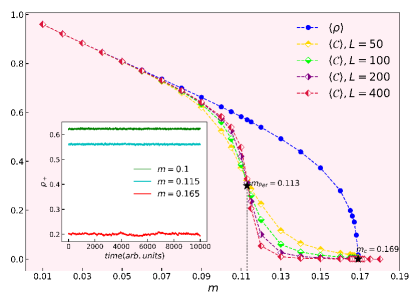
Figure 1: Evolution of vegetation dynamics. Inset: The typical evolution of the living cell density $\rho(t)$ for several values of the mortality rate $m$. From top to bottom, the mortality rates are set as $m=0.100$, $m=0.115$, and $m=0.165$. The linear lattice size is $L=100$, and the time unit corresponds to one iteration step. Main figure: The average of the vegetation density $\langle\rho\rangle$ for $L=100$ and the relative size of the largest cluster $\langle\mathcal{C}_{max}\rangle$ for $L=50,100,200,400$ versus the mortality rate $m$. The black star symbol represents the percolation threshold $m_{Per}=0.113$, which is determined from the crossing point for the various system sizes.

II.2 Modeling the seasonal effects

So far, we have considered a SCA model with a constant mortality rate. However, for actual, realistic vegetation dynamics, one has to include the effect of seasonal cycles. To address this, we introduce a time-dependent, periodic mortality rate $m(t)$. In order to model the time dependency, we use a simple sinusoidal form for the mortality parameter:

$$m(t)=m_{0}+Asin(2\pi t/T+\phi)\hskip 14.22636ptt>t^{*}$$ (5)

Specifically, we are interested in investigating whether an ecosystem that seasonally is put in a situation of high environmental stress is able to recover, as well as the conditions that need to be satisfied to avoid a permanent transition to a desertified state.

In our analysis, starting from a randomly generated configuration, we first let the system equilibrate with a constant mortality parameter $m_{0}$. At time $t^{*}$, we apply the time-dependent $m(t)$, which consists of a constant component, $m_{0}$, as well as an oscillatory term with amplitude $A$, period $T$, and phase $\phi$. Here we consider $m_{0}=0.16$, $\phi=0$, $T=5000$, with $T$ chosen to be sufficiently large to be greater than the time scale of the internal fluctuations of $\rho$. It is worth noting that the initial value $m_{0}$ has been intentionally set just below the desertification transition point $m_{c}=0.169$. This is specifically chosen in order to determine the effects of periodic increases in environmental stress and whether they can drive a transition to a non-recoverable dead or barren state. To this end, we investigate the impact of increasing the amplitude $A$ on the behavior of $\rho$, signifying, for example, an increase in climate fluctuations and seasonal extreme weather events.

The inset of Fig. 2 shows the effects of different amplitude values ($A=0.005,0.01,0.015$) on the vegetation density. Interestingly, we show that even when the time-dependent mortality rate goes above the critical value, the system can recover its alive vegetation cover and continue to respond to the oscillating $m(t)$, as long as the amplitude of the oscillation, and thus the time spent in a condition where $m(t)>m_{0}$, is sufficiently small. We find a crossover amplitude $A_{c}$ such that for $A>A_{c}$ the system enters a state of almost all dead or degraded cells and is no longer able to recover, even though the environmental stress $m(t)$ strongly decreases afterwards. The drop to a dead or degraded configuration is related to the system’s fluctuations near the crossover point, with increasingly long metastable oscillating states. We additionally note that the response delay is very small in the system sizes considered.

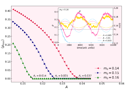
Figure 2: Evolution of vegetation dynamics for time-dependent mortality rate $m(t)$. Inset: Vegetation density $\rho$ (left y-axis) and time-dependent mortality rate $m(t)$ (dashed lines, right y-axis) as a function of the time. The parameters used are as follows: an initial mortality rate of $m_{0}=0.16$, the lattice size $L=100$, a period of $T=5000$, and three different amplitudes, namely $A=0.005,0.01$, and $0.015$. Main figure: Evolution of the mean value of the minima of the vegetation density $\langle\rho_{min}\rangle$ as a function of the amplitude $A$ for $T=5000$ with $m_{0}=0.14,0.15$, and $m_{0}=0.16$. We show the respective amplitudes $A_{c}(m_{0},T)$ highlighting the points where the curves drop to $0$.

The numerical computation is performed for a fixed period of $T=5000$, varying $m_{0}$ and $A$, and $10^{6}$ time steps. For each value, we determine the values of $\rho_{min}$, minimum vegetation density for each period. This corresponds to the minimum vegetation fraction, which happens at the time of highest seasonal stress for each period. We use a cubic spline interpolation to determine the minima for each period. Figure 2 shows $\langle\rho_{min}\rangle$, the average minimum across all periods, as a function of the amplitude $A$ for $m_{0}=0.14,0.15$, and $0.16$. A crossover to desertification is observed as $\langle\rho_{min}\rangle$ reaches zero. In Fig. 2, we observe the crossover amplitude points $A_{c}(m_{0},T)$ at which desertification takes place, which for $m_{0}=0.14,0.15$, and $0.16$, are respectively $0.0375,0.0255$, and $0.0145$.

We also find that the system’s behavior and crossover to desertification is influenced by the period $T$, with shorter oscillations (compared to the system’s own intrinsic time scales) resulting in a more robust alive phase. The results can be found in Text II and Fig. S2 of the supplementary material.

III Finding vegetation clusters through satellite data

The wealth of data from earth observation satellites offers the chance to recognize the patterns of vegetation cover in real ecosystems. In this section, we apply the clustering analysis used in the previous section on the cellular automaton model on real satellite imagery with the aim of recognizing areas of vulnerability due to fragmented vegetation.

We use two vegetation indices commonly used to detect vegetation from satellite imagery: the Normalized Difference Vegetation Index (NDVI) Pettorelli (2013) and the Leaf Area Index (LAI) Fang et al. (2019). NDVI is widely used in ecosystem monitoring due to its simple formulation. It measures the vegetation greenness by calculating the ratio of spectral reflectances in near-infrared and red light. Green, living plants have a high reflection in the near infrared and high absorption in red and visible light frequencies, which is a markedly different response than bare soil, water, snow, or urbanized areas. For this reason, it is commonly used in remote sensing to qualitatively assess vegetation health and density in a specific area. We also use the LAI data, which quantifies the thickness of vegetation cover and is defined as half the total area of green elements in the canopy per unit of ground area. This quantity is obtained either through direct measurement (performed locally on a sampling basis) or through indirect methods such as image analysis. The data for this project is extracted from the European database Copernicus Global Land Service, which provides comprehensive global vegetation products JRC (2023).

The NDVI and LAI images were acquired from the Copernicus Land dataset three times per month: for NDVI on the $1^{st}$, $11^{th}$, and $21^{st}$ day of each month spanning the time period from $2014$ to $2020$, while for LAI on the $10^{th}$, $20^{th}$, and last day of each month, from $2014$ up until August $2020$ (there are gaps in the LAI data during the winter and autumn seasons, due to insufficient illumination in satellite observations). Our analysis focuses on specific regions, namely in France, Germany, Ireland, Spain, and Greece. We note that drylands are particularly present in Spain and Greece. We pre-processed the images in the dataset in order to normalize the individual image pixel data, a greyscale image with values from 0 to 255, to $[0,1]$ for land areas. Additionally, we exclude sea and lake areas: large water areas are marked in both datasets (having been assigned the maximum pixel value 255), while lakes need to be manually excluded using a Threshold-Sauvola approach Sauvola and Pietikäinen (1997), which is a local thresholding method (see the supplementary material for more detail).

Finally, we note that the data used is composed of a mosaic corrected for atmospheric differences, including the removal of cloud coverage. Here, for the purpose of simplification, we do not consider the possible systematic effect of human activities (e.g. farming, grazing, constructions) on the analysis of vegetation clusterization.

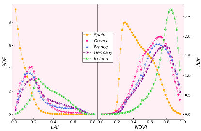
Figure 3: Probability distribution of normalized NDVI and LAI pixel values across examined land regions. The data is aggregated over several samples taken at different dates and times. Notably, Spain exhibits a distinct distribution pattern in both datasets, characterized by a lower vegetation or leaf cover compared to the neighboring countries.

III.1 Spatial distribution of vegetation and breakdown into clusters

In order to determine the quality of the vegetation cover, and whether the overall environmental stress is high enough to drive a geographical area into a degradation and desertification process, we analyze the satellite images of vegetation in order to identify a breakdown into disconnected clusters. Specifically, here we look for a breakdown in connectivity, which in the vegetation model used in Section II translates to a percolation transition, as an early warning signal of the desertification process.

As a starting point, we show in Fig. 3 the Probability Distribution Function (PDF) of NDVI and LAI pixels intensity across the analyzed regions. It is just worth noting that LAI is a curated index, deriving from a mix of indirect and direct measurements, and it is not directly and quantitatively comparable to NDVI. It is however evident that both indices signal the presence of vegetation in a large fraction of the samples (which, here, include the whole countries), with especially intense vegetation in Ireland (green line, NDVI only due to data availability), and less vegetation intensity in Spain due to the climate and morphological characteristics of the country.

A crucial simplification that we need to introduce as we process NDVI or LAI images, which for a single pixel corresponds to an intensity between 0 and 1, is the discretization of the data. To this aim, we introduce a cut-off parameter $\lambda$, which classifies the pixels as either "vegetated"/"living" (for values $>\lambda$) or "non-vegetated"/"dead" (for values $<\lambda$). Note that we do not distinguish between the dead and degraded state as in Section II as we cannot determine this qualitative difference in the bare soil from the satellite data alone. A good choice of the cut-off value $\lambda$ is important in effectively distinguishing vegetation from non-vegetation. Therefore, as our first step we identify a cut-off $\lambda$ for each region; note that different regions may have different $\lambda$ values due to differences in vegetation type and thus NDVI or LAI intensity. A suitable range for $\lambda$ can simply be established from Fig. 3, by making sure that the typical value of NDVI or LAI (i.e. the peak of the distribution) lies to the right of the cut-off $\lambda$. Both the vegetation density $\rho$ and the size of vegetated clusters will depend on the chosen $\lambda$ (see Fig. 4). The average vegetation density, averaged over several time samples, approximately linearly decreases as a higher cut-off is considered. However, the average size of the largest cluster $\mathcal{C}$, exhibits a plateau at values $\lambda\approx 0.7$ to $0.8$. The clusterization analysis will thus not depend too strongly on the exact value of $\lambda$, and we choose a value of $\lambda$ around the start of said plateau.

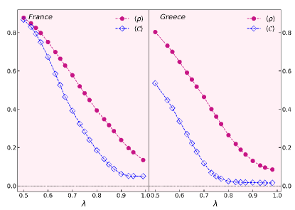
Figure 4: Average vegetation density $\langle\rho\rangle$ and average relative size of the largest cluster $\langle\mathcal{C}\rangle$ as a function of the cut-off $\lambda$ used to discriminate between alive and dead sites in NDVI satellite data. We show two example regions: France (left) and Greece (right). The average is performed over several samples taken at different dates and times.

III.2 Analysis of NDVI time series

The key quantities that we analyze are the fraction of alive vegetation, or vegetation density $\rho$, and the size of the largest vegetation cluster, rescaled with the total size of the sample image, $\mathcal{C}$. We note that the values of $\mathcal{C}$ and $\rho$ have been normalized to the land area, excluding water bodies.

Here we focus on NDVI data specifically for areas in Greece and France, as representatives for lands more and less subject to soil degradation and the presence of semiarid conditions; we refer to the Supplementary material for more areas and additional LAI data. We consider the vegetation density $\rho$ and the relative size of the largest cluster $\mathcal{C}$ over time. NDVI data for France and Greece is analyzed in Fig. 5. In the plot related to France (top panel), there is an overlap between $\rho$ and $\mathcal{C}$, indicating that nearly all the vegetated pixels belong to the largest cluster of vegetation, hence meaning low mortality rate, low environmental stress, and healthy soil conditions. Additionally, we note a seasonal periodic behavior in both $\rho(t)$ and $\mathcal{C}(t)$. 2015 and 2016 autumns and winters show particularly fragmented vegetation, where the largest cluster consistently comprised up to one order of magnitude less than the vegetated fraction. Thus, in the context of general health, we can identify those situations as ones of temporary stress.

In contrast, when examining areas in Greece (bottom panel in Fig. 5), a gap between $\rho$ and $\mathcal{C}$ becomes systematically apparent, evidencing a fragmented vegetation pattern. Crucially, $\mathcal{C}$ not scaling as $\rho$ signals the absence of a percolating phase and thus heralds potential soil health issues in this region under climate stress. The same analysis can be performed on LAI image data (see Supplementary material); LAI is less sensitive to noise and exhibits a smoother periodic behavior over seasons. The qualitative difference between the France and Greece samples is also evident from the largest cluster analysis of LAI images.

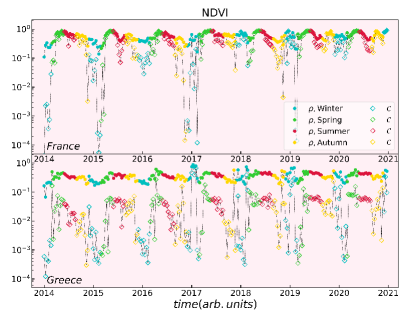
Figure 5: Comparison of vegetation density $\rho$ and the relative size of the largest cluster $\mathcal{C}$ of NDVI data as a function of time, between 2014 and 2021. Top panel: France; bottom panel: Greece. For both samples, we use a cutoff value of $\lambda=0.7$.

IV Detecting vegetation stress

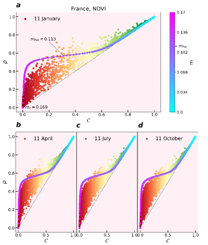
Figure 6: Vegetation density $\rho$ and the relative size of the largest cluster $\mathcal{C}$ for $30km\times 30km$ areas in France. The four panels (a)-(d) present the data for the $11^{th}$ of January, April, July, and October respectively, covering the period from 2014 to 2020. We use a cutoff value $\lambda=0.8$. The diagonal $\rho=\mathcal{C}$ is shown, as well as the curve of the $(m,\rho,\mathcal{C})$ data points obtained from the numerical simulation of the SCA model (the values of $m$ are represented through a color scale). The points are color coded by their distance from $\mathcal{C}=0$. The desertification threshold $m_{c}=0.169$ is highlighted in the plot.

In this section, we show how we can integrate the satellite image analysis with the signs of degradation obtained by the analysis of clusterization in the SCA model in eqs. (1)-(4). On one hand, we have shown how the degradation transitions can be driven by a single parameter, the mortality rate of the vegetation. In real-world data, the environmental stress is affected by season, and any additional causes may be considered as fluctuations on top of them. We aim here to identify the areas that show vulnerability: these areas will have a relatively dense vegetation, but broken down into many small clusters. As shown in section II, this is a percolation transition that precedes the situation where vegetation is not surviving.

Here we consider sub-images of size $100\times 100$ pixels, that is $30km\times 30km$ areas. We take an image per season ($4$ images per year) for years $2014$ to $2020$. For each sample, we obtain the vegetated fraction $\rho$ and the size of the largest cluster $\mathcal{C}$. There are three main scenarios: Firstly, when we encounter areas with high $\rho$ and $\mathcal{C}$, it is an indication of regions with low mortality rate: this corresponds to a large portion of the image covered by unbroken, percolating vegetation. The second case corresponds to regions characterized by low $\rho$ and $\mathcal{C}$ values. These areas thus have low vegetation coverage, which include genuinely degraded land, rocky terrains, and urban areas. The last case involves instances of high $\rho$ values but low $\mathcal{C}$ values. This combination suggests that despite the presence of relatively dense vegetation, the environmental stress and thus the mortality rate is high, causing the vegetation to break down into small clusters, as a precursor to full degradation. We show in Fig. 6 a scatter plot of $\rho$ against $\mathcal{C}$ for all image samples obtained for France. We aggregate all results for each season.

The real-world data points obtained from satellite images can be compared with two guidelines. The first is the line $\rho=\mathcal{C}$, which corresponds to a fully connected vegetation. This represents a low mortality rate situation and the maximum value $\mathcal{C}$ can be. Thus, all data points will lie in the $\rho>\mathcal{C}$ sector. Moreover, using eqs. (1)-(4), we can obtain the curve $(m,\langle\rho\rangle,\langle\mathcal{C}\rangle)$ by considering several realizations of the SCA model and extracting the centroid of data for a given $m$ value.

Figure 7: Qualitative assessment of land degradation, obtained by comparing each sample’s vegetation density and largest vegetation cluster size to the cellular automata vegetation growth model (1)-(4). The color coding refers to the value of $\mathcal{C}$ for each sample and is shown here for France on 11 June 2020 for $\lambda=0.75$.

The data points in Fig. 6 approximately lie between the top of the numerical curve obtained from the numerical simulations of the SCA model and the diagonal $\mathcal{C}=\rho$. In order to understand the significance in terms of environmental stress, we should first highlight the systematic effect of permanently unvegetated pixels in each sample. These pixels might correspond to locations not covered by soil, e.g. urban or rocky areas. These reduce the effective available size of each sample, in a way that is not accounted by the model (as these pixels are not recoverable even in the most favorable conditions). This explains the presence of data points close to the diagonal for even mid and low values of $\mathcal{C}$. As well, points spread between the diagonal and the numerical curve correspond to increasingly degraded samples with reduced effective size. One could attempt to quantify this systematic effect by introducing stochastically arranged blocked pixels in the numerical model; we leave this detailed analysis to future work. Here, we give a simple qualitative assessment of the degradation scenario by evaluating the distance from the diagonal. Given the position of the points with respect to the diagonal and the numerical curve as outlined above, we classify the data points in three levels of vegetation health. The healthiest vegetation corresponds to the top right area, where the vegetation is above the percolation transition. The points in the bottom left area have few vegetated pixels, broken down into small non-percolating clusters, which therefore have the lowest vegetation health. The points in the lower central area, close to the diagonal but with smaller vegetation density, have intermediate vegetation health due to the reduced effective soil availability. We show this qualitative classification by color coding each sample with its $\mathcal{C}$ value in Fig. 7 for areas in France, superimposed to a map of the land that has been analyzed.

V Conclusions and future outlooks

We have highlighted the agreement between vegetation clusters detected through satellite image analysis and a SCA model of vegetation growth, effectively capturing the dynamics of patchiness as they are associated with environmental stress and potential land degradation susceptibility. By analyzing vegetation density and cluster size, we recognized two significant transitions: percolation and degradation. We found instances of the intermediate phase, where the vegetation is fragmented, in real ecosystems. Moreover, we numerically investigated the impact of seasons on vegetation dynamics through a time-dependent mortality parameter. Our simulations demonstrated that oscillations in the mortality rate act as a protective measure against desertification, allowing for recovery.

An important next step is considering the influence of areas where vegetation is not permitted to grow, both due to natural and artificial conditions (e.g. cities and rocky lands). Preliminary analysis suggests that the presence of blocked pixels in a cellular automata model for vegetation growth affects the breakdown in clusters and the percolation transition point. A future analysis will be focused on quantitatively interpreting this effect as it is associated with the real-world data obtained from satellite images, allowing to quantitatively understand land degradation dynamics in several geographical areas.

Supplementary Material

I An in-depth look at the degradation transition in the SCA model

In the SCA model, when implementing equations (1)-(4) outlined in the main text, there are various approaches to consider for the transition of dead cells $(0)$. It is important to note that the sum of transition probabilities must satisfy the condition $W_{00}+W_{0+}+W_{0-}=1$.

In the following, to identify the nature of the desertification transition at the critical mortality rate $m_{c}$, we conduct an analysis of the mean vegetation density $\langle\rho\rangle$ and the root-mean-square deviation of $\rho$ fluctuations $\sigma_{\rho}$ as functions of the mortality rate $m$. The insets in Fig. S1a,b depict $\langle\rho\rangle$ and $\sigma_{\rho}$ plotted against $m$ on linear scales, respectively. It is evident that as $m$ increases, $\langle\rho\rangle$ approaches zero, indicating a continuous transition. Conversely, $\sigma_{\rho}$ shows a significant rise near $m_{c}$, suggesting a potential transition. In Figure S1a, the average value $\langle\rho\rangle$ is plotted on a logarithmic scale against the absolute difference $|m-m_{c}|$. The numerical data exhibit a remarkable fit when described by a power law with a slope of $0.42\pm 0.01$. The logarithmic plot of $\sigma_{\rho}$ as a function of $|1-m_{c}/m|$ is presented in Figure S1b. In this case, the numerical data also conform well to a power law with a slope of $-0.29\pm 0.01$.

II Influence of period $T$ in time-dependent mortality rate $m(t)$ on System Behavior

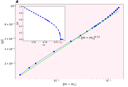
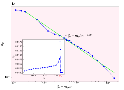
Figure S1: (a) Inset: The average density of living cells $\langle\rho\rangle$ as a function of $m$ on a linear scale. Main: A log-log plot of $\langle\rho\rangle$ vs $|m-m_{c}|$. The green solid line represents the best-fit line, corresponding to a power law with a slope of $0.42\pm 0.01$. (b) Inset: The root-mean-square deviation of the living cell density $\sigma_{\rho}$ as a function of mortality rate $m$ on a linear scale. Main: A logarithmic plot of $\sigma_{\rho}$ vs $|1-m_{c}/m|$. The green solid line represents the best-fit line, corresponding to a scaling law with a slope of $-0.29\pm 0.01$

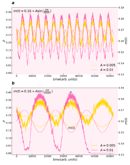
Figure S2: Vegetation density $\rho$ (left y-axis) and time-dependent mortality rate $m(t)$ (right y-axis) as functions of time. The parameters used are as follows: initial mortality rate $m_{0}=0.16$, lattice size $L=100$, and two different amplitudes: $A=0.005$ and $A=0.01$. (a) Short period $T=5000.$ (b) Larger period $T=20000$.

In the main text, we focus our analysis on a specific period, $T=5000$. In Figure S2, the plots of $\rho$ (right y-axis) and $m(t)=m_{0}+Asin(2\pi t/T+\phi)$ (left y-axis) as functions of time are presented. Here, we consider $m_{0}=0.16$ and examine two different values for the amplitude $A$: $A=0.005$ and $A=0.01$. In Fig. S2a, we set $T=5000$, while in Fig. S2b, we use the period $T=20,000$. Fig. S2 clearly demonstrates that the system’s behavior and the critical point of the degradation transition are influenced by the chosen period $T$. For $A=0.01$, the system remains stable with $T=5000$ (Fig. S2a), but drops to zero with $T=20,000$ (Fig. S2b). This observation can be explained by the system’s tendency to converge towards zero when the mortality parameter $m$ exceeds a critical value $m_{c}$. A small value of $T$ amplifies the oscillation term and prevents the system from entering the desertified regime when $m>m_{c}$. Conversely, a large $T$ leads to failure in recovery. Hence, besides identifying the critical value of $m$ in the static regime, there appears to be a critical value for $T$ in the time-dependent regime.

III Removing lakes from satellite images using adaptive thresholding: A Threshold-Sauvola approach

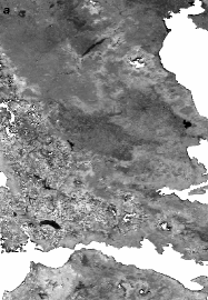
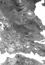
Figure S3: NDVI-based representation of Greece’s vegetation patterns at a specific time. Left panel: The original image. Right panel: The outcome of applying the threshold-Sauvola method.

We aim to analyze vegetation dynamics using two indices: the Normalized Difference Vegetation Index (NDVI) Pettorelli (2013) and the Leaf Area Index (LAI) Fang et al. (2019). To acquire the necessary data, we access the Copernicus Global Land Service JRC (2023) website, which is the European Union’s Copernicus Earth observation program database for comprehensive global vegetation products. Within this dataset, the pixel values for the NDVI analysis range from $0$ to $254$. We normalize the pixel values by dividing them by the maximum value observed in the dataset. Importantly, the highest pixel value within our dataset represents regions occupied by seas and oceans (as marked by the database pre-processing), and pixels falling below a certain threshold denote lakes and other bodies of water that have not been automatically removed by the database pre-process. Higher positive values indicate the existence of dense vegetation. In order to concentrate only on vegetation, we need to exclude water bodies from our analysis. The most successful method for identifying the threshold to remove the lakes from our dataset is the Threshold-Sauvola method Sauvola and Pietikäinen (1997), a specialized and local thresholding algorithm. This technique takes into account local variations in image intensity and adaptively adjusts the threshold value accordingly Sauvola and Pietikäinen (1997). The processed images depicting NDVI data in Greece on a specific day can be observed in Fig. S3a before applying the method, while Fig. S3b displays the image after the application.

IV Analysis of NDVI and LAI data in all the studied regions

We include here the geographical coordinates, as well as the dimensions of the satellite images specific to each region under study in Table 1.

Table 1: Geographical coordinates and dimensions of the satellite images for each region

Region	Latitude Range	Longitude Range	Image Dimensions
France	$43.6009$ to $49.2776$	$-0.6392$ to $5.8648$	$1907$ $\times$ $2185$
Germany	$50.7715$ to $53.4145$	$7.3127$ to $13.8169$	$888$ $\times$ $2185$
Ireland	$52.2316$ to $54.0387$	$-9.0896$ to -$6.4198$	$607$ $\times$ $897$
Spain	$37.7445$ to $42.3097$	$-6.2500$ to $-0.8152$	$1534$ $\times$ $1826$
Greece	$37.8524$ to $40.6447$	$21.0865$ to $23.0171$	$938$ $\times$ $649$

In the main text, we primarily show results with NDVI data. Now, we shift our attention toward examining the LAI data. LAI Fang et al. (2019) measures half of the total green surface area within the canopy per unit of horizontal ground area. This index encompasses all layers of the canopy, including the understory, which plays a crucial role in forested regions. Essentially, the LAI provides a quantitative measure of vegetation cover thickness and extent. The LAI images obtained from the aforementioned database exhibit pixel values ranging from $0$ to $255$. To ensure consistency with our methodology, we apply the Threshold-Sauvola technique to exclude lakes from the analysis and subsequently conduct a similar investigation as done with NDVI on the LAI images.

We follow the procedure outlined in Section III of the main text to determine reasonable values of the cutoff $\lambda$ to discretize the image intensity data. We note that LAI generally has lower values with respect to NDVI. We thus determine the following good ranges for the values of the cut-off parameter. For NDVI: France, $0.75$ to $0.85$; Germany, $0.8$ to $0.9$; Spain, $0.5$ to $0.6$; Greece, $0.7$ to $0.8$; and Ireland, values from $0.85$ to very close to $1$. For LAI: France, $0.2$ to $0.3$; Germany, $0.25$ to $0.35$; Spain, $0.1$ to $0.2$; Greece, $0.2$ to $0.3$; and Ireland, $0.25$ to $0.35$;

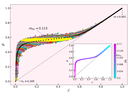
Figure S4: $\rho$ vs $\mathcal{C}$ for simulated samples of the cellular automata model, for increasing values of the mortality rate $m$ on a lattice of size $L=100$. Inset: Centroids of each cloud of points for a given value of $m$. The mortality rate $m$ is color coded on the $\rho$ vs $\mathcal{C}$ curve.

In Fig. 6 of the main text we show the curve relating the vegetation density $\rho$ and the relative size of the largest cluster $\mathcal{C}$ with the mortality rates $m$ for the SCA model (1)-(4). This theoretical model curve is plotted based on cloud centroids obtained from Fig. S4, which shows $\rho$ as a function of $\mathcal{C}$. This graph depicts a collection of clouds, each corresponding to a value of $m$ represented by its own color. Within each cloud, there are $10000$ data points representing distinct memoryless time steps in the numerical simulation. Near the degradation threshold $m_{c}$ we run the simulation for $300,000$ time steps. This was done to guarantee that the value of $\rho$ reaches zero, thereby capturing the critical dynamics of desertification. As shown in Fig. S4, for low values of $m$ there is minimal dispersion observed around the clouds. However, as the value of $m$ increases, the fluctuations of $\mathcal{C}$ become more pronounced, reaching maximum dispersion at the percolation transition point $m_{Per}=0.113$ (depicted as the large yellow cloud in Fig. S4). For higher values of $m$, the fluctuations gradually decrease until reaching $m_{c}$ at coordinates $(0,0)$, suggesting the complete absence of vegetation in the system. For better clarity in the plot, a dotted line $x=y$ has been included that serves as a reference, noting that data points cannot exist below this line. In Fig. S4, black crosses represent the centers of the clouds. Additionally, in the inset of Fig. S4, the centroids are presented once again, with a color scale showing the corresponding value of the mortality rate $m$.

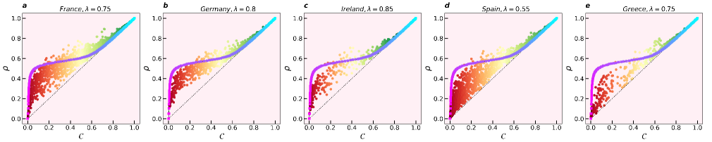
Figure S5: Vegetation density $\rho$ and relative size of the largest cluster $\mathcal{C}$ for NDVI data on 11 June 2014-2020 for some regions. The points are color coded by their distance from $\mathcal{C}=0$.

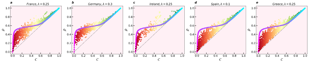
Figure S6: Vegetation density $\rho$ and relative size of the largest cluster $\mathcal{C}$ for LAI data on 10 June 2014-2020 for some regions. Due to the limited size of the complete Ireland dataset, we have extended the plotted period beyond a single day.

Figures S5 and  S6 provide the scatter plots of the vegetation density $\rho$ and the relative size of the largest cluster $\mathcal{C}$ for various regions, for both NDVI and LAI data, respectively. These figures also include a comparison with the SCA model. The data is collected on the $11^{th}$ and $10^{th}$ day of June spanning from $2014$ to $2020$ for NDVI and LAI, respectively. Each data point on the graph represents a sub-image measuring $100\times 100$ pixels. The same considerations used in the main text for Fig. 6 (NDVI data for France) are applicable here to qualitatively connect each data point with its corresponding scenario of environmental stress. Finally, in Figures S7 and S8 we show the sub-images superimposed to a map of the analyzed area, color coded with the value of $\mathcal{C}$ for each sample. This qualitatively estimates the vegetation stress for all the analyzed areas in several European countries, for both NDVI and LAI data.

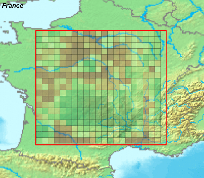
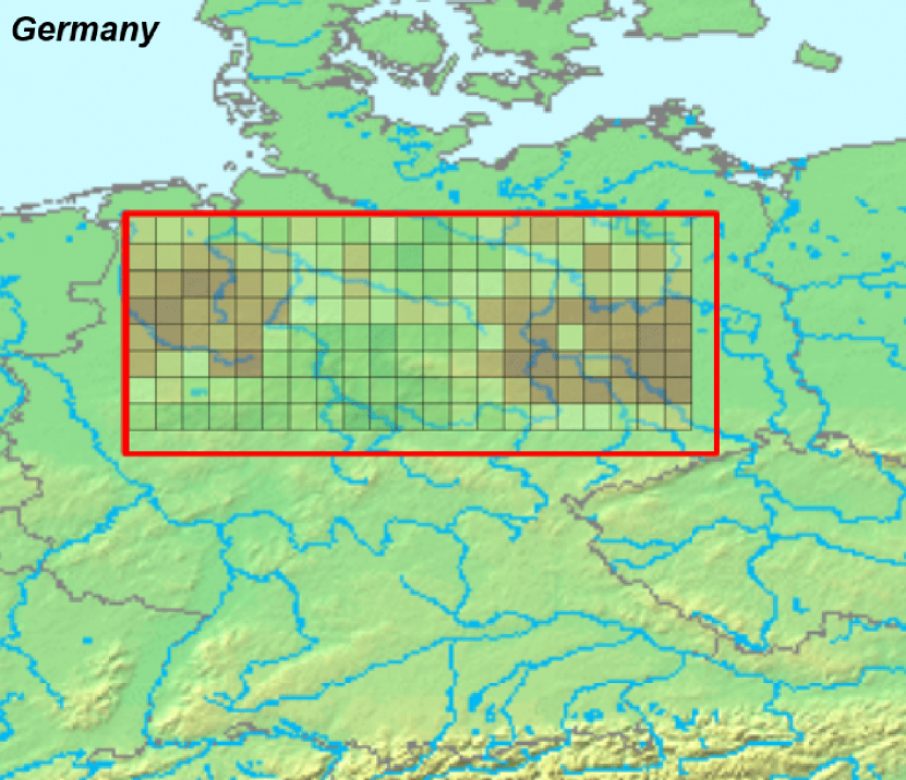
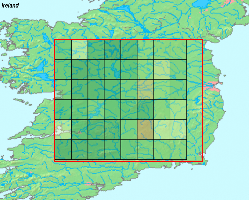
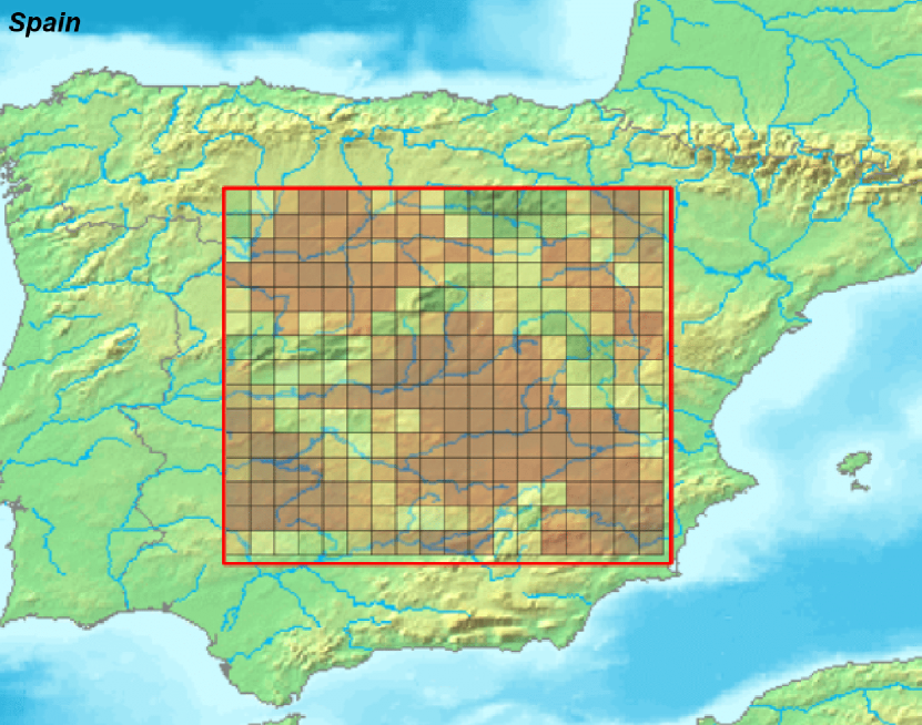
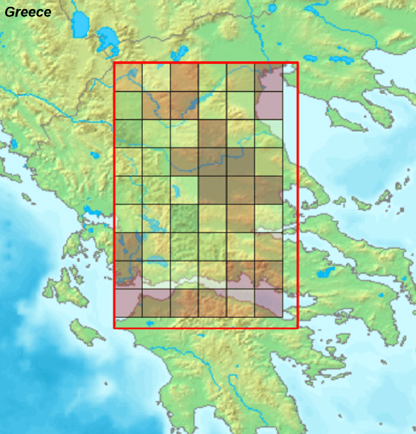
Figure S7: Qualitative assessment of land degradation, using the value of $\mathcal{C}$ for each sample. The data shown here is obtained from the NDVI on 11 June 2020. From top left to bottom right: France ($\lambda=0.75$), Germany ($\lambda=0.8$), Ireland ($\lambda=0.85$), Spain ($\lambda=0.55$), Greece ($\lambda=0.75$).

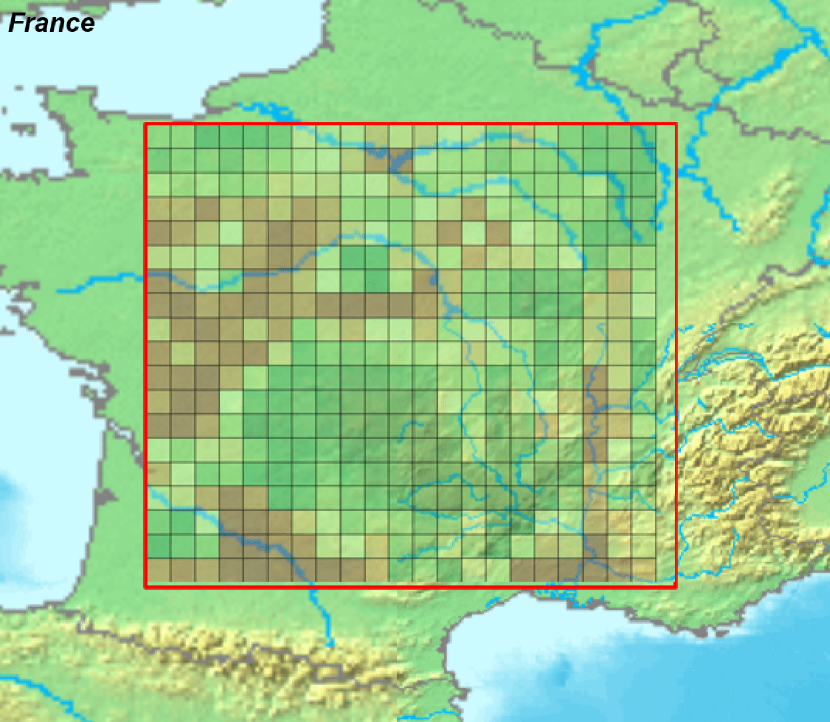
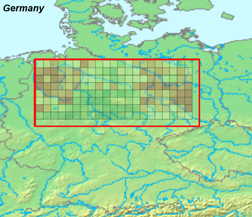
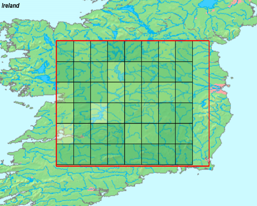
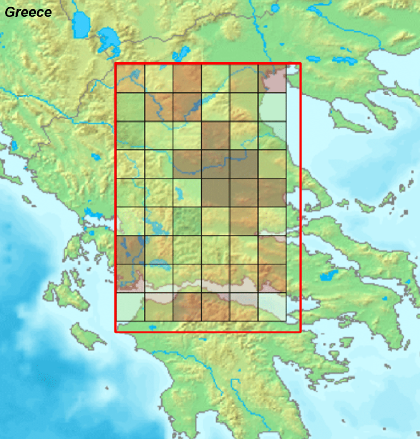
Figure S8: Qualitative assessment of land degradation, using the value of $\mathcal{C}$ for each sample. The data shown here is obtained from the LAI on 10 June 2020. From top left to bottom right: France ($\lambda=0.25$), Germany ($\lambda=0.3$), Ireland ($\lambda=0.25$), Spain ($\lambda=0.1$), Greece ($\lambda=0.25$).

References

- von Hardenberg et al. (2001) J. von Hardenberg, E. Meron, M. Shachak, and Y. Zarmi, Physical Review Letters 87, 198101 (2001).
- Shnerb et al. (2003) N. Shnerb, P. Sarah, H. Lavee, and S. Solomon, Physical Review Letters 90, 038101 (2003).
- Kéfi et al. (2007a) S. Kéfi, M. Rietkerk, M. Van Baalen, and M. Loreau, Theoretical population biology 71, 367 (2007a).
- Kéfi et al. (2007b) S. Kéfi, M. Rietkerk, C. L. Alados, Y. Pueyo, V. P. Papanastasis, A. ElAich, and P. C. De Ruiter, Nature 449, 213 (2007b).
- Note (1) The categorization of land regions into arid, semi-arid, and dry sub-humid climatic zones is based on aridity indices (e.g., Thornthwaite and Palmer Drought Severity Index) and Holdridge life zones, considering factors such as precipitation and potential evapotranspiration Dregne and Chou (1992); McMahon et al. (2013).
- Hobbs and Huenneke (1992) R. J. Hobbs and L. F. Huenneke, Conservation Biology 6, 324 (1992).
- Levick and Asner (2013) S. R. Levick and G. P. Asner, 157, 121 (2013).
- Dahlin et al. (2013) K. M. Dahlin, G. P. Asner, and C. B. Field, 110, 6895 (2013).
- Asner et al. (2013) G. P. Asner, J. R. Kellner, T. Kennedy-Bowdoin, D. E. Knapp, C. Anderson, and R. E. Martin, PloS one 8, e60875 (2013).
- Reynolds et al. (2007) J. F. Reynolds, D. M. S. Smith, E. F. Lambin, B. Turner, M. Mortimore, S. P. Batterbury, T. E. Downing, H. Dowlatabadi, R. J. Fernández, J. E. Herrick, et al., science 316, 847 (2007).
- Sala et al. (2000) O. E. Sala, F. Stuart Chapin, J. J. Armesto, E. Berlow, J. Bloomfield, R. Dirzo, E. Huber-Sanwald, L. F. Huenneke, R. B. Jackson, A. Kinzig, et al., science 287, 1770 (2000).
- Archer et al. (2001) S. Archer, T. W. Boutton, and K. A. Hibbard, in Global biogeochemical cycles in the climate system (Elsevier, 2001) pp. 115–137.
- Jensen (2009) J. R. Jensen, Remote sensing of the environment: An earth resource perspective (Pearson Education, 2009).
- Goodchild (1991) M. F. Goodchild, Progress in Human geography 15, 194 (1991).
- Tague and Band (2004) C. L. Tague and L. E. Band, Earth interactions 8, 1 (2004).
- Grimm et al. (2006) V. Grimm, U. Berger, F. Bastiansen, S. Eliassen, V. Ginot, J. Giske, J. Goss-Custard, T. Grand, S. K. Heinz, G. Huse, et al., Ecological modelling 198, 115 (2006).
- Elith* et al. (2006) J. Elith*, C. H. Graham*, R. P. Anderson, M. Dudík, S. Ferrier, A. Guisan, R. J. Hijmans, F. Huettmann, J. R. Leathwick, A. Lehmann, et al., Ecography 29, 129 (2006).
- Kéfi et al. (2010) S. Kéfi, M. B. Eppinga, P. C. de Ruiter, and M. Rietkerk, Theoretical Ecology 3, 257 (2010).
- Kéfi et al. (2014) S. Kéfi, V. Guttal, W. A. Brock, S. R. Carpenter, A. M. Ellison, V. N. Livina, D. A. Seekell, M. Scheffer, E. H. Van Nes, and V. Dakos, PloS one 9, e92097 (2014).
- Rietkerk and Van de Koppel (2008) M. Rietkerk and J. Van de Koppel, Trends in ecology & evolution 23, 169 (2008).
- Martinez-Garcia et al. (2023) R. Martinez-Garcia, C. Cabal, J. M. Calabrese, E. Hernández-García, C. E. Tarnita, C. López, and J. A. Bonachela, Chaos, Solitons & Fractals 166, 112881 (2023).
- Corrado et al. (2014) R. Corrado, A. M. Cherubini, and C. Pennetta, Physical Review E 90, 062705 (2014).
- Manor and Shnerb (2008) A. Manor and N. M. Shnerb, Journal of theoretical biology 253, 838 (2008).
- Von Hardenberg et al. (2010) J. Von Hardenberg, A. Y. Kletter, H. Yizhaq, J. Nathan, and E. Meron, Proceedings of the Royal Society B: Biological Sciences 277, 1771 (2010).
- Rietkerk and van de Koppel (1997) M. Rietkerk and J. van de Koppel, Oikos , 69 (1997).
- Meloni et al. (2019) F. Meloni, G. M. Nakamura, C. R. Granzotti, and A. S. Martinez, Physica A: Statistical Mechanics and its Applications 534, 122048 (2019).
- Pettorelli (2013) N. Pettorelli, The normalized difference vegetation index (Oxford University Press, 2013).
- Fang et al. (2019) H. Fang, F. Baret, S. Plummer, and G. Schaepman-Strub, Reviews of Geophysics 57, 739 (2019).
- JRC (2023) E. C. JRC, (2023).
- Sauvola and Pietikäinen (1997) J. Sauvola and M. Pietikäinen, Pattern Recognition 33, 225 (1997).
- Dregne and Chou (1992) H. E. Dregne and N.-T. Chou, Degradation and restoration of arid lands 1, 73 (1992).
- McMahon et al. (2013) T. A. McMahon, M. C. Peel, L. Lowe, R. Srikanthan, T. R. McVicar, L. Barring, and F. H. Chiew, Hydrology and Earth System Sciences 17, 1331 (2013).