SR-PredictAO: Session-based Recommendation with High-Capability Predictor Add-On

Abstract

Session-based recommendation, aiming at making the prediction of the user’s next item click based on the information in a single session only even in the presence of some random user’s behavior, is a complex problem. This complex problem requires a high-capability model of predicting the user’s next action. Most (if not all) existing models follow the encoder-predictor paradigm where all studies focus on how to optimize the encoder module extensively in the paradigm but they ignore how to optimize the predictor module. In this paper, we discover the existing critical issue of the low-capability predictor module among existing models. Motivated by this, we propose a novel framework called Session-based Recommendation with Predictor Add-On (SR-PredictAO). In this framework, we propose a high-capability predictor module which could alleviate the effect of random user’s behavior for prediction. It is worth mentioning that this framework could be applied to any existing models, which could give opportunities for further optimizing the framework. Extensive experiments on two real benchmark datasets for three state-of-the-art models show that SR-PredictAO out-performs the current state-of-the-art model by up to 2.9% in HR@20 and 2.3% in MRR@20. More importantly, the improvement is consistent across almost all the existing models on all datasets, which could be regarded as a significant contribution in the field.

I Introduction

Next-item recommender systems show their importance in the current age of e-commerce by accurately predicting the user’s subsequent behavior. Session-based recommendation is one recent hot topic of the next-item recommender. It is different from the general next-item recommendation systems, which put great attention on a specific group of existing users with a large number of historical behavior records to perform the next-item prediction. The session-based recommendation, as its name indicates, groups all the activities in the basic unit of the session and is based only on the information within a single session. The idea of session-based recommendation systems comes from [1]. It shows that intra-session-dependencies have a more significant impact than inter-session dependencies on the user’s final decision to view the next item. In particular, the user’s next-item behavior is usually related to behaviors in the current session. For example, a user’s behavior in buying phone accessories in one session has a relatively low connection to his/her action of buying clothes two days ago but has a strong relationship with his/her visit to a phone charger in the same session.

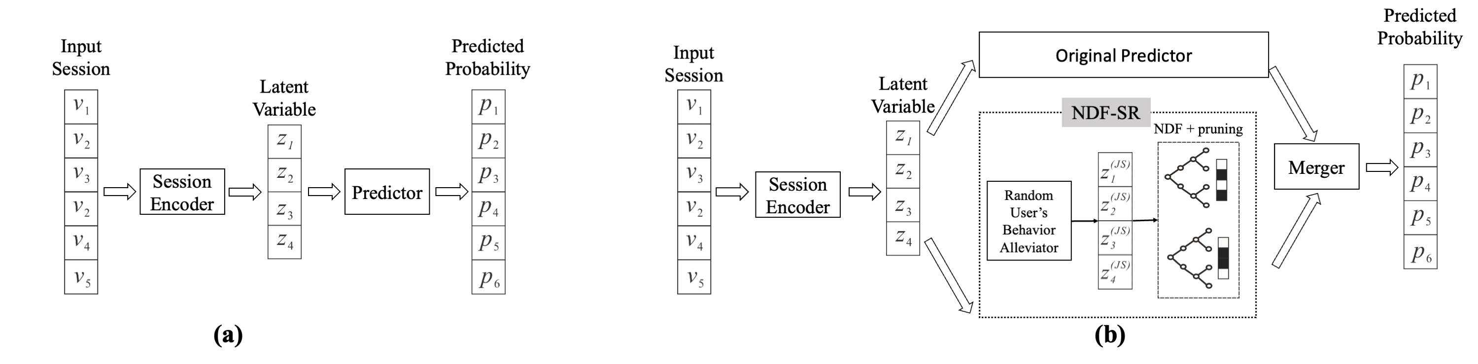
Figure 1: (a) The overview of the base model, (b) Framework SR-PredictAO; Given an input session $S$, the encoder module generates the latent variable $\bm{z}$. In (a), $\bm{z}$ is passed to the base model predictor module to obtain the predicted probability distribution over all items. In (b), $\bm{z}$ is passed to both the base model predictor module and the new predictor module (called NDF-SR) to obtain two predicted probability distributions over all items. Then, module Merger combines the two distributions to output the final distribution.

Due to the highly practical value in the field of modern commerce, the session-based recommendation attracts researchers’ interest. In recent years, most (if not all) proposed models followed the encoder-predictor paradigm, involving 2 components. The first component is the session encoder module, and the second component is the predictor module. The session encoder module transforms the input session (represented in the form of a sequence of items) into an $n^{\prime}$-dimensional vector called the latent variable, where $n^{\prime}$ is a positive integer denoting a model parameter. The predictor module generates a probability distribution over all items that represents how likely each item is to be the next item. The paradigm is shown in Fig. 1 (a). Different existing models have different implementations of the encoder modules. For example, in [2], the encoder module is a Gated GNN that captures complex transitions of items to obtain the latent variable, and in [3], the encoder module is a Star GNN that uses a star node, representing the whole session, and a Highway Network, handling the overfitting problem. The predictor modules of most (if not all) existing models are all linear models. Similar encoder-predictor paradigms could also be found in [4, 5, 6, 7, 8, 9].

Although existing models following the current encoder-predictor paradigm perform well, there are still some issues for further enhancement. The first issue is that most (if not all) existing models have a low-capability predictor module, which affects the prediction accuracy. Specifically, under the encoder-predictor paradigm, even though there is an advanced model in the encoder module constructing the latent variable (which could represent the latent intent of a user’s purchase), another important part in this recommendation comes from the predictor module, which could somehow simulate the complicated decision process of a human’s purchase. Unfortunately, most (if not all) existing models have linear models, which are low-capability models, limiting the prediction performance.

The second issue is that designing a high-capability model is challenging by considering the overfit problem. Specifically, one straightforward solution for the first issue is to design a high-capability model. It is well-known that an extremely high-capability model suffers from the overfit problem. How to design an appropriate high-capability model is needed for detailed investigation.

The third issue is that there is random user’s behavior in the input session, which may affect the prediction performance. Specifically, when a user browses some items, s/he normally has a clear intention on what s/he wants to view, but sometimes, the s/he may browse some other items that have little relation with his/her original intention due to his/her curiosity of seeing other items in a session. We call this kind of user’s behavior as random user’s behavior, which could create a challenge for prediction in existing models.

In this paper, we propose a novel framework called Session-based Recommendation with Predictor Add-On (SR-PredictAO). Under SR-PredictAO, given an existing model called the base model in this paper, we keep all existing modules of this existing model but we augment this model with two additional modules. The first additional module is the high-capability predictor module, which takes the latent variable as input and outputs the predicted probability distribution over all items being the next item in the session. Although we keep the original (low-capability) predictor module, we still include the new high-capability predictor module which could capture the complex human’s decision process. The second additional module is module Merger, which takes the probability distributions over all items predicted by both the original predictor module and the new predictor module and outputs the final probability distribution over all items. This framework provides a lot of opportunities to researchers for optimization on how to specify these 2 modules, which is quite promising. The SR-PredictAO framework could be found in Fig. 1 (b) where the first augmented module is named as NDF-SR (which will be described next). It is worth mentioning that our framework SR-PredictAO could be applied to all existing models following the encoder-predictor paradigm (with the two additional modules), which could further improve the prediction performance of all existing models.

In this paper, we propose a model called Neural Decision Forest for Session-based Recommendation (NDF-SR) for the first high-capability predictor module. Specifically, NDF-SR involves two components. The first component is called the random user’s behavior alleviator, which could minimize the effect of random user’s behaviors for the prediction process (addressing the third issue). The second component is called the Neural Decision Forest (NDF) model, which is a high-capability model (addressing the first issue). It could be regarded as a forest involving a number of decision trees each constructed with the use of neural network models. We also propose a pruning method in the NDF model to avoid the overfit problem (addressing the second issue). Furthermore, in this paper, for the second Merger module, we adopt a simple linear combination which combines the predicted distributions from the original predictor and the new predictor to obtain the final predicted probability distribution. In the following, for clarify, when we describe SR-PredictAO, we mean the framework adopting the above modules.

In summary, our contributions are shown as follows.

1. To the best of our knowledge, we are the first to find the important low-capability issue in the predictor module of most (if not all) existing models, lowering down their prediction accuracy.

2. To address this important issue, we propose a framework called SR-PredictAO including the high-capability predictor module where this module involves two components, namely the random user’s behavior alleviator (addressing the random user’s behavior issue) and the Neural Decision Forest (NDF) model (addressing the low-capability predictor issue). Moreover, we propose some pruning method in the NDF model to address the overfit problem.

3. We conduct extensive experiments on two public benchmark datasets, namely Yoochoose and Diginetica, for three state-of-the-art models. Experimental results show that SR-PredictAO improves almost all state-of-the-art models on all datasets up to 2.9% on HR@20 (one accuracy measurement) and up to 2.1% on MRR@20 (another accuracy measurement), which could set a new state-of-the-art in the literature. This improvement is consistent on all datasets. By considering the consistency of improvement and the ease of applicability of our framework, we regard our contribution as a major improvement to the field of the session-based recommendation system.

II Related Work

In this section, we give the related work about session-based recommendation (Section II-A) and neural decision forest (Section II-B).

II-A Session-based recommendation

We categories existing studies about session-based recommendation into three categories: (1) conventional recommendation methods, (2) neural-network-based methods and (3) graph neural-network-based methods.

Due to the similarity between the session-based recommendation (SR) problem and the traditional recommendation problem, conventional methods like Collaborative Filtering (CF) approaches [10, 11], nearest-neighbor approaches [12, 13] and Markov’s chain approaches [14] are applied to the SR problem. However, due to the limited information in the session, they all performed poorly in the SR problem.

With the improvement of computation power and knowledge in Neural Network (NN), many NN-based models, including RNN approaches [15], the transformer-based approach [16] and the CNN-based approach [17, 18], have been proposed. However, most of them do not perform well due to the limited information in the session.

In recent years, graph neural networks (GNNs) have become popular and have been shown to have state-of-the-art performance in many domains. Many recommendation systems [2, 5, 3, 6] also utilize GNNs due to its ability of modeling complex relationships among objects. In [2], Wu et al. apply gated graph neural networks (GGNNs) to capture the complex transitions of items, which result in accurate session representations. In [5], to solve information loss problems in GNN-based approaches for session-based recommendation, Chen et al. proposed a lossless encoding scheme, involving a dedicatedly designed aggregation layer and a shortcut graph attention layer. In [3], Pan et al. proposed Star Graph Neural Networks with Highway Networks (SGNN-HN) for session-based recommendation. In particular, the highway networks (HN) can select embeddings from item representations adaptively to order to prevent from overfitting. However, all aforementioned studies [2, 5, 3, 6] use a linear model, a low-capability model, as the predictor module (described in Section I).

II-B Tree-based method

The traditional tree-based method was proposed by Breiman in [19, 20]. Its outstanding performance in simulating the human decision process is studied by Quinlan et al. in [21] The high capability of the tree-based methods was shown by Mentch et al. [22]. With the rapid development of computation power and neural networks, a lot of effort has been made to combine classical tree-based methods with neural networks. In [23], Richmond et al. introduced Convolutional Neural Networks (CNNs) as representation learners on a traditional random forest. Jancsary et al. in [24] introduced regression tree fields for image restoration. To solve the problem that the traditional tree-based method cannot do backward propagation with other NN-based parts in the model, in [25], Kontschieder et al. constructed uniform and end-to-end differentiable Deep Neural Decision Forest and applied it to some computer vision models. To the best of our knowledge, no existing studies about session-based recommendation system utilizes the the tree-based models incorporated with the backward propagation with the NN-based parts in the models. We are the first one to propose this in the field of session-based recommendation system.

III Preliminaries

In this section, we introduce (1) problem definition (Section III-A), (2) some preliminary knowledge about a base model, an existing model, following the encoder-predictor paradigm (Section III-B) and (3) the traditional version of the tree-based method (Section  III-C).

III-A Problem Definition

The session-based recommendation is a sub-field of the next-item recommendation only with the input from a specific session. Its goal is to predict the next item that a user will browse based on the current active session involving all previus items browsed. We denote $I=\{v_{1},v_{2},\cdots,v_{N}\}$ by the universal set of items in the whole dataset, where $N$ is the total number of items. A session, denoted by $\bm{s}_{i}=[s_{i,1},s_{i,2},\cdots,s_{i,l_{i}}]$, is a time-ordered sequence of items, where $i$ is a temporary index of the session, $l_{i}$ denotes the length of $\bm{s}_{i}$ and, for each $t\in[1,l_{i}]$, $s_{i,t}\in I$ is the item at time step $t$ in the session. The goal of the session-based recommendation is to predict what the next item $s_{i,l_{i}+1}$ is. A typical session-based recommendation system generates a probability distribution over all items predicted being the next item, i.e., $\mathbb{P}(s_{i,l_{i}+1}|\bm{s}_{i})$.

III-B Base Model

The base model (following the encoder-predictor paradigm) is formulated as follows.

$$\bm{z}=f_{\textit{encode}}(\bm{s}|\Theta_{\textit{encoder}})$$ (1)

$$\bm{y}_{base}=g_{\textit{predict}}(\bm{z}|\Theta_{\textit{predictor}})$$ (2)

where (1) $\bm{s}$ is the input session (represented in the form of a sequence of items), (2) $\bm{z}$ is the latent variable generated by the encoder module of the model, (3) $\bm{y}_{base}$ denotes the probability distribution over all items predicted being the next item, (4) $f_{\textit{encode}}$ is the encoder which takes the input session as input and outputs a latent variable (a vector in $\mathbb{R}^{n^{\prime}}$) (5) $g_{\textit{predict}}$ is the predictor module which takes the latent variable as input and outputs the probability distribution, and (6) $\Theta_{\textit{encode}}$ ($\Theta_{\textit{predict}}$) is the parameter configuration of the encoder (predictor) module.

As described in Section I, different existing models have different implementations of the encoder modules. In the following, we describe the encoder module and the predictor module of a base model of some state-of-the-art models.

III-B1 Encoder Module

This section focuses on the most popular base model’s session encoding method, the GNNs encoder. But our methods can work on all kinds of session encoders as long as it generates a latent variable. GNNs are Neural Networks (NN) that directly operate on the graph of data, given a graph $G=(V,E)$, where each node $v_{i}\in V$ represents an item in $\bm{s}$ (the session). Typically, $v_{i}$ is associated with a node feature vector $\bm{x}_{i}$, which is the input to the first layer of GNNs. $\bm{x}_{i}\in\mathbb{R}^{n}$ is obtained by multiplying the embedding matrix (we define embedding matrix as $\bm{A}\in\mathbb{R}^{N\times n}$ with the item ID), where $n$ is the embedding dimensionality. And $\bm{A}$ is a trainable matrix. Assume we totally have $L$ layers of GNN. The formula of $l$-th ($l\leqslant L$) layer of GNN can be represented as follows:

$$\bm{x}_{i}^{(l+1)}=f^{(l)}(\bm{x}_{i}^{(l)},\bm{a}_{i}^{(l)})$$ (3)

$$\bm{a}_{i}^{(l)}=agg^{(l)}(\{msg^{(l)}(\bm{x}_{i}^{(l)},\bm{x}_{j}^{(l)})|(j,i)\in E_{in}(i)\})$$ (4)

where $\bm{x}_{i}^{(l)}$ is the embedding vector of node $i$ in the $l$-th layer of the GNN, and $E_{in}(i)$ is the set of incoming edges for node $v_{i}\in V$. The message processing function at the $l$-th layer $f^{(l)}$ generates the updated embedding of the target node based on its neighborhood. $agg^{(l)}$ is the aggregate function that connects the information of different edges together, and $msg^{(l)}$ is the message-extracting function that obtains information from the edge between $(x_{i}^{(l)},x_{j}^{(l)})$. Let $L$ be the total number of layers in the GNN. After $L$ steps of message passing, the final representation for the latent variable is:

$$\bm{h}_{G}=f_{out}(\{\bm{x}_{i}^{(L)}|v_{i}\in V\})$$ (5)

$\bm{h}_{G}$ is the graph-level representation that we regard as the graph latent variable generated by the readout function $f_{out}$.

After the graph level latent variable $\bm{h}_{G}$ is obtained, most models adds some additional information to obtain a better result. For example, [5] adds all results of the Embedding layer, EOPA Layer, and SGAT Layer’s (two special kinds of GNN mentioned in [5]) information to the graph representation, and [3] formulates the final result by concatenating $\bm{z}_{g}$ and $\bm{z}_{r}$, which are the last item’s representation and the combination of all the graphs’ result representation come from different levels respectively. After considering all the required information of the base model, we define this vector as the latent variable $\bm{z}\in\mathbb{R}^{n^{\prime}}$, where $n^{\prime}$ is the dimensionality of the latent variable. This approach is used in almost all well-known session-recommendation models [3, 6, 2, 5] .

III-B2 Predictor Module

After the encoder module outputs the latent variable, the predictor module takes this as input and performs the following steps.

1. The first step is to perform a prediction function (normally a linear model), which takes the latent variable as input and outputs an embedding called the session embedding $\bm{s}_{h}\in\mathbb{R}^{n}$ where $n$ is the dimensionality of the session embedding, same as the embedding dimension of $\bm{A}$

   $$\bm{s}_{h}=\text{Linear}(\bm{z})$$ (6)

2. The second step is to obtain the score vector $\bm{c}\in\mathbb{R}^{N}$ over all items predicted being the next item.

   $$\bm{c}=[c_{1},c_{2},\cdots,c_{N}]^{T}=\bm{A}\bm{s}_{h}$$ (7)

   where $c_{i}\in\mathbb{R}$ is a score of item $v_{i}$ predicted being the next item for each $i\in[1,N]$ and $\bm{A}\in\mathbb{R}^{N\times n}$ is the item embedding matrix we used before.

3. The third step is to obtain the probability vector $\hat{\bm{y}}_{base}\in\mathbb{R}^{N}$ over all items predicted being the next item by using the softmax function based on the score vector $\bm{c}$.

   $$\hat{\bm{y}}_{base}=softmax(\bm{c})=\frac{\exp(\bm{c})}{\sum_{i\in[1,N]}\exp(c_{i})}$$ (8)

III-C Tree-based method

From the mathematical point of view, the tree-based method is a way of generating a locally constant function, represented by function $tree:\mathbb{R}^{n^{\prime}}\rightarrow\mathbb{R}^{N}$ that divides the input space $\mathbb{R}^{n^{\prime}}$ into many regions, and give each subspace a constant value in $\mathbb{R}^{N}$. And we can define the tree recursively by first defining the tree-split function $\varphi$:

$$\varphi(\bm{x})=\chi(\bm{x}\in S)\bm{c}_{l}+\chi(\bm{x}\notin S)\bm{c}_{r}$$ (9)

where $S\subseteq\mathbb{R}^{n^{\prime}}$ is a subregion of the input space, and $\chi(\bm{x}\in S)$ is judging function that returns 1 when $x\in S$, and 0 otherwise. The $\bm{c}_{l},\bm{c}_{r}$ are defined as the left and right nodes of the tree-split. If $\bm{c}_{l}$ or $\bm{c}_{r}$ have its value in $\mathbb{R}^{N}$, where $N$ is the dimension of the predicted result, then we say it is a leaf node; if not, it is an internal node that is associated with another tree split $\varphi_{l/r}$. And the tree function can be represented as $tree(\bm{x})=\varphi_{root}(\bm{x})$ where $\varphi_{root}$ is the tree-split function associated with the root node, the beginning node of the tree. The max number of tree-split need to have from the root to the leaf node is defined as depth.

For example, in Fig. 2, each node $d_{i}(i\in[1,7])$ is associated with a tree split function $\varphi_{i}$ with corresponding region $S_{i}$. The node of $d_{1}$ is the root node (i,e., $tree=\varphi_{1}$), the nodes of $d_{i\neq 1}$ are internal nodes. And node of $\bm{\pi}_{j}(j\in[1,8])$ is leaf node that have its value $\bm{\pi}_{j}\in\mathbb{R}^{N}$.

IV Framework SR-PredictAO

Framework SR-PredictAO involves two modules, namely the high-capability predictor module (Section IV-A) and the Merger module (Section IV-B). The training process of SR-PredictAO is presented in Section IV-C.

IV-A High-Capability Predictor Module

We propose a model called Neural Decision Forest for Session-based Recommendation (NDF-SR) for the high-capability predictor module. Specifically, NDF-SR involves two components. The first component is called the random user’s behavior alleviator (Section IV-A1) and the second component is called the Neural Decision Forest (NDF) model (Section IV-A2). As described in Section I, we also propose a pruning method in the NDF model to avoid the overfit problem. This pruning method could be found in the description for the second component.

IV-A1 Random User’s Behavior Alleviator

The base-model encoded latent variable for the previous session view of items is normally heavily affected by random user’s behavior. To solve this problem, we could take the Empirical Bayes’ point of view [26]. For Empirical Bayes’, the observed data is not the underlying true value but a sample under a certain distribution around the truth. We would design our Alleviator under this cognition.

Formally, if a batch $\bm{Z}\in\mathbb{R}^{m\times n^{\prime}}$ of $m$ latent variables each with dimensionality of $n^{\prime}$ we observe from the base model’s encoder is:

$$\bm{Z}=\begin{bmatrix}\bm{z}_{1}^{T}\\ \bm{z}_{2}^{T}\\ \vdots\\ \bm{z}_{m}^{T}\end{bmatrix}=\begin{bmatrix}\bm{\xi}_{1}\\ \bm{\xi}_{2}\\ \vdots\\ \bm{\xi}_{n^{\prime}}\end{bmatrix}^{T}=\begin{bmatrix}z_{11}&z_{12}&\cdots&z_{1n^{\prime}}\\ z_{21}&z_{22}&\cdots&z_{2n^{\prime}}\\ \vdots&\vdots&\ddots&\vdots\\ z_{m1}&z_{m2}&\cdots&z_{mn^{\prime}}\end{bmatrix}$$

We denote $\bm{z}_{j}$ to be the $j$-th row of $\bm{Z}$ and also the latent variable of the $j$-th session in the batch for each $j\in[1,m]$. We denote $\bm{\xi}_{i}$ to be the $i$-th column of $\bm{Z}$ for each $i\in[1,n^{\prime}]$.

$\bm{Z}$ is not the underlying truth value for the latent variable but a sample from a distribution with the underlying truth value as its expected value. Suppose that $\bm{\mu}\in\mathbb{R}^{m\times n^{\prime}}$ denotes the correspondence truth values as follows.

$$\bm{\mu}=\begin{bmatrix}\mu_{11}&\mu_{12}&\cdots&\mu_{1n^{\prime}}\\ \mu_{21}&\mu_{22}&\cdots&\mu_{2n^{\prime}}\\ \vdots&\vdots&\ddots&\vdots\\ \mu_{m1}&\mu_{m2}&\cdots&\mu_{mn^{\prime}}\end{bmatrix}=\begin{bmatrix}\bm{\mu}_{1}^{T}\\ \bm{\mu}_{2}^{T}\\ \vdots\\ \bm{\mu}_{m}^{T}\end{bmatrix}$$

The Empirical Bayes’ assumption is that $\forall i,j;z_{ij}|\mu_{ij}\sim\mathcal{N}(\mu_{ij},\sigma_{j}^{2})$, which is a normal distribution with mean $\mu_{ij}$ and variance $\sigma_{j}^{2}$, with an additional assumption that $\sigma_{j}^{2}\geqslant 1$. This assumption also means that the variance is the same across different columns. We aim to obtain an estimator for $\bm{\mu}$ given the observation $\bm{Z}$. The Maximum Likelihood Estimator (MLE) that is commonly used in the field suggests that we should just take the $\bm{Z}$ itself. That is, for each $i\in[1,m]$ and each $j=[1,n^{\prime}]$,

$$\hat{\mu}_{ij}^{(MLE)}=z_{ij}$$ (10)

But, our alleviator uses the James-Stein Estimator for Session-based Recommendation (JSE-SR) that applies indirect evidence from other values of the same entry in the batch. The JSE-SR is defined as follows:

$$\hat{\mu}_{ij}^{(JS)}=(1-\frac{m-2}{\|\bm{\xi}_{j}\|^{2}})z_{ij}$$ (11)

For each of the two estimators $\hat{\mu}_{ij}$ (i.e.,$\hat{\mu}_{ij}^{(MLE)}$ and $\hat{\mu}_{ij}^{(JS)}$), the effect of random user’s behavior on the latent variable can be quantified as follows. For each $j\in[1,n^{\prime}]$, $\mathbb{E}[\sum_{i=1}^{m}(\mu_{ij}-\hat{\mu}_{ij})^{2}]$.

We can show the following lemma. In this lemma, we know that the estimator $\hat{\mu}_{ij}^{(JS)}$ gives a smaller error compared with the estimator $\hat{\mu}_{ij}^{(MLE)}$.

Lemma IV.1

$$\mathbb{E}[\sum_{i=1}^{m}(\mu_{ij}-\hat{\mu}^{(JS)}_{ij})^{2}]\leqslant\mathbb{E}[\sum_{i=1}^{m}(\mu_{ij}-\hat{\mu}^{(MLE)}_{ij})^{2}]$$ (12)

Proof Sketch: Firstly, for all predictor $\hat{\mu}_{ij}:=\hat{\mu}_{ij}(z_{ij})$ of $\mu_{ij}$, we can decompose $\mathbb{E}[\sum_{i=1}^{m}(\mu_{ij}-\hat{\mu_{ij}})^{2}]=\sum_{i=1}^{m}\mathbb{E}[(z_{ij}-\hat{\mu}_{ij})^{2}]+2\sum_{i=1}^{m}\mathbb{E}[(\hat{\mu}_{ij}-\mu_{ij})(z_{ij}-\mu_{ij})]$. Secondly, we perform integration by parts, we have: $\mathbb{E}[(z_{ij}-\mu_{ij})(\hat{\mu}_{ij}-\mu_{ij})]=\sigma_{j}^{2}\mathbb{E}[\frac{\partial\hat{\mu}_{ij}}{\partial z_{ij}}]$. Thirdly, we plug the $\hat{\mu}_{ij}^{(JS)}$ and $\hat{\mu}_{ij}^{(MLE)}$ into the equation, we have Equation 11. A complete proof could be found in Appendix--A.

Therefore, applying JSE-SR to all entries in $\bm{Z}$, we have:

$$\hat{\bm{Z}}^{(JS)}=[\hat{\mu}^{(JS)}_{ij}]_{i\in[1,m],j\in[1,n^{\prime}]}$$ (13)

IV-A2 Neural Decision Forest (NDF)

As described in Section I, the Neural Decision Forest (NDF) model could be regarded as a forest involving a number of decision trees each constructed with the use of neural network models. Each decision tree in this model is formally named as a neural decision tree (NDT).

In the following, we first define NDT and then NDF.

NDT: Our proposed NDT method is the part that provides (more than) enough capability to solve the lack of capability problem of the linear predictor. Considering the representation learning in the session-based recommendation, our proposed NDT differs from the traditional trees that greedily find the split that may reduce the loss function in the given variable space and entries proposed by [19], which requires a fixed encoder, but our proposed NDT uses Neural Networks (NN) to do the split and are optimized by backward propagation together with the encoder. In our case, this encoder is normally a GNN-based encoder. The NDT that has depth $d$, and it takes values from alleviator-processed latent variable $\bm{z}^{(JS)}\in\mathbb{R}^{n^{\prime}}$ as input. It consists of the following.

• A decision function (normally a deep neural network): $f:\mathbb{R}^{n^{\prime}}\rightarrow\mathbb{R}^{2^{d}-1}$ (because a tree with depth $d$ requires $2^{d}-1$ number of the split, resulting in $2^{d}$ leaf nodes)

• A probability score matrix $\bm{\pi}\in\mathbb{R}^{2^{d}\times N}$ (which is trainable) for all leaf nodes:

  $$\bm{\pi}=[\pi_{ij}]=[\bm{\pi}_{1},\cdots,\bm{\pi}_{2^{d}}]^{T}$$ (14)

  We mark the leaf nodes of a tree from left to right with index $1,2,\cdots,2^{d}$, where the $i$-th leaf node means the leaf node with index $i$. Note that under our definition, the NDT is always a balanced tree. $\pi_{ij}$ means the probability score of the $j$-th item in the $i$-th leaf node. $\bm{\pi}_{i}$ means a vector containing the probability scores of all items in $I$ of the $i$-th leaf node.

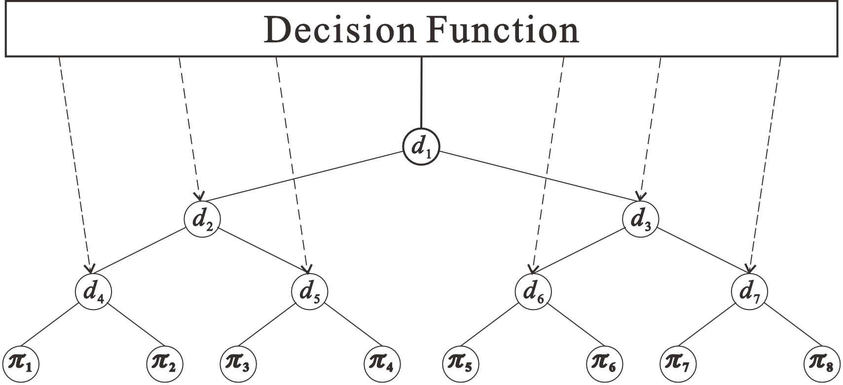
Figure 2: The overview of the NDT, decision function gives the split score for root and internal nodes, and the leaves nodes’ result is the probability of the session reaching the node

The NDT works as follows. The decision function generates a decision score for each split. Then, applying a sigmoid function to the decision score to obtain the right and left decision probability. A binary split is associated with the probability of arriving at the root of this split as $p_{root}$, which is generated by previous splits. Let $s=\sigma(f(z^{(JS)}))$. The split here means the process of giving an item in the root of the subtree what is the probability that this item goes to the right and left of the root. The probability is calculated as follows.

$$\begin{cases}p_{left}=p_{root}\cdot s\\ p_{right}=p_{root}\cdot(1-s)\end{cases}$$ (15)

For example, in Fig. 2, $p_{root}$ for node $d_{1}$ is 1, and $p_{root}$ for node $d_{2}$ is set to $p_{left}$ computed within node $d_{1}$.

We recursively apply this split method from the tree’s root to the leaf nodes. We obtain the leaf-reaching probability $\bm{p}_{leaf}=[p_{1}^{(leaf)},p_{2}^{(leaf)},\cdots,p_{2^{d}}^{(leaf)}]^{T}\in\mathbb{R}^{2^{d}}$ to represent what is the probability that this session may fall into each leaf node. Then, multiply $softmax(\bm{\pi})$ matrix by $\bm{p}_{leaf}$ to obtain the probability distribution $\hat{\bm{p}}\in\mathbb{R}^{N}$ over all items that this session may represent.

$$\hat{\bm{p}}=\bm{p}_{leaf}^{T}softmax(\bm{\pi})=\sum_{k=1}^{2^{d}}p_{k}^{(leaf)}softmax(\bm{\pi}_{k})$$ (16)

where $\hat{\bm{p}}$ is the predicted probability for each item for this tree. To make $\bm{\pi}$ normalized, we apply the softmax function before we use it.

Pruning: Because that all tree-based methods, including NDT, suffer from serious overfitting because they normally have excessive capability. The problem is more severe in our case since our NDT is trained simultaneously with the encoder. To solve that problem, we propose NDT-pruning that can control the excessive capability to control overfitting.

Traditional pruning uses the judgment of loss function to see which leaves should drop, but for an NDT, it is hard to do a similar thing. Thus, to prune the NDT, we apply a random mask to the outcomes of NDT. So we do the following:

$$\bm{p}^{\prime}_{leaf}=softmax(RandomMask(\bm{p}_{leaf},r))$$ (17)

where $\bm{p}_{leaf}\in\mathbb{R}^{2^{d}}$ is the leaf-reaching probability, and each leaf node has a probability $r$ (we call it pruning rate) to be 0, and $r\in[0,1]$. After the random mask, we use $\bm{p}^{\prime}_{leaf}$ to replace $\bm{p}_{leaf}$ to obtain $\hat{\bm{p}}$, the predicted next-item distribution of this tree.

Since the NDT typically has excessive capability than needed, which may fit into unrelated information in data, this makes the model easy to overfit. Our proposed NDT-pruning controls the overfitting by removing the excessive capability of the NDT. By choosing a good pruning rate, we can control the capability of our model in a reasonable range that can compensate for the lack of capability in linear predictors and not be too high to overfit. More details of the relation between the model’s capability and NDT-pruning can be found in the technique report in the git repository

NDF: We construct the NDF by the basic building block NDT and NDT-pruning in this section. Breiman proved that combining trees into a forest model generally makes the model’s outcome more stable [20]. Non-neural trees that formulate Random Forest should have a different mask of entries for every split, but that is not possible if we use a uniform decision function for each tree. So, we independently drop some entries for each NDT.

For example, if an input Alleviator-processed latent variable for the NDT is $\bm{z}^{(JS)}=[z_{1}^{(JS)}\cdots,z_{n^{\prime}}^{(JS)}]^{T}\in\mathbb{R}^{n^{\prime}}$ , for the $i$-th NDT after the variable mask-off, a fixed subset of $\bm{z^{\prime}}_{i}=[z_{1_{i}},z_{2_{i}},\cdots,z_{\gamma_{i}}]$ where $|\bm{z}_{i}^{\prime}|=\gamma_{i}\leqslant n^{\prime}$, and $\bm{z^{\prime}}\subseteq\bm{z}^{(JS)}$. For each NDT, the list of entries to drop is randomly selected when building the model, but this list is fixed during training. If there are $T$ number of NDTs in the NDF-SR, and their predicted next-item probability is $\bm{P}=[\hat{\bm{p}}_{1},\hat{\bm{p}}_{2},\cdots,\hat{\bm{p}}_{T}]$, where $\hat{\bm{p}}_{i}\in\mathbb{R}^{N}$ for all $i=1,2,\cdots,T$. The NDF’s predicted result is:

$$\hat{\bm{y}}_{NDF-SR}=\frac{1}{T}\cdot(\sum_{i=1}^{T}\hat{\bm{p}}_{i})$$ (18)

which is also the predicted result of the NDF-SR, our proposed high-capability predictor.

We can prove by simulated data that, typically, the NDF-SR has a much higher capacity than the linear predictor. More details are in the technique report in the git repository.

IV-B Merger Module

In this paper, for the second Merger module, we adopt a simple linear combination which combines the predicted distributions from the original predictor and the new predictor to obtain the final predicted probability distribution by using a user parameter $q\in[0,1]$ as follows.

$$\hat{\bm{y}}=q\cdot\hat{\bm{y}}_{base}+(1-q)\cdot\hat{\bm{y}}_{NDF-SR}$$ (19)

Here, $\hat{\bm{y}}\in\mathbb{R}^{N}$ is the probability distribution over all items predicted being the next item (which is the combined result from the original predictor module and the new predictor module). $\hat{\bm{y}}$ is the output of framework SR-PredAO.

IV-C Training

Note that $\hat{\bm{y}}$ obtained in module Merger is the output of framework SR-PredAO. Let $\bm{y}$ be the real probability distribution over all items being the next item, which is a one-hot vector. The loss function of framework SR-PredAO $\mathcal{L}(\cdot,\cdot)$ is the same as the one used in the base model, which is the cross-entropy loss.

$$\mathcal{L}(\bm{y},\hat{\bm{y}})=-\bm{y}^{T}\log(\hat{\bm{y}})$$ (20)

For initialization, all trainable parameters in both the base model and the additional modules in framework SR-PredAO are initialized randomly, and they are jointly updated in an end-to-end back propagation manner.

V Experiment

We give the experimental setup in Section V-A and the experimental results in Section V-B. Implementation of this paper can be found in this link ( https://github.com/RickySkywalker/SR-PredictAO-official ).

V-A Experimental Setup

V-A1 Datasets

We evaluated the performance of state-of-the-art models and our proposed framework on the following two benchmark real-world datasets:

• Yoochoose is a dataset obtained from the RecSys Challange 2015, which contains user sessions of click events from an online retailer.

• Diginetica is a dataset released by the CIKM Cup 2016, which includes user sessions extracted from e-commerce search engine logs.

Following [3, 5], for both datasets, we first filter out short sessions and infrequent items so that only sessions of length at least 2 and items that appear at least 5 times are kept. We split the training set and the test set in the following way. For Yoochoose, we use the sessions on the last day as the test set, and for Diginetica, we use the sessions of the last week as the test set. In particular, since Yoochoose is too large, we only use the recent 1/64 fraction of the training set to train our model, denoted as Yoochoose 1/64. We also tried to use Yoochoose 1/4 (denoting the recent 1/4 fraction) for testing the performance of models on datasets with different scales, but it turns out the dataset is too large and our computation power cannot support this dataset.

Moreover, following [3, 16], we utilize the sequence splitting to preprocess datasets. Specifically, for an input session, $[v_{1},v_{2},...,v_{n}]$, we generate the sequences and the corresponding labels as $([v_{1}],v_{2})$, $([v_{1},v_{2}],v_{3})$,…,$([v_{1},v_{2},...,v_{n-1}],v_{n})$ for training and testing. The statistics of the datasets after pre-processing are provided in Table I.

Statistic	Yoochoose 1/64	Diginetica
# of Clicks	$565332$	$982961$
# of Training Sessions	$375625$	$647523$
# of Test Sessions	$55896$	$71947$
# of Items	$17792$	$43097$
Average length	6.14	5.12

TABLE I: Statistics of datasets

V-A2 Evaluation Metrics

Following previous studies [27, 28, 2, 29, 5, 3, 4, 6], we adopt the commonly used HR@20 (Hit Rate) and MRR@20 (Mean Reciprocal Rank) as our evaluation metrics.

V-A3 Base Model

Framework SR-PredAO involves a base model (together with our proposed high-capabitliy predictor module andn the Merger module). In our experiments, we choose the following three base models, namely LESSR [5], SGNN-HN [3] and DIDN [6], since they are representative in the literature. Roughly speaking, LESSR has a clear encoder-predictor paradigm for the ease of illlustration. SGNN-HN and DIDN have the best performance on datasets Yoochoose 1/64 and Diginetica, respectively.

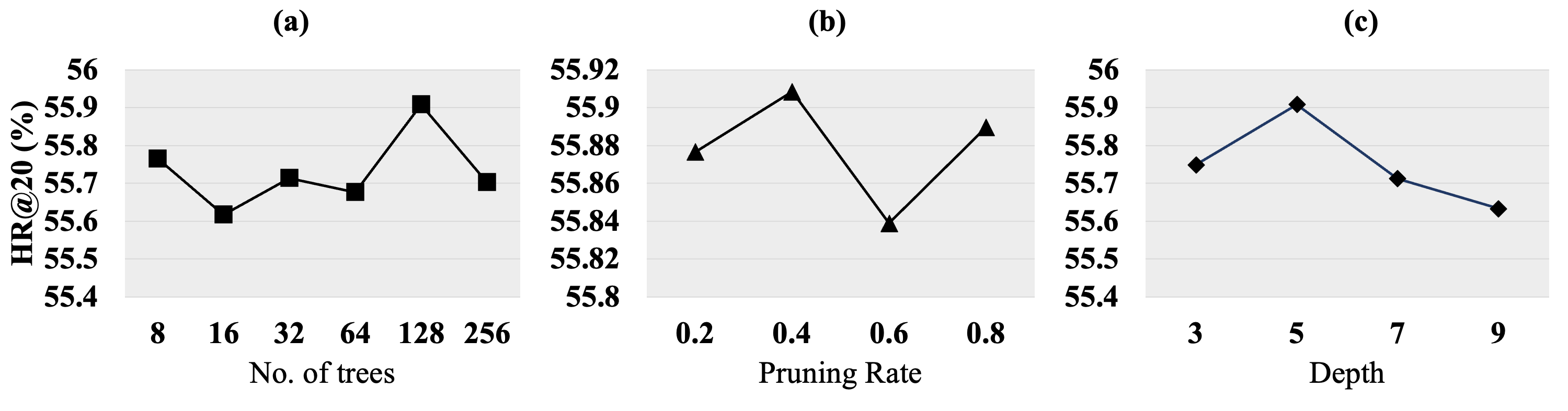
Figure 3: The hyper-parameter study results of SR-PredAO(SGNN-HN)

• LESSR [5]: LESSR, proposed by Chen et al. in 2020, intends to solve the lossy session encoding problem from the classical model of SR-GNN [2]. We chose this model as one of the base models because it has the clear encoder-predictor paradigm both in the paper and in the publicly-available code.

• SGNN-HN [3]: SGNN-HN, proposed by Pan et al. in 2020, introduces a star graph neural network to capture complex transition relationships among items in an on-going session and applies a highway network to deal with the over-fitting problem in existing GNNs. To the best of our knowledge, SGNN-HN is the state-of-the-art model in Yoochoose 1/64 from 2020 to 2023 because it has the best HR@20 as 72.06%, showing that it outperforms other models by around 1% according to https://paperswithcode.com/sota/session-based-recommendations-on-yoochoose1-1 . However, this model has an unclear encoder-predictor split in the paradigm, which affects the performance enhancement of SR-PredAD using this model as a base model.

• DIDN [6]: The DIDN, proposed by ZHANG et al. in 2022, offers a dynamic intent-aware model, solving the dynamic change of the user behaviors within the session, and an iterative de-noising model, filtering out noisy clicks within a session explicitly. It also further mines collaborative information to enrich the session semantics. To the best of our knowledge, the DIDN model is the state-of-the-art model in Diginetica. It outperforms other models in Diginetica dataset for at least 0.98% in HR@20 and 4.76% in MRR@20 according to https://paperswithcode.com/sota/session-based-recommendations-on-diginetica (Note: the DIDN model’s result could not be found in this link but its HR@20 and its MRR@20 are 56.22% and 20.02%, respectively).

We also considered using some newer proposed models like [7, 8, 9]. But, they do not have a state-of-the-art performance in these two datasets.

In the following, when we describe framework SR-PredAO using the base model $M$, we write SR-PredAO(M).

V-B Experimental Results

V-B1 Performance Comparison

Method	Diginetica		Yoochoose 1/64
	HR@20	MRR@20	HR@20	MRR@20
LESSR	51.71	18.15	70.94	31.16
SR-PredAO(LESSR)	53.10	18.38	71.73	31.70
Improvement (%)	2.7	1.3	1.1	1.7
SGNN-HN	55.67	19.12	72.06	32.61
SR-PredAO(SGNN-HN)	55.91	19.06	72.62	32.47
Improvement (%)	0.4	-0.3	0.8	-0.4
DIDN	56.22	20.03	68.95	31.27
SR-PredAO(DIDN)	57.86	20.49	69.50	31.44
Improvement (%)	2.9	2.3	0.8	0.5

TABLE II: Experimental result (%) on three base models and two datasets

In framework SR-PredAO, all hyper-parameters (e.g., the batch size and the learning rate) in the base models are kept as the best experimental configuration shown in the existing papers because we want to see the improvement of framework SR-PredAO (including the new predictor module and the merger module) on the base model.

Table II shows the experimental results of all models. Note that each reported result in the table is the best result of our model, and they may be in different parameter configurations.

From Table II, we see that framework SR-PredAO has a relatively significant improvement on HR@20 for all models and on MRR@20 for almost all models. Specifically, framework SR-PredAO, when applied to existing state-of-the-art models, could have up to 2.9% improvement on HR@20 and 2.3% of improvement on MRR@20. The improvement is on a considerably significant scale. Besides, when there is a clearer encoder-predictor paradigm in an existing model, the performance enhancement is more substantial. However, if the model does not have a clear split of the encoder module and the predictor module in its implementation, then there is no improvement on MRR@20.

It is worth mentioning that using framework SR-PredAO on any existing model could automatically improve the prediction accuracy, which is a great advantage. Compared with recent papers [5, 3, 6, 7, 8, 9, 4] showing that 1.4% of improvement is considered as a major contribution, framework SR-PredAO has a significant improvement in the field.

V-B2 Ablation Studies

In the following experimental results, all the experiments are conducted on the base model of SGNN-HN since the SGNN-HN is the most challenging model to be tuned for framework SR-PredAO. The experiment for this model can better reflect the effectiveness of each feature in framework SR-PredAO. We study two features, namely (1) the random user’s behavior alleviator and (2) NDT-pruning, by comparing the performance of SR-PredAO(SGNN-HN) with its model with one of the features removed.

Data Set	SR-PredAO(SGNN-HN)	Remove Alleviator	Remove Pruning
Diginetica	55.91	55.79	55.78
YC 1/64	72.62	72.58	72.58

TABLE III: Ablation test results (%) on random user’s behavior alleviator (Alleviator) and NDT-pruning (Pruning)

Table III shows that if we drop the random user’s behavior alleviator or NDT-Pruning in framework SR-PredAO, the improvement of SR-PredAO over the base model drops to a great extent in the Diginetica dataset but not that much in YooChoose (YC) 1/64 dataset. This is because the random user’s behavior and the overfitting problem are not quite obvious in the YC dataset compared with the Diginetica dataset.

V-B3 Hyper-parameter Study

In this section, we study how the number of trees, the depth of the tree, and the pruning rate affect the performance of SR-PredAO. All the results are shown in Fig. 3. When the number of trees reaches 128, HR@20 of SR-PredAO is the highest. When the number of trees is larger 128, HR@20 decreases because more trees affects the model’s learning capacity. For the pruning rate, as long as we do not remove the pruning feature, we can see that varying the rate does not affect the performance too much. For the depth of the tree, we can see that if the tree goes too deep (i.e., the depth is greater than 5), it may have a serious overfit problem due to the excessive capability, and if the tree is too shallow (i.e., the depth is smaller than 5), it cannot provide enough capability enhancement for prediction.

V-B4 Model Size Comparison

In order to perform a fair comparison between the base model (without using our framework) and our framework, we conduct experiments so that they have the same model complexities. Specifically, after we obtain SR-PredAO(SGNN-HN), we enlarge the base model (i.e., SGNN-HN) by increasing the embedding dimensionality and this base model (without using our framework), after parameter-tuning, is regarded as a baseline. The experimental result on Diginetica is shown in Table IV. The enlarged base model cannot outperform SR-PredAO(SGNN-HN) due to the inappropriate training capacity increment of the base model.

Model	Size	HR@20	MRR@20
Enlarged SGNN-HN	$1605$MB	55.24	18.64
SR-PredAO(SGNN-HN)	$1118$MB	55.91	18.78

TABLE IV: Size comparison (%) result on Diginetica

V-B5 Experimental Summary

In summary, framework SR-PredAO, when applied to existing state-of-the-art models, could have up to 2.9% improvement on HR@20 and 2.3% of improvement on MRR@20. We can observe this improvement in almost all base models on all datasets. By considering the consistency of improvement and the ease of applicability of our framework, we regard our contribution as a major improvement to the field of the session-based recommendation system.

VI Conclusion

In this paper, we are the first to discover the important low-capability issue in the predictor module of most (if not all) existing models, lowering down their prediction accuracy. To address this important issue, we propose a framework called SR-PredictAO which could be applied to any existing models following the common encoder-predictor paradigm. Extensive experimental results on two public benchmark datasets show that when framework SR-PredictAO is applied to 3 existing state-of-the-art models, their performance are consistently improved up to 2.9% on HR@20 and up to 2.1% on MRR@20. Due to the consistent improvement on all datasets, we regard our contribution as a major improvement to the field of the session-based recommendation system.

-A Proof of Alleviator

-A1 Assumption 1

All session data are i.i.d. (i.e., independent and identically distributed) samples affected by random user’s behavior under some uniform distribution $\mathbb{P}_{\textbf{s}}$.

i.e. For a set of collected sampled sessions: $\{\bm{s}_{i}\}_{i=1}^{m}$, where $\bm{s}_{i}=[s_{i,1},s_{i,2},\cdots,s_{i,l_{i}}]$ as we defined in Section III-A. For all $i$, we have: $\bm{s}_{i}-\epsilon_{i}\sim\mathbb{P}_{s}$ where $\epsilon_{i}$ is the random user’s behavior, which can be intuitively understood as the user’s random behavior

-A2 Assumption 2 (Empirical Bayes Assumption I)

The encoded value of a session (i.e., $z_{ij}$ in Section IV-A1) is not the real value, just an observation affected by random user’s behavior:

i.e., for a not affected session $\bm{s}_{i}-\epsilon_{i}$; the real encoded latent variable is $\bm{\mu}_{i}=[\mu_{i1},\cdots,\mu_{in^{\prime}}]^{T}$ ; For a fixed $j=1,2,\cdots,n^{\prime}$ (where $n^{\prime}$ is the dim for latent variable), the $\{\mu_{ij}\}_{i=1}^{m}$ and follows distribution $\mathbb{P}_{s}^{(j)}$.

That means the real value for $j-th$ propriety of the $i-th$ session should be $\mu_{ij}$; But due to the effect of random user’s behavior, the encoded result we observe from the session-encoder is $z_{ij}$

-A3 Assumption 3 (Empirical Bayes Assumption II)

The observed value of the encoded session $z_{ij}$ follows the distribution of $\mathcal{N}(\mu_{ij},\sigma_{j}^{2})$ and $\sigma_{j}\geqslant 1$ (if this assumption is not met, we can always do batch normalization to make the $\sigma_{j}$ not far from 1).

The Normal distribution assumption comes from the statistic common that if a distribution is affected by extremely complex factors, like the random user’s behavior. The safest way is to assume that they are normally distributed. Since all numbers in $\{z_{ij}\}_{i=1}^{m}$ represent the same factor of the session (the $j-th$ encoded factor), it is reasonable to assume they have the same and relatively large variance.

-A4 Target

In high-level understanding, what we observed in the real data is not the full fact but noisy data that have information of the underlying true value. Our goal is to obtain the underlying true value (i.e., $\mu_{ij}$ in our case) through observed values (the $z_{ij}$ in our case).

The rigorous definition of the target is: given a batched, observed encoded result: $\bm{Z}\in\mathbb{R}^{m\times n^{\prime}}$ and its corresponding underlying true value $\bm{\mu}\in\mathbb{R}^{m\times n^{\prime}}$

For a fixed $j\in[1,n^{\prime}]$, get an estimator $\hat{\mu}_{ij}|\bm{\xi}_{j}$ for $\mu_{ij}$ s.t. $\mathbb{E}[\sum_{i=1}^{m}(\hat{\mu}_{ij}-\mu_{ij})^{2}]$ is small.

Consider the Max likelihood estimator $\hat{\mu}_{ij}^{(MLE)}=z_{ij}$, and $\hat{\mu}^{ij}_{(JS)}=(1-\frac{m-2}{\|\bm{\xi}_{j}\|^{2}})z_{ij}$.

Claim that: $\mathbb{E}[\sum_{i=1}^{m}(\mu_{ij}-\hat{\mu}_{ij}^{(JS)})^{2}]\leqslant\mathbb{E}[\sum_{i=1}^{m}(\mu_{ij}-\hat{\mu}_{ij}^{(MLE)})^{2}]$

-A5 Proof of claim

$\mathbb{E}[\sum_{i=1}^{m}(\mu_{ij}-\hat{\mu}_{ij})^{2}]=\sum_{i=1}^{m}\mathbb{E}[(z_{ij}-\hat{\mu}_{ij})^{2}-(z_{ij}-\mu_{ij})^{2}+2(\hat{\mu}_{ij}-\mu_{ij})(z_{ij}-\mu_{ij})]=\sum_{i=1}^{m}\mathbb{E}[(z_{ij}-\hat{\mu}_{ij})^{2}]-m\cdot\sigma_{j}+2\sum_{i=1}^{m}\mathbb{E}[(\hat{\mu}_{ij}-\mu_{ij})(z_{ij}-\mu_{ij})]$

Consider distribution function for $z_{ij}$ as: $\varphi(z_{ij}|\mu_{ij},\sigma_{j})=\frac{1}{\sqrt{2\pi}\cdot\sigma_{j}}\exp(-\frac{(z_{ij}-\mu_{ij})^{2}}{2\sigma^{2}_{j}})$. Therefore, $(z_{ij}-\mu_{ij})(\hat{\mu}_{ij}-\mu_{ij})=-\sigma_{j}^{2}\frac{\partial}{\partial z_{ij}}\varphi(z_{ij}|\mu_{ij},\sigma_{j})$

Therefore, for any continuous, differentiable, and $|f(z)|<\infty$, function $f:\mathbb{R}\rightarrow\mathbb{R}$. For simplicity, denote $\varphi(z_{ij}|\mu_{ij},\sigma_{j})$ as $\varphi(z_{ij})$ we have:

$$\mathbb{E}[(z_{ij}-\mu_{ij})f(z_{ij})]$$

$$= \int_{-\infty}^{+\infty}(z_{ij}-\mu_{ij})f(z_{ij})\varphi(z_{ij})dz_{ij}$$

$$= (-\sigma_{j}^{2})\cdot(\int_{-\infty}^{+\infty}(\frac{\partial}{\partial z_{ij}}\varphi(z_{ij}))f(z_{ij})dz_{ij})$$

$$= (-\sigma_{j}^{2})\cdot\varphi(z_{ij})\cdot f(z_{ij})|^{+\infty}_{-\infty}-\int_{-\infty}^{+\infty}f^{\prime}(z_{ij})\varphi(z_{ij})dz_{ij}$$

$$= \sigma_{j}^{2}\cdot(\int_{-\infty}^{+\infty}f^{\prime}(z_{ij})\varphi(z_{ij})dz_{ij})$$

$$= \sigma_{j}^{2}\mathbb{E}[\frac{\partial}{\partial z_{ij}}f(z_{ij})]$$

Therefore, we have: $\mathbb{E}[(z_{ij}-\mu_{ij})(\hat{\mu}_{ij}-\mu_{ij})]=\mathbb{E}[\frac{\partial\hat{\mu}_{ij}}{\partial z_{ij}}]\cdot\sigma_{j}^{2}$. Therefore, when $\hat{\mu}_{ij}$ is MLE: $\mathbb{E}[\sum_{i=1}^{m}(\mu_{ij}-\hat{\mu}_{ij}^{(MLE)})^{2}]=0-m\cdot\sigma_{j}^{2}+2m\cdot\sigma_{j}^{2}=m\cdot\sigma_{j}^{2}$ When $\hat{\mu}_{ij}$ is $\hat{\mu}_{ij}^{(JS)}$. We have: $\mathbb{E}[\frac{\partial\hat{\mu}_{ij}^{(JS)}}{\partial z_{ij}}]=1-\frac{m-2}{\|\bm{\xi}_{j}\|^{2}}+\frac{2(m-2)z_{ij}^{2}}{\|\bm{\xi}_{j}\|^{4}}$

Therefore, $\sum_{i=1}^{m}\mathbb{E}[(\hat{\mu}_{ij}^{(JS)}-\mu_{ij})(z_{ij}-\mu_{ij})]=m-\mathbb{E}[\frac{(m-2)^{2}}{\|\bm{\xi}_{j}\|^{2}}]$

With $\mathbb{E}[(z_{ij}-\hat{\mu}^{(JS)}_{ij})^{2}]=\mathbb{E}[\frac{(m-2)^{2}}{\|\bm{\xi}_{j}\|^{2}}z_{ij}^{2}]$, we have: $\mathbb{E}[\sum_{i=1}^{m}(\mu_{ij}-\hat{\mu}_{ij}^{(JS)})^{2}]=m\cdot\sigma_{j}^{2}+m(1-2\sigma_{j}^{2})\mathbb{E}[\frac{(m-2)^{2}}{\|\bm{\xi}_{j}\|^{2}}]$

Since in our assumption $\sigma_{j}^{2}\geqslant 1$, we have:

$$\mathbb{E}[\sum_{i=1}^{m}(\mu_{ij}-\hat{\mu}_{ij}^{(JS)})^{2}]\leqslant\mathbb{E}[\sum_{i=1}^{m}(\mu_{ij}-\hat{\mu}_{ij}^{(MLE)})^{2}]$$ (21)

References

- [1] J. Davidson, B. Liebald, J. Liu, P. Nandy, T. V. Vleet, U. Gargi, S. Gupta, Y. He, M. Lambert, B. Livingston, and D. Sampath, “The youtube video recommendation system,” in RecSys, 2010, pp. 293–296.
- [2] S. Wu, Y. Tang, Y. Zhu, L. Wang, X. Xie, and T. Tan, “Session-based recommendation with graph neural network,” in AAAI, 2019, pp. 346–353.
- [3] Z. Pan, F. Cai, W. Chen, H. Chen, and M. de Rijke, “Star graph neural networks for session-based recommendation,” in Proceedings of the 29th ACM international conference on information & knowledge management, 2020, pp. 1195–1204.
- [4] Y. Zheng, S. Liu, Z. Li, and S. Wu, “Dgtn: Dual-channel graph transition network for session-based recommendation,” in 2020 International Conference on Data Mining Workshops (ICDMW). IEEE, 2020, pp. 236–242.
- [5] T. Chen and R. C.-W. Wong, “Handling information loss of graph neural networks for session-based recommendation,” in Proceedings of the 26th ACM SIGKDD International Conference on Knowledge Discovery & Data Mining, 2020, pp. 1172–1180.
- [6] X. Zhang, H. Lin, B. Xu, C. Li, Y. Lin, H. Liu, and F. Ma, “Dynamic intent-aware iterative denoising network for session-based recommendation,” Information Processing & Management, vol. 59, no. 3, p. 102936, 2022.
- [7] R. Yeganegi and S. Haratizadeh, “Star: A session-based time-aware recommender system,” arXiv preprint arXiv:2211.06394, 2022.
- [8] P. Zhang, J. Guo, C. Li, Y. Xie, J. B. Kim, Y. Zhang, X. Xie, H. Wang, and S. Kim, “Efficiently leveraging multi-level user intent for session-based recommendation via atten-mixer network,” in Proceedings of the Sixteenth ACM International Conference on Web Search and Data Mining, 2023, pp. 168–176.
- [9] Z. Pan, F. Cai, W. Chen, C. Chen, and H. Chen, “Collaborative graph learning for session-based recommendation,” ACM Transactions on Information Systems (TOIS), vol. 40, no. 4, pp. 1–26, 2022.
- [10] A. Mnih and R. R. Salakhutdinov, “Probabilistic matrix factorization,” Advances in neural information processing systems, vol. 20, 2007.
- [11] Y. Koren and R. Bell, “Advances in collaborative filtering. recommender systems handbook, francesco ricci, lior rokach, bracha shapira, paul b. kantor editors, chapter 5,” 2011.
- [12] J. Davidson, B. Liebald, J. Liu, P. Nandy, T. Van Vleet, U. Gargi, S. Gupta, Y. He, M. Lambert, B. Livingston et al., “The youtube video recommendation system,” in Proceedings of the fourth ACM conference on Recommender systems, 2010, pp. 293–296.
- [13] S. E. Park, S. Lee, and S.-g. Lee, “Session-based collaborative filtering for predicting the next song,” in 2011 First ACIS/JNU International Conference on Computers, Networks, Systems and Industrial Engineering. IEEE, 2011, pp. 353–358.
- [14] S. Rendle, C. Freudenthaler, and L. Schmidt-Thieme, “Factorizing personalized markov chains for next-basket recommendation,” in Proceedings of the 19th international conference on World wide web, 2010, pp. 811–820.
- [15] B. Hidasi, A. Karatzoglou, L. Baltrunas, and D. Tikk, “Session-based recommendations with recurrent neural networks,” arXiv preprint arXiv:1511.06939, 2015.
- [16] J. Li, P. Ren, Z. Chen, Z. Ren, T. Lian, and J. Ma, “Neural attentive session-based recommendation,” in Proceedings of the 2017 ACM on Conference on Information and Knowledge Management, 2017, pp. 1419–1428.
- [17] T. X. Tuan and T. M. Phuong, “3d convolutional networks for session-based recommendation with content features,” in Proceedings of the eleventh ACM conference on recommender systems, 2017, pp. 138–146.
- [18] F. Yuan, A. Karatzoglou, I. Arapakis, J. M. Jose, and X. He, “A simple convolutional generative network for next item recommendation,” in Proceedings of the twelfth ACM international conference on web search and data mining, 2019, pp. 582–590.
- [19] L. Breiman, J. H. Friedman, R. A. Olshen, and C. J. Stone, Classification and regression trees. Routledge, 2017.
- [20] L. Breiman, “Random forests,” Machine learning, vol. 45, pp. 5–32, 2001.
- [21] J. R. Quinlan, “Decision trees and decision-making,” IEEE Transactions on Systems, Man, and Cybernetics, vol. 20, no. 2, pp. 339–346, 1990.
- [22] L. Mentch and S. Zhou, “Randomization as regularization: A degrees of freedom explanation for random forest success,” 2020.
- [23] D. Richmond, D. Kainmueller, M. Y. Yang, E. Myers, and C. Rother, “Relating cascaded random forests to deep convolutional neural networks for semantic segmentation,” 07 2015.
- [24] J. Jancsary, S. Nowozin, and C. Rother, “Loss-specific training of non-parametric image restoration models: A new state of the art,” in European Conference on Computer Vision. Springer, 2012, pp. 112–125.
- [25] P. Kontschieder, M. Fiterau, A. Criminisi, and S. R. Bulò, “Deep neural decision forests,” in 2015 IEEE International Conference on Computer Vision (ICCV), 2015, pp. 1467–1475.
- [26] C. Stein, “Variate normal distribution,” in Proceedings of the Third Berkeley Symposium on Mathematical Statistics and Probability: Contributions to the Theory of Statistics, vol. 1. University of California Press, 1956, p. 197.
- [27] J. Li, P. Ren, Z. Chen, Z. Ren, T. Lian, and J. Ma, “Neural attentive session-based recommendation,” in CIKM, 2017, pp. 1419–1428.
- [28] P. Ren, Z. Chen, J. Li, Z. Ren, J. Ma, and M. de Rijke, “RepeatNet: A repeat aware neural recommendation machine for session-based recommendation,” in AAAI, 2019, pp. 4806–4813.
- [29] R. Qiu, J. Li, Z. Huang, and H. Yin, “Rethinking the item order in session-based recommendation with graph neural networks,” in CIKM, 2019, pp. 579–588.