Coherent anharmonicity transfer from matter to light in the THz regime

Abstract

Optical nonlinearities are fundamental in several types of optical information processing protocols. However, the high laser intensities needed for implementing phase nonlinearities using conventional optical materials represent a challenge for nonlinear optics in the few-photon regime. We introduce an infrared cavity quantum electrodynamics (QED) approach for imprinting nonlinear phase shifts on individual THz pulses in reflection setups, conditional on the input power. Power-dependent phase shifts on the order of $0.1\,\pi$ can be achieved with femtosecond pulses of only a few $\mu$W input power. The proposed scheme involves a small number of intersubband quantum well transition dipoles evanescently coupled to the near field of an infrared resonator. The field evolution is nonlinear due to the dynamical transfer of spectral anharmonicity from material dipoles to the infrared vacuum, through an effective dipolar chirping mechanism that transiently detunes the quantum well transitions from the vacuum field, leading to photon blockade. We develop analytical theory that describes the dependence of the imprinted nonlinear phase shift on relevant physical parameters. For a pair of quantum well dipoles, the phase control scheme is shown to be robust with respect to inhomogeneities in the dipole transition frequencies and relaxation rates. Numerical results based on the Lindblad quantum master equation validate the theory in the regime where the material dipoles are populated up to the second excitation manifold. In contrast with conventional QED schemes for phase control that require strong light-matter interaction, the proposed phase nonlinearity works best in weak coupling, increasing the prospects for its experimental realization using current nanophotonic technology.

I Introduction

Cavity quantum electrodynamics is one of the building blocks of quantum technology Haroche et al. (2020); O’Brien et al. (2009). Strong light-matter interaction between dipolar material resonances and the electromagnetic vacuum of a cavity has been used for protecting and manipulating quantum information across the entire frequency spectrum using neutral atoms Kimble (1998); Ruddell et al. (2017), semiconductors Mabuchi and Doherty (2002); Vahala (2003); Ballarini and De Liberato (2019); Kiraz et al. (2003), and superconducting artificial atoms Blais et al. (2004); Fink et al. (2008); Putz et al. (2014); Reagor et al. (2016); Blais et al. (2020). Cavity QED observables such as the vacuum Rabi splitting have also been demonstrated with material dipoles in infrared (THz) resonators at room temperature using intersubband transitions Dini et al. (2003); Günter et al. (2009); Mann et al. (2021); Paul et al. (2023) and molecular vibrations Long and Simpkins (2015); Dunkelberger et al. (2016); Xiang et al. (2019); George et al. (2016, 2015); Shalabney et al. (2015), for applications such as infrared photodetection Vigneron et al. (2019) and controlled chemistry Nagarajan et al. (2021); Ahn et al. (2023). The enhancement of the spontaneous emission rate of material dipoles in a weakly coupled cavity via the Purcell effect Milonni and Knight (1973); Barnes (1998); Akselrod et al. (2014) has been used over different frequency regimes for reservoir engineering Harrington et al. (2022); Jacob et al. (2012), dipole cooling Genes et al. (2008); Carlon Zambon et al. (2022) and quantum state preparation Petiziol and Eckardt (2022). In infrared cavities, the Purcell effect can be an effective tool for studying the relaxation dynamics of THz transitions in materials Nishida et al. (2022); Triana et al. (2022); Metzger et al. (2019), given the negligible radiative decay rates at these frequencies in comparison with non-radiative relaxation processes Vilas et al. (2023); Lyubomirsky et al. (1998). The direct linear measurement of confined infrared field dynamics in a weakly coupled dipole-cavity system Wilcken et al. (2023) can thus provide information about infrared transitions that otherwise would only be accessible using ultrasfast nonlinear spectroscopy Golonzka et al. (2001); Anfuso et al. (2012).

Cavity QED also enables the manipulation of external electromagnetic fields that drive a coupled cavity-dipole system Mabuchi and Doherty (2002). Implementing conditional phase shifts via intracavity light-matter interaction can be used for quantum information processing Zubairy et al. (2003); Duan and Kimble (2004); van Enk et al. (2004), as demonstrated using atomic dipoles Turchette et al. (1995); Tiecke et al. (2014) and quantum dots Young et al. (2011); Hughes and Roy (2012) in optical cavities. In analogy with classical phase modulation processes in bulk nonlinear optical materials Ho et al. (1991), which depend on the anharmonic response of the medium to strong fields Axt and Mukamel (1998), cavity-assisted phase shifts are possible due to photon blockade effects that arise due to intrinsic spectral anharmonicities of strongly coupled light-matter systems Faraon et al. (2010); Birnbaum et al. (2005). In the infrared regime, despite the growing interest in cavity QED phenomena with molecular vibrations Nagarajan et al. (2021); Xiang et al. (2018); Herrera and Owrutsky (2020); Grafton et al. (2021); Kadyan et al. (2021); Ahn et al. (2023); Wilcken et al. (2023); Wright et al. (2023); Menghrajani et al. (2022) and semiconductors Zaks et al. (2011); Autore et al. (2018); Mann et al. (2021); Bylinkin et al. (2021), viable physical mechanisms for implementing conditional phase dynamics with infrared fields have yet to be developed.

Here we study a previously unexplored form of dynamical photon blockade effect that can be used for imprinting intensity-dependent phase shifts on electromagnetic pulses at THz frequencies (mid-infrared). The physical mechanism that supports the phase nonlinearity involves an effective transfer of the spectral anharmonicity of suitable few-level systems to the near field of an infrared resonator in weak coupling. To emphasize the feasibility of implementing the proposed phase nonlinearity using current technology, the relevant frequency scales of the problem are specified according to recent cavity QED experiments with intersubband transitions of multi quantum wells (MQWs) embedded in infrared nanoresonators Mann et al. (2021). By driving the resonator with a moderately strong femtosecond laser pulse, the matter-induced phase nonlinearity can be retrieved from the free-induction decay (FID) of the resonator near field $E_{\rm nf}(t)$ using linear heterodyne spectroscopy techniques with femtosecond time resolution Muller et al. (2018); Xu and Raschke (2013); Metzger et al. (2019); Nishida et al. (2022); Pollard et al. (2014); Autore et al. (2021); Huth et al. (2013).

The article is organized as follows: Section II describes the model for a MQW coupled to a common open cavity field. Section III develops a mean-field theory of the dynamical chirping effect that gives rise to the infrared phase nonlinearity. Sec. IV discusses the scaling of the predicted nonlinear phase shift with the physical parameters of the problem for identical intersubband dipoles. Sec. V shows that the results are robust with respect to dipole inhomogeneities. Numerical validation of the theory is given in Sec. VI using a Lindblad quantum master equation description of the system dynamics. We summarize and discuss perspectives of this work in the Conclusions.

II Cavity QED model of anharmonic semiconductor dipoles

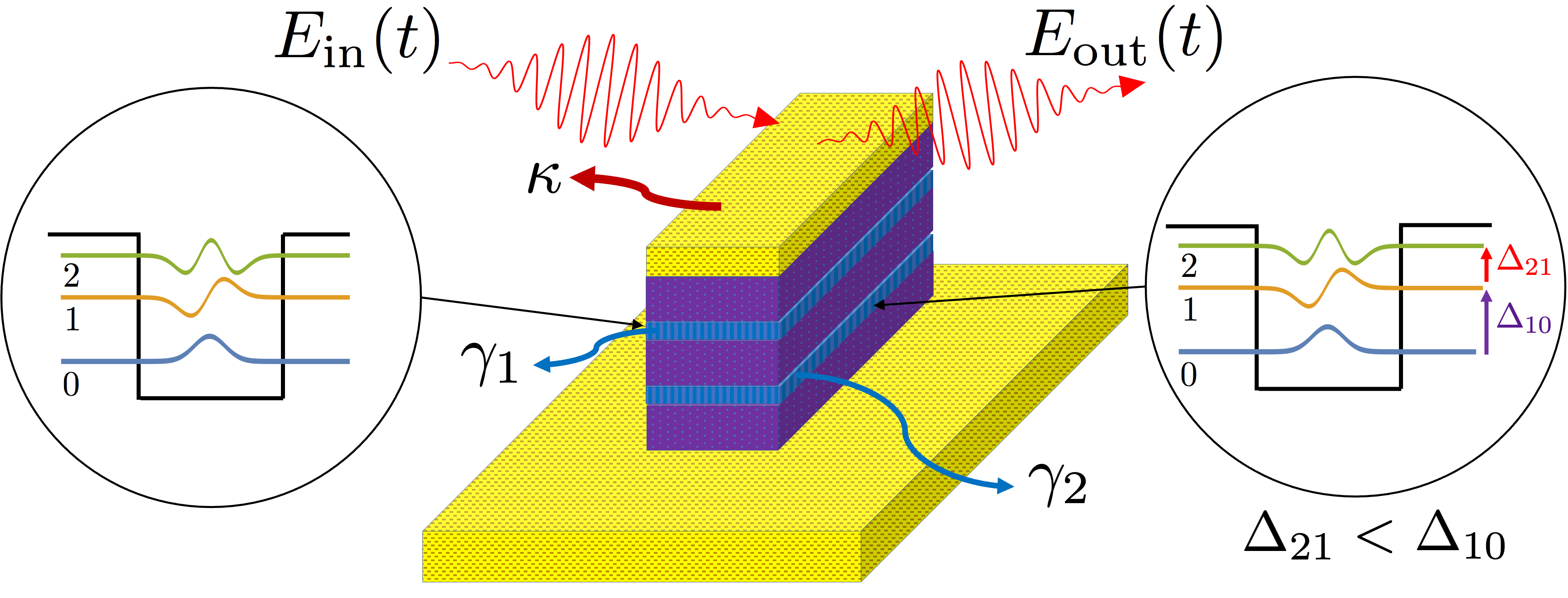
Figure 1: Schematic picture of a MQW in a driven open infrared nanocavity. Two quantum wells forming a MQW with fundamental frequency $\omega_{0}=\Delta_{10}$. The $0\to 1$ and $1\to 2$ transitions are coupled to the near-field of an open nanocavity with frequency $\omega_{\mathrm{c}}$ by an incoming laser pulse $E_{\mathrm{in}}$. The photons that leak out the nanocavity on sub-picosecond time scales at rate $\kappa$ generate the free-induction decay (FID) signal encoded in the outcoming field $E_{\mathrm{out}}$.

We consider a small number $N$ of quantum wells located within the near field of a resonant infrared nanoantenna, as illustrated in Fig. 1. The quantum wells do not interact with each other and have discrete intersubband energy levels with transition frequencies in the THz regime Miller (1997). The bare Hamiltonian of the MQW system is a collection of anharmonic quantum Kerr oscillators ( $\hbar\equiv 1$ throughout)

$$\hat{H}_{n}=\omega_{n}\hat{b}_{n}^{\dagger}\hat{b}_{n}-U_{n}\hat{b}_{n}^{\dagger}\hat{b}_{n}^{\dagger}\hat{b}_{n}\hat{b}_{n},$$ (1)

where $\hat{b}_{n}$ is the annihilation operator of the $n$-th quantum well dipole, $\omega_{n}$ is the fundamental frequency and $U_{n}$ the anharmonicity parameter. The geometry of the quantum well structure determines the confined charge carriers potential and the spectral anharmonicity Goulain et al. (2023).

Projecting into a complete eigenbasis $|\nu_{n}\rangle$, Eq. (1) can be written as $\hat{H}_{n}=\sum_{\nu}E_{\nu_{n}}|\nu_{n}\rangle\langle\nu_{n}|$, with eigenvalues $E_{\nu_{n}}=\omega_{n}\nu_{n}-U_{n}(\nu_{n}^{2}-\nu_{n})$. The energy difference between consecutive levels of the $n$-th quantum well is $E_{\nu+1}-E_{\nu}=\omega_{n}-2U_{n}\nu$. The nonlinear parameter $U_{n}$ thus lowers the energy spacing of the $1\rightarrow 2$ excitation by $\Delta=2U_{n}$ relative to the fundamental frequency. In comparison with molecular vibrations, for which $\Delta\sim 10-40$ cm^-1 (Fulmer et al., 2004; Dunkelberger et al., 2019), multi-quantum well dipoles enable much larger anharmonicities, with $U_{n}\sim 100-300$ cm^-1 (Mann et al., 2021).

The anharmonic quantum wells couple to a common resonator near field $\hat{a}$, as described by the Hamiltonian

$$\hat{\mathcal{H}}=\omega_{\rm c}\hat{a}^{\dagger}\hat{a}+\sum_{n=1}^{N}\left[\hat{H}_{n}+g_{n}(\hat{a}\hat{b}^{\dagger}_{n}+\hat{a}^{\dagger}\hat{b}_{n})\right],$$ (2)

where $\omega_{\rm c}$ is the resonant field mode frequency and $g_{n}=\mathcal{E}_{0}d_{0}$ is the light-matter coupling strength. The latter depends on the square-root amplitude of the vacuum fluctuations $\mathcal{E}_{0}$ and the transition dipole moment $d_{0}$. For simplicity, we assume transition dipoles are state-independent but other choices do not qualitatively affect the results.

We calculate the dissipative dynamics of the system in the presence of a driving pulse according to the Lindblad quantum master equation

$$\frac{\rm d}{\rm dt}\hat{\rho}=-\dot{\imath}[\hat{\mathcal{H}}+\hat{H}_{\rm d}(t),\hat{\rho}]+\mathcal{L}_{\kappa}[\hat{\rho}]+\mathcal{L}_{\gamma}[\hat{\rho}].$$ (3)

where $\hat{\rho}$ is the density matrix of the total cavity-MQW system. $\mathcal{L}_{\kappa}[\hat{\rho}]$ and $\mathcal{L}_{\gamma}[\hat{\rho}]$ are photonic and material relaxation superoperators given by

$$\mathcal{L}_{\kappa}[\hat{\rho}] = \frac{\kappa}{2}\left(2\,\hat{a}\hat{\rho}\hat{a}^{\dagger}-\hat{a}^{\dagger}\hat{a}\,\hat{\rho}-\hat{\rho}\,\hat{a}^{\dagger}\hat{a}\right),$$ (4)

$$\mathcal{L}_{\gamma}[\hat{\rho}] = \sum_{n=1}^{N}\frac{\gamma_{n}}{2}\left(2\,\hat{b}_{n}\hat{\rho}\hat{b}_{n}^{\dagger}-\hat{b}_{n}^{\dagger}\hat{b}_{n}\,\hat{\rho}-\hat{\rho}\,\hat{b}_{n}^{\dagger}\hat{b}_{n}\right).$$ (5)

where $\kappa$ and $\gamma_{n}$ are the decay rates of photonic and $n$-th quantum well modes, respectively. The decoherence processes encoded in $\gamma_{n}$ are mainly given by the interaction between MQW and the thermalized phonon bath of the semiconductor structure (Levine, 1993). For the open cavity field, the main source of decoherence is non radiative decay in the metal (Mann et al., 2020), as well as radiative losses (Triana et al., 2022). The time-dependent Hamiltonian $\hat{H}_{\rm d}(t)$ that describes the driving pulse is given by

$$\hat{H}_{\rm d}(t)=F_{0}\varphi(t)(\hat{a}e^{i\omega_{\rm d}t}+\hat{a}^{\dagger}e^{-i\omega_{\rm d}t}),$$ (6)

with the Gaussian pulse envelope $\varphi(t)=\exp[-(t-t_{0})^{2}/(2T^{2})]$ and carrier frequency $\omega_{\rm d}$. $|F_{0}|^{2}$ is proportional to the incoming photon flux , $t_{0}$ is the pulse center time and and $T$ is the pulse duration.

III Mean-field Nonlinear chirping model

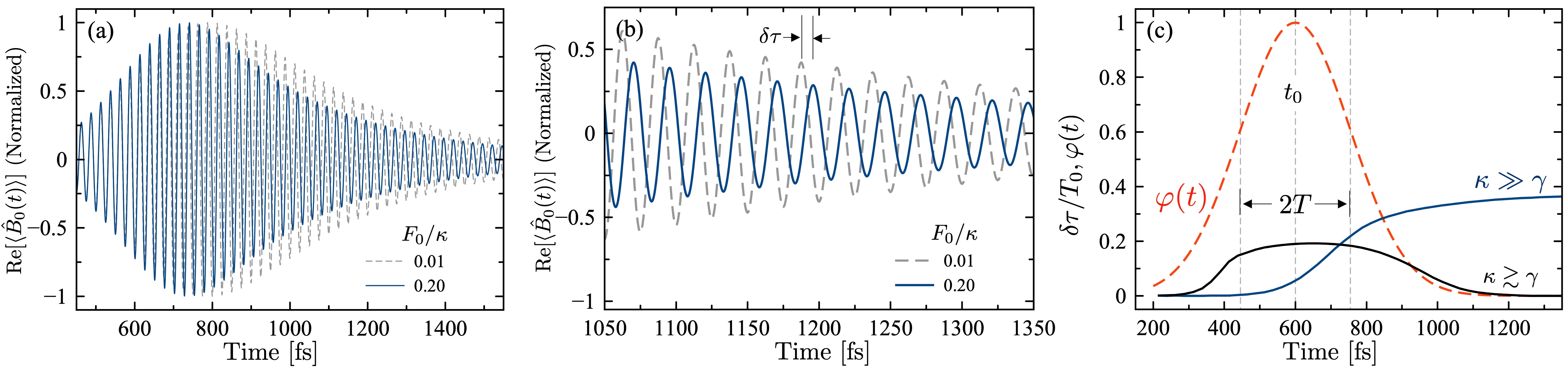
Figure 2: Dipolar FID signals. (a) Real part of the material collective coherence $\text{Re}\langle\hat{B}_{0}(t)\rangle$ for two identical quantum wells coupled to a common field mode. The antenna is driven by a laser pulse with a carrier frequency $\omega_{\rm d}$, pulse duration $T=155$ fs and centered at $t_{0}=600$ fs for laser intensities $F_{0}=0.01\kappa$ and $F_{0}=0.20\kappa$. Additional parameters are $\{\omega_{0},\kappa,\gamma,U,\sqrt{N}g\}=\{40.0,12.0,0.6,0.6,1.0\}$ THz. (b) Zoom of a fraction of the FID signals shown in (a) to visualize the time delay $\delta\tau$ generated in $t>t_{0}+2T$. (c) Time delay ratio calculated as the time difference between peaks and dips of the material collective coherence for $\gamma=0.6\text{ THz}$ (blue curve, different material and nanocavity bandwidths) and $\gamma=10.0\text{ THz}$ (black curve, comparable bandwidths). Dashed red line corresponds to the Gaussian pulse envelope.

We assume that the system dynamics involves only the lowest three energy levels of the quantum wells (i.e. $\nu_{\rm max}=2$). To ensure that higher energy levels do not participate in the evolution, we assume weak driving conditions, $F_{0}/\kappa<1$. Mean-field equations of motion for identical quantum wells can be obtained from Eq. (3) for light and matter coherences, to give coupled non-linear system

$$\frac{\rm d}{\rm dt}\left\langle\hat{a}\right\rangle =-\left(\frac{\kappa}{2}+i\omega_{\rm c}\right)\left\langle\hat{a}\right\rangle-i\sqrt{N}g\langle\hat{B}_{0}\rangle-i\tilde{F}_{\rm d}(t)$$ (7)

$$\frac{\rm d}{\rm dt}\langle\hat{B}_{0}\rangle =-\left[\frac{\gamma}{2}+i\left(\omega_{0}-\frac{2U}{N}|\langle\hat{B}_{0}\rangle|^{2}\right)\right]\langle\hat{B}_{0}\rangle-i\sqrt{N}g\langle\hat{a}\rangle,$$ (8)

where $\hat{B}_{0}=(1/\sqrt{N})\sum_{n}\hat{b}_{n}$ is the bright collective oscillator mode of fundamental frequency $\omega_{0}$ and decay rate $\gamma$. The driving parameter is $\tilde{F}_{\mathrm{d}}=F_{0}\varphi(t)\exp(-i\omega_{\mathrm{d}}t)$. For simplicity we set $g_{n}=g$ and $U_{n}=U$. For homogeneous systems, the $N-1$ dark collective modes $\hat{B}_{\alpha}=(1/\sqrt{N})\sum_{n}c_{\alpha,n}\hat{b}_{n}$, with $c_{\alpha,n}=\exp(i2\alpha n/N)$, evolve completely decoupled from Eqs. (7) and (8) (see Appendix A). The Kerr nonlinearity generates an effective dipole chirping effect, with instantaneous frequency

$$\omega^{\prime}_{0}(t)=\omega_{0}-\frac{2U}{N}|\langle\hat{B}_{0}(t)\rangle|^{2}.$$ (9)

This is red shifted from the fundamental resonance by an amount proportional to the bright mode occupation. The nonlinearity is proportional to the anharmonicity parameter $U$ and is small for large $N$ Triana et al. (2022). The transient red shift occurs while the system is driven by the laser pulse, which populates $\hat{B}_{0}(t)$, and is thus proportional to the photon flux parameter $F_{0}$.

We solve Eqs. (7) and (8) analytically to gain insight on the chirping effect. We assume that the bandwidth of the dipole resonance is much smaller than the antenna bandwidth, i.e., $\kappa\gg\gamma$. By adiabaticaly eliminating the antenna field from the dynamics, the evolution of bright mode after the pulse is over is given by

$$\langle\hat{B}_{0}(t)\rangle =B_{\rm off}e^{-\frac{\tilde{\gamma}}{2}(t-t_{\rm off})}e^{i\phi(t)}$$ (10)

where $t_{\mathrm{off}}$ is the pulse turn-off time. The phase evolves as

$$\phi(t) =\phi_{\rm off}+\frac{2UB_{\rm off}^{2}}{N\tilde{\gamma}}\left\{1-e^{-\tilde{\gamma}(t-t_{\rm off})}\right\},$$ (11)

where $\tilde{\gamma}=\gamma(1+4Ng^{2}/\kappa\gamma)$ is the Purcell-enhanced dipole decay rate Plankensteiner et al. (2019); Metzger et al. (2019) and $B_{\rm off}=|\langle\hat{B}_{0}(t_{\rm off})\rangle|$. Defining $\tau=t-t_{\rm off}$, in the long time regime, $\tau\tilde{\gamma}\gg 1$, Eq. (11) gives the stationary relative phase

$$\Delta\phi_{\rm ss}=\phi_{\rm ss}-\phi_{\rm off}=\frac{2UB_{\rm off}^{2}}{N\tilde{\gamma}},$$ (12)

which depends quadratically on the laser strength, through the implicit linear dependence of $B_{\rm off}$ on $F_{0}$. The derivation of Eq. (11) can be found in Appendix B. In the limiting cases of harmonic oscillators ($U=0$), thermodynamic limit ($N\to\infty$), or linear response ($F_{0}/\kappa\ll 1$), the relative phase is neglegible $(\Delta\phi_{\mathrm{ss}}\approx 0)$. Molecular ensembles have low anharmonicites, and have been shown to require higher pulse strengths to produce finite relative phases Triana et al. (2022) than the ones discussed here.

Figures 2a and 2b show the evolution of the dipole coherence $\mathrm{Re}[\langle\hat{B}_{0}(t)\rangle]$ obtained by solving Eqs. (7)-(8) numerically with parameters relevant for experimental implementations Mann et al. (2021); Goulain et al. (2023). Figure 2b shows the time delay $\delta\tau$ produced by a strong driving pulse ($F_{0}/\kappa=0.2$) on the FID signal, in comparison with weak pulses. The delay $\delta\tau$ in time domain results in the relative phase from Eq. (12). Recent experiments with infrared nanoantennas have the femtosecond temporal resolution necessary to measure $\delta\tau$ Metzger et al. (2019); Triana et al. (2022).

Figure 2c shows the evolution of $\delta\tau$ for two scenarios. For long dipole lifetimes ($\gamma\ll\kappa$), i.e., narrowband MQW response, the time delay of the FID signal remains after the driving pulse is over. On the contrary, when $\gamma\sim\kappa$ the time delay disappears after the pulse ends. The system thus requires long dipole dephasing times to imprint a stationary time delay in the near field once the driving pulse is turned off.

IV Nonlinear phase shift in the frequency domain

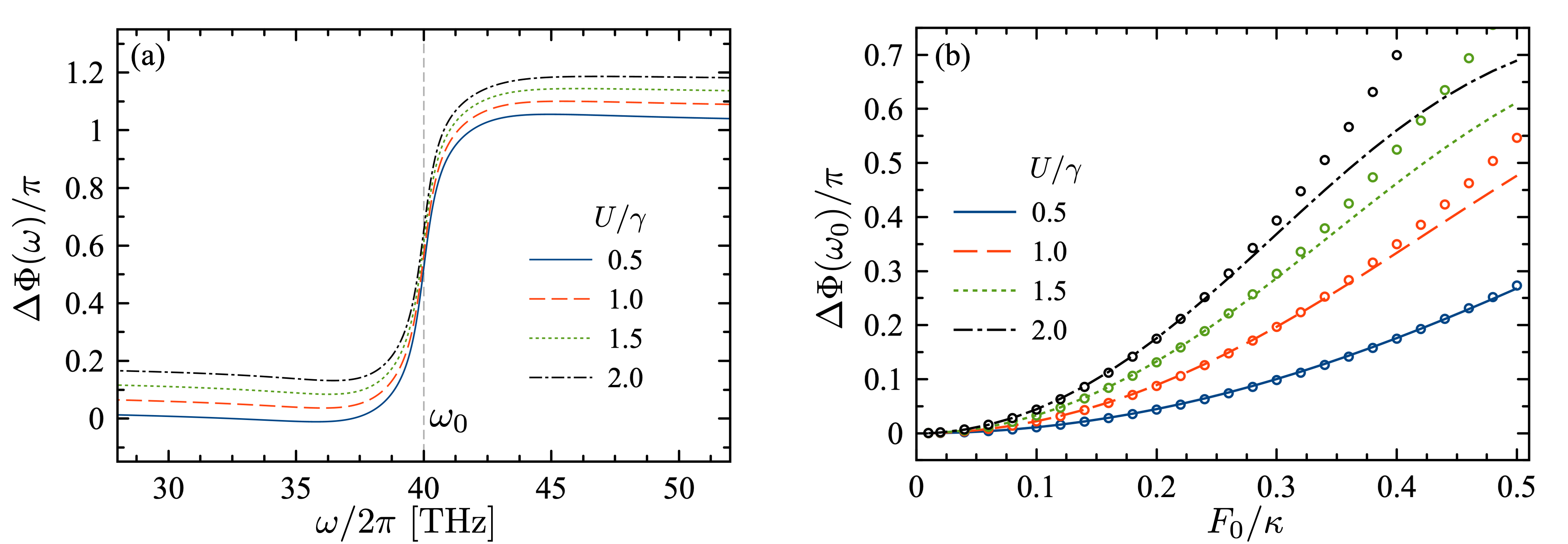
Figure 3: Intensity-dependent phase spectrum of the scattered field. (a) Relative phase spectrum $\Delta\Phi(\omega)$ for $F_{0}=0.2\kappa$ and different values of $U/\gamma$. (b) Nonlinear phase spectrum $\Delta\Phi(\omega_{0})/\pi$ at $\omega_{0}$ as a function of laser strength parameter $F_{0}/\kappa$. Circles correspond to analytical quadratic fitting with fit parameter $\alpha=3.5$ for all $U/\gamma$ cases . Both panels are calculated using Eq. (14) for different ratios $U/\gamma$. Additional parameters are $\{\omega_{0},\kappa,\gamma,\sqrt{N}g\}=\{40.0,12.0,0.6,1.0\}$ THz.

The time delay in the collective material coherence $\langle\hat{B}_{0}(t)\rangle$ from Fig. 2 is transferred to the photonic coherence $\langle\hat{a}(t)\rangle$, which ultimately gives the observable FID signal in heterodyne measurements Triana et al. (2022); Metzger et al. (2019). We define the Fourier transform of the field coherence as

$$\langle\hat{a}(\omega)\rangle=\frac{1}{\sqrt{2\pi}}\int_{-\infty}^{\infty}{\rm d}t\langle\hat{a}(t)\rangle e^{i\omega t},$$ (13)

and calculate the phase response $\Phi(\omega)$ of the FID signal as

$$\Phi(\omega)=\arctan\left(\frac{\text{Im}[\langle\hat{a}(\omega)\rangle]}{\text{Re}[\langle\hat{a}(\omega)\rangle]}\right).$$ (14)

The Fourier transform is taken for the post-pulse FID signal. Fig. 3a shows the phase spectrum for different values of the parameter $U/\gamma$, at fixed driving strength $(F_{0}=0.2\kappa)$. The relative phase in Fourier space is negligible for the limiting cases discussed above. In the case of anharmonic MQWs, the relative phase $\Delta\Phi(\omega)=\Phi(\omega)-\Phi_{\rm harm}$ increases as the anharmonicity parameter $U/\gamma$ grows for fixed $F_{0}$, with $\Phi_{\rm harm}$ given by relative phase obtained under harmonic conditions.

To gain insight on the behavior of the relative nonlinear phase, we use Eq. (10) to calculate $\Delta\Phi(\omega)$ analytically in the Fourier domain. We obtain

$$\Delta\Phi(\omega_{0})=\alpha\frac{2U}{N\tilde{\gamma}}\left(\frac{F_{0}}{\kappa}\right)^{2},$$ (15)

where the numerical parameter $\alpha$ comes from the proportionality relation $|\langle\hat{B}_{0}(t)\rangle|\propto F_{0}$ and the fact that $\phi_{\rm off}$ in Eq. (11) is also a nonlinear phase that grows with the dipole amplitude before the driving pulse is off. The derivation of Eq. (15) and additional details can be found in Appendix B. Figure 3b shows the analytical fitting and numerical calculations for the nonlinear phase shift at the fundamental frequency $\omega_{0}$ as a function of the laser intensity parameter $F_{0}/\kappa$, for different values of $U/\gamma$. In the low anharmonicity regime $U/\gamma<1$, the nonlinear phase has a clear quadratic dependence on $F_{0}$, while for strong anharmonicities $U/\gamma\gtrsim 1$, $\Delta\Phi(\omega_{0})$ is quadratic for only up to a certain driving strength. Beyond this point, higher energy levels ($\nu>2$) start to contribute with the dynamics of the system and the adiabatic elimination approach used to derive Eq. (15) breaks down.

V Nonlinear phase shift enhancement via dark states

The dynamics in the totally symmetric case with identical QW dipoles only involves the field and bright collective modes without the influence of the dark manifold. For a pair of inhomogeneous QWs ($N=2$), the equation of motion for the bright mode $\langle\hat{B}_{0}\rangle$ should be extended to read

$$\frac{\rm d}{\rm dt}\langle\hat{B}_{0}\rangle =-\left(\frac{\bar{\gamma}}{2}+i\bar{\omega}(t)\right)\langle\hat{B}_{0}\rangle-\left(\frac{\Delta\gamma}{2}+i\Delta\omega(t)\right)\langle\hat{B}_{1}\rangle$$

$$\quad-i\sqrt{N}g\langle\hat{a}\rangle$$ (16)

where $\langle\hat{B}_{1}\rangle=(-\langle\hat{b}_{1}\rangle+\langle\hat{b}_{2}\rangle)/\sqrt{2}$ is the dark mode for the pair of dipoles, $\bar{\gamma}=(\gamma_{1}+\gamma_{2})/2$ and $\Delta\gamma=(\gamma_{2}-\gamma_{1})/2$ are the average value and the mismatch of decay rates, respectively. The instantaneous average frequency is now given by

$$\bar{\omega}(t) =\bar{\omega}-U\left(|\langle\hat{B}_{0}(t)\rangle|^{2}+|\langle\hat{B}_{1}(t)\rangle|^{2}\right)$$ (17)

and the frequency mismatch by

$$\Delta\omega(t) =\Delta\omega-2U{\rm Re}\left[\langle\hat{B}_{0}(t)\rangle^{*}\langle\hat{B}_{1}(t)\rangle\right],$$ (18)

where $\bar{\omega}=(\omega_{1}+\omega_{2})/2$ and $\Delta\omega=(\omega_{2}-\omega_{1})/2$. The coupling of the dark mode $\langle\hat{B}_{1}\rangle$ with the bright mode influences the dynamics of the system. It is clear that in the totally symmetric case ($\Delta\gamma=\Delta\omega=0$), bright and dark modes are decoupled and Eq. (V) reduces to Eq. (8). The positive additive contribution $|\langle\hat{B}_{1}\rangle|^{2}$ to the instantaneous dipole frequency suggests that the dark manifold enhances the nonlinear phase shift. The derivation of Eq. (V) can be found in Appendix C.

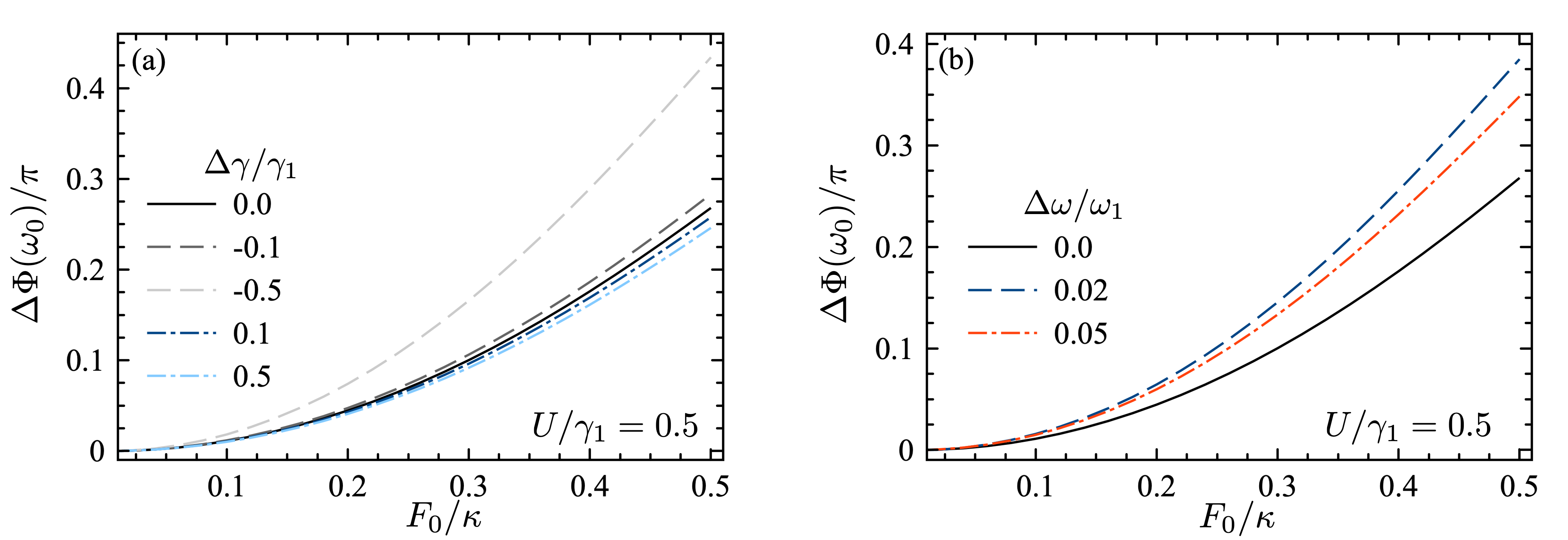
Figure 4: Nonlinear phase shift enhancement via dipole inhomogeneity. Nonlinear phase shift at $\omega_{0}$ as a function of the driving ratio $F_{0}/\kappa$ for the anharmonicity parameter $U/\gamma=0.5$. (a) For $\omega_{1}=\omega_{2}=\omega_{0}$ and $\gamma_{1}\neq\gamma_{2}$. (b) For $\omega_{0}=\omega_{1}\neq\omega_{2}$ and $\gamma_{1}=\gamma_{2}$. Additional parameters are $\{\omega_{0},\kappa,\gamma_{1},\sqrt{N}g\}=\{40.0,12.0,0.6,1.0\}$ THz.

Figure 4 shows the nonlinear phase spectrum of $\langle\hat{a}(\omega)\rangle$ evaluated at the fundamental frequency $\omega_{0}$ for two inhomogeneus scenarios. First, we set equal fundamental frequencies with variations in the decay rates of the QWs, i.e., $\omega_{1}=\omega_{2}=\omega_{0}$ and $\gamma_{1}\neq\gamma_{2}$. In Fig. 4a we find both enhancement and reduction of the nonlinear phase for $U=0.5\gamma_{1}$. Enhancement is reached for $\Delta\gamma<0$, which is due to a reduction of the effective decay rate $\bar{\gamma}$ associated with bright mode in Eq. (V). In the opposite case, i.e., for $\gamma_{2}>\gamma_{1}$, $\Delta\Phi(\omega_{0})$ decreases due to the increased decay rate of the bright mode. The second scenario considers one QW detuned with respect to the other but both having equal decay rates, i.e., $\omega_{1}\neq\omega_{2}$ and $\gamma_{1}=\gamma_{2}$. The results are shown in Fig. 4b. In this case, the small blue and red detuning of one of the quantum wells gives a nonlinear phase enhancement. However, for very large detunings ($\Delta\omega/\omega_{0}>0.1$) the nonlinear phase tends to the homogeneous limit ($\Delta\omega=0$), as the detuned quantum well becomes effectively decoupled from the field.

VI Validity of the mean-field theory

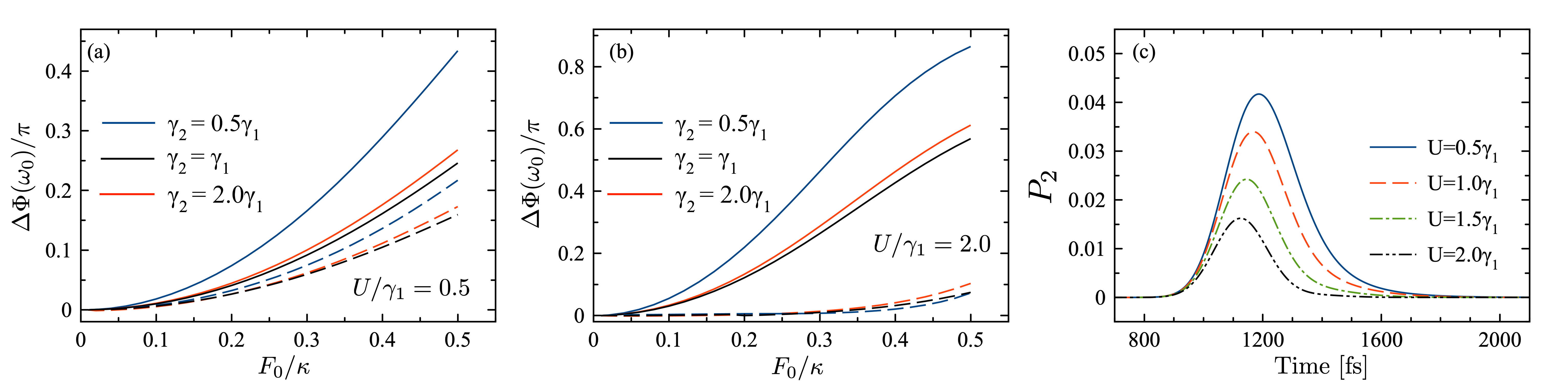
Figure 5: Fully quantum validation of the nonlinear phase shift. Relative nonlinear phase shift as a function of laser strength parameter $F_{0}/\kappa$ found in the mean-field approximation (solid lines) and by solving the Lindblad quantum master equation (dashed lines) for different inhomogeneous scenarios and for (a) $U/\gamma_{1}=0.5$ and (b) $U/\gamma_{1}=2.0$. (c) Population dynamics of the second excited energy level $P_{2}$ for $F_{0}=0.3\kappa$ and different values of the anharmonicity parameter $U/\gamma_{1}$. Additional parameters for all panels are $\{\omega_{0},\kappa,\gamma_{1},\sqrt{N}g\}=\{40.0,12.0,0.6,1.0\}$ THz.

We calculate the evolution of the total density matrix by solving the Lindblad quantum master equation in Eq. (3) to explore the regime of validity of the analytical theory for a pair of quantum well dipoles.

Figures 5a and 5b show the nonlinear phase shift $\Delta\Phi(\omega_{0})$ as a function of the laser strength parameter $F_{0}/\kappa$ predicted by the Lindblad QME for two different values of the anharmonicity: $U=0.5\gamma_{1}$ and $U=2.0\gamma_{1}$. For $U=0.5\gamma_{1}$, both mean-field (solid lines) and fully quantum (dashed lines) calculations agree up to a factor of two approximately. However, $\Delta\Phi(\omega_{0})$ in the mean-field approach is overestimated for $U=2.0\gamma_{1}$, where the nonlinear phase is negligible up to $F_{0}/\kappa\approx 0.4$, then increases for higher laser intensities. The latter is due to the large detuning between cavity frequency $\omega_{\mathrm{c}}$ and $\Delta_{21}$. As a consequence, anharmonic blockade is observed for the intersubband state $\nu=2$ such that the higher level does not participate in the dynamics, causing the dipole to behave effectively as a harmonic oscillator. In Fig. 5c, we show the population of the $\nu=2$ level ($P_{2}$) for $F_{0}/\kappa=0.3$ and different values of the anharmonicity parameter $U/\gamma_{1}$. $P_{2}$ is suppressed as $U$ increases due to the blockade effect. The mean-field theory is accurate for weak pulses ($F_{0}/\kappa<0.1$) independent on the anharmonicity parameter $U/\gamma$ and, for stronger pulses with anharmonicities lower than dissipation rate of MQWs ($U/\gamma<1.0$).

VII Discussion and Conclusion

In this work, we described a novel dynamical photon blockade mechanism in THz cavity QED that can be used for imprinting power-dependent phase shifts on the electromagnetic response of a coupled cavity-dipole system. We develop analytical quantum mechanical theory to model free-induction decay signals of a pulse-driven cavity system, using parameters that are relevant for quantum well intersubband transitions in mid-infrared resonators Mann et al. (2021). For $N$ quantum wells within the near field of the driven resonator, the theory shows that using only a moderately strong pulse that drives a small fraction of the intersubband level population to the second excitation manifold, a stationary phase shift proportional to the spectral anharmonicity parameter $U/N\gamma$ and the photon flux of the pulse, can be imprinted on the FID response of the near field, which can then be retrieved using time-domain spectroscopic techniques Wilcken et al. (2023). For experimentally relevant system parameters, nonlinear phase shifts of order of $1$ radian are predicted for a single quantum well using a single sub-picosecond pulse of few $\mu$W power.

The predicted phase nonlinearity can be physically understood as a result of laser-induced dipole effect that dynamically detunes the cavity field with respect to the $1\to 2$ intersubband transition, caused by population driven between the first and second excited levels of the anharmonic quantum well spectrum. The analytical model is validated numerically using density matrix solutions of the corresponding Lindblad quantum master equation. Notably, the proposed dipole chirping mechanism only occurs for cavity fields that are much shorter lived than the THz dipole resonance (bad cavity limit), as is the case in several nanophotonic setups Metzger et al. (2019); Mann et al. (2021). Moreover, the phase imprinting scheme works best in the weak coupling regime, contrary to conventional photon blockade effects developed for optical cavities QED, which require strong coupling conditions Birnbaum et al. (2005); Benea-Chelmus et al. (2019).

Our work demonstrates the feasibility of implementing nonlinear phase operations at THz frequencies using current available nanocavities Mann et al. (2021); Metzger et al. (2019); Wilcken et al. (2023) and contributes to the development of quantum optics in the high-THz regime Goulain et al. (2023); Benea-Chelmus et al. (2019), which can enable fundamental studies of cavity quantum electrodynamics De Liberato (2019); Wang and De Liberato (2021), material and molecular spectroscopy Kizmann et al. (2022); Wilcken et al. (2023); Bylinkin et al. (2021), and controlled chemistry in confined electromagnetic environments Nagarajan et al. (2021); Ahn et al. (2023). Extensions of this work to the analysis of THz and infrared pulses with non-classical field statistics Waks et al. (2004); Zhu et al. (2022) could open further possibilities for developing ultrafast quantum information processing at room temperature.

VIII Acknowledgments

M.A. is funded by ANID - Agencia Nacional de Investigación y Desarrollo through the Scholarship Programa Doctorado Becas Chile/2018 No. 21181591. J.F.T. is supported by ANID - Fondecyt Iniciación Grant No. 11230679. F.H. is funded by ANID - Fondecyt Regular Grant No. 1221420 and the Air Force Office of Scientific Research under award number FA9550-22-1-0245. A.D. is supported by ANID - Fondecyt Regular 1180558, Fondecyt Grants No. 1231940 and No. 1230586. All authors also thanks support by ANID - Millennium Science Initiative Program ICN17_012.

Appendix A MEAN-FIELD APPROACH FOR $N$ IDENTICAL DIPOLES

The density matrix of the light-matter system $\hat{\rho}(t)$ evolves according to the quantum master equation in Lindblad form

$$\frac{\rm d}{\rm dt}\hat{\rho}=-i[\hat{\mathcal{H}}+\hat{H}_{\rm d}(t),\hat{\rho}]+\mathcal{L}_{\kappa}\left[\hat{\rho}\right]+\mathcal{L}_{\gamma}\left[\hat{\rho}\right],$$ (19)

where $\hat{\mathcal{H}}$ is the Hamiltonian of the system in Eq. (2), $\hat{H}_{\mathrm{d}}$ is the time-dependent Hamiltonian of the laser pulse that drives the nanocavity in Eq. (6) and the Lindblad superoperators are given by Shammah et al. (2017); Manzano (2020)

$$\mathcal{L}_{\kappa}[\hat{\rho}] = \frac{\kappa}{2}\left(2\,\hat{a}\hat{\rho}\hat{a}^{\dagger}-\hat{a}^{\dagger}\hat{a}\,\hat{\rho}-\hat{\rho}\,\hat{a}^{\dagger}\hat{a}\right),$$ (20)

$$\mathcal{L}_{\gamma}[\hat{\rho}] = \sum_{n=1}^{N}\frac{\gamma_{n}}{2}\left(2\,\hat{b}_{n}\hat{\rho}\hat{b}_{n}^{\dagger}-\hat{b}_{n}^{\dagger}\hat{b}_{n}\,\hat{\rho}-\hat{\rho}\,\hat{b}_{n}^{\dagger}\hat{b}_{n}\right).$$ (21)

$\kappa$ is the resonator field decay rate and $\gamma_{n}$ is the MQW relaxation rate into a local reservoir. $\hat{a}$ and $\hat{b}_{n}$ are the annihilation operators of the field mode and the $n$-th quantum well, respectively.

The local operators can be expressed as a linear combination of the collective modes $\hat{B}_{\alpha}$ as

$$\hat{b}_{n}=\frac{1}{\sqrt{N}}\sum_{\alpha=0}^{N-1}\exp\left(-\frac{\dot{\imath}2\pi\alpha n}{N}\right)\hat{B}_{\alpha}.$$ (22)

Thus, the Lindblad superoperators for the collective modes considering homogeneous MQWs (with $\gamma_{n}=\gamma$) are given by

$$\mathcal{L}_{\gamma}[\hat{\rho}]=\frac{\gamma}{2}\sum_{\alpha=0}^{N-1}\left(2\,\hat{B}_{\alpha}\hat{\rho}\hat{B}_{\alpha}^{\dagger}-\{\hat{B}_{\alpha}^{\dagger}\hat{B}_{\alpha}\,,\hat{\rho}\}\right),$$ (23)

where $\{\hat{A},\hat{B}\}$ is the anticommutator between arbitrary operators $\hat{A}$ and $\hat{B}$.

The exact equations of motion for the field and bright collective matter coherences in the Schrödinger picture are given by

$$\frac{\rm d}{\rm dt}\left\langle\hat{a}\right\rangle =-\left(\frac{\kappa}{2}+i\omega_{\mathrm{c}}\right)\left\langle\hat{a}\right\rangle-i\sqrt{N}g\langle\hat{B}_{0}\rangle-i\tilde{F}_{\rm d}(t),$$ (24)

$$\frac{\rm d}{{\rm d}t}\langle{\hat{B}_{0}}\rangle =-\left({\gamma}/{2}+i\omega_{0}\right)\langle{\hat{B}_{0}}\rangle-i\sqrt{N}g\langle{\hat{a}}\rangle$$

$$\quad+i\frac{2U}{\sqrt{N}}\sum_{n=1}^{N}\langle{\hat{b}^{\dagger}_{n}\hat{b}_{n}\hat{b}_{n}}\rangle,$$ (25)

with $\tilde{F}_{\rm d}(t)=F_{0}\varphi(t)e^{-\dot{\imath}\omega_{\rm d}t}$. We calculate the collective matter coherence via $\langle\hat{B}_{0}\rangle=\sum_{n}{\rm Tr}[\hat{b}_{n}\hat{\rho}(t)]/\sqrt{N}$. Using Eq. (22), the third order term in Eq. (25) is given by an expansion of bright and dark collective operators as

$$\sum_{n}\hat{b}_{n}^{\dagger}\hat{b}_{n}\hat{b}_{n} =\frac{1}{N^{\frac{3}{2}}}\sum_{\beta,\eta,\epsilon=0}^{N-1}\left(\sum_{n}e^{\frac{\dot{\imath}2\pi}{N}(\beta-\eta-\epsilon)n}\right)\hat{B}_{\beta}^{\dagger}\hat{B}_{\eta}\hat{B}_{\epsilon},$$

$$=\frac{1}{\sqrt{N}}\sum_{\beta,\eta,\epsilon}(\delta_{\beta-\eta-\epsilon,0}+\delta_{\beta-\eta-\epsilon,-N})\hat{B}_{\beta}^{\dagger}\hat{B}_{\eta}\hat{B}_{\epsilon},$$

$$=\frac{1}{\sqrt{N}}(\hat{B}_{0}^{\dagger}\hat{B}_{0}\hat{B}_{0}+\hat{B}_{0}^{\dagger}\hat{B}_{1}\hat{B}_{1}+\ldots)$$ (26)

Taking the expectation value, the collective third order terms in Eq. (A) can be expressed as

$$\langle\hat{B}_{\beta}^{\dagger}\hat{B}_{\eta}\hat{B}_{\epsilon}\rangle\approx\langle\hat{B}_{\beta}\rangle^{*}\langle\hat{B}_{\eta}\rangle\langle\hat{B}_{\epsilon}\rangle.$$ (27)

The expansion has just one third order term with equal indexes and it is constrained to the bright mode operator ($\beta=\eta=\epsilon=0$), which implies that the remaining terms have at least one dark mode operator, i.e., a nonzero index. We consider that the laser pulse drives only the nanocavity, which just interacts with the bright mode [see Eq. (24)]. Hence, considering initial population of the dark modes equal to zero, the dark manifold is completely decoupled from the field $\langle\hat{a}\rangle$ and bright collective mode $\langle\hat{B}_{0}\rangle$. The latter is due to the only term in the expansion [Eq. (A)] that evolves to nonzero values is $|\langle\hat{B}_{0}\rangle|^{2}\langle\hat{B}_{0}\rangle$. As a consequence, the evolution of $\langle\hat{B}_{0}(t)\rangle$ reduces to Eq. (8).

Appendix B ADIABATIC ELIMINATION OF THE ANTENNA DYNAMICS

In the bad cavity limit, we can adiabatically eliminate the dynamics of the single field mode (${\rm d}\left\langle\hat{a}(t)\right\rangle/{\rm dt}\rightarrow 0$) since $\kappa\gg\gamma$ and $(\kappa-\gamma)/4>\sqrt{N}g$. We reduce the equations of motion to a single equation for bright collective matter coherence $\hat{B}_{0}$ which contains the influence of the open cavity mode. Hence, Eq. (24) in the rotating frame of the cavity frequency $\omega_{0}$ reduces to

$$\left\langle\tilde{a}^{\rm ad}(t)\right\rangle\approx-i\frac{2\sqrt{N}g}{\kappa}\langle\tilde{B}^{\rm ad}_{0}(t)\rangle-i\frac{2}{\kappa}F_{\rm d}(t),$$ (28)

and solving for $\langle\hat{B}_{0}\rangle$

$$\frac{\rm d}{\rm dt}\langle\tilde{B}^{\rm ad}_{0}(t)\rangle =-\frac{\tilde{\gamma}}{2}\langle\tilde{B}^{\rm ad}_{0}(t)\rangle-\frac{2\sqrt{N}g}{\kappa}F_{\rm d}(t)$$

$$\quad+i\frac{2U}{N}|\langle\tilde{B}^{\rm ad}_{0}(t)\rangle|^{2}\langle\tilde{B}^{\rm ad}_{0}(t)\rangle,$$ (29)

with the renormalized decay rate of the dipole coherence $\tilde{\gamma}=\gamma(1+4Ng^{2}/\kappa\gamma)$, which is commonly known as the Purcell factor Triana et al. (2022).

Equation (29) with $F_{\mathrm{d}}(t)=0$ is known in non-linear hydrodynamics as the Stuart-Landau oscillator equation Stuart (1958); Panteley et al. (2015). The laser pulse at a given time $t=t_{\mathrm{off}}$ turns off and Eq. (29) can be solved analytically by a slow variation of the dipole coherence in polar form as $\langle\tilde{B}^{\rm ad}_{0}(t)\rangle=|\langle\tilde{B}^{\rm ad}_{0}(t)\rangle|e^{i\phi(t)}$. Thus, the equations of motion for the amplitude and phase can be written as

$$\frac{\rm d}{\rm dt}|\langle\tilde{B}^{\rm ad}_{0}(t)\rangle| =-\frac{\tilde{\gamma}}{2}|\langle\tilde{B}^{\rm ad}_{0}(t)\rangle|$$ (30)

$$\frac{\rm d}{\rm dt}\phi(t) =2\frac{U}{N}|\langle\tilde{B}^{\rm ad}_{0}(t)\rangle|^{2}.$$ (31)

where their corresponding solutions are given by

$$|\langle\tilde{B}_{0}^{\rm ad}(t)\rangle| =B_{\rm off}e^{-\frac{\tilde{\gamma}}{2}(t-t_{\rm off})}$$ (32)

$$\phi(t) =\phi_{\rm off}+\frac{2UB_{\rm off}^{2}}{N\tilde{\gamma}}\left\{1-e^{-\tilde{\gamma}(t-t_{\rm off})}\right\}.$$ (33)

with $B_{\rm off}=|\langle\tilde{B}_{0}^{\rm ad}(t_{\rm off})\rangle|$ and $\phi_{\rm off}=\phi(t_{\rm off})$. The dipole coherence in the rotating frame of the laser evolves as

$$\langle\hat{B}_{0}^{\rm ad}(t)\rangle =\langle\hat{B}_{0}^{\rm ad}(t_{\rm off})\rangle e^{-\frac{\tilde{\gamma}}{2}(t-t_{\rm off})}e^{-i\omega_{0}(t-t_{\rm off})}$$

$$\quad\times\exp[i\Delta\phi_{\rm ss}(1-\exp[-\tilde{\gamma}(t-t_{\rm off})])],$$ (34)

where $\Delta\phi_{\rm ss}=\phi_{\rm ss}-\phi_{\rm off}$ and $\langle\hat{B}_{0}^{\rm ad}(t_{\rm off})\rangle=B_{\rm off}e^{i\phi_{\rm off}}$. The exponential that depends on the relative phase $\Delta\phi$ in Eq. (B) evidences the nonlinear contributions, instead of the solution with harmonic MQWs or in the weak driving regime. To clarify, the analogous solution of the dipole coherence with $U=0$ [$\hat{B}_{0,{\rm L}}^{\rm ad}(t)$] for $t\geq t_{\rm off}$ is given by

$$\langle\hat{B}_{0,{\rm L}}^{\rm ad}(t)\rangle=-\beta(T)\frac{2\sqrt{N}gF_{0}}{\kappa}e^{-(\tilde{\gamma}/2+i\omega_{0})t}$$ (35)

where the factor $\beta(T)$ depends on the envelope functional shape, and the stationary phase $\Delta\phi_{\rm ss}=0$ due to the system evolves with a constant phase $\phi_{\rm ss}=\phi_{\rm off}$.

In the case of the phase, Eq. (33) describes a stationary phase $\phi(t)=\phi_{\rm ss}$ in the long time regime ($t\gg t_{\mathrm{off}}$), which is given by

$$\phi_{\rm ss}=\phi_{\rm off}+\frac{2UB_{\rm off}^{2}}{N\tilde{\gamma}}.$$ (36)

Note that the expression is quadratic respect to amplitude $B_{\mathrm{off}}$ and constant for harmonic MQWs ($U=0$).

B.1 Relation between the dipole and cavity phase shifts

We measure the free-induction decay signal in the laboratory, which is related with the field mode coherence $\langle\hat{a}\rangle$. Here, we connect the phase shift that can be obtained from experiments with the phase from the dipole coherence. We define the relative nonlinear phase shift in frequency domain at $\omega_{0}$ in terms of the Fourier transform of the cavity coherence, $\langle\hat{a}(\omega)\rangle=\mathcal{F}[\langle\hat{a}(t)\rangle](\omega)$, as

$$\Delta\Phi(\omega_{0})=\Phi(\omega_{0})-\Phi_{\rm harm}(\omega_{0}),$$ (37)

where,

$$\Phi(\omega)=\arctan\left(\frac{{\rm Im}[\langle\hat{a}(\omega)\rangle]}{{\rm Re}[\langle\hat{a}(\omega)\rangle]}\right)$$ (38)

and $\Phi_{\rm harm}=\lim_{F_{0}/\kappa\ll 1}\Phi(\omega_{0})$. The latter is valid since the response of the anharmonic dipole oscillator under weak driving conditions $F_{0}/\kappa\ll 1$ or in the limit of negligible anharmonicity $U/\gamma\to 0$ is equivalent to the linear response, as it is shown in Eq. (36). Assuming the same $t_{\mathrm{off}}$ for the cavity and dipole coherences, the equations of motion for the field coherence and phase in frequency domain are given by

$$\langle\hat{a}(\omega)\rangle =-ig_{N}\langle\hat{B}_{0}(\omega)\rangle\frac{1}{\kappa/2-i(\omega-\omega_{\rm c})},$$ (39)

$$\Phi(\omega_{0}) =\Phi^{(0)}(\omega_{0})+\arctan\left(\frac{\omega_{0}-\omega_{\rm c}}{\kappa/2}\right)-\frac{\pi}{2},$$ (40)

with

$$\Phi^{(0)}(\omega_{0})=\arctan\left(\frac{{\rm Im}[\langle\hat{B}_{0}(\omega_{0})\rangle]}{{\rm Re}[\langle\hat{B}_{0}(\omega_{0})\rangle]}\right).$$

The second and third term in Eq. (40) are independent on anharmonicity parameter $U/\kappa$ and driving strength $F_{0}/\kappa$. Thus, in analogy with Eq. (37), i.e., considering that the relative phase shift is given in terms of the linear response and nonlinear contributions, we can write $\Delta\Phi(\omega_{0})$ as a function of the dipole coherence instead of the field mode response as

$$\Delta\Phi(\omega_{0})=\Delta\Phi^{(0)}(\omega_{0})=\Phi^{(0)}(\omega_{0})-\Phi_{\rm harm}^{(0)}(\omega_{0}),$$ (41)

where $\Phi_{\rm harm}^{(0)}(\omega_{0})=\lim_{F_{0}/\kappa\ll 1}\Phi^{(0)}(\omega_{0})$.

B.2 Nonlinear phase shift ansatz for an arbitrary driving pulse

We introduce an ansatz for the relative phase since the amplitude $|B_{\rm off}|$ cannot be defined for general driving pulses. We define the nonlinear phase shift $\Delta\Phi$ at frequency $\omega_{0}$ as

$$\Delta\Phi(\omega_{0})=\alpha\frac{2U}{N\tilde{\gamma}}\left(\frac{F_{0}}{\kappa}\right)^{2},$$ (42)

where $\alpha$ is a phenomenological parameter to be explored. The definition in Eq. (42) is possible considering that the squared amplitude of the dipole coherence [Eq. (32)] and the stationary phase [Eq. (36)] grow proportional to the square of the driving strength for the ratio $F_{0}/\kappa<1$. Further, numerical results in Fig. 3 suggest the quadratic dependence.

Appendix C MEAN-FIELD CHIRPING MODEL FOR TWO ASYMMETRIC QUANTUM WELLS

From the local quantum master equation, the mean-field equations of motion for the coherences of the inhomogeneous quantum wells ($\hat{b}_{1}$ and $\hat{b}_{2}$) and field mode $\hat{a}$ are given by

$$\frac{\rm d}{\rm dt}\langle\hat{a}\rangle =-\left(\frac{\kappa}{2}+i\omega_{\rm c}\right)\langle\hat{a}\rangle-ig(\langle\hat{b}_{1}\rangle+\langle\hat{b}_{2}\rangle)-i\tilde{F}_{\rm d}(t),$$ (43)

$$\frac{\rm d}{\rm dt}\langle\hat{b}_{1}\rangle =-\left(\frac{\gamma_{1}}{2}+i\omega_{\rm 1}\right)\langle\hat{b}_{1}\rangle-ig\langle\hat{a}\rangle+i2U|\langle\hat{b}_{1}\rangle|^{2}\langle\hat{b}_{1}\rangle,$$ (44)

$$\frac{\rm d}{\rm dt}\langle\hat{b}_{2}\rangle =-\left(\frac{\gamma_{2}}{2}+i\omega_{\rm 2}\right)\langle\hat{b}_{2}\rangle-ig\langle\hat{a}\rangle+i2U|\langle\hat{b}_{2}\rangle|^{2}\langle\hat{b}_{2}\rangle.$$ (45)

We set equal light-matter coupling strengths $g=g_{1}=g_{2}$ and anharmonicity parameters $U=U_{1}=U_{2}$. By replacing the bright $\hat{B}_{0}=(\hat{b}_{1}+\hat{b}_{2})/\sqrt{2}$ and dark $\hat{B}_{1}=(-\hat{b}_{1}+\hat{b}_{2})/\sqrt{2}$ modes, we obtain

$$\frac{\rm d}{\rm dt}\langle\hat{a}\rangle =-\left(\frac{\kappa}{2}+i\omega_{\rm c}\right)\langle\hat{a}\rangle-ig\langle\hat{B}_{0}\rangle-i\tilde{F}_{\rm d}(t),$$ (46)

$$\begin{split}\frac{\rm d}{\rm dt}\langle\hat{B}_{0}\rangle&=-\left(\frac{\bar{\gamma}}{2}+i\bar{\omega}(t)\right)\langle\hat{B}_{0}\rangle-\left(\frac{\Delta\gamma}{2}+i\Delta\omega(t)\right)\langle\hat{B}_{1}\rangle\\ &\quad-ig\langle\hat{a}\rangle,\end{split}$$ (47)

$$\begin{split}\frac{\rm d}{\rm dt}\langle\hat{B}_{1}\rangle&=-\left(\frac{\bar{\gamma}}{2}+i\bar{\omega}(t)\right)\langle\hat{B}_{1}\rangle-\left(\frac{\Delta\gamma}{2}+i\Delta\omega(t)\right)\langle\hat{B}_{0}\rangle,\end{split}$$ (48)

with

$$\bar{\omega}(t) =\bar{\omega}-U\left(|\langle\hat{B}_{0}(t)\rangle|^{2}+|\langle\hat{B}_{1}(t)\rangle|^{2}\right),$$

and

$$\Delta\omega(t) =\Delta\omega-2U{\rm Re}[\langle\hat{B}_{0}(t)\rangle^{*}\langle\hat{B}_{1}(t)\rangle].$$

where $\bar{\zeta}=(\zeta_{1}+\zeta_{2})/2$ and $\Delta\zeta=(\zeta_{2}-\zeta_{1})/2$, with $\zeta=\{\gamma,\omega\}$, are the average and mismatch values.

References

- Haroche et al. (2020) S. Haroche, M. Brune, and J. M. Raimond, Nature Physics 16, 243 (2020).
- O’Brien et al. (2009) J. L. O’Brien, A. Furusawa, and J. Vučković, Nature Photonics 3, 687 (2009).
- Kimble (1998) H. J. Kimble, Physica Scripta 1998, 127 (1998).
- Ruddell et al. (2017) S. K. Ruddell, K. E. Webb, I. Herrera, A. S. Parkins, and M. D. Hoogerland, Optica 4, 576 (2017).
- Mabuchi and Doherty (2002) H. Mabuchi and A. C. Doherty, Science 298, 1372 (2002).
- Vahala (2003) K. J. Vahala, Nature 424, 839 (2003).
- Ballarini and De Liberato (2019) D. Ballarini and S. De Liberato, Nanophotonics 8, 641 (2019).
- Kiraz et al. (2003) A. Kiraz, C. Reese, B. Gayral, L. Zhang, W. V. Schoenfeld, B. D. Gerardot, P. M. Petroff, E. L. Hu, and A. Imamoğlu, Journal of Optics B: Quantum and Semiclassical Optics 5, 129 (2003).
- Blais et al. (2004) A. Blais, R.-S. Huang, A. Wallraff, S. M. Girvin, and R. J. Schoelkopf, Phys. Rev. A 69, 062320 (2004).
- Fink et al. (2008) J. M. Fink, M. Göppl, M. Baur, R. Bianchetti, P. J. Leek, A. Blais, and A. Wallraff, Nature 454, 315 (2008).
- Putz et al. (2014) S. Putz, D. O. Krimer, R. Amsüss, A. Valookaran, T. Nöbauer, J. Schmiedmayer, S. Rotter, and J. Majer, Nature Physics 10, 720 (2014).
- Reagor et al. (2016) M. Reagor, W. Pfaff, C. Axline, R. W. Heeres, N. Ofek, K. Sliwa, E. Holland, C. Wang, J. Blumoff, K. Chou, M. J. Hatridge, L. Frunzio, M. H. Devoret, L. Jiang, and R. J. Schoelkopf, Phys. Rev. B 94, 014506 (2016).
- Blais et al. (2020) A. Blais, S. M. Girvin, and W. D. Oliver, Nature Physics 16, 247 (2020).
- Dini et al. (2003) D. Dini, R. Köhler, A. Tredicucci, G. Biasiol, and L. Sorba, Phys. Rev. Lett. 90, 116401 (2003).
- Günter et al. (2009) G. Günter, A. A. Anappara, J. Hees, A. Sell, G. Biasiol, L. Sorba, S. De Liberato, C. Ciuti, A. Tredicucci, A. Leitenstorfer, and R. Huber, Nature 458, 178 (2009).
- Mann et al. (2021) S. A. Mann, N. Nookala, S. C. Johnson, M. Cotrufo, A. Mekawy, J. F. Klem, I. Brener, M. B. Raschke, A. Alù, and M. A. Belkin, Optica 8, 606 (2021).
- Paul et al. (2023) P. Paul, S. J. Addamane, and P. Q. Liu, Nano Letters, Nano Letters 23, 2890 (2023).
- Long and Simpkins (2015) J. P. Long and B. S. Simpkins, ACS Photonics 2, 130 (2015).
- Dunkelberger et al. (2016) A. D. Dunkelberger, B. T. Spann, K. P. Fears, B. S. Simpkins, and J. C. Owrutsky, Nature Communications 7, 1 (2016).
- Xiang et al. (2019) B. Xiang, R. F. Ribeiro, Y. Li, A. D. Dunkelberger, B. B. Simpkins, J. Yuen-Zhou, and W. Xiong, Science Advances 5, aax5196 (2019).
- George et al. (2016) J. George, T. Chervy, A. Shalabney, E. Devaux, H. Hiura, C. Genet, and T. W. Ebbesen, Physical Review Letters 117, 153601 (2016).
- George et al. (2015) J. George, A. Shalabney, J. A. Hutchison, C. Genet, and T. W. Ebbesen, Journal of Physical Chemistry Letters 6, 1027 (2015).
- Shalabney et al. (2015) A. Shalabney, J. George, J. Hutchison, G. Pupillo, C. Genet, and T. W. Ebbesen, Nature Communications 6, 1 (2015).
- Vigneron et al. (2019) P.-B. Vigneron, S. Pirotta, I. Carusotto, N.-L. Tran, G. Biasiol, J.-M. Manceau, A. Bousseksou, and R. Colombelli, Applied Physics Letters 114, 131104 (2019).
- Nagarajan et al. (2021) K. Nagarajan, A. Thomas, and T. W. Ebbesen, Journal of the American Chemical Society, Journal of the American Chemical Society 143, 16877 (2021).
- Ahn et al. (2023) W. Ahn, J. F. Triana, F. Recabal, F. Herrera, and B. S. Simpkins, Science 380, 1165 (2023).
- Milonni and Knight (1973) P. W. Milonni and P. L. Knight, Optics Communications 9, 119 (1973).
- Barnes (1998) W. L. Barnes, Journal of Modern Optics 45, 661 (1998).
- Akselrod et al. (2014) G. M. Akselrod, C. Argyropoulos, T. B. Hoang, C. Ciracì, C. Fang, J. Huang, D. R. Smith, and M. H. Mikkelsen, Nature Photonics 8, 835 (2014).
- Harrington et al. (2022) P. M. Harrington, E. J. Mueller, and K. W. Murch, Nature Reviews Physics 4, 660 (2022).
- Jacob et al. (2012) Z. Jacob, I. I. Smolyaninov, and E. E. Narimanov, Applied Physics Letters 100, 181105 (2012).
- Genes et al. (2008) C. Genes, D. Vitali, P. Tombesi, S. Gigan, and M. Aspelmeyer, Physical Review A 77, 033804 (2008).
- Carlon Zambon et al. (2022) N. Carlon Zambon, Z. Denis, R. De Oliveira, S. Ravets, C. Ciuti, I. Favero, and J. Bloch, Phys. Rev. Lett. 129, 093603 (2022).
- Petiziol and Eckardt (2022) F. Petiziol and A. Eckardt, Phys. Rev. Lett. 129, 233601 (2022).
- Nishida et al. (2022) J. Nishida, S. C. Johnson, P. T. S. Chang, D. M. Wharton, S. A. Dönges, O. Khatib, and M. B. Raschke, Nature Communications 13, 1083 (2022).
- Triana et al. (2022) J. F. Triana, M. Arias, J. Nishida, E. A. Muller, R. Wilcken, S. C. Johnson, A. Delgado, M. B. Raschke, and F. Herrera, The Journal of Chemical Physics 156, 124110 (2022).
- Metzger et al. (2019) B. Metzger, E. Muller, J. Nishida, B. Pollard, M. Hentschel, and M. B. Raschke, Phys. Rev. Lett. 123, 153001 (2019).
- Vilas et al. (2023) N. B. Vilas, C. Hallas, L. Anderegg, P. Robichaud, C. Zhang, S. Dawley, L. Cheng, and J. M. Doyle, Phys. Rev. A 107, 062802 (2023).
- Lyubomirsky et al. (1998) I. Lyubomirsky, Q. Hu, and M. R. Melloch, Applied Physics Letters 73, 3043 (1998).
- Wilcken et al. (2023) R. Wilcken, J. Nishida, J. F. Triana, A. John-Herpin, H. Altug, S. Sharma, F. Herrera, and M. B. Raschke, Proceedings of the National Academy of Sciences 120, e2220852120 (2023).
- Golonzka et al. (2001) O. Golonzka, M. Khalil, N. Demirdöven, and A. Tokmakoff, Phys. Rev. Lett. 86, 2154 (2001).
- Anfuso et al. (2012) C. L. Anfuso, A. M. Ricks, W. Rodríguez-Córdoba, and T. Lian, The Journal of Physical Chemistry C, The Journal of Physical Chemistry C 116, 26377 (2012).
- Zubairy et al. (2003) M. S. Zubairy, M. Kim, and M. O. Scully, Phys. Rev. A 68, 033820 (2003).
- Duan and Kimble (2004) L.-M. Duan and H. J. Kimble, Phys. Rev. Lett. 92, 127902 (2004).
- van Enk et al. (2004) S. J. van Enk, H. J. Kimble, and H. Mabuchi, Quantum Information Processing 3, 75 (2004).
- Turchette et al. (1995) Q. A. Turchette, C. J. Hood, W. Lange, H. Mabuchi, and H. J. Kimble, Phys. Rev. Lett. 75, 4710 (1995).
- Tiecke et al. (2014) T. G. Tiecke, J. D. Thompson, N. P. de Leon, L. R. Liu, V. Vuletić, and M. D. Lukin, Nature 508, 241 (2014).
- Young et al. (2011) A. B. Young, R. Oulton, C. Y. Hu, A. C. T. Thijssen, C. Schneider, S. Reitzenstein, M. Kamp, S. Höfling, L. Worschech, A. Forchel, and J. G. Rarity, Phys. Rev. A 84, 011803 (2011).
- Hughes and Roy (2012) S. Hughes and C. Roy, Phys. Rev. B 85, 035315 (2012).
- Ho et al. (1991) S. T. Ho, C. E. Soccolich, M. N. Islam, W. S. Hobson, A. F. J. Levi, and R. E. Slusher, Applied Physics Letters 59, 2558 (1991).
- Axt and Mukamel (1998) V. M. Axt and S. Mukamel, Reviews of Modern Physics 70, 145 (1998).
- Faraon et al. (2010) A. Faraon, A. Majumdar, and J. Vučković, Phys. Rev. A 81, 033838 (2010).
- Birnbaum et al. (2005) K. M. Birnbaum, A. Boca, R. Miller, A. D. Boozer, T. E. Northup, and H. J. Kimble, Nature 436, 87 (2005).
- Xiang et al. (2018) B. Xiang, R. F. Ribeiro, A. D. Dunkelberger, J. Wang, Y. Li, B. S. Simpkins, J. C. Owrutsky, J. Yuen-Zhou, and W. Xiong, Proceedings of the National Academy of Sciences 115, 4845 (2018).
- Herrera and Owrutsky (2020) F. Herrera and J. Owrutsky, The Journal of Chemical Physics 152, 100902 (2020).
- Grafton et al. (2021) A. B. Grafton, A. D. Dunkelberger, B. S. Simpkins, J. F. Triana, F. J. Hernández, F. Herrera, and J. C. Owrutsky, Nature Communications 12, 214 (2021).
- Kadyan et al. (2021) A. Kadyan, A. Shaji, and J. George, The Journal of Physical Chemistry Letters 12, 4313 (2021).
- Wright et al. (2023) A. D. Wright, J. C. Nelson, and M. L. Weichman, Journal of the American Chemical Society 145, 5982 (2023).
- Menghrajani et al. (2022) K. S. Menghrajani, M. Chen, K. Dholakia, and W. L. Barnes, Advanced Optical Materials, Advanced Optical Materials 10, 2102065 (2022).
- Zaks et al. (2011) B. Zaks, D. Stehr, T.-A. Truong, P. M. Petroff, S. Hughes, and M. S. Sherwin, New Journal of Physics 13, 083009 (2011).
- Autore et al. (2018) M. Autore, P. Li, I. Dolado, F. J. Alfaro-Mozaz, R. Esteban, A. Atxabal, F. Casanova, L. E. Hueso, P. Alonso-González, J. Aizpurua, A. Y. Nikitin, S. Vélez, and R. Hillenbrand, Light: Science & Applications 7, 17172 (2018).
- Bylinkin et al. (2021) A. Bylinkin, M. Schnell, M. Autore, F. Calavalle, P. Li, J. Taboada-Gutièrrez, S. Liu, J. H. Edgar, F. Casanova, L. E. Hueso, P. Alonso-Gonzalez, A. Y. Nikitin, and R. Hillenbrand, Nature Photonics 15, 197 (2021).
- Muller et al. (2018) E. A. Muller, B. Pollard, H. A. Bechtel, R. Adato, D. Etezadi, H. Altug, and M. B. Raschke, ACS Photonics, ACS Photonics 5, 3594 (2018).
- Xu and Raschke (2013) X. G. Xu and M. B. Raschke, Nano Letters, Nano Letters 13, 1588 (2013).
- Pollard et al. (2014) B. Pollard, E. A. Muller, K. Hinrichs, and M. B. Raschke, Nature Communications 5, 3587 (2014).
- Autore et al. (2021) M. Autore, I. Dolado, P. Li, R. Esteban, F. J. Alfaro-Mozaz, A. Atxabal, S. Liu, J. H. Edgar, S. Vélez, F. Casanova, L. E. Hueso, J. Aizpurua, and R. Hillenbrand, Advanced Optical Materials 9, 2001958 (2021).
- Huth et al. (2013) F. Huth, A. Chuvilin, M. Schnell, I. Amenabar, R. Krutokhvostov, S. Lopatin, and R. Hillenbrand, Nano Letters 13, 1065 (2013).
- Miller (1997) D. Miller, “Quantum dynamics of simple systems,” (Taylor & Francis, 1997) Chap. Optical physics of quantum wells, pp. 239–266, 1st ed.
- Goulain et al. (2023) P. Goulain, C. Deimert, M. Jeannin, S. Pirotta, W. J. Pasek, Z. Wasilewski, R. Colombelli, and J.-M. Manceau, Advanced Optical Materials 11, 2202724 (2023).
- Fulmer et al. (2004) E. C. Fulmer, P. Mukherjee, A. T. Krummel, and M. T. Zanni, The Journal of Chemical Physics 120, 8067 (2004).
- Dunkelberger et al. (2019) A. D. Dunkelberger, A. B. Grafton, I. Vurgaftman, Ö. O. Soykal, T. L. Reinecke, R. B. Davidson, B. S. Simpkins, and J. C. Owrutsky, ACS Photonics 6, 2719 (2019).
- Levine (1993) B. F. Levine, Journal of Applied Physics 74, R1 (1993).
- Mann et al. (2020) S. A. Mann, N. Nookala, S. Johnson, A. Mekkawy, J. F. Klem, I. Brener, M. Raschke, A. Alù, and M. A. Belkin, in Conference on Lasers and Electro-Optics (Optical Society of America, 2020) p. FTu4Q.7.
- Plankensteiner et al. (2019) D. Plankensteiner, C. Sommer, M. Reitz, H. Ritsch, and C. Genes, Phys. Rev. A 99, 043843 (2019).
- Benea-Chelmus et al. (2019) I.-C. Benea-Chelmus, F. F. Settembrini, G. Scalari, and J. Faist, Nature 568, 202 (2019).
- De Liberato (2019) S. De Liberato, Phys. Rev. A 100, 031801 (2019).
- Wang and De Liberato (2021) Y. Wang and S. De Liberato, Phys. Rev. A 104, 023109 (2021).
- Kizmann et al. (2022) M. Kizmann, A. S. Moskalenko, A. Leitenstorfer, G. Burkard, and S. Mukamel, Laser & Photonics Reviews, Laser & Photonics Reviews 16, 2100423 (2022).
- Waks et al. (2004) E. Waks, E. Diamanti, B. C. Sanders, S. D. Bartlett, and Y. Yamamoto, Phys. Rev. Lett. 92, 113602 (2004).
- Zhu et al. (2022) D. Zhu, C. Chen, M. Yu, L. Shao, Y. Hu, C. J. Xin, M. Yeh, S. Ghosh, L. He, C. Reimer, N. Sinclair, F. N. C. Wong, M. Zhang, and M. Lončar, Light: Science & Applications 11, 327 (2022).
- Shammah et al. (2017) N. Shammah, N. Lambert, F. Nori, and S. De Liberato, Phys. Rev. A 96, 023863 (2017).
- Manzano (2020) D. Manzano, AIP Advances 10, 025106 (2020).
- Stuart (1958) J. T. Stuart, Journal of Fluid Mechanics 4, 1 (1958).
- Panteley et al. (2015) E. Panteley, A. Loria, and A. E. Ati, IFAC-PapersOnLine 48, 645 (2015), 1st IFAC Conference on Modelling, Identification and Control of Nonlinear Systems MICNON 2015.