Boolformer:
Symbolic Regression of Logic Functions with Transformers

Abstract

In this work, we introduce Boolformer, the first Transformer architecture trained to perform end-to-end symbolic regression of Boolean functions. First, we show that it can predict compact formulas for complex functions which were not seen during training, when provided a clean truth table. Then, we demonstrate its ability to find approximate expressions when provided incomplete and noisy observations. We evaluate the Boolformer on a broad set of real-world binary classification datasets, demonstrating its potential as an interpretable alternative to classic machine learning methods. Finally, we apply it to the widespread task of modelling the dynamics of gene regulatory networks. Using a recent benchmark, we show that Boolformer is competitive with state-of-the art genetic algorithms with a speedup of several orders of magnitude. Our code and models are available publicly.

1 Introduction

Deep neural networks, in particuler those based on the Transformer architecture [1], have lead to breakthroughs in computer vision [2] and language modelling [3], and have fuelled the hopes to accelerate scientific discovery [4]. However, their ability to perform simple logic tasks remains limited [5]. These tasks differ from traditional vision or language tasks in the combinatorial nature of their input space, which makes representative data sampling challenging.

Reasoning tasks have thus gained major attention in the deep learning community, either with explicit reasoning in the logical domain, e.g., tasks in the realm of arithmetic and algebra [6, 7], algorithmic CLRS tasks [8] or LEGO [9], or implicit reasoning in other modalities, e.g., benchmarks such as Pointer Value Retrieval [10] and Clevr [11] for vision models, or LogiQA [12] and GSM8K [13] for language models. Reasoning also plays a key role in tasks which can be tackled via Boolean modelling, particularly in the fields of biology [14] and medecine [15].

As these endeavours remain challenging for current Transformer architectures, it is natural to examine whether they can be handled more effectively with different approaches, e.g., by better exploiting the Boolean nature of the task. In particular, when learning Boolean functions with a ‘classic’ approach based on minimizing the training loss on the outputs of the function, Transformers learn potentially complex interpolators as they focus on minimizing the degree profile in the Fourier spectrum, which is not the type of bias desirable for generalization on domains that are not well sampled [16]. In turn, the complexity of the learned function makes its interpretability challenging. This raises the question of how to improve generalization and interpretability of such models.

In this paper, we tackle Boolean function learning with Transformers, but we rely directly on ‘symbolic regression’: our Boolformer is tasked to predict a Boolean formula, i.e., a symbolic expression of the Boolean function in terms of the three fundamental logical gates (AND, OR, NOT) such as those of Figs. 1,3. As illustrated in Fig. 3, this task is framed as a sequence prediction problem: each training example is a synthetically generated function whose truth table is the input and whose formula is the target. By moving to this setting and controlling the data generation process, one can hope to gain both in generalization and interpretability.

We show that this approach can give surprisingly strong performance on various logical tasks both in abstract and real-world settings, and discuss how this lays the ground for future improvements and applications.

[$\mathrm{or}$ [$\mathrm{and}$ [$s_{0}$ ][$\mathrm{or}$ [$s_{1}$ ][$x_{1}$ ]][$\mathrm{or}$ [$\mathrm{not}$ [$s_{1}$ ]][$x_{3}$ ]]][$\mathrm{and}$ [$\mathrm{not}$ [$s_{0}$ ]][$\mathrm{or}$ [$s_{1}$ ][$x_{0}$ ]][$\mathrm{or}$ [$\mathrm{not}$ [$s_{1}$ ]][$x_{2}$ ]]]]

(a) Multiplexer

[$\mathrm{and}$ [$\mathrm{or}$ [$x_{0}$ ][$\mathrm{not}$ [$x_{5}$ ]]][$\mathrm{or}$ [$\mathrm{and}$ [$x_{0}$ ][$\mathrm{not}$ [$x_{5}$ ]]][$\mathrm{and}$ [$x_{1}$ ][$\mathrm{not}$ [$x_{6}$ ]]][$\mathrm{and}$ [$\mathrm{or}$ [$x_{1}$ ][$\mathrm{not}$ [$x_{6}$ ]]][$\mathrm{or}$ [$x_{2}$ ][$\mathrm{not}$ [$x_{7}$ ]]][$\mathrm{or}$ [$\mathrm{and}$ [$x_{2}$ ][$\mathrm{not}$ [$x_{7}$ ]]][$\mathrm{and}$ [$x_{3}$ ][$\mathrm{not}$ [$x_{8}$ ]]][$\mathrm{and}$ [$x_{4}$ ][$\mathrm{not}$ [$x_{9}$ ]][$\mathrm{or}$ [$x_{3}$ ][$\mathrm{not}$ [$x_{8}$ ]]]]]]]]

(b) Comparator

Figure 1: Some logical functions for which our model predicts an optimal formula. Left: the multiplexer, a function commonly used in electronics to select one out of four sources $x_{0},x_{1},x_{2},x_{3}$ based on two selector bits $s_{0},s_{1}$. Right: given two 5-bit numbers $a=(x_{0}x_{1}x_{2}x_{3}x_{4})$ and $b=(x_{5}x_{6}x_{7}x_{7}x_{9})$, returns 1 if $a>b$, 0 otherwise.

[$\mathrm{or}$ [$\begin{subarray}{c}\text{gill size}\end{subarray}$ ][$\begin{subarray}{c}\text{ring}\\ \text{type=3}\end{subarray}$ ][$\mathrm{and}$ [$\begin{subarray}{c}\text{stalk}\\ \text{root=1}\end{subarray}$ ][$\begin{subarray}{c}\text{cap}\\ \text{ surface=3}\end{subarray}$ ]][$\mathrm{and}$ [$\begin{subarray}{c}\text{stalk surface}\\ \text{below ring=2}\end{subarray}$ ][$\mathrm{or}$ [$\begin{subarray}{c}\text{stalk}\\ \text{root=1}\end{subarray}$ ][$\begin{subarray}{c}\text{gill size}\end{subarray}$ ]]]]

Figure 2: A Boolean formula predicted to determine whether a mushroom is poisonous. We considered the "mushroom" dataset from the PMLB database [17], and this formula achieves an F1 score of 0.96.

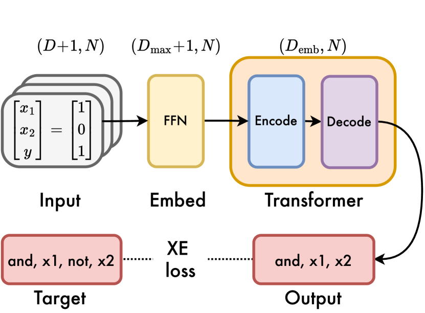
Figure 3: Summary of our approach. We feed $N$ points $(\bm{x},f(\bm{x}))\in\{0,1\}^{D+1}$ to a seq2seq Transformer, and supervise the prediction to $f$ via cross-entropy loss.

1.1 Contributions

1. We train Transformers over synthetic datasets to perform end-to-end symbolic regression of Boolean formulas and show that given the full truth table of an unseen function, the Boolformer is able to predict a compact formula, as illustrated in Fig. 1.

2. We show that Boolformer is robust to noisy and incomplete observations, by providing incomplete truth tables with flipped bits and irrelevant variables.

3. We evaluate Boolformer on various real-world binary classification tasks from the PMLB database [17] and show that it is competitive with classic machine learning approaches such as Random Forests while providing interpretable predictions, as illustrated in Fig. 3.

4. We apply Boolformer to the well-studied task of modelling gene regulatory networks (GRNs) in biology. Using a recent benchmark, we show that our model is competitive with state-of-the-art methods with several orders of magnitude faster inference.

5. Our code and models are available publicly at the following address:  https://github.com/sdascoli/boolformer. We also provide a pip package entitled boolformer for easy setup and usage.

1.2 Related work

Reasoning in deep learning

Several papers have studied the ability of deep neural networks to solve logic tasks. [18] introduce differential inductive logic as a method to learn logical rules from noisy data, and a few subsequent works attempted to craft dedicated neural architectures to improve this ability [19, 20, 21]. Large language models (LLMs) such as ChatGPT, however, have been shown to perform poorly at simple logical tasks such as basic arithmetic [22], and tend to rely on approximations and shortcuts [23]. Although some reasoning abilities seem to emerge with scale [24], achieving holistic and interpretable reasoning in LLMs remains an open challenge.

Boolean learnability

Leaning Boolean functions has been an active area in theoretical machine learning, mostly under the probably approximately correct (PAC) and statistical query (SQ) learning frameworks [25, 26]. More recently, [27] shows that regular neural networks learn by gradually fitting monomials of increasing degree, in such a way that the sample complexity is governed by the ‘leap complexity’ of the target function, i.e. the largest degree jump the Boolean function sees in its Fourier decomposition. In turn, [16] shows that this leads to a ‘min-degree bias’ limitation: Transformers tend to learn interpolators having least ‘degree profile’ in the Boolean Fourier basis, which typically lose the Boolean nature of the target and often produce complex solutions with poor out-of-distribution generalization.

Inferring Boolean formulas

A few works have explored the paradigm of inferring Boolean formulas from observations using SAT solvers [28], ILP solvers [29, 30] or via LP-relaxation [31]. However, all these works predict the formulas in conjunctive or disjunctive normal forms (CNF/DNF), which typically corresponds to exponentially long formulas. In contrast, the Boolformer is biased towards predicting compact expressions, which is more akin to logic synthesis – the task of finding the shortest circuit to express a given function, also known as the Minimum Circuit Size Problem (MCSP). While a few heuristics (e.g. Karnaugh maps [32]) and algorithms (e.g. ESPRESSO [33]) exist to tackle the MCSP, its NP-hardness [34] remains a barrier towards efficient circuit design. Given the high resilience of computers to errors, approximate logic synthesis techniques have been introduced [35, 36, 37, 38, 39, 40], with the aim of providing approximate expressions given incomplete data – this is similar in spirit to what we study in the noisy regime of Section 4.

Symbolic regression

Symbolic regression (SR), i.e. the search of mathematical expression underlying a set of numerical values, is still today a rather unexplored paradigm in the ML literature. Since this search cannot directly be framed as a differentiable problem, the dominant approach for SR is genetic programming (see [41] for a recent review). A few recent publications applied Transformer-based approaches to SR [42, 43, 44, 45], yielding comparable results but with a significant advantage: the inference time rarely exceeds a few seconds, several orders of magnitude faster than existing methods. Indeed, while the latter need to be run from scratch on each new set of observations, Transformers are trained over synthetic datasets, and inference simply consists in a forward pass.

2 Methods

Our task is to infer Boolean functions of the form $f:\{0,1\}^{D}\to\{0,1\}$, by predicting a Boolean formula built from the basic logical operators: AND, OR, NOT, as illustrated in Figs. 1,3. We train Transformers [1] on a large dataset of synthetic examples, following the seminal approach of [46]. For each example, the input $\mathcal{D}_{\mathrm{fit}}$ is a set of pairs $\{(\bm{x}_{i},y=f(\bm{x}_{i}))\}_{i=1\ldots N}$, and the target is the function $f$ as described above. Our general method is summarized in Fig. 3. Examples are generated by first sampling a random function $f$, then generating the corresponding $(\bm{x},y)$ pairs as described in the sections below.

2.1 Generating functions

We generate random Boolean formulas in the form of random unary-binary trees with mathematical operators as internal nodes and variables as leaves. The procedure is detailed as follows:

1. Sample the input dimension $D$ of the function $f$ uniformly in $[1,D_{\text{max}}]$ .

2. Sample the number of active variables $S$ uniformly in $[1,S_{\text{max}}]$. $S$ determines the number of variables which affect the output of $f$: the other variables are inactive. Then, select a set of $S$ variables from the original $D$ variables uniformly at random.

3. Sample the number of binary operators $B$ uniformly in $[S-1,B_{\text{max}}]$ then sample $B$ operators from {AND, OR} independently with equal probability.

4. Build a binary tree with those $B$ nodes, using the sampling procedure of [46], designed to produce a diverse mix of deep and narrow versus shallow and wide trees.

5. Negate some of the nodes of the tree by adding NOT gates independently with probability $p_{\text{NOT}}=\nicefrac{{1}}{{2}}$.

6. Fill in the leaves: for each of the $B+1$ leaves in the tree, sample independently and uniformly one of the variables from the set of active variables.

7. Simplify the tree using Boolean algebra rules, as described in App. A. This greatly reduces the number of operators, and occasionally reduces the number of active variables.

Note that the distribution of functions generated in this way spans the whole space of possible Boolean functions (which is of size $2^{2^{D}}$), but in a non-uniform fashion with a bias towards a controlled depth or width. To maximize diversity, we sample large formulas (up to $B_{\text{max}}=500$ binary gates), which are then heavily pruned in the simplification step. As discussed quantitatively in App. B, the diversity of functions generated in this way is such that throughout the whole training procedure, functions of dimension $D\geq 7$ are typically encountered at most once.

To represent Boolean formulas as sequences fed to the Transformer, we enumerate the nodes of the trees in prefix order, i.e., direct Polish notation as in [46]: operators and variables are represented as single autonomous tokens, e.g. $[\texttt{AND},x_{1},\texttt{NOT},x_{2}]$. The inputs are embedded using $\{\texttt{0},\texttt{1}\}$ tokens.

2.2 Generating inputs

Once the function $f$ is generated, we sample $N$ points $\bm{x}$ uniformly in the Boolean hypercube and compute the corresponding outputs $y=f(\bm{x})$. Optionally, we may flip the bits of the inputs and outputs independently with probability $\sigma_{\text{flip}}$; we consider the two following setups.

Noiseless regime

The noiseless regime, studied in Sec. 3, is defined as follows:

• Noiseless data: there is no bit flipping, i.e. $\sigma_{\text{flip}}=0$.

• Full support: all the input bits affect the output, i.e. $S=D$.

• Full observability: the model has access to the whole truth table of the Boolean function, i.e. $N=2^{D}$. Due to the quadratic length complexity of Transformers, this limits us to rather small input dimensions, i.e. $D_{\text{max}}=10$.

Noisy regime

In the noisy regime, studied in Sec. 4, the model must determine which variables affect the output, while also being able to cope with corruption of the inputs and outputs. During training, we vary the amount of noise for each sample so that the model can handle a variety of noise levels:

• Noisy data: the probability of each bit (both input and output) being flipped $\sigma_{\text{flip}}$ is sampled uniformly in $[0,0.1]$.

• Partial support: the model can handle high-dimensional functions, $D_{\text{max}}=120$, but the number of active variables is sampled uniformly in $[0,6]$. All the other variables are inactive.

• Partial observability: a subset of the hypercube is observed: the number of input points $N$ is sampled uniformly in $[30,300]$, which is typically much smaller that $2^{D}$. Additionally, instead of sampling uniformly (which would cause distribution shifts if the inputs are not uniformly distributed at inference), we generate the input points via a random walk in the hypercube. Namely, we sample an initial point $\bm{x}_{0}$ then construct the following points by flipping independently each coordinate with a probability $\gamma_{\text{expl}}$ sampled uniformly in $[0.05,0.25]$.

2.3 Model

Embedder

Our model is provided $N$ input points $(\bm{x},y)\in\{0,1\}^{D+1}$, each of which is represented by $D+1$ tokens of dimension $D_{\text{emb}}$. As $D$ and $N$ become large, this would result in very long input sequences (e.g. $10^{4}$ tokens for $D=100$ and $N=100$) which challenge the quadratic complexity of Transformers. To mitigate this, we introduce an embedder to map each input pair $(\bm{x},y)$ to a single embedding, following [44]. The embedder pads the empty input dimensions to $D_{\text{max}}$, enabling our model to handle variable input dimension, then concatenates all the tokens and feeds the $(D_{\text{max}}+1)D_{\text{emb}}$-dimensional result into a 2-layer fully-connected feedforward network (FFN) with ReLU activations, which projects down to dimension $D_{\text{emb}}$. The resulting $N$ embeddings of dimension $D_{\text{emb}}$ are then fed to the Transformer.

Transformer

We use a sequence-to-sequence Transformer architecture [1] where both the encoder and the decoder use 8 layers, 16 attention heads and an embedding dimension of 512, for a total of around 60M parameters (2M in the embedder, 25M in the encoder and 35M in the decoder). A notable property of this task is the permutation invariance of the $N$ input points. To account for this invariance, we remove positional embeddings from the encoder. The decoder uses standard learnable positional encodings.

2.4 Training and evaluation

Training

We optimize a cross-entropy loss with the Adam optimizer and a batch size of 128, warming up the learning rate from $10^{-7}$ to $2\times 10^{-4}$ over the first 10,000 steps, then decaying it using a cosine anneal for the next 300,000 steps, then restarting the annealing cycle with a damping factor of 3/2. We do not use any regularization, either in the form of weight decay or dropout. We train our models on around 30M examples; on a single NVIDIA A100 GPU with 80GB memory and 8 CPU cores, this takes about 3 days.

Inference

At inference time, we find that beam search is the best decoding strategy in terms of diversity and quality. In most results presented in this paper, we use a beam size of 10. One major advantage here is that we have an easy criterion to rank candidates, which is how well they fit the input data – to assess this, we use the fitting error defined in the following section. Note that when the data is noiseless, the model will often find several candidates which perfectly fit the inputs, as shown in App. LABEL:app:beam: in this case, we select the shortest formula, i.e. that with smallest number of gates.

Evaluation

Given a set of input-output pairs $\mathcal{D}$ generated by a target function $f_{\star}$, we compute the error of a predicted function $f$ as $\epsilon_{\mathcal{D}}=\frac{1}{|\mathcal{D}|}\sum_{(\bm{x},y)\in\mathcal{D}}1[f(\bm{x})=f_{\star}(\bm{x})]$. We can then define:

• Fitting error: error obtained when re-using the points used to predict the formula, $\mathcal{D}=\mathcal{D}_{\mathrm{fit}}$

• Fitting accuracy: defined as 1 if the fitting error is strictly equal to 0, and 0 otherwise.

• Test error: error obtained when sampling points uniformly at random in the hypercube outside of $\mathcal{D}_{\mathrm{fit}}$. Note that we can only assess this in the noisy regime, where the model observes a subset of the hypercube.

• Test accuracy: defined as 1 if the test error is strictly equal to 0, and 0 otherwise.

3 Noiseless regime: finding the shortest formula

We begin by the noiseless regime (see Sec. 2.2). This setting is akin to logic synthesis, where the goal is to find the shortest formula that implements a given function.

In-domain performance

In Fig. 4, we report the performance of the model when varying the number of input bits and the number of operators of the ground truth. Metrics are averaged over $10^{4}$ samples from the random generator; as demonstrated in App. B, these samples have typically not been seen during training for $D\geq 7$.

We observe that the model is able to recover the target function with high accuracy in all cases, even for $D\geq 7$ where memorization is impossible. We emphasize however that these results only quantify the performance of our model on the distribution of functions it was trained on, which is highly-nonuniform in the $2^{2^{D}}$-dimensional space of Boolean functions. We give a few examples of success and failure cases below.

Figure 4: Our model is able to recover the formula of unseen functions with high accuracy. We report the fitting error and accuracy of our model when varying the number of binary gates and input bits. Metrics are averaged over 10k samples from the random function generator.

Success and failure cases

In Fig. 1, we show two examples of Boolean functions where our model successfully predicts a compact formula for: the 4-to-1 multiplexer (which takes 6 input bits) and the 5-bit comparator (which takes 10 input bits). In App. D, we provide more examples: addition and multiplication, as well as majority and parity functions. By increasing the dimensionality of each problem up to the point of failure, we show that in all cases our model typically predicts exact and compact formulas as long as the function can be expressed with less than 50 binary gates (which is the largest size seen during training, as larger formulas exceed the 200 token limit) and fails beyond.

Hence, the failure point depends on the intrinsic difficulty of the function: for example, Boolformer can predict an exact formula for the comparator function up to $D=10$, but only $D=6$ for multiplication, $D=5$ for majority and $D=4$ for parity as well as typical random functions (whose outputs are independently sampled from $\{0,1\}$). Parity functions are well-known to be the most difficult functions to learn for SQ models due to their leap-complexity, are also the hardest to learn in our framework because they require the most operators to be expressed (the XOR operator being excluded in this work).

4 Noisy regime: applications to real-world data

We now turn to the noisy regime, which is defined at the end of Sec. 2.2. We begin by examining in-domain performance as before, then present two real-world applications: binary classification and gene regulatory network inference.

4.1 Results on noisy data

In Fig. 5, we show how the performance of our model depends on the various factors of difficulty of the problem. The different colors correspond to different numbers of active variables, as shown in the leftmost panel: in this setting with multiple sources of noise, we see that accuracy drops much faster with the number of active variables than in the noiseless setting.

As could be expected, performance improves as the number of input points $N$ increases, and degrades as the amount of random flipping and the number of inactive variables increase. However, the influence of the two latter parameters is rather mild, signalling that our model has an excellent ability to identify the support of the function and discard noise.

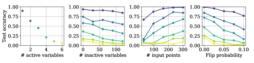
Figure 5: Our model is robust to data incompleteness, bit flipping and noisy variables. We display the error and accuracy of our model when varying the four factors of difficulty described in Sec. 2. The colors depict different number of active variables, as shown in the first panel. Metrics are averaged over 10k samples from the random generator.

4.2 Application to interpretable binary classification

In this section, we show that our noisy model can be applied to binary classification tasks, providing an interpretable alternative to classic machine learning methods on tabular data.

Method

We consider the tabular datasets from the Penn Machine Learning Benchmark (PMLB) from [17]. These encapsulate a wide variety of real-world problems such as predicting chess moves, toxicity of mushrooms, credit scores and heart diseases. Since our model can only take binary features as input, we discard continuous features, and binarize the categorical features with $C>2$ classes into $C$ binary variables. Note that this procedure can greatly increase the total number of features – we only keep datasets for which it results in less than 120 features (the maximum our model can handle). We randomly sample $25\%$ of the examples for testing and report the F1 score obtained on this held out set.

We compare our model with two classic machine learning methods: logistic regression and random forests, using the default hyperparameters from sklearn. For random forests, we test two values for the number of estimators: 1 (in which case we obtain a simple decision tree as for the boolformer) and 100.

Results

Results are reported in Fig. 6, where for readability we only display the datasets where the RandomForest with 100 estimators achieves an F1 score above 0.75. The performance of the Boolformer is similar on average to that of logistic regression: logistic regression typically performs better on "hard" datasets where there is no exact logical rule, for example medical diagnosis tasks such as heart_h, but worse on logic-based datasets where the data is not linearly separable such as xd6.

The F1 score of our model is slightly below that of a random forest of 100 trees, but slightly above that of the random forest with a single tree. This is remarkable considering that the Boolean formula it outputs only contains a few dozen nodes at most, whereas the trees of random forest use up to several hundreds. We show an example of a Boolean formula predicted for the mushroom toxicity dataset in Fig. 3, and a more extensive collection of formulas in App. LABEL:app:pmlb.

Figure 6: Our model is competitive with classic machine learning methods while providing highly interpretable results. We display the F1 score obtained on various binary classification datasets from the Penn Machine Learning Benchmark [17]. We compare the F1 score of the Boolformer with random forests (using 1 and 100 estimators) and logistic regression, using the default settings of sklearn, and display the average F1 score of each method in the legend.

4.3 Inferring Boolean networks: application to gene regulatory networks

A Boolean network is a dynamical system composed of $D$ bits whose transition from one state to the next is governed by a set of $D$ Boolean functions. These types of networks have attracted a lot of attention in the field of computational biology as they can be used to model gene regulatory networks (GRNs) [47] – see App. LABEL:app:grn for a brief overview of this field. In this setting, each bit represents the (discretized) expression of a gene (on or off) and each function represents the regulation of a gene by the other genes. In this section, we investigate the applicability of our symbolic regression-based approach to this task.

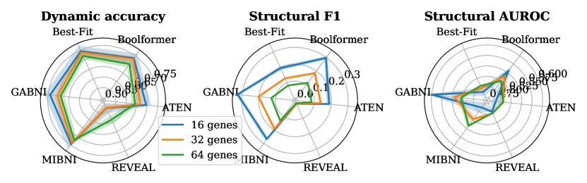
(a) Dynamic and structural metrics

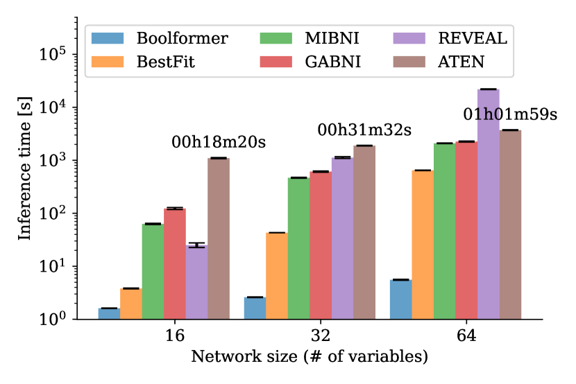
(b) Average inference time

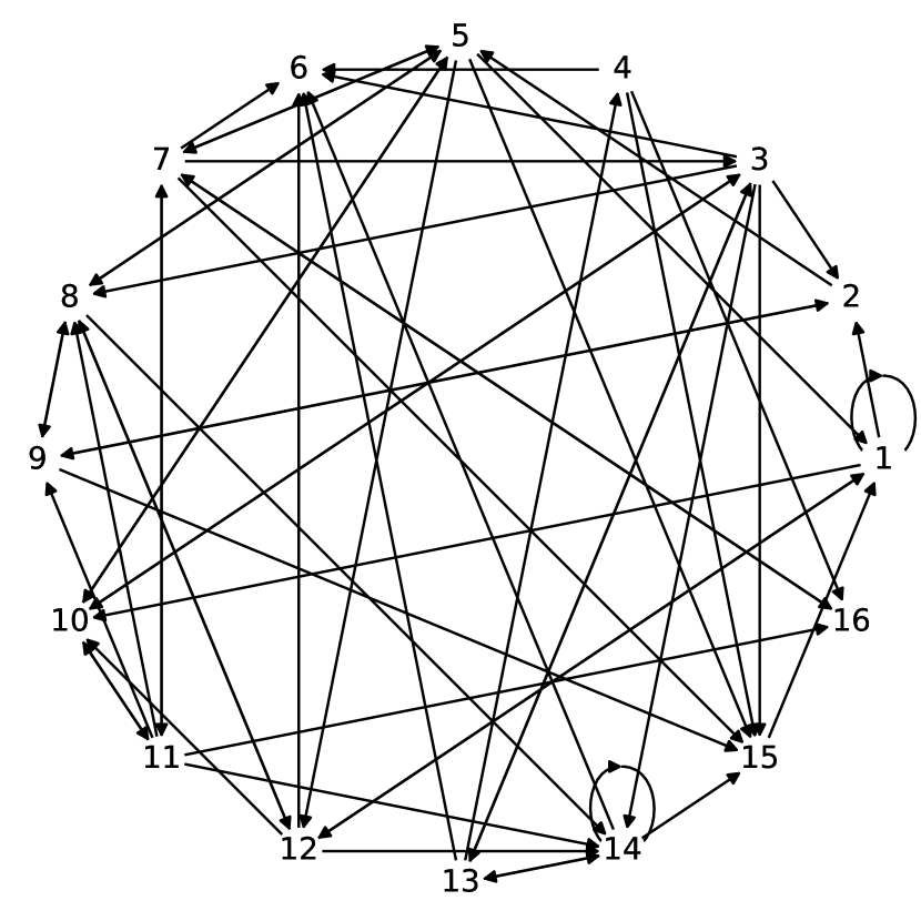
(c) Example of a GRN inferred

Figure 7: Our model is competitive with state-of-the-art methods for GRN inference with orders of magnitude faster inference. (a) We compare the ability of our model to predict the next states (dynamic accuracy) and the influence graph (structural accuracy) with that of other methods using a recent benchmark [48] – more details in Sec. 4.3. (b) Average inference time of the various methods. (c) From the Boolean formulas predicted, one can construct an influence graph where each node represents a gene, and each arrow signals that one gene regulates another.

Benchmark

We use the recent benchmark for GRN inference introduced by [48]. This benchmark compares 5 methods for Boolean network inference on 30 Boolean networks inferred from biological data, with sizes ranging from 16 to 64 genes, and assesses both dynamical prediction (how well the model predicts the dynamics of the network) and structural prediction (how well the model predicts the Boolean functions compared to the ground truth). Structural prediction is framed as the binary classification task of predicting whether variable $i$ influences variable $j$, and can hence be evaluated by many binary classification metrics; we report here the structural F1 and the AUROC metrics which are the most holistic, and defer other metrics to App. LABEL:app:grn.

Method

Our model predicts each component $f_{i}$ of the Boolean network independently, by taking as input the whole state of the network at times $[0\ldots t-1]$ and as output the state of the $i$th bit at times $[1\ldots t]$. Once each component has been predicted, we can build a causal influence graph, where an arrow connects node $i$ to node $j$ if $j$ appears in the update equation of $i$: an example is shown in Fig. 7c. Note that since the dynamics of the Boolean network tend to be slow, an easy way to get rather high dynamical accuracy would be to simply predict the trivial fixed point $f_{i}=x_{i}$. In concurrent approaches, the function set explored excludes this solution; in our case, we simply mask the $i$th bit from the input when predicting $f_{i}$.

Results

We display the results of our model on the benchmark in Fig. 7a. The Boolformer performs on par with the SOTA algorithms, GABNI [49] and MIBNI [50]. A striking feature of our model is its inference speed, displayed in Fig. 7b: a few seconds, against up to an hour for concurrent approaches, which mainly rely on genetic programming. Note also that our model predicts an interpretable Boolean function, whereas the other SOTA methods (GABNI and MIBNI) simply pick out the most important variables and the sign of their influence.

5 Discussion and limitations

In this work, we have shown that Transformers excel at symbolic regression of logical functions, both in the noiseless setup where they could potentially provide valuable insights for circuit design, and in the real-world setup of binary classification where they can provide interpretable solutions. Their ability to infer GRNs several orders of magnitude faster than existing methods offers the promise of many other exciting applications in biology, where Boolean modelling plays a key role [15]. There are however several limitations in our current approach, which open directions for future work.

First, due to the quadratic cost of self-attention, the number of input points is limited to a thousand during training, which limits the model’s performance on high-dimensional functions and large datasets (although the model does exhibit some length generalization abilities at inference, as shown in App. C). One could address this shortcoming with linear attention mechanisms [51, 52], at the risk of degrading performance.

Second, the logical functions which our model is trained on do not include the XOR gate explicitly, limiting both the compactness of the formulas it predicts and its ability to express complex formulas such as parity functions. The reason for this limitation is that our generation procedure relies on expression simplification, which requires rewriting the XOR gate in terms of AND, OR and NOT. We leave it as a future work to adapt the generation of simplified formulas containing XOR gates, as well as operators with higher parity as in [40].

Third, the simplicity of the formulas predicted is limited in two additional ways: our model only handles (i) single-output functions – multi-output functions are predicted independently component-wise and (ii) gates with a fan-out of one. As a result, our model cannot reuse intermediary results for different outputs or for different computations within a single output. One could address this either by post-processing the generated formulas to identify repeated substructures, or by adapting the data generation process to support multi-output functions (a rather easy extension) and cyclic graphs (which would require more work).

Finally, this paper mainly focused on investigating concrete applications and benchmarks to motivate the potential and development of Boolformers. In future research, we will tackle various theoretical aspects of this paradigm, such as the model simplicity bias, the sample complexity and the ‘generalization on the unseen’ [27] of the Boolformer, comparing with other existing methods for Boolean learning.

Appendix A Expression simplification

The data generation procedure heavily relies on expression simplification. This is of utmost importance for four reasons:

• It reduces the output expression length and hence memory usage as well as increasing speed

• It improves the supervision by reducing expressions to a more canonical form, easier to guess for the model

• It increases the effective diversity of the beam search, by reducing the number of equivalent expressions generated

• It encourages the model to output the simplest formula, which is a desirable property.

We use the package boolean.py for this, which is considerably faster than sympy (the function simplify_logic of the latter has exponential complexity, and is hence only implemented for functions with less then 9 input variables).

Empirically, we found the following procedure to be optimal in terms of average length obtained after simplification:

1. Preprocess the formula by applying basic logical equivalences: double negation elimination and De Morgan’s laws.

2. Parse the formula with boolean.py and run the simplify() method twice

3. Apply once again the first step

Note that this procedure drastically reduces the number of operators and renders the final distribution highly nonuniform, as shown in Fig. 8.

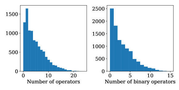
Figure 8: Distribution of number of operators after expression simplification. The initial number of binary operators is sampled uniformly in [1, 1000]. The total number of examples is $10^{4}$.

Appendix B Does the Boolformer memorize?

One natural question is whether our model simply performs memorization on the training set. Indeed, the number of possible functions of $D$ variables is finite, and equal to $2^{2^{D}}$.

Let us first assume naively that our generator is uniform in the space of boolean functions. Since $2^{2^{4}}\simeq 6\times 10^{4}$ (which is smaller than the number of examples seen during training) and $2^{2^{5}}\simeq 5.10^{9}$ (which is much larger), one could conclude that for $D\leq 4$, all functions are memorized, whereas for $D>4$, only a small subset of all possible functions are seen, hence memorization cannot occur.

However, the effective number of unique functions seen during training is actually smaller because our generator of random functions is nonuniform in the space of boolean functions. In this case, for which value of $D$ does memorization become impossible? To investigate this question, for each $D<D_{\text{max}}$, we sample $\min\left(2^{2^{D}},100\right)$ unique functions from our random generator, and count how many times their exact truth table is encountered over an epoch (300,000 examples).

Results are displayed in Fig. 9. As expected, the average number of occurences of each function decays exponentially fast, and falls to zero for $D=7$, meaning that each function is typically unique for $D\geq 7$. Hence, memorization cannot occur for $D\geq 7$. Yet, as shown in Fig. 4, our model achieves excellent accuracies even for functions of 10 variables, which excludes memorization as a possible explanation for the ability of our model to predict logical formulas accurately.

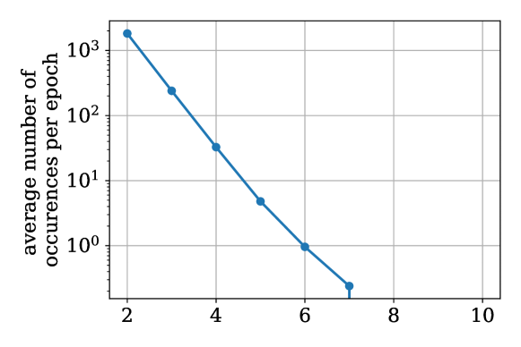
Figure 9: Functions with 7 or more variables are typically never seen more than once during training. We display the average number of times functions of various input dimensionalities are seen during an epoch (300,000 examples). For each point on the curve, the average is taken over $\min(2^{2^{D}}),100)$ unique functions.

Appendix C Length generalization

In this section we examine the ability of our model to length generalize. In this setting, there are two types of generalization one can define: generalization in terms of the number of inputs $N$, or in terms of the number of active variables $S$. We examine length generalization in the noisy setup (see Sec. 2.2), because in the noiseless setup, the model already has access to all the truth table (increasing $N$ does not bring any extra information), and all the variables are active (we cannot increase $S$ as it is already equal to $D$).

C.1 Number of inputs

Since the input points fed to the model are permutation invariant, our model does not use any positional embeddings. Hence, not only can our model handle $N>N_{\text{max}}$, but performance often continues to improve beyond $N_{\text{max}}$, as we show for two datasets extracted from PMLB [17] in Fig. 10.

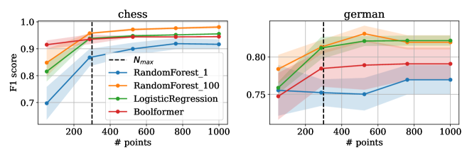
Figure 10: Our model can length generalize in terms of sequence length. We test a model trained with $N_{\text{max}}=300$ on the chess and german datasets of PMLB. Results are averaged over 10 random samplings of the input points, with the shaded areas depicting the standard deviation.

C.2 Number of variables

To assess whether our model can infer functions which contain more active variables than seen during training, we evaluated a model trained on functions with up to 6 active variables on functions with 7 or more active variables. We provided the model with the truth table of two very simply functions: the OR and AND of the first $S\geq 7$ variables. We observe that the model succeeds for $S=7$, but fails for $S\geq 8$, where it only includes the first 7 variables in the OR / AND. Hence, the model can length generalize to a small extent in terms of number of active variables, but less easily than in terms of number of inputs. We hypothesize that proper length generalization could be achieved by "priming", i.e. adding even a small number of "long" examples, as performed in [22].

Appendix D Formulas predicted for logical circuits

In Figs. LABEL:fig:arithmetic-formulas and LABEL:fig:logical_formulas, we show examples of some common arithmetic and logical formulas predicted by our model in the noiseless regime, with a beam size of 100. In all cases, we increase the dimensionality of the problem until the failure point of the Boolformer.

[$y_{0}$ [$\mathrm{and}$ [$x_{0}$ ][$x_{1}$ ][$x_{2}$ ][$x_{3}$ ]]] [$y_{2}$ [$\mathrm{and}$ [$\mathrm{or}$ [$x_{0}$ ][$x_{2}$ ][$\mathrm{and}$ [$x_{1}$ ][$x_{3}$ ]]][$\mathrm{not}$ [$\mathrm{and}$ [$x_{0}$ ][$x_{1}$ ][$x_{2}$ ][$x_{3}$ ]]][$\mathrm{or}$ [$x_{1}$ ][$x_{3}$ ][$\mathrm{and}$ [$x_{0}$ ][$x_{2}$ ]]]]] [$y_{1}$ [$\mathrm{not}$ [$\mathrm{or}$ [$\mathrm{and}$ [$x_{0}$ ][$x_{1}$ ][$x_{2}$ ][$x_{3}$ ]][$\mathrm{and}$ [$\mathrm{not}$ [$x_{0}$ ]][$x_{1}$ ][$x_{2}$ ][$\mathrm{not}$ [$x_{3}$ ]]][$\mathrm{and}$ [$x_{1}$ ][$\mathrm{not}$ [$x_{2}$ ]][$\mathrm{or}$ [$x_{0}$ ][$x_{3}$ ]][$\mathrm{not}$ [$\mathrm{and}$ [$x_{0}$ ][$x_{3}$ ]]]][$\mathrm{and}$ [$\mathrm{not}$ [$x_{1}$ ]][$\mathrm{or}$ [$x_{0}$ ][$x_{2}$ ][$\mathrm{not}$ [$x_{3}$ ]]][$\mathrm{or}$ [$\mathrm{not}$ [$x_{0}$ ]][$x_{2}$ ][$x_{3}$ ]][$\mathrm{or}$ [$\mathrm{not}$ [$x_{2}$ ]][$\mathrm{and}$ [$x_{0}$ ][$\mathrm{not}$ [$x_{3}$ ]]][$\mathrm{and}$ [$\mathrm{not}$ [$x_{0}$ ]][$x_{3}$ ]]]]]]]

(a) Addition of four bits: $y_{0}y_{1}y_{2}=x_{0}+x_{1}+x_{2}+x_{3}$. All formulas are correct.

[$y_{0}$ [$\mathrm{or}$ [$\mathrm{and}$ [$x_{0}$ ][$x_{2}$ ][$x_{3}$ ][$\mathrm{or}$ [$x_{1}$ ][$x_{4}$ ]]][$\mathrm{and}$ [$x_{1}$ ][$x_{4}$ ][$\mathrm{or}$ [$x_{0}$ ][$x_{2}$ ]][$\mathrm{or}$ [$x_{3}$ ][$\mathrm{and}$ [$x_{0}$ ][$x_{2}$ ]]]]]] [$y_{1}$ [$\mathrm{not}$ [$\mathrm{and}$ [$\mathrm{or}$ [$x_{0}$ ][$\mathrm{not}$ [$x_{1}$ ]][$x_{2}$ ][$\mathrm{not}$ [$\mathrm{and}$ [$x_{3}$ ][$x_{4}$ ]]]][$\mathrm{or}$ [$\mathrm{not}$ [$x_{0}$ ]][$\mathrm{not}$ [$x_{1}$ ]][$x_{2}$ ][$x_{3}$ ][$\mathrm{not}$ [$x_{4}$ ]]][$\mathrm{or}$ [$x_{1}$ ][$x_{2}$ ][$x_{3}$ ][$x_{4}$ ][$\mathrm{not}$ [$\mathrm{or}$ [$x_{0}$ ][$\mathrm{and}$ [$x_{3}$ ][$x_{4}$ ]]]]][$\mathrm{or}$ [$x_{2}$ ][$\mathrm{not}$ [$x_{3}$ ]][$x_{4}$ ][$\mathrm{and}$ [$x_{0}$ ][$\mathrm{not}$ [$x_{1}$ ]]][$\mathrm{and}$ [$\mathrm{not}$ [$x_{0}$ ]][$x_{1}$ ]]][$\mathrm{or}$ [$\mathrm{not}$ [$x_{2}$ ]][$\mathrm{and}$ [$x_{0}$ ][$\mathrm{not}$ [$x_{1}$ ]][$x_{3}$ ][$x_{4}$ ]][$\mathrm{and}$ [$\mathrm{not}$ [$x_{0}$ ]][$\mathrm{not}$ [$x_{1}$ ]][$x_{3}$ ][$\mathrm{not}$ [$x_{4}$ ]]][$\mathrm{and}$ [$x_{1}$ ][$x_{3}$ ][$x_{4}$ ]][$\mathrm{and}$ [$\mathrm{not}$ [$x_{3}$ ]][$\mathrm{or}$ [$x_{0}$ ][$\mathrm{not}$ [$\mathrm{and}$ [$x_{1}$ ][$x_{4}$ ]]]][$\mathrm{or}$ [$\mathrm{not}$ [$x_{2}$ ]][$x_{4}$ ][$\mathrm{and}$ [$\mathrm{not}$ [$x_{0}$ ]][$x_{1}$ ]]]]]]]] [$y_{2}$ [$\mathrm{not}$ [$\mathrm{or}$ [$\mathrm{and}$ [$x_{0}$ ][$x_{2}$ ][$x_{3}$ ][$\mathrm{or}$ [$x_{1}$ ][$x_{4}$ ]]][$\mathrm{not}$ [$\mathrm{or}$ [$x_{0}$ ][$x_{1}$ ][$x_{3}$ ][$\mathrm{and}$ [$x_{2}$ ][$x_{4}$ ]]]][$\mathrm{and}$ [$x_{1}$ ][$x_{2}$ ][$x_{4}$ ][$\mathrm{or}$ [$x_{0}$ ][$x_{3}$ ]]][$\mathrm{not}$ [$\mathrm{or}$ [$x_{2}$ ][$x_{4}$ ][$\mathrm{and}$ [$x_{0}$ ][$x_{1}$ ]][$\mathrm{and}$ [$x_{3}$ ][$\mathrm{or}$ [$x_{0}$ ][$x_{1}$ ]]]]]]]]

(b) Addition of five bits: $y_{0}y_{1}y_{2}=x_{0}+x_{1}+x_{2}+x_{3}+x_{4}$. The first formula is correct, the second gets 20% error, the last 3% error.

[$y_{0}$ [$\mathrm{or}$ [$\mathrm{and}$ [$x_{0}$ ][$x_{2}$ ]][$\mathrm{and}$ [$x_{1}$ ][$x_{3}$ ][$\mathrm{or}$ [$x_{0}$ ][$x_{2}$ ]]]]] [$y_{1}$ [$\mathrm{and}$ [$\mathrm{or}$ [$x_{1}$ ][$x_{3}$ ]][$\mathrm{not}$ [$\mathrm{and}$ [$x_{1}$ ][$x_{3}$ ]]]]] [$y_{2}$ [$\mathrm{and}$ [$\mathrm{or}$ [$x_{0}$ ][$\mathrm{not}$ [$\mathrm{and}$ [$x_{1}$ ][$x_{2}$ ][$x_{3}$ ]]]][$\mathrm{or}$ [$\mathrm{and}$ [$x_{0}$ ][$\mathrm{not}$ [$\mathrm{or}$ [$x_{2}$ ][$\mathrm{and}$ [$x_{1}$ ][$x_{3}$ ]]]]][$\mathrm{and}$ [$\mathrm{not}$ [$x_{0}$ ]][$x_{2}$ ]][$\mathrm{and}$ [$x_{1}$ ][$x_{3}$ ][$\mathrm{or}$ [$\mathrm{not}$ [$x_{0}$ ]][$x_{2}$ ]]]]]]

(a) Addition of two 2-bit numbers: $y_{0}y_{1}y_{2}=(x_{0}x_{1})+(x_{2}x_{3})$. All formulas are correct.

References

- [1] Ashish Vaswani et al. “Attention is all you need” In Advances in neural information processing systems, 2017, pp. 5998–6008
- [2] Alexey Dosovitskiy et al. “An image is worth 16x16 words: Transformers for image recognition at scale” In arXiv preprint arXiv:2010.11929, 2020
- [3] Tom Brown et al. “Language Models are Few-Shot Learners” In Advances in Neural Information Processing Systems 33 Curran Associates, Inc., 2020, pp. 1877–1901 URL: https://proceedings.neurips.cc/paper_files/paper/2020/file/1457c0d6bfcb4967418bfb8ac142f64a-Paper.pdf
- [4] John Jumper et al. “Highly accurate protein structure prediction with AlphaFold” In Nature 596.7873 Nature Publishing Group UK London, 2021, pp. 583–589
- [5] Grégoire Delétang et al. “Neural networks and the chomsky hierarchy” In arXiv preprint arXiv:2207.02098, 2022
- [6] David Saxton, Edward Grefenstette, Felix Hill and Pushmeet Kohli “Analysing mathematical reasoning abilities of neural models” In arXiv preprint arXiv:1904.01557, 2019
- [7] Aitor Lewkowycz et al. “Solving quantitative reasoning problems with language models” In Advances in Neural Information Processing Systems 35, 2022, pp. 3843–3857
- [8] Petar Veličković et al. “The CLRS algorithmic reasoning benchmark” In International Conference on Machine Learning, 2022, pp. 22084–22102 PMLR
- [9] Yi Zhang et al. “Unveiling transformers with lego: a synthetic reasoning task” In arXiv preprint arXiv:2206.04301, 2022
- [10] Chiyuan Zhang, Maithra Raghu, Jon Kleinberg and Samy Bengio “Pointer value retrieval: A new benchmark for understanding the limits of neural network generalization” In arXiv preprint arXiv:2107.12580, 2021
- [11] Justin Johnson et al. “Clevr: A diagnostic dataset for compositional language and elementary visual reasoning” In Proceedings of the IEEE conference on computer vision and pattern recognition, 2017, pp. 2901–2910
- [12] Jian Liu et al. “Logiqa: A challenge dataset for machine reading comprehension with logical reasoning” In arXiv preprint arXiv:2007.08124, 2020
- [13] Karl Cobbe et al. “Training verifiers to solve math word problems” In arXiv preprint arXiv:2110.14168, 2021
- [14] Rui-Sheng Wang, Assieh Saadatpour and Reka Albert “Boolean modeling in systems biology: an overview of methodology and applications” In Physical biology 9.5 IOP Publishing, 2012, pp. 055001
- [15] Ahmed Abdelmonem Hemedan, Anna Niarakis, Reinhard Schneider and Marek Ostaszewski “Boolean modelling as a logic-based dynamic approach in systems medicine” In Computational and Structural Biotechnology Journal 20 Elsevier, 2022, pp. 3161–3172
- [16] Emmanuel Abbe et al. “Learning to reason with neural networks: Generalization, unseen data and boolean measures” In arXiv preprint arXiv:2205.13647, 2022
- [17] Randal S. Olson et al. “PMLB: a large benchmark suite for machine learning evaluation and comparison” In BioData Mining 10.1, 2017, pp. 36 DOI: 10.1186/s13040-017-0154-4
- [18] Richard Evans and Edward Grefenstette “Learning explanatory rules from noisy data” In Journal of Artificial Intelligence Research 61, 2018, pp. 1–64
- [19] Gabriele Ciravegna et al. “Logic explained networks” In Artificial Intelligence 314 Elsevier, 2023, pp. 103822
- [20] Shaoyun Shi et al. “Neural logic reasoning” In Proceedings of the 29th ACM International Conference on Information & Knowledge Management, 2020, pp. 1365–1374
- [21] Honghua Dong et al. “Neural logic machines” In arXiv preprint arXiv:1904.11694, 2019
- [22] Samy Jelassi et al. “Length Generalization in Arithmetic Transformers” In arXiv preprint arXiv:2306.15400, 2023
- [23] Bingbin Liu et al. “Transformers learn shortcuts to automata” In arXiv preprint arXiv:2210.10749, 2022
- [24] Jason Wei et al. “Emergent Abilities of Large Language Models”, 2022 arXiv:2206.07682 [cs.CL]
- [25] Lisa Hellerstein and Rocco A Servedio “On pac learning algorithms for rich boolean function classes” In Theoretical Computer Science 384.1 Elsevier, 2007, pp. 66–76
- [26] Lev Reyzin “Statistical queries and statistical algorithms: Foundations and applications” In arXiv preprint arXiv:2004.00557, 2020
- [27] Emmanuel Abbe, Enric Boix-Adsera and Theodor Misiakiewicz “SGD learning on neural networks: leap complexity and saddle-to-saddle dynamics” In arXiv preprint arXiv:2302.11055, 2023
- [28] Nina Narodytska et al. “Learning Optimal Decision Trees with SAT.” In Ijcai, 2018, pp. 1362–1368
- [29] Tong Wang and Cynthia Rudin “Learning optimized Or’s of And’s” In arXiv preprint arXiv:1511.02210, 2015
- [30] Guolong Su, Dennis Wei, Kush R Varshney and Dmitry M Malioutov “Interpretable two-level boolean rule learning for classification” In arXiv preprint arXiv:1511.07361, 2015
- [31] Dmitry M Malioutov, Kush R Varshney, Amin Emad and Sanjeeb Dash “Learning interpretable classification rules with boolean compressed sensing” In Transparent Data Mining for Big and Small Data Springer, 2017, pp. 95–121
- [32] Maurice Karnaugh “The map method for synthesis of combinational logic circuits” In Transactions of the American Institute of Electrical Engineers, Part I: Communication and Electronics 72.5 IEEE, 1953, pp. 593–599
- [33] Richard L Rudell and Alberto Sangiovanni-Vincentelli “Multiple-valued minimization for PLA optimization” In IEEE Transactions on Computer-Aided Design of Integrated Circuits and Systems 6.5 IEEE, 1987, pp. 727–750
- [34] Cody D Murray and R Ryan Williams “On the (non) NP-hardness of computing circuit complexity” In Theory of Computing 13.1 Theory of Computing Exchange, 2017, pp. 1–22
- [35] Ilaria Scarabottolo, Giovanni Ansaloni and Laura Pozzi “Circuit carving: A methodology for the design of approximate hardware” In 2018 Design, Automation & Test in Europe Conference & Exhibition (DATE), 2018, pp. 545–550 IEEE
- [36] Swagath Venkataramani et al. “SALSA: Systematic logic synthesis of approximate circuits” In Proceedings of the 49th Annual Design Automation Conference, 2012, pp. 796–801
- [37] Swagath Venkataramani, Kaushik Roy and Anand Raghunathan “Substitute-and-simplify: A unified design paradigm for approximate and quality configurable circuits” In 2013 Design, Automation & Test in Europe Conference & Exhibition (DATE), 2013, pp. 1367–1372 IEEE
- [38] Sina Boroumand, Christos-Savvas Bouganis and George A Constantinides “Learning boolean circuits from examples for approximate logic synthesis” In Proceedings of the 26th Asia and South Pacific Design Automation Conference, 2021, pp. 524–529
- [39] Arlindo Oliveira and Alberto Sangiovanni-Vincentelli “Learning complex boolean functions: Algorithms and applications” In Advances in Neural Information Processing Systems 6, 1993
- [40] Gili Rosenberg et al. “Explainable AI using expressive Boolean formulas” In arXiv preprint arXiv:2306.03976, 2023
- [41] William La Cava et al. “Contemporary symbolic regression methods and their relative performance” In arXiv preprint arXiv:2107.14351, 2021
- [42] Luca Biggio et al. “Neural Symbolic Regression that Scales”, 2021 arXiv:2106.06427 [cs.LG]
- [43] Mojtaba Valipour, Bowen You, Maysum Panju and Ali Ghodsi “SymbolicGPT: A Generative Transformer Model for Symbolic Regression” In arXiv preprint arXiv:2106.14131, 2021
- [44] Pierre-Alexandre Kamienny, Stéphane d’Ascoli, Guillaume Lample and Francois Charton “End-to-end Symbolic Regression with Transformers” In Advances in Neural Information Processing Systems, 2022 URL: https://openreview.net/forum?id=GoOuIrDHG_Y
- [45] Wassim Tenachi, Rodrigo Ibata and Foivos I Diakogiannis “Deep symbolic regression for physics guided by units constraints: toward the automated discovery of physical laws” In arXiv preprint arXiv:2303.03192, 2023
- [46] Guillaume Lample and François Charton “Deep learning for symbolic mathematics” In arXiv preprint arXiv:1912.01412, 2019
- [47] Mengyuan Zhao et al. “A comprehensive overview and critical evaluation of gene regulatory network inference technologies” In Briefings in Bioinformatics 22.5 Oxford University Press, 2021, pp. bbab009
- [48] Žiga Pušnik, Miha Mraz, Nikolaj Zimic and Miha Moškon “Review and assessment of Boolean approaches for inference of gene regulatory networks” In Heliyon Elsevier, 2022, pp. e10222
- [49] Shohag Barman and Yung-Keun Kwon “A Boolean network inference from time-series gene expression data using a genetic algorithm” In Bioinformatics 34.17 Oxford University Press, 2018, pp. i927–i933
- [50] Shohag Barman and Yung-Keun Kwon “A novel mutual information-based Boolean network inference method from time-series gene expression data” In PloS one 12.2 Public Library of Science San Francisco, CA USA, 2017, pp. e0171097
- [51] Krzysztof Choromanski et al. “Rethinking attention with performers” In arXiv preprint arXiv:2009.14794, 2020
- [52] Sinong Wang et al. “Linformer: Self-attention with linear complexity” In arXiv preprint arXiv:2006.04768, 2020
- [53] Nitin Singh and Mathukumalli Vidyasagar “bLARS: An algorithm to infer gene regulatory networks” In IEEE/ACM transactions on computational biology and bioinformatics 13.2 IEEE, 2015, pp. 301–314
- [54] Anne-Claire Haury, Fantine Mordelet, Paola Vera-Licona and Jean-Philippe Vert “TIGRESS: trustful inference of gene regulation using stability selection” In BMC systems biology 6.1 BioMed Central, 2012, pp. 1–17
- [55] Vân Anh Huynh-Thu, Alexandre Irrthum, Louis Wehenkel and Pierre Geurts “Inferring regulatory networks from expression data using tree-based methods” In PloS one 5.9 Public Library of Science San Francisco, USA, 2010, pp. e12776
- [56] Emmanuel S Adabor and George K Acquaah-Mensah “Restricted-derestricted dynamic Bayesian Network inference of transcriptional regulatory relationships among genes in cancer” In Computational biology and chemistry 79 Elsevier, 2019, pp. 155–164
- [57] Vân Anh Huynh-Thu and Pierre Geurts “dynGENIE3: dynamical GENIE3 for the inference of gene networks from time series expression data” In Scientific reports 8.1 Nature Publishing Group UK London, 2018, pp. 3384
- [58] Shoudan Liang, Stefanie Fuhrman and Roland Somogyi “Reveal, a general reverse engineering algorithm for inference of genetic network architectures” In Biocomputing 3, 1998
- [59] Harri Lähdesmäki, Ilya Shmulevich and Olli Yli-Harja “On learning gene regulatory networks under the Boolean network model” In Machine learning 52.1-2 Springer Nature BV, 2003, pp. 147
- [60] Ning Shi et al. “ATEN: And/Or tree ensemble for inferring accurate Boolean network topology and dynamics” In Bioinformatics 36.2 Oxford University Press, 2020, pp. 578–585