Suppression of Neutron Background using Deep Neural Network and Fourier Frequency Analysis at the KOTO Experiment
Abstract
We present two analysis techniques for distinguishing background events induced by neutrons from photon signal events in the search for the rare decay at the J-PARC KOTO experiment. These techniques employed a deep convolutional neural network and Fourier frequency analysis to discriminate neutrons from photons, based on their variations in cluster shape and pulse shape, in the electromagnetic calorimeter made of undoped CsI. The results effectively suppressed the neutron background by a factor of , while maintaining the efficiency of at .
keywords:
Rare kaon decay , Convolutional neural network , Deep learning , Cluster shape discrimination , Pulse shape discrimination , Fourier frequency analysis.[chicago]organization=Enrico Fermi Institute,addressline=University of Chicago, city=Chicago, postcode=60637, state=Illinois, country=USA
[taiwan]organization=Department of Physics,addressline=National Taiwan University, city=Taipei, postcode=10617, country=Taiwan, Republic of China
[osaka]organization=Department of Physics,addressline=Osaka University, Toyonaka, city=Osaka, postcode=560-0043, country=Japan
[kek]organization=Institute of Particle and Nuclear Studies,addressline=High Energy Accelerator Research Organization (KEK), city=Tsukuba, postcode=305-0801, state=Ibaraki, country=Japan
[kyoto]organization=Department of Physics,addressline=Kyoto University, city=Kyoto, postcode=606-8502, country=Japan
1 Introduction
The KOTO experiment at J-PARC was designed to search for the rare decay of , which has a theoretical branching ratio of in the standard model [1]. The current result on the measurement is an experimental upper limit on the branching ratio, which is at the confidence level set by KOTO [2, 3]. KOTO utilized the high-intensity proton beam incident on a gold target to produce secondary particles, and the secondary neutral particles, including kaons, were guided to the KOTO detector by two sets of collimators [4]. The only visible products in the decay are two photons from the subsequent decay of . Therefore, a event is identified by two photons detected in a Cesium Iodide crystal calorimeter (CSI) [5]. One of the dominant background sources in the search for was the beam-halo neutron. These neutrons could present a similar event signature with two photon-like hits in the CSI. A halo neutron background event was caused by a single halo neutron particle that interacted inside the CSI and produced two photon-like hits. Typically, the first hit occurred near the neutron’s incident point on the CSI, while the second hit, produced by the same neutron after the scattering process, was separated from the first hit by some distance. These two hits in the CSI with no trace in between could be mistaken as the two isolated photon hits from . Suppressing the halo neutron background relied on distinguishing the interaction footprints of photon and neutron hits in the CSI, which were characterized by differences in the incident particle’s cluster shape and pulse shape in the CSI.
The CSI consisted of 2716 Cesium Iodide (CsI) crystals arranged in a grid format with each crystal having its own individual readout. When a particle interacted with the CSI, the analog pulse shape in each crystal was digitized and recorded, and the cluster shape was formed by grouping nearby CsI crystals with deposited energy by the incident particle. Discrimination between photons and neutrons was based on variations in cluster shape and pulse shape. Although the cluster shape discrimination [5] and the pulse shape discrimination [6] had been previously studied at KOTO, in this article, we introduce two new techniques: using a Convolutional Neural Network (CNN) [8] to classify cluster shapes (Section 3) and Fourier frequency analysis to discriminate pulse shapes (Section 4). In addition, we introduce a more precise method for estimating the neutron background level in Section 5. These techniques were first introduced to the analysis of the data obtained from the years 2016–2018 [3], and the result further suppressed KOTO’s dominant background source, the halo neutron, by a factor of 26 over the previous analysis result of 2015 data [2]. This article provides a detailed explanation of how neutron background events were suppressed and estimated in the 2016–2018 data analysis, which was not presented in the previous publications of KOTO.
2 CsI detector
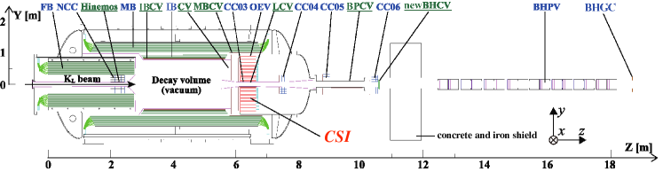
Figure 1 shows a cross-sectional view of the KOTO detector, where the coordinate origin is defined at the entrance of the detector. The CSI is located at , the downstream end of the decay volume. It consists of 2716 undoped CsI crystals, covering a circular area with a radius of cm and with a square hole for the beam to pass, as shown in Fig. 2. The CSI has two different sizes of crystals. Crystals with a size of are located in the central square region, and others with a size of are situated in the outer area. The small crystals are viewed by inch Hamamatsu R5364 PMTs, while the large crystals are viewed by inch Hamamatsu R5330 PMTs. The analog pulses from each PMT are digitized and recorded using custom-made 14-bit 125-MHz ADC modules [7]. For each event, 64 samples of voltages are recorded every 8 ns. In order to achieve a better timing resolution of the pulse, the analog pulse signal is reformed before digitization using a 10-pole Bessel filter. This Bessel filter is used to widen and transform the PMT pulse into a Gaussian shape to increase the number of sampling points in the pulse rising edge. The 14-bit dynamic range of the ADC covers energy deposits from sub-MeV to 2 GeV, with an energy deposit of 1 MeV resulting in a pulse height of 8-10 ADC counts. Further details on the CSI can be found in Ref. [5].
3 Cluster shape discrimination
3.1 Cluster shapes and data set
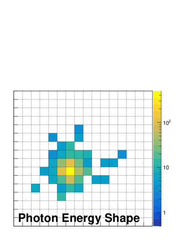
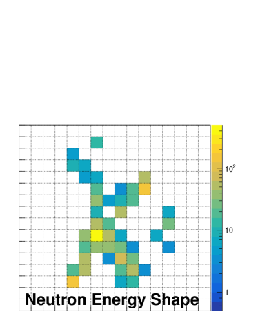
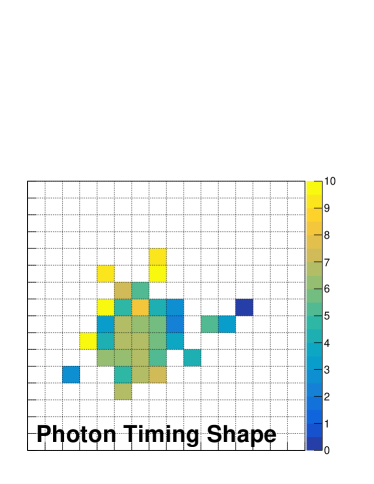
Cluster shape discrimination (CSD) is a method to distinguish photons from neutrons, based on their different characteristics in the cluster shapes. These differences arose from the interaction processes between electromagnetic interactions from photons and hadronic interactions from neutrons. For a pulse in a crystal, the energy was calculated by integrating ADC values of the digitized waveform, and the pulse timing was defined as the time of the waveform crossing half of its peak height. These measurements of energy and timing from each crystal in the CSI grid formed the cluster’s energy and timing distributions (shapes), which can be considered as images of particle interactions in the CSI. Figure 3 shows an illustration of the energy and timing shapes of photon and neutron clusters. Typically, photon clusters produced through electromagnetic interactions were more circular and symmetric in shapes. In general, the crystals closer to the incident point tend to have higher deposited energy due to the short radiation length of CSI. If photons have finite incident angles, crystals viewing the tail of the shower tend to have earlier timing, as they have energy deposits deeper in the crystal (closer to the PMT). On the other hand, neutron clusters produced through hadronic interactions had more asymmetrical energy and timing shapes.

In the CSD study, to optimize the CSD for selecting photons with the energy and angle spectrums from the decays, the photon samples were obtained from Monte Carlo (MC) events, generated using Geant4 simulations. To reflect actual beam activities and electronic noise, the MC events were overlaid with accidental data collected during data-taking. The photon samples were first selected by requiring two coincident clusters in the CSI and no in-time hits in other detector components. The decay vertex () and transverse momentum () of were then reconstructed by assuming the decay point to lie along the beam axis and the two clusters to have the invariant mass of . The events were selected by requiring the to be within the fiducial decay region of – mm. Additionally, the was required to be in the range of – MeV/, to account for the missing momentum carried by two neutrinos.
Neutron samples were obtained from special neutron data-taking runs conducted in 2016–2018. During these runs, an aluminum plate was placed at the detector entrance to scatter neutrons in the beam and enhance halo neutron events. The neutron data was collected by requiring two coincident clusters in the CSI and no hits in the major veto detectors. This sample was dominated by the events with a single neutron particle scattering within the CSI and producing two clusters. The neutron events were processed through the same reconstruction and selection procedures for the event candidates.
3.2 CNN and its network architecture
In the CSD study, a CNN was employed to differentiate between photon and neutron clusters based on their energy and timing shapes. The CNN is a popular deep-learning architecture used for image classification tasks. The input layer of the network consisted of the images of photon and neutron clusters, which were then processed through ten hidden layers, including four convolutional and six dense layers, as illustrated in Fig. 4.
The convolutional layers scanned each block of image pixels to identify local features of the cluster’s energy and timing images using 32 filters. Each filter was a tensor of weights and an offset bias. The output of the fourth convolutional layer, along with the incident particle’s energy () and direction (, ) as additional inputs, were processed by six dense layers. The dense layers were fully connected between two adjacent layers with 2048 neurons each to learn a non-linear function to produce the final output.
During network training, the neuron weights were calculated through the minimization of binary cross-entropy [9], which served as the loss function. This loss function provides an indication of the network model’s performance based on the deviations between the value predicted by the model and the actual true value. To prevent overtraining, the common L2 regularization [10] and dropout [11] techniques were applied to the network model. The L2 regularization, with a hyperparameter of , added a penalty term to the loss function at every layer of the model, making the neuron weights less sensitive to the training data. A dropout layer with the dropout rate of was inserted between dense layers. During the training, the dropout layer randomly deactivated of the neurons, promoting the network to learn multiple representations of the data. These hyperparameters were fine-tuned to ensure the model’s results were consistent between training and test samples. Finally, the output layer produced a probability distribution as the CSD score, with values closer to 1 indicating photon-like and values closer to 0 indicating neutron-like.
3.3 Training details
The input cluster images were generated from the cluster shape displayed in the CSI grid. Each pixel in the cluster image contained the energy and timing measured by the corresponding CsI crystal. There were three categories of cluster images: the clusters with small crystals only (Type-I), the clusters with large crystal only (Type-II), and the clusters with both types of crystals (Type-III). In each category, an equal number of photon and neutron images were used for the network training and were divided into three separate sets: training, validation, and test data. The training set was used for the network to learn and adjust the weights and biases of the model. The validation set was used to evaluate the model’s performance during the training process. The test set was used as a final evaluation of the performance of trained model. The ratio of data in the three sets was .
The size of the cluster images in Type-I and Type-II categories were and pixels, respectively. The Type-III cluster was treated like a Type-I cluster by dividing each large crystal into four small crystals, each containing of the energy. However, an additional layer was added to each pixel in the Type-III cluster image to indicate the crystal type. To achieve optimal performance, the CNN was trained separately on each of these three cluster categories.
The network was provided with additional inputs: the incident particle’s direction in spherical coordinates with the origin set at the reconstructed . Here, is the azimuthal angle of the cluster in the CSI surface plane, and is the incident angle of the particle to the CSI surface, with pointing to the beam axis direction. To simplify the input images and account for the eight-fold symmetrical layout of the CSI, the cluster images were mirrored and folded into the range of , as shown in Fig. 2. To allow the network to recognize cluster patterns from different directions, the cluster images in the training and validation sets were duplicated by transposing the cluster image pixels with . Moreover, each neutron cluster image in the training and validation samples was duplicated by randomly assigning its supplied input of incident angle . This data augmentation technique enabled the network to identify neutron clusters from a more generalized perspective, regardless of the reconstructed .
3.4 Training results
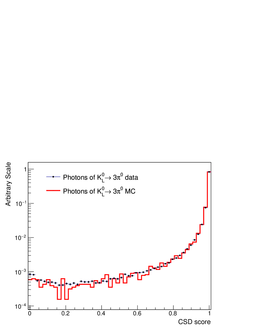
As mentioned in Section 3.2, the training of the CSD network was optimized to prevent overfitting. Our results indicated that the CSD performed consistently on the training, validation, and test sets, with slightly better performance on the test set. This was due to the fact that the data augmentation was only applied to the training and validation samples. The consistency between the data and MC simulations was verified by using the photon clusters from the events. The results showed that the CSD score of the data can be accurately reproduced by the MC simulations, as shown in Fig. 5. This indicates that the CSD method is reliable in distinguishing between photon and neutron clusters in actual data.
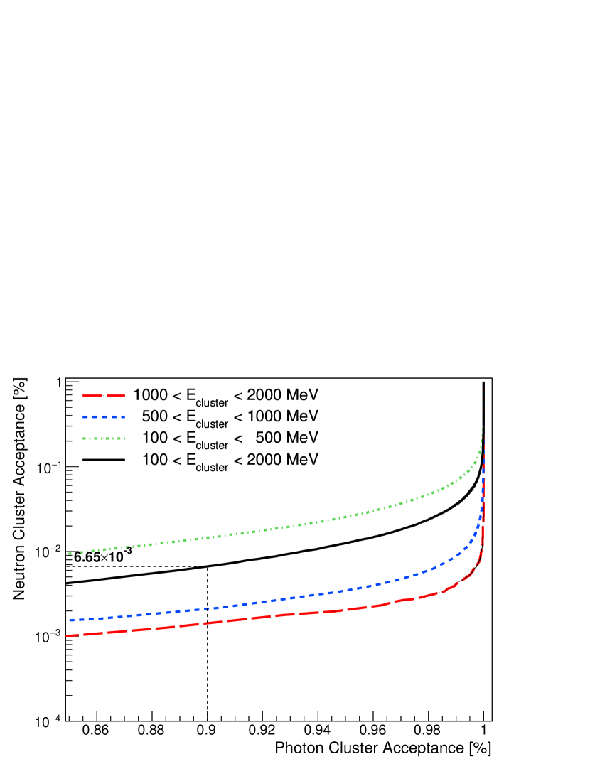
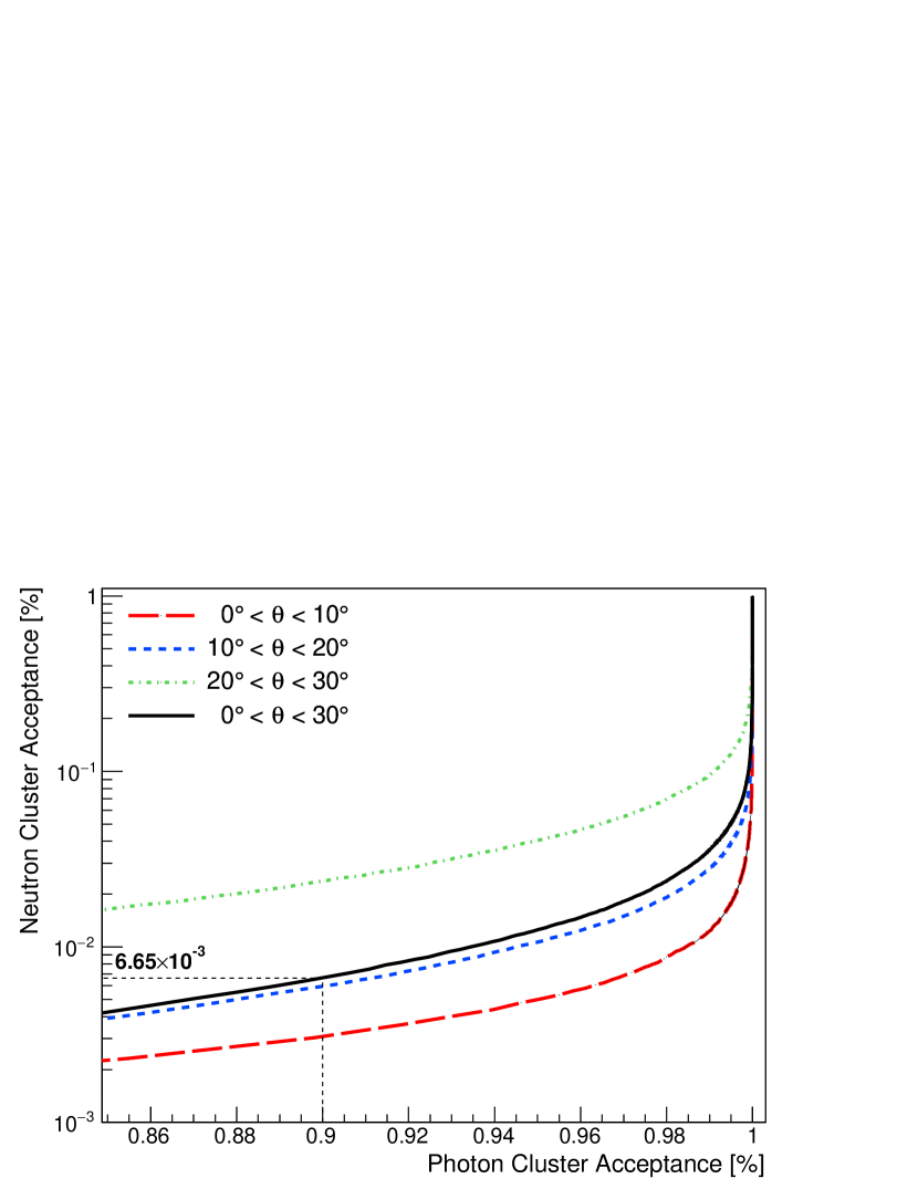
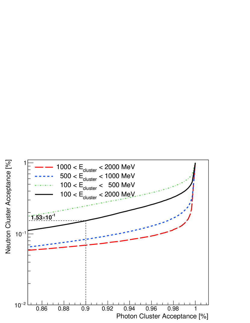
The performance of the CSD algorithm is presented by the acceptance of photon clusters in comparison to the acceptance of neutron clusters at various thresholds on the CSD score, as shown in Fig. 6. In general, the CSD had a higher discriminating power for higher energy clusters as larger cluster images contained more information on the cluster pattern features. After imposing veto and kinematic selection criteria for the events, the average energies of clusters from the neutron data samples and MC events were found to be similar, around 550 MeV. The results based on neutron data and MC events showed that the CSD algorithm effectively suppressed neutron clusters by a factor of , while maintaining a acceptance for photon clusters.
4 Pulse shape discrimination
4.1 Pulse shapes and data set
The pulse shape discrimination (PSD) is a method to distinguish between photon and neutron particles, based on their distinctive pulse shapes in the CSI. Neutron-induced pulses through hadronic interactions have a longer tail compared to those produced by photons through electromagnetic interactions, as shown in Fig. 7.
The intrinsic differences in the detector response between photon and neutron interactions were studied using photon and neutron samples in data. Photon samples were obtained from the data with six coincident clusters in the CSI and no in-time hits in major veto detectors. This sample was primarily dominated by events. For the neutron samples, the same data set described in Section 3.1 was used.
4.2 Discrimination method and results
In this study, the Discrete Fourier Transformation (DFT) was used to extract the differences between the neutron and photon pulses in the frequency domain. For a given CSI pulse, the DFT was applied to the ADC values of samples: , where is the ADC values of the sample. The first sample was chosen to align with the ADC values of the pulse peak. The DFT transformed into a sequence of 28 complex numbers () using the equation defined as:
| (1) |
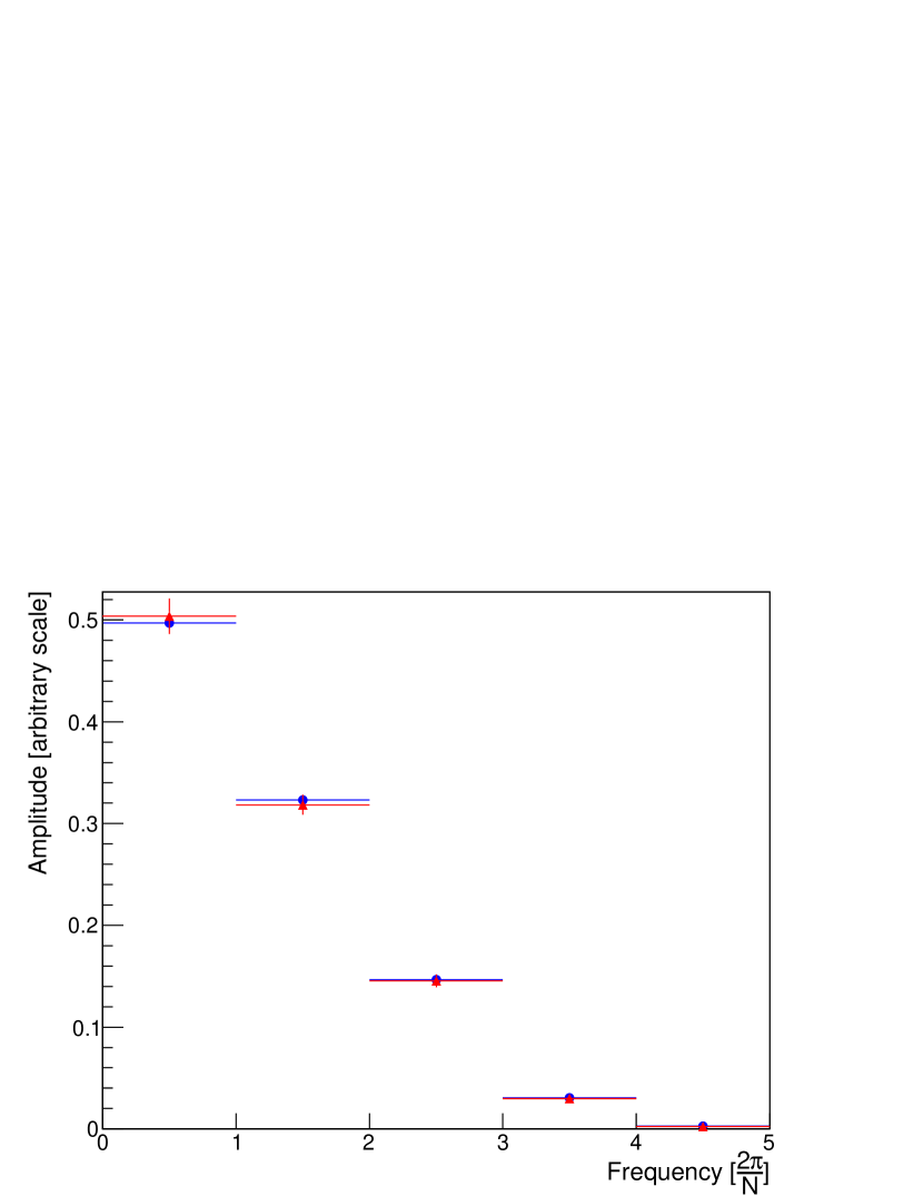
where the complex number encloses both amplitude and phase information for the complex sinusoid at the frequency of . The tail of the CSI pulse was represented by the amplitude () of the lower frequency sinusoids. In this analysis, the amplitudes of the lowest five frequency sinusoids, , were used to create templates for photons and neutrons, as shown in Fig. 8. To account for the pulse shape variations among crystals and energies, templates were created for each CsI crystal and for 20 bins in between . Each template includes five sets of , where and are the average and the standard deviation of , respectively.
To determine whether a given cluster is more photon-like or neutron-like, the likelihood of being either case was first calculated for each crystal contained in the cluster, which was defined as
| (2) |
where is the Fourier amplitudes of a crystal in the cluster, and are the templates of the photon or neutron Fourier amplitudes of that crystal. The likelihood of the cluster for being photon-like () or neutron-like () was then calculated by multiplying the likelihood of each crystal in the cluster as
| (3) |
where is the total number of crystals in the cluster.
With the photon and neutron likelihood values of a given cluster, the final likelihood ratio , or PSD score, was calculated as
| (4) |
The value of is between 0 and 1, with closer to 1 being photon-like and closer to 0 being neutron-like.
The performance of PSD is presented as the acceptance of photon clusters versus the acceptance of neutron clusters for different discrimination thresholds on the PSD score, as shown in Fig. 9. The results indicate that the PSD is more effective in discriminating high-energy clusters. To evaluate the realistic performance in differentiating between neutron clusters and photon clusters in the analysis, the energy spectrum of photon clusters in the data events was weighted to match that of clusters from MC events. It was evaluated that the PSD suppressed neutron clusters by a factor of while maintaining a acceptance for photon clusters from the events. In comparison to the method described in [6], this result with the DFT technique performed approximately twice as effective in suppressing neutron clusters.
5 Combined performance of CSD and PSD
The combined effectiveness of the CSD and PSD in suppressing neutron background events in the analysis was evaluated using an event-weighted method. This approach first calculated the survival probability () of individual neutron clusters under the combined rejections of the CSD and PSD. To take into account the energy () and incident angle () dependence of the CSD and PSD effectiveness, was derived as a function of and based on a large sample of neutron clusters. was then used to assign event weights to neutron events subjected to the CSD and PSD rejections. For a neutron event with two clusters, the event’s survival probability was calculated as the product of the individual cluster’s values: . To estimate the remaining neutron events in a certain region after the CSD and PSD rejections, the event-weighted method simply summed the survival probability of all events in that region, which gives
| (5) |
where counts the number of events in that region before the CSD and PSD rejections, and the was the estimated number of neutron events that may remain after the CSD and PSD rejections.
In this study, the neutron events in the Wide Signal Box (WSB) region were used for evaluating the effectiveness of the CSD and PSD in suppressing neutron background events. The WSB region was defined as mm and MeV/, as indicated in Fig. 10.

After imposing the event selection criteria without CSD and PSD to the neutron data, there were 5973 neutron events () in the WSB region. Based on these events, the estimated () and observed () number of neutron events, and the efficiency () after further imposing the CSD and PSD rejections with different thresholds are summarized in Table 1. With loose thresholds on the CSD and PSD scores, the results indicate that the number of observed neutron events () could be accurately predicted by , demonstrating the reliability of the event-weighted method. In the analysis of 2016–2018 data, the thresholds on the CSD and PSD scores were set at 0.985 and 0.5, respectively. Under these thresholds, the event-weighted method predicted remaining neutron events in the WSB region, while no events were actually observed. The acceptance of neutron events against the CSD and PSD rejections () was then calculated to be
which corresponds to a suppression factor of on the neutron background events. The efficiency of detecting under the same thresholds was determined to be .
| CSDThres | PSDThres | () | ||
|---|---|---|---|---|
| - | - | 5973 | - | |
| 0.0001 | 0.0001 | 528 | ||
| 0.0005 | 0.0005 | 161 | ||
| 0.001 | 0.001 | 105 | ||
| 0.005 | 0.005 | 34 | ||
| 0.01 | 0.01 | 22 | ||
| 0.05 | 0.05 | 5 | ||
| 0.1 | 0.1 | 4 | ||
| 0.5 | 0 | |||
| 0 |
6 Conclusion
We developed two analysis techniques to distinguish between photon and neutron events in the undoped CsI calorimeter of KOTO. These methods were based on the distinct characteristics in their cluster shapes displayed on the CSI grid and pulse shapes in each CsI crystal. We employed a convolutional neural network to classify the cluster shapes and Fourier frequency analysis to differentiate between the waveform shapes. The performance of discrimination was estimated through an event-weight method. As a result, we suppressed the neutron background events by a factor of , while maintaining the acceptance of at .
Acknowledgement
We would like to express our gratitude to all members of the J-PARC Accelerator and Hadron Experimental Facility groups for their support. We also thank the KEK Computing Research Center for KEKCC, the National Institute of Information for SINET4, and the University of Chicago Computational Institute for the GPU farm. This material is based upon work supported by the Ministry of Education, Culture, Sports, Science, and Technology (MEXT) of Japan and the Japan Society for the Promotion of Science (JSPS) under KAKENHI Grant Number JP16H06343 and through the Japan-U.S. Cooperative Research Program in High Energy Physics; the U.S. Department of Energy, Office of Science, Office of High Energy Physics, under Awards No. DE-SC0009798; the National Science and Technology Council (NSTC) and Ministry of Education (MOE) in Taiwan, under Grants No. NSTC-111-2112-M-002-036, NSTC-110-2112-M-002-020, MOE-111L894805, and MOE-111L104079 through National Taiwan University. We would also like to thank K. Kotera for the critical reading and suggestions for this article.
References
- [1] A. J. Buras, D. Buttazzo, J. Girrbach-Noe, and R. Knegjens, and in the Standard Model: status and perspectives, Journal of High Energy Physics, 11 (2015) 033.
- [2] J. K. Ahn et al. (KOTO Collaboration), Search for and Decays at the J-PARC KOTO Experiment, Physical Review Letters, 122 (2019) 021802.
- [3] J. K. Ahn et al. (KOTO Collaboration), Study of the Decay at the J-PARC KOTO Experiment, Physical Review Letters, 126 (2021) 121801.
- [4] T. Shimogawa et al., Design of the neutral beamline for the KOTO experiment, Nuclear Instruments and Methods in Physics Research Section A: Accelerators, Spectrometers, Detectors and Associated Equipment, 623 (2010) 585-587.
- [5] K. Sato et al., CsI calorimeter for the J-PARC KOTO experiment, Nuclear Instruments and Methods in Physics Research Section A: Accelerators, Spectrometers, Detectors and Associated Equipment, 982 (2020) 164527.
- [6] Y. Sugiyama et al., Pulse shape discrimination of photons and neutrons in the energy range of - GeV with the KOTO un-doped CsI calorimeter, Nuclear Instruments and Methods in Physics Research Section A: Accelerators, Spectrometers, Detectors and Associated Equipment, 987 (2021) 164825.
- [7] M. Bogdan et al., Custom 14-Bit, 125MHz ADC/Data Processing Module for the KL Experiment at J-Parc, in: 2007 IEEE Nuclear Science Symposium Conference Record, Vol. 1, IEEE, 2007, pp. 133–134. doi:10.1109/NSSMIC.2007.4436302.
- [8] K. T. O’Shea et al., An Introduction to Convolutional Neural Networks, eprint arXiv:1511.08458.
- [9] I. J. Goodfellow et al., Deep Learning, MIT Press, (2016).
- [10] A. Y. Ng, Feature selection, l1 vs. l2 regularization, and rotational invariance, in proceedings of the Twenty-first International Conference on Machine Learning, New York, NY, U.S.A., (2004) 78.
- [11] N. Srivastava et al., Dropout: A Simple Way to Prevent Neural Networks from Overfitting, Journal of Machine Learning Research, 15 (2014) 1929.