Genetic Composition of Supercritical Branching Populations under Power Law Mutation Rates

Abstract

We aim at understanding the evolution of the genetic composition of cancer cell populations. To this aim, we consider a branching individual based model representing a cell population where cells divide, die and mutate along the edges of a finite directed graph $(V,E)$. The process starts with only one cell of trait $0$. Following typical parameter values in cancer cell populations we study the model under large population and power law mutation rates limit, in the sense that the mutation probabilities are parameterized by negative powers of $n$ and the typical sizes of the population of interest are positive powers of $n$. Under non-increasing growth rate condition, we describe the time evolution of the first-order asymptotics of the size of each subpopulation on the $log(n)$ time scale, as well as in the random time scale at which the initial population, resp. the total population, reaches the size $n^{t}$. In particular, such results allow for the perfect characterization of evolutionary pathways. Without imposing any conditions on the growth rates, we describe the time evolution of the order of magnitude of each subpopulation, whose asymptotic limits are positive non-decreasing piecewise linear continuous functions.

Keywords: cancer evolution, multitype branching processes, finite graph, long time behavior, power law mutation rates, population genetics.
MSC2020 subject classifications: 60J80, 60J27, 60F99, 92D15, 92D25.

1 Introduction and presentation of the model

Consider a population of cells characterized by a phenotypic trait, where the trait space $V$ is finite. For all $v\in V$ denote by $(Z_{v}(t))_{t\in\mathbb{R}^{+}}$ the number of cells of trait $v$ at time $t$ in the population, and $\left(\mathcal{Z}(t):=\left(Z_{v}(t)\right)_{v\in V}\right)_{t\in\mathbb{R}^{+}}$ the global process. Assume that $0\in V$ and

$$\forall v\in V,Z_{v}(0)=\mathbbm{1}_{\{v=0\}},\text{ almost surely.}$$ (1.1)

Cells with trait $0$ are called wild-type cells, and all cells with trait $v\in V\backslash\{0\}$ are called mutant cells. The population dynamics will follow a continuous time branching process on $\mathbb{N}_{0}^{V}$. More precisely cells divide to give birth to two daughter cells and die with rates depending only on their phenotypic trait. The birth, death and growth rate functions are respectively

$$\alpha:V\longrightarrow\mathbb{R}^{+},\beta:V\longrightarrow\mathbb{R}^{+}\text{ and }\lambda:=\alpha-\beta.$$ (1.2)

During a division event of a cell of trait $v\in V$, independent mutations over the two daughter cells are considered. Mutation landscape across traits is encoded via a graph structure $(V,E)$ on the trait space. $E\subset\{(v,u),\forall v,u\in V^{2}\}$ is a set of ordered pairs over $V$ satisfying for all $v\in V$, $(v,v)\cap E=\emptyset$, and such that for all trait $v$ it exists a path from $0$ to $v$. In other words, $(V,E)$ is a finite oriented graph without self-loop for which each vertex is on the connected component of trait $0$. Mutation from a trait $v$ to a trait $u$ is possible if and only if $(v,u)\in E$. Let $\mu:E\longrightarrow[0,1]$ be a mutation kernel satisfying

$$\forall v\in V,\overline{\mu}(v):=\sum_{u\in V:(v,u)\in E}\mu(v,u)\leq 1.$$ (1.3)

A daughter cell mutates from trait $v$ to trait $u$ with probability $\mu(v,u)$, meaning that $\overline{\mu}(v)$ is its total mutation probability. Notice that backward mutations are contained in this model.

Finally the exact transition rates from a state $z=(z_{v})_{v\in V}\in\mathbb{N}_{0}^{V}$ of the process $\mathcal{Z}$ are

$$z\mapsto\left\{\begin{array}[]{l l l}&z-\delta_{v},\mbox{ at rate }z_{v}\beta(v),\\ &z-\delta_{v}+\delta_{u}+\delta_{w},\mbox{ at rate }2z_{v}\alpha(v)\mu(v,u)\mu(v,w)\mathbbm{1}_{\{(v,u)\in E\}}\mathbbm{1}_{\{(v,w)\in E\}}\mathbbm{1}_{\{u\neq w\}},\\ &z-\delta_{v}+2\delta_{u},\mbox{ at rate }z_{v}\alpha(v)\mu(v,u)^{2}\mathbbm{1}_{\{(v,u)\in E\}},\\ &z+\delta_{v},\mbox{ at rate }z_{v}\alpha(v)\left(1-\overline{\mu}(v)\right)^{2}+2\underset{u\in V:(u,v)\in E}{\sum}z_{u}\alpha(u)\mu(u,v)\left(1-\overline{\mu}(u)\right),\end{array}\right.$$ (1.8)

where $\forall v\in V,\delta_{v}=\left(\mathbbm{1}_{\{u=v\}}\right)_{u\in V}$. Through the paper, the growth rate of the wild-type subpopulation is assumed to be strictly positive $\lambda(0)>0$, otherwise the wild-type subpopulation won’t survive almost surely.

The biological motivation of this model is to capture the dynamics over time of the genetic composition of a population of cells during carcinogenesis. Tumors are detected when they reach a size of a large amount of cells, typically $10^{9}$ cells. The mutation rates per base pair per cell division is generally estimated to be of order $10^{-9}$, see [1, 2]. Then it naturally invites to consider the framework of large population and power law mutation rates limit. A parameter $n\in\mathbb{N}$ is used to quantify both the decrease of the mutation probabilities, as negative powers of $n$, and also the typical size of the population, depending on $n$ as positive power of $n$, at which we are interested in understanding the genetic composition. The aim is to obtain asymptotic results on the sizes of all the mutant subpopulations when $n$ goes to infinity. It is a classical stochastic regime studied in particular in [3, 4, 5, 6, 7, 8, 9, 10, 11, 12, 13, 14]. Such regime is referred in [5, 7] as the large population rare mutations limit, but we decided to take the precision of power law mutation rates in order to distinguish such regime with the classical rare mutation limit where the mutation probabilities $\mu^{(n)}$ scale typically as $e^{-Cn}\ll\mu^{(n)}\ll\frac{1}{n\log(n)}$. Indeed with the large population power law mutation rates limit, the mutation probabilities can be of a higher order than with the rare mutation limit if for instance $\mu^{(n)}\propto n^{-\alpha}$ with $\alpha\in(0,1]$.

To be more precise, let $L:=\{\ell(v,u)\in\mathbb{R}_{+}^{*},\forall(v,u)\in E\}$ be a set of strictly positive labels on the edges of the graph. Introduce a sequence of models $\left(\mathcal{Z}^{(n)}\right)_{n\in\mathbb{N}}$, where for each $n\in\mathbb{N}$, $\mathcal{Z}^{(n)}$ corresponds to the process described above with the mutation kernel $\mu^{(n)}:E\longrightarrow[0,1]$ satisfying

$$\forall(v,u)\in E,n^{\ell(v,u)}\mu^{(n)}(v,u)\underset{n\to\infty}{\longrightarrow}\mu(v,u)\in\mathbb{R}^{+}.$$ (1.9)

For all $t\in\mathbb{R}_{+}^{*}$, the stopping times corresponding to the first time that the wild-type subpopulation $Z_{0}^{(n)}$, respectively the total population $Z^{(n)}_{tot}:=\sum_{v\in V}Z_{v}^{(n)}$, reaches the level $n^{t}$, are defined as

$$\eta_{t}^{(n)}:=\inf\left\{u\in\mathbb{R}^{+}:Z_{0}^{(n)}(u)\geq n^{t}\right\}\text{ and }\sigma_{t}^{(n)}:=\inf\left\{u\in\mathbb{R}^{+}:Z^{(n)}_{tot}(u)\geq n^{t}\right\}.$$ (1.10)

Two different biological interpretations in different settings can be made in order to motivate both of them. For instance, when considering metastasis the wild-type subpopulation $Z_{0}^{(n)}$ may represent the primary tumor, and the mutant subpopulations $Z_{v}^{(n)},$ for all $v\in V\backslash\{0\}$, may correspond to secondary tumors. As it is size and not age of a tumor that clinicians have access to, it is biologically relevant to estimate the genetic composition of the secondary tumors when the primary one has a given size. This is mathematically encoded in looking at the first-order asymptotics of $Z_{v}^{(n)}\big{(}\eta_{t}^{(n)}\big{)}$ for all $v\in V\backslash\{0\}$. Another biological setting is when the total population $Z^{(n)}_{tot}$ represents one tumor. It is appropriate to obtain theoretical results about the size of the mutant subpopulations $Z_{v}^{(n)}$ for all $v\in V\backslash\{0\}$ when the tumor has reached a given size. It corresponds exactly to look at the first-order asymptotics of $Z_{v}^{(n)}\big{(}\sigma_{t}^{(n)}\big{)}$. Every time that results can be stated either with $\eta_{t}^{(n)}$ or $\sigma_{t}^{(n)}$, the following notation will be used

$$\rho_{t}^{(n)}:=\eta_{t}^{(n)}\text{ or }\sigma_{t}^{(n)}.$$ (1.11)

In the present work the population of cells will be studied in different time-scales: the random time-scale

$$\Big{(}\rho_{t}^{(n)}+s\Big{)}_{(t,s)\in\mathbb{R}^{+}\times\mathbb{R}};$$ (1.12)

and the following deterministic approximation

$$\Big{(}\mathfrak{t}^{(n)}_{t}+s\Big{)}_{(t,s)\in\mathbb{R}^{+}\times\mathbb{R}},\text{ with }\mathfrak{t}^{(n)}_{t}:=t\frac{\log(n)}{\lambda(0)}.$$ (1.13)

Intuitively, the lineage of wild-type cells generated from the initial cell is the first subpopulation that will allow to create mutations. Then understanding its growth gives the natural time scale to consider for seeing mutations. Its birth and death rates are $\alpha(0)\left(1-\overline{\mu}^{(n)}(0)\right)^{2}$ and $\beta(0)+\alpha(0)\left(\overline{\mu}^{(n)}(0)\right)^{2}$ respectively. Because of the power law mutation rates regime of Equation (1.9) they are converging to $\alpha(0)$ and $\beta(0)$ when $n$ grows to $\infty$. Meaning that this lineage should behave asymptotically as a birth and death process with rates $\alpha(0)$ and $\beta(0)$. Indeed such a result emerges on the natural martingale associated to a birth and death process, see Lemma 3.1. In particular the growth rate of this lineage is close to $\lambda(0)$ thus this population reaches a size of order $n^{t}$ approximately at the deterministic time $\mathfrak{t}_{t}^{(n)}$, see Lemma 3.2.

For any finite oriented labeled graph $(V,E,L)$ under the following non-increasing growth rate condition

$$\forall v\in V,\lambda(v)\leq\lambda(0),$$ (1.14)

the first-order asymptotics of the sizes of all the mutant subpopulations $Z_{v}^{(n)}$ are obtained both in random and deterministic time scales (1.12) and (1.13), see Theorem 2.7. Assumption (1.14) can be biologically motivated. Historically tumor dynamics has been seen under the prism of clonal expansion of selective mutations, i.e. $\lambda(v)>\lambda(0)$. Nevertheless the paradigm of neutral evolution of cancer has been recently considered, see [15, 16, 17, 18, 19], meaning that the selective mutations are already present in the initial cell and that the occurring mutations are neutral ones (i.e. $\lambda(v)=\lambda(0)$). With Assumption (1.14) deleterious mutations (i.e. $\lambda(v)<\lambda(0)$) are also considered. This paradigm has been introduced because the genetic heterogeneity inside a tumor could be explained only considering neutral mutations. Various statistical methods are developed to infer the evolutionary history of tumors, including test of neutral evolution, see [20, 21, 22] for details about that.

Without any assumption on the growth rate function $\lambda$, the study is made on the deterministic time scale of Equation (1.13). As in [3, 6, 8, 9, 10, 11, 12, 14] the asymptotic behaviors are obtained on the following stochastic exponent processes

$$\forall v\in V,X_{v}^{(n)}(t):=\frac{\log^{+}\big{(}Z_{v}^{(n)}\big{(}\mathfrak{t}^{(n)}_{t}\big{)}\big{)}}{\log(n)/\lambda(0)}.$$ (1.15)

The results are presented in Theorem 2.9. It is the exponent as a power of $n$ that is tracked for any subpopulation, whereas Theorem 2.7 gives directly the size order on $n$, this is a refined result. Up to our knowledge, it is the first model considering the power law mutation rates regime (1.9) capturing this level of refinement on the asymptotic behaviors. Two new significant results emerge.

First it shows the remarkable result that under Assumption (1.14) the randomness on the first-order asymptotics of the size of any mutant subpopulation is fully given by the stochasticity of only one random variable $W$ -encoding the randomness on the long time for the lineage of wild-type cells issued from the initial cell. More precisely the stochasticity for any mutant subpopulation is fully driven, at least at the first-order asymptotics, by the randomness on the growth of the wild-type subpopulation and not from the dynamics of any lineage of a mutant cell, as well as the stochastic processes generating mutations.

Second it characterizes exactly whether a mutational path on the graph structure of the trait space asymptotically contributes to the growth of the mutant subpopulations. Whereas having asymptotic results on the stochastic exponents only allows to discriminate some paths and not to determine exactly whose paths are actually contributing to the asymptotic growth of the mutant subpopulations. More precisely, if the length of a path is defined as the sum of the labels of its edges, asymptotic results on the stochastic exponent gives that for all trait $v$, among the paths from $0$ to $v$ only those with the minimal length might contribute to the asymptotic growth of trait $v$. On the contrary, having results directly on the first-order asymptotics of the size of the mutant subpopulations allows to discriminate among those paths with the minimal length those which actually contribute to the dynamics of trait $v$. In particular among those paths with the minimal length only those with the maximal number of neutral mutations on their edges have an asymptotic impact on the growth of trait $v$. Indeed an additional multiplicative factor of order $\log(n)$ for each neutral mutation of a path is captured when looking at the first-order asymptotics and is obviously not captured with asymptotic results only on the stochastic exponents. Broadly speaking it says that among two paths with the same mutational burden (in the sense having the same length) only the one with the maximal number of neutral mutation will asymptotically contribute. Such theoretical result opens the door for developing new statistical methods to infer the underlying graph structure from data observation, i.e. to infer the evolutionary history of tumors, as well as designing new statistical estimators for biologically relevant parameters.

Moreover it is the first time that this power-law mutation rates limit is studied in the random time-scale of Equation (1.12) up to our knowledge. From the biological point of view it is more interesting to get results on such random time scale instead of the deterministic one. We obtain that the randomness on the first-order asymptotics of the size of any mutant subpopulation is fully given by the stochasticity on the survival of the lineage of wild-type cells issued from the initial cell.

In [5, 7] Cheek and Antal study a model that can be seen as an application of the model of the present work via a specific finite oriented labeled graph $(V,E,L)$. Among their results, they fully characterize in distribution the asymptotic sizes of all the mutant subpopulations around the random time at which the wild-type subpopulation reaches the typical size allowing mutations to occur. In their setting it corresponds to $\big{(}\eta_{1}^{(n)}+s\big{)}_{s\in\mathbb{R}}$. In particular they obtain that the asymptotic sizes of all the mutant subpopulations around this random time $\eta_{1}^{(n)}$ are finite almost surely, following generalised Luria-Delbrück distributions, see Theorem 5.1 in [7]. The initial Luria and Delbrück model has generated many subsequent works, see in particular [23, 24, 25, 26, 27, 28, 5, 7]. Two major features explain the latter result. The first one is that asymptotically only a finite number of mutant cells are generated from the wild-type subpopulation until time $\eta_{1}^{(n)}$, following a Poisson distribution. The second one is that all the lineages of the mutant cells generated from the wild-type subpopulation have only, up to time $\eta_{1}^{(n)}$, asymptotically a finite random time to grow, which is exponentially distributed. We extend their results to larger times, typically when the total mutation rate from the subpopulation of a trait $v$ to the subpopulation of a trait $u$ is growing as a positive power of $n$, instead of remaining finite.

In [3] Durrett and Mayberry study the exponentially growing Moran model. They consider the same mutation regime, their size of the total population is growing exponentially fast at a fixed rate, and new individuals in the population chose their trait via a selective frequency dependent process. In Theorem 2.9 a similar result is obtained for the case of a multitype branching population. In particular, for this setting the exponential speed of the total population (and of the dominant subpopulations) is evolving through time. More specifically, we show that the speed is a non-decreasing piecewise constant function going from $\lambda(0)$ to $\underset{v\in V}{\max}\lambda(v)$, and taking values only on the set $\left\{\lambda(v),\forall v\in V\right\}$.

In [5, 4, 6, 8, 9, 10, 11, 12, 14], the authors are considering the large population and power law mutation rates limit of Equation (1.9) in the special case where all different traits mutate with the same scaling of a fixed order of a negative power of $n$. Whereas in the present work the power law mutation rates are more general by allowing traits to mutate with different scalings, as in [7, 13].

As in [5, 7], compared to the different models in [3, 4, 8, 9, 10, 11, 13, 14], the initial population $\mathcal{Z}^{(n)}(0)$ is not assumed to have a macroscopic size. It introduces a supplementary randomness on how the wild-type subpopulation is stochastically growing to get a macroscopic size. But contrary to [5, 7], we do not condition on the survival of the wild-type subpopulation or on the stopping times of Equation (1.11) to be finite.

In [29] Nicholson and Antal study a similar model under a slightly less general non-increasing growth rate condition. More precisely, in their case all the growth rates of the mutant populations are strictly smaller than the growth rate of the wild-type population: $\forall v\in V\backslash\{0\},\lambda(v)<\lambda(0)$. But the main difference remains the mutation regime. In their case, only the last mutation is in the power law mutation rates regime, all other mutations have a fixed probability independent of $n$. In Theorem 2.7 the case where all mutations are in the power law mutation rates regime is analysed. Also Nicholson and Antal are interested in obtaining the distribution of the first time that a mutant subpopulation gets a mutant cell. Whereas in the present work the first-order asymptotics of the sizes of the mutant subpopulations over time are studied.

In [30] Nicholson, Cheek and Antal study the case of a mono-directional graph where the time tends to infinity with fixed mutation probabilities. In particular they obtain the almost sure first-order asymptotics of the sizes of the different mutant subpopulations. Under the non-increasing growth rate condition, they are able to characterized the distribution of the random variables they obtained at the limit. Without any condition on the growth rates, they study the distribution of the random limit they obtained under the small mutation probabilities limit, using the hypothesis of an approximating model with less stochasticity. Notice that the mutation regime they study is not the large population power law mutation rates limit of Equation (1.9) as considered in the present work. Under the latter regime both the size of the population goes to infinity and the mutation probabilities to 0, through the parameter $n$.

In [31] Gunnarson, Leder and Zhang study a similar model as the one in the present work and are also interested in capturing the evolution over time of the genetic diversity of a population of cells, using in their case the well-known summary statistic called the site frequency spectrum (SFS). The main difference is the mutation regime because they are not considering the power law mutation rates limit. In their case the mutation probabilities are fixed. Also, they restrict the study to the neutral cancer evolution case. In particular, as in the present work, they capture the first-order asymptotics of the SFS at a fixed time and at the random time at which the population first reaches a certain size. Two noticeable similarities in the results are that the first-order asymptotics of the SFS converges to a random limit when evaluated at a fixed time and to a deterministic limit when evaluated at the stochastic previous time. One could argue that in the present work the correct convergence in the latter case is actually a stochastic limit. But the randomness is fully given by the survival of the initial lineage of cells of trait $0$, so conditioned on such an event at the end the limit is a deterministic one. In particular the results of Gunnarson, Leder and Zhang are all conditioned on nonextinction of the population.

In [13] Gamblin, Gandon, Blanquart and Lambert study a model of an exponentially growing asexual population that undergoes cyclic bottlenecks under the large population and power law mutation rates limit. Their trait space is composed of 4 subpopulations $00,10,01$ and $11$, where two paths of mutations are possible $00\mapsto 10\mapsto 11$ and $00\mapsto 01\mapsto 11$. They study the special case where one mutation ($10$) has a high-rate but is a weakly beneficial mutation whereas the other mutation ($01$) has a low-rate but is a strongly beneficial mutation. In particular they show the noticeable result that due to cyclic bottlenecks only a unique evolutionary path unfolds but modifying their intensity and period implies that all paths can be explored. Their work relies on a deterministic approximation of the wild-type subpopulation $00$ and some parts of the analysis of the behavior of the model is only obtained due to heuristics. The present work, and more specifically Theorem 2.9, because they are considering selective mutations, can be used and adapted to consider the case of cyclic bottlenecks in order to prove rigorously their results, in the specific trait space that they consider as well as on a general finite trait space.

The rest of the paper is organised as follows. In Section 2 the results and their biological interpretations are given. Sections 3 and 4 are dedicated to prove Theorem 2.7, which assumes Equation (1.14). In Section 3 the mathematical definition of the model is given for an infinite mono-directional graph as well as the proof in this particular case. The generalisation of the proof from an infinite mono-directional graph to a general finite graph is given in Section 4. In Section 5, Theorem 2.9 is proved adapting results from [3].

2 Main results and biological interpretation

In Subsection 2.1 the first-order asymptotics of the size of each mutant subpopulation in the time scales (1.12) and (1.13) are given under the non-increasing growth rate condition (1.14). In Subsection 2.2 the asymptotic result on the stochastic exponent of each mutant subpopulation is given without any assumption on the growth rate function $\lambda$. In each subsection, biological interpretations of the results are made.

2.1 First-order asymptotics of the mutant subpopulation sizes under non-increasing growth rate condition

In this subsection assume that $(V,E,L)$ satisfies the non-increasing growth rate graph condition of Equation (1.14).

Heuristics:

The next definitions, notations and results are first motivated using some heuristics for the simplest graph that one can think of, i.e. a wild-type and a mutant population where only mutations from wild-type to mutant cells are considered. More precisely $(V,E,L)=\left(\{0,1\},\{(0,1)\},\{\ell(0,1)\}\right)$ as in Figure 1.

Figure 1: Graphical representation of the two traits model without backward mutation

Under the power law mutation rates regime, the inner birth and death rate of the wild-type subpopulation, respectively $\alpha(0)\left(1-\mu^{(n)}(0,1)\right)^{2}$ and $\beta(0)+\alpha(0)\left(\mu^{(n)}(0,1)\right)^{2}$, are so close to $\alpha(0)$ and $\beta(0)$ respectively that its natural martingale asymptotically behaves as the one of a birth and death process with rates $\alpha(0)$ and $\beta(0)$ (Lemma 3.1). This fact allows to approximate the growth of the wild-type subpopulation as an exponential growth of parameter $\lambda(0)$. Then if it survives, at time $\mathfrak{t}^{(n)}_{t}$ (see (1.13)) its size is of order $\mathcal{O}\left(n^{t}\right)$ (Lemma 3.2). From this fact, one understands why it is necessary to wait for time $\mathfrak{t}^{(n)}_{\ell(0,1)}$ before seeing any mutation. Indeed, with a mutation probability which scales as $n^{-\ell(0,1)}$, the total mutation probability up to time $\mathfrak{t}^{(n)}_{t}$ scales as $\int_{0}^{t}n^{u}n^{-\ell(0,1)}d\big{(}u\frac{\log(n)}{\lambda(0)}\big{)}=\frac{n^{-\ell(0,1)}}{\lambda(0)}\left(n^{t}-1\right)$ which starts to be of order 1 for $t\geq\ell(0,1)$. This is made formal by D. Cheek and T. Antal in [5, 7] and an illustration can be found at Figure 2.

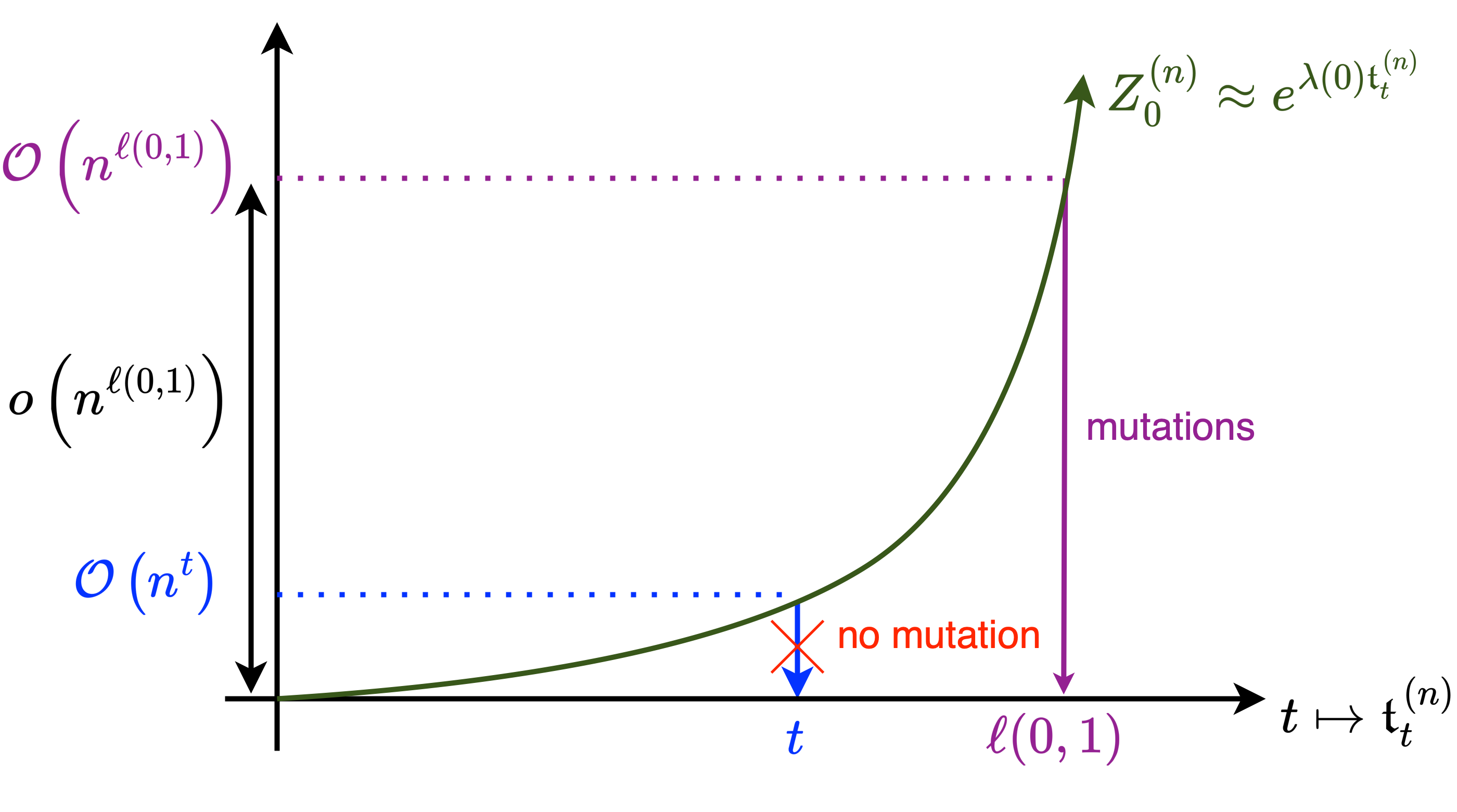
Figure 2: Heuristics for the first-occurrence time of mutant cells

It is also possible to get some heuristics for the size of the mutant subpopulation for time $\mathfrak{t}^{(n)}_{t},$ for $t\geq\ell(0,1)$. Let $\ell(0,1)\leq u\leq t$, the number of new mutations generated at time $\mathfrak{t}_{u}^{(n)}$ scales as $\exp\big{(}\lambda(0)(u-\ell(0,1))\frac{\log(n)}{\lambda(0)}\big{)}$. The remaining time for these new mutant cells to grow exponentially fast at rate $\lambda(1)$ until time $\mathfrak{t}_{t}^{(n)}$ is $\mathfrak{t}_{t-u}^{(n)}$. This implies that their lineages get at time $\mathfrak{t}_{t}^{(n)}$ a size of order

$$\mathcal{O}\Big{(}\exp\Big{(}\left[\lambda(1)t+(\lambda(0)-\lambda(1))u-\lambda(0)\ell(0,1)\right]\frac{\log(n)}{\lambda(0)}\Big{)}\Big{)}.$$ (2.1)

Then two scenari are possible:

• If $\lambda(1)<\lambda(0)$: Equation (2.1) is maximal for $u=t$ and equal to $n^{t-\ell(0,1)}$. This means that the dynamics of the mutant subpopulation is driven by the mutation from the wild-type subpopulation and not from its inner growth. More precisely its size order at time $\mathfrak{t}_{t}^{(n)}$ is fully given by the mutations generated at this time -and so is of order $n^{t-\ell(0,1)}$- and not from the lineages issued from mutations at strictly previous time. Biologically these mutations are called deleterious.

• If $\lambda(1)=\lambda(0)$: Equation (2.1) is independent of $u$ and equal to $\mathcal{O}\left(n^{t-\ell(0,1)}\right)$ for any $\ell(0,1)\leq u\leq t$. This means that these lineages have the same size order at time $\mathfrak{t}_{t}^{(n)}$ than any other lineage of mutant cells generated from mutational events at any other time between $\mathfrak{t}_{\ell(0,1)}^{(n)}$ and $\mathfrak{t}_{t}^{(n)}$. To put it differently, in the dynamics of the mutant subpopulation there is a balance between the contribution of mutations and its inner growth. This is a consequence of assuming $\lambda(1)=\lambda(0)$. These mutations are referred as neutral mutation, even if biologically speaking it would have exactly mean the more restrictive condition $\alpha(1)=\alpha(0)$ and $\beta(1)=\beta(0)$. Hence to capture the total size of the mutant subpopulation at time $\mathfrak{t}^{(n)}_{t}$, it remains to integrate all the lineages issued from mutational events over time $\mathfrak{t}_{u}^{(n)},$ for $\ell(0,1)\leq u\leq t$. It gives exactly the order $\mathcal{O}\left((t-\ell(0,1))\log(n)n^{t-\ell(0,1)}\right)$.

To sum up, for this simple graph, the mutant subpopulation scales after time $\mathfrak{t}_{\ell(0,1)}^{(n)}$ as

$$\mathcal{O}\Big{(}n^{t-\ell(0,1)}\left[\mathbbm{1}_{\{\lambda(0)>\lambda(1)\}}+\mathbbm{1}_{\{\lambda(0)=\lambda(1)\}}(t-\ell(0,1))\log(n)\right]\Big{)}.$$ (2.2)

Notice in particular that in any case, the mutant subpopulation has an exponential growth at rate $\lambda(0)$ after time $\mathfrak{t}^{(n)}_{\ell(0,1)}$, given by the factor $n^{t-\ell(0,1)}$. An illustration of this heuristic can be found in Figure 3.

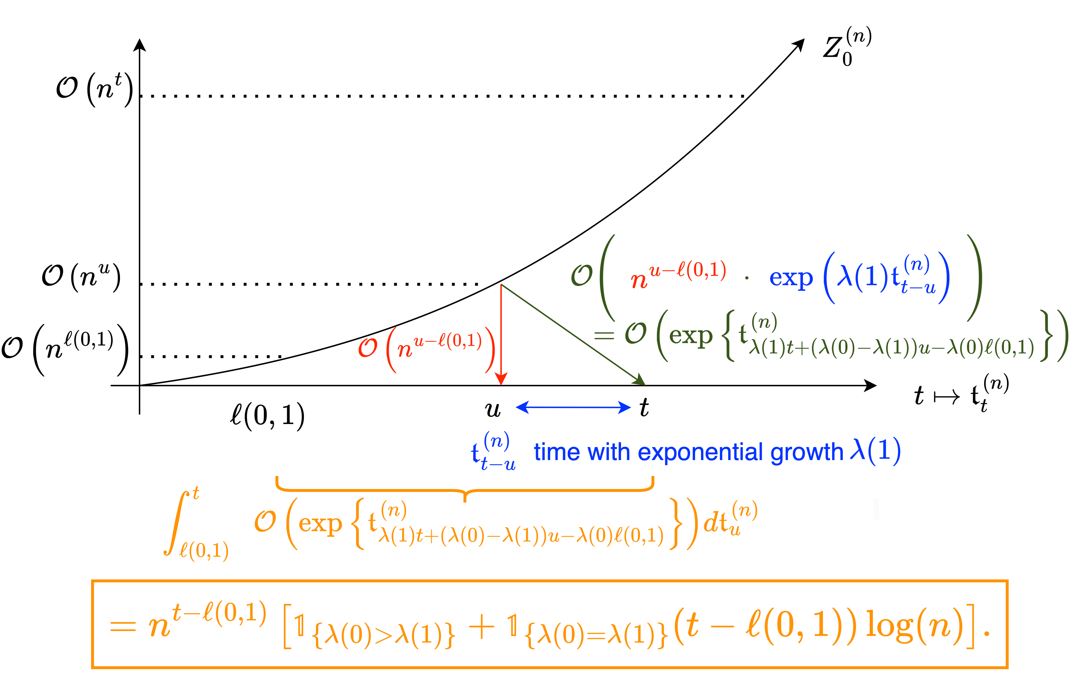
Figure 3: Heuristics for the size of the mutant subpopulation after time $\mathfrak{t}_{\ell(0,1)}^{(n)}$

These heuristics on this simple graph can be used as an elementary brick for getting heuristics on a general finite graph. Considering a vertex $v\in V\backslash\{0\}$, there are potentially many mutational paths from the initial vertex $0$ to $v$. Then it needs to be understood which ones are involved in the size order of the mutant subpopulation of trait $v$. Using both the previous heuristics on the first-occurrence time for mutations to be generated and that after this time the mutant subpopulation grows exponentially fast at rate $\lambda(0)$ as well as it gets a $\log(n)$ factor whether it is a neutral mutation, it seems natural to iteratively apply the reasoning to get heuristics on mutational paths. Thus given one path from $0$ to $v$, the time $u$ in the time scale $\mathfrak{t}^{(n)}_{u}$ to wait for seeing a cell of trait $v$ generated due to this specific path is the sum of the labels of the edges of this path, called the length of this path. Then, after this time, this subpopulation of cells of trait $v$ grows exponentially fast at rate $\lambda(0)$. Moreover, as seen in (2.2), for any neutral mutation on the path a supplementary multiplicative factor of order $\log(n)$ is captured on the size order. These two facts are summed up as after time the length of this path, this subpopulation grows exponentially fast at rate $\lambda(0)$ and has a multiplicative factor $\log(n)$ to the power the number of neutral mutations there are on this path. In particular three interesting facts for the total mutant subpopulation of trait $v$ are brought out. First it starts having cells after a time which is the minimum of the lengths over the paths from $0$ to $v$. Second, after this time only the paths whose lengths are equal to the latter minimum might contribute to the size order of the mutant cells of trait $v$. This is due to the fact that having a time delay create an exponential delay in the size order. This fact is asymptotically captured in Theorem 2.9. Thirdly, the supplementary multiplicative factor of order $\log(n)$ due to the neutral mutations implies that over the paths from $0$ to $v$ satisfying that their lengths are equal to the latter minimum, only those with the maximal number of neutral mutations are actually contributing to the size order of the mutant subpopulation of trait $v$. More specifically with a factor of $\log(n)$ at the power this maximal number of neutral mutations. This fact is asymptotically captured in Theorem 2.7. Moreover for any of these admissible paths, at each neutral mutation a supplementary time integral is obtained, as seen in (2.2). An illustration with an example is given in Figure 4.

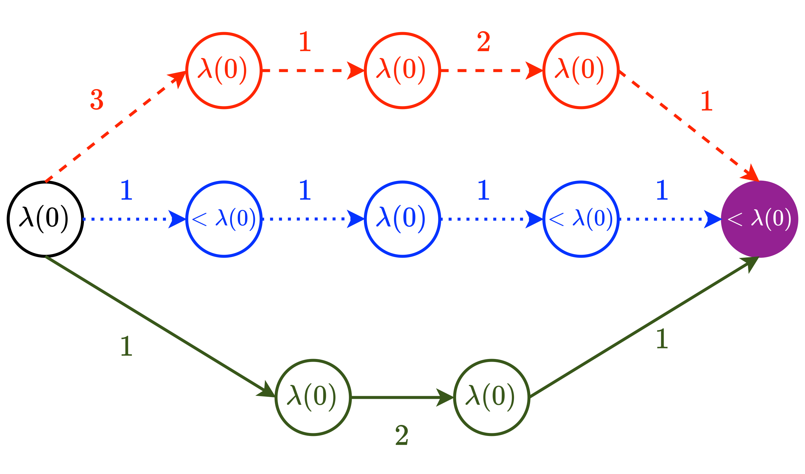
Figure 4: Heuristics for the contribution of paths in the size order of a mutant subpopulation: in this example the dashed red path has a length equal to 7 whereas the dotted blue and the plain green ones have a length equal to 4. Thus, only the two latter ones may contribute to the size order of the mutant, and so are sub-admissible paths. But the dotted blue path has only one neutral mutation compared to the plain green one which has two neutral mutations. Finally, only the plain green path will contribute to the size order of the purple mutant subpopulation. For $t\geq 4$, at time $\mathfrak{t}^{(n)}_{t}$ it will grow as $\log^{2}(n)e^{\lambda(0)\mathfrak{t}^{(n)}_{t-4}}$. Notice in particular that the dashed red path has the maximal number of neutral mutations equal to 3, but since it is not an sub-admissible path the multiplicative factor of $log(n)$ remains $2$ instead of $3$.

Notations:

Now the natural definitions issued from these heuristics are formally made before giving the results.

Definition 2.1 (Deleterious and neutral vertices).

A vertex $v\in V$ satisfying $\lambda(v)=\lambda(0)$, respectively $\lambda(v)<\lambda(0)$, is called a neutral, respectively deleterious, vertex.

Remark 2.2.

In the previous definition the neutral or deleterious denomination of a mutation originates from the comparison of its inner growth rate to the growth rate of the wild-type population. But one could imagine a mutation from a vertex $v$ to a vertex $u$ satisfying $\lambda(v)<\lambda(u)\leq\lambda(0)$. This mutation should theoretically be called selective, since $\lambda(u)>\lambda(v)$, but in the previous definition it is actually called neutral or deleterious (depending on the value of $\lambda(u)$ compared to $\lambda(0)$). This nomenclature emerges from the fact that under Assumption (1.14) any mutant subpopulation grows exponentially fast at rate $\lambda(0)$, as seen in the previous heuristics. Hence it legitimates the previous definition, assuming (1.14).

Definition 2.3 (Path on the graph).

$\gamma=(v(0),\cdots,v(k))$ is said to be the path on the graph $(V,E)$ linking $v(0)$ to $v(k)$ using the edges $(v(i),v(i+1))$ if for all $0\leq i\leq k,v(i)\in V\text{ and }\forall 0\leq i\leq k-1,(v(i),v(i+1))\in E$. For a path $\gamma=(v(0),v(1),\cdots v(k))$ on $(V,E,L)$ define

$$t(\gamma):=\sum_{i=0}^{k-1}\ell(v(i),v(i+1)),$$ (2.3)

$$\gamma_{neut}=\{v(i),1\leq i\leq k:\lambda(v(i))=\lambda(0)\},$$ (2.4)

$$\theta(\gamma):=|\gamma_{neut}|,$$ (2.5)

as respectively the sum of the labels of the edges of the path $\gamma$, the subset of vertices at the end of the edges of $\gamma$ that are neutral, and the cardinal of the previous subset. Introduce also $w_{del}$, $w_{neut}$ as

$$w_{del}(\gamma):=\prod_{1\leq i\leq k,\lambda(v(i))<\lambda(0)}\frac{2\alpha(v(i-1))\mu(v(i-1),v(i))}{\lambda(0)-\lambda(v(i))},$$ (2.6)

$$w_{neut}(\gamma):=\prod_{1\leq i\leq k,\lambda(v(i))=\lambda(0)}\frac{2\alpha(v(i-1))\mu(v(i-1),v(i))}{\lambda(0)}.$$ (2.7)

Define for all $i\leq k,t_{\gamma}(i):=\sum_{j=0}^{i-1}\ell(v(j),v(j+1))$ as the sum of the labels over the i-th first edges of $\gamma$. Finally introduce $\sigma$ an increasing function from $\{1,\cdots,\theta(\gamma)\}$ to $\{1,\cdots,k\}$, such that $v(\sigma_{i})$ is the i-th neutral vertex of the path $\gamma$. Then let for all $t>0$

$$I_{\gamma}(t):=\int_{t_{\gamma}(\sigma_{\theta(\gamma)})}^{t\vee t_{\gamma}(\sigma_{\theta(\gamma)})}\int_{t_{\gamma}(\sigma_{\theta(\gamma)-1})}^{u_{1}}\cdots\int_{t_{\gamma}(\sigma_{\theta(\gamma)-k})}^{u_{k}}\cdots\int_{t_{\gamma}(\sigma_{1})}^{u_{\theta(\gamma)-1}}du_{\theta(\gamma)}\cdots du_{1}.$$ (2.8)

Finally, the weight on the path $\gamma$ at time $t$ is defined as

$$w_{\gamma}(t):=w_{del}(\gamma)w_{neut}(\gamma)I_{\gamma}(t).$$ (2.9)

Remark 2.4.

Notice that if $\overset{\leftarrow}{\gamma}:=(v(0),\cdots,v(k-1))$ is the same path as $\gamma$ but without considering the last mutation, we have the recursive equation

$$w_{\gamma}(t)= 2\alpha(v(k))\mu(v(k-1),v(k))$$ (2.10)

$$\cdot\Big{(}\mathbbm{1}_{\{\lambda(k)<\lambda(0)\}}\frac{1}{\lambda(0)-\lambda(v(k))}w_{\overline{\gamma}}(t)+\mathbbm{1}_{\{\lambda(k)=\lambda(0)\}}\frac{1}{\lambda(0)}\int_{t(\overline{\gamma})}^{t\vee t(\overline{\gamma})}w_{\overline{\gamma}}(s)ds\Big{)}.$$ (2.11)

Definition 2.5 (Admissible paths).

For all $v\in V$ denote by $P(v)$ the set of all paths $\gamma$ on $(V,E)$ linking the vertex 0 to the vertex $v$ (of length at least 2). Define also

$$t(v):=\min_{\gamma\in P(v)}t(\gamma),$$ (2.12)

$$\theta(v):=\max_{\gamma\in P(v),t(\gamma)=t(v)}\theta(\gamma),$$ (2.13)

$$A(v):=\{\gamma\in P(v):t(\gamma)=t(v)\text{ and }\theta(\gamma)=\theta(v)\}.$$ (2.14)

Remark 2.6.

In the previous definition $A(v)$ is called the set of admissible paths because as seen in the heuristics, only paths belonging to $A(v)$ are contributing to the growth dynamics of the mutant subpopulation of trait $v$. This fact is made formal in Theorem 2.7.

Results:

Now the more refined result under Assumption (1.14) can formally be stated.

Theorem 2.7.

Assume that $(V,E,L)$ satisfies both the power law mutation rates regime described in (1.9) and the non-increasing growth rate graph condition of (1.14). Let $h_{n}=\frac{\log(n)}{\log(\log(n))\theta_{\max}+\varphi_{n}}$, where $\varphi_{n}\underset{n\to\infty}{\to}\infty$ such that $h_{n}\underset{n\to\infty}{\to}\infty$ and where $\theta_{max}:=\max_{v\in V\backslash\{0\}}\theta(v)$. Let also $\psi_{n}$ such that $\sqrt{\log(n)}=o(\psi_{n})$. Define for all $(t,s)\in\mathbb{R}^{+}\times\mathbb{R}$

$$d_{v}^{(n)}(t,s):= \mathbbm{1}_{\left\{t\in[0,t(v)-h_{n}^{-1})\right\}}+\mathbbm{1}_{\left\{t\in[t(v)-h_{n}^{-1},t(v))\right\}}\psi_{n}\log^{\theta(v)-1}(n)$$ (2.15)

$$\hskip 113.81102pt+\mathbbm{1}_{\left\{t\in[t(v),\infty)\right\}}n^{t-t(v)}\log^{\theta(v)}(n)e^{\lambda(0)s}.$$ (2.16)

Let $(T,M)\in\left(\mathbb{R}_{+}^{*}\right)^{2}$ and $0<T_{1}<T_{2}$. Using the mathematical definition of the model given in Section 4, see (4.6) and (4.8), there exists a random variable $W$ properly defined in (4.15) satisfying

$$W\overset{law}{:=}Ber\Big{(}\frac{\lambda(0)}{\alpha(0)}\Big{)}\otimes Exp\Big{(}\frac{\lambda(0)}{\alpha(0)}\Big{)}$$ (2.17)

such that for all $v\in V\backslash\{0\}$ we obtain the convergence results in probability in $L^{\infty}([0,T]\times[-M,M])$ for Equation (2.18) and in $L^{\infty}\left([T_{1},T_{2}]\times[-M,M]\right)$ for Equations (2.19), (2.20) and (2.21):

• Deterministic time scale (1.13):
  If $\lambda(v)=\lambda(0)$ then

  $$\frac{Z_{v}^{(n)}\Big{(}\mathfrak{t}^{(n)}_{t}+s\Big{)}}{d^{(n)}_{v}(t,s)}\underset{n\to\infty}{\longrightarrow}W\sum_{\gamma\in A(v)}w_{\gamma}(t).$$ (2.18)

  If $\lambda(v)<\lambda(0)$ then

  $$\frac{Z_{v}^{(n)}\Big{(}\mathfrak{t}^{(n)}_{t(v)+t}+s\Big{)}}{n^{t}\log^{\theta(v)}(n)e^{\lambda(0)s}}\underset{n\to\infty}{\longrightarrow}W\sum_{\gamma\in A(v)}w_{\gamma}(t(v)+t).$$ (2.19)

• Random time scale (1.12): Take $\big{(}\rho_{t}^{(n)}\big{)}_{t\in\mathbb{R}^{+}}$ as defined in (1.11).
  If $\lambda(v)=\lambda(0)$ then

  $$\frac{Z_{v}^{(n)}\Big{(}\rho_{t}^{(n)}+s\Big{)}}{d_{v}^{(n)}(t,s)}\underset{n\to\infty}{\longrightarrow}\mathbbm{1}_{\{W>0\}}\sum_{\gamma\in A(v)}w_{\gamma}(t).$$ (2.20)

  If $\lambda(v)<\lambda(0)$ then

  $$\frac{Z_{v}^{(n)}\Big{(}\rho_{t(v)+t}^{(n)}+s\Big{)}}{n^{t}\log^{\theta(v)}(n)e^{\lambda(0)s}}\underset{n\to\infty}{\longrightarrow}\mathbbm{1}_{\{W>0\}}\sum_{\gamma\in A(v)}w_{\gamma}(t(v)+t).$$ (2.21)

For any other mathematical description, the convergences are at least in distribution in $\mathbb{D}([0,T]\times[-M,M])$ for Equation (2.18) and in $\mathbb{D}([T_{1},T_{2}]\times[-M,M])$ for Equations (2.19), (2.20) and (2.21).

The proof of Theorem 2.7 is based on a martingale approach using Doob’s and Maximal Inequalities. The first step involves the control of the growth of the lineage of wild-type cells issued from the initial cell both for the deterministic and random time scales (1.13) and (1.12) (Lemma 4.3 and 4.4). Then for any vertex $v\in V\backslash\{0\}$, potentially many mutational paths on the graph $(V,E)$ can start from $0$ and lead to $v$. The contribution on the first-order asymptotics of the size of the mutant subpopulation of trait $v$ for any of these paths needs to be understood. The proof is then done in 2 steps. The first one consists in considering an infinite mono-directional graph under Assumption (1.14) and in obtaining the result for this particular graph, see Section 3. Doing the first step for an infinite graph allows in particular to deal with the cycles (backward mutations for instance) for a general finite graph. The second step consists in discriminating among all the paths from the initial vertex $0$ to $v$ the ones that do not contribute to the first-order asymptotics of the size of the mutant subpopulation of trait $v$, see Section 4.

Remark 2.8.

• Notice that a multiplicative factor of $\log^{\theta(v)}(n)$ is captured after time $\mathfrak{t}^{(n)}_{t(v)}$, see Equations (2.15), (2.18), (2.19), (2.20) and (2.21). Getting result on the stochastic exponents (see (1.15)) does not capture such a factor. For instance with the model of Figure 1 if $\lambda(1)=\lambda(0)$ Theorem 2.7 gives that after time $\ell(0,1)$, $Z_{1}^{(n)}\big{(}\mathfrak{t}^{(n)}_{t}\big{)}$ behaves approximately as $\log(n)e^{\lambda(0)\mathfrak{t}^{(n)}_{t-\ell(0,1)}}$. But what is captured with $X_{1}^{(n)}(t)$ is asymptotically $\lambda(0)(t-\ell(0,1))$ after time $\ell(0,1)$, see Theorem 2.9.

• The random variable $W$ is explicitly defined as the almost sure limit of the natural positive martingale associated to a specific birth and death branching process with rates $\alpha(0)$ and $\beta(0)$, see (4.15). The martingale associated to the lineage of wild-type cells issued from the initial cell is shown to behave as the one associated to the latter birth and death branching process (Lemma 4.3). Thus $W$ quantifies the randomness of this lineage over the long time. Due to the power law mutation rates regime mutations arise after a long time such that the stochasticity of this lineage is already given by $W$. Notice that under Assumption (1.14) the randomness in the first-order asymptotics of any mutant subpopulation is summed up in $W$. Meaning that the stochasticity of these subpopulations are driven more by the randomness in the growth of the wild-type subpopulation than by the one of both the mutational process and any lineage of mutant cell. In particular if instead of starting the process with only one wild-type cell it starts with a large number of wild-type cells, then the first-order asymptotics of the mutant subpopulations would be completely deterministic.

• It seems more than natural not to obtain such a result when considering selective mutation ($\lambda(v)>\lambda(0)$). Indeed, a selective mutation would mean that any time advantage is an advantage into growth. Thus the stochasticity of the mutational process can not be ignored as well as the one of the lineages of the mutant cells. Hence hoping to control the stochasticity of the mutant subpopulation controlling only the randomness of the wild-type subpopulation and not the one of the mutational process as well as the one of the lineages of the mutant cells is vain. More precisely, using a martingale approach to get the first-order asymptotics can not be successful for a selective mutation. Technically, it comes from the fact that the order of the expectancy of the size of the selective mutant subpopulation is of a higher order than its typical asymptotic size. Indeed, the rare event, that asymptotically disappears, of the initial cell mutates to the selective trait extremely fast is responsible for this difference of order between the expectancy and the typical asymptotic size of the selective mutant subpopulation. Nevertheless looking at the stochastic exponent (1.15) the martingale approach allows to get convergence results given in Theorem 2.9, because the previous rare event only contributes to a factor proportional to its probability for the expectancy of the stochastic exponent, meaning that it actually does not asymptotically contribute both for the typical size as well as for the expectancy of the selective mutant subpopulation.

• In view of Theorem 2.7, the mathematical definition of neutral mutation $\lambda(v)=\lambda(0)$ is well understood instead of the more restrictive but biologically more meaningful condition $\alpha(v)=\alpha(0)$ and $\beta(v)=\beta(0)$. Indeed, taking the growth rate $\lambda(v)$ equal to $\lambda(0)$ when changing birth and death rates $\alpha(v)$ and $\beta(v)$ modify the distribution of any lineage of mutant cells. Consequently one could naturally believe that it should impact the stochasticity of the size order of the mutant subpopulation. This is not the case, the randomness on the first-order asymptotics is fully summed up by $W$. Hence it is fully consistent with getting for the neutral assumption only a condition on the growth rate function instead of on the birth and death rate functions.

• Considering the time-scale $\mathfrak{t}^{(n)}_{t}$, notice that the result slightly differs depending on whether the vertex is neutral or deleterious. Indeed, when looking at the asymptotic behavior for a deleterious vertex $v$ our result is true strictly after time $t(v)$, whereas in the case of a neutral vertex all the trajectory from the initial time can be dealt with. Mathematically, this difference originates from the supplementary multiplicative $\log(n)$ factor in the first-order asymptotics when considering a neutral mutation. It allows to control the quadratic variation at time $t(v)$ for the martingale associated to the mutant subpopulation. Then exactly three different regimes are obtained, see (2.15) and (2.18) :

  • Up to time $t(v)-h_{n}^{-1}$: with high probability no mutational path from 0 to $v$ has generated a mutant cell of trait $v$. Since $h_{n}\to\infty$ and satisfies $h_{n}=o(\log(n))$, $t(v)$ can be interpreted as the first time -when considering the time scale accelerated in $\log(n)$- at which it becomes asymptotically possible to see the first occurrence of a mutant cell of trait $v$. This result is actually also true for deleterious mutations, see Lemma 3.6.

  • For $t\in\left[t(v)-h_{n}^{-1},t(v)\right)$: in this time interval, some mutants cells of trait $v$ are produced, but the time interval length is not enough to get any power of $n$ for the size of the mutant subpopulation of trait $v$. We succeed to dominate its growth by $\psi_{n}\log^{\theta(v)-1}(n)$, with a well chosen $\psi_{n}$. Heuristically what happens is that the total number of mutant cells of trait $v$ issued from a mutational event up to time $t$ is of order $\mathcal{O}\big{(}\log^{\theta(v)-1}(n)\big{)}$. Moreover with the remaining time for the lineages of these mutant cells to grow, we succeed to control the size of the mutant subpopulation of trait $v$ by at most $\sqrt{\log(n)}\log^{\theta(v)-1}(n)$. Consequently dividing by any function $\psi_{n}$ satisfying $\sqrt{\log(n)}=o(\psi_{n})$ the asymptotic limits is $0$. Again, this result is also true for deleterious mutations, see Lemma 3.7. The factor $\sqrt{\log(n)}$ in the growth control comes from the mathematical analysis made from a martingale approach, and more specifically because we are considering the time scale accelerated in $\log(n)$. With a refined work, we conjecture that the actual size of the mutant subpopulation at time $t(v)$ is of order $\mathcal{O}\big{(}\left(\mathbbm{1}_{\{\lambda(0)=\lambda(v)\}}\log(\log(n))+\mathbbm{1}_{\{\lambda(0)>\lambda(v)\}}\right)\log^{\theta(v)-1}(n)\big{)}$.

  • For $t\in[t(v),\infty)$: with high probability the number of mutant cells of trait $v$ grows exponentially fast at rate $\lambda(0)$. A supplementary multiplicative $log^{\theta(v)}(n)$ factor is present due to the neutral mutations on the paths of $A(v)$. Then it globally scales as $n^{(t-t(v))}\log^{\theta(v)}(n)w_{v}(t)$.

• When comparing point (i) and (ii) of Theorem 2.7 notice that the result is transferred from the deterministic time scale $\mathfrak{t}^{(n)}_{t}$ into the random time scale $\rho_{t}^{(n)}$ by switching only $W$ to $\mathbbm{1}_{\{W>0\}}$. This a priory surprising fact can be explained by the essential role of $W$. As mentioned in Remark 2.8 (ii), $W$ encodes the stochasticity on the long time for the lineage of wild-type cells issued from the initial cell. By showing that the time scale $\mathfrak{t}^{(n)}_{t}$ is the right deterministic approximation of $\rho_{t}^{(n)}$ (Lemma 4.4), one shows that having an asymptotic result on time scale $\mathfrak{t}^{(n)}_{t}$ allows to get it for the time scale $\rho_{t}^{(n)}$. This idea is made formal using a similar technique as in [32] Lemma 3. Then the switch from $W$ to $\mathbbm{1}_{\{W>0\}}$ in the result is due to the fact that the time scale $\rho_{t}^{(n)}$ already bears by definition the stochasticity of the random variable $W$. Consequently the only randomness that needs to be kept is the survival of the lineage issued from the initial cell, which is asymptotically given by $\mathbbm{1}_{\{W>0\}}$.

2.2 Result for a general finite oriented labeled graph

This subsection is free from the non-increasing growth rate condition (1.14). Without this assumption, the martingale approach fails in order to get the first-order asymptotics of the sizes of the mutant subpopulations. But the stochastic exponents, as defined in (1.15), of the mutant subpopulations can be uniformly tracked over time. In particular, we show that under the event $\{W>0\}$ the limits are positive deterministic non-decreasing piecewise linear continuous functions. Such limits are defined via a recursive algorithm tracking their slopes over time. More precisely, we show that the slopes can only increase and take values of the growth rate function.

Two different kinds of updates can be made. The first one is when a non-already born trait becomes alive and take the slope the maximum between its inner growth rate and the slope of the subpopulation that is giving birth to it (actually it could also happen that many subpopulations are giving birth to it at the same time, in this case it is the maximum of their slopes that is compared to the inner growth rate of the born trait). The second one is when an already born trait $v$ increases its slope because another born trait $u$ among its upcoming neighbors with a higher slope has reached the typical size making the growth of trait $v$ now driven by the mutational contribution from trait $u$, and consequently trait $v$ now takes the slope of trait $u$ (again potentially many traits $u$ among the upcoming neighbors of trait $v$ can reach at the same time the typical size for the mutational contribution to drive the growth of trait $v$, in this case the growth of trait $v$ is now driven by the trait $u$ with the maximal slope). During the algorithm these two different kinds of updates can happen at the same time for different vertices. This heuristic is made formal in the following theorem. The complexity of such an algorithm comes from the generality both on the growth rate function and on the trait structure. Considering the non-increasing growth rate condition (1.14), the limiting functions $(x_{v})_{x\in V}$ have an explicit form (see Corollary 2.10), as well as when the graph structure is mono-directional (see Corollary 2.11).

Theorem 2.9.

Let $0<T_{1}<T_{2}$, the stochastic exponents defined in (1.15) satisfy

$$\Big{(}\big{(}X^{(n)}_{v}(t)\big{)}_{v\in V}\Big{)}_{t\in[T_{1},T_{2}]}\underset{n\to\infty}{\longrightarrow}\mathbbm{1}_{\{W>0\}}\Big{(}\big{(}x_{v}(t)\big{)}_{v\in V}\Big{)}_{t\in[T_{1},T_{2}]},$$ (2.22)

in probability in $L^{\infty}[T_{1},T_{2}]$. Where for all $v\in V,x_{v}$ is a positive deterministic non-decreasing piecewise linear continuous function that is obtained via a recursive approach tracking its slope over time. In particular it exists $k^{*}\in\mathbb{N}$ and $0=\Delta_{0}<\Delta_{1}<\cdots<\Delta_{k^{*}}<\infty$ such that the slopes of $(x_{v})_{v\in V}$ change only at these times. For $j\in\{0,\cdots,k^{*}\}$ at time $\Delta_{j}$ two kind of changes in the slope can happen: either a new trait starts to grow or an already growing trait increases its slope due to a growth driven by another more selective trait. Along the algorithm the following different quantities are going to be tracked for all $j\in\{0,\cdots,k^{*}\}$ at time $\Delta_{j}$:

• the set of alive traits, $A_{j}$,

• the set of not already born traits, $U_{j}$,

• the slope of $x_{v}$, $\lambda_{j}(v)$,

• and the set of traits whose growth are driven by trait $v$, $C_{j}(v)$.

Initialisation: Set $A_{0}=\{0\}$, $U_{0}=V\ \backslash\{0\}$ and for all $v\in V$

$$x_{v}(0)=0,\lambda_{0}(v)=\lambda(0)\mathbbm{1}_{\{v=0\}},\text{ and }C_{0}(v)=\emptyset.$$ (2.23)

Induction: Let $j\in\{0,\cdots,k^{*}-1\}$. Assume that it exists times $0=\Delta_{0}<\Delta_{1}<\cdots<\Delta_{j}<\infty$ such that $\left(x_{v}\right)_{v\in V}$ are positive deterministic non-decreasing piecewise linear continuous functions defined on $[0,\Delta_{j}]$, where their change of slopes happened only on the discrete set $\{\Delta_{1},\cdots,\Delta_{j}\}$. Also assume that it exists $\lambda_{j}(v)$, $A_{j}$, $U_{j}$, and $C_{j}(v)$, respectively the slope of $x_{v}$, the set of alive vertices and not already born vertices, and the set of vertices whose growth are driven by $v$, everything at time $\Delta_{j}$.

Then it exists $\Delta_{j+1}\in(\Delta_{j},\infty)$ such that $\left(x_{v}\right)_{v\in V}$ are constructed during the time period $[\Delta_{j},\Delta_{j+1}]$ according to the following schedule. For all $v\in V$ and for all $t\geq\Delta_{j}$ let the following function

$$y_{v}(t)=(t-\Delta_{j})\lambda_{j}(v)+x_{v}(\Delta_{j}).$$ (2.24)

For all $v\in U_{j}$ define

$$\forall u\in A_{j},\text{ such that }(u,v)\in E,\delta_{u,v}:=\inf\{t\geq\Delta_{j}:y_{u}(t)\geq\lambda(0)\ell(u,v)\},$$ (2.25)

$$\delta_{v}:=\inf_{u\in A_{j}:(u,v)\in E}\delta_{u,v},$$ (2.26)

$$\nu(v):=\{u\in A_{j}:(u,v)\in E\text{ and }\delta_{u,v}=\delta_{v}\}.$$ (2.27)

For all $v\in A_{j}$ define

$$B_{j}(v):=\{u\in A_{j}:(v,u)\in E\text{ and }\lambda_{j}(v)>\lambda_{j}(u)\},$$ (2.29)

$$\forall u\in B_{j}(v),\delta_{v,u}:=\inf\{t\geq\Delta_{j}:y_{v}(t)\geq y_{u}(t)+\lambda(0)\ell(v,u)\},$$ (2.30)

$$\delta_{v}:=\inf_{u\in B_{j}(v)}\delta_{v,u},$$ (2.31)

$$\nu(v):=\{u\in B_{j}(v):\delta_{v,u}=\delta_{v}\}.$$ (2.32)

Then define $\Delta_{j+1}:=\inf_{v\in V}\delta_{v}$ and $\nu_{j+1}:=\{v\in V:\delta_{v}=\Delta_{j+1}\}$. Then proceed to the following updates:

• Let $A_{j+1}:=A_{j}\cup\left(\nu_{j+1}\cap U_{j}\right)\text{ and }U_{j+1}=U_{j}\backslash\left(\nu_{j+1}\cap U_{j}\right).$ Also let $\forall v\in U_{j+1},$ $\lambda_{j+1}(v)=\lambda_{j}(v)=0$, $C_{j+1}(v)=C_{j}(v)=\emptyset$.

• For all $v\in\nu_{j+1}\cap A_{j}$, introduce the set $\nu^{(-)}(v):=\{u\in\nu(v):\exists w\in\nu_{j+1}\cap A_{j},\lambda_{j}(w)>\lambda_{j}(v),\text{ and }u\in\nu(w)\}$.

  Then let $C_{j+1}(v):=C_{j}(v)\bigcup_{u\in\nu(v)\backslash\nu^{(-)}(v)}\left(\{u\}\cup C_{j}(u)\right).$ For all $u\in\nu(v)\backslash\nu^{(-)}(v)$ and $w\in C_{j}(u)$, $\lambda_{j+1}(u)=\lambda_{j+1}(w)=\lambda_{j}(v)$.

• For all $v\in A_{j}$ whose slope has not been updated yet, let $\lambda_{j+1}(v)=\lambda_{j}(v)$. And for all $v\in A_{j}$ whose set $C_{j}(v)$ has not been updated yet, let $C_{j+1}(v):=C_{j}(v)$.

• For all $v\in\nu_{j+1}\cap U_{j}$, let $\lambda_{j+1}(v):=\max\left(\lambda(v),\max_{u\in\nu(v)}\lambda_{j+1}(u)\right)$, and $C_{j+1}(v)=C_{j}(v)=\emptyset$. If $\lambda_{j+1}(v)\geq\lambda(v)$, introduce the set $\nu^{+}(v):=\{u\in\nu(v):\lambda_{j+1}(u)=\max_{w\in\nu(v)}\lambda_{j+1}(w)\}$, and for all $u\in\nu^{+}(v)$, $C_{j+1}(u):=C_{j+1}(u)\cup\{v\}$.

For any other mathematical description as the one given in Section 4, see (4.6) and (4.8), the convergences are at least in distribution in $\mathbb{D}\left([T_{1},T_{2}]\right)$ .

The proof of this theorem is given in Section 5. It is heavily based on the proofs of [3], where we exploit the stochastic construction of such a model, given in the beginning of Section 4, to adapt the proofs of the previous article to the situation of the present work. More precisely, we introduce lemmas and explain in the proofs how the adaptations from the proofs of [3] are made, without reproving them. This theorem is the counterpart of the study made in [9] in the case of branching subpopulations, instead of having competition between the subpopulations. One difference is that the power law mutation rates regime is a bit more general in the present work, allowing each mutation probability to scale differently. But, the result in [9] can be adapted with this more general regime, as mentioned by the authors, giving more complexity in their algorithm.

Theorem 2.9 is more general than Theorem 2.7 in the sense that there is no assumption on the growth rate function, but it is a less refined result. In Remark 2.8 (i) we explicit one contribution of Theorem 2.7 about capturing a multiplicative factor of $\log(n)$ using the example of Figure 1. Here we are going to do a full comparison of Theorem 2.7 and 2.9 on the example of Figure 4. For this example, the asymptotic function $x$ obtained due to Theorem 2.9 for the purple plain trait is $x(t)=\mathbbm{1}_{\{t\geq 4\}}\lambda(0)(t-4).$ In the caption of Figure 4 it is already made explicit that only the plain green path will contribute to the size order of the purple plain mutant subpopulation. If one denotes by 1, 2 and 3 respectively the vertices on the plain green path such that this path is exactly $(0,1,2,3)$, where 3 is the purple plain vertex, it follows that Theorem 2.7 gives that the asymptotic limits for the vertex $3$ is for all $t\geq 4,$ $\frac{2\alpha(0)\mu(0,1)}{\lambda(0)}\cdot\frac{2\alpha(1)\mu(1,2)}{\lambda(0)}\cdot\frac{2\alpha(2)\mu(2,3)}{\lambda(0)-\lambda(3)}W\int_{3}^{t}\big{(}\int_{1}^{u}ds\big{)}du\cdot n^{t-4}\log^{2}(n)=\big{(}\frac{t^{2}}{2}-t-\frac{3}{2}\big{)}\frac{8\alpha(0)\alpha(1)\alpha(2)\mu(0,1)\mu(1,2)\mu(2,3)}{\lambda^{2}(0)\left(\lambda(0)-\lambda(3)\right)}Wn^{t-4}\log^{2}(n)$. In particular Theorem 2.9 captures only the power of $n$ which is $t-4$ and with Theorem 2.7 we capture the stochasticity $W$, a supplementary scaling factor $\log^{2}(n)$, a time polynomial $\frac{t^{2}}{2}-t-\frac{3}{2}$ and also a constant depending only on the parameters of the visited vertices $\frac{8\alpha(0)\alpha(1)\alpha(2)\mu(0,1)\mu(1,2)\mu(2,3)}{\lambda^{2}(0)\left(\lambda(0)-\lambda(3)\right)}$. Capturing this level of refinement under the large population power law mutation rates limit is, up to our knowledge, the first time that it is done. It opens future works of inference of the graph structure using data, as well as designing statistical tools for the estimation of parameters.
Now we explicit the form of the limiting functions $(x_{v})_{v\in V}$ in the special cases where we consider first the non-increasing growth rate condition and then a mono-directional graph structure.

Corollary 2.10 (Theorem 2.9 applied with the non-increasing growth rate condition of (1.14)).

Assume the non-increasing growth rate condition of (1.14). Then the limiting functions $(x_{v})_{v\in V}$ of Theorem 2.9 get the simplified following form

$$\forall t\in\mathbb{R^{+}},x_{v}(t)=\lambda(0)\left(t-t(v)\right)_{+},$$ (2.33)

where $\forall x\in\mathbb{R},x_{+}:=x\mathbbm{1}_{\{x\in\mathbb{R}^{+}\}}$.

Corollary 2.11 (Theorem 2.9 applied on a mono-directional graph).

Assume $(V,E)=(\mathbb{N}_{0},\{(i,i+1),i\in\mathbb{N}_{0}\})$ and that $\ell^{*}:=\inf\{\ell(i,i+1),i\in\mathbb{N}_{0}\}>0$. Then the limiting functions $(x_{i})_{i\in\mathbb{N}_{0}}$ of Theorem 2.9 get the simplified following form

$$\forall t\in\mathbb{R}^{+},x_{i}(t):=\lambda_{\max}(i)(t-\widetilde{t}(i))_{+},$$ (2.34)

where $\lambda_{\max}(i)=\max_{j\in\{0,\cdots,i\}}\lambda(j)$ and $\widetilde{t}(i):=\sum_{j=0}^{i-1}\frac{\ell(j,j+1)\lambda(0)}{\lambda_{\max}(j)}$.

Remark 2.12.

Using the previous corollary, the limits $(x_{v})_{v\in V}$ defined in Theorem 2.9 can be rewritten by using the decomposition via the paths. More specifically, let $v\in V$, then for all path $\gamma\in P(v)$ defined $x_{\gamma}$ the limit obtained by applying the previous corollary to the mono-directional graph indexed by this path $\gamma$. Then we have $x_{v}=\max_{\gamma\in P(v)}x_{\gamma}$. The maximum is well defined because for all $t\in\mathbb{R}^{+}$ the set $\{\gamma\in P(v):x_{\gamma}(t)>0\}$ is finite.

3 First-order asymptotics of the mutant subpopulations for an infinite mono-directional graph

In this section consider the model described in Section 1 in the particular following infinite mono-directional graph setting

$$(V,E)=\left(\mathbb{N}_{0},\{(i,i+1),i\in\mathbb{N}_{0}\}\right).$$ (3.1)

Studying this special case will allow to deal with cycles (in particular cycles generated due to backward mutations) in the general finite graph case. Assume the non-increasing growth rate condition (1.14). For simplicity of notation consider for all $i\in\mathbb{N}_{0}$ the new notations $\mu_{i}^{(n)}:=\mu^{(n)}(i,i+1)$ and $\ell(i):=\ell(i,i+1)$. In other words the following mutation regime is considered

$$\forall i\in\mathbb{N}_{0},n^{\ell(i)}\mu_{i}^{(n)}\underset{n\to\infty}{\longrightarrow}\mu_{i}.$$ (3.2)

Assume that $\ell^{*}:=\inf\{\ell(i):i\in\mathbb{N}_{0}\}>0.$ For $i\in\mathbb{N}_{0}$ denote by $\alpha_{i}$, $\beta_{i}$ and $\lambda_{i}$ the division, death and growth rates associated to trait $i$ instead of $\alpha(i),\beta(i)$ and $\lambda(i)$. With this setting three different scenari can happen during a division event of a cell of trait $i\in\mathbb{N}_{0}$:

• with probability $\big{(}1-\mu_{i}^{(n)}\big{)}^{2}$ each daughter cell keeps the trait $i$ of its mother cell,

• with probability $2\mu_{i}^{(n)}\big{(}1-\mu_{i}^{(n)}\big{)}$ exactly one of the daughter cell mutates to the next trait $i+1$ when the second daughter cell keeps the trait $i$ of its mother cell,

• with probability $\big{(}\mu_{i}^{(n)}\big{)}^{2}$ both of the daughter cells mutate to the next trait $i+1$.

A graphical representation of the model can be found in Figure 5.

Figure 5: Dynamical representation of the infinite mono-directional graph

In particular any lineage of a cell of trait $i$ follows a birth-death branching process with rates $\alpha_{i}\big{(}1-\mu_{i}^{(n)}\big{)}^{2}$ and $\beta_{i}+\alpha_{i}^{(n)}\big{(}\mu_{i}^{(n)}\big{)}^{2}$ respectively. Thus introduce the birth, death and growth rate of any lineage of a cell of trait $i$ as

$$\alpha_{i}^{(n)}:=\alpha_{i}\big{(}1-\mu_{i}^{(n)}\big{)}^{2},\beta_{i}^{(n)}:=\beta_{i}+\alpha_{i}^{(n)}\big{(}\mu_{i}^{(n)}\big{)}^{2}\text{ and }\lambda_{i}^{(n)}:=\alpha_{i}^{(n)}-\beta_{i}^{(n)}=\lambda_{i}-2\alpha_{i}\mu_{i}^{(n)}.$$ (3.3)

Compared to the general finite graph, for any trait $i\in\mathbb{N}$ there is only one path from trait $0$ to $i$ for this mono-directional graph implying that

$$t(i)=\sum_{i=0}^{i-1}\ell(i)\text{ and }\theta(i)=|\{j\in\{1,\cdots,i\}:\lambda_{j}=\lambda_{0}\}|.$$ (3.4)

Also denote by $w_{i}:=w_{(0,1,\cdots,i)}$ the weight on the path $(0,\cdots,i)$. The sequence $\big{(}\big{(}Z^{(n)}_{i}\big{)}_{i\in\mathbb{N}_{0}}\big{)}_{n\in\mathbb{N}}$ is mathematically constructed using independent Poisson Point Measures (PPMs). Let $Q_{0}^{b}(ds,d\theta)$, $Q_{0}^{d}(ds,d\theta)$, $\left(Q_{i}(ds,d\theta)\right)_{i\in\mathbb{N}}$, $\left(N_{i}(ds,d\theta)\right)_{i\in\mathbb{N}_{0}}$, and $\left(Q_{i}^{m}(ds,d\theta)\right)_{i\in\mathbb{N}_{0}}$ be independent PPMs with intensity $dsd\theta$. The subpopulation of wild-type cells is

$$Z_{0}^{(n)}(t) :=1+\int_{0}^{t}\int_{\mathbb{R}^{+}}\mathbbm{1}_{\left\{\theta\leq\alpha_{0}^{(n)}Z_{0}^{(n)}(s^{-})\right\}}Q_{0}^{b}(ds,d\theta)$$ (3.5)

$$-\int_{0}^{t}\int_{\mathbb{R}^{+}}\mathbbm{1}_{\left\{\theta\leq\beta_{0}Z_{0}^{(n)}(s^{-})\right\}}Q_{0}^{d}(ds,d\theta)-H_{0}^{(n)}(t),$$ (3.6)

and for all $i\in\mathbb{N}$

$$Z_{i}^{(n)}(t) :=\int_{0}^{t}\int_{\mathbb{R}^{+}}\Big{(}\mathbbm{1}_{\left\{\theta\leq\alpha_{i}^{(n)}Z_{i}^{(n)}(s^{-})\right\}}-\mathbbm{1}_{\left\{\alpha_{i}^{(n)}Z_{i}^{(n)}(s^{-})\leq\theta\leq\left(\alpha_{i}^{(n)}+\beta_{i}\right)Z_{i}^{(n)}(s^{-})\right\}}\Big{)}Q_{i}(ds,d\theta)$$ (3.7)

$$+K_{i-1}^{(n)}(t)+2H_{i-1}^{(n)}(t)-H_{i}^{(n)}(t),$$ (3.8)

where for all $i\in\mathbb{N}_{0}$

$$K_{i}^{(n)}(t):=\int_{0}^{t}\int_{\mathbb{R}^{+}}\mathbbm{1}_{\left\{\theta\leq 2\alpha_{i}\mu_{i}^{(n)}\left(1-\mu_{i}^{(n)}\right)Z_{i}^{(n)}(s^{-})\right\}}N_{i}(ds,d\theta),$$ (3.10)

$$H_{i}^{(n)}(t):=\int_{0}^{t}\int_{\mathbb{R}^{+}}\mathbbm{1}_{\left\{\theta\leq\alpha_{i}\left(\mu_{i}^{(n)}\right)^{2}Z_{i}^{(n)}(s^{-})\right\}}Q_{i}^{m}(ds,d\theta).$$ (3.11)

The processes $\big{(}K_{i}^{(n)}(t)\big{)}_{t\in\mathbb{R}^{+}}$ and $\big{(}H_{i}^{(n)}(t)\big{)}_{t\in\mathbb{R}^{+}}$ count the number of mutations up to time $t$ from the subpopulation of trait $i$ leading to exactly one, respectively two, mutated daughter cells of trait $i+1$.

Let $(Z_{0}(t))_{t\in\mathbb{R}^{+}}$ be the birth-death branching process with rates $\alpha_{0}$ and $\beta_{0}$ respectively, constructed in the following way

$$Z_{0}(t):=1+\int_{0}^{t}\int_{\mathbb{R}^{+}}\mathbbm{1}_{\left\{\theta\leq\alpha_{0}Z_{0}(s^{-})\right\}}Q_{0}^{b}(ds,d\theta)-\int_{0}^{t}\int_{\mathbb{R}^{+}}\mathbbm{1}_{\left\{\theta\leq\beta_{0}Z_{0}(s^{-})\right\}}Q_{0}^{d}(ds,d\theta).$$ (3.12)

Notice that with such a construction it immediately follows the monotone coupling

$$\forall t\geq 0,Z_{0}^{(n)}(t)\leq Z_{0}(t)\ a.s.$$ (3.13)

Denote by

$$W:=\lim_{t\to\infty}e^{-\lambda_{0}t}Z_{0}(t),$$ (3.14)

the almost sure limit of the positive martingale $\left(e^{-\lambda_{0}t}Z_{0}(t)\right)_{t\in\mathbb{R}^{+}}$, whose law is

$$W\overset{law}{=}Ber\Big{(}\frac{\lambda_{0}}{\alpha_{0}}\Big{)}\otimes Exp\Big{(}\frac{\lambda_{0}}{\alpha_{0}}\Big{)},$$ (3.15)

see [33], Section 1.1, or [34], Theorem 1.

3.1 The wild-type subpopulation dynamics

Using the same PPMs $Q_{0}^{b}$ and $Q_{0}^{d}$ in the construction of $\big{(}Z_{0}^{(n)}\big{)}_{n\in\mathbb{N}}$ and $Z_{0}$, see Equations (3.5) and (3.12), allows to control the size dynamics over time of the previous sequence by comparing it with the size of $Z_{0}$. More precisely, we show that the natural martingale associated to $Z_{0}^{(n)}$ can be compared to the natural one of $Z_{0}$. It comes from the fact that $\big{(}\alpha_{0}^{(n)},\beta^{(n)}_{0}\big{)}\underset{n\to\infty}{\longrightarrow}(\alpha_{0},\beta_{0}).$ The control is obtained along the whole trajectory and in probability. The rate of convergence is quantified to be at most of order $\mathcal{O}\big{(}\mu^{(n)}_{0}\big{)}$.

Lemma 3.1.

It exists $C(\alpha_{0},\lambda_{0})>0$ and $N\in\mathbb{N}$ such that for all $\varepsilon>0$ and $n\geq N$

$$\mathbb{P}\Big{(}\sup_{t\in\mathbb{R}^{+}}\Big{|}e^{-\lambda_{0}t}Z_{0}(t)-e^{-\lambda_{0}^{(n)}t}Z_{0}^{(n)}(t)\Big{|}\geq\varepsilon\Big{)}\leq\frac{C(\alpha_{0},\lambda_{0})}{\varepsilon^{2}}\mu_{0}^{(n)}\underset{n\to\infty}{\longrightarrow}0.$$ (3.16)

Proof of Lemma 3.1.

Notice that $\big{(}e^{-\lambda_{0}t}Z_{0}(t)-e^{-\lambda_{0}^{(n)}t}Z_{0}^{(n)}(t)\big{)}_{t\in\mathbb{R}^{+}}$ is a martingale as the difference between the two martingales $\left(e^{-\lambda_{0}t}Z_{0}(t)\right)_{t\in\mathbb{R}^{+}}$ and $\big{(}e^{-\lambda_{0}^{(n)}t}Z_{0}^{(n)}(t)\big{)}_{t\in\mathbb{R}^{+}}$. Let $(f(m))_{m\in\mathbb{N}}$ be a non decreasing sequence satisfying $f(m)\underset{m\to\infty}{\to}\infty$. Using Doob’s Inequality in $L^{2}$ (see [35] Proposition 3.15) we get

$$\mathbb{P}\Big{(}\sup_{t\in[0,f(m)]}\Big{|}e^{-\lambda_{0}t}Z_{0}(t)-e^{-\lambda_{0}^{(n)}t}Z_{0}^{(n)}(t)\Big{|}\geq\varepsilon\Big{)}\leq\frac{4}{\varepsilon^{2}}\mathbb{E}\Big{[}e^{-2\lambda_{0}f(m)}Z_{0}(f(m))^{2}$$ (3.17)

$$\hskip 28.45274pt+e^{-2\lambda_{0}^{(n)}f(m)}Z_{0}^{(n)}(f(m))^{2}-2e^{-(\lambda_{0}+\lambda_{0}^{(n)})f(m)}Z_{0}(f(m))Z_{0}^{(n)}(f(m))\Big{]}.$$ (3.18)

Ito’s formula and (3.13) give $\mathbb{E}\big{[}Z_{0}(t)Z_{0}^{(n)}(t)\big{]}=1+\int_{0}^{t}\big{(}\lambda_{0}+\lambda_{0}^{(n)}\big{)}\mathbb{E}\big{[}Z_{0}(s)Z_{0}^{(n)}(s)\big{]}ds+\int_{0}^{t}\big{(}\alpha_{0}^{(n)}+\beta_{0}\big{)}\mathbb{E}\big{[}Z_{0}^{(n)}(s)\big{]}ds.$ Solving this equation we obtain for all $t\geq 0$

$$\mathbb{E}\big{[}Z_{0}(t)Z_{0}^{(n)}(t)\big{]}=\frac{\alpha_{0}+\alpha_{0}^{(n)}}{\lambda_{0}}e^{\left(\lambda_{0}+\lambda_{0}^{(n)}\right)t}-\frac{\alpha_{0}^{(n)}+\beta_{0}}{\lambda_{0}}e^{\lambda_{0}^{(n)}t}.$$ (3.19)

Similarly we have

$$\mathbb{E}\big{[}\left(Z_{0}(t)\right)^{2}\big{]}=\frac{2\alpha_{0}}{\lambda_{0}}e^{2\lambda_{0}t}-\frac{\alpha_{0}+\beta_{0}}{\lambda_{0}}e^{\lambda_{0}t}\leq\frac{2\alpha_{0}}{\lambda_{0}}e^{2\lambda_{0}t},$$ (3.20)

$$\mathbb{E}\big{[}\big{(}Z_{0}^{(n)}(t)\big{)}^{2}\big{]}=\frac{2\alpha_{0}^{(n)}}{\lambda_{0}^{(n)}}e^{2\lambda_{0}^{(n)}t}-\frac{\alpha_{0}^{(n)}+\beta_{0}^{(n)}}{\lambda_{0}^{(n)}}e^{\lambda_{0}^{(n)}t}\leq\dfrac{2\alpha_{0}^{(n)}}{\lambda_{0}^{(n)}}e^{2\lambda_{0}^{(n)}t}.$$ (3.21)

Consequently combining (3.17), (3.19) and (3.20) gives that

$$\mathbb{P}\Big{(}\sup_{t\in[0,f(m)]}\Big{|}e^{-\lambda_{0}t}Z_{0}(t)-e^{-\lambda_{0}^{(n)}t}Z_{0}^{(n)}(t)\Big{|}\geq\varepsilon\Big{)}$$ (3.22)

$$\hskip 85.35826pt\leq\frac{4}{\varepsilon^{2}}\Big{(}\frac{2\alpha_{0}}{\lambda_{0}}+\frac{2\alpha_{0}^{(n)}}{\lambda_{0}^{(n)}}-2\frac{\alpha_{0}+\alpha_{0}^{(n)}}{\lambda_{0}}+2\frac{\alpha_{0}^{(n)}+\beta_{0}}{\lambda_{0}}e^{-\lambda_{0}f(m)}\Big{)}.$$ (3.23)

The event $\big{\{}\sup_{t\in[0,f(m)]}\big{|}e^{-\lambda_{0}t}Z_{0}(t)-e^{-\lambda_{0}^{(n)}t}Z_{0}^{(n)}(t)\big{|}\geq\varepsilon\big{\}}$ is increasing in the parameter $m$. Then taking the limit $m\to\infty$ and by monotonicity of the measure it follows

$$\mathbb{P}\Big{(}\sup_{t\in\mathbb{R}^{+}}\Big{|}e^{-\lambda_{0}t}Z_{0}(t)-e^{-\lambda_{0}^{(n)}t}Z_{0}^{(n)}(t)\Big{|}\geq\varepsilon\Big{)}\leq\frac{4}{\varepsilon^{2}}\Big{(}\frac{2\alpha_{0}}{\lambda_{0}}+\frac{2\alpha_{0}^{(n)}}{\lambda_{0}^{(n)}}-2\frac{\alpha_{0}+\alpha_{0}^{(n)}}{\lambda_{0}}\Big{)}.$$ (3.24)

Recalling that $\lambda_{0}^{(n)}=\lambda_{0}-2\alpha_{0}\mu_{0}^{(n)}$ it easily follows that $\frac{2\alpha_{0}^{(n)}}{\lambda_{0}^{(n)}}=\frac{2\alpha_{0}}{\lambda_{0}}+\frac{4\beta_{0}\alpha_{0}}{\lambda_{0}^{2}}\mu_{0}^{(n)}+\mathcal{O}\big{(}\big{(}\mu_{0}^{(n)}\big{)}^{2}\big{)}$ as well as $2\frac{\alpha_{0}+\alpha_{0}^{(n)}}{\lambda_{0}}=\frac{4\alpha_{0}}{\lambda_{0}}-\frac{4\alpha_{0}}{\lambda_{0}}\mu_{0}^{(n)}+\mathcal{O}\big{(}\big{(}\mu_{0}^{(n)}\big{)}^{2}\big{)}.$ Finally we have

$$\mathbb{P}\Big{(}\sup_{t\in\mathbb{R}^{+}}\Big{|}e^{-\lambda_{0}t}Z_{0}(t)-e^{-\lambda_{0}^{(n)}t}Z_{0}^{(n)}(t)\Big{|}\geq\varepsilon\Big{)} \leq\frac{4}{\varepsilon^{2}}\Big{(}\frac{4\beta_{0}\alpha_{0}}{\lambda_{0}^{2}}+\frac{4\alpha_{0}}{\lambda_{0}}\Big{)}\mu_{0}^{(n)}+\mathcal{O}\big{(}\big{(}\mu_{0}^{(n)}\big{)}^{2}\big{)}$$ (3.25)

$$=\frac{16\alpha_{0}^{2}}{\varepsilon^{2}\lambda_{0}^{2}}\mu_{0}^{(n)}+\mathcal{O}\big{(}\big{(}\mu_{0}^{(n)}\big{)}^{2}\big{)},$$ (3.26)

which concludes the proof. ∎

The next Lemma gives an asymptotic comparison between the random stopping times $\eta_{t}^{(n)}$ at which the wild-type subpopulation reaches the size $n^{t}$, and the deterministic times $\mathfrak{t}_{t}^{(n)}$. This asymptotic is given in probability and is conditioned on $\{W>0\}$. It explains why these deterministic times are the natural deterministic candidates for studying the asymptotic behavior of the mutant subpopulations at the random stopping times. The result is obtained uniformly in time on intervals whose lengths tend to infinity not too quickly.

Lemma 3.2.

For all $\varepsilon>0$, $(T_{1},T_{2})\in\mathbb{R}^{+}$ and $\varphi_{n}$ such that $\log(n)=o(\varphi_{n})$ and $\varphi_{n}=o\left(n^{\ell(0)}\right)$, we have

$$\mathbb{P}\Big{(}\sup_{t\in\left[T_{1},T_{2}\frac{\varphi_{n}}{\log(n)}\right]}\Big{|}\eta_{t}^{(n)}-\Big{(}\mathfrak{t}^{(n)}_{t}-\frac{\log(W)}{\lambda_{0}}\Big{)}\Big{|}\geq\varepsilon\Big{|}W>0\Big{)}\underset{n\to\infty}{\longrightarrow}0.$$ (3.27)

Proof of Lemma 3.2.

Let $\varepsilon>0$ and for all $n\in\mathbb{N}$ introduce the event

$$A^{(n)}:=\Big{\{}\sup_{t\in\left[T_{1},T_{2}\frac{\varphi_{n}}{\log(n)}\right]}\Big{|}\eta_{t}^{(n)}-\Big{(}\mathfrak{t}^{(n)}_{t}-\frac{\log(W)}{\lambda_{0}}\Big{)}\Big{|}\geq\varepsilon\Big{\}}.$$ (3.28)

Step 1: We start by showing that for all $0<\delta_{1}<\delta_{2}$

$$\mathbb{P}\left(A^{(n)}\cap\{\delta_{1}<W<\delta_{2}\}\right)\underset{n\to\infty}{\longrightarrow}0.$$ (3.29)

Let $\nu>0$ and $\tilde{\varepsilon}<\frac{\delta_{1}}{2}$. Firstly, since $e^{-\lambda_{0}t}Z_{0}(t)\underset{t\to\infty}{\to}W$ almost surely, $Y(t):=\sup_{s\in[t,\infty]}\big{|}e^{-\lambda_{0}s}Z_{0}(s)-W\big{|}\underset{t\to\infty}{\longrightarrow}0$ almost surely and as a consequence in probability. Thus introducing for all $t>0$ the event $B_{t}:=\{Y(t)\leq\tilde{\varepsilon}\}$, it exists $t_{1}>0$ such that for all $t\geq t_{1}$, $\mathbb{P}\left(B_{t}\right)\geq 1-\frac{\nu}{3}.$ Secondly using Lemma 3.1, we have that it exists $n_{1}\in\mathbb{N}$ such that for all $n\geq n_{1}$ $\mathbb{P}\left(C^{(n)}\right)\geq 1-\frac{\nu}{3}$ with $C^{(n)}:=\big{\{}\sup_{t\in\mathbb{R}^{+}}\big{|}e^{-\lambda_{0}t}Z_{0}(t)-e^{-\lambda_{0}^{(n)}t}Z_{0}^{(n)}(t)\big{|}\leq\widetilde{\varepsilon}\big{\}}.$ Combining these two facts, we obtain the following inequality for all $n\geq n_{1}$

$$\mathbb{P}\left(A^{(n)}\cap\{\delta_{1}<W<\delta_{2}\}\right)\leq\mathbb{P}\left(A^{(n)}\cap\{\delta_{1}<W<\delta_{2}\}\cap B_{t_{1}}\cap C^{(n)}\right)+\frac{2\nu}{3}.$$ (3.30)

It remains to show that $\mathbb{P}\left(A^{(n)}\cap\{\delta_{1}<W<\delta_{2}\}\cap B_{t_{1}}\cap C^{(n)}\right)\leq\frac{\nu}{3}$ for n large enough.
Under the event $B_{t_{1}}$ we have

$$\forall s\geq t_{1},\left(W-\widetilde{\varepsilon}\right)e^{\lambda_{0}s}\leq Z_{0}(s)\leq\left(W+\widetilde{\varepsilon}\right)e^{\lambda_{0}s}.$$ (3.31)

Using that $\lambda_{0}^{(n)}\leq\lambda_{0}$, we get that under the event $C^{(n)}$ for all $n\geq n_{1}$

$$\forall s\in\mathbb{R}^{+},\Big{(}e^{-\lambda_{0}s}Z_{0}(s)-\widetilde{\varepsilon}\Big{)}e^{\lambda_{0}^{(n)}s}\leq Z_{0}^{(n)}(s)\leq\Big{(}e^{-\lambda_{0}s}Z_{0}(s)+\widetilde{\varepsilon}\Big{)}e^{\lambda_{0}^{(n)}s}\leq Z_{0}(s)+\widetilde{\varepsilon}e^{\lambda_{0}s}.$$ (3.32)

Combining the two previous inequalities it follows that under $\{\delta_{1}<W<\delta_{2}\}\cap B_{t_{1}}\cap C^{(n)}$ we have

$$\forall s\geq t_{1},\forall n\geq n_{1}\left(W-2\widetilde{\varepsilon}\right)e^{\lambda_{0}^{(n)}s}\leq Z_{0}^{(n)}(s)\leq\left(W+2\widetilde{\varepsilon}\right)e^{\lambda_{0}s}\leq\left(\delta_{2}+2\widetilde{\varepsilon}\right)e^{\lambda_{0}s}.$$ (3.33)

Notice that by definition of $\widetilde{\varepsilon}$, we have that $W-2\widetilde{\varepsilon}>0$ under the event $\{\delta_{1}<W\}$. Now introduce the following quantities, which almost surely increase with time

$$\underline{T}^{(n)}_{\delta_{2},t}:=\inf\{s>0:(\delta_{2}+2\widetilde{\varepsilon})e^{\lambda_{0}s}\geq n^{t}\},$$ (3.34)

$$\underline{T}^{(n)}_{t}:=\inf\{s>0:(W+2\widetilde{\varepsilon})e^{\lambda_{0}s}\geq n^{t}\},$$ (3.35)

$$\overline{T}^{(n)}_{t}:=\inf\{s>0:(W-2\widetilde{\varepsilon})e^{\lambda_{0}^{(n)}s}\geq n^{t}\}.$$ (3.36)

We have that it exists $n_{2}\in\mathbb{N}$ such that for all $n\geq n_{2}$, $t_{1}\leq\underline{T}^{(n)}_{\delta_{2},T_{1}}.$ Moreover under the event $\{\delta_{1}<W<\delta_{2}\}\cap B_{t_{1}}\cap C^{(n)}$ we have for all $n\geq\max(n_{1},n_{2})$ and for all $t\in\big{[}T_{1},T_{2}\frac{\varphi_{n}}{\log(n)}\big{]}$

$$\underline{T}^{(n)}_{\delta_{2},T_{1}}\leq\underline{T}^{(n)}_{\delta_{2},t}\leq\underline{T}^{(n)}_{t}\leq\eta^{(n)}_{t}\leq\overline{T}^{(n)}_{t}.$$ (3.37)

Using that $\lambda_{0}/\lambda_{0}^{(n)}=1/\big{(}1-2\alpha_{0}\mu_{0}^{(n)}/\lambda_{0}\big{)}$, and the previous equation we derive that $\forall t\in\big{[}T_{1},T_{2}\frac{\varphi_{n}}{\log(n)}\big{]}$ and $\forall n\geq\max(n_{1},n_{2})$

$$\frac{t\log(n)}{\lambda_{0}} -\frac{\log(W)}{\lambda_{0}}-\frac{\log\left(1+2\tilde{\varepsilon}/W\right)}{\lambda_{0}}\leq\eta_{t}^{(n)}$$ (3.38)

$$\leq\Big{(}\frac{t\log(n)}{\lambda_{0}}-\frac{\log(W)}{\lambda_{0}}-\frac{\log(1-2\tilde{\varepsilon}/W)}{\lambda_{0}}\Big{)}\Big{(}1-2\alpha_{0}\mu_{0}^{(n)}/\lambda_{0}\Big{)}^{-1},$$ (3.39)

from which we obtain

$$- \frac{\log(1+2\tilde{\varepsilon}/W)}{\lambda_{0}}\leq\eta_{t}^{(n)}-\Big{(}\frac{t\log(n)}{\lambda_{0}}-\frac{\log(W)}{\lambda_{0}}\Big{)}$$ (3.40)

$$\hskip 14.22636pt\leq\Big{(}1-2\alpha_{0}\mu_{0}^{(n)}/\lambda_{0}\Big{)}^{-1}\Big{(}\Big{(}\frac{t\log(n)}{\lambda_{0}}-\frac{\log(W)}{\lambda_{0}}\Big{)}\frac{2\alpha_{0}\mu_{0}^{(n)}}{\lambda_{0}}-\frac{\log(1-2\tilde{\varepsilon}/W)}{\lambda_{0}}\Big{)}.$$ (3.41)

In particular it implies that for all $n\geq\max(n_{1},n_{2})$

$$\sup_{t\in\left[T_{1},T_{2}\frac{\varphi_{n}}{\log(n)}\right]}\Big{|}\eta_{t}^{(n)}-\Big{(}\frac{t\log(n)}{\lambda_{0}}-\frac{\log(W)}{\lambda_{0}}\Big{)}\Big{|}\leq\max\Big{\{}\frac{\log(1+2\widetilde{\varepsilon}/W)}{\lambda_{0}}$$ (3.42)

$$\hskip 56.9055pt;\Big{(}1-2\alpha_{0}\mu_{0}^{(n)}/\lambda_{0}\Big{)}^{-1}\Big{(}\Big{(}\frac{T_{2}\varphi_{n}}{\lambda_{0}}-\frac{\log(W)}{\lambda_{0}}\Big{)}\frac{2\alpha_{0}\mu_{0}^{(n)}}{\lambda_{0}}-\frac{\log(1-2\tilde{\varepsilon}/W)}{\lambda_{0}}\Big{)}\Big{\}}.$$ (3.43)

Denote by $D^{(n)}$ the right hand side of the last inequality. Then it directly follows that

$$\mathbb{P}\left(A^{(n)}\cap\{\delta_{1}<W<\delta_{2}\}\cap B_{t_{1}}\cap C^{(n)}\right)\leq\mathbb{P}\left(\{D^{(n)}\geq\varepsilon\}\cap\{\delta_{1}<W<\delta_{2}\}\right).$$ (3.44)

Because $\varphi_{n}$ was defined such that $\varphi_{n}\mu_{0}^{(n)}\underset{n\to\infty}{\to}0$ it is possible to find an adequate $\widetilde{\varepsilon}>0$ and $n_{3}\in\mathbb{N}$ such that for all $n\geq n_{3}$, $\mathbb{P}\left(\{D^{(n)}\geq\varepsilon\}\cap\{\delta_{1}<W<\delta_{2}\}\right)\leq\frac{\nu}{3}$. In addition with (3.30) and (3.44) we deduce (3.29).

Step 2: We are going to prove that $\mathbb{P}\left(A^{(n)}\cap\{W>0\}\right)\underset{n\to\infty}{\longrightarrow}0.$ We have

$$\mathbb{P}\left(A^{(n)}\cap\{W>0\}\right)\leq\mathbb{P}\left(A^{(n)}\cap\{\delta_{1}<W<\delta_{2}\}\right)+\mathbb{P}\left(0<W<\delta_{1}\right)+\mathbb{P}\left(W>\delta_{2}\right).$$ (3.45)

Using Equation (3.29) we obtain that

$$\limsup_{n\to\infty}\mathbb{P}\left(A^{(n)}\cap\{W>0\}\right)\leq\mathbb{P}\left(0<W<\delta_{1}\right)+\mathbb{P}\left(\delta_{2}<W\right).$$ (3.46)

Taking the limit when $(\delta_{1},\delta_{2})\underset{n\to\infty}{\longrightarrow}(0,\infty)$ and because $W$ is finite almost surely (see (3.15)) we conclude. ∎

Remark 3.3.

From Lemma 3.2, it follows the useful results

$$\mathbb{P}\Big{(}\sup_{t\in\left[T_{1},T_{2}\frac{\varphi_{n}}{\log(n)}\right]}\Big{|}\frac{\eta_{t}^{(n)}}{\log(n)}\lambda_{0}-t\Big{|}\geq\varepsilon\Big{|}W>0\Big{)}\underset{n\to\infty}{\longrightarrow}0,$$ (3.47)

and

$$\mathbb{P}\Big{(}\sup_{t\in\left[T_{1},T_{2}\frac{\varphi_{n}}{\log(n)}\right]}\Big{|}e^{-\lambda_{0}\left(\eta_{t}^{(n)}-\mathfrak{t}^{(n)}_{t}\right)}-W\Big{|}\geq\varepsilon\Big{|}W>0\Big{)}\underset{n\to\infty}{\longrightarrow}0.$$ (3.48)

3.2 The mutant subpopulations dynamics in the deterministic time scale (Theorem 2.7 (i))

In this subsection, Equations (2.18) and (2.19) are proven for the mono-directional graph. It will be done in two steps. The first one will consist in showing the result for a fixed $s\in\mathbb{R}$ and uniformly in the parameter $t$. Then in the second step, the result will be proved uniformly in the parameter $s$, adapting a method developed in [32], Lemma 3.

3.2.1 Uniform control on the time parameter t

In this subsection we are going to prove the following proposition, which is a less refine result of (2.18) and (2.19), because the result is not uniform on the parameter $s$.

Proposition 3.4.

Let $i\in\mathbb{N}$, $(\psi_{n}(i),h_{n}(i))\underset{n\to\infty}{\rightarrow}\infty$ such that it exists $\varphi_{n}(i)\underset{n\to\infty}{\to}\infty$ such that $h_{n}(i)=\frac{\log(n)}{\log(\log(n))\theta(i-1)+\varphi_{n}(i)}$ and $\sqrt{\log(n)}=o(\psi_{n}(i))$. For all $(t,s)\in\mathbb{R}^{+}\times\mathbb{R}$ define

$$d_{i}^{(n)}(t,s):= \mathbbm{1}_{\left\{t\in[0,t(i)-h_{n}^{-1}(i))\right\}}+\mathbbm{1}_{\left\{t\in[t(i)-h_{n}^{-1}(i),t(i))\right\}}\psi_{n}\log^{\theta(i)-1}(n)$$ (3.49)

$$\hskip 85.35826pt+\mathbbm{1}_{\left\{t\in[t(i),\infty)\right\}}n^{t-t(i)}\log^{\theta(i)}(n)e^{\lambda(0)s}.$$ (3.50)

Let $T>0$, $0<T_{1}<T_{2}$, and $s\in\mathbb{R}$. We have

• If $\lambda_{i}=\lambda_{0}$ then $t\mapsto Z_{i}^{(n)}\big{(}\mathfrak{t}^{(n)}_{t}+s\big{)}/d_{i}^{(n)}(t,s)$ converges in probability in $L^{\infty}([0,T])$ to $Ww_{i}(t)$.

• If $\lambda_{i}<\lambda_{0}$ then $t\mapsto Z_{i}^{(n)}\big{(}\mathfrak{t}^{(n)}_{t(i)+t}+s\big{)}/n^{t}\log^{\theta(i)}(n)e^{\lambda_{0}s}$ converges in probability in $L^{\infty}([T_{1},T_{2}])$ to $Ww_{i}(t(i)+t)$.

The proof is done by induction on $i\in\mathbb{N}$. As long as the proof is similar for the initialization and the inductive part the step considered will not be specified. To make the proof the clearer possible it is cut using several lemmas. All the results are obtained using a martingale approach. In the next Lemma the martingales that are considered for all the mutant subpopulations are introduced, and their quadratic variations are computed.

Lemma 3.5.

For all $i\in\mathbb{N}$ define

$$M_{i}^{(n)}(t):=Z_{i}^{(n)}(t)e^{-\lambda_{i}^{(n)}t}-\int_{0}^{t}2\alpha_{i-1}\mu_{i-1}^{(n)}e^{-\lambda_{i}^{(n)}s}Z_{i-1}^{(n)}(s)ds.$$ (3.51)

$\big{(}M_{i}^{(n)}(t)\big{)}_{t\geq 0}$ is a martingale, with quadratic variation

$$\big{\langle}M_{i}^{(n)}\big{\rangle}_{t}=\int_{0}^{t}2\alpha_{i-1}\mu_{i-1}^{(n)}e^{-2\lambda_{i}^{(n)}s}Z_{i-1}^{(n)}(s)ds+\big{(}\alpha_{i}^{(n)}+\beta_{i}^{(n)}\big{)}\int_{0}^{t}e^{-2\lambda_{i}^{(n)}s}Z_{i}^{(n)}(s)ds.$$ (3.52)

Since the proof of this Lemma is rather classical, it is found in the Appendix. Now we can prove Proposition 3.4.

Proof of Proposition 3.4.

Let $i\in\mathbb{N}$. For $i\geq 2$ assume that Proposition 3.4 is true for $i-1$. We start by showing the result when $i$ is a neutral trait, that is to say we are going to prove Proposition 3.4 (i). All the lemmas that we are mentioning in the proof are free from such neutral assumption, and work also for deleterious mutant traits.

(i) Neutral case: Assume that $\lambda_{i}=\lambda_{0}$. Let $(\psi_{n}(i),h_{n}(i))$ as in Proposition 3.4 and $\varepsilon>0$. Notice that

$$\mathbb{P}\Big{(}\sup_{t\in\left[0,T\right]}\Big{\lvert}\frac{Z_{i}^{(n)}\left(\mathfrak{t}^{(n)}_{t}+s\right)}{d_{i}^{(n)}(t,s)}-Ww_{i}(t)\Big{\lvert}\geq 3\varepsilon\Big{)}$$ (3.53)

$$\hskip 56.9055pt\leq\mathbb{P}\Big{(}\sup_{t\in\left[0,t(i)-h_{n}^{-1}(i)\right)}Z_{i}^{(n)}\left(\mathfrak{t}^{(n)}_{t}+s\right)\geq\varepsilon\Big{)}$$ (3.54)

$$\hskip 56.9055pt+\mathbb{P}\Big{(}\sup_{t\in\left[t(i)-h_{n}^{-1}(i),t(i)\right)}\frac{Z_{i}^{(n)}\Big{(}\mathfrak{t}^{(n)}_{t}+s\Big{)}}{\psi_{n}(i)\log^{\theta(i-1)}(n)}\geq\varepsilon\Big{)}$$ (3.55)

$$\hskip 56.9055pt+\mathbb{P}\Big{(}\sup_{t\in\left[t(i),T\right]}\Big{\lvert}\frac{Z_{i}^{(n)}\Big{(}\mathfrak{t}^{(n)}_{t}+s\Big{)}}{n^{t-t(i)}\log^{\theta(i)}(n)e^{\lambda_{0}s}}-Ww_{i}(t)\Big{\lvert}\geq\varepsilon\Big{)}.$$ (3.56)

We are going to show that (3.54), (3.55) and (3.56) converge to 0 when $n$ goes to infinity.

Step 1: Convergence to 0 of (3.54): The characterisation of $t(i)$ as the first time to see mutant cells of trait $i$ in the time scale $t\mapsto\mathfrak{t}^{(n)}_{t}$ is made explicit in the next Lemma. More precisely, we exactly show that up until time $t(i)-h_{n}^{-1}(i)$, asymptotically no mutant cell of trait $i$ are generated. In particular the convergence to 0 of (3.54) is deduced from the next lemma.

Lemma 3.6.

Let $i\in\mathbb{N}$, and $h_{n}(i)=\frac{\log(n)}{\log(\log(n))\theta(i-1)+\varphi_{n}(i)}$ where $\varphi_{n}(i)\underset{n\to\infty}{\to}\infty$ such that $h_{n}(i)\underset{n\to\infty}{\to}\infty$, and $s\in\mathbb{R}$. For $i\geq 2$ we prove that if Proposition 3.4 is true for $i-1$ then

$$\mathbb{P}\Big{(}\sup_{t\in\left[0,t(i)-h_{n}^{-1}(i)\right]}Z_{i}^{(n)}\Big{(}\mathfrak{t}^{(n)}_{t}+s\Big{)}=0\Big{)}\underset{n\to\infty}{\longrightarrow}1.$$ (3.57)

For $i=1$, we prove (3.57) without condition.

Proof of Lemma 3.6.

Notice first that

$$\Big{\{}\sup_{t\in\left[0,t(i)-h_{n}^{-1}(i)\right]}Z_{i}^{(n)}\Big{(}\mathfrak{t}^{(n)}_{t}+s\Big{)}=0\Big{\}}=A^{(n)}\cap B^{(n)},$$ (3.58)

where $A^{(n)}:=\big{\{}K_{i-1}^{(n)}\big{(}\mathfrak{t}^{(n)}_{t(i)-h_{n}^{-1}(i)}+s\big{)}=0\big{\}}$ and $B^{(n)}:=\big{\{}H_{i-1}^{(n)}\big{(}\mathfrak{t}^{(n)}_{t(i)-h_{n}^{-1}(i)}+s\big{)}=0\big{\}}$. Indeed the event in the left hand side of (3.58) is satisfied if and only if there is no mutant cell of the subpopulation $Z_{i}^{(n)}$ generated from the subpopulation $Z_{i-1}^{(n)}$ up until time $\mathfrak{t}^{(n)}_{t(i)-h_{n}^{-1}(i)}+s$. It corresponds almost surely to $A^{(n)}\cap B^{(n)}$. In what follows, we will detail the proof of $\mathbb{P}\left(A^{(n)}\right)\underset{n\to\infty}{\longrightarrow}1$. Proving $\mathbb{P}\left(B^{(n)}\right)\underset{n\to\infty}{\longrightarrow}1$ can be done using a similar method, so the proof will not be detailed. This will conclude the proof of Lemma 3.6. So we deal with the proof of $\mathbb{P}\left(A^{(n)}\right)\underset{n\to\infty}{\longrightarrow}1$ which will be slightly different depending on whether $i=1$ or $i\geq 2$.

(i) Case $i=1$: For all $\widetilde{t}\in\mathbb{R}^{+}$ and $\varepsilon\in\mathbb{R}^{+}$, let $C_{\varepsilon,\widetilde{t}}:=\big{\{}\sup_{s\in[\widetilde{t},\infty]}\big{|}e^{-\lambda_{0}s}Z_{0}(s)-W\big{|}\leq\varepsilon\big{\}}.$ Using the a.s. inequality (3.13), under the event $C_{\varepsilon,\widetilde{t}}$ we have

$$K_{0}^{(n)}\Big{(}\mathfrak{t}^{(n)}_{t(1)-h_{n}^{-1}(1)}+s\Big{)}\leq\int_{0}^{\widetilde{t}}\int_{\mathbb{R}^{+}}\mathbbm{1}_{\left\{\theta\leq 2\alpha_{0}\mu_{0}^{(n)}\sup_{v\in[0,\widetilde{t}]}Z_{0}(v)\right\}}N_{0}(du,d\theta)$$ (3.59)

$$+\int_{\widetilde{t}}^{\mathfrak{t}^{(n)}_{t(1)-h_{n}^{-1}(1)}+s}\int_{\mathbb{R}^{+}}\mathbbm{1}_{\left\{\theta\leq 2\alpha_{0}\mu_{0}^{(n)}e^{\lambda_{0}u}(\varepsilon+W)\right\}}N_{0}(du,d\theta).$$ (3.60)

Let set the following notations

$$D_{\widetilde{t}}^{(n)}:=\Big{\{}\int_{0}^{\widetilde{t}}\int_{\mathbb{R}^{+}}\mathbbm{1}_{\left\{\theta\leq 2\alpha_{0}\mu_{0}^{(n)}\sup_{v\in[0,\widetilde{t}]}Z_{0}(v)\right\}}N_{0}(du,d\theta)=0\Big{\}},$$ (3.61)

$$E_{\varepsilon,\widetilde{t}}^{(n)}:=\Big{\{}\int_{\widetilde{t}}^{\mathfrak{t}^{(n)}_{t(1)-h_{n}^{-1}(1)}+s}\int_{\mathbb{R}^{+}}\mathbbm{1}_{\left\{\theta\leq 2\alpha_{0}\mu_{0}^{(n)}e^{\lambda_{0}u}(\varepsilon+W)\right\}}N_{0}(du,d\theta)=0\Big{\}}.$$ (3.62)

Using Equation (3.59) we have that

$$\mathbb{P}\Big{(}A^{(n)}\Big{)}\geq\mathbb{P}\Big{(}A^{(n)}\cap C_{\varepsilon,\widetilde{t}}\Big{)}\geq\mathbb{P}\Big{(}C_{\varepsilon,\widetilde{t}}\cap D_{\widetilde{t}}^{(n)}\cap E_{\varepsilon,\widetilde{t}}^{(n)}\Big{)}.$$ (3.63)

It remains to show that the right hand side converges to $1$. By definition of $W$ as the almost sure time limit of the positive martingale $e^{-\lambda_{0}t}Z_{0}(t)$ it follows that $\mathbb{P}\big{(}C_{\varepsilon,\widetilde{t}}\big{)}\underset{\widetilde{t}\to\infty}{\longrightarrow}1.$ We have that $\sup_{v\in[0,\widetilde{t}]}Z_{0}(v)$ is finite almost surely. In addition with the fact that $Z_{0}$ and $N_{0}$ are independent we deduce that $\mathbb{P}\big{(}D_{\widetilde{t}}^{(n)}\big{)}\underset{n\to\infty}{\longrightarrow}1,$ because $\mu_{0}^{(n)}\underset{n\to\infty}{\longrightarrow}0$. Recall the distribution of $W$, which is given in (3.15). Since $W$ and $N_{0}$ are independent, we have

$$\mathbb{P}\Big{(}E_{\varepsilon,\widetilde{t}}^{(n)}\Big{)}=\frac{\beta_{0}}{\alpha_{0}}\mathbb{P}\Big{(}\int_{\widetilde{t}}^{\mathfrak{t}^{(n)}_{t(1)-h_{n}^{-1}(1)}+s}\int_{\mathbb{R}^{+}}\mathbbm{1}_{\left\{\theta\leq 2\alpha_{0}\mu_{0}^{(n)}e^{\lambda_{0}u}\varepsilon\right\}}N_{0}(du,d\theta)=0\Big{)}+\frac{\lambda_{0}}{\alpha_{0}}$$ (3.64)

$$\cdot\int_{0}^{\infty}\frac{\lambda_{0}}{\alpha_{0}}e^{-\frac{\lambda_{0}}{\alpha_{0}}w}\mathbb{P}\Big{(}\int_{\widetilde{t}}^{\mathfrak{t}^{(n)}_{t(1)-h_{n}^{-1}(1)}+s}\int_{\mathbb{R}^{+}}\mathbbm{1}_{\left\{\theta\leq 2\alpha_{0}\mu_{0}^{(n)}e^{\lambda_{0}u}(\varepsilon+w)\right\}}N_{0}(du,d\theta)=0\Big{)}dw$$ (3.65)

$$=\frac{\beta_{0}}{\alpha_{0}}\exp\Big{(}-\int_{\widetilde{t}}^{\mathfrak{t}^{(n)}_{t(1)-h_{n}^{-1}(1)}+s}2\alpha_{0}\mu_{0}^{(n)}e^{\lambda_{0}u}\varepsilon du\Big{)}$$ (3.66)

$$\hskip 28.45274pt+\frac{\lambda_{0}}{\alpha_{0}}\int_{0}^{\infty}\frac{\lambda_{0}}{\alpha_{0}}e^{-\frac{\lambda_{0}}{\alpha_{0}}w}\exp\Big{(}-\int_{\widetilde{t}}^{\mathfrak{t}^{(n)}_{t(1)-h_{n}^{-1}(1)}+s}2\alpha_{0}\mu_{0}^{(n)}e^{\lambda_{0}u}(\varepsilon+w)du\Big{)}dw$$ (3.67)

$$\geq\frac{\beta_{0}}{\alpha_{0}}\exp\Big{(}-\frac{2\alpha_{0}\Big{(}n^{t(1)}\mu_{0}^{(n)}\Big{)}}{\lambda_{0}}\varepsilon e^{\lambda_{0}s}e^{-h_{n}^{-1}(1)\log(n)}\Big{)}$$ (3.68)

$$\hskip 28.45274pt+\frac{\lambda_{0}}{\alpha_{0}}\int_{0}^{\infty}\frac{\lambda_{0}}{\alpha_{0}}e^{-\frac{\lambda_{0}}{\alpha_{0}}w}\exp\Big{(}-\frac{2\alpha_{0}\Big{(}n^{t(1)}\mu_{0}^{(n)}\Big{)}}{\lambda_{0}}(\varepsilon+w)e^{\lambda_{0}s}e^{-h_{n}^{-1}(1)\log(n)}\Big{)}dw$$ (3.69)

$$\underset{n\to\infty}{\longrightarrow}1,$$ (3.70)

where we use first that for all $w\geq 0$, $\frac{2\alpha_{0}\big{(}n^{t(1)}\mu_{0}^{(n)}\big{)}}{\lambda_{0}}(\varepsilon+w)e^{\lambda_{0}s}e^{-h_{n}^{-1}(1)\log(n)}\underset{n\to\infty}{\longrightarrow}0$. This fact comes from the choice of $h_{n}(1)$ which implies that $h_{n}^{-1}(1)\log(n)\underset{n\to\infty}{\longrightarrow}\infty$. Then we apply the dominated convergence theorem to get

$$\int_{0}^{\infty}\frac{\lambda_{0}}{\alpha_{0}}e^{-\frac{\lambda_{0}}{\alpha_{0}}w} e^{\Big{(}-\frac{2\alpha_{0}\big{(}n^{t(1)}\mu_{0}^{(n)}\big{)}}{\lambda_{0}}(\varepsilon+w)e^{\lambda_{0}s}e^{-h_{n}^{-1}(1)\log(n)}\Big{)}}dw\underset{n\to\infty}{\to}\int_{0}^{\infty}\frac{\lambda_{0}}{\alpha_{0}}e^{-\frac{\lambda_{0}}{\alpha_{0}}w}dw=1.$$ (3.71)

Finally we have proven that $\mathbb{P}\left(A^{(n)}\right)\underset{n\to\infty}{\longrightarrow}1,$ which concludes the proof in the case $i=1$.

(ii) Case $i\geq 2$: Let $\widetilde{t}(i):=\frac{t(i)+t(i-1)}{2}$ and $\Psi_{n}\underset{n\to\infty}{\longrightarrow}\infty$. For $\varepsilon>0$ let

$$C_{\varepsilon}^{(n)}:=\Big{\{}\sup_{t\in[0,t(i)]}\Big{|}\frac{Z_{i-1}^{(n)}\Big{(}\mathfrak{t}_{t}^{(n)}\Big{)}}{d^{(n)}(t)}-W\mathbbm{1}_{\{t\geq\tilde{t}(i)\}}w_{i-1}(t)\Big{|}\leq\varepsilon\Big{\}},$$ (3.72)

with

$$d^{(n)}(t)=\mathbbm{1}_{\left\{t\in[0,\widetilde{t}(i))\right\}}n^{\widetilde{t}(i)-t(i-1)}\log^{\theta(i-1)}(n)\Psi_{n}+\mathbbm{1}_{\left\{t\in\left[\widetilde{t}(i),t(i)\right]\right\}}n^{t-t(i-1)}\log^{\theta(i-1)}(n).$$

Under $C_{\varepsilon}^{(n)}$ we have

$$K_{i-1}^{(n)}\Big{(}\mathfrak{t}^{(n)}_{t(i)-h_{n}^{-1}(i)}+s\Big{)}\leq\int_{0}^{\mathfrak{t}^{(n)}_{\widetilde{t}(i)}}\int_{\mathbb{R}^{+}}\mathbbm{1}_{\left\{\theta\leq 2\alpha_{i-1}\mu_{i-1}^{(n)}\varepsilon n^{\tilde{t}(i)-t(i-1)}\log^{\theta(i-1)}(n)\Psi_{n}\right\}}N_{i-1}(du,d\theta)$$ (3.73)

$$+\int_{\mathfrak{t}^{(n)}_{\widetilde{t}(i)}}^{\mathfrak{t}^{(n)}_{t(i)-h_{n}^{-1}(i)}+s}\int_{\mathbb{R}^{+}}\mathbbm{1}_{\left\{\theta\leq 2\alpha_{i-1}\mu_{i-1}^{(n)}\left(\varepsilon+Ww_{i-1}(t(i))\right)e^{\lambda_{0}u}n^{-t(i-1)}\log^{\theta(i-1)}(n)\right\}}N_{i-1}(du,d\theta).$$ (3.74)

Let introduce the events

$$D_{\varepsilon}^{(n)}:=\Big{\{}\int_{0}^{\mathfrak{t}_{\widetilde{t}(i)}^{(n)}}\int_{\mathbb{R}^{+}}\mathbbm{1}_{\left\{\theta\leq 2\alpha_{i-1}\mu_{i-1}^{(n)}\varepsilon n^{\tilde{t}(i)-t(i-1)}\log^{\theta(i-1)}(n)\Psi_{n}\right\}}N_{i-1}(du,d\theta)=0\Big{\}},$$ (3.75)

$$E_{\varepsilon}^{(n)}:=\Big{\{}\int_{\mathfrak{t}_{\widetilde{t}(i)}^{(n)}}^{\mathfrak{t}_{t(i)-h_{n}^{-1}(i)}^{(n)}+s}\int_{\mathbb{R}^{+}}\mathbbm{1}_{\left\{\theta\leq 2\alpha_{i-1}\mu_{i-1}^{(n)}\left(\varepsilon+Ww_{i-1}(t(i))\right)e^{\lambda_{0}u}n^{-t(i-1)}\log^{\theta(i-1)}(n)\right\}}N_{i-1}(du,d\theta)=0\Big{\}}.$$ (3.76)

From (3.73) we obtain $\mathbb{P}\big{(}A^{(n)}\big{)}\geq\mathbb{P}\big{(}A^{(n)}\cap C_{\varepsilon}^{(n)}\big{)}\geq\mathbb{P}\big{(}C_{\varepsilon}^{(n)}\cap D_{\varepsilon}^{(n)}\cap E_{\varepsilon}^{(n)}\big{)}.$ It remains to show that the right hand side converges to $1$. From assuming Proposition 3.4 for trait $i-1$ it follows that $\mathbb{P}\big{(}C_{\varepsilon}^{(n)}\big{)}\underset{n\to\infty}{\longrightarrow}1$. Secondly we have

$$\mathbb{P}\Big{(}D_{\varepsilon}^{(n)}\Big{)}=\exp\Big{(}-\widetilde{t}(i)\frac{\log^{\theta(i-1)+1}(n)}{\lambda_{0}}2\alpha_{i-1}\mu_{i-1}^{(n)}\varepsilon\sqrt{n^{\ell(i-1)}}\Psi_{n}\Big{)}\underset{n\to\infty}{\longrightarrow}1,$$ (3.77)

because $\widetilde{t}(i)-t(i-1)=\ell(i-1)/2$ and also because $\Psi_{n}$ can be chosen such that it satisfies both $\Psi_{n}\underset{n\to\infty}{\longrightarrow}\infty$ and $\log^{\theta(i-1)+1}(n)\Psi_{n}\sqrt{n^{\ell(i-1)}}\mu_{i-1}^{(n)}\underset{n\to\infty}{\longrightarrow}0$. Using a similar approach as in the computation of (3.64) we get

$$\mathbb{P}\Big{(}E_{\varepsilon}^{(n)}\Big{)}\geq\frac{\beta_{0}}{\alpha_{0}}\exp\Big{[}-\frac{2\alpha_{i-1}\Big{(}n^{\ell(i-1)}\mu_{i-1}^{(n)}\Big{)}}{\lambda_{0}}\varepsilon\log^{\theta(i-1)}(n)e^{\lambda_{0}s}e^{-h_{n}^{-1}(i)\log(n)}\Big{]}+\frac{\lambda_{0}}{\alpha_{0}}\int_{0}^{\infty}\frac{\lambda_{0}}{\alpha_{0}}$$ (3.78)

$$\cdot e^{-\frac{\lambda_{0}}{\alpha_{0}}w}\exp\Big{(}-\frac{2\alpha_{i-1}\Big{(}n^{\ell(i-1)}\mu_{i-1}^{(n)}\Big{)}}{\lambda_{0}}(\varepsilon+ww_{i-1}(t(i)))\log^{\theta(i-1)}(n)e^{\lambda_{0}s}e^{-h_{n}^{-1}(i)\log(n)}\Big{)}dw$$ (3.79)

$$\underset{n\to\infty}{\longrightarrow}1,$$ (3.80)

where $\forall w\geq 0$, $\frac{2\alpha_{i-1}\left(n^{\ell(i-1)}\mu_{i-1}^{(n)}\right)}{\lambda_{0}}(\varepsilon+ww_{i-1}(t(i)))\log^{\theta(i-1)}(n)e^{\lambda_{0}s}e^{-h_{n}^{-1}(i)\log(n)}\underset{n\to\infty}{\to}0$, because
$\log^{\theta(i-1)}(n)e^{-h_{n}^{-1}(i)\log(n)}=\exp(\theta(i-1)\log(\log(n))-\log(n)h_{n}^{-1}(i))\underset{n\to\infty}{\to}0$ by hypothesis on $h_{n}(i)$, and we apply the dominated convergence theorem to get

$$\int_{0}^{\infty}\frac{\lambda_{0}}{\alpha_{0}}e^{-\frac{\lambda_{0}}{\alpha_{0}}w}\exp\Big{(}-\frac{2\alpha_{i-1}\Big{(}n^{\ell(i-1)}\mu_{i-1}^{(n)}\Big{)}}{\lambda_{0}}(\varepsilon+ww_{i-1}(t(i)))\log^{\theta(i-1)}(n)e^{\lambda_{0}s}e^{-h_{n}^{-1}(i)\log(n)}\Big{)}dw$$ (3.81)

$$\hskip 56.9055pt\underset{n\to\infty}{\longrightarrow}\int_{0}^{\infty}\frac{\lambda_{0}}{\alpha_{0}}e^{-\frac{\lambda_{0}}{\alpha_{0}}w}dw=1.$$ (3.82)

Finally we have proven that $\mathbb{P}\left(A^{(n)}\right)\underset{n\to\infty}{\rightarrow}1,$ which concludes the proof. ∎

Step 2: Convergence to 0 of (3.55): In the next Lemma we show that in the time interval $[t(i)-h_{n}^{-1}(i),t(i)]$, the size of the mutant subpopulation of trait $i$ does not achieved any power of $n$. We control its growth by the factor $\psi_{n}(i)\log^{\theta(i-1)}(n)$, with a well chosen function $\psi_{n}(i)$. Heuristically what happens is that the total number of mutant cells of trait $i$ issued from a mutational event up to time $t(i)$ is of order $\mathcal{O}\big{(}\log^{\theta(i-1)}(n)\big{)}$. Moreover with the remaining time for the lineages of these mutant cells to grow, we succeed to control the size of the mutant subpopulation of trait $i$ by at most $\sqrt{\log(n)}\log^{\theta(i-1)}(n)$. Consequently dividing by any function $\psi_{n}(i)$ satisfying $\sqrt{\log(n)}=o(\psi_{n}(i))$ the asymptotic limit is $0$.

Lemma 3.7.

Let $i\in\mathbb{N}$, $h_{n}(i)=\frac{\log(n)}{\log(\log(n))\theta(i-1)+\varphi_{n}(i)}$ where $\varphi_{n}(i)\underset{n\to\infty}{\to}\infty$ such that $h_{n}(i)\underset{n\to\infty}{\to}\infty$, $\psi_{n}(i)\to\infty$ such that $\sqrt{\log(n)}=o(\psi_{n}(i))$, $s\in\mathbb{R}$ and $\varepsilon>0$. For $i\geq 2$ we prove that if Proposition 3.4 is true for $i-1$ then

$$\mathbb{P}\Big{(}\sup_{t\in\left[t(i)-h_{n}^{-1}(i),t(i)\right]}\frac{Z_{i}^{(n)}\Big{(}\mathfrak{t}^{(n)}_{t}+s\Big{)}}{\psi_{n}(i)\log^{\theta(i-1)}(n)}\geq\varepsilon\Big{)}\underset{n\to\infty}{\longrightarrow}0.$$ (3.83)

For $i=1$ we prove (3.83) without condition.

Proof.

We start by showing the same result considering the more restrictive condition $\log(n)e^{\varphi_{n}(i)}=o(\psi_{n}^{2}(i)).$

Step 1: Let $\psi_{n}(i)$ satisfying the previous equation. For all $t\in\left[t(i)-h_{n}^{-1}(i),t(i)\right]$ we have

$$\frac{Z_{i}^{(n)}\big{(}\mathfrak{t}^{(n)}_{t}+s\big{)}}{\psi_{n}(i)\log^{\theta(i-1)}(n)}=\frac{Z_{i}^{(n)}\big{(}\mathfrak{t}^{(n)}_{t}+s\big{)}e^{-\lambda_{i}^{(n)}\big{(}\mathfrak{t}^{(n)}_{t}+s\big{)}}-Z_{i}^{(n)}\big{(}\mathfrak{t}^{(n)}_{t(i)-h_{n}^{-1}(i)}+s\big{)}e^{-\lambda_{i}^{(n)}\big{(}\mathfrak{t}^{(n)}_{t(i)-h_{n}^{-1}(i)}+s\big{)}}}{\psi_{n}(i)\log^{\theta(i-1)}(n)e^{-\lambda_{i}^{(n)}\big{(}\mathfrak{t}^{(n)}_{t}+s\big{)}}}$$ (3.84)

$$\hskip 56.9055pt+\frac{Z_{i}^{(n)}\big{(}\mathfrak{t}^{(n)}_{t(i)-h_{n}^{-1}(i)}+s\big{)}e^{-\lambda_{i}^{(n)}\big{(}\mathfrak{t}^{(n)}_{t(i)-h_{n}^{-1}(i)}+s\big{)}}}{\psi_{n}(i)\log^{\theta(i-1)}(n)e^{-\lambda_{i}^{(n)}\big{(}\mathfrak{t}^{(n)}_{t}+s\big{)}}}$$ (3.85)

$$=\frac{M_{i}^{(n)}\big{(}\mathfrak{t}^{(n)}_{t}+s\big{)}-M_{i}^{(n)}\big{(}\mathfrak{t}^{(n)}_{t(i)-h_{n}^{-1}(i)}+s\big{)}}{\psi_{n}(i)\log^{\theta(i-1)}(n)e^{-\lambda_{i}^{(n)}\big{(}\mathfrak{t}^{(n)}_{t}+s\big{)}}}+\frac{\int_{\mathfrak{t}^{(n)}_{t(i)-h_{n}^{-1}(i)}+s}^{\mathfrak{t}^{(n)}_{t}+s}2\alpha_{i-1}\mu_{i-1}^{(n)}e^{-\lambda_{i}^{(n)}u}Z_{i-1}^{(n)}(u)du}{\psi_{n}(i)\log^{\theta(i-1)}(n)e^{-\lambda_{i}^{(n)}\big{(}\mathfrak{t}^{(n)}_{t}+s\big{)}}}$$ (3.86)

$$\hskip 56.9055pt+\frac{Z_{i}^{(n)}\big{(}\mathfrak{t}^{(n)}_{t(i)-h_{n}^{-1}(i)}+s\big{)}}{\psi_{n}(i)\log^{\theta(i-1)}(n)e^{-\lambda_{i}^{(n)}\mathfrak{t}^{(n)}_{t-t(i)+h_{n}^{-1}(i)}}}.$$ (3.87)

It allows to write

$$\mathbb{P}\Big{(}\sup_{t\in\left[t(i)-h_{n}^{-1}(i),t(i)\right]}\frac{Z_{i}^{(n)}\big{(}\mathfrak{t}^{(n)}_{t}+s\big{)}}{\psi_{n}(i)\log^{\theta(i-1)}(n)}\geq 3\varepsilon\Big{)}$$ (3.88)

$$\hskip 28.45274pt\leq\mathbb{P}\Big{(}\sup_{t\in\left[t(i)-h_{n}^{-1}(i),t(i)\right]}\Big{|}\frac{M_{i}^{(n)}\big{(}\mathfrak{t}^{(n)}_{t}+s\big{)}-M_{i}^{(n)}\big{(}\mathfrak{t}^{(n)}_{t(i)-h_{n}^{-1}(i)}+s\big{)}}{\psi_{n}(i)\log^{\theta(i-1)}(n)e^{-\lambda_{i}^{(n)}\left(\mathfrak{t}^{(n)}_{t}+s\right)}}\Big{|}\geq\varepsilon\Big{)}$$ (3.89)

$$\hskip 28.45274pt+\mathbb{P}\Big{(}\sup_{t\in\left[t(i)-h_{n}^{-1}(i),t(i)\right]}\frac{\int_{\mathfrak{t}^{(n)}_{t(i)-h_{n}^{-1}(i)}+s}^{\mathfrak{t}^{(n)}_{t}+s}2\alpha_{i-1}\mu_{i-1}^{(n)}e^{-\lambda_{i}^{(n)}u}Z_{i-1}^{(n)}(u)du}{\psi_{n}(i)\log^{\theta(i-1)}(n)e^{-\lambda_{i}^{(n)}\left(\mathfrak{t}^{(n)}_{t}+s\right)}}\geq\varepsilon\Big{)}$$ (3.90)

$$\hskip 28.45274pt+\mathbb{P}\Big{(}\sup_{t\in\left[t(i)-h_{n}^{-1}(i),t(i)\right]}\frac{Z_{i}^{(n)}\big{(}\mathfrak{t}^{(n)}_{t(i)-h_{n}^{-1}(i)}+s\big{)}}{\psi_{n}(i)\log^{\theta(i-1)}(n)e^{-\lambda_{i}^{(n)}\mathfrak{t}^{(n)}_{t-t(i)+h_{n}^{-1}(i)}}}\geq\varepsilon\Big{)}.$$ (3.91)

We have $\eqref{Eq: eq3}\leq\mathbb{P}\Big{(}Z_{i}^{(n)}\big{(}\mathfrak{t}^{(n)}_{t(i)-h_{n}^{-1}(i)}+s\big{)}\geq 1\Big{)},$ because one necessary condition for fulfilling the interesting condition is that there is at least 1 mutant cell of trait $i$ at time $\mathfrak{t}^{(n)}_{t(i)-h_{n}^{-1}(i)}+s$. Then applying Lemma 3.6 gives that (3.91) converges to $0$. The convergence to 0 of the term (3.90) is given by applying the following Lemma. Notice in particular that $(\psi_{n}(i),h_{n}(i))$ satisfies the condition of this lemma.

Lemma 3.8.

Let $i\in\mathbb{N}$, $h_{n}(i)=\frac{\log(n)}{\log(\log(n))\theta(i-1)+\varphi_{n}(i)}$ where $\varphi_{n}(i)\underset{n\to\infty}{\to}\infty$ such that $h_{n}(i)\underset{n\to\infty}{\to}\infty$, $\psi_{n}(i)\underset{n\to\infty}{\to}\infty$ such that $\log(n)=o(\psi_{n}(i)h_{n}(i))$, and $s\in\mathbb{R}$. For $i\geq 2$ we prove that if Proposition 3.4 is true for $i-1$ then

$$\mathbb{P}\Big{(}\sup_{t\in[t(i)-h_{n}^{-1}(i),t(i)]}\frac{\int_{\mathfrak{t}^{(n)}_{t(i)-h_{n}^{-1}(i)}+s}^{\mathfrak{t}^{(n)}_{t}+s}2\alpha_{i-1}\mu_{i-1}^{(n)}e^{-\lambda_{i}^{(n)}u}Z_{i-1}^{(n)}(u)du}{\psi_{n}(i)\log^{\theta(i-1)}(n)e^{-\lambda_{i}^{(n)}\left(\mathfrak{t}^{(n)}_{t}+s\right)}}\geq\varepsilon\Big{)}\underset{n\to\infty}{\longrightarrow}0.$$ (3.92)

For $i=1$ we prove (3.92) without condition.

Proof of Lemma 3.8.

Let

$$a_{t}^{(n)}:=\frac{\int_{\mathfrak{t}^{(n)}_{t(i)-h_{n}^{-1}(i)}+s}^{\mathfrak{t}^{(n)}_{t}+s}2\alpha_{i-1}\mu_{i-1}^{(n)}e^{-\lambda_{i}^{(n)}u}Z_{i-1}^{(n)}(u)du}{\psi_{n}(i)\log^{\theta(i-1)}(n)e^{-\lambda_{i}^{(n)}\left(\mathfrak{t}^{(n)}_{t}+s\right)}}.$$ (3.93)

Our aim is to prove that for all $\varepsilon>0$

$$\mathbb{P}\Big{(}\sup_{t\in\left[t(i)-h_{n}^{-1}(i),t(i)\right]}a_{t}^{(n)}\leq\varepsilon\Big{)}\underset{n\to\infty}{\to}1.$$ (3.94)

(i) Case $i=1$: We have

$$a_{t}^{(n)} =\frac{e^{\lambda_{1}^{(n)}\left(\mathfrak{t}_{t}^{(n)}+s\right)}}{\psi_{n}(1)}\int_{\mathfrak{t}^{(n)}_{t(1)-h_{n}^{-1}(1)}+s}^{\mathfrak{t}^{(n)}_{t}+s}2\alpha_{0}\mu_{0}^{(n)}\Big{[}W+\left(e^{-\lambda_{0}u}Z_{0}(u)-W\right)$$ (3.95)

$$\hskip 142.26378pt+\left(e^{-\lambda_{0}^{(n)}u}Z_{0}^{(n)}(u)-e^{-\lambda_{0}u}Z_{0}(u)\right)\Big{]}e^{\left(\lambda_{0}^{(n)}-\lambda_{1}^{(n)}\right)u}du.$$ (3.96)

Let us set

$$B_{\widetilde{\varepsilon}}^{(n)}:=\Big{\{}\sup_{u\in\mathbb{R}^{+}}\Big{|}e^{-\lambda_{0}u}Z_{0}(u)-e^{-\lambda_{0}^{(n)}u}Z_{0}^{(n)}(u)\Big{|}\leq\widetilde{\varepsilon}\Big{\}},$$ (3.97)

$$C_{x,\widetilde{\varepsilon}}:=\Big{\{}\sup_{u\in[x,\infty]}|e^{-\lambda_{0}u}Z_{0}(u)-W|\leq\widetilde{\varepsilon}\Big{\}}.$$ (3.98)

According to Lemma 3.1 and by definition of $W$ (see (3.14)) we both have that $\mathbb{P}\big{(}B_{\widetilde{\varepsilon}}^{(n)}\big{)}\underset{n\to\infty}{\to}1$ and $\mathbb{P}\big{(}C_{\sqrt{\log(n)},\widetilde{\varepsilon}}\big{)}\underset{n\to\infty}{\to}1$. Then for $n$ large enough under the event $B_{\widetilde{\varepsilon}}^{(n)}\cap C_{\sqrt{\log(n)},\widetilde{\varepsilon}}$ we have

$$a_{t}^{(n)} \leq 2\alpha_{0}\Big{(}n^{t(1)}\mu_{0}^{(n)}\Big{)}(W+2\widetilde{\varepsilon})I_{n},$$ (3.99)

where $I_{n}:=\frac{e^{\lambda_{1}^{(n)}\left(\mathfrak{t}^{(n)}_{t}+s\right)}}{\psi_{n}(1)n^{t(1)}}\int_{\mathfrak{t}^{(n)}_{t(i)-h_{n}^{-1}(1)}+s}^{\mathfrak{t}^{(n)}_{t}+s}e^{\left(\lambda_{0}-\lambda_{1}^{(n)}\right)u}du.$ In the case $\lambda_{1}<\lambda_{0}$ we have that

$$I_{n}\leq\frac{e^{\lambda_{1}^{(n)}\left(\mathfrak{t}^{(n)}_{t}+s\right)}}{\psi_{n}(1)n^{t(1)}}\frac{e^{\left(\lambda_{0}-\lambda_{1}^{(n)}\right)\left(\mathfrak{t}^{(n)}_{t}+s\right)}}{\lambda_{0}-\lambda_{1}}=\frac{e^{-\lambda_{0}\mathfrak{t}^{(n)}_{t(1)-t}}e^{\lambda_{0}s}}{\psi_{n}(1)(\lambda_{0}-\lambda_{1})}\leq\frac{e^{\lambda_{0}s}}{\psi_{n}(1)(\lambda_{0}-\lambda_{1})}.$$ (3.100)

In the case $\lambda_{1}=\lambda_{0}$ remembering that $\lambda_{1}^{(n)}=\lambda_{0}-2\alpha_{1}\mu_{1}^{(n)}$ we obtain

$$I_{n} \leq\frac{e^{\lambda_{0}s}e^{-2\alpha_{1}\mu_{1}^{(n)}\left(\mathfrak{t}^{(n)}_{t}+s\right)}}{\psi_{n}(1)}\frac{e^{2\alpha_{1}\mu_{1}^{(n)}\left(\mathfrak{t}^{(n)}_{t}+s\right)}-e^{2\alpha_{1}\mu_{1}^{(n)}\left(\mathfrak{t}^{(n)}_{t(1)-h_{n}^{-1}(1)}+s\right)}}{2\alpha_{1}\mu_{1}^{(n)}}$$ (3.101)

$$=\frac{e^{\lambda_{0}s}}{\psi_{n}(1)}\frac{1-e^{-2\alpha_{1}\mu_{1}^{(n)}\mathfrak{t}^{(n)}_{t-t(1)+h_{n}^{-1}(1)}}}{2\alpha_{1}\mu_{1}^{(n)}}$$ (3.102)

$$\leq\frac{e^{\lambda_{0}s}\log(n)}{\psi_{n}(1)h_{n}(1)\lambda_{0}},$$ (3.103)

where for the last inequality we use both that $\mathfrak{t}^{(n)}_{t-t(1)+h_{n}^{-1}(1)}\leq\log(n)/(h_{n}(1)\lambda_{0})$ and the following equation applied with $a=2\alpha_{1}\mu_{1}^{(n)}>0$ and $x=\mathfrak{t}^{(n)}_{t-t(1)+h_{n}^{-1}(1)}$

$$\forall x\geq 0,\forall a>0,\frac{1-e^{-ax}}{a}\leq x.$$ (3.104)

In any case, since $W$ is a finite random variable (see (3.15)) we find (3.94).

(ii) Case $i\geq 2$: Assume Proposition 3.4 is true for $i-1$. We have $\mathbb{P}\left(B_{\widetilde{\varepsilon}}^{(n)}\right)\underset{n\to\infty}{\to}1$ with

$$B_{\widetilde{\varepsilon}}^{(n)}:=\Big{\{}\sup_{v\in\left[t(i)-h_{n}^{-1}(i),t(i)\right]}\Big{|}\frac{Z_{i-1}^{(n)}\big{(}\mathfrak{t}^{(n)}_{v}+s\big{)}}{n^{v-t(i-1)}e^{\lambda_{0}s}\log^{\theta(i-1)}(n)}-Ww_{i-1}(v)\Big{|}\leq\widetilde{\varepsilon}\Big{\}}.$$ (3.105)

Using the change of variable $u=\mathfrak{t}_{v}^{(n)}+s$ and that $t(i-1)=t(i)-\ell(i-1)$, notice that

$$a_{t}^{(n)}=\frac{e^{\lambda_{i}^{(n)}\left(\mathfrak{t}^{(n)}_{t}+s\right)}}{\psi_{n}(i)n^{t(i)}}\int_{t(i)-h_{n}^{-1}(i)}^{t}2\alpha_{i-1}\big{(}n^{\ell(i-1)}\mu_{i-1}^{(n)}\big{)}$$ (3.106)

$$\hskip 113.81102pt\cdot\frac{Z_{i-1}^{(n)}\big{(}\mathfrak{t}^{(n)}_{v}+s\big{)}}{n^{v-t(i-1)}e^{\lambda_{0}s}\log^{\theta(i-1)}(n)}e^{\left(\lambda_{0}-\lambda_{i}^{(n)}\right)\left(\mathfrak{t}^{(n)}_{v}+s\right)}\frac{\log(n)}{\lambda_{0}}dv.$$ (3.107)

Using that $w_{i-1}$ is a non decreasing function it comes that under the event $B_{\widetilde{\varepsilon}}^{(n)}$

$$a_{t}^{(n)} \leq 2\alpha_{i-1}\big{(}n^{\ell(i-1)}\mu_{i-1}^{(n)}\big{)}\left(Ww_{i-1}(t(i))+\widetilde{\varepsilon}\right)\frac{e^{\lambda_{i}^{(n)}\left(\mathfrak{t}^{(n)}_{t}+s\right)}}{\psi_{n}(i)n^{t(i)}}\int_{\mathfrak{t}^{(n)}_{t(i)-h_{n}^{-1}(i)}+s}^{\mathfrak{t}^{(n)}_{t}+s}e^{\left(\lambda_{0}-\lambda_{i}^{(n)}\right)u}du.$$ (3.108)

Using similar computations as in (3.100) and (3.101), it follows (3.94). ∎

Now we will prove that (3.89) converges to 0. We start by introducing two lemmas, whose proofs are found in the Appendix, allowing to control in expectancy both the size of any mutant subpopulation and the quadratic variation associated to the martingale $M^{(n)}_{i}$. First, a natural upper bound on the mean of the growth of each mutant subpopulation can be easily obtained. This is stated in the next Lemma.

Lemma 3.9.

For all $i\in\mathbb{N}_{0}$ and for all $u\geq 0$

$$\mathbb{E}\Big{[}Z_{i}^{(n)}(u)\Big{]} \leq C_{i}\mu_{\otimes,i}^{(n)}u^{\theta(i)}e^{\lambda_{0}u},$$ (3.109)

with $\mu_{\otimes,i}^{(n)}:=\overset{i}{\underset{j=1}{\prod}}\mu_{j-1}^{(n)}$ and $C_{i}:=\prod_{j=1}^{i}2\alpha_{j-1}\big{(}\mathbbm{1}_{\{\lambda_{j}=\lambda_{0}\}}+\mathbbm{1}_{\{\lambda_{j}<\lambda_{0}\}}\frac{1}{\lambda_{0}-\lambda_{j}}\big{)}.$

Notice that there are 3 interesting components. The first one is the mutational cost to get such mutant cells encoded via the term $\mu_{\otimes,i}^{(n)}$. Then the second one is given by the contribution over time of all neutral mutations in the path to the considered mutant subpopulation. And the last one is simply the exponential growth at rate $\lambda_{0}$ given by the wild-type subpopulation. Second, using both the expression of the quadratic variation of the martingale associated to a mutant subpopulation given in Equation (3.52) and the previous Lemma 3.9, a natural upper bound on its mean is obtained and summed up in the next lemma.

Lemma 3.10.

Let $0<t_{1}^{(n)}<t_{2}$ and $s\in\mathbb{R}$. It exists $N\in\mathbb{N}$ and $C(i)>0$ such that for all $n\geq N$ we have

$$\mathbb{E}\Big{[}\big{\langle}M_{i}^{(n)}\big{\rangle}_{\mathfrak{t}^{(n)}_{t_{2}}+s}-\big{\langle}M_{i}^{(n)}\big{\rangle}_{\mathfrak{t}^{(n)}_{t_{1}^{(n)}}+s}\Big{]}\leq C(i)\mu_{\otimes,i}^{(n)}\Big{[}\mathbbm{1}_{\{\lambda_{i}=\lambda_{0}\}}\frac{e^{-\lambda_{0}s}\big{(}\mathfrak{t}^{(n)}_{t_{1}^{(n)}}+s\big{)}^{\theta(i)}}{n^{t_{1}^{(n)}}}\big{(}\mathfrak{t}^{(n)}_{t_{2}}+s\big{)}^{\theta(i)}$$ (3.110)

$$\cdot\Big{(}\mathbbm{1}_{\{\lambda_{0}>2\lambda_{i}\}}e^{\left(\lambda_{0}-2\lambda_{i}\right)\big{(}\mathfrak{t}^{(n)}_{t_{2}}+s\big{)}}+\mathbbm{1}_{\{\lambda_{0}=2\lambda_{i}\}}\Big{(}\mathfrak{t}^{(n)}_{t_{2}}+s\big{)}+\mathbbm{1}_{\{\lambda_{i}<\lambda_{0}<2\lambda_{i}\}}e^{-\left(2\lambda_{i}-\lambda_{0}\right)\big{(}\mathfrak{t}^{(n)}_{t_{1}^{(n)}}+s\big{)}}\Big{)}\Big{]}.$$ (3.111)

Now we can prove that (3.89) converges to 0. Using that $\log^{\theta(i-1)}(n)=e^{\lambda_{0}\mathfrak{t}^{(n)}_{h_{n}^{-1}(i)}}e^{-\varphi_{n}(i)}$ one can rewrite for all $t\in\left[t(i)-h_{n}^{-1}(i),t(i)\right]$

$$\frac{\left|M_{i}^{(n)}\big{(}\mathfrak{t}^{(n)}_{t}+s\big{)}-M_{i}^{(n)}\big{(}\mathfrak{t}^{(n)}_{t(i)-h_{n}^{-1}(i)}+s\big{)}\right|}{\psi_{n}(i)\log^{\theta(i-1)}(n)e^{-\lambda_{i}^{(n)}\left(\mathfrak{t}^{(n)}_{t}+s\right)}}$$ (3.112)

$$\hskip 56.9055pt=\frac{\left|M_{i}^{(n)}\big{(}\mathfrak{t}^{(n)}_{t}+s\big{)}-M_{i}^{(n)}\big{(}\mathfrak{t}^{(n)}_{t(i)-h_{n}^{-1}(i)}+s\big{)}\right|}{\psi_{n}(i)e^{-\varphi_{n}(i)}e^{\left(\lambda_{0}-\lambda_{i}^{(n)}\right)\mathfrak{t}^{(n)}_{t-t(i)+h_{n}^{-1}(i)}}e^{-\lambda_{i}^{(n)}\big{(}\mathfrak{t}^{(n)}_{t(i)-h_{n}^{-1}(i)}+s\big{)}}e^{\lambda_{0}\mathfrak{t}^{(n)}_{t(i)-t}}}$$ (3.113)

$$\hskip 56.9055pt\leq\frac{\left|M_{i}^{(n)}\big{(}\mathfrak{t}^{(n)}_{t}+s\big{)}-M_{i}^{(n)}\big{(}\mathfrak{t}^{(n)}_{t(i)-h_{n}^{-1}(i)}+s\big{)}\right|}{\psi_{n}(i)e^{-\varphi_{n}(i)}e^{\left(\lambda_{0}-\lambda_{i}^{(n)}\right)\mathfrak{t}^{(n)}_{t-t(i)+h_{n}^{-1}(i)}}e^{-\lambda_{i}^{(n)}\big{(}\mathfrak{t}^{(n)}_{t(i)-h_{n}^{-1}(i)}+s\big{)}}}.$$ (3.114)

In the case $\lambda_{i}=\lambda_{0}$ we simplify the denominator using that $e^{\left(\lambda_{0}-\lambda_{i}^{(n)}\right)\mathfrak{t}^{(n)}_{t-t(i)+h_{n}^{-1}(i)}}\geq 1$. Then we apply Doob’s inequality to the martingale $\big{(}M_{i}^{(n)}\big{(}\mathfrak{t}_{t}^{(n)}+s\big{)}-M_{i}^{(n)}\big{(}\mathfrak{t}_{t(i)-h_{n}^{-1}(i)}^{(n)}+s\big{)}\big{)}_{t\geq t(i)}$, and we use that if $M$ is a square integrable martingale then $\mathbb{E}[(M(t)-M(s))^{2}]=\mathbb{E}[M^{2}(t)-M^{2}(s)]=\mathbb{E}[\langle M\rangle_{t}-\langle M\rangle_{s}]$. It follows that

$$\eqref{Eq: eq1} \leq\mathbb{P}\Big{(}\sup_{t\in\left[t(i)-h_{n}^{-1}(i),t(i)\right]}\Big{|}\frac{M_{i}^{(n)}\big{(}\mathfrak{t}^{(n)}_{t}+s\big{)}-M_{i}^{(n)}\big{(}\mathfrak{t}^{(n)}_{t(i)-h_{n}^{-1}(i)}+s\big{)}}{\psi_{n}(i)e^{-\varphi_{n}(i)}e^{-\lambda_{i}^{(n)}\big{(}\mathfrak{t}^{(n)}_{t(i)-h_{n}^{-1}(i)}+s\big{)}}}\Big{|}\geq\varepsilon\Big{)}$$ (3.115)

$$\leq\frac{4e^{2\lambda_{i}\mathfrak{t}^{(n)}_{t(i)-h_{n}^{-1}(i)}}e^{2\lambda_{i}^{(n)}s}}{\varepsilon^{2}\psi^{2}_{n}(i)e^{-2\varphi_{n}(i)}}\mathbb{E}\Big{[}\big{\langle}M_{i}^{(n)}\big{\rangle}_{\mathfrak{t}^{(n)}_{t(i)}+s}-\big{\langle}M_{i}^{(n)}\big{\rangle}_{\mathfrak{t}^{(n)}_{t(i)-h_{n}^{-1}(i)}+s}\Big{]}.$$ (3.116)

Applying Lemma 3.10 at times $t_{1}^{(n)}=t(i)-h_{n}^{-1}(i)$ and $t_{2}=t(i)$, it exists a constant $C=C(s,i,\varepsilon)$ (that may change from line to line) such that

$$\eqref{Eq: eq1}\leq\frac{Ce^{2\varphi_{n}(i)}}{\psi_{n}^{2}(i)}\big{(}n^{t(i)}\mu_{\otimes,i}^{(n)}\big{)}\big{(}\mathfrak{t}^{(n)}_{t(i)-h_{n}^{-1}(i)}+s\big{)}^{\theta(i)}n^{-h_{n}^{-1}(i)}.$$ (3.117)

Notice that

$$n^{t(i)}\mu_{\otimes,i}^{(n)}=\prod_{j=1}^{i}n^{\ell(j-1)}\mu_{j-1}^{(n)}\underset{n\to\infty}{\longrightarrow}\prod_{j=1}^{i}\mu_{j-1}<\infty.$$ (3.118)

Then for $n$ large enough, and remembering that $\theta(i)=\theta(i-1)+1$ we have

$$\eqref{Eq: eq1}\leq C\frac{\log(n)e^{\varphi_{n}(i)}}{\psi_{n}^{2}(i)}\underset{n\to\infty}{\longrightarrow}0,$$ (3.119)

according to the scaling of $\psi_{n}(i)$. In the case $\lambda_{i}<\lambda_{0}$, using the Maximal inequality, see [36], Chapter VI page 72, applied to the supermartingale

$$\Big{[}\frac{M_{i}^{(n)}\big{(}\mathfrak{t}^{(n)}_{t}+s\big{)}-M_{i}^{(n)}\big{(}\mathfrak{t}^{(n)}_{t(i)-h_{n}^{-1}(i)}+s\big{)}}{\psi_{n}(i)e^{-\varphi_{n}(i)}e^{\left(\lambda_{0}-\lambda_{i}^{(n)}\right)\mathfrak{t}^{(n)}_{t-t(i)+h_{n}^{-1}(i)}}e^{-\lambda_{i}^{(n)}\big{(}\mathfrak{t}^{(n)}_{t(i)-h_{n}^{-1}(i)}+s\big{)}}}\Big{]}_{t\geq t(i)-h_{n}^{-1}(i)},$$

it follows

$$\eqref{Eq: eq1}\leq\frac{3e^{\lambda_{i}^{(n)}\big{(}\mathfrak{t}^{(n)}_{t(i)-h_{n}^{-1}(i)}+s\big{)}}}{\varepsilon\psi_{n}(i)e^{-\varphi_{n}(i)}}\sup_{t\in\left[t(i)-h_{n}^{-1}(i),t(i)\right]}f^{(n)}(t),$$ (3.120)

where $f^{(n)}(t):=e^{-\left(\lambda_{0}-\lambda_{i}^{(n)}\right)\mathfrak{t}^{(n)}_{t-t(i)+h_{n}^{-1}(i)}}\mathbb{E}\big{[}\big{\langle}M_{i}^{(n)}\big{\rangle}_{\mathfrak{t}^{(n)}_{t}+s}-\big{\langle}M_{i}^{(n)}\big{\rangle}_{\mathfrak{t}^{(n)}_{t(i)-h_{n}^{-1}(i)}+s}\big{]}^{\frac{1}{2}}.$ According to Lemma 3.10 applied with $t_{1}^{(n)}=t(i)-h_{n}^{-1}(i)$ and $t_{2}=t(i)$ we have that

$$\sup_{t\in\left[t(i)-h_{n}^{-1}(i),t(i)\right]}f^{(n)}(t)\leq C\big{(}\mu_{\otimes,i}^{(n)}\big{)}^{\frac{1}{2}}\big{(}\mathfrak{t}^{(n)}_{t(i)}+s\big{)}^{\frac{\theta(i)}{2}}e^{\left(\lambda_{0}-\lambda_{i}^{(n)}\right)\mathfrak{t}^{(n)}_{t(i)-h_{n}^{-1}(i)}}$$ (3.121)

$$\cdot\Big{(}\mathbbm{1}_{\{\lambda_{0}>2\lambda_{i}\}}e^{-\frac{\lambda_{0}}{2}\mathfrak{t}^{(n)}_{t(i)}}e^{\frac{\lambda_{0}-2\lambda_{i}}{2}s}+\mathbbm{1}_{\{\lambda_{0}=2\lambda_{i}\}}\big{(}\mathfrak{t}^{(n)}_{t(i)}+s\big{)}^{\frac{1}{2}}e^{-\left(\lambda_{0}-\lambda_{i}^{(n)}\right)\mathfrak{t}^{(n)}_{t(i)-h_{n}^{-1}(i)}}$$ (3.122)

$$+\mathbbm{1}_{\{\lambda_{i}<\lambda_{0}<2\lambda_{i}\}}e^{-\frac{\lambda_{0}}{2}\mathfrak{t}^{(n)}_{t(i)-h_{n}^{-1}(i)}}e^{-\frac{2\lambda_{i}-\lambda_{0}}{2}s}\Big{)}.$$ (3.123)

Combining (3.120), (3.121), (3.118), and using that $e^{\lambda_{0}\mathfrak{t}^{(n)}_{t(i)}}=n^{t(i)}$, and $e^{\lambda_{0}\mathfrak{t}^{(n)}_{h_{n}^{-1}(i)}}=\log^{\theta(i-1)}(n)e^{\varphi_{n}(i)}$ as well as $\theta(i-1)=\theta(i)$ it follows

$$\eqref{Eq: eq1} \leq\frac{Ce^{\varphi_{n}(i)}}{\varepsilon\psi_{n}(i)}e^{\lambda_{i}^{(n)}s}\big{(}n^{t(i)}\mu_{\otimes,i}^{(n)}\big{)}^{\frac{1}{2}}\big{(}\mathfrak{t}^{(n)}_{t(i)}+s\big{)}^{\frac{\theta_{i}}{2}}e^{\frac{\lambda_{0}}{2}\mathfrak{t}^{(n)}_{t(i)}}e^{-\lambda_{0}\mathfrak{t}^{(n)}_{h_{n}^{-1}(i)}}$$ (3.124)

$$\cdot\Big{(}\mathbbm{1}_{\{\lambda_{0}>2\lambda_{i}\}}e^{-\frac{\lambda_{0}}{2}\mathfrak{t}^{(n)}_{t(i)}}e^{\frac{\lambda_{0}-2\lambda_{i}}{2}s}+\mathbbm{1}_{\{\lambda_{0}=2\lambda_{i}\}}\big{(}\mathfrak{t}^{(n)}_{t(i)}+s\big{)}^{\frac{1}{2}}e^{-\left(\lambda_{0}-\lambda_{i}\right)\mathfrak{t}^{(n)}_{t(i)-h_{n}^{-1}(i)}}$$ (3.125)

$$\hskip 113.81102pt+\mathbbm{1}_{\{\lambda_{i}<\lambda_{0}<2\lambda_{i}\}}e^{-\frac{\lambda_{0}}{2}\mathfrak{t}^{(n)}_{t(i)-h_{n}^{-1}(i)}}e^{-\frac{2\lambda_{i}-\lambda_{0}}{2}s}\Big{)}$$ (3.126)

$$\leq\frac{Ce^{\varphi_{n}(i)}}{\varepsilon\psi_{n}(i)}\log^{\frac{\theta(i)}{2}}(n)\Big{(}\mathbbm{1}_{\{\lambda_{0}>2\lambda_{i}\}}\frac{e^{-\varphi_{n}(i)}}{\log^{\theta(i-1)}(n)}+\mathbbm{1}_{\{\lambda_{0}=2\lambda_{i}\}}\log^{\frac{1}{2}}(n)e^{-\frac{\lambda_{0}}{2}\mathfrak{t}^{(n)}_{h_{n}^{-1}(i)}}$$ (3.127)

$$\hskip 113.81102pt+\mathbbm{1}_{\{\lambda_{i}<\lambda_{0}<2\lambda_{i}\}}e^{-\frac{\lambda_{0}}{2}\mathfrak{t}^{(n)}_{h_{n}^{-1}(i)}}\Big{)}$$ (3.128)

$$\leq\frac{C}{\varepsilon\psi_{n}(i)}\Big{(}\mathbbm{1}_{\{\lambda_{0}>2\lambda_{i}\}}\frac{1}{\log\frac{\theta(i)}{2}(n)}+\mathbbm{1}_{\{\lambda_{0}=2\lambda_{i}\}}\sqrt{\log(n)}e^{\frac{\varphi_{n}(i)}{2}}+\mathbbm{1}_{\{\lambda_{1}<\lambda_{0}<2\lambda_{i}\}}e^{\frac{\varphi_{n}(i)}{2}}\Big{)}$$ (3.129)

$$\underset{n\to\infty}{\longrightarrow}0,$$ (3.130)

according to the scaling of $\psi_{n}(i)$.

Step 2: Let $\psi_{n}(i)$ satisfying $\sqrt{\log(n)}=o(\psi_{n}(i))$ but such that $\log(n)e^{\varphi_{n}(i)}\neq o(\psi_{n}^{2}(i))$. Let $\widetilde{\varphi}_{n}(i)$ such that $\log(n)e^{\widetilde{\varphi}_{n}(i)}=o(\psi_{n}^{2}(i))$ and define $\widetilde{h}_{n}(i):=\frac{\log(n)}{\log(\log(n))\theta(i-1)+\widetilde{\varphi}_{n}(i)}$. In particular notice that $\widetilde{h}_{n}(i)\geq h_{n}(i)$. We have

$$\mathbb{P}\Big{(}\sup_{t\in\left[t(i)-h_{n}^{-1}(i),t(i)\right]}\frac{Z_{i}^{(n)}\big{(}\mathfrak{t}^{(n)}_{t}+s\big{)}}{\psi_{n}(i)\log^{\theta(i-1)}(n)}\geq\varepsilon\Big{)}$$ (3.131)

$$\hskip 56.9055pt\leq\mathbb{P}\Big{(}\sup_{t\in\left[t(i)-h_{n}^{-1}(i),t(i)-\widetilde{h}_{n}^{-1}(i)\right]}Z_{i}^{(n)}\big{(}\mathfrak{t}^{(n)}_{t}+s\big{)}\geq\varepsilon\Big{)}$$ (3.132)

$$\hskip 56.9055pt+\mathbb{P}\Big{(}\sup_{t\in\left[t(i)-\widetilde{h}_{n}^{-1}(i),t(i)\right]}\frac{Z_{i}^{(n)}\big{(}\mathfrak{t}^{(n)}_{t}+s\big{)}}{\psi_{n}(i)\log^{\theta(i-1)}(n)}\geq\varepsilon\Big{)},$$ (3.133)

where the first term of the right hand side converges to 0 according to Lemma 3.6 and the second from Step 1 of this proof. ∎

Step 3: Convergence to 0 of (3.56): Applying similar computations as in (3.84), notice that for all $t\geq t(i)$

$$\frac{Z_{i}^{(n)}\big{(}\mathfrak{t}^{(n)}_{t}+s\big{)}}{n^{t-t(i)}\log^{\theta(i)}(n)e^{\lambda_{0}s}}=\frac{M_{i}^{(n)}\big{(}\mathfrak{t}^{(n)}_{t}+s\big{)}-M_{i}^{(n)}\big{(}\mathfrak{t}^{(n)}_{t(i)}+s\big{)}}{n^{-t(i)}\log^{\theta(i)}(n)e^{\left(\lambda_{0}-\lambda_{i}^{(n)}\right)\left(\mathfrak{t}^{(n)}_{t}+s\right)}}$$ (3.134)

$$\hskip 56.9055pt+\frac{\int_{\mathfrak{t}^{(n)}_{t(i)}+s}^{\mathfrak{t}^{(n)}_{t}+s}2\alpha_{i-1}\mu_{i-1}^{(n)}Z_{i-1}^{(n)}(u)e^{-\lambda_{i}^{(n)}u}du}{n^{-t(i)}\log^{\theta(i)}(n)e^{\left(\lambda_{0}-\lambda_{i}^{(n)}\right)\left(\mathfrak{t}^{(n)}_{t}+s\right)}}+\frac{Z_{i}^{(n)}\big{(}\mathfrak{t}^{(n)}_{t(i)}+s\big{)}}{\log^{\theta(i)}(n)e^{\left(\lambda_{0}-\lambda_{i}^{(n)}\right)\mathfrak{t}^{(n)}_{t-t(i)}}e^{\lambda_{0}s}}.$$ (3.135)

Then it allows to write

$$\mathbb{P}\Big{(}\sup_{t\in\left[t(i),T\right]}\Big{|}\frac{Z_{i}^{(n)}\big{(}\mathfrak{t}^{(n)}_{t}+s\big{)}}{n^{t-t(i)}\log^{\theta(i)}(n)e^{\lambda_{0}s}}-Ww_{i}(t)\Big{|}\geq 3\varepsilon\Big{)}$$ (3.136)

$$\hskip 56.9055pt\leq\mathbb{P}\Big{(}\sup_{t\in\left[t(i),T\right]}\Big{|}\frac{M_{i}^{(n)}\big{(}\mathfrak{t}^{(n)}_{t}+s\big{)}-M_{i}^{(n)}\big{(}\mathfrak{t}^{(n)}_{t(i)}+s\big{)}}{n^{-t(i)}\log^{\theta(i)}(n)e^{\left(\lambda_{0}-\lambda_{i}^{(n)}\right)\left(\mathfrak{t}^{(n)}_{t}+s\right)}}\Big{|}\geq\varepsilon\Big{)}$$ (3.137)

$$\hskip 56.9055pt+\mathbb{P}\Big{(}\sup_{t\in\left[t(i),T\right]}\Big{|}\frac{\int_{\mathfrak{t}^{(n)}_{t(i)}+s}^{\mathfrak{t}^{(n)}_{t}+s}2\alpha_{i-1}\mu_{i-1}^{(n)}Z_{i-1}^{(n)}(u)e^{-\lambda_{i}^{(n)}u}du}{n^{-t(i)}\log^{\theta(i)}(n)e^{\left(\lambda_{0}-\lambda_{i}^{(n)}\right)\left(\mathfrak{t}^{(n)}_{t}+s\right)}}-Ww_{i}(t)\Big{|}\geq\varepsilon\Big{)}$$ (3.138)

$$\hskip 56.9055pt+\mathbb{P}\Big{(}\sup_{t\in\left[t(i),T\right]}\frac{Z_{i}^{(n)}\big{(}\mathfrak{t}^{(n)}_{t(i)}+s\big{)}}{\log^{\theta(i)}(n)e^{\left(\lambda_{0}-\lambda_{i}^{(n)}\right)\mathfrak{t}^{(n)}_{t-t(i)}}e^{\lambda_{0}s}}\geq\varepsilon\Big{)}.$$ (3.139)

We are going to show that (3.137), (3.138) and (3.139) converge to $0$ when $n$ goes to infinity. Concerning the term (3.137), we use first that $\lambda_{0}\geq\lambda_{i}^{(n)}$ to simplify the denominator. Then we apply Doob’s inequality to the martingale $\big{(}M_{i}^{(n)}\big{(}\mathfrak{t}_{t}^{(n)}+s\big{)}-M_{i}^{(n)}\big{(}\mathfrak{t}_{t(i)}^{(n)}+s)\big{)}\big{)}_{t\geq t(i)}$ to get that

$$\eqref{Eq:8} \leq\mathbb{P}\Big{(}\sup_{t\in\left[t(i),T\right]}\Big{|}\frac{M_{i}^{(n)}\big{(}\mathfrak{t}^{(n)}_{t}+s\big{)}-M_{i}^{(n)}\big{(}\mathfrak{t}^{(n)}_{t(i)}+s\big{)}}{n^{-t(i)}\log^{\theta(i)}(n)}\Big{|}\geq\varepsilon\Big{)}$$ (3.140)

$$=\frac{4n^{2t(i)}}{\varepsilon^{2}\log^{2\theta(i)}(n)}\mathbb{E}\Big{[}\big{\langle}M_{i}^{(n)}\big{\rangle}_{\mathfrak{t}^{(n)}_{T}+s}-\big{\langle}M_{i}^{(n)}\big{\rangle}_{\mathfrak{t}^{(n)}_{t(i)}+s}\Big{]}.$$ (3.141)

Applying Lemma 3.10 at times $t_{1}^{(n)}=t(i)$ and $t_{2}=T$ we obtain that

$$\mathbb{E}\Big{[}\big{\langle}M_{i}^{(n)}\big{\rangle}_{\mathfrak{t}^{(n)}_{T}+s}-\big{\langle}M_{i}^{(n)}\big{\rangle}_{\mathfrak{t}^{(n)}_{t(i)}+s}\Big{]}\leq C\frac{e^{-\lambda_{0}s}\big{(}\mathfrak{t}^{(n)}_{t(i)}+s\big{)}^{\theta(i)}\mu_{\otimes,i}^{(n)}}{n^{t(i)}}.$$ (3.142)

Then combining (3.140) and (3.142) we get

$$\mathbb{P}\Big{(}\sup_{t\in\left[t(i),T\right]}\Big{|}\frac{M_{(i}^{(n)}\big{(}\mathfrak{t}^{(n)}_{t}+s\big{)}-M_{i}^{(n)}\big{(}\mathfrak{t}^{(n)}_{t(i)}+s\big{)}}{n^{-t(i)}\log^{\theta(i)}(n)e^{\left(\lambda_{0}-\lambda_{i}^{(n)}\right)\left(\mathfrak{t}^{(n)}_{t}+s\right)}}\Big{|}\geq\varepsilon\Big{)}$$ (3.143)

$$\hskip 56.9055pt\leq\frac{4Ce^{-\lambda_{0}s}}{\varepsilon^{2}\log^{\theta(i)}(n)}\Big{(}\frac{\mathfrak{t}^{(n)}_{t(i)}+s}{\log(n)}\Big{)}^{\theta(i)}n^{t(i)}\mu_{\otimes,i}^{(n)}\underset{n\to\infty}{\longrightarrow}0,$$ (3.144)

as $\theta(i)\geq 1$ since the vertex $i$ is assumed to be neutral. It ends the proof of the convergence to $0$ of (3.137). The term (3.138) converges to $0$ according to the following Lemma.

Lemma 3.11.

Let $i\in\mathbb{N}$, $T\geq t(i)$, $s\in\mathbb{R}$ and $\varepsilon>0$. For $i\geq 2$ we prove that if Proposition 3.4 is true for $i-1$ then

$$\mathbb{P}\Big{(}\sup_{t\in\left[t(i),T\right]}\Big{|}\frac{\int_{\mathfrak{t}^{(n)}_{t(i)}+s}^{\mathfrak{t}^{(n)}_{t}+s}2\alpha_{i-1}\mu_{i-1}^{(n)}e^{-\lambda_{i}^{(n)}u}Z_{i-1}^{(n)}(u)du}{n^{-t(i)}\log^{\theta(i)}(n)e^{\left(\lambda_{0}-\lambda_{i}^{(n)}\right)\left(\mathfrak{t}^{(n)}_{t}+s\right)}}-Ww_{i}(t)\Big{|}\geq\varepsilon\Big{)}\underset{n\to\infty}{\longrightarrow}0.$$ (3.145)

For $i=1$, we prove (3.145) without condition.

Proof of Lemma 3.11.

Let $c_{n}(t,s):=e^{\left(\lambda_{0}-\lambda_{i}^{(n)}\right)\left(\mathfrak{t}^{(n)}_{t}+s\right)}$ and

$$a_{t}^{(n)}:=\frac{\int_{\mathfrak{t}^{(n)}_{t(i)}+s}^{\mathfrak{t}^{(n)}_{t}+s}2\alpha_{i-1}\mu_{i-1}^{(n)}e^{-\lambda_{i}^{(n)}u}Z_{i-1}^{(n)}(u)du}{n^{-t(i)}\log^{\theta(i)}(n)c_{n}(t,s)}.$$

Our aim is to prove that for all $\varepsilon>0$, $\mathbb{P}\big{(}\sup_{t\in\left[t(i),T\right]}\Big{|}a_{t}^{(n)}-Ww_{i}(t)\Big{|}\leq\varepsilon\big{)}\underset{n\to\infty}{\to}1.$

(i) Case $i=1$: We have

$$a_{t}^{(n)} =\frac{n^{t(1)}}{\log^{\theta(1)}(n)c_{n}(t,s)}\int_{\mathfrak{t}^{(n)}_{t(1)}+s}^{\mathfrak{t}^{(n)}_{t}+s}2\alpha_{0}\mu_{0}^{(n)}\Big{[}W+\left(e^{-\lambda_{0}u}Z_{0}(u)-W\right)$$ (3.146)

$$\hskip 142.26378pt+\left(e^{-\lambda_{0}^{(n)}u}Z_{0}^{(n)}(u)-e^{-\lambda_{0}u}Z_{0}(u)\right)\Big{]}e^{\left(\lambda_{0}^{(n)}-\lambda_{1}^{(n)}\right)u}du.$$ (3.147)

Let for all $\varepsilon>0$

$$B_{\widetilde{\varepsilon}}^{(n)}:=\Big{\{}\sup_{u\in\mathbb{R}^{+}}\Big{|}e^{-\lambda_{0}u}Z_{0}(u)-e^{-\lambda_{0}^{(n)}u}Z_{0}^{(n)}(u)\Big{|}\leq\widetilde{\varepsilon}\Big{\}},$$ (3.148)

$$C_{x,\widetilde{\varepsilon}}:=\Big{\{}\sup_{u\in[x,\infty]}|e^{-\lambda_{0}u}Z_{0}(u)-W|\leq\widetilde{\varepsilon}\Big{\}}.$$ (3.149)

According to Lemma 3.1 and by definition of $W$ (see (3.14)) we both have that $\mathbb{P}\big{(}B_{\widetilde{\varepsilon}}^{(n)}\big{)}\underset{n\to\infty}{\to}1$ and $\mathbb{P}\big{(}C_{\sqrt{\log(n)},\widetilde{\varepsilon}}\big{)}\underset{n\to\infty}{\to}1$. Notice that when $\lambda_{1}<\lambda_{0}$ we have the following bound

$$\frac{1}{c_{n}(t,s)}\int_{\mathfrak{t}^{(n)}_{t(1)}+s}^{\mathfrak{t}^{(n)}_{t}+s}e^{\left(\lambda_{0}-\lambda_{1}^{(n)}\right)u}du=\frac{1}{\lambda_{0}-\lambda_{1}^{(n)}}\frac{c_{n}(t,s)-c_{n}(t(1),s)}{c_{n}(t,s)}\leq\frac{1}{\lambda_{0}-\lambda_{1}},$$ (3.150)

and that when $\lambda_{1}=\lambda_{0}$ we have the one

$$\frac{1}{c_{n}(t,s)}\int_{\mathfrak{t}^{(n)}_{t(1)}+s}^{\mathfrak{t}^{(n)}_{t}+s}e^{\left(\lambda_{0}-\lambda_{1}^{(n)}\right)u}du=\frac{1-e^{-\left(\lambda_{0}-\lambda_{1}^{(n)}\right)\mathfrak{t}^{(n)}_{t-t(1)}}}{\lambda_{0}-\lambda_{1}^{(n)}}\leq\mathfrak{t}^{(n)}_{t-t(1)},$$ (3.151)

where for the last inequality we use (3.104) applied with $a=\lambda_{0}-\lambda_{1}^{(n)}=2\alpha_{1}\mu_{1}^{(n)}>0$ and $x=\mathfrak{t}^{(n)}_{t-t(1)}$. It follows that for $n$ sufficiently large (such that $\mathfrak{t}^{(n)}_{t(1)}+s\geq\sqrt{\log(n)}$) under the event $B_{\widetilde{\varepsilon}}^{(n)}\cap C_{\sqrt{\log(n)},\widetilde{\varepsilon}}$ we have that

$$a_{t}^{(n)} \leq\frac{n^{t(1)}}{\log^{\theta(1)}(n)c_{n}(t)}\int_{\mathfrak{t}^{(n)}_{t(1)}+s}^{\mathfrak{t}^{(n)}_{t}+s}2\alpha_{0}\mu_{0}^{(n)}\big{(}W+2\widetilde{\varepsilon}\big{)}e^{\left(\lambda_{0}-\lambda_{1}^{(n)}\right)u}du$$ (3.152)

$$\leq 2\alpha_{0}\big{(}n^{t(1)}\mu_{0}^{(n)}\big{)}(W+2\widetilde{\varepsilon})\Big{(}\mathbbm{1}_{\{\lambda_{1}<\lambda_{0}\}}\frac{1}{\lambda_{0}-\lambda_{1}}+\mathbbm{1}_{\{\lambda_{1}=\lambda_{0}\}}\frac{1}{\lambda_{0}}(t-t(1))\Big{)},$$ (3.153)

since $\theta(1)=\mathbbm{1}_{\{\lambda_{1}=\lambda_{0}\}}.$ By definition $w_{1}(t)=2\alpha_{0}\mu_{0}\big{(}\mathbbm{1}_{\{\lambda_{1}<\lambda_{0}\}}\frac{1}{\lambda_{0}-\lambda_{1}}+\mathbbm{1}_{\{\lambda_{1}=\lambda_{0}\}}\frac{1}{\lambda_{0}}(t-t(1))\big{)}$. It implies that

$$a_{t}^{(n)}-Ww_{1}(t)\leq\frac{w_{1}(t)}{\mu_{0}}W\big{(}n^{t(1)}\mu_{0}^{(n)}-\mu_{0}\big{)}+C\widetilde{\varepsilon},$$ (3.154)

where $C>0$ is a constant sufficiently large.

Introduce the event $D_{\widetilde{\varepsilon}}^{(n)}:=\big{\{}\underset{t\in[t(1),T]}{\sup}\big{|}\frac{w_{1}(t)}{\mu_{0}}W\big{(}n^{t(1)}\mu_{0}^{(n)}-\mu_{0}\big{)}\big{|}\leq\widetilde{\varepsilon}\big{\}}$. It satisfies $\mathbb{P}\big{(}D_{\widetilde{\varepsilon}}^{(n)}\big{)}\underset{n\to\infty}{\to}1$ because $W$ is finite almost surely, $n^{t(1)}\mu_{0}^{(n)}\underset{n\to\infty}{\to}\mu_{0}$ and $w_{1}(t)$ is bounded from above on $[t(1),T]$. Under $B_{\widetilde{\varepsilon}}^{(n)}\cap C_{\sqrt{\log(n)},\widetilde{\varepsilon}}\cap D_{\widetilde{\varepsilon}}^{(n)}$ we have for all $t\in[t(1),T]$

$$a_{t}^{(n)}-Ww_{1}(t)\leq(C+1)\widetilde{\varepsilon}.$$ (3.155)

With similar computations one can also obtain that under $B_{\widetilde{\varepsilon}}^{(n)}\cap C_{\sqrt{\log(n)},\widetilde{\varepsilon}}\cap D_{\widetilde{\varepsilon}}^{(n)}$

$$\sup_{t\in[t(1),T]}|a_{t}^{(n)}-Ww_{1}(t)|\leq(C+1)\widetilde{\varepsilon},$$ (3.156)

and choosing $\widetilde{\varepsilon}>0$ such that $(C+1)\widetilde{\varepsilon}\leq\varepsilon$ we deduce that under the event $B_{\widetilde{\varepsilon}}^{(n)}\cap C_{\sqrt{\log(n)},\widetilde{\varepsilon}}\cap D_{\widetilde{\varepsilon}}^{(n)}$

$$\sup_{t\in[t(1),T]}|a_{t}^{(n)}-Ww_{1}(t)|\leq\varepsilon.$$ (3.157)

It concludes the case $i=1$ because $\mathbb{P}\big{(}B_{\widetilde{\varepsilon}}^{(n)}\cap C_{\sqrt{\log(n)},\widetilde{\varepsilon}}\cap D_{\widetilde{\varepsilon}}^{(n)}\big{)}\underset{n\to\infty}{\longrightarrow}1$.

(ii) Case $i\geq 2$: Assume Proposition 3.4 is true for $i-1$. In particular we have $\mathbb{P}\big{(}B_{\widetilde{\varepsilon}}^{(n)}\big{)}\underset{n\to\infty}{\longrightarrow}1$ with

$$B_{\widetilde{\varepsilon}}^{(n)}:=\Big{\{}\sup_{v\in[t(i),T]}\Big{|}\frac{Z_{i-1}^{(n)}\big{(}\mathfrak{t}^{(n)}_{v}+s\big{)}}{n^{v-t(i-1)}e^{\lambda_{0}s}\log^{\theta(i-1)}(n)}-Ww_{i-1}(v)\Big{|}\leq\widetilde{\varepsilon}\Big{\}}.$$

Using the change of variable $u=\mathfrak{t}^{(n)}_{v}+s$ and that $t(i-1)=t(i)-\ell(i-1)$ yields that

$$a_{t}^{(n)}=\int_{t(i)}^{t}2\alpha_{i-1}\big{(}n^{\ell(i-1)}\mu_{i-1}^{(n)}\big{)}\frac{Z_{i-1}^{(n)}\big{(}\mathfrak{t}^{(n)}_{v}+s\big{)}}{n^{v-t(i-1)}e^{\lambda_{0}s}\log^{\theta(i)}(n)}\frac{c_{n}(v,s)}{c_{n}(t,s)}\frac{\log(n)}{\lambda_{0}}dv.$$ (3.158)

Notice that when $\lambda_{i}<\lambda_{0}$ we have that $\theta(i-1)=\theta(i)$ and when $\lambda_{i}=\lambda_{0}$ we have that $\theta(i-1)=\theta(i)-1$. In addition we use that $v\mapsto c_{n}(v,s)$ and $w_{i-1}$ are non-decreasing functions and then applied similar computation as in (3.150) and (3.151) replacing the index 1 by i to find, under $B_{\widetilde{\varepsilon}}^{(n)}$, that

$$a_{t}^{(n)} \leq 2\alpha_{i-1}\big{(}n^{\ell(i-1)}\mu_{i-1}^{(n)}\big{)}$$ (3.159)

$$\hskip 28.45274pt\cdot\Big{[}\mathbbm{1}_{\{\lambda_{i}<\lambda_{0}\}}\frac{Ww_{i-1}(t)+\widetilde{\varepsilon}}{\lambda_{0}-\lambda_{i}}+\mathbbm{1}_{\{\lambda_{i}=\lambda_{0}\}}W\frac{1}{\lambda_{0}}\int_{t(i)}^{t}\left(w_{i-1}(v)+\widetilde{\varepsilon}\right)dv\Big{]}.$$ (3.160)

By definition (see (2.9) and Remark 2.4)

$$w_{i}(t)=2\alpha_{i-1}\mu_{i-1}\Big{(}\mathbbm{1}_{\{\lambda_{i}<\lambda_{0}\}}\frac{w_{i-1}(t)}{\lambda_{0}-\lambda_{i}}+\mathbbm{1}_{\{\lambda_{i}=\lambda_{0}\}}\frac{1}{\lambda_{0}}\int_{t(i)}^{t}w_{i-1}(u)du\Big{)}.$$ (3.161)

It follows that under the event $C_{\widetilde{\varepsilon}}^{(n)}:=\left\{W|n^{\ell(i-1)}\mu_{i-1}^{(n)}-\mu_{i-1}|\leq\widetilde{\varepsilon}\right\}$ we obtain that for all $t\leq T$

$$a_{t}^{(n)}-Ww_{i}(t) \leq 2\alpha_{i-1}\Big{[}\mathbbm{1}_{\{\lambda_{i}<\lambda_{0}\}}\frac{1}{\lambda_{0}-\lambda_{1}}\big{(}w_{i-1}(T)+\big{(}n^{\ell(i-1)}\mu_{i-1}^{(n)}\big{)}\big{)}$$ (3.162)

$$\hskip 56.9055pt+\mathbbm{1}_{\{\lambda_{i}=\lambda_{0}\}}\frac{1}{\lambda_{0}}\Big{(}\int_{t(i)}^{T}w_{i-1}(u)du+T\big{(}n^{\ell(i-1)}\mu_{i-1}^{(n)}\big{)}\Big{)}\Big{]}\widetilde{\varepsilon}$$ (3.163)

$$\leq C\widetilde{\varepsilon},$$ (3.164)

where $C$ is a positive constant depending only on the parameters and on $T$ but which is independent from $n$. Recalling that $n^{\ell(i-1)}\mu^{(n)}_{i-1}$ converges and that $W$ is finite almost surely (see (3.15)) we obtain that $C_{\widetilde{\varepsilon}}^{(n)}$ satisfies $\mathbb{P}\big{(}C_{\widetilde{\varepsilon}}^{(n)}\big{)}\underset{n\to\infty}{\longrightarrow}1$.

Then choosing $\widetilde{\varepsilon}>0$ such that $C\widetilde{\varepsilon}\leq\varepsilon$, we have shown that under $B_{\widetilde{\varepsilon}}^{(n)}\cap C_{\widetilde{\varepsilon}}^{(n)}$

$$\sup_{t\in[t(i),T]}a_{t}^{(n)}-Ww_{i}(t)\leq\varepsilon.$$ (3.165)

With similar computations one can also obtain that under $B_{\widetilde{\varepsilon}}^{(n)}\cap C_{\widetilde{\varepsilon}}^{(n)}$

$$\sup_{t\in[t(i),T]}|a_{t}^{(n)}-Ww_{i}(t)|\leq\varepsilon.$$ (3.166)

We conclude the proof with the fact that $\mathbb{P}\big{(}C_{\widetilde{\varepsilon}}^{(n)}\big{)}\underset{n\to\infty}{\to}1$ and $\mathbb{P}\big{(}B_{\widetilde{\varepsilon}}^{(n)}\big{)}\underset{n\to\infty}{\to}1$ by the induction assumption. ∎

Since $\lambda_{0}\geq\lambda_{i}^{(n)}$, the term (3.139) satisfies

$$\mathbb{P}\Big{(}\sup_{t\in\left[t(i),T\right]}\frac{Z_{i}^{(n)}\big{(}\mathfrak{t}^{(n)}_{t(i)}+s\big{)}}{\log^{\theta(i)}(n)e^{\left(\lambda_{0}-\lambda_{i}^{(n)}\right)\mathfrak{t}^{(n)}_{t-t(i)}}e^{\lambda_{0}s}}\geq\varepsilon\Big{)} =\mathbb{P}\Big{(}\frac{Z_{i}^{(n)}\big{(}\mathfrak{t}^{(n)}_{t(i)}+s\big{)}}{\log^{\theta(i)}(n)e^{\lambda_{0}s}}\geq\varepsilon\Big{)}\underset{n\to\infty}{\longrightarrow}0,$$ (3.167)

where the convergence is obtained applying Lemma 3.7 with $\psi_{n}(i)=\log(n)e^{\lambda_{0}s}$ which is possible because assuming vertex $i$ to be neutral gives that $\theta(i)=\theta(i-1)+1$.

This ends the proof of Proposition 3.4 (i). Let us now deal with Proposition 3.4 (ii).

(ii) Deleterious case: Assume that $\lambda_{i}<\lambda_{0}$. Let $0<T_{1}<T_{2}$. Applying similar computations as in (3.84), for all $t\in\left[T_{1},T_{2}\right]$ we have

$$\frac{Z_{i}^{(n)}\big{(}\mathfrak{t}^{(n)}_{t(i)+t}+s\big{)}}{n^{t}\log^{\theta(i)}(n)e^{\lambda_{0}s}} =\frac{M^{(n)}_{i}\big{(}\mathfrak{t}^{(n)}_{t(i)+t}+s\big{)}-M^{(n)}_{i}\big{(}\mathfrak{t}^{(n)}_{t(i)}+s\big{)}}{n^{-\frac{\lambda_{i}^{(n)}}{\lambda_{0}}t(i)}e^{\left(\lambda_{0}-\lambda_{i}^{(n)}\right)\left(\mathfrak{t}^{(n)}_{t}+s\right)}\log^{\theta(i)}(n)}$$ (3.168)

$$+\frac{\int_{\mathfrak{t}^{(n)}_{t(i)}+s}^{\mathfrak{t}^{(n)}_{t(i)+t}+s}2\alpha_{i-1}\mu_{i-1}^{(n)}e^{-\lambda_{i}^{(n)}s}Z^{(n)}_{i-1}(s)ds}{n^{-\frac{\lambda_{i}^{(n)}}{\lambda_{0}}t(i)}e^{\left(\lambda_{0}-\lambda_{i}^{(n)}\right)\left(\mathfrak{t}^{(n)}_{t}+s\right)}\log^{\theta(i)}(n)}+\frac{Z_{i}^{(n)}\big{(}\mathfrak{t}^{(n)}_{t(i)}+s\big{)}}{n^{t\frac{\lambda_{0}-\lambda_{i}^{(n)}}{\lambda_{0}}}e^{\lambda_{0}s}\log^{\theta(i)}(n)}.$$ (3.169)

Then it allows to write

$$\mathbb{P}\Big{(}\sup_{t\in\left[T_{1},T_{2}\right]}\Big{|}\frac{Z_{i}^{(n)}\big{(}\mathfrak{t}^{(n)}_{t(i)+t}+s\big{)}}{n^{t}\log^{\theta(i)}(n)e^{\lambda_{0}s}}-Ww_{i}(t(i)+t)\Big{|}\geq 3\varepsilon\Big{)}$$ (3.171)

$$\leq\mathbb{P}\Big{(}\sup_{t\in\left[T_{1},T_{2}\right]}\Big{|}\frac{M^{(n)}_{i}\big{(}\mathfrak{t}^{(n)}_{t(i)+t}+s\big{)}-M^{(n)}_{i}\big{(}\mathfrak{t}^{(n)}_{t(i)}+s\big{)}}{n^{-\frac{\lambda_{i}^{(n)}}{\lambda_{0}}t(i)}e^{\left(\lambda_{0}-\lambda_{i}^{(n)}\right)\left(\mathfrak{t}^{(n)}_{t}+s\right)}\log^{\theta(i)}(n)}\Big{|}\geq\varepsilon\Big{)}$$ (3.172)

$$+\mathbb{P}\Big{(}\sup_{t\in\left[T_{1},T_{2}\right]}\Big{|}\frac{\int_{\mathfrak{t}^{(n)}_{t(i)}+s}^{\mathfrak{t}^{(n)}_{t(i)+t}+s}2\alpha_{i-1}\mu_{i-1}^{(n)}e^{-\lambda_{i}^{(n)}s}Z^{(n)}_{i-1}(s)ds}{n^{-\frac{\lambda_{i}^{(n)}}{\lambda_{0}}t(i)}n^{t\frac{\lambda_{0}-\lambda_{i}^{(n)}}{\lambda_{0}}}e^{\left(\lambda_{0}-\lambda_{i}^{(n)}\right)s}\log^{\theta(i)}(n)}-Ww_{i}(t(i)+t)\Big{|}\geq\varepsilon\Big{)}$$ (3.173)

$$+\mathbb{P}\Big{(}\frac{Z_{i}^{(n)}\big{(}\mathfrak{t}^{(n)}_{t(i)}+s\big{)}}{n^{T_{1}\frac{\lambda_{0}-\lambda_{i}^{(n)}}{\lambda_{0}}}e^{\lambda_{0}s}\log^{\theta(i)}(n)}\geq\varepsilon\Big{)}$$ (3.174)

For the convergence to $0$ of the term (3.172), we use first that $\lambda_{i}^{(n)}\leq\lambda_{i}<\lambda_{0}$ to simplify the denominator. Then we apply the Maximal inequality to the supermartingale $\big{(}\frac{M_{i}^{(n)}\big{(}\mathfrak{t}^{(n)}_{t(i)+t}+s\big{)}-M_{i}^{(n)}\big{(}\mathfrak{t}^{(n)}_{t(i)}+s\big{)}}{n^{-\frac{\lambda_{i}}{\lambda_{0}}t(i)}e^{\left(\lambda_{0}-\lambda_{i}\right)\left(\mathfrak{t}^{(n)}_{t}+s\right)}\log^{\theta(i)}(n)}\big{)}_{t\geq 0}$ to obtain

$$\mathbb{P}\Big{(}\sup_{t\in\left[T_{1},T_{2}\right]}\Big{|}\frac{M_{i}^{(n)}\big{(}\mathfrak{t}^{(n)}_{t(i)+t}+s\big{)}-M_{i}^{(n)}\big{(}\mathfrak{t}^{(n)}_{t(i)}+s\big{)}}{n^{-\frac{\lambda_{i}^{(n)}}{\lambda_{0}}t(i)}e^{\left(\lambda_{0}-\lambda_{i}^{(n)}\right)\left(\mathfrak{t}^{(n)}_{t}+s\right)}\log^{\theta(i)}(n)}\Big{|}\geq\varepsilon\Big{)}$$ (3.175)

$$\leq\mathbb{P}\Big{(}\sup_{t\in\left[T_{1},T_{2}\right]}\Big{|}\frac{M_{i}^{(n)}\big{(}\mathfrak{t}^{(n)}_{t(i)+t}+s\big{)}-M_{i}^{(n)}\big{(}\mathfrak{t}^{(n)}_{t(i)}+s\big{)}}{n^{-\frac{\lambda_{i}}{\lambda_{0}}t(i)}e^{\left(\lambda_{0}-\lambda_{i}\right)\left(\mathfrak{t}^{(n)}_{t}+s\right)}\log^{\theta(i)}(n)}\Big{|}\geq\varepsilon\Big{)}$$ (3.176)

$$\leq\frac{3e^{-(\lambda_{0}-\lambda_{i})s}}{\varepsilon\log^{\theta(i)}(n)}n^{\frac{\lambda_{i}}{\lambda_{0}}t(i)}\sup_{t\in\left[T_{1},T_{2}\right]}n^{-t\frac{\lambda_{0}-\lambda_{i}}{\lambda_{0}}}\sqrt{\mathbb{E}\Big{[}\big{\langle}M_{i}^{(n)}\big{\rangle}_{\mathfrak{t}^{(n)}_{t(i)+t}+s}-\big{\langle}M_{i}^{(n)}\big{\rangle}_{\mathfrak{t}^{(n)}_{t(i)}+s}\Big{]}}.$$ (3.177)

Applying Lemma 3.10 at times $t_{1}^{(n)}=t(i)$ and $t_{2}=t(i)+t$ we obtain that

$$\sqrt{\mathbb{E}\Big{[}\big{\langle}M_{i}^{(n)}\big{\rangle}_{\mathfrak{t}^{(n)}_{t(i)+t}+s}-\big{\langle}M_{i}^{(n)}\big{\rangle}_{\mathfrak{t}^{(n)}_{t(i)}+s}\Big{]}}$$ (3.178)

$$\leq C\big{(}\mathfrak{t}^{(n)}_{t(i)+t}+s\big{)}^{\frac{\theta(i)}{2}}\sqrt{\mu_{\otimes,i}^{(n)}}\cdot\Big{[}\mathbbm{1}_{\{\lambda_{0}>2\lambda_{i}\}}n^{\frac{\lambda_{0}-2\lambda_{i}}{2\lambda_{0}}(t(i)+t)}e^{\frac{\lambda_{0}-2\lambda_{i}}{2}s}$$ (3.179)

$$\hskip 56.9055pt+\mathbbm{1}_{\{\lambda_{0}=2\lambda_{i}\}}\sqrt{\mathfrak{t}^{(n)}_{t(i)+t}+s}+\mathbbm{1}_{\{\lambda_{i}<\lambda_{0}<2\lambda_{i}\}}n^{-\frac{2\lambda_{i}-\lambda_{0}}{2\lambda_{0}}t(i)}e^{-\frac{2\lambda_{i}-\lambda_{0}}{2}s}\Big{]}.$$ (3.180)

For all $t\in[T_{1},T_{2}]$ we have the following auxiliary computations that will be used to get the result

$$n^{\frac{\lambda_{i}}{\lambda_{0}}t(i)}\sqrt{\mu_{\otimes,i}^{(n)}}n^{-t\frac{\lambda_{0}-\lambda_{i}}{\lambda_{0}}}n^{\frac{\lambda_{0}-2\lambda_{i}}{2\lambda_{0}}(t(i)+t)}\leq\frac{\sqrt{n^{t(i)}\mu_{\otimes,i}^{(n)}}}{n^{\frac{T_{1}}{2}}},$$ (3.181)

$$\mathbbm{1}_{\{\lambda_{0}=2\lambda_{i}\}}n^{\frac{\lambda_{i}}{\lambda_{0}}t(i)}\sqrt{\mu_{\otimes,i}^{(n)}}n^{-t\frac{\lambda_{0}-\lambda_{i}}{\lambda_{0}}}\leq\frac{\sqrt{n^{t(i)}\mu_{\otimes,i}^{(n)}}}{n^{\frac{T_{1}}{2}}},$$ (3.182)

$$n^{\frac{\lambda_{i}}{\lambda_{0}}t(i)}\sqrt{\mu_{\otimes,i}^{(n)}}n^{-t\frac{\lambda_{0}-\lambda_{i}}{\lambda_{0}}}n^{-\frac{2\lambda_{i}-\lambda_{0}}{2\lambda_{0}}t(i)}\leq\frac{\sqrt{n^{t(i)}\mu_{\otimes,i}^{(n)}}}{n^{T_{1}\frac{\lambda_{0}-\lambda_{i}}{\lambda_{0}}}}.$$ (3.183)

Then combining (3.175), (3.178) and (3.181) we obtain

$$\mathbb{P}\Big{(}\sup_{t\in[T_{1},T_{2}]}\Big{|}\frac{M_{i}^{(n)}\big{(}\mathfrak{t}^{(n)}_{t(i)+t}+s\big{)}-M_{i}^{(n)}\big{(}\mathfrak{t}^{(n)}_{t(i)}+s\big{)}}{n^{-\frac{\lambda_{i}^{(n)}}{\lambda_{0}}t(i)}e^{\left(\lambda_{0}-\lambda_{i}^{(n)}\right)\left(\mathfrak{t}^{(n)}_{t}+s\right)}\log^{\theta(i)}(n)}\Big{|}\geq\varepsilon\Big{)}$$ (3.184)

$$\leq\frac{3Ce^{-(\lambda_{0}-\lambda_{i})s}}{\varepsilon\log^{\theta(i)/2}(n)}\Big{(}\frac{\mathfrak{t}^{(n)}_{t(i)+T_{2}}+s}{\log(n)}\Big{)}^{\frac{\theta(i)}{2}}\sup_{t\in[T_{1},T_{2}]}n^{\frac{\lambda_{i}}{\lambda_{0}}t(i)}n^{-t\frac{\lambda_{0}-\lambda_{i}}{\lambda_{0}}}\sqrt{\mu_{\otimes,i}^{(n)}}\Big{[}\mathbbm{1}_{\{\lambda_{0}>2\lambda_{i}\}}n^{\frac{\lambda_{0}-2\lambda_{i}}{2\lambda_{0}}(t(i)+t)}$$ (3.185)

$$\cdot e^{\frac{\lambda_{0}-2\lambda_{i}}{2}s}+\mathbbm{1}_{\{\lambda_{0}=2\lambda_{i}\}}\sqrt{\mathfrak{t}^{(n)}_{t(i)+t}+s}+\mathbbm{1}_{\{\lambda_{i}<\lambda_{0}<2\lambda_{i}\}}n^{-\frac{2\lambda_{i}-\lambda_{0}}{2\lambda_{0}}}e^{-\frac{2\lambda_{i}-\lambda_{0}}{2}s}\Big{]}$$ (3.186)

$$=\frac{3Ce^{-(\lambda_{0}-\lambda_{i})s}}{\varepsilon\log^{\theta(i)/2}(n)}\Big{(}\frac{\mathfrak{t}^{(n)}_{t(i)+T_{2}}+s}{\log(n)}\Big{)}^{\frac{\theta(i)}{2}}\sqrt{n^{t(i)}\mu_{\otimes,i}^{(n)}}$$ (3.187)

$$\cdot\Big{(}\mathbbm{1}_{\{\lambda_{0}>2\lambda_{i}\}}\frac{e^{\frac{\lambda_{0}-2\lambda_{i}}{2}s}}{n^{\frac{T_{1}}{2}}}+\mathbbm{1}_{\{\lambda_{0}=2\lambda_{i}\}}\frac{\sqrt{\mathfrak{t}^{(n)}_{t(i)+T_{2}}+s}}{n^{\frac{T_{1}}{2}}}+\mathbbm{1}_{\{\lambda_{i}<\lambda_{0}<2\lambda_{i}\}}\frac{e^{-\frac{2\lambda_{i}-\lambda_{0}}{2}s}}{n^{T_{1}\frac{\lambda_{0}-\lambda_{i}}{\lambda_{0}}}}\Big{)}$$ (3.188)

$$\underset{n\to\infty}{\longrightarrow}0.$$ (3.189)

The term (3.173) converges to $0$ according to Lemma 3.11. The convergences to $0$ for the term (3.174) is obtained by applying Lemma 3.7 with $\psi_{n}=n^{T_{1}\frac{\lambda_{0}-\lambda_{i}}{\lambda_{0}}}e^{\lambda_{0}s}$. This ends the proof of Proposition 3.4. ∎

3.2.2 Uniform control on the parameter s

In this subsection we will prove (2.18) and (2.19) in the case of the mono-directional graph from Proposition 3.4 using an idea from [32], Lemma 3. Define $u_{s}^{(n)}:=t+\frac{s-M}{\log(n)}\lambda_{0}$ such that $\mathfrak{t}^{(n)}_{t}+s=\mathfrak{t}^{(n)}_{u_{s}^{(n)}}+M$. Notice that

$$0\leq t-u_{s}^{(n)}\leq\frac{2M}{\log(n)}\lambda_{0}.$$ (3.190)

Deleterious case: We start by showing (2.19). We will use that

$$n^{t}\log^{\theta(i)}(n)e^{\lambda_{0}s}=n^{u_{s}^{(n)}}\log^{\theta(i)}(n)e^{\lambda_{0}M}.$$ (3.191)

It gives that

$$\Big{\lvert}\frac{Z_{i}^{(n)}\big{(}\mathfrak{t}^{(n)}_{t(i)+t}+s\big{)}}{n^{t}\log^{\theta(i)}(n)e^{\lambda_{0}s}}-Ww_{i}(t(i)+t)\Big{\lvert} \leq\Big{|}\frac{Z_{i}^{(n)}\big{(}\mathfrak{t}^{(n)}_{t(i)+u^{(n)}_{s}}+M\big{)}}{n^{u_{s}^{(n)}}\log^{\theta(i)}(n)e^{\lambda_{0}M}}-Ww_{i}\big{(}t(i)+u_{s}^{(n)}\big{)}\Big{|}$$ (3.192)

$$\hskip 28.45274pt+W\Big{|}w_{i}(t(i)+t)-w_{i}\big{(}t(i)+u_{s}^{(n)}\big{)}\Big{|}.$$ (3.193)

$w_{i}(t(i)+\cdot)$ is a polynomial function hence it exists $C_{i}>0$ such that for all $t\leq T_{2}$ and $s\in[-M,M]$

$$\Big{|}w_{i}(t(i)+t)-w_{i}\big{(}t(i)+u_{s}^{(n)}\big{)}\Big{|}\leq\frac{C_{i}}{\log(n)},$$ (3.194)

due to (3.190). Let $0<\widetilde{T}_{1}<T_{1}$, then for $n$ sufficiently large such that $u_{s}^{(n)}\geq\widetilde{T}_{1}$ for all $(t,s)\in\left[T_{1},T_{2}\right]\times[-M,M]$ we have

$$\Big{\lvert}\frac{Z_{i}^{(n)}\big{(}\mathfrak{t}^{(n)}_{t(i)+t}+s\big{)}}{n^{t}\log^{\theta(i)}(n)e^{\lambda_{0}s}}-Ww_{i}(t(i)+t)\Big{\lvert} \leq\sup_{x\in[\widetilde{T}_{1},T_{2}]}\Big{\lvert}\frac{Z_{i}^{(n)}\big{(}\mathfrak{t}^{(n)}_{t(i)+x}+M\big{)}}{n^{x}\log^{\theta(i)}(n)e^{\lambda_{0}M}}-Ww_{i}(t(i)+x)\Big{\lvert}$$ (3.195)

$$\hskip 56.9055pt+W\frac{C_{i}}{\log(n)}.$$ (3.196)

Hence we get for $n$ sufficiently large

$$\mathbb{P}\Big{(}\sup_{s\in[-M,M]}\sup_{t\in\left[T_{1},T_{2}\right]}\Big{\lvert}\frac{Z_{i}^{(n)}\big{(}\mathfrak{t}^{(n)}_{t(i)+t}+s\big{)}}{n^{t}\log^{\theta(i)}(n)e^{\lambda_{0}s}}-Ww_{i}(t(i)+t)\Big{\lvert}\geq 2\varepsilon\Big{)}$$ (3.197)

$$\leq\mathbb{P}\Big{(}\sup_{x\in\left[\widetilde{T}_{1},T_{2}\right]}\Big{\lvert}\frac{Z_{i}^{(n)}\big{(}\mathfrak{t}^{(n)}_{t(i)+x}+M\big{)}}{n^{x}\log^{\theta(i)}(n)e^{\lambda_{0}M}}-Ww_{i}(t(i)+x)\Big{\lvert}\geq\varepsilon\Big{)}+\mathbb{P}\Big{(}W\geq\frac{\varepsilon\log(n)}{C_{i}}\Big{)},$$ (3.198)

from which (2.19) is obtained. Indeed the first term of (3.198) converges to $0$ according to Proposition 3.4 (ii) and the second term of (3.198) converges to $0$ since $W$ is finite almost surely (see (3.15)).

Neutral case: We now show (2.18). We have

$$\Big{\lvert}\frac{Z_{i}^{(n)}\big{(}\mathfrak{t}^{(n)}_{t}+s\big{)}}{d_{i}^{(n)}(t,s)}-Ww_{i}(t)\Big{\lvert}\leq\mathbbm{1}_{\left\{t\in\left[0,t(i)-h_{n}^{-1}(i)\right)\right\}}Z_{i}^{(n)}\big{(}\mathfrak{t}^{(n)}_{u_{s}^{(n)}}+M\big{)}+\mathbbm{1}_{\left\{t\in\left[t(i)-h_{n}^{-1}(i),t(i)\right)\right\}}$$ (3.199)

$$\cdot\frac{Z_{i}^{(n)}\big{(}\mathfrak{t}^{(n)}_{u_{s}^{(n)}}+M\big{)}}{\psi_{n}(i)\log^{\theta(i-1)}(n)}+\mathbbm{1}_{\left\{t\geq t(i)\right\}}\mathbbm{1}_{\left\{u_{s}^{(n)}<t(i)\right\}}\Big{|}\frac{Z_{i}^{(n)}\big{(}\mathfrak{t}^{(n)}_{u_{s}^{(n)}}+M\big{)}}{\log^{\theta(i)}(n)e^{\lambda_{0}M}}e^{\left(t(i)-u_{s}^{(n)}\right)\log(n)}-Ww_{i}(t)\Big{|}$$ (3.200)

$$+\mathbbm{1}_{\left\{u_{s}^{(n)}\geq t(i)\right\}}\Big{|}\frac{Z_{i}^{(n)}\big{(}\mathfrak{t}^{(n)}_{u_{s}^{(n)}}+M\big{)}}{n^{u_{s}^{(n)}-t(i)}\log^{\theta(i)}(n)e^{\lambda_{0}M}}-Ww_{i}\big{(}u_{s}^{(n)}\big{)}\Big{|}+\mathbbm{1}_{\left\{u_{s}^{(n)}\geq t(i)\right\}}W\Big{|}w_{i}(t)-w_{i}\big{(}u_{s}^{(n)}\big{)}\Big{|}.$$ (3.201)

As in (3.194), it exists $C_{i}$ such that for all $(t,s)\in\left[0,T\right]\times[-M,M]$

$$\Big{|}w_{i}(t)-w_{i}\big{(}u_{s}^{(n)}\big{)}\Big{|}\leq\frac{C_{i}}{\log(n)}.$$ (3.202)

In the case $t\geq t(i)$ and $u_{s}^{(n)}<t(i)$, we have that $t(i)-u_{s}^{(n)}\leq\frac{2M}{\log(n)}\lambda_{0}$ which in particular implies that $e^{\left(t(i)-u_{s}^{(n)}\right)\log(n)}\leq e^{2M\lambda_{0}}$. Moreover $w_{i}\big{(}u_{s}^{(n)}\big{)}=0$, because $w_{i}(s)=0$ for all $s\in[0,t(i)]$, implies according to the latter inequality that $w_{i}(t)\leq\frac{C_{i}}{\log(n)}$. Combining these arguments it follows that

$$\Big{|}\frac{Z_{i}^{(n)}\big{(}\mathfrak{t}^{(n)}_{u_{s}^{(n)}}+M\big{)}}{\log^{\theta(i)}(n)e^{\lambda_{0}M}}e^{(t(i)-u_{s}^{(n)})\log(n)}-Ww_{i}(t)\Big{|}\leq\frac{Z_{i}^{(n)}\big{(}\mathfrak{t}^{(n)}_{u_{s}^{(n)}}+M\big{)}}{\log^{\theta(i)}(n)}e^{\lambda_{0}M}+W\frac{C_{i}}{\log(n)}.$$ (3.203)

Finally using (3.199) and (3.203) we obtain for all $(t,s)\in[0,T]\times[-M,M]$ that

$$\Big{\lvert}\frac{Z_{i}^{(n)}\big{(}\mathfrak{t}^{(n)}_{t}+s\big{)}}{d_{i}^{(n)}(t,s)}-Ww_{i}(t)\Big{\lvert}\leq\sup_{x\in\left[0,t(i)-h_{n}^{-1}(i)\right)}Z_{i}^{(n)}\big{(}\mathfrak{t}^{(n)}_{x}+M\big{)}+\sup_{x\in[0,t(i)]}\frac{Z_{i}^{(n)}\big{(}\mathfrak{t}^{(n)}_{x}+M\big{)}}{\psi_{n}(i)\log^{\theta(i-1)}(n)}$$ (3.204)

$$+\sup_{x\in[0,t(i)]}\frac{Z_{i}^{(n)}\big{(}\mathfrak{t}^{(n)}_{x}+M\big{)}}{\log^{\theta(i)}(n)}e^{\lambda_{0}M}+W\frac{2C_{i}}{\log(n)}+\sup_{x\in[t(i),T]}\Big{|}\frac{Z_{i}^{(n)}\big{(}\mathfrak{t}^{(n)}_{x}+M\big{)}}{n^{x-t(i)}\log^{\theta(i)}(n)e^{\lambda_{0}M}}-Ww_{i}(x)\Big{|}.$$ (3.205)

Then it follows that

$$\mathbb{P}\Big{(}\sup_{s\in[-M,M]}\sup_{t\in\left[0,T\right]}\Big{|}\frac{Z_{i}^{(n)}\big{(}\mathfrak{t}^{(n)}_{t}+s\big{)}}{d_{i}^{(n)}(t,s)}-Ww_{i}(t)\Big{|}\geq 5\varepsilon\Big{)}$$ (3.206)

$$\leq\mathbb{P}\Big{(}\sup_{x\in\left[0,t(i)-\gamma_{n}^{-1}(i)\right)}Z_{i}^{(n)}\big{(}\mathfrak{t}^{(n)}_{x}+M\big{)}\geq\varepsilon\Big{)}+\mathbb{P}\Big{(}\sup_{x\in[0,t(i)]}\frac{Z_{i}^{(n)}\big{(}\mathfrak{t}^{(n)}_{x}+M\big{)}}{\psi_{n}(i)\log^{\theta(i-1)}(n)}\geq\varepsilon\Big{)}$$ (3.207)

$$\hskip 28.45274pt+\mathbb{P}\Big{(}\sup_{x\in[0,t(i)]}\Big{|}\frac{Z_{i}^{(n)}\big{(}\mathfrak{t}^{(n)}_{x}+M\big{)}}{e^{-\lambda_{0}M}\log^{\theta(i)}(n)}\Big{|}\geq\varepsilon\Big{)}+\mathbb{P}\Big{(}W\geq\frac{\varepsilon\log(n)}{2C_{i}}\Big{)}$$ (3.208)

$$\hskip 28.45274pt+\mathbb{P}\Big{(}\sup_{x\in\left[t(i),T\right]}\Big{|}\frac{Z_{i}^{(n)}\big{(}\mathfrak{t}^{(n)}_{x}+M\big{)}}{n^{x-t(i)}\log^{\theta(i)}(n)e^{\lambda_{0}M}}-Ww_{i}(x)\Big{|}\geq\varepsilon\Big{)}$$ (3.209)

$$\underset{n\to\infty}{\longrightarrow}0,$$ (3.210)

where the different convergences to $0$ are obtained in the following way:

• Lemma 3.6 gives the convergence of the first term of (3.207),

• Lemma 3.7 gives the convergence of the second term of (3.207) and the first of (3.208), where in the latter case we apply Lemma 3.7 with $\psi_{n}=e^{-\lambda_{0}M}\log(n)$, which is possible because $\theta(i)=\theta(i-1)+1$,

• for the second term of (3.208), we use that $W$ is finite almost surely, see (3.15),

• and Step 3 of the Neutral case of the proof of Proposition 3.4 is exactly the convergence of (3.209).

Finally we have proven Equations (2.18) and (2.19) in the particular case of the infinite mono-directional graph.

3.3 First-order asymptotics of the mutant subpopulations in the random time scale (Theorem 2.7 (ii))

In this subsection we will first show that the random time at which the total population reaches the size $n^{t}$ behaves asymptotically as the random time at which the wild-type subpopulation reaches the size $n^{t}$. This result is obtained uniformly on the time parameter $t$, conditioning on $\{W>0\}$ and in probability.

Proposition 3.12.

Assume Equation (3.2), then for all $\varepsilon>0$ and $0<T_{1}<T_{2}$

$$\mathbb{P}\Big{(}\sup_{t\in[T_{1},T_{2}]}\big{(}\eta_{t}^{(n)}-\sigma_{t}^{(n)}\big{)}\leq\varepsilon\Big{|}W>0\Big{)}\underset{n\to\infty}{\longrightarrow}1.$$ (3.211)

Proof.

The proof will be done in two steps. We start by showing the result on a weaker conditioning.

Step 1: In this step we will show that for all $0<\delta_{1}<\delta_{2}$ and $\varepsilon>0$ we have

$$\mathbb{P}\Big{(}\sup_{t\in[T_{1},T_{2}]}\big{(}\eta^{(n)}_{t}-\sigma^{(n)}_{t}\big{)}\geq\varepsilon\Big{|}\delta_{1}<W<\delta_{2}\Big{)}\underset{n\to\infty}{\longrightarrow}0.$$ (3.212)

Let $0<\delta_{1}<\delta_{2}$, then it exists $M\in\mathbb{R}^{+}$ such that

$$\mathbb{P}\Big{(}\Big{|}\frac{\log(W)}{\lambda_{0}}\Big{|}\leq M\Big{|}\delta_{1}<W<\delta_{2}\Big{)}=1.$$ (3.213)

For all $\varepsilon>0$ introduce the event $A_{\varepsilon}^{(n)}:=\big{\{}\sup_{t\in[T_{1},T_{2}]}\big{(}\eta_{t}^{(n)}-\sigma_{t}^{(n)}\big{)}\geq\varepsilon\big{\}}$. Assume that it exists $\varepsilon>0$ such that the sequence $\big{(}\mathbb{P}\big{(}A_{\varepsilon}^{(n)}\big{|}\delta_{1}<W<\delta_{2}\big{)}\big{)}_{n\in\mathbb{N}}$ does not converges to 0. It means that it exists $\eta>0$ for which it exists a subset $N\subset\mathbb{N}$ satisfying $|N|=\infty$ such that for all $n\in N$, $\mathbb{P}\big{(}A_{\varepsilon}^{(n)}\big{|}\delta_{1}<W<\delta_{2}\big{)}\geq\eta.$ For all $\widetilde{\varepsilon}>0$ introduce the event

$$B^{(n)}_{\widetilde{\varepsilon}}:=\Big{\{}\sup_{t\in[T_{1},T_{2}]}\Big{|}\eta_{t}^{(n)}-\Big{(}\mathfrak{t}^{(n)}_{t}-\frac{\log(W)}{\lambda_{0}}\Big{)}\Big{|}\leq\widetilde{\varepsilon}\Big{\}},$$ (3.214)

which satisfies $\mathbb{P}\big{(}B^{(n)}_{\widetilde{\varepsilon}}\big{|}\delta_{1}<W<\delta_{2}\big{)}\underset{n\to\infty}{\to}1,$ according to Lemma 3.2. From this fact and because $\sigma^{(n)}_{t}\leq\eta^{(n)}_{t}\forall t>0$ almost surely, it follows that under $B^{(n)}_{\widetilde{\varepsilon}}$ we have $\sigma_{t}^{(n)}<\infty,\forall t\in[T_{1},T_{2}].$ Moreover, it also follows that under$B^{(n)}_{\widetilde{\varepsilon}}$ we have $Z_{0}^{(n)}\big{(}\eta^{(n)}_{t}\big{)}=n^{t},\forall t\in[T_{1},T_{2}]$. In particular under $A^{(n)}_{\varepsilon}$ it exists $t_{n}\in[T_{1},T_{2}]$ such that $\eta^{(n)}_{t_{n}}-\sigma^{(n)}_{t_{n}}\geq\varepsilon$, which implies that $Z_{0}^{(n)}\big{(}\sigma^{(n)}_{t_{n}}\big{)}\leq n^{t_{n}}e^{-\lambda_{0}\frac{\varepsilon}{2}}$, because otherwise using the strong Markov property, it would imply a contradiction with $A^{(n)}_{\varepsilon}$. Combining these reasoning it follows that under $A_{\varepsilon}^{(n)}\cap B^{(n)}_{\widetilde{\varepsilon}}$ we have that

$$\sum_{i\geq 1}Z_{i}^{(n)}\big{(}\sigma^{(n)}_{t_{n}}\big{)}=Z_{tot}^{(n)}\big{(}\sigma_{t_{n}}^{(n)}\big{)}-Z_{0}^{(n)}\big{(}\sigma_{t_{n}}^{(n)}\big{)}\geq n^{t_{n}}\big{(}1-e^{-\lambda_{0}\frac{\varepsilon}{2}}\big{)}=\mathcal{O}\left(n^{t_{n}}\right).$$ (3.215)

But the result on the mutant subpopulations says exactly that due to the power law mutation rates regime, the mutant subpopulations have a neglected size compared to the wild-type subpopulation. More precisely, under the event $A_{\varepsilon}^{(n)}\cap B^{(n)}_{\widetilde{\varepsilon}}$, using (3.213) and Proposition 3.4, we have

$$\sum_{i\geq 1}Z_{i}^{(n)}\big{(}\sigma_{t_{n}}^{(n)}\big{)} \leq\sup_{u\in[T_{1},t_{n}]}\sum_{i\geq 1}Z_{i}^{(n)}\big{(}\eta_{u}^{(n)}\big{)}$$ (3.216)

$$\leq\sup_{u\in[T_{1},t_{n}]}\sup_{s\in[-(M+\widetilde{\varepsilon}),M+\widetilde{\varepsilon}]}\sum_{i\geq 1}Z_{i}^{(n)}\big{(}\mathfrak{t}^{(n)}_{u}+s\big{)}$$ (3.217)

$$\leq o(n^{t_{n}}).$$ (3.218)

There is a contradiction between (3.215) and (3.216) so we have proven (3.212) for all $\varepsilon>0$ and $0<\delta_{1}<\delta_{2}$.

Step 2: Using a similar method as in Step 2 of the proof of Lemma 3.2, one can show that for all $\varepsilon>0$

$$\mathbb{P}\Big{(}A^{(n)}_{\varepsilon}\Big{|}W>0\Big{)}\underset{n\to\infty}{\longrightarrow}0,$$ (3.219)

which concludes the proof. ∎

In the following, we will prove the next proposition.

Proposition 3.13.

Assume Equation (3.2), let $0<T_{1}<T_{2}$, $M>0$ and $\varepsilon>0$.Take $\big{(}\rho_{t}^{(n)}\big{)}_{t\in\mathbb{R}^{+}}$ as defined in (1.11), then we have
(i) If $\lambda_{i}=\lambda_{0}$

$$\mathbb{P}\Big{(}\sup_{s\in[-M,M]}\sup_{t\in[T_{1},T_{2}]}\Big{|}\frac{Z_{i}^{(n)}\big{(}\rho_{t}^{(n)}+s\big{)}}{d_{i}^{(n)}(t,s)}-\mathbbm{1}_{\{W>0\}}w_{i}(t)\Big{|}\geq\varepsilon\Big{)}\underset{n\to\infty}{\longrightarrow}0.$$ (3.220)

(ii) If $\lambda_{i}<\lambda_{0}$

$$\mathbb{P}\Big{(}\sup_{s\in[-M,M]}\sup_{t\in[T_{1},T_{2}]}\Big{|}\frac{Z_{i}^{(n)}\big{(}\rho_{t(i)+t}^{(n)}+s\big{)}}{n^{t}\log^{\theta(i)}(n)e^{\lambda_{0}s}}-\mathbbm{1}_{\{W>0\}}w_{i}(t(i)+t)\Big{|}\geq\varepsilon\Big{)}\underset{n\to\infty}{\longrightarrow}0.$$ (3.221)

These results correspond to (2.20) and (2.21) in the case of the mono-directional graph. The proof will be done assuming $\lambda_{i}=\lambda_{0}$. The case $\lambda_{i}<\lambda_{0}$ can be done using similar reasoning, and is left to the reader.

Proof of Proposition 3.13.

Rewrite the quantity of interest as

$$\mathbb{P}\Big{(}\sup_{s\in[-M,M]}\sup_{t\in[T_{1},T_{2}]}\Big{|}\frac{Z_{i}^{(n)}\big{(}\rho^{(n)}_{t}+s\big{)}}{d_{i}^{(n)}(t,s)}-w_{i}(t)\mathbbm{1}_{\{W>0\}}\Big{|}\geq\varepsilon\Big{)}$$ (3.222)

$$\leq\mathbb{P}\Big{(}\{W>0\}\cap\Big{\{}\sup_{s\in[-M,M]}\sup_{t\in[T_{1},T_{2}]}\Big{|}\frac{Z_{i}^{(n)}\big{(}\rho^{(n)}_{t}+s\big{)}}{d_{i}^{(n)}(t,s)}-w_{i}(t)\Big{|}\geq\varepsilon\Big{\}}\Big{)}$$ (3.223)

$$+\mathbb{P}\Big{(}\{W=0\}\cap\Big{\{}K^{(n)}_{0}\big{(}\rho_{T_{2}}^{(n)}+M\big{)}\geq 1\Big{\}}\cap\Big{\{}H^{(n)}_{0}\big{(}\rho_{T_{2}}^{(n)}+M\big{)}\geq 1\Big{\}}\Big{)},$$ (3.224)

where for the term (3.224) we use that a necessary condition for the mutant subpopulation of trait $i$ to be strictly positive is that at least one mutational event from the wild-type subpopulation happened before.

Step 1: The convergence to 0 of (3.224) follows from proving that

$$\mathbb{P}\Big{(}\Big{\{}\sup_{t\in\mathbb{R}^{+}}K^{(n)}_{0}(t)=0\Big{\}}\cap\Big{\{}\sup_{t\in\mathbb{R}^{+}}H^{(n)}_{0}(t)=0\Big{\}}\Big{|}W=0\Big{)}\underset{n\to\infty}{\longrightarrow}1.$$ (3.225)

Let us first show that $\mathbb{P}\big{(}\sup_{t\in\mathbb{R}^{+}}K^{(n)}_{0}(t)\geq 1\big{|}W=0\big{)}\underset{n\to\infty}{\to}0.$ Notice that almost surely for all $t\in\mathbb{R}^{+}$

$$K^{(n)}_{0}(t)\leq\widetilde{K}^{(n)}(t):=\int_{0}^{t}\int_{\mathbb{R}^{+}}\mathbbm{1}_{\left\{\theta\leq 2\alpha_{0}\mu_{0}^{(n)}Z_{0}(s^{-})\right\}}N_{0}(ds,d\theta),$$

because almost surely for all $t\in\mathbb{R}^{+}$ we have $Z_{0}^{(n)}(t)\leq Z_{0}(t)$. Then it follows that

$$\mathbb{P}\Big{(}\sup_{t\in\mathbb{R}^{+}}K^{(n)}_{0}(t)\geq 1\Big{|}W=0\Big{)} \leq\mathbb{E}\Big{[}\sup_{t\in\mathbb{R}^{+}}\widetilde{K}^{(n)}(t)\wedge 1\Big{|}W=0\Big{]}$$ (3.226)

$$\underset{n\to\infty}{\longrightarrow}0,$$ (3.227)

by dominated convergence. Indeed we have that for all $\omega\in\{W=0\}$ it exists $T(\omega)\in\mathbb{R}^{+}$ such that for all $t\geq T(\omega),Z_{0}(t)=0$, and combined with $\mu_{0}^{(n)}\underset{n\to\infty}{\to}0$ it follows that it exists $N(\omega)\in\mathbb{N}$ such that for all $n\geq N(\omega)$ we have $\sup_{t\in\mathbb{R}^{+}}\widetilde{K}^{(n)}(t)=0$. One concludes the proof of Step 1 by showing that $\mathbb{P}\big{(}\sup_{t\in\mathbb{R}^{+}}H^{(n)}_{0}(t)\geq 1\big{|}W=0\big{)}\underset{n\to\infty}{\longrightarrow}0$ using a similar reasoning.

Step 2: We are going to show in three steps that (3.223) converges to 0.

Step 2) (i): We start by showing that for all $\varepsilon>0$ and $\eta>0$ we have

$$\mathbb{P}\Big{(}\sup_{s\in[-M,M]}\sup_{t\in[T_{1},T_{2}]}\Big{|}\frac{Z_{i}^{(n)}\big{(}\rho^{(n)}_{t}+s\big{)}}{d_{i}^{(n)}(t,s)}e^{-\lambda_{0}\left[\rho^{(n)}_{t}-\mathfrak{t}^{(n)}_{t}\right]}-Ww_{i}(t)\Big{|}\geq\varepsilon\Big{|}W>\eta\Big{)}\underset{n\to\infty}{\longrightarrow}0.$$ (3.228)

We have

$$\mathbb{P}\Big{(}\sup_{t\in[T_{1},T_{2}]}\Big{|}\rho^{(n)}_{t}-\mathfrak{t}^{(n)}_{t}\Big{|}\geq M\Bigg{|}W>\eta\Big{)}\leq\mathbb{P}\Big{(}\sup_{t\in[T_{1},T_{2}]}\Big{|}\eta^{(n)}_{t}-\Big{(}\mathfrak{t}^{(n)}_{t}-\frac{\log(W)}{\lambda_{0}}\Big{)}\Big{|}\geq\frac{M}{3}\Big{|}W>\eta\Big{)}$$ (3.229)

$$\hskip 85.35826pt+\mathbb{P}\Big{(}\sup_{t\in[T_{1},T_{2}]}\Big{|}\rho_{t}^{(n)}-\eta_{t}^{(n)}\Big{|}\geq\frac{M}{3}\Big{)}+\mathbb{P}\Big{(}\frac{|\log(W)|}{\lambda_{0}}\geq\frac{M}{3}\Big{|}W>\eta\Big{)}.$$ (3.230)

Let $\delta>0$, using Lemma 3.2, Proposition 3.12 and the distribution of $W$ given in (3.15) it exists $M>0$, $N_{1}\in\mathbb{N}$ such that for all $n\geq N_{1}$

$$\mathbb{P}\Big{(}\sup_{t\in[T_{1},T_{2}]}\Big{|}\rho^{(n)}_{t}-\mathfrak{t}^{(n)}_{t}\Big{|}\geq M\Big{|}W>\eta\Big{)}\leq\frac{\delta}{2}.$$ (3.231)

Now we can apply Theorem 2.7 (i) Eq. (2.18) to get that it exists $N_{2}\in\mathbb{N}$ such that for all $n\geq N_{2}$

$$\mathbb{P}\Big{(}\sup_{s\in[-M,M]}\sup_{s_{1}\in[-M,M]}\sup_{t\in[T_{1},T_{2}]}\Big{\lvert}\frac{Z_{i}^{(n)}\big{(}\mathfrak{t}^{(n)}_{t}+s+s_{1}\big{)}}{d_{i}^{(n)}(t,s+s_{1})}-Ww_{i}(t)\Big{\lvert}\geq\varepsilon\Big{)}\leq\frac{\delta}{2}.$$ (3.232)

Consequently, using Equations (3.231) and (3.232) we have proven that for all $\delta>0$, it exists $N:=\max(N_{1},N_{2})\in\mathbb{N}$ such that for all $n\geq N$

$$\mathbb{P}\Big{(}\sup_{s\in[-M,M]}\sup_{t\in[T_{1},T_{2}]}\Big{|}\frac{Z_{i}^{(n)}\big{(}\rho^{(n)}_{t}+s\big{)}}{d_{i}^{(n)}(t,s)}e^{-\lambda_{0}\left[\rho^{(n)}_{t}-\mathfrak{t}^{(n)}_{t}\right]}-Ww_{i}(t)\Big{|}\geq\varepsilon\Big{|}W>\eta\Big{)}\leq\delta,$$ (3.233)

which ends Step 2) (i).

Step 2) (ii): Now we are going to prove that

$$\mathbb{P}\Big{(}\sup_{s\in[-M,M]}\sup_{t\in[T_{1},T_{2}]}\Big{|}\frac{Z_{i}^{(n)}\big{(}\rho^{(n)}_{t}+s\big{)}}{d_{i}^{(n)}(t,s)}-w_{i}(t)\Big{|}\geq\varepsilon\Bigg{|}W>\eta\Big{)}\underset{n\to\infty}{\longrightarrow}0.$$ (3.234)

Let $\delta>0$ and $0<\widetilde{\varepsilon}<\eta$, according to Remark 3.3 Equation (3.48) and Proposition 3.12 one shows that

$$\mathbb{P}\left(A_{\widetilde{\varepsilon}}^{(n)}|W>\eta\right)\geq 1-\frac{\delta}{2},\text{ with }A_{\widetilde{\varepsilon}}^{(n)}:=\Big{\{}\sup_{t\in[T_{1},T_{2}]}\Big{|}e^{-\lambda_{0}\left(\rho_{t}^{(n)}-\mathfrak{t}^{(n)}_{t}\right)}-W\Big{|}\leq\widetilde{\varepsilon}\Big{\}}.$$ (3.235)

Combined with Step 2) (i) it exists $N\in\mathbb{N}$ such that for all $n\geq N$, we have that $\mathbb{P}\big{(}A_{\widetilde{\varepsilon}}^{(n)}\cap B_{\widetilde{\varepsilon}}^{(n)}|W>\eta\big{)}\geq 1-\delta$, where

$$B_{\widetilde{\varepsilon}}^{(n)}:=\Big{\{}\sup_{s\in[-M,M]}\sup_{t\in[T_{1},T_{2}]}\Big{|}\frac{Z_{i}^{(n)}\big{(}\rho^{(n)}_{t}+s\big{)}}{d_{i}^{(n)}(t,s)}e^{-\lambda_{0}\left[\rho^{(n)}_{t}-\mathfrak{t}^{(n)}_{t}\right]}-Ww_{i}(t)\Big{|}\leq\widetilde{\varepsilon}\Big{\}}.$$ (3.236)

In particular conditioned on $\{W>\eta\}$ under the event $A_{\widetilde{\varepsilon}}^{(n)}\cap B_{\widetilde{\varepsilon}}^{(n)}$ we have that for all $t\in[T_{1},T_{2}]$ and for all $s\in[-M,M]$

$$\frac{Z_{i}^{(n)}\big{(}\rho_{t}^{(n)}+s\big{)}}{d_{i}^{(n)}(t,s)}-w_{i}(t) \leq\left(\widetilde{\varepsilon}+w_{i}(t)W\right)e^{\lambda_{0}\left(\rho_{t}^{(n)}-\mathfrak{t}^{(n)}_{t}\right)}-w_{i}(t)$$ (3.237)

$$\leq\frac{\widetilde{\varepsilon}}{W-\widetilde{\varepsilon}}+w_{i}(t)\Big{(}\frac{W}{W-\widetilde{\varepsilon}}-1\Big{)}$$ (3.238)

$$\leq\left(1+w_{i}(T_{2})\right)\frac{\widetilde{\varepsilon}}{\eta-\widetilde{\varepsilon}}$$ (3.239)

$$\underset{\widetilde{\varepsilon}\to 0}{\longrightarrow}0,$$ (3.240)

so that we can choose $\widetilde{\varepsilon}$ arbitrarily small such that this upper bound is smaller than $\varepsilon$. By doing a similar work for the lower bound we get that conditioned on $\{W>\eta\}$ under the event $A_{\widetilde{\varepsilon}}^{(n)}\cap B_{\widetilde{\varepsilon}}^{(n)}$ we have that for all $t\in[T_{1},T_{2}]$ and for all $s\in[-M,M]$

$$\frac{Z_{i}^{(n)}\big{(}\rho_{t}^{(n)}+s\big{)}}{d_{i}^{(n)}(t,s)}-w_{i}(t) \geq-\left(1+w_{i}(T_{2})\right)\frac{\tilde{\varepsilon}}{\eta-\tilde{\varepsilon}}\underset{\tilde{\varepsilon}\to 0}{\longrightarrow}0.$$ (3.241)

Consequently by taking an adequate $\widetilde{\varepsilon}>0$ we have shown that it exists $N\in\mathbb{N}$ such that for all $n\geq N$, we have

$$\mathbb{P}\Big{(}\sup_{s\in[-M,M]}\sup_{t\in[T_{1},T_{2}]}\Big{|}\frac{Z_{i}^{(n)}\big{(}\rho^{(n)}_{t}+s\big{)}}{d_{i}^{(n)}(t,s)}-w_{i}(t)\Big{|}\leq\varepsilon\Big{|}W>\eta\Big{)}\geq 1-\delta.$$ (3.242)

Step 2) (iii): Introduce the notation $C_{\varepsilon}^{(n)}:=\big{\{}\underset{s\in[-M,M]}{\sup}\underset{t\in[T_{1},T_{2}]}{\sup}\big{|}\frac{Z_{i}^{(n)}\big{(}\rho^{(n)}_{t}+s\big{)}}{d_{i}^{(n)}(t,s)}-w_{i}(t)\big{|}\geq\varepsilon\big{\}}$. To complete the proof of Step 2 we will show that $\mathbb{P}\big{(}C_{\varepsilon}^{(n)}\cap\{W>0\}\big{)}\underset{n\to\infty}{\to}0.$ We have

$$\mathbb{P}\left(C_{\varepsilon}^{(n)}\cap\{W>0\}\right)\leq\mathbb{P}\left(C_{\varepsilon}^{(n)}\cap\{W>\eta\}\right)+\mathbb{P}\left(0<W<\eta\right).$$ (3.243)

Using Step 2) (ii) we obtain that

$$\limsup_{n\to\infty}\mathbb{P}\left(C_{\varepsilon}^{(n)}\cap\{W>0\}\right)\leq\mathbb{P}\left(0<W<\eta\right).$$ (3.244)

Taking the limit when $\eta\underset{n\to\infty}{\to}0$ completes the proof. ∎

4 First-order asymptotics of the mutant subpopulations for a general finite trait space (Theorem 2.7)

As in Section 3 the sequence $\big{(}Z^{(n)}_{v},v\in V\big{)}_{n\in\mathbb{N}}$ is mathematically constructed using independent PPMs. In the construction, each population of trait $v$ is decomposed as the sum of subpopulations indexed by the paths on the graph starting from trait $0$ and leading to the trait $v$. An exact definition will be given below. Notice in particular that due to cycles, there may be an infinite countable paths from trait $0$ to trait $v$. Among wild-type individuals, we call primary cell population, denoted by $\big{(}Z_{(0)}^{(n)}(t)\big{)}_{t\geq 0}$, all cells that have no mutant in their ancestors going back to the initial cell. It corresponds to $Z_{0}^{(n)}$ in the case of the mono-directional graph.

Definition 4.1 (Paths and neighbors).

Define the set of all paths (of length at least 2) on graph $V$ starting from trait $0$ as $\Gamma(V)$. For a trait $v\in V$ the set of traits from which a cell of trait $v$ may mutate to is defined as $N(v):=\{u\in V:(v,u)\in E\}.$ For a path $\gamma=(0,\cdots,\gamma(k))\in\Gamma(V)$ denote the last trait $\gamma(k)$ visited by $\gamma$ and the sub path which do not visit this last trait as $\gamma_{end}:=\gamma(k)$ and $\overset{\leftarrow}{\gamma}:=\left(0,\cdots,\gamma(k-1)\right).$ Introduce the set of the tuples of the paths on $V$ starting from trait $0$ associated with one, respectively two, neighbors of the last trait of $\gamma$ as

$$N_{\Gamma}:=\{(\gamma,v):\gamma\in\Gamma(V),v\in N(\gamma_{end})\},$$ (4.1)

$$M_{\Gamma}:=\{(\gamma,(v,u)):\gamma\in\Gamma(V),(v,u)\in N(\gamma_{end})\times N(\gamma_{end})\}.$$ (4.2)

Then introduce the birth, death and growth rate of any lineage of a cell of trait $v$ as

$$\alpha^{(n)}(v)=\alpha(v)\Big{(}1-\overline{\mu}^{(n)}(v)\Big{)}^{2}\text{ with }\overline{\mu}^{(n)}(v):=\sum_{u\in V:(v,u)\in E}\mu^{(n)}(v,u),$$ (4.3)

$$\beta^{(n)}(v)=\beta(v)+\alpha(v)\sum_{(u,w)\in N(v)\times N(v)}\mu^{(n)}(v,u)\mu^{(n)}(v,w),$$ (4.4)

$$\lambda^{(n)}(v)=\alpha^{(n)}(v)-\beta^{(n)}(v)=\lambda(v)-2\alpha(v)\overline{\mu}^{(n)}(v).$$ (4.5)

Let $Q_{(0)}^{b}(ds,d\theta)$, $Q_{(0)}^{d}(ds,d\theta)$, $\left(Q_{\gamma}(ds,d\theta)\right)_{\gamma\in\Gamma(V)}$, $\left(Q_{\gamma,v}(ds,d\theta)\right)_{(\gamma,v)\in N_{\Gamma}}$ and
$\left(Q_{\gamma,(v,u)}(ds,d\theta)\right)_{(\gamma,(v,u))\in M_{\Gamma}}$ be independent PPMs with intensity $dsd\theta$. The subpopulation of primary cells is

$$Z_{(0)}^{(n)}(t):= 1+\int_{0}^{t}\int_{\mathbb{R}^{+}}\mathbbm{1}_{\left\{\theta\leq\alpha^{(n)}(0)Z_{(0)}^{(n)}(s^{-})\right\}}Q_{(0)}^{b}(ds,d\theta)$$ (4.6)

$$-\int_{0}^{t}\int_{\mathbb{R}^{+}}\mathbbm{1}_{\left\{\theta\leq\beta(0)Z_{(0)}^{(n)}(s^{-})\right\}}Q_{(0)}^{d}(ds,d\theta)-\sum_{(v,u)\in N(0)\times N(0)}H_{(0),(v,u)}^{(n)}(t),$$ (4.7)

and for all $\gamma\in\Gamma(V)$

$$Z_{\gamma}^{(n)}(t):=\int_{0}^{t}\int_{\mathbb{R}^{+}}\Bigg{(}\mathbbm{1}_{\left\{\theta\leq\alpha^{(n)}(\gamma_{end})Z_{\gamma}^{(n)}(s^{-})\right\}}$$ (4.8)

$$\hskip 28.45274pt-\mathbbm{1}_{\left\{\alpha^{(n)}(\gamma_{end})Z_{\gamma}^{(n)}(s^{-})\leq\theta\leq\left(\alpha^{(n)}(\gamma_{end})+\beta(\gamma_{end})\right)Z_{\gamma}^{(n)}(s^{-})\right\}}\Bigg{)}Q_{\gamma}(ds,d\theta)$$ (4.9)

$$+K_{\overset{\leftarrow}{\gamma},\gamma_{end}}^{(n)}(t)+2H^{(n)}_{\overset{\leftarrow}{\gamma},(\gamma_{end},\gamma_{end})}+\sum_{v\in N(\overline{\gamma}_{end}),v\neq\gamma_{end}}\left(H_{\overset{\leftarrow}{\gamma},(\gamma_{end},v)}^{(n)}+H_{\overset{\leftarrow}{\gamma},(v,\gamma_{end})}^{(n)}\right)(t)$$ (4.10)

$$-\sum_{(v,u)\in N(\gamma_{end})\times N(\gamma_{end})}H_{\gamma,(v,u)}^{(n)}(t),$$ (4.11)

where $\forall(\gamma,v)\in N_{\Gamma}$

$$K_{\gamma,v}^{(n)}(t):=\int_{0}^{t}\int_{\mathbb{R}^{+}}\mathbbm{1}_{\{\theta\leq 2\alpha(\gamma_{end})\mu^{(n)}(\gamma_{end},v)\left(1-\overline{\mu}^{(n)}(\gamma_{end})\right)Z_{\gamma}^{(n)}(s^{-})\}}Q_{\gamma,v}(ds,d\theta),$$ (4.12)

and $\forall(\gamma,(v,u))\in M_{\Gamma}$

$$H_{\gamma,(v,u)}^{(n)}(t):=\int_{0}^{t}\int_{\mathbb{R}^{+}}\mathbbm{1}_{\left\{\theta\leq\alpha(\gamma_{end})\mu^{(n)}(\gamma_{end},v)\mu^{(n)}(\gamma_{end},u)Z_{\gamma}^{(n)}(s^{-})\right\}}Q_{\gamma,(v,u)}(ds,d\theta).$$ (4.13)

The process $\big{(}K_{\gamma,v}^{(n)}(t)\big{)}_{t\in\mathbb{R}^{+}}$, resp. $\big{(}H_{\gamma,\{v,u\}}^{(n)}(t):=H_{\gamma,(v,u)}^{(n)}(t)+H_{\gamma,(u,v)}^{(n)}(t)\big{)}_{t\in\mathbb{R}^{+}}$, counts the number of mutations up to time $t$ from the subpopulation indexed by $\gamma$ leading to exactly one mutant daughter cell of trait $v$, resp. two mutant daughter cells of traits $\{v,u\}$. Hence the subpopulation of trait $v\in V$ is $Z_{v}^{(n)}(t):=Z_{(0)}^{(n)}(t)\mathbbm{1}_{\{v=0\}}+\sum_{\gamma\in P(v)}Z_{\gamma}^{(n)}(t),$ where $P(v)$ is defined in Definition 2.5.

Definition 4.2 (Limiting birth and death process for the primary population).

Let $(Z_{(0)}(t))_{t\in\mathbb{R}^{+}}$ be the birth-death branching process with rates $\alpha(0)$ and $\beta(0)$ respectively, constructed in the following way

$$Z_{(0)}(t)=1+\int_{0}^{t}\int_{\mathbb{R}^{+}}\mathbbm{1}_{\left\{\theta\leq\alpha(0)Z_{(0)}(s^{-})\right\}}Q_{(0)}^{b}(ds,d\theta)-\int_{0}^{t}\int_{\mathbb{R}^{+}}\mathbbm{1}_{\left\{\theta\leq\beta(0)Z_{(0)}(s^{-})\right\}}Q_{(0)}^{d}(ds,d\theta).$$ (4.14)

Notice that with such a construction the monotone coupling $\forall t\geq 0,Z_{(0)}^{(n)}(t)\leq Z_{(0)}(t),a.s.$ follows. Introduce the almost sure limit of the positive martingale $\left(e^{-\lambda(0)t}Z_{(0)}(t)\right)_{t\in\mathbb{R}^{+}}$ as

$$W:=\lim_{t\to\infty}e^{-\lambda(0)t}Z_{(0)}(t),$$ (4.15)

whose law is $W\overset{law}{=}Ber\left(\frac{\lambda(0)}{\alpha(0)}\right)\otimes Exp\left(\frac{\lambda(0)}{\alpha(0)}\right),$ see [33], Section 1.1, or [34], Theorem 1.

Lemma 4.3.

It exits $C(\alpha(0),\lambda(0))>0$ and $N\in\mathbb{N}$ such that for all $\varepsilon>0$ and $n\geq N$

$$\mathbb{P}\Big{(}\sup_{t\in\mathbb{R}^{+}}\Big{|}e^{-\lambda(0)t}Z_{(0)}(t)-e^{-\lambda^{(n)}(0)t}Z_{(0)}^{(n)}(t)\Big{|}\geq\varepsilon\Big{)}\leq\frac{C(\alpha(0),\lambda(0))}{\varepsilon^{2}}\overline{\mu}^{(n)}(0)\underset{n\to\infty}{\longrightarrow}0.$$ (4.16)

Proof.

Adapting the proof of Lemma 3.1 when $\mu^{(n)}_{0}$ is replaced by $\overline{\mu}^{(n)}(0)$ gives the result. ∎

Introduce the stopping time $\tau_{t}^{(n)}:=\inf\big{\{}u\in\mathbb{R}^{+}:Z_{(0)}^{(n)}(u)\geq n^{t}\big{\}}.$

Lemma 4.4.

For all $\varepsilon>0$, $(T_{1},T_{2})\in\mathbb{R}^{+}$ and $\varphi_{n}$ such that $\log(n)=o(\varphi_{n})$ and $\varphi_{n}=o\big{(}n^{\underset{v\in N(0)}{\min}\ell(0,v)}\big{)}$, we have

$$\mathbb{P}\Big{(}\sup_{t\in\left[T_{1},T_{2}\frac{\varphi_{n}}{\log(n)}\right]}\Big{|}\tau_{t}^{(n)}-\Big{(}\mathfrak{t}^{(n)}_{t}-\frac{\log(W)}{\lambda(0)}\Big{)}\Big{|}\geq\varepsilon\Big{|}W>0\Big{)}\underset{n\to\infty}{\longrightarrow}0.$$ (4.17)

Proof.

Following the proof of Lemma 3.2 when replacing $Z_{0}^{(n)}$ and $\eta_{t}^{(n)}$ by $Z_{(0)}^{(n)}$ and $\tau_{t}^{(n)}$ gives the result. ∎

In the next definition, we are going to introduce an equivalence relation on $\Gamma(V)$. Two paths are said to be equivalent if they are the same up to cycles (in particular cycles formed by backward mutations are taken into account). More precisely, that there exists a minimal path, from which the two previous paths are using all the edges, but potentially also some other edges forming cycles. The aim of this equivalence relation is to say that among one class of equivalence, only the path with the minimal length may contribute for the asymptotic size of the mutant subpopulation.

Definition 4.5 (Equivalence relation on $\Gamma(V)$).

We say that two paths $\gamma_{1}$ and $\gamma_{2}$ in $\Gamma(V)\times\Gamma(V)$ are equivalent, and denoted by $\gamma_{1}\sim\gamma_{2}$, if and only if it exists $\gamma\in\Gamma(V)$, and for all $j\in\{1,2\}$ it exists

$$\sigma_{j}:\{0,\cdots|\gamma |-1\}\to\{0,\cdots,|\gamma_{j}|-1\}^{2}$$ (4.18)

$$i\mapsto(\underline{\sigma}_{j}(i),\overline{\sigma}_{j}(i))$$ (4.19)

satisfying :

• $\forall j\in\{1,2\},\underline{\sigma}_{j}(0)=0$, and $\overline{\sigma}_{j}(|\gamma|-1)=|\gamma_{j}|-1$,

• $\forall i\in\{0,\cdots|\gamma|-1\},\forall j\in\{1,2\}\underline{\sigma}_{j}(i)\leq\overline{\sigma}_{j}(i)$ and $\overline{\sigma}_{j}(i)+1=\underline{\sigma}_{j}(i+1)$,

• $\forall i\in\{0,\cdots,|\gamma|-1\},\forall j\in\{1,2\},\gamma(i)=\gamma_{j}(\underline{\sigma}_{j}(i))=\gamma_{j}(\overline{\sigma}_{j}(i))$.

Because the graph is finite, we have only a finite number of class of equivalence. For all path $\gamma\in\Gamma(V)$ denote by $[\gamma]$ its class of equivalence. For all class of equivalence, there is one natural representing candidate which is the path with the minimum length and in the following we will denote it by $\widetilde{\gamma}$. For all $v\in V$ denote by $C(v)$ the set of representing candidates of paths on $P(v)$. Notice that $|C(v)|<\infty$. An illustration on an example of this definition is found on Figure 6.

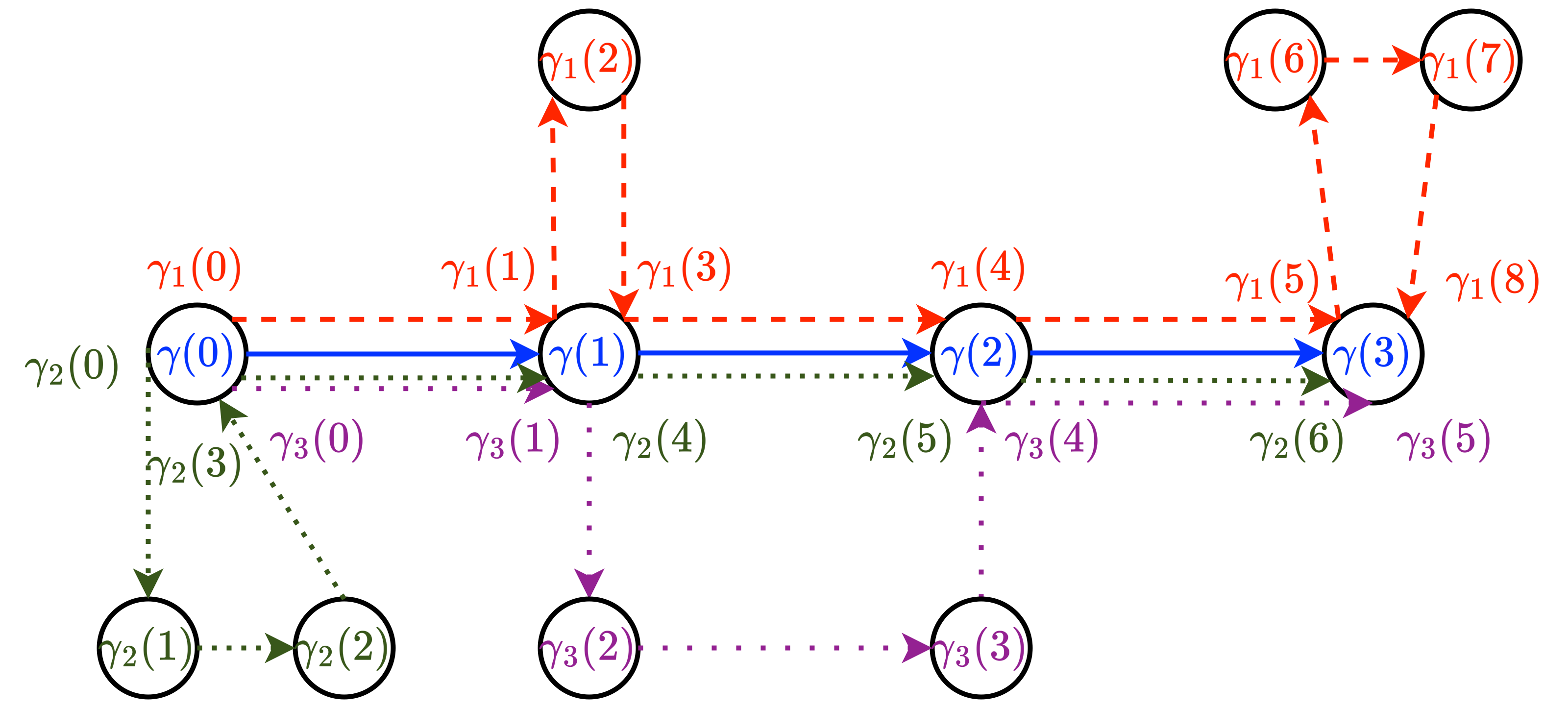
Figure 6: Example of Definition 4.5: here the paths $\gamma,\gamma_{1}$ and $\gamma_{2}$, represented respectively in plain blue, dashed red and dense dotted green, are equivalent. But the path $\gamma_{3}$, represented in sparse dotted purple, is not equivalent to any of the other paths. In particular it is not possible to construct a function $\sigma$ satisfying condition (ii) of Definition 4.5 for the path $\gamma_{3}$. We have that $|\gamma|=4$, $|\gamma_{1}|=9$, $|\gamma_{2}|=7$, and $\sigma_{1}(0)=(0,0)$, $\sigma_{1}(1)=(1,3)$, $\sigma_{1}(2)=(4,4)$, $\sigma_{1}(3)=(5,8)$, $\sigma_{2}(0)=(0,3)$, $\sigma_{2}(1)=(4,4)$, $\sigma_{2}(2)=(5,5)$ and $\sigma_{2}(3)=(6,6)$.

We introduce the notion of the mono-directional graph associated to a path $\gamma$ in the following definition.

Definition 4.6.

The mono-directional graph associated to a path $\gamma=(0,\gamma(1),\cdots,\gamma(k))$ is the graph $(V_{\gamma},E_{\gamma})$ where

$$V_{\gamma}:=\{0,\gamma(1),\cdots,\gamma(k)\},$$

$$E_{\gamma}:=\{(0,\gamma(1)),(\gamma(1),\gamma(2)),\cdots,(\gamma(k-1),\gamma(k))\}.$$

In other words it is the graph composed of the successive subpopulations $\big{(}Z_{(0)}^{(n)},Z_{(0,\gamma(1))}^{(n)},\cdots,Z_{\gamma}^{(n)}\big{)}$.

Now we have all the preliminary results and definitions to prove Theorem 2.7.

Proof of Theorem 2.7.

We show Equation (2.18) and (2.20). The proofs of Equations (2.19) and (2.21) are similar and is left to the reader.

Step 1: Let $\widetilde{\gamma}$ a representing candidate of a class of equivalence. Our first step is to prove, using the result of Section 3, that for all $\varepsilon>0$

$$\mathbb{P}\Big{(}\sup_{s\in[-M,M]}\sup_{t\in[0,T]}\Big{|}\sum_{\gamma\in[\widetilde{\gamma}]}\frac{Z_{\gamma}^{(n)}\big{(}\mathfrak{t}_{t}^{(n)}+s\big{)}}{d_{\widetilde{\gamma}}^{(n)}(t,s)}-Ww_{\widetilde{\gamma}}(t)\Big{|}\geq\varepsilon\Big{)}\underset{n\to\infty}{\longrightarrow}0,$$ (4.20)

where for all $\gamma\in\Gamma(V)$

$$d_{\gamma}^{(n)}(t,s):= \mathbbm{1}_{\left\{t\in[0,t(\gamma)-h_{n}^{-1}\right\}}+\mathbbm{1}_{\left\{t\in[t(\gamma)-h_{n}^{-1},t(\gamma))\right\}}\psi_{n}\log^{\theta(\gamma)-1}(n)$$ (4.21)

$$\hskip 56.9055pt+\mathbbm{1}_{\left\{t\in[t(\gamma),\infty)\right\}}n^{t-t(\gamma)}\log^{\theta(\gamma)}(n)e^{\lambda(0)s},$$ (4.22)

and $w_{\gamma}$ is defined in (2.9). Notice that

$$\mathbb{P}\Big{(}\sup_{s\in[-M,M]}\sup_{t\in[0,T]}\Big{|}\sum_{\gamma\in[\widetilde{\gamma}]}\frac{Z_{\gamma}^{(n)}\big{(}\mathfrak{t}_{t}^{(n)}+s\big{)}}{d_{\widetilde{\gamma}}^{(n)}(t,s)}-Ww_{\widetilde{\gamma}}(t)\Big{|}\geq\varepsilon\Big{)}$$ (4.23)

$$\leq\mathbb{P}\Big{(}\sup_{s\in[-M,M]}\sup_{t\in[0,T]}\Big{|}\frac{Z_{\widetilde{\gamma}}^{(n)}\big{(}\mathfrak{t}_{t}^{(n)}+s\big{)}}{d_{\widetilde{\gamma}}^{(n)}(t,s)}-Ww_{\widetilde{\gamma}}(t)\Big{|}\geq\varepsilon\Big{)}$$ (4.24)

$$+\sum_{\gamma\in[\widetilde{\gamma}]\backslash\{\widetilde{\gamma}\}:t(\gamma)\leq T}\mathbb{P}\Big{(}\sup_{s\in[-M,M]}\sup_{t\in[0,T]}\Big{|}\frac{Z_{\gamma}^{(n)}\big{)}\mathfrak{t}_{t}^{(n)}+s\big{)}}{d_{\widetilde{\gamma}}^{(n)}(t,s)}\Big{|}\geq\varepsilon\Big{)}$$ (4.25)

$$+\mathbb{P}\Big{(}\sup_{s\in[-M,M]}\sup_{t\in[0,T]}\sum_{\gamma\in[\widetilde{\gamma}]\backslash\{\widetilde{\gamma}\}:t(\gamma)>T}\Big{|}\frac{Z_{\gamma}^{(n)}\big{(}\mathfrak{t}_{t}^{(n)}+s\big{)}}{d_{\widetilde{\gamma}}^{(n)}(t,s)}\Big{|}\geq\varepsilon\Big{)}.$$ (4.26)

The term (4.24) is converging to 0 applying Equation (2.18) to the mono-directional graph given by the path $\widetilde{\gamma}$, as proven in Section 3. The term (4.25) converges also to $0$ since:

• the sum is on a finite set, because we are considering a finite graph with labels on the edges that are strictly positive,

• and for each $\gamma\in[\widetilde{\gamma}]\backslash\{\widetilde{\gamma}\}$ we have $t(\gamma)>t(\widetilde{\gamma})$ by definition of the representative (see Definition 4.5), which implies by applying Equation (2.18) on the mono-directional graph given by $\gamma$ that

  $$\mathbb{P}\Big{(}\sup_{s\in[-M,M]}\sup_{t\in[0,T]}\Big{|}\frac{Z_{\gamma}^{(n)}\big{(}\mathfrak{t}_{t}^{(n)}+s\big{)}}{d^{(n)}_{\widetilde{\gamma}}(t,s)}\Big{|}\geq\varepsilon\Big{)}\underset{n\to\infty}{\longrightarrow}0.$$ (4.27)

The term (4.26) converges to $0$ because

$$\mathbb{P}\Big{(}\sup_{s\in[-M,M]}\sup_{t\in[0,T]}\sum_{\gamma\in[\widetilde{\gamma}]\backslash\{\widetilde{\gamma}\}:t(\gamma)>T}Z_{\gamma}^{(n)}\big{(}\mathfrak{t}_{t}^{(n)}+s\big{)}=0\Big{)}\underset{n\to\infty}{\to}1.$$ (4.28)

Indeed we have for each $\gamma\in[\widetilde{\gamma}]\backslash\{\widetilde{\gamma}\}$ satisfying $t(\gamma)>T$ that

$$\mathbb{P}\Big{(}\sup_{s\in[-M,M]}\sup_{t\in[0,T]}Z_{\gamma}^{(n)}\big{(}\mathfrak{t}_{t}^{(n)}+s\big{)}=0\Big{)}\underset{n\to\infty}{\longrightarrow}1,$$ (4.29)

by applying Lemma 3.6 to the mono-directional graph given by $\gamma$. It remains to deal with the sum over the set $A_{\widetilde{\gamma}}(T):=\left\{\gamma\in[\widetilde{\gamma}]\backslash\{\widetilde{\gamma}\}:t(v)>T\right\}$. The easiest situation is when $|A_{\widetilde{\gamma}}(T)|<\infty$, since the result follows directly. Such situation corresponds exactly to the case where there is no cycle on the graph structure $(V,E)$ for the vertices of $\widetilde{\gamma}$. Now consider the case $|A_{\widetilde{\gamma}}(T)|=\infty$. In this case even if for all $\gamma\in A_{\widetilde{\gamma}}(T)$ we have Equation (4.29) it does not necessary mean that Equation (4.28) is automatically satisfied. The result follows if one shows that it exists a finite subset $B_{\widetilde{\gamma}}(T)\subset A_{\widetilde{\gamma}}(T)$ such that

$$\mathbb{P}\Big{(}\sup_{s\in[-M,M]}\sup_{t\in[0,T]}\sum_{\gamma\in A_{\widetilde{\gamma}}(T)\backslash B_{\widetilde{\gamma}}(T)}Z_{\gamma}^{(n)}\big{(}\mathfrak{t}_{t}^{(n)}+s\big{)}=0\Big{|}E^{(n)}_{\widetilde{\gamma}}\Big{)}=1,$$ (4.30)

with $E^{(n)}_{\widetilde{\gamma}}:=\big{\{}\sup_{s\in[-M,M]}\sup_{t\in[0,T]}\sum_{\gamma\in B_{\widetilde{\gamma}}(T)}Z_{\gamma}^{(n)}\big{(}\mathfrak{t}_{t}^{(n)}+s\big{)}=0\big{\}}.$ Then we will show that $B_{\widetilde{\gamma}}(T)$ exists. $[\widetilde{\gamma}]$ is composed of the paths where for each vertex $v$ visited by $\widetilde{\gamma}$, there may have a cycle going back to $v$. Because there are only a finite number of vertices visited by $\widetilde{\gamma}$ and that the label on the vertices are strictly positive, it comes that the number of paths $\gamma\in A_{\widetilde{\gamma}}(T)$ where we have to control the event that they do not have any cells up to time $\mathfrak{t}_{T}^{(n)}+M$ is actually finite and is denoted by $B_{\widetilde{\gamma}}(T)$. Indeed, for all paths $\gamma\in A_{\widetilde{\gamma}}(T)\backslash B_{\widetilde{\gamma}}(T)$ it exists a path $\gamma_{1}\in B_{\widetilde{\gamma}}(T)$ such that cells from the subpopulation $Z_{\gamma}^{(n)}$ are cells that results from (potentially many) mutations of cells of subpopulation $Z_{\gamma_{1}}^{(n)}$. Hence if one controls that with high probability there is no cell generated up to time $\mathfrak{t}_{T}^{(n)}+M$ of the subpopulations indexed by $\gamma\in B_{\widetilde{\gamma}}^{(n)}$, which is actually the case because $B_{\widetilde{\gamma}}^{(n)}$ is finite, it automatically implies by the mechanistic construction of the process that under such event, almost surely there is no cell of the subpopulations indexed by $\gamma\in A_{\widetilde{\gamma}}^{(n)}\backslash B_{\widetilde{\gamma}}^{(n)}$, which is exactly Equation (4.30).

Step 2: In this step Equation (2.18) is proven. Notice that for $\gamma\in A(v)$, where $A(v)$ is defined in Definition 2.5, we have $d_{\gamma}^{(n)}(t,s)=d_{v}^{(n)}(t,s)$, and also $\gamma$ is the representing candidate $\widetilde{\gamma}$ of its class of equivalence. In particular it means that $\sum_{\gamma\in A(v)}w_{\gamma}(t)=\sum_{\widetilde{\gamma}\in C(v):\widetilde{\gamma}\in A(v)}w_{\widetilde{\gamma}}(t)$, where $C(v)$ is defined in Definition 4.5. Then the proof is obtained thanks to

$$\mathbb{P}\Big{(}\sup_{s\in[-M,M]}\sup_{t\in[0,T]}\Big{|}\frac{Z_{v}^{(n)}\big{(}\mathfrak{t}_{t}^{(n)}+s\big{)}}{d_{v}^{(n)}(t,s)}-W\sum_{\gamma\in A(v)}w_{\gamma}(t)\Big{|}\geq\varepsilon\Big{)}$$ (4.31)

$$\leq\sum_{\widetilde{\gamma}\in C(v):\widetilde{\gamma}\in A(v)}\mathbb{P}\Big{(}\sup_{s\in[-M,M]}\sup_{t\in[0,T]}\Big{|}\sum_{\gamma\in[\widetilde{\gamma}]}\frac{Z_{\gamma}^{(n)}\big{(}\mathfrak{t}_{t}^{(n)}+s\big{)}}{d_{\widetilde{\gamma}}^{(n)}(t,s)}-Ww_{\widetilde{\gamma}}(t)\Big{|}\geq\varepsilon\Big{)}$$ (4.32)

$$+\sum_{\widetilde{\gamma}\in C(v):\widetilde{\gamma}\notin A(v)}\mathbb{P}\Big{(}\sup_{s\in[-M,M]}\sup_{t\in[0,T]}\Big{|}\sum_{\gamma\in[\widetilde{\gamma}]}\frac{Z_{\gamma}^{(n)}\big{(}\mathfrak{t}_{t}^{(n)}+s\big{)}}{d_{v}^{(n)}(t,s)}\Big{|}\geq\varepsilon\Big{)}.$$ (4.33)

Indeed, (4.32) converges to 0 by applying Equation (4.20) and because the sum is finite. And (4.33) converges to 0 because the sum is finite and because for all $\widetilde{\gamma}\in C(v),\widetilde{\gamma}\notin A(v)$ we have either $t(\widetilde{\gamma})>t(v)$ or $\theta(\widetilde{\gamma})<\theta(v)$.

Step 3: We are going to prove in this step Equation (2.20). Following the proof of Proposition 3.12 when replacing $\eta_{t}^{(n)}$ by $\tau_{t}^{(n)}$ and where $W$ is defined as in (4.15) instead of (3.14), we obtain that for all $0<T_{1}<T_{2}$ and for all $\varepsilon>0$

$$\mathbb{P}\Big{(}\sup_{t\in[T_{1},T_{2}]}\big{(}\tau_{t}^{(n)}-\sigma_{t}^{(n)}\big{)}\leq\varepsilon\Big{|}W>0\Big{)}\underset{n\to\infty}{\longrightarrow}1.$$ (4.34)

Indeed because the number of vertices in the graph is finite and due to Step 2 we have shown that the total number of mutant cells $\sum_{v\in V\backslash\{0\}}Z_{v}^{(n)}\big{(}\mathfrak{t}^{(n)}_{t}+s\big{)}$ are negligible compared to the number of wild-type cells $Z_{(0)}^{(n)}\big{(}\mathfrak{t}^{(n)}_{t}+s\big{)}$ for any time interval $[T_{1},T_{2}]$ allowing to perform the reasoning of (3.215) and (3.216), such that it gives a straightforward adaptation of the proof of Proposition 3.12. By adapting the different proofs from Subsection 3.3 we obtain that for all $0<T_{1}<T_{2}$, $M>0$ and $\varepsilon>0$

$$\mathbb{P}\Big{(}\sup_{s\in[-M,M]}\sup_{t\in[T_{1},T_{2}]}\Big{|}\frac{Z_{v}^{(n)}\big{(}\rho_{t}^{(n)}+s\big{)}}{d_{v}^{(n)}(t,s)}-\mathbbm{1}_{\{W>0\}}w_{v}(t)\Big{|}\geq\varepsilon\Big{)}\underset{n\to\infty}{\longrightarrow}0.$$ (4.35)

∎

5 Convergence for the stochastic exponents (Theorem 2.9)

This section is devoted to the proof of Theorem 2.9. Recall that $\big{(}Z^{(n)}_{v},v\in V\big{)}_{n\in\mathbb{N}}$ is mathematically constructed in Subsection 4 (see (4.6), (4.8) and (4.12)).

Step 1: We start by proving Theorem 2.9 conditioned on $\{W=0\}$. Let $0<T_{1}<T_{2}$, we are going to show that

$$\mathbb{P}\Big{(}\exists v\in V,\sup_{t\in[T_{1},T_{2}]}X_{v}^{(n)}(t)>0\Big{|}W=0\Big{)}\underset{n\to\infty}{\longrightarrow}0.$$ (5.1)

Introduce $\tau_{(0)}:=\inf\left\{s\in\mathbb{R}^{+}:Z_{(0)}(s)=0\right\}$ and $\tau_{(0)}^{(n)}:=\inf\big{\{}s\in\mathbb{R}^{+}:Z_{(0)}^{(n)}(s)=0\big{\}}$. Conditioned on $\{W=0\}$ we have $\tau_{(0)}^{(n)}\leq\tau_{(0)}<\infty$, as well as $Z_{(0)}(t)$ tends to $0$ when $t$ goes to infinity, almost surely. In particular one gets that for any function $f(n)\to\infty$ and any $\varepsilon>0$, $\mathbb{P}\left(Z_{(0)}(f(n))\geq\varepsilon\right)\to 0.$ Because $Z_{(0)}$ is an integer-valued process, if one takes epsilon strictly smaller than 1, one has shown that $\mathbb{P}\left(Z_{(0)}(f(n))=0\right)\to 1$. In particular it gives that $\mathbb{P}\big{(}\tau_{(0)}^{(n)}\geq T_{1}\tfrac{\log(n)}{\lambda(0)}\big{|}W=0\big{)}\underset{n\to\infty}{\longrightarrow}0.$ Moreover we have

$$\mathbb{P}\Big{(}\exists v\in V,\sup_{t\in[T_{1},T_{2}]}X_{v}^{(n)}(t)>0\Big{|}W=0\Big{)}\leq\mathbb{P}\Big{(}\tau_{(0)}^{(n)}\geq T_{1}\frac{\log(n)}{\lambda(0)}\Big{|}W=0\Big{)}$$ (5.2)

$$\hskip 28.45274pt+\mathbb{P}\Big{(}\bigcup_{v\in N(0)}\Big{\{}\sup_{t\geq 0}K^{(n)}_{(0),v}(t)>0\Big{\}}\bigcup_{(v,u)\in N(0)}\Big{\{}\sup_{t\geq 0}H^{(n)}_{(0),\{v,u\}}(t)>0\Big{\}}\Big{|}W=0\Big{)}.$$ (5.3)

Using a similar approach as in step 1 of the proof of Proposition 3.4, see the proof of Lemma 3.6, we prove that (5.3) converges to 0, which gives (5.1).

Step 2: Now we are going to prove the result of Theorem 2.9 conditioned on $\{W>0\}$.
We begin with the initial phase using the following Lemma.

Lemma 5.1.

By construction $\Delta_{1}=\underset{v\in N(0)}{\min}(\ell(0,v))>0$. Let $0<\varepsilon<\frac{\Delta_{1}}{2}$. For all $\widetilde{\varepsilon}>0$

$$\mathbb{P}\Big{(}\Big{\{}\sup_{t\in[\varepsilon,\Delta_{1}-\varepsilon]}\left|X^{(n)}_{0}(t)-\lambda_{0}t\right|\leq\widetilde{\varepsilon}\Big{\}}\cap\Big{\{}\sup_{v\in V\backslash\{0\}}\sup_{t\in[\varepsilon,\Delta_{1}-\varepsilon]}X_{v}^{(n)}(t)=0\Big{\}}\Big{|}W>0\Big{)}\underset{n\to\infty}{\longrightarrow}1.$$ (5.4)

Proof.

Using a similar approach as in the proof of Lemma 3.6 just by adapting the situation, one can prove that $\mathbb{P}\big{(}\sup_{v\in V\backslash\{0\}}\sup_{t\in[\varepsilon,\Delta_{1}-\varepsilon]}Z^{(n)}_{v}\big{(}\mathfrak{t}^{(n)}_{t}\big{)}=0\big{)}\underset{n\to\infty}{\to}1,$ from which it follows by definition of $X^{(n)}_{v}$ that

$$\mathbb{P}\Big{(}\sup_{v\in V\backslash\{0\}}\sup_{t\in[\varepsilon,\Delta_{1}-\varepsilon]}X^{(n)}_{v}\left(t\right)=0\Big{)}\underset{n\to\infty}{\longrightarrow}1.$$ (5.5)

We also have, by definition of $W$ as the almost sure limit of the positive martingale $\left(e^{-\lambda(0)t}Z_{(0)}(t)\right)_{t\in\mathbb{R}^{+}}$ and using Lemma 4.3, that for all $\bar{\varepsilon}>0$, $\mathbb{P}\big{(}A^{(n)}_{\bar{\varepsilon}}\big{)}\underset{n\to\infty}{\longrightarrow}1,$ with

$$A^{(n)}_{\bar{\varepsilon}}:=\Big{\{}\sup_{t\in\left[\mathfrak{t}^{(n)}_{\varepsilon},\mathfrak{t}^{(n)}_{\Delta_{1}-\varepsilon}\right]}|e^{-\lambda^{(n)}(0)t}Z_{0}^{(n)}(t)-W|\leq\bar{\varepsilon}\Big{\}}.$$

Indeed, as mentioned above with high probability there is no mutational event from the lineage of cells $Z_{(0)}^{(n)}$, meaning that with high probability $Z_{0}^{(n)}(t)=Z_{(0)}^{(n)}(t),\forall t\in\big{[}\mathfrak{t}^{(n)}_{\varepsilon},\mathfrak{t}^{(n)}_{\Delta_{1}-\varepsilon}\big{]}.$ Let $\delta>0$, $\bar{\varepsilon}<\delta$, conditioned on $\{W>\delta\}$ one obtains that for all $\omega\in A^{(n)}_{\bar{\varepsilon}}$ and for all $t\in[\varepsilon,\Delta_{1}-\varepsilon]$

$$(W-\bar{\varepsilon})e^{\lambda^{(n)}(0)\mathfrak{t}^{(n)}_{t}}\leq Z_{0}^{(n)}\Big{(}\mathfrak{t}^{(n)}_{t}\Big{)}\leq(W+\bar{\varepsilon})e^{\lambda^{(n)}(0)\mathfrak{t}^{(n)}_{t}},$$ (5.6)

which implies because it exists an $n\in\mathbb{N}$ independent from the value of $W$ such that $(W-\bar{\varepsilon})e^{\lambda^{(n)}(0)\mathfrak{t}^{(n)}_{t}}\geq 1$ that

$$\frac{\log(W-\bar{\varepsilon})\lambda(0)}{\log(n)}+\lambda^{(n)}(0)t\leq X_{0}^{(n)}(t)\leq\frac{\log(W+\bar{\varepsilon})\lambda(0)}{\log(n)}+\lambda^{(n)}(0)t.$$ (5.7)

Then because $\lambda^{(n)}(0)\underset{n\to\infty}{\to}\lambda(0)$ it gives that

$$\mathbb{P}\Big{(}\Big{\{}\sup_{t\in[\varepsilon,\Delta_{1}-\varepsilon]}\Big{|}X_{0}^{(n)}(t)-\lambda(0)t\Big{|}\leq\widetilde{\varepsilon}\Big{\}}\cap\Big{\{}\sup_{v\in V\backslash\{0\}}\sup_{t\in[\varepsilon,\Delta_{1}-\varepsilon]}X_{v}^{(n)}(t)=0\Big{\}}\Big{|}W>\delta\Big{)}$$ (5.8)

$$\underset{n\to\infty}{\longrightarrow}1.$$ (5.9)

The result is ended applying a similar reasoning as in Step 2 of the proof of Lemma 3.2, allowing to switch the conditioning from $\{W>\delta\}$ to $\{W>0\}$. ∎

Then we are going to express how the asymptotic behavior of $\big{(}X_{v}^{(n)}\big{)}_{v\in V}$ is controlled between the times $\Delta_{j}$ for $j\in\{1,\cdots,k^{*}\}$.

Lemma 5.2.

Let $j\in\{1,\cdots,k^{*}-1\}$ and $0<\varepsilon<\frac{\Delta_{j+1}-\Delta_{j}}{2}$. Assume that $\big{(}X_{v}^{(n)}(\Delta_{j}+\varepsilon)\big{)}_{v\in V}$ converges in probability to $(x_{v}(\Delta_{j}+\varepsilon))_{v\in V}$. Then we have for all $\widetilde{\varepsilon}>0$

$$\mathbb{P}\Big{(}\sup_{v\in V}\sup_{t\in[\Delta_{j}+\varepsilon,\Delta_{j+1}-\varepsilon]}\Big{|}X_{v}^{(n)}(t)-x_{v}(t)\Big{|}\leq\widetilde{\varepsilon}\Big{|}W>0\Big{)}\underset{n\to\infty}{\longrightarrow}1.$$ (5.10)

Proof.

The proof of this Lemma is obtained by adapting the one of [3], Proposition 2, because the behavior of the models are similar between two times of change of slope. Indeed, in our case, the property of branching is satisfied, there is no interaction between individuals except mutational exchange. In [3] although there are interactions between individuals, the model is well approximated by branching populations between two changes of slope (corresponding to either a new born trait or either a change of the dominant trait) as in the present work. In their case, some assumptions on how the functions $(x_{v})_{v\in V}$ behaves are added to prevent that two different traits become dominant simultaneously. This is due to technicalities when coupling the processes with a three species Lotka-Volterra system. But in our case, everything is branching, this situation with a potential coupling with a competitive system does not arise such that this lemma is free from such assumptions. ∎

Finally we are going to show how the asymptotic behavior of $\big{(}X_{v}^{(n)}\big{)}_{v\in V}$ is controlled around times $\Delta_{j}$ for $j\in\{1,\cdots,k^{*}\}$. By adapting [3], Proposition 4, one shows the following Lemma.

Lemma 5.3.

Let $j\in\{1,\cdots,k^{*}\}$ and $0<\varepsilon<\frac{\Delta_{j}-\Delta_{j-1}}{2}$. Assume that $\big{(}X_{v}^{(n)}(\Delta_{j}-\varepsilon)\big{)}_{v\in V}$ converges in probability to $(x_{v}(\Delta_{j}-\varepsilon))_{v\in V}$. Then it exists $0<\bar{\varepsilon}<\frac{\Delta_{j+1}-\Delta_{j}}{2}$ such that for all $\widetilde{\varepsilon}>0$

$$\mathbb{P}\Big{(}\sup_{v\in V}\sup_{t\in[\Delta_{j}-\varepsilon,\Delta_{j}+\bar{\varepsilon}]}\Big{|}X_{v}^{(n)}(t)-x_{v}(t)\Big{|}\leq\widetilde{\varepsilon}\Big{|}W>0\Big{)}\underset{n\to\infty}{\longrightarrow}1,$$ (5.11)

where by convention one defines $\Delta_{k^{*}+1}=\infty$.

Proof.

The proof of this lemma is highly inspired from the one of Proposition 4 of [3]. This Proposition aims at dealing with the birth of a new trait. Moreover the techniques of the proof are still consistent if at the same time not only one but many new traits appeared. However in our case it may also happen that an already born trait $v$ increases its slope due to a growth driven now by another trait $u\neq v$. This was not studied in [3] because it never happens in their model. But in our case, such an event appears exactly when one of the subpopulations of trait $v$ whose growth is driven by another trait $u\neq v$ becomes now dominant inside the total population of the trait $v$. In particular, it means that if one would like to deal with this kind of event, one would have to track the birth of all the subpopulations over the paths on the graph from the origin. Hence the way the sequence $\big{(}Z_{v}^{(n)},v\in V\big{)}_{n\in\mathbb{N}}$ is constructed using sums of subpopulations over the paths on the graph from the origin, see Equations (4.6) and (4.8), allows to deal with such phenomenon only adapting Proposition 4 of [3]. Indeed instead of considering the set of traits as $V$, we are considering the set of traits as all the paths on the graph from the origin $\Gamma(V)$ and we apply the same reasoning using Lemma 5.1, Lemma 5.2 and the adaptation from Proposition 4 of [3] as mentioned above in this proof to get the result for this new set of traits $\Gamma(V)$.

With this in mind, we deduce that it exists $\widetilde{\Delta}_{0}=0<\widetilde{\Delta}_{1}<\cdots<\widetilde{\Delta}_{\widetilde{k}^{*}}$ such that the convergence on probability is obtained for the populations $\big{(}X_{\gamma}^{(n)}\big{)}_{\gamma\in\Gamma(V)}$ where

$$X_{\gamma}^{(n)}:=\frac{\log_{+}\big{(}Z_{\gamma}^{(n)}\big{(}\mathfrak{t}_{t}^{(n)}\big{)}\big{)}}{\log(n)/\lambda(0)},$$ (5.12)

to some deterministic functions $\left(x_{\gamma}\right)_{\gamma\in\Gamma(V)}$. In particular the set of traits $\Gamma(V)$ is potentially an infinite set if there are cycles, meaning that $\widetilde{\Delta}_{\widetilde{k}^{*}}$ is infinite. But we obtain results on finite time interval $[T_{1},T_{2}]$, thus only a finite number of populations $Z_{\gamma}^{(n)}$ are going to have at least a cell in this time interval, meaning that the situation is similar to the one of a finite trait space. Then if in the original process at time $\Delta_{j}$ a trait $v$ is increasing its slope, it means that it exists a time $\widetilde{\Delta}_{\widetilde{j}}<\Delta_{j}$ such that the subpopulation of trait $v$ becoming dominant in the total population of trait $v$ at time $\Delta_{j}$ was born at time $\widetilde{\Delta}_{\widetilde{j}}$ and lived sufficiently long $\big{(}\Delta_{j}-\widetilde{\Delta}_{\widetilde{j}}\big{)}$ such that it becomes dominant. This ends the proof of this Lemma.

∎

Proof of Lemma 3.5.

For all $t\geq 0$ let $\mathcal{F}_{i,t}^{(n)}$ the $\sigma$-field generated by $Z^{(n)}_{j}(s)$ for $0\leq j\leq i$ and $0\leq s\leq t$. For all $h\geq 0$ we have

$$\mathbb{E}\Big{[}M_{i}^{(n)}(t+h)-M_{i}^{(n)}(t)|\mathcal{F}_{i,t}^{(n)}\Big{]}=\mathbb{E}\Big{[}Z^{(n)}_{i}(t+h)\Big{\lvert}\mathcal{F}_{i,t}^{(n)}\Big{]}e^{-\lambda_{i}^{(n)}(t+h)}$$ (.13)

$$\hskip 56.9055pt-Z^{(n)}_{i}(t)e^{-\lambda_{i}^{(n)}t}-\int_{t}^{t+h}2\alpha_{i-1}\mu_{i-1}^{(n)}e^{-\lambda_{i}^{(n)}s}\mathbb{E}\Big{[}Z^{(n)}_{i-1}(s)\Big{\lvert}\mathcal{F}_{i,t}^{(n)}\Big{]}ds.$$ (.14)

The forward Chapman-Kolmogorov equation gives the time-differential equation

$$\begin{split}\dfrac{d\mathbb{E}\Big{[}Z^{(n)}_{i}(t)\Big{]}}{dt}=\lambda_{i}^{(n)}\mathbb{E}\Big{[}Z^{(n)}_{i}(t)\Big{]}+2\alpha_{i-1}\mu_{i-1}^{(n)}\mathbb{E}\Big{[}Z^{(n)}_{i-1}(t)\Big{]},\end{split}$$ (.15)

which leads to

$$\mathbb{E}_{Z_{i}^{(n)}(0)}\Big{[}Z^{(n)}_{i}(t)\Big{]}=Z^{(n)}_{i}(0)e^{\lambda_{i}^{(n)}t}+\int_{0}^{t}2\alpha_{i-1}\mu_{i-1}^{(n)}\mathbb{E}_{Z_{i}^{(n)}(0)}\Big{[}Z^{(n)}_{i-1}(s)\Big{]}e^{\lambda_{i}^{(n)}(t-s)}ds.$$ (.16)

In particular using the Markov property we obtain that

$$\mathbb{E}\Big{[}Z^{(n)}_{i}(t+h)\Big{\lvert}\mathcal{F}_{i,t}^{(n)}\Big{]}=Z^{(n)}_{i}(t)e^{\lambda_{i}^{(n)}h}+\int_{t}^{t+h}2\alpha_{i-1}\mu_{i-1}^{(n)}\mathbb{E}\Big{[}Z^{(n)}_{i-1}(s)\lvert\mathcal{F}_{i,t}^{(n)}\Big{]}e^{\lambda_{i}^{(n)}(t+h-s)}ds.$$ (.17)

Combining (.13) and (.17) it follows that $\big{(}M_{i}^{(n)}(t)\big{)}_{t\in\mathbb{R}^{+}}$ is a martingale. Let $F^{(n)}(t,x,y):=(e^{-\lambda_{i}^{(n)}t}x-y)^{2}$, it follows that $\frac{\partial F^{(n)}}{\partial t}(t,x,y)=-2\lambda_{i}^{(n)}xe^{-\lambda_{i}^{(n)}t}\sqrt{F^{(n)}(t,x,y)}$ and $\frac{\partial F^{(n)}}{\partial y}(t,x,y)=-2\sqrt{F^{(n)}}.$ Applying Itô’s formula with $x=Z_{i}^{(n)}(t)$ and $y=\int_{0}^{t}2\alpha_{i-1}\mu_{i-1}^{(n)}e^{-\lambda_{i}^{(n)}s}Z^{(n)}_{i-1}(s)ds$ we obtain

$$\Big{(}M^{(n)}_{i}(t)\Big{)}^{2}=F^{(n)}\Big{(}t,Z_{i}^{(n)}(t),\int_{0}^{t}2\alpha_{i-1}\mu_{i-1}^{(n)}e^{-\lambda_{i}^{(n)}s}Z^{(n)}_{i-1}(s)ds\Big{)}$$ (.18)

$$=F^{(n)}(0,0,0)-2\int_{0}^{t}2\alpha_{i-1}\mu_{i-1}^{(n)}e^{-\lambda_{i}^{(n)}s}Z^{(n)}_{i-1}(s)M^{(n)}_{i}(s)ds-2\lambda_{i}^{(n)}\int_{0}^{t}e^{-\lambda_{i}^{(n)}s}Z^{(n)}_{i}(s)M^{(n)}_{i}(s)ds$$ (.19)

$$+\int_{0}^{t}\int_{\mathbb{R}^{+}}\Big{[}\Big{(}M_{i}^{(n)}(s^{-})+e^{-\lambda_{i}^{(n)}s}\Big{\{}\mathbbm{1}_{\left\{\theta\leq\alpha_{i}^{(n)}Z^{(n)}_{i}(s^{-})\right\}}-\mathbbm{1}_{\left\{\alpha_{i}^{(n)}Z_{i}^{(n)}(s^{-})\leq\theta\leq\left(\alpha_{i}^{(n)}+\beta_{i}\right)Z_{i}^{(n)}(s^{-})\right\}}\Big{\}}\Big{)}^{2}$$ (.20)

$$\hskip 227.62204pt-\Big{(}M_{i}^{(n)}(s^{-})\Big{)}^{2}\Big{]}Q_{i}(ds,d\theta)$$ (.21)

$$+\int_{0}^{t}\int_{\mathbb{R}^{+}}\Big{[}\Big{(}M_{i}^{(n)}(s^{-})+e^{-\lambda_{i}^{(n)}s}\mathbbm{1}_{\left\{\theta\leq 2\alpha_{i-1}\mu_{i-1}^{(n)}\left(1-\mu_{i-1}^{(n)}\right)Z_{i-1}^{(n)}(s^{-})\right\}}\Big{)}^{2}-\Big{(}M_{i}^{(n)}(s^{-})\Big{)}^{2}\Big{]}N_{i-1}(ds,d\theta)$$ (.22)

$$+\int_{0}^{t}\int_{\mathbb{R}^{+}}\Big{[}\Big{(}M_{i}^{(n)}(s^{-})+e^{-\lambda_{i}^{(n)}s}2\mathbbm{1}_{\left\{\theta\leq\alpha_{i-1}\left(\mu_{i-1}^{(n)}\right)^{2}Z_{i-1}^{(n)}(s^{-})\right\}}\Big{)}^{2}-\Big{(}M_{i}^{(n)}(s^{-})\Big{)}^{2}\Big{]}Q_{i-1}^{m}(ds,d\theta)$$ (.23)

$$+\int_{0}^{t}\int_{\mathbb{R}^{+}}\Big{[}\Big{(}M_{i}^{(n)}(s^{-})-e^{-\lambda_{i}^{(n)}s}\mathbbm{1}_{\left\{\theta\leq\alpha_{i}\left(\mu_{i}^{(n)}\right)^{2}Z_{i}^{(n)}(s^{-})\right\}}\Big{)}^{2}-\Big{(}M_{i}^{(n)}\Big{)}^{2}\Big{]}Q_{i}^{m}(s^{-})(ds,d\theta)$$ (.24)

$$=-2\int_{0}^{t}\left(2\alpha_{i-1}\mu_{i-1}^{(n)}Z^{(n)}_{i-1}(s)+\lambda_{i}^{(n)}Z^{(n)}_{i}(s)\right)e^{-\lambda_{i}^{(n)}s}M^{(n)}_{i}(s)ds$$ (.25)

$$+2\int_{0}^{t}\left(2\alpha_{i-1}\mu_{i-1}^{(n)}Z^{(n)}_{i-1}(s)+\lambda_{i}^{(n)}Z^{(n)}_{i}(s)\right)e^{-\lambda_{i}^{(n)}s}M^{(n)}_{i}ds$$ (.26)

$$+\int_{0}^{t}\left[2\alpha_{i-1}\mu_{i-1}^{(n)}Z^{(n)}_{i-1}(s)+\left(\alpha_{i}^{(n)}+\beta_{i}^{(n)}\right)Z^{(n)}_{i}(s)\right]e^{-2\lambda_{i}^{(n)}s}ds+\widetilde{M}^{(n)}_{i}(t)$$ (.27)

$$=\widetilde{M}^{(n)}_{i}(t)+\int_{0}^{t}2\alpha_{i-1}\mu_{i-1}^{(n)}e^{-2\lambda_{i}^{(n)}s}Z_{i-1}^{(n)}(s)ds+\left(\alpha_{i}^{(n)}+\beta_{i}^{(n)}\right)\int_{0}^{t}e^{-2\lambda_{i}^{(n)}s}Z_{i}^{(n)}(s)ds,$$ (.28)

where $\widetilde{M}^{(n)}_{i}$ is a martingale. Finally, we get

$$\Big{\langle}M^{(n)}_{i}\Big{\rangle}_{t}=\int_{0}^{t}2\alpha_{i-1}\mu_{i-1}^{(n)}e^{-2\lambda_{i}^{(n)}s}Z_{i}^{(n)}(s)ds+\Big{(}\alpha_{i}^{(n)}+\beta_{i}^{(n)}\Big{)}\int_{0}^{t}e^{-2\lambda_{i}^{(n)}s}Z_{i}^{(n)}(s)ds.$$ (.29)

∎

Proof of Lemma 3.9.

First we have that $\mathbb{E}\big{[}Z_{0}^{(n)}(u)\big{]}=e^{\lambda_{0}^{(n)}u}\leq e^{\lambda_{0}u}$, which is exactly the result for $i=0$. Then for $i\in\mathbb{N}$ assume that the result is true for $i-1$. Then taking the expectation of the martingale $M_{i}^{(n)}$ defined in (3.51) at time $u$ and using the previous assumption we obtain the following equation

$$\mathbb{E}\Big{[}Z_{i}^{(n)}(u)\Big{]} \leq e^{\lambda_{i}u}\int_{0}^{u}2\alpha_{i-1}\mu_{i-1}^{(n)}e^{-\lambda_{i}s}\mathbb{E}\Big{[}Z_{i-1}^{(n)}(s)\Big{]}ds$$ (.30)

$$\leq C_{i-1}\mu_{\otimes,i}^{(n)}2\alpha_{i-1}\int_{0}^{u}e^{(\lambda_{0}-\lambda_{i})s}dsu^{\theta(i-1)}e^{\lambda_{i}u}$$ (.31)

$$\leq C_{i-1}\mu_{\otimes,i}^{(n)}2\alpha_{i-1}\Big{(}\mathbbm{1}_{\{\lambda_{i}=\lambda_{0}\}}u+\mathbbm{1}_{\{\lambda_{i}<\lambda_{0}\}}\frac{1}{\lambda_{0}-\lambda_{i}}e^{\left(\lambda_{0}-\lambda_{i}\right)u}\Big{)}u^{\theta(i-1)}e^{\lambda_{i}u}$$ (.32)

$$=C_{i-1}\mu_{\otimes,i}^{(n)}2\alpha_{i-1}\Big{(}\mathbbm{1}_{\{\lambda_{i}=\lambda_{0}\}}+\mathbbm{1}_{\{\lambda_{i}<\lambda_{0}\}}\frac{1}{\lambda_{0}-\lambda_{i}}\Big{)}u^{\theta(i)}e^{\lambda_{0}u},$$ (.33)

which concludes the proof by induction. ∎

Proof of Lemma 3.10.

In the proof $C$ corresponds to a strictly positive constant that may change from line to line.

Neutral case: Assume that $\lambda_{i}=\lambda_{0}$. Applying Lemma 3.9, remembering that $\lambda_{i}^{(n)}=\lambda_{0}-2\alpha_{i}\mu_{i}^{(n)}$, and using that it exists $N_{1}\in\mathbb{N}$ such that for all $n\geq N_{1}$ we have that $e^{4\alpha_{i}\mu_{i}^{(n)}\left(\mathfrak{t}^{(n)}_{t_{2}}+s\right)}\leq 2$, we obtain that

$$\int_{\mathfrak{t}^{(n)}_{t_{1}^{(n)}}+s}^{\mathfrak{t}^{(n)}_{t_{2}}+s}e^{-2\lambda_{i}^{(n)}u}\mathbb{E}\Big{[}Z_{i}^{(n)}(u)\Big{]}du \leq C\mu_{\otimes,i}^{(n)}\int_{\mathfrak{t}^{(n)}_{t_{1}^{(n)}}+s}^{\mathfrak{t}^{(n)}_{t_{2}}+s}u^{\theta(i)}e^{-\lambda_{0}u}du.$$ (.34)

Using an integration by parts we obtain that

$$\int_{\mathfrak{t}^{(n)}_{t_{1}^{(n)}}+s}^{\mathfrak{t}^{(n)}_{t_{2}}+s}u^{\theta(i)}e^{-\lambda_{0}u}du\leq\frac{1}{\lambda(0)}\big{(}\mathfrak{t}^{(n)}_{t^{(n)}_{1}}+s\big{)}^{\theta(i)}e^{-\lambda_{0}\big{(}\mathfrak{t}^{(n)}_{t^{(n)}_{1}}+s\big{)}}+\frac{\theta(i)}{\lambda_{0}}\int_{\mathfrak{t}^{(n)}_{t_{1}^{(n)}}+s}^{\mathfrak{t}^{(n)}_{t_{2}}+s}u^{\theta(i)-1}e^{-\lambda_{0}u}du.$$ (.35)

Then using $\theta(i)$ integration by parts, it exists $N_{2}\in\mathbb{N}$ such that for $n\geq N_{2}$ we have

$$\int_{\mathfrak{t}^{(n)}_{t_{1}^{(n)}}+s}^{\mathfrak{t}^{(n)}_{t_{2}}+s}u^{\theta(i)}e^{-\lambda_{0}u}du\leq C\frac{e^{-\lambda_{0}s}}{n^{t_{1}^{(n)}}}\big{(}\mathfrak{t}^{(n)}_{t_{1}^{(n)}}+s\big{)}^{\theta(i)}.$$ (.36)

It follows that for $n\geq\max(N_{1},N_{2})$

$$\int_{\mathfrak{t}^{(n)}_{t_{1}^{(n)}}+s}^{\mathfrak{t}^{(n)}_{t_{2}}+s}e^{-2\lambda_{i}^{(n)}u}\mathbb{E}\Big{[}Z_{i}^{(n)}(u)\Big{]}du \leq C\frac{e^{-\lambda_{0}s}}{n^{t_{1}^{(n)}}}\mu_{\otimes,i}^{(n)}\big{(}\mathfrak{t}^{(n)}_{t_{1}^{(n)}}+s\big{)}^{\theta(i)}.$$ (.37)

Because the vertex $i$ is assumed to be neutral it follows that $\theta(i-1)=\theta(i)-1$. Using similar computation as the latter one, it exists $N_{3}\in\mathbb{N}$ such that for $n\geq N_{3}$ we have

$$\int_{\mathfrak{t}^{(n)}_{t_{1}^{(n)}}+s}^{\mathfrak{t}^{(n)}_{t_{2}}+s}\mu_{i-1}^{(n)}e^{-2\lambda_{i}^{(n)}u}\mathbb{E}\Big{[}Z_{i-1}^{(n)}(u)\Big{]}du\leq C\frac{e^{-\lambda_{0}s}}{n^{t_{1}^{(n)}}}\mu_{\otimes,i}^{(n)}\big{(}\mathfrak{t}^{(n)}_{t_{1}^{(n)}}+s\big{)}^{\theta(i)-1}.$$ (.38)

It follows that for all $n\geq\max(N_{1},N_{2},N_{3})$ we have

$$\mathbb{E}\Big{[}\big{\langle}M_{i}^{(n)}\big{\rangle}_{\mathfrak{t}^{(n)}_{t_{2}}+s}-\big{\langle}M_{i}^{(n)}\big{\rangle}_{\mathfrak{t}^{(n)}_{t_{1}^{(n)}}+s}\Big{]} \leq C\frac{e^{-\lambda_{0}s}}{n^{t_{1}^{(n)}}}\mu_{\otimes,i}^{(n)}\big{(}\mathfrak{t}^{(n)}_{t_{1}^{(n)}}+s\big{)}^{\theta(i)}.$$ (.39)

Deleterious case: We now deal with the case $\lambda_{i}<\lambda_{0}$ by applying the same strategy. We obtain

$$\int_{\mathfrak{t}^{(n)}_{t_{1}^{(n)}}+s}^{\mathfrak{t}^{(n)}_{t_{2}}+s}e^{-2\lambda_{i}^{(n)}u}\mathbb{E}\Big{[}Z_{i}^{(n)}(u)\Big{]}du\leq C\mu_{\otimes,i}^{(n)}\int_{\mathfrak{t}^{(n)}_{t_{1}^{(n)}}+s}^{\mathfrak{t}^{(n)}_{t_{2}}+s}u^{\theta(i)}e^{\left(\lambda_{0}-2\lambda_{i}\right)u}du$$ (.40)

$$\hskip 56.9055pt\leq C\mu_{\otimes,i}^{(n)}\left(\mathfrak{t}^{(n)}_{t_{2}}+s\right)^{\theta(i)}\Big{[}\mathbbm{1}_{\{\lambda_{0}>2\lambda_{i}\}}e^{\left(\lambda_{0}-2\lambda_{i}\right)\left(\mathfrak{t}^{(n)}_{t_{2}}+s\right)}$$ (.41)

$$\hskip 113.81102pt+\mathbbm{1}_{\{\lambda_{0}=2\lambda_{i}\}}\big{(}\mathfrak{t}^{(n)}_{t_{2}}+s\big{)}+\mathbbm{1}_{\{\lambda_{i}<\lambda_{0}<2\lambda_{i}\}}e^{-\left(2\lambda_{i}-\lambda_{0}\right)\big{(}\mathfrak{t}^{(n)}_{t_{1}^{(n)}}+s\big{)}}\Big{]}.$$ (.42)

Then remembering that $\theta(i-1)=\theta(i)$, we get that

$$\int_{\mathfrak{t}^{(n)}_{t_{1}^{(n)}}+s}^{\mathfrak{t}^{(n)}_{t_{2}}+s}\mu_{i-1}^{(n)}e^{-2\lambda_{i}^{(n)}u}\mathbb{E}\Big{[}Z_{i-1}^{(n)}(u)\Big{]}du\leq C\mu_{\otimes,i}^{(n)}\big{(}\mathfrak{t}^{(n)}_{t_{2}}+s\big{)}^{\theta(i)}\Big{[}\mathbbm{1}_{\{\lambda_{0}>2\lambda_{i}\}}e^{\left(\lambda_{0}-2\lambda_{i}\right)(\mathfrak{t}^{(n)}_{t_{2}}+s)}$$ (.43)

$$\hskip 113.81102pt+\mathbbm{1}_{\{\lambda_{0}=2\lambda_{i}\}}\big{(}\mathfrak{t}^{(n)}_{t_{2}}+s\big{)}+\mathbbm{1}_{\{\lambda_{i}<\lambda_{0}<2\lambda_{i}\}}e^{-\left(2\lambda_{i}-\lambda_{0}\right)\big{(}\mathfrak{t}^{(n)}_{t_{1}^{(n)}}+s\big{)}}\Big{]}.$$ (.44)

At the end we have

$$\mathbb{E}\Big{[}\big{\langle}M_{i}^{(n)}\big{\rangle}_{\mathfrak{t}^{(n)}_{t_{2}}+s}-\big{\langle}M_{i}^{(n)}\big{\rangle}_{\mathfrak{t}^{(n)}_{t_{1}^{(n)}}+s}\Big{]}\leq C\mu_{\otimes,i}^{(n)}\big{(}\mathfrak{t}^{(n)}_{t_{2}}+s\big{)}^{\theta(i)}\cdot\Big{[}\mathbbm{1}_{\{\lambda_{0}>2\lambda_{i}\}}e^{\left(\lambda_{0}-2\lambda_{i}\right)(\mathfrak{t}^{(n)}_{t_{2}}+s)}$$ (.45)

$$\hskip 56.9055pt+\mathbbm{1}_{\{\lambda_{0}=2\lambda_{i}\}}\big{(}\mathfrak{t}^{(n)}_{t_{2}}+s\big{)}+\mathbbm{1}_{\{\lambda_{i}<\lambda_{0}<2\lambda_{i}\}}e^{-\left(2\lambda_{i}-\lambda_{0}\right)\big{(}\mathfrak{t}^{(n)}_{t_{1}^{(n)}}+s\big{)}}\Big{]}.$$ (.46)

∎

Acknowledgements

The author would like to thank Hélène Leman for inspiring and helpful discussions as well as feedback. The author would like to thank the Chair ”Modélisation Mathématique et Biodiversité” of VEOLIA-Ecole Polytechnique-MNHN-F.X.

Funding

This research was led with financial support from ITMO Cancer of AVIESAN (Alliance Nationale pour les Sciences de la Vie et de la Santé, National Alliance for Life Sciences Health) within the framework of the Cancer Plan.

References

[1]Jones, S., Chen, W., Parmigiani, G., Diehl, F., Beerenwinkel, N., Antal, T., Traulsen, A., Nowak, M., Siegel, C., Velculescu, V., and others (2008).
Comparative lesion sequencing provides insights into tumor evolution
Proceedings of the National Academy of Sciences105 4283–4288
[2]Bozic, I. and Nowak, M. (2014).
Timing and heterogeneity of mutations associated with drug resistance in metastatic cancers.
Proceedings of the National Academy of Sciences45 15964–15968
[3]Durrett, R. and Mayberry, J. (2011).
Traveling waves of selective sweeps.
Ann. Appl. Probab.21 699–744
[4]Smadi, C. (2017).
The effect of recurrent mutations on genetic diversity in a large population of varying size.
Acta Applicandae Mathematicae149 11–51
[5]Cheek,D. and Antal, T. (2018).
Mutation frequencies in a birth-death branching process.
Ann. Appl. Probab.28 3922–3947
[6]Bovier, A., Coquille, L. and Smadi, C. (2019).
Crossing a fitness valley as a metastable transition in a stochastic population model.
Ann. Appl. Probab.29 3541–3589
[7]Cheek,D. and Antal, T. (2020).
Genetic composition of an exponentially growing cell population.
Stochastic Process. Appl.130 6580–6624
[8]Champagnat, N., Méléard, S. and Tran, V. C. (2021).
Stochastic analysis of emergence of evolutionary cyclic behavior in population dynamics with transfer.
Ann. Appl. Probab.31 1820–1867
[9]Coquille, L., Kraut, A. and Smadi, C. (2021).
Stochastic individual-based models with power law mutation rate on a general finite trait space.
Electron. J. Probab.26 1–37
[10]Esser, M. and Kraut, A. (2021).
A general multi-scale description of metastable adaptive motion across fitness valleys.
arXiv preprint arXiv:2112.12675
[11]Blath, J., Paul, T. and Tóbiás, A. (2023).
A Stochastic Adaptive Dynamics Model for Bacterial Populations with Mutation, Dormancy and Transfer.
ALEA, Lat. Am. J. Probab. Math. Stat.20 313-357
[12]Paul, T. (2023).
The canonical equation of adaptive dynamics in individual-based models with power law mutation rates.
arXiv preprint arXiv:2309.02148
[13]Gamblin, J., Gandon, S., Blanquart, F. and Amaury, L. (2023).
A Stochastic Adaptive Dynamics Model for Bacterial Populations with Mutation, Dormancy and Transfer.
Genetics224 iyad001
[14]Esser, M. and Kraut, A. (2023).
Effective growth rates in a periodically changing environment: From mutation to invasion.
arXiv preprint arXiv:2310.20509
[15]Sottoriva, A., Kang, H., Ma, Z., Graham, T., Salomon, M., Zhao, J., Marjoram, P., Siegmund, K., Press, M., Shibata, D., and others (2015).
A Big Bang model of human colorectal tumor growth.
Nature genetics47 209–216
[16]Ling, S., Hu, Z., Yang, Z., Yang, F., Li, Y., Li, P., Chen, K., Dong, L., Cao, L., Tao, Y., and others (2015).
Extremely high genetic diversity in a single tumor points to prevalence of non-Darwinian cell evolution.
Proceedings of the National Academy of Sciences112 E6496–E6505
[17]Williams, M. J., Werner, B., Barnes, C. P., Graham, T. A. and Sottoriva, A. (2016).
Identification of neutral tumor evolution across cancer types.
Nature genetics48 238–244
[18]Venkatesan, S. and Swanton, C. (2016).
Tumor evolutionary principles: how intratumor heterogeneity influences cancer treatment and outcome.
American Society of Clinical Oncology Educational Book36 e141–e149
[19]Davis, A., Gao, R. and Navin, N. (2017).
Tumor evolution: Linear, branching, neutral or punctuated?
Biochimica et Biophysica Acta (BBA)-Reviews on Cancer36 e141–e149
[20]Zeng, K., Fu, Y., Shi, S. and Wu, C. (2006).
Statistical tests for detecting positive selection by utilizing high-frequency variants.
Genetics174 1431–1439
[21]Achaz, G. (2009).
Frequency spectrum neutrality tests: one for all and all for one.
Genetics183 249–258
[22]Gunnarsson, E. B., Leder, K. and Foo, J. (2021).
Frequency spectrum neutrality tests: one for all and all for one.
Theoretical population biology142 67–90
[23]Luria, S. E. and Delbrük, M. (1943).
Mutations of bacteria from virus sensitivity to virus resistance.
Genetics28 491
[24]Lea, D. E. and Coulson, C. A. (1949).
The distribution of the numbers of mutants in bacterial populations.
Journal of genetics49 264–285
[25]Kendall, D. G. (1960).
Birth-and-death processes, and the theory of carcinogenesis.
Biometrika47 113–21
[26]Hamon, A. and Ycart, B. (2012).
Statistics for the Luria-Delbrück distribution.
Electronic Journal of Statistics6 1251-1272
[27]Keller, P. and Tibor, A. (2015).
Mutant number distribution in an exponentially growing population.
Journal of Statistical Mechanics: Theory and Experiment2015 P01011
[28]Kessler, D. A. and Levine, H. (2015).
Scaling solution in the large population limit of the general asymmetric stochastic Luria–Delbrück evolution process.
Journal of statistical physics158 783–805
[29]Nicholson, M. and Tibor, A. (2019).
Competing evolutionary paths in growing populations with applications to multidrug resistance.
PLoS computational biology15 e1006866
[30]Nicholson, M., Cheek, D. and Tibor, A. (2023).
Sequential mutations in exponentially growing populations.
PLoS computational biology19 e1011289
[31]Gunnarsson, E. B., Leder, K. and Zhang, X. (2023).
Limit theorems for the site frequency spectrum of neutral mutations in an exponentially growing population.
arXiv preprint arXiv:2307.03346
[32]Foo, J. and Leder, K. (2013).
Dynamics of cancer recurrence.
Ann. Appl. Probab.23 1437–1468
[33]Durrett, R. and Moseley, S. (2010).
Evolution of resistance and progression to disease during clonal expansion of cancer.
Theoretical population biology77 42–48
[34]Durrett, R. (2015).
Branching process models of cancer.
Springer.
[35]Le Gall, J. (2016).
Brownian motion, martingales, and stochastic calculus.
Springer.
[36]Dellacherie, C. and Mayer, P. (1975).
Probabilités et Potentiel.
Collection Enseignement des Sciences. Hermann, Paris.