S-GBDT: Frugal Differentially Private Gradient Boosting Decision Trees

Abstract

Privacy-preserving learning of gradient boosting decision trees (GBDT) has the potential for strong utility-privacy tradeoffs for tabular data, such as census data or medical meta data: classical GBDT learners can extract non-linear patterns from small sized datasets. The state-of-the-art notion for provable privacy-properties is differential privacy, which requires that the impact of single data points is limited and deniable. We introduce a novel differentially private GBDT learner and utilize four main techniques to improve the utility-privacy tradeoff. (1) We use an improved noise scaling approach with tighter accounting of privacy leakage of a decision tree leaf compared to prior work, resulting in noise that in expectation scales with $O(1/n)$, for $n$ data points. (2) We integrate individual Rényi filters to our method to learn from data points that have been underutilized during an iterative training process, which – potentially of independent interest – results in a natural yet effective insight to learning streams of non-i.i.d. data. (3) We incorporate the concept of random decision tree splits to concentrate privacy budget on learning leaves. (4) We deploy subsampling for privacy amplification.

Our evaluation shows an improvement of up to a factor 66 in terms of epsilon: For the Abalone dataset ($<4k$ training data points), we achieve $R^{2}$-score of $0.39$ for $\varepsilon=0.15$, which the closest prior work only achieved for $\varepsilon=10.0$. On the Adult dataset ($50k$ training data points) we achieve test error of $18.7\,\%$ for $\varepsilon=0.07$ which the closest prior work only achieved for $\varepsilon=1.0$. For the Abalone dataset for $\varepsilon=0.54$ we achieve $R^{2}$-score of $0.47$ which is very close to the $R^{2}$-score of $0.54$ for the nonprivate version of GBDT. For the Adult dataset for $\varepsilon=0.54$ we achieve test error $17.1\,\%$ which again is very close to the test error $13.7\,\%$ of the nonprivate version of GBDT.

I Introduction

Gradient boosting decision tree ensembles (GBDT) achieve strong machine learning performance on highly-nonlinear tabular data tasks, such as tasks based on sensitive census data or sensitive medical records. GBDTs utilize a robust, data-efficient, incremental learning method, traits that are optimal for strong privacy-preserving approximations. These models combine many weak decision tree learners into an ensemble to prevent overfitting while still capturing complex non-linear patterns.

Figure 1: $\varepsilon$-DP S-GBDT greatly outperforms prior work (DPBoost [13]) and comes close to the nonprivate baseline. Evaluated on abalone regression dataset with $<4k$ training points. Higher coefficient of determination R2 is better.

In some applications training data is highly sensitive. Classical decision trees are vulnerable to privacy attacks on training data. Each tree consists of splits and leaves which are data-dependent and thus potentially leak information. This leakage potential manifests in practice, as GDBT trees are typically significantly overfitted. The state-of-the-art notion for provably protecting against such information leakage is differential privacy (DP), which requires that the impact of single data points be small and deniable.

Prior work on learning decision tree ensembles with DP either did not consider GBDTs [4], or provides suboptimal utility-privacy tradeoffs [13]. The most promising prior work is the DPBoost learner from Li et al. [13]. DPBoost, however, unnecessarily causes leakage in learning good splits, while our result show that it is more promising to spend the privacy budget on learning leaves and more trees. Moreover, DPBoost is based on an untight accounting for the privacy leakage, resulting in a suboptimal utility-privacy tradeoff. DPBoost, furthermore, utilizes parallel composition instead of subsampling, which has been proven to provide stronger utility-privacy tradeoff than parallel composition.

Contributions  We introduce the novel DP-GBDT algorithm S-GBDT which comes close to the nonprivate baseline even for medium-sized datasets ($<4k$ data points). We compare S-GBDT to a version of DPBoost [13] that we enhanced by adding a DP initial score and by performing a hyperparameter search. In terms of the privacy parameter $\varepsilon$, S-GBDT is better than the enhanced DPBoost up to a factor of 66: On the Abalone dataset, we achieve R2-score of 0.39 for $\varepsilon=0.15$, which DPBoost only achieved for $\varepsilon=10.0$. On the Adult dataset we achieve test error of $18.7\,\%$ for $\varepsilon=0.07$ which DPBoost only achieved for $\varepsilon=1.0$.

S-GBDT facilities this privacy enhancement through four key contributions:

1. We use an adaptive noise scaling with tighter accounting of privacy leakage of a decision tree leaf compared to prior work, such that the scale is in expectation in $O(1/n)$ for $n$ data points (c.f. Section VI-B), compared to $O(1)$ in prior work [13].

2. We present a method for learning on streams of non-i.i.d. data, where we consecutively update the model with new data throughout the training of the model. For learning on streams of non-i.i.d. data, we propose tailoring a so-called individual Renyi filter [10] to DP-GBDT training, which can also boost performance in regular training (c.f. Section VI-F).

3. To further boost utility-privacy, we utilize subsampling [1, 19] instead of parallel composition as proposed by Li et al. [13] (c.f. Section VI-C).

4. We compare S-GBDT to DPBoost (c.f. Section V-B and c.f. for the experiments Section VIII). We enhance DPBoost [13] by adding a DP initial score, performing a hyperparameter search, and utilizing a gridless exponential mechanism (potentially of independent interest).
   In terms of the privacy parameter $\varepsilon$, S-GBDT is better than the enhanced DPBoost up to a factor of 66: on the Abalone dataset, we achieve $R^{2}$-score of 0.39 for $\varepsilon=0.15$, which DPBoost only achieved for $\varepsilon=10.0$. For the Abalone dataset for $\varepsilon=0.54$ we achieve $R^{2}$-score of $0.47$ which is very close to the $R^{2}$-score of $0.54$ for the nonprivate version of GBDT (cf. Figure 1). For the Adult dataset for $\varepsilon=0.54$ we achieve a test error of $17.1\,\%$ which is close to the test error $13.7\,\%$ of the nonprivate version of GBDT. Furthermore, we perform ablation studies for S-GBDT on our dynamic leaf noise scaling approach and on the individual Rényi filter that is tailored to the S-GBDT training.

5. Our ablation studies show that the technique of gradient-based data filtering (GDF) introduced by Li et al. [13] does not provide any improvement (c.f. Section VIII-F).

II Overview

We propose S-GBDT: a fast, explainable, and non-linear ML model that is differentially private (cf. main Theorem 11) while losing little utility compared to a non-differentially private ML model. S-GBDT builds on the gradient boosting decision trees (GBDTs) paradigm (c.f. Section IV-B). A schematic overview is given in Figure 2.

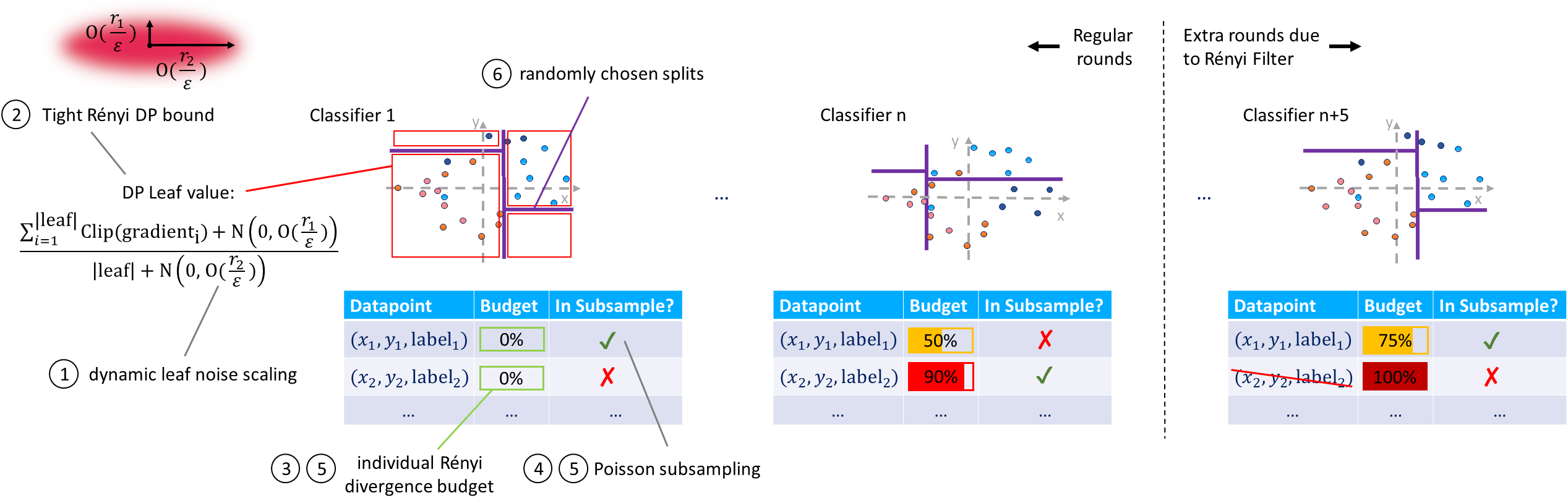
Figure 2: Schematic overview of S-GBDT learning a regression task on a two-dimensional dataset. The colors of data points represent their gradients. For the DP leaf value, $\text{Clip}(\text{gradient}_{i})$ means a clipped version of the gradient, $\varepsilon$ is the privacy budget and $r_{1},r_{2}$ allow to shift the noise arbitrarily between the numerator and the denominator ($r_{1},r_{2}>0$, $r_{1}+r_{2}=1)$. The numbers ➀ to ➅ refer to our key technical features for S-GBDT (c.f. Section II).

Decision trees split the inputs according to their features at each inner node and as a prediction use the value at the leaf at which a data point lands. The main sources of leakage for decision tree ensembles are choosing the best splits and choosing the best leaves. Moreover, when training several trees we have to be careful not to unnecessarily use the same information repeatedly, as that could amplify privacy leakage. Gradient boosting is a technique for minimizing the unnecessary repeated use of the same information. We deploy several further techniques to minimize privacy leakage.

From a high-level viewpoint, S-GBDT reaches a robust privacy-utility tradeoff through the following key insights. Items ➀ - ➅ are our key technical features.

➀ Dynamic leaf noise scaling  We use an improved noise scaling approach with tighter accounting of privacy leakage of a decision tree leaf compared to prior work, resulting in noise that in expectation scales with $O(1/n)$, for $n$ data points (c.f Section VI-B). We achieve this by not only releasing the sum over gradients in a leaf but also releasing the leaf support in a differentially private manner. We allow the noise scale to be shifted between both values and tightly account for the privacy leakage of our approach by analytically deriving a Rényi DP bound.

➁ Analytical Rényi DP bound for Gaussian mechanism with non-spherical noise  Our differentially private algorithm for computing the leaves of trees in a DP-GBDT ensemble is of independent interest, as we show a general result on how to utilize the Gaussian mechanism with non-spherical (anisotropic) noise (c.f Section VI-B). This allows jointly releasing multiple statistics on the same subsample in a differentially private manner, while calibrating the noise to each statistic specifically, with potential for better utility compared to the classic multivariate Gaussian mechanism, which scales the noise for each statistic equally.

➂ Tailoring individual Rényi filter to DP-GBDT  We tailor an individual Rényi filter [10] to the training of DP-GBDTs to leverage individual privacy accounting (c.f Section VI-F). Individual privacy accounting enables training for as many rounds as desired while still preserving an a priori bound on the individual Rényi DP privacy loss. This technique boosts utility while bringing individuals’ privacy loss closer to the global privacy budget that is obtained through a worst case analysis rather than an individual analysis (cf. Figure 3 for a visual interpretation).

Figure 3: Individual Rényi Filter (IRF) boosts the average privacy leakage (dotted line) on the abalone dataset. We measure on a data-point-level how much the gradient sum of a S-GBDT leaf changes when removing one data point. Then, we aggregate this per-data-point-leakage across the ensemble. While the graph does not show a formal worst-case privacy guarantee, it visualizes that IRF better uses the available budget. For IRF, we use 100 extra trees.

➃ Poisson subsampled tree learning  We utilize subsampling, which randomly samples a subset from the dataset for each training round (c.f Section VI-C). This allows data points to be used in training of multiple trees, yielding good utility, while also giving strong deniability as an adversary does not know whether a data point was used in training of a tree. This deniability leads to a privacy amplification by subsampling which roughly states that, given a subsampling probability $\gamma$ with which a data point is added to a subsample from the dataset and a $(\varepsilon,\delta)$-differentially private algorithm, its subsampled variant satisfies $(O(\gamma\varepsilon),\gamma\delta)$-differential privacy  [2].

➄ Subsampling and individual Rényi filter  We combine both techniques of an individual Rényi filter and privacy amplification by subsampling by analyzing subsampled individual Rényi differential privacy. Our Rényi DP accountant can measure the privacy budget spent by individuals over multiple rounds of subsampled training in terms of Rényi DP (c.f. Section VI-E). Subsampled Rényi DP facilitates the boost to the privacy-utility tradeoff when compared to standard parallel and sequential composition for differential privacy that is utilized in closest prior work  [13].

➅ Random tree splits  During GBDT training, the leaves and splits of each trained tree are data-dependent and thus incur privacy leakage. Yet, it suffices for a reasonable utility drop to only train leaves data-dependent. This means that we choose the splits randomly to save any privacy budget spent on the leaves (c.f. Section VI-C). The concept of random splits is supported by Bojarski et al. [4] who show utility guarantees in a theoretical analysis for a random forest (RF) setup. They argue that often a few trees have by chance reasonable splits and these suffice to bias the trees enough for a high-quality prediction. Closest prior work utilizes the exponential mechanism to choose tree splits while preserving differential privacy, but for the number of possible split candidates, the exponential mechanism will likely draw from an almost uniform distribution as well.

➆ Addressing secondary privacy leakages & improvements  There are secondary privacy leakages beyond the primary leakage of leaves and splits in a tree. Yet, closest prior work does not investigate the following secondary privacy leakages and does not implement improvements. (1) The initial score improves the GBDT training by providing a first estimate of the prediction: for regression, it is the average over regression labels from the training dataset. We enable using an initial score by releasing this average in a differentially private manner (c.f. Section VI-D). (2) The original DPBoost algorithm uses as split-candidates a grid, which is computationally inefficient. We introduce a more efficient grid-less exponential mechanism, with the same performance, and apply it to DPBoost. (3) A feature border consists of a lower and upper bound on the values of a feature from the training dataset. It has not been accounted for in prior work. This feature border is relevant for random splits to set up an interval from which to sample, and it is also relevant for splits based on a gain function, where split candidates are chosen from an interval of possible values. In our experiments, we use a static feature border for all features (c.f. Section VI-C). (4) Besides splits and leaves, an attacker is also able to observe data-dependent changes in the tree layout. We eliminate such leakage by always training a tree fully i.e. we mock up splits and leaves even when no data point from training data would end up in such a leaf (c.f Section VI-C).

➇ Gradient-based data filtering  Our experiments show that the technique of gradient-based data filtering introduced by Li et al. [13] does not provide any improvement (c.f.  Section VIII-F).

II-A Application Areas

S-GBDT is amenable to two non-trivial application areas:

Learning on streams of non-i.i.d. data via an individual Rény filter  When learning on streams of non-i.i.d. data, we consecutively update the model with new data throughout its training. Especially such new data points that arrive late in the training phase of the model, can only have little influence on the model, resulting in bad overall accuracy. Tailoring individual Rényi filters to the training of DP-GBDTs, allows to keep training with new data points, yielding a natural yet effective insight to learning on streams of non-i.i.d. data (c.f. Section VIII-E).

Scalable distributed learning  Our differentially private training algorithm for GBDT works seamlessly with distributed learning (c.f. Section IX), a setting where multiple parties jointly train a model, without divulging their respective private training datasets to any other user or the public. This is especially relevant in the field of sensitive medical meta data that hospitals might want to keep at their hospital but still want to use to train a machine learning model collaboratively with other hospitals with their own share of sensitive data.

III Related work

Our work concentrates on GBDTs as a data-frugal ML technique, which does not need a large amount of data for strong utility-privacy tradeoffs. Prior work on learning decision tree ensembles in DP includes an algorithm by Bojarski et al. [4] to learn random forests in DP and a work by Li et al. [13] to learn gradient boosting decision tree ensembles in DP.

The work by Bojarski et al. [4] proposes to use many random splits instead of learning a few good splits. That work proves utility bounds for randomly choosing splits, yet does not utilize the potential of gradient boosting ensemble learning, subsampling and individual Rényi filters.

Closest to our results is the work by Li et al. [13] for learning gradient boosting decision tree ensembles (GBDT) in a differentially private manner. We give an overview over their algorithm in  Section V-B. Li et al. propose to use the exponential mechanism for finding strong splits and introduce a novel technique, called gradient-based data filtering. Gradient-based data filtering filters out data points with large gradients and leaves them for later trees, hoping that these points will have a smaller gradient when training later trees. We experimentally show, however, that their gradient-based data filtering does not provide any improvement. Further, their work does not use a differentially private initial score, which can improve GBDT learning, it does not utilize privacy amplification methods, and has a leaf noise scale that does not decrease with the number of data points. As a result, we do not consider the work of Li et al. to be data-frugal.

Other data-frugal learners are SVMs or other ML techniques with convex optimization techniques. They also achieve strong utility-privacy tradeoffs with few data points [6]. Yet, compared to convex learners, GBDTs are able to learn highly non-linear problems.

IV Preliminaries

Symbol	Description
$M$	Randomized mechanism
$X$ or $D$	Dataset
$X\sim X^{\prime}$	Neighboring datasets
$X\sim_{x}X^{\prime}$	Neighoring datasets
	differing in $x$
$(\varepsilon,\delta)$	Approximate DP bound
$D_{\alpha}^{\leftrightarrow}(M(X)||M(X^{\prime}))$	Rényi Divergence of order $\alpha$
$(\alpha,\rho(\alpha))$	Rényi DP bound $\rho(\alpha)$
	of order $\alpha$
$(\alpha,\rho_{t}^{(i)}(\alpha))$	Individual Rényi DP bound
	of data point $x_{i}$ for round $t$
$\mathcal{F}_{\alpha,\rho(\alpha)}$	Individual Rényi filter
$x\in X$	Data point
$y_{i}$	Label of data point $x_{i}$
$\tilde{y_{i}}$	Predicted label of
	data point $x_{i}$
$g_{i}$	Gradient of data point $x_{i}$
$o$	Observation

TABLE I: Notation Table

IV-A Differential privacy

Differential privacy  [9] is the de-facto standard for provable privacy. For some mechanism that generates data-dependent output, differential privacy requires that the impact of single data points is limited and deniable. Like closest prior work  [13], we consider unbounded differential privacy, where the effect of adding or removing a single instance from a dataset on the output is analyzed. We utilize Rényi differential privacy, as it is more convenient mathematically.

Definition 1 (Neighboring datasets).

Let $X,X^{\prime}\subseteq\mathcal{X}$ be two datasets. $X,X^{\prime}$ are neighboring, denoted by $X\sim X^{\prime}$ if $X^{\prime}=X\cup\{x\}$ for some $x\in\mathcal{X}$. If the two datasets differ in a specific $x_{i}\in\mathcal{X}$, this is denoted as $X\sim_{x_{i}}X^{\prime}$.

Definition 2 ($(\varepsilon,\delta)$- Differential Privacy,  [9]).

A randomized mechanism $M:\mathcal{X}\mapsto\mathcal{R}$ satisfies $(\varepsilon,\delta)$-differential privacy if, for any two neighboring datasets $X\sim X^{\prime}$ and any observation $o$ of $M$

$$\Pr[M(X)=o]\leq e^{\varepsilon}\cdot\Pr[M(X^{\prime})=o]+\delta$$

Definition 3 (Rényi Divergence,  [15]).

Let $P,Q$ be two probability distributions defined over $\mathcal{R}$. The Rényi divergence of order $\alpha$ is defined as

$$D_{\alpha}^{\leftrightarrow}(P||Q):=\frac{1}{\alpha-1}\log\int_{\infty}^{-\infty}\frac{P(x)^{\alpha}}{Q(x)^{\alpha-1}}dx$$

Definition 4 (Rényi Differential Privacy,  [14] Definition 4).

Privacy] A randomized mechanism $M:\mathcal{X}\mapsto\mathcal{R}$ satisfies $(\alpha,\rho(\alpha))$-Rényi differential privacy if, for any two neighboring datasets $X\sim X^{\prime}$

$$D_{\alpha}^{\leftrightarrow}(M(X)||M(X^{\prime})\leq\rho(\alpha)$$

IV-B Gradient boosting decision trees

GBDT  [11] is an ensemble learning technique that combines many weak learners (decision trees) in a sequential fashion.

For a given labeled dataset with $n$ data points and $m$ features $\mathcal{D}=\{(x_{1},y_{1}),\ldots,(x_{n},y_{n})\}\subseteq\mathbb{R}^{m}\times\mathbb{R}$, a tree ensemble model $\phi$ is trained to minimize the objective

$$\mathcal{L}(\phi)=\sum_{i}l(\tilde{y}_{i},y_{i})+\sum_{k}\Omega(f_{k})$$

where $l$ is a differentiable convex loss function that measures the difference between the prediction $\tilde{y}_{i}$ and the label $y_{i}$, and $\Omega(f_{k})=\frac{1}{2}\lambda\lVert V\rVert^{2}$ is a regularization term on the leafs.

$\phi$ uses $k$ trees to predict the output $\tilde{y}_{i}$ for $x_{i}$:

$$\tilde{y}_{i}=\phi(x_{i})=\sum_{t=1}^{k}\eta f_{t}(x_{i})$$

where $\eta$ is the learning rate and $(f_{t})_{t=1}^{k}$ are the trees of $\phi$.

Each tree $f_{t}$ ($t=1,2,...,k)$ is built from the root down to the leaves, each node splitting the dataset when further going down the tree. For some node, assume that a split $s$ in this node splits the instances of the dataset $D$ into two disjoint sets: the left set $I_{L,s,D}$ and the right set $I_{R,s,D}$. The utility of a split is given by

$$G(I_{L,s,D},I_{R,s,D})=\frac{\Big{(}\sum_{x_{i}\in I_{L,s,D}}g_{i}\Big{)}^{2}}{|I_{L,s,D}|+\lambda}+\frac{\Big{(}\sum_{x_{i}\in I_{R,s,D}}g_{i}\Big{)}^{2}}{|I_{R,s,D}|+\lambda}$$

where each $g_{i}$ is set to be $g_{i}=\frac{\partial l(y_{i},\tilde{y}_{i})}{\partial\tilde{y}_{i}}$ in round $t$ where $\tilde{y}_{i}$ is the ensemble-prediction in round $t-1$, and $\lambda$ is a regularization parameter. GBDT training traverses all features and all splits to find the optimal split and continues to insert new splits until a stopping criterion is met. The leaves of $f_{t}$ contain the tree’s prediction, which is computed as

$$V(I_{D}):=-\frac{\sum_{x_{i}\in I_{D}}g_{i}}{|I_{D}|+\lambda}$$

for a subset $I_{D}$ of training data $D$ that ended up in this leaf.

Note that, for the case of the loss function $l$ being the mean-squared-error loss function, the gradient $g_{i}$ of some data point $(x_{i},y_{i})$ can simply be evaluated as the difference between the actual label and the prediction of the ensemble, i.e. $g_{i}:=y_{i}-\tilde{y}_{i}$.

IV-C Exponential mechanism

The exponential mechanism [8] offers a differentially private way to select from a set of candidates weighted by a utility function, which provides a score for each candidate. Given a utility function $u:\mathcal{X}\times\mathcal{R}\mapsto\mathbb{R}$ that is $\Delta_{u}$-sensitivity bounded with respect to input $X\in\mathcal{X}$, the exponential mechanism $M$ outputs a candidate $r\in\mathcal{R}$ with probability

$$\Pr[M(X,u)=r]=\frac{\exp(\varepsilon\cdot u(X,r)\frac{1}{2\Delta_{u}})}{\sum_{r^{\prime}\in\mathcal{R}}\exp(\varepsilon\cdot u(X,r^{\prime})\frac{1}{2\Delta_{u}})}$$

where $\varepsilon$ is the privacy budget.

Theorem 5 (Exponential mechanism,  [8] Theorem 3.10).

The exponential mechanism satisfies $\varepsilon$-differential privacy.

IV-D Randomized splits for trees

Trees of a GBDT ensemble with randomized splits can still yield good utility [4]. Randomized splits are constructed by choosing a split for each inner node of the tree randomly, i.e. randomly selecting a feature of the dataset and then randomly selecting a value for that feature to perform the split on. For a numerical feature $i$, we assume that a feature range $(v^{(i)}_{\min},v^{(i)}_{\max})$ is given, from which the value is sampled. The leaves are then constructed data-dependent as with regular decision trees in GBDT.

We intuitively explain why random splits yield good utility for the case of randomized decision trees for binary classification: As the trees in the ensemble are random, most trees do not provide useful splits that help in deciding the class for a sample from the dataset. This yields an almost even distribution between trees that predict class 0 and trees that predict class 1. By chance however, there will be a few decision trees that provide useful splits in predicting the class of samples from the test dataset. These trees tilt the prediction of the ensemble towards the right class.

IV-E Individual Rényi filter

The conventional privacy accounting approach involves a worst-case analysis of the privacy loss, assuming the global sensitivity for all individuals. This results in an overly conservative estimation of the privacy loss, as often datapoints with substantial support in the dataset have individual sensitivity that is smaller than the global sensitivity and only datapoints with less support in the dataset utilize the full sensitivity.

An individual Rényi filter  [10], is a way to implement personalized privacy accounting. The Rényi filter measures privacy losses individually via individual Rényi Differential Privacy ( Definition 6) and guarantees that no datapoint’s privacy loss will surpass a predefined upper bound $\rho(\alpha)$. This enables a differentially private mechanism, comprising a composed sequence of mechanisms $\mathcal{A}_{1},\mathcal{A}_{2},...,\mathcal{A}_{k}$, to execute as many rounds as desired using datapoints that have not expended their privacy budget, as long as the accounting for individual Rényi privacy losses is sound.

Definition 6 (Individual Rényi Differential Privacy).

Fix $n\in\mathbb{N}$ and a data point $x$. A randomized algorithm $\mathcal{A}$ satisfies $(\alpha,\rho(\alpha))$-individual Rényi differential privacy if for all neighboring datasets $D_{0},D_{1}$ that differ in $x_{i}$, denoted as $D_{0}\sim_{x_{i}}D_{1}$, and satisfy $|D_{0}|,|D_{1}|\leq n$, it holds that

$$D_{\alpha}^{\leftrightarrow}(\mathcal{A}(D_{0})||\mathcal{A}(D_{1})\leq\rho(\alpha)$$

Algorithm 1 describes the functionality of the individual Rényi filter. The algorithm obtains the individual Rényi privacy loss of round $t$ for each datapoint $i$ (line 1). Next, the algorithm filters out all the datapoints that have surpassed the predefined upper bound on the privacy loss $\rho(\alpha)$ (line 1) using the privacy filter from  Theorem 7 and then continues execution of $A_{t}$ in round $t$ only on the active data points that have not been filtered out. Feldman and Zrnic show, that  Algorithm 1 satisfies $(\alpha,\rho(\alpha))$-Rényi DP (c.f.  Theorem 8).

Theorem 7 (Rényi Privacy Filter, [10] Theorem 4.3).

Let

$$\mathcal{F}_{\alpha,\rho(\alpha)}(\rho_{1},\rho_{2},\dots,\rho_{k})=\begin{cases}\text{CONT, if $\sum_{i=1}^{k}\rho_{i}(\alpha)\leq\rho(\alpha)$}\\ \text{HALT, if $\sum_{i=1}^{k}\rho_{i}(\alpha)>\rho(\alpha)$}\end{cases}$$

where $\rho(\alpha)$ is the upper bound on the privacy loss and $\rho_{i}(\alpha)$ ($i\in\{1,2,\dots,k\}$) the individual privacy loss of a datapoint for round $i$. Then $\mathcal{F}_{\alpha,\rho}$ is a valid Rényi privacy filter.

Input: $D:\text{dataset}$

Input : $(\mathcal{A}_{1},\mathcal{A}_{2},\dots,\mathcal{A}_{k}):\text{sequence of algorithms}$

Input : $\hat{\alpha}:\text{R\'{e}nyi DP parameter}$

Input : $\rho(\hat{\alpha}):\text{upper bound on R\'{e}nyi DP privacy loss}$

1 for $t=1$ to $k$ do

2       for $x_{i}\in D$ do

3             $\rho_{t}^{(i)}(\alpha):=\sup{}_{X\sim{}_{x_{i}}X^{\prime}}D_{\alpha}^{\leftrightarrow}(\mathcal{A}_{t}(a_{1},\dots,a_{t-1},X)$ $||\mathcal{A}_{t}(a_{1},\dots,a_{t-1},X^{\prime}))$

4            

5      Determine active set $D_{t}=(x_{i}:\mathcal{F}_{\hat{\alpha},\rho(\hat{\alpha})}(\rho_{1}^{(i)},\rho_{2}^{(i)},\dots,\rho_{t}^{(i)})=\text{CONT})$

6       For all $x_{i}\in D$, set $\rho_{t}^{(i)}\leftarrow 0$ if $x_{i}\notin S_{t}$

7       Compute $a_{t}=\mathcal{A}_{t}(a_{1},\dots,a_{t-1},S_{t})$

return $(a_{1},a_{2},\dots,a_{k})$

Algorithm 1 Adaptive composition with individual privacy filtering (Algorithm 3  [10])

Theorem 8 (Adaptive Composition with Individual Privacy Filtering, [10] Theorem 4.5).

Adaptive composition with individual Rényi filters ( Algorithm 1) using the Rényi filter from  Theorem 7 satisfies $(\alpha,\rho(\alpha))$-Rényi differential privacy.

The proof of  Theorem 8 can be found in the paper by Feldman and Zrnic [10]. The intuition for the proof is that, whether a data point $x$ is active in some round, does not depend on the rest of the input dataset but only on the outputs of prior rounds, which are known to the adversary. Once $x$ is excluded from training, it does not lose any more privacy, because the output of any round from there on looks the same whether $x$ is present in the dataset or not.

IV-F Subsampled Rényi differential privacy

Privacy amplification by subsampling allows one to obtain a stronger privacy guarantee when choosing the datapoints for a single training round randomly from the training dataset rather than training on a fixed subset of the training dataset or even on the whole training dataset. Privacy amplification by subsampling was first analyzed by Li et al. [12]. In this work, we utilize Poisson Subsampling [2] where each datapoint is chosen according to a Bernoulli experiment with probability $\gamma$, to obtain a batch of training data. We utilize the bound of  Theorem 9 by Zhu et al.  [19] for subsampled Rényi DP.

Theorem 9 (Privacy Amplification by Subsampling,  [19], Theorem 6).

Let $\mathcal{M}$ be any randomized mechanism that obeys $(\alpha^{\prime},\rho^{\prime}(\alpha^{\prime}))$-Rényi differential privacy. Let $\gamma$ be the subsampling ratio and $\alpha\geq 2$. If $M^{\mathcal{P}_{\gamma}}=\mathcal{M}\circ\mathcal{P}_{\gamma}$ and $\mathcal{P}_{\gamma}$ generates a Poisson subsample with subsampling ratio $\gamma$, then $M^{\mathcal{P}_{\gamma}}$ is $(\alpha,\rho)$-Rényi differentially private with

$$\rho(\alpha)\leq\frac{1}{\alpha-1}\log{}\bigg{(} (1-\gamma)^{\alpha-1}(\alpha\gamma-\gamma+1)+$$

$$\binom{\alpha}{2}\gamma^{2}(1-\gamma)^{\alpha-2}e^{\rho^{\prime}(2)}+$$

$$3\sum_{l=3}^{\alpha}\binom{\alpha}{l}(1-\gamma)^{\alpha-l}\gamma^{l}e^{(l-1)\cdot\rho^{\prime}(l)}\bigg{)}$$

IV-G Secure aggregation

We utilize secure aggregation  [5] [3] to extend our DP-GBDT algorithm to distributed learning (c.f.  Section IX), a setting where $k$ users collaboratively train a machine learning model. Secure aggregation is a protocol for privately computing the sum of vectors

$$A=\sum_{u=1}^{k}W_{u}$$

where each user $u=1,2,...,k$ contributes a single vector $W_{u}$ and does not learn anything about the other users’ vectors other than the sum $A$.

V Improved split selection in DPBoost [13]

In regular GBDT training, we determine the optimal split using a gain metric from the mean squared error (MSE) family. Hereby, we calculate for every data point on every feature – we call this feature-value pair – a gain and split on the feature-value pair with the highest gain. Features either split on the “$=$” (categorical) or “$\leq$” comparison (numerical).

Closest prior work by Li et al. [13, Algorithm 1] proposes a differentially private split selection based on the exponential mechanism. However, their approach does not focus on addressing the secondary privacy leakages. Yet, these are indispensable to bridging the gap between theoretical requirements and validating implementations on real-world data and limited computational resources:

Their work assumes that the split selection candidates for the exponential mechanism are data-independent which is reasonable for categorical splits but computationally inefficient for numerical ones. For numerical features, they have to deploy a grid along the feature-value pairs. The more fine-grained the grid the better the utility, yet the worse the computational performance. Since the gain only changes when the split changes, in a best-case scenario we only need to compute as many split selection candidates as data points within a split.

V-A Grid-less exponential mechanism

Input: $D\in(\mathbb{R}\cup\mathbb{N})^{n\times k}$: input database on $k_{c}$ categorical and $k_{n}$ numerical features ($k\coloneqq k_{c}+k_{n}$)

Input : $(r^{(i)})_{i=1}^{k_{n}}\in\mathbb{R}_{+}^{k_{n}}$: numerical feature weights

Input : $(V^{(i)})_{i=k_{n}+1}^{k}$: categorical feature value vectors

Input : $u$: utility function with sensitivity $\Delta_{u}\in\mathbb{R}_{+}$

Input : $\varepsilon\in\mathbb{R}_{+}$: privacy parameter

Result: a sampled value $s$

$B\leftarrow$ List();

  // split candidate buckets

1 for each numerical feature $i,1\leq i\leq k_{n}$ do

2       $(v^{(i)})_{i=1}^{n}\leftarrow$ sort $D$ on feature $i$;

3       $B_{0}^{(i)}\leftarrow[v_{\textit{min}}^{(i)},v^{(i)}_{1})$; $B_{n+1}^{(i)}\leftarrow[v^{(i)}_{n},v_{\textit{max}}^{(i)}]$;

4       for each $j\in\{1,..,n\}$ do

5             $B_{j}^{(i)}\leftarrow[v_{j}^{(i)},v_{j+1}^{(i)})$;

6            

7      append $(B_{j}^{(i)})_{j=0}^{n+1}$ to $B$;

       $w^{(i)}\leftarrow\frac{r^{(i)}}{v_{\textit{max}}^{(i)}-v_{\textit{min}}^{(i)}}$;

        // feature weight

8      

9for each categorical feature $i,k-k_{c}\leq i\leq k$ do

10       for each feature split value $v^{(i)}_{j}\in V^{(i)}$ do

             $B_{j}^{(i)}\leftarrow[v^{(i)}_{j},v^{(i)}_{j}+1)$;

              // $\abs{B_{j}^{(i)}}=1$

11             append $B_{j}^{(i)}$ to $B$

      $w^{(i)}\leftarrow 1$;

        // feature weight

12      

13$Q\leftarrow\sum_{B_{a}^{(b)}\in B}w^{(b)}|B_{a}^{(b)}|\exp(\varepsilon\cdot u(B_{a}^{(b)},D)/{2\Delta_{u}})$;

14 $p_{j}^{(i)}\leftarrow{w^{(i)}|B_{j}^{(i)}|\exp(\varepsilon\cdot u(B_{j}^{(i)},D)/{2\Delta_{u}})}/Q$;

15 $B_{j}^{(i)}\sim\operatorname*{pmf}((p_{j}^{(i)})_{(i,j)=(1,0)}^{(k,n+1)})$;

16 if $B_{l}$ is numerical then

17       return $s\sim\operatorname*{Uniform}(\min B_{j}^{(i)},\max B_{j}^{(i)})$;

18      

19else

20       return $s\leftarrow\min B_{j}^{(i)}$;

21      

Algorithm 2 Grid-less Exponential Mechanism: G

To fix the computational shortcoming of a grid-full split selection, we propose a grid-less split selection which only needs to compute as many split selection candidates as there are data points within a split. Our grid-less split selection generalizes ExpQ [7, Algorithm 5] to a large class of utility functions and a combined selection of numerical and categorical features.

In Algorithm 2 we provide a generalized grid-less exponential mechanism that is of independent interest to other applications. In Algorithm 3 we show how we instantiate the grid-less exponential mechanism for the split selection use-case. Lemma 26 and Corollary 27 in the appendix show that both algorithms are $\varepsilon$-DP.

Input: $D\in\mathbb{R}^{n\times k}$: $n$-sized training data on $k_{c}$ categorical and $k_{n}$ numerical features ($k\coloneqq k_{c}+k_{n}$)

Input : $(v_{\textit{min}},v_{\textit{max}})\in\mathbb{R}^{2}$: numerical feature ranges

Input : $(V^{(i)})_{i=k_{n}+1}^{k}$: categorical feature values

Input : $r\in\mathbb{R}_{+}$: numerical feature weight

Input : $u$: MSE gain; $\Delta_{u}\in\mathbb{R}_{+}$: sensitivity of $u$

Result: $\varepsilon$-DP split value $s$ and corresponding feature

1 $\tilde{D}\leftarrow$ getDataOfCurrentTreeDepth($D$);

2 return $\textsc{G}(\tilde{D},(v_{\textit{min}},v_{\textit{max}})_{i=1}^{k_{n}},((r)_{i=1}^{k_{n}},(1)_{i=k_{c}+1}^{k}),$ return $($ $(V^{(i)})_{i=k_{n}+1}^{k},u,\Delta_{u},\varepsilon)$;

Algorithm 3 Improved split selection for DPBoost

V-B Overview of DPBoost

DPBoost trains an ensemble of decision trees by training each tree inside the ensemble on disjoint subsets of the training data. DPBoost trains multiple such ensembles on the full training dataset and composes all ensembles sequentially.

A single tree is trained by first iteratively creating splits for the tree via the exponential mechanism that privately selects a split from all split candidates, and then computing the leaves. To preserve privacy in the leaves, DPBoost adds to a leaf value Laplace noise that is calibrated to the clipping bound on the gradients $g^{*}$ and the privacy budget $\varepsilon_{\text{leaf}}$. DPBoost applies gradient-based data filtering, that filters out data points that have a gradient larger than the clipping bound and only trains a tree on the remaining data points, thus bounding the influence of data points on the tree splits and leaf values. DPBoost applies geometric leaf clipping to clip leaf values with a decreasing clipping bound to reduce the sensitivity of leaf values as the training progresses.

VI S-GBDT: Tighter DP-GBDT

VI-A Algorithm overview

We give a high-level description of our algorithm: S-GBDT begins by constructing a differentially private initial score on which the ensemble builds. S-GBDT then runs $T_{\max}$ training rounds where in each round we generate a Poisson subsample that the tree of the current round is trained on, giving our algorithm a privacy amplification by subsampling. When a single tree is trained, we choose the splits randomly to save privacy budget for the leaves. We compute the value of a leaf in a differentially private manner, where the required noise scales dynamically with the number of data points (the leaf support). We achieve this by releasing both the sum of gradients in a leaf and the leaf support via our adaptation of the differentially private Gaussian mechanism. Our adaptation allows for the noise to be shifted between the two released values, the gradient sum and the leaf support, facilitating optimal tuning of the noise. Finally, we tailor an individual Rényi filter to our algorithm to enable training of an arbitrary number of rounds, with only those datapoints that still have leftover individual privacy budget.

Theorem 11 shows $(\alpha,\rho(\alpha))$-Rényi DP for S-GBDT.

VI-B Leaf computation

Description of algorithm  S-GBDT computes a leaf for each tree in a GBDT ensemble using  Algorithm 4. First, we calculate and Gaussian noise the leaf support (line 4). Then, we calculate and Gaussian noise the sum of clamped gradients (line 4). With clamping we bound the influence of each gradient $g$ such that $\abs{g}\leq g^{*}$. We release a differentially private leaf value by dividing the noised sum of gradients by the noised leaf support.

Input: $l$: leaf node identifier

Input : $D:\text{training data}$

Input : $g\in D$ : gradients of data points in $D$

Input : $g^{*}$ : gradient clipping bound

Input : $\sigma_{\text{leaf}}^{2}$ : unweighted variance of Gaussian noise for leaves

1

2 Let $D_{l}\subseteq D$ be the set of data points in leaf $l$

3 $n=\sum_{g\in D_{l}}1$

4 $\tilde{n}=\text{{{max(}}{\emph{$\lambda,n+\text{{{Gauss(}}{\emph{$0.0,\sigma_{\text{leaf}}^{2}/(2\cdot r_{1})$}}{{)}}}$}}{{)}}}$

5 $s=\sum_{g\in D_{l}}\text{{{Clamp}}}(g,-g^{*},g^{*})$

6 $\tilde{s}=s+\text{{{Gauss(}}{\emph{$0.0,\sigma_{\text{leaf}}^{2}/(2\cdot r_{2})$}}{{)}}}$

7 $v=\tilde{s}/\tilde{n}$

return $v$

Algorithm 4 DPLeaf : Compute a differentially private leaf node

Dynamic leaf noise scaling  By releasing both the sum of gradients and the leaf support, we enable dynamic leaf noise scaling: Given the DP sum of gradients $\tilde{s}=s+r$ for $r\sim\mathcal{N}(0,\sigma^{2})$, where Gauss noise is applied to the sum without noise $s$, and given the DP leaf support $\tilde{n}$, we combine both values $\frac{\tilde{s}}{\tilde{n}}=\frac{s}{\tilde{n}}+\frac{r}{\tilde{n}}$ to obtain the leaf value. This way we effectively reduce the applied noise $r$ by an expected factor $\mathcal{O}(n)$ for a dataset with $n$ data points.

Gaussian mechanism with non-spherical Gauss noise  To release the leaf support $n$ and the sum of gradients $s$ in a differentially private manner, we consider the function $f(D)=(n,s)$ for arbitrary dataset $D$. When applying the Gaussian mechanism to $f$ we utilize non-spherical Gauss noise with covariance matrix

$$\Sigma=\operatorname*{diag}\Big{(}\frac{\sigma_{\text{leaf}}^{2}}{2\cdot r_{1}},\frac{\sigma_{\text{leaf}}^{2}}{2\cdot r_{2}}\Big{)}$$

with $r_{1},r_{2}$ satisfying $r_{1}+r_{2}=1$. We sample $Y\sim\mathcal{N}(0,\Sigma)$ and then release $f(D)+Y=(n,s)+Y$. This allows us to fine-tune the amount of noise that is applied to the two values via the hyperparameters $r_{1},r_{2}$. This view is helpful as the sum of gradients has sensitivity $g^{*}$ due to the clipping bound $g^{*}$, but the leaf support has sensitivity 1 as the number of instances in a leaf always changes by one, when considering unbounded DP, i.e. a single instance is added or removed from the dataset. Because $g^{*}$ can be much smaller than 1, it makes sense to apply less noise to the sum of gradients and more noise to the leaf support.

Applying the standard Gaussian mechanism with spherical noise to $f$ would mean to compute a sensitivity bound $\Delta_{f}=\textnormal{{max}}_{D\sim D^{\prime}}\lVert f(D^{\prime})-f(D)\rVert_{2}$ for $f$ and add bivariate spherical Gauss noise calibrated to $\Delta_{f}$ to the output of $f$. Our approach however, allows us to finetune the amount of noise that is added to either of the two values, yielding better utility. For $r_{1}=r_{2}=0.5$, our approach equals the standard Gaussian mechanism with spherical noise.

Analytical Rényi DP bound  We believe, that our adaptation of the Gaussian mechanism to non-spherical Gauss noise is of independent interest, as its idea of finetuning the shares of noise over the dimensions of the output can be helpful for functions with an arbitrary number of output dimensions. We analytically derive individual Rényi DP bounds for this mechanism in  Theorem 10. The proof is quite technically involved. We generalize the result to Rényi DP in  Corollary 21 and apply it to our bivariate case that is used in  Algorithm 4 in  Corollary 22.

Theorem 10 (Individual RDP of Gaussian Mechanism with non-spherical noise).

Let $f\colon\mathcal{X}\mapsto{\left\{\,\mathbb{R}\,\right\}}_{d=1}^{D}$ denote a function from an arbitrary input $X\in\mathcal{X}$ to a set of scalars. The $d$-th output of $f$ is $s^{(i)}_{d}$-l2-sensitivity bounded with respect to inputs $X\sim_{x_{i}}X^{\prime}$. Let $Y\sim\mathcal{N}(\mathbf{0},\Sigma)$ be a random variable of non-spherical multivariate Gauss noise with covariance matrix $\Sigma\coloneqq D^{-1}\cdot\operatorname*{diag}(r_{1}^{-1}\sigma^{2},\dots,r_{D}^{-1}\sigma^{2})$ where a given variance $\sigma^{2}\in\mathbb{R}^{+}$ is weighted in each dimension $d$ individually by $r_{d}\in\mathbb{R}^{+}$ such that $\sum_{d=1}^{D}r_{d}=1$. Then the Gaussian mechanism $M(X)\mapsto{\left\{\,f(X)_{d}+Y_{d}\,\right\}}_{d=1}^{D}$ satisfies $(\alpha,\rho(\alpha))$-individual RDP for $x_{i}\in X$ with $\rho(\alpha)=\alpha\cdot D\cdot\frac{\sum_{d=1}^{D}r_{d}\cdot(s^{(i)}_{d})^{2}}{2\sigma^{2}}$.

Proof.

We prove $(\alpha,\rho(\alpha))$-individual RDP as follows: (1) We derive the privacy loss distribution (PLD) of the $d$-th output of $M(X)$. (2) We use that the PLD of a $D$-fold sequential composition of $M$ is the same as a $D$-fold convolution of the $1$-dimensional PLD. (3) We show $(\alpha,\rho(\alpha))$-individual RDP via the convoluted PLD, which constitutes a Gaussian distribution.

(1) Let $X\sim_{x_{i}}X^{\prime}$ be neighboring datasets differing in $x_{i}$. Let $o$ be atomic events, and $\mathcal{L}_{M(X)/M(X^{\prime})}(o)\coloneqq\ln(\frac{\Pr[M(X)=o]}{\Pr[M(X^{\prime})=o]})$ be the privacy loss of mechanism $M$. Then, the privacy loss distribution $\omega(y)$ on support $y\in Y\coloneqq\bigcup_{o}{\left\{\,\mathcal{L}_{M(X)/M(X^{\prime})}(o)\,\right\}}$ as defined in Sommer et al. [17, Definition 2] resembles a probability distribution over the privacy losses $\mathcal{L}_{M(X)/M(X^{\prime})}$. Prior work has shown that if there are worst-case distributions, there is a PLD that fully describes the leakage of any mechanism. Any additive mechanism for a sensitivity bounded query, has worst-case distributions: a pair of Gaussians of which one is shifted by the sensitivity. Since $M$ is the Gaussian mechanism, we get a closed form for $\omega^{d}$ on the $d$-th output of $M$ for $X\sim_{x_{i}}X^{\prime}$ [17, Lemma 11]:

$$\omega^{d}\sim\mathcal{N}\Big{(}\frac{r_{d}\cdot D\cdot(s^{(i)}_{d})^{2}}{2\sigma^{2}},\frac{r_{d}\cdot D\cdot(s^{(i)}_{d})^{2}}{\sigma^{2}}\Big{)}.$$

Note: $\omega^{d}$ is the same for both privacy losses $\mathcal{L}_{M(X)/M(X^{\prime})}$ and $\mathcal{L}_{M(X^{\prime})/M(X)}$ since a Gaussian is symmetric.

(2) One characteristic of a PLD is that a $D$-fold sequential composition corresponds to a $D$-fold convolution of $\omega$ [17, Theorem 1]. Hence, the convolution of two Gaussians is Gaussian again: $\mathcal{N}(\mu_{x},\sigma_{x}^{2})+\mathcal{N}(\mu_{y},\sigma_{y}^{2})=\mathcal{N}(\mu_{x}+\mu_{y},\sigma_{x}^{2}+\sigma_{y}^{2}),~{}\forall_{\mu_{x},\mu_{y},\sigma_{x},\sigma_{y}}$. Thus, we have the following closed form for $\omega$ on the $D$-dimensional output of $M(X)$:

$$\omega\sim\mathcal{N}\Big{(}\sum_{d=1}^{D}\frac{r_{d}\cdot D\cdot(s^{(i)}_{d})^{2}}{2\sigma^{2}},\sum_{d=1}^{D}\frac{r_{d}\cdot D\cdot(s^{(i)}_{d})^{2}}{\sigma^{2}}\Big{)}\iff$$

$$\omega\sim\mathcal{N}\Big{(}\underbrace{\frac{D\cdot\sum_{d=1}^{D}r_{d}\cdot(s^{(i)}_{d})^{2}}{2\sigma^{2}}}_{\eqqcolon\mu_{\omega}},\underbrace{\frac{D\cdot\sum_{d=1}^{D}r_{d}\cdot(s^{(i)}_{d})^{2}}{\sigma^{2}}}_{\eqqcolon\sigma_{\omega}^{2}}\Big{)}.$$

(3) We convert the convoluted PLD $\omega$ to an $(\alpha,\rho(\alpha))$-RDP bound as follows:

$$(\alpha,\rho(\alpha)) =(\alpha,\mathcal{D}_{\alpha}(M(X),M(X^{\prime})))$$

by [17, Lemma 8] we get

$$=(\alpha,\frac{1}{\alpha-1}\ln\left(\operatorname*{\mathbb{E}}_{y\sim\omega}e^{(\alpha-1)y}\right))$$

by the moment generating function: $$\operatorname*{\mathbb{E}}_{Y\sim\mathcal{N}(\mu,\sigma^{2})}[e^{tY}]=e^{t\mu+0.5\sigma^{2}t^{2}},~{}\forall_{t,\mu,\sigma}$$ we get

$$=(\alpha,\mu_{\omega}+0.5\sigma_{\omega}^{2}(\alpha-1))$$

since $$\sigma_{\omega}^{2}=2\mu_{\omega}$$ we conclude

$$=(\alpha,\alpha\cdot\mu_{\omega})$$

∎

VI-C Training a single tree with subsampling

Description of algorithm   Algorithm 5 describes how we train a single tree. First, we generate a subsample of the training data via Poisson subsampling (line 5). Then, we compute the gradients for all data points needed to compute a leaf value. We sample a random tree that is complete (line 5) and then set all the leaves’ values using  Algorithm 4.

Input: $D$ : training data

Input : $d$ : depth of trees

Input : $\sigma_{\text{leaf}}^{2}$ : unweighted variance of Gaussian noise for leaves

Input : $g^{*}$ : clipping bound on gradients

Input : $(r_{1},r_{2})$ : noise weights for leaf support and leaf sum

Input : $\lambda$ : regularization parameter

Input : $E$ : ensemble of trees up to round $t-1$

1 $D^{\mathcal{P}}=\text{{{PoissonSubsample(}}{\emph{$D,\gamma$}}{{)}}}$

2 $(\tilde{y_{1}},\tilde{y_{2}},...,\tilde{y_{|D^{\mathcal{P}}|}})=\text{{{Predict(}}{\emph{$E,D^{\mathcal{P}}$}}{{)}}}$

3 $(g_{1},g_{2},...,g_{|D^{\mathcal{P}}|})=(\tilde{y_{1}}-y_{1},\tilde{y_{2}}-y_{2},...,\tilde{y_{|D^{\mathcal{P}}|}}-y_{|D^{\mathcal{P}}|})$

4 $\text{tree}_{t}=\text{{{RandomTree}} (Depth${}_{\textnormal{{max}}}$)}$

5 for each leaf $l$ do

6       $v=$DPLeaf($l,D^{\mathcal{P}},(g_{1},g_{2},...,g_{|D^{\mathcal{P}}|}),$ $g^{*},\sigma_{\text{leaf}}^{2},(r_{1},r_{2}),\lambda$)

7       SetLeaf ($\text{tree}_{t},l,v$)

8      

return $\text{tree}_{t}$

Algorithm 5 TrainSingleTree : Train a differentially private decision tree

Subsampled training rounds  Choosing a subsample from the training dataset gives S-GBDT a privacy amplification by subsampling that gives a $(\varepsilon,\delta)$-DP algorithm a $(\mathcal{O}(\gamma\varepsilon),\gamma\delta)$-DP bound for its subsampled variant [2] with subsampling ratio $\gamma$. We utilize the Rényi DP bound of Zhu et al. [19] (c.f.  Theorem 9).

Random tree splits  By randomly sampling the tree splits, we save privacy budget for the leaves which would otherwise be spent on computing the splits differentially private via the exponential mechanism, as done in DPBoost. For a large number of split candidates, the exponential mechanism will likely draw from an almost uniform distribution, so utilizing random splits is a reasonable choice here. Random tree splits are generated by sampling for each split in the tree a feature to split on, and then sampling a value from in between the numerical feature border, i.e. a statically set interval that is feature- and data-independent, incurring no leakage, or sampling a value from the possible categorical features. We weight the random feature selection per feature by 1 for categorical features and by a constant $r$ for numerical features. We construct the tree complete, i.e. with $2^{d}$ leaves for tree depth $d$, this way we prevent privacy attacks that analyze the layout of trees to infer sensitive information about individuals of the training dataset.

Rényi DP proof  Corollary 24 shows that training of a single tree (Algorithm 5) is $(\alpha,\rho(\alpha))$-Rényi DP. Corollary 24 is a generalization of our result for individual Rényi DP in  Theorem 23 that utilizes a bound on the privacy amplification via subsampling for Rényi DP  [19].

VI-D Initial score

Description of algorithm  In Algorithm 6, we clamp the labels of all data points in the dataset to a fixed range $[-m^{*},m^{*}]$ (line 6) to upper bound the influence of any data points on the initial score. Then we average the clamped labels (line 6) and add Laplace noise calibrated to the clipping bound $m^{*}$, the privacy budget $\varepsilon$, and the number of data points $|D|$ (line 6) to satisfy differential privacy.

Input: $D$ : training dataset

Input : $m^{*}$ : clipping bound on the gradients for initial score

Input : $\varepsilon_{\text{init}}$ : DP privacy budget for initial classifier

1 $M=\frac{1}{|D|}\sum_{y_{i}\in D}\text{{{clamp(}}{\emph{$y_{i},-m^{*},m^{*}$}}{{)}}}$

2 $\text{init}_{0}=M+\text{{{Laplace(}}{\emph{$0,2\cdot m^{*}/(|D|\cdot\varepsilon_{\text{init}})$}}{{)}}}$

return $\text{init}_{0}$

Algorithm 6 DPInitScore : Compute a differentially private initial score

Discussion  GBDT ensemble training needs an initial base classifier so that the ensemble can then add trees to improve on the error of the initial base classifier. This base classifier can be chosen as simply outputting $0.0$, completely data-independent, however, it can be beneficial that the initial classifier gives a more meaningful starting point for the ensemble. We output the mean of labels from the dataset as initial base classifier and utilize the Laplace mechanism to release this mean while preserving $(\alpha,\rho(\alpha))$-Rényi DP, which we show in  Theorem 20.

VI-E Rényi DP accounting

Before training, we need to setup our Rényi DP accountant that has to do the following: (1) pick an order $\hat{\alpha}$ for which to measure the privacy loss in Rényi DP, (2) set a noise variance $\sigma_{\text{leaf}}^{2}$ that is applied to the leaves and (3) set an upper bound on the individual privacy loss of our training, so that we can utilize an individual Rény filter.

Description of algorithm  Our Rényi DP accountant (c.f.  Algorithm 7) iterates over pairs of order $\alpha$ and noise variance $\sigma_{\text{leaf}}^{2}$ and uses  Corollary 24 (line 7) to compute the Rényi DP privacy leakage of order $\alpha$ for subsampled training of a single tree when applying noise with variance $\sigma_{\text{leaf}}^{2}$ in the leaves. The accountant investigates orders of $\alpha\geq 2$ as for other $\alpha$ the privacy amplification by subsampling of  Theorem 14 does not apply. Next, the accountant applies RDP sequential composition (c.f.  Theorem 16) to account for the number of training rounds (line 7) and converts this RDP bound to an approximate DP bound using  Theorem 18. Over all orders $\alpha$ and all noise scales $\sigma_{\text{leaf}}^{2}$ the accountant picks the pair that satisfies the following condition: the converted ADP bound is close to the user-specified privacy budget, and the noise scale is minimal (line 7).

The initialization returns (1) the order $\hat{\alpha}$ for which the Rényi DP accounting is done, (2) the noise variance $\sigma_{\text{leaf}}^{2}$ applied to the leaves and (3) an upper bound $\rho(\hat{\alpha})$ for the individual privacy loss.

Input: $\alpha_{\textnormal{{max}}}$ : largest $\alpha$ to test in Rényi DP

Input : $(\varepsilon_{\text{trees}},\delta_{\text{trees}})$ : DP privacy parameters for training of trees

Input : $g^{*}$ : clipping bound on gradients

Input : $(r_{1},r_{2})$ : noise weights for leaf support and leaf sum

Input : $\gamma$ : subsampling ratio

1 $\mathcal{T}=()$

2 for $\alpha=2$ to $\alpha_{\text{max}}$ do

3       for $\sigma_{\text{leaf}}^{2}$ in $(0.0,1000.0]$ do

             // Use  Corollary 24

4             $\rho_{\text{subsampled-tree}}=a_{\gamma}(\alpha,\alpha\cdot\frac{r_{1}+r_{2}\cdot(g^{*})^{2}}{\sigma_{\text{leaf}}^{2}})$

             // Use Theorem 16:

5             $\rho(\alpha)=T_{\text{regular}}\cdot\rho_{\text{subsampled-tree}}$

             // Use  Theorem 18:

6             Find $\varepsilon_{\text{trees}}^{\prime}$ so that $\exp{(\rho(\alpha)-\alpha\cdot\varepsilon_{\text{trees}}^{\prime})}=\delta_{\text{trees}}$

7             Append($\mathcal{T},(\alpha,\sigma_{\text{leaf}}^{2},\rho(\alpha),\varepsilon_{\text{trees}}^{\prime})$)

8      

9Pick $(\hat{\alpha},\sigma_{\text{leaf}}^{2},\rho(\hat{\alpha}),\varepsilon_{\text{trees}}^{\prime})$ from $\mathcal{T}$ so that $\sigma_{\text{leaf}}^{2}$ is smallest and $\varepsilon_{\text{trees}}^{\prime}$ is close to $\varepsilon_{\text{trees}}$

10 Output $\varepsilon_{\text{trees}}^{\prime}$ to user

return $\hat{\alpha},\sigma_{\text{leaf}}^{2},\rho(\hat{\alpha})$

Algorithm 7 Initialization

Discussion  Our accountant can measure subsampled Rényi DP, giving S-GBDT a privacy amplification by subsampling. This sets our accounting apart from the accounting of closest prior work  [13] that utilizes parallel and sequential composition for differential privacy. Our accountant is further generic, in that one can plug in the Rényi DP bound of any mechanism to obtain a privacy amplification by subsampling with accurate and robust accounting.

VI-F Ensemble training

Description of algorithm  S-GBDT trains a GBDT ensemble as follows (c.f.  Algorithm 8). After the initialization (line 8) we compute the initial classifier using  Algorithm 6 (line 8) and add this classifier to the ensemble. For the individual Rényi filter, we compute individual Rényi DP privacy losses for all data points using  Theorem 23 (line 8) and then filter out those datapoints that have exceeded their privacy budget using  Theorem 7 (line 8). With the filtered dataset, we train a single tree using  Algorithm 5 (line 8) and add it to the ensemble.

Input: $D=((x_{1},y_{1}),(x_{2},y_{2}),...,(x_{n},y_{n}))$ : training data

Input : $\varepsilon_{\text{init}}$ : privacy budget for init score

Input : $(\varepsilon_{\text{trees}},\delta_{\text{trees}}$ : privacy parameters for training of trees

Input : $(r_{1},r_{2})$ : noise weights for leaf support and leaf sum

Input : $(g^{*},m^{*})$ : clipping bound on gradients for training and intial score

Input : $\lambda$ : regularization parameter

Input : $(T_{\text{regular}},T_{\text{extra}})$ : number of regular and extra rounds

Input : $\alpha_{\textnormal{{max}}}$ : largest $\alpha$ to test in Rényi DP

Input : $d$ : depth of trees

Input : $\gamma$ : subsampling ratio

1 $T_{\text{max}}=T_{\text{regular}}+T_{\text{extra}}$

2 $\hat{\alpha},\sigma_{\text{leaf}}^{2},\rho(\hat{\alpha})=$ Initialization($\alpha_{\textnormal{{max}}},$ $\varepsilon_{\text{trees}},\delta_{\text{trees}},g^{*},(r_{1},r_{2}),\gamma$)

3 $\text{init}_{0}=\text{{{DPInitScore(}}{\emph{$D,m^{*},\varepsilon_{\text{init}}$}}{{)}}}$

4 $E=(\text{init}_{0})$

5 for $t=1$ to $T_{\text{max}}$ do

6       for $i=1$ to $|D|$ do

             $\rho_{t}^{(i)}(\alpha):=a_{\gamma}(\alpha,\alpha\cdot\frac{r_{1}+r_{2}\cdot|g_{i}|^{2}}{\sigma_{\text{leaf}}^{2}})$ ;

              // by Theorem 23

7            

      $D_{t}=(x_{i}:\mathcal{F}_{\hat{\alpha},\rho(\hat{\alpha})}(\rho_{1}^{(i)},\dots,\rho_{t}^{(i)})=\text{CONT})$ ;

        // by Theorem 7

8       $\text{tree}_{t}=$ TrainSingleTree($D_{t},d,$ $\sigma_{\text{leaf}}^{2},g^{*},(r_{1},r_{2}),\lambda,E$)

9       $E=(\text{init}_{0},\text{tree}_{1},...,\text{tree}_{t})$

return E

Algorithm 8 TrainSGBDT : Train a differentially private decision tree ensemble

Discussion  Tailoring an individual Rényi filter to DP-GBDT training enables for individual privacy accounting, which in turn enables training for an arbitrary amount of rounds with only those data points that still have privacy budget left. When learning on streams of non-i.i.d. data, where during training new data arrives, our individual Rényi filter tailored to DP-GBDT greatly enhances performance by allowing us to incorporate into the training of the model data that arrives even late in the training phase of the model (c.f.  Section VIII-E).

In  Theorem 11 we show, that our ensemble training S-GBDT satisfies $(\alpha,\rho(\alpha))$-Rényi DP.

VII S-GBDT is differentially private

Theorem 11 (Main theorem (informal)).

S-GBDT is $(\alpha,\rho(\alpha)$)-Rényi differentially private.

The idea of the proof relies on composition of multiple mechanisms. S-GBDT consists of the differentially private initial score mechanism, and then multiple training rounds, each outputting a single tree. The proof begins by decomposing S-GBDT into the initial score step and the training rounds via sequential composition for Rényi DP. We can then seperately bound the Rényi divergences for the initial score and the training rounds.

For the initial score we derive an analytical $(\alpha,\rho_{\text{init}}(\alpha))$-Rényi DP bound in  Theorem 20, a generalization of the Laplace mechanism to arbitrary sensitivity, as the sensitivity of our initial score without noise depends on the number of data points in the dataset $D$, the privacy budget $\varepsilon_{\text{init}}$ and the clipping bound $m^{*}$ on the labels from $D$.

Next, we obtain a Rényi DP bound for the training rounds. Here is where the individual Rényi filter comes into play: A single training round consists of the individual Rényi filter application, i.e. computing the individual Rényi DP privacy losses via our analytical bound  Theorem 23, then filtering out those data points that have fully expended their privacy budget, before finally running the training round. In this setup, the individual Rényi filter (c.f. Theorem 8) guarantees that an arbitrary amount of training rounds satisfies an a priori $(\alpha,\rho_{\text{training}}(\alpha))$-Rényi DP bound, as long as the individual Rényi DP accounting is sound. Combining the two analyses, we get that the output of S-GBDT satisfies $(\alpha,\rho_{\text{init}}(\alpha)+\rho_{\text{training}}(\alpha))$. The complete proof can be found in the appendix (c.f. Theorem 19).

VIII Experiments

We experimentally illustrate that S-GBDT significantly improves upon closest prior work DPBoost [13] in terms of utility-privacy tradeoff in Section VIII-C. Additionally, we conduct ablation studies to analyze the impact of our dynamic leaf noise scaling technique (item ➀ in overview, c.f. Section II) in Section VIII-D and the impact of an individual Rényi filter tailored to GBDT (item ➂ in overview, c.f. Section II) in regular training and for learning streams of non-i.i.d. data in Section VIII-E. Both techniques can greatly improve utility. We also perform an ablation study of the gradient-based data filtering technique (item ➇ in overview, c.f. Section II) by Li et al. [13] in Section VIII-F and show that it decreases utility.

VIII-A Datasets

We use two different datasets for our experiments: Adult and Abalone. The Adult dataset is a binary classification dataset with more than $48000$ instances. Given 14 attributes of a person, e.g. age, sex and occupation, the task is to determine whether this person earns over $50000$$ per year.

(a) Abalone

(b) Adult

Figure 4: Main results: Comparison of R2 score / test error given different privacy budgets. In the plots, higher is better.

The Abalone dataset is a regression dataset containing $4177$ data instances. Given eight numerical attributes, e.g. sex, length and diameter of an abalone, the task is to predict the age of an abalone.

VIII-B Experimental setup

For each of the experiments, we use 5-fold cross validation. Every setting of hyperparameters is evaluated 20 times and we present the mean and the standard deviation of the resulting error of the model for the best hyperparameter setting. For regression, we plot the R2-score for the test dataset, for binary classification we plot the error percentage.

We compare to the closest prior work DPBoost  [13], which we tune in a hyperparameter search as well. We further improve DPBoost by applying our differentially private initial score (c.f. Section VI-D).

We compare S-GBDT and DPBoost to the nonprivate baseline, i.e. a GBDT ensemble (without differential privacy guarantees), and to DPMean, i.e. a classifier that outputs merely the mean over labels from training data in a differentially private manner, acting as a naive way to solve the regression / classification task of Abalone and Adult. On Abalone, DPMean always has a R2-score of 0.0.

VIII-C Main results

Our algorithm greatly outperforms DPBoost on both the Abalone and Adult dataset and comes very close to the nonprivate baseline even for strong privacy guarantees, i.e. small $\varepsilon$. On Abalone, for very strong privacy guarantees of $\varepsilon=0.17$ our algorithm obtains an R2-score of $0.44$ which is close to the nonprivate baseline of $0.55$ and much better than the performance of DPBoost, which is $0.25$ for $\varepsilon=0.1$.

On Adult, our algorithm obtains an error of $18.1\%$ for $\varepsilon=0.15$, which again is very close to the nonprivate baseline of $13.7\%$ and much better than the performance of DPBoost, which is $24.7\%$ for $\varepsilon=0.12$. For small $\varepsilon$, DPBoost is just slightly better than DPMean, a classifier that merely outputs the mean over labels in the training dataset in a DP manner.

(a) Abalone

(b) Adult

Figure 5: Ablation on leaf noising of S-GBDT: Dynamic leaf noise scaling (DLNS) vs. static leaf noising (SLN). In the plots, higher is better.

VIII-D Ablation for dynamic leaf noise scaling

We perform an ablation study to measure the impact of our dynamic leaf noise scaling (c.f. Section VI-B) on Abalone (c.f. Figure 5(a)) and Adult (c.f. Figure 5(b)). We observe that on both datasets, our dynamic leaf noise scaling approach is superior to a static leaf noise scaling approach. On the Abalone dataset for $\varepsilon=0.53$ S-GBDT with dynamic leaf noise scaling achieves a R2-score of 0.457, whereas with static leaf noise scaling the R2-score is 0.41. On the Adult dataset for $\varepsilon=0.55$ S-GBDT with dynamic leaf noise scaling achieves test error $19.4\%$, whereas with static leaf noise scaling it achieves test error $17.1\%$.

Figure 6: Ablation on individual Rényi filter (IRF) of S-GBDT on Abalone: With individual Rényi filter (IRF) vs. without (no IRF). In the plot, higher is better.

VIII-E Ablation on individual Rényi filter

Individual Rényi filters improve training  We tailor an individual Rényi filter to S-GBDT (c.f.  Section VI-F) and we observe that it effectively increases the performance of the trained model. We perform an ablation for this on the Abalone dataset (c.f.  Figure 6), where the individual Rényi filter for $\varepsilon=0.54$ increases the R2-score of S-GBDT to 0.479, whereas without the individual Rényi filter S-GBDT achieves a R2-score of 0.457.

(a) Abalone

(b) Adult

Figure 7: Ablation on individual Rényi filter (IRF) of S-GBDT for learning on streams of non-i.i.d. data: With IRF vs. without (no IRF). In the plots, higher is better.

Individual Rényi filters are effective for learning streams of non-i.i.d data  We gain an interesting insight, that Rényi filters are very effective when training is done on streams of non-i.i.d. data. In these streams, new datapoints can arrive after some iterations of training are done. New datapoints can even come from a distribution that is different from the distribution of the datapoints that were available to training initially. To handle this scenario traditionally, one would need to add more trees to the ensemble or even fully retrain the entire ensemble to accomodate for the new data. However, this would imply that additional privacy budget would need to be spent for the additional trees, or even for a completely new ensemble, since the DP adversary has already observed all trees that were trained. Utilizing a Rényi filter in this scenario allows for the new datapoints to be used longer in training without needing to allocate more privacy budget for training, without additional privacy costs.

We analyze a scenario where after the regular training rounds, a new batch of data arrives on the stream. We perform an ablation study to measure the impact of an individual Rényi filter in this scenario on Abalone (c.f.  Figure 7(a)) and Adult (c.f  Figure 7(b)), and compare it to DPBoost.

We observe that the individual Rényi filter greatly improves performance of S-GBDT when learning on streams of non-i.i.d. data. On the Abalone dataset for $\varepsilon=0.55$ the individual Rényi filter improves the R2-score of S-GBDT from 0.34 without the filter to 0.4 with the filter. On the Adult dataset for $\varepsilon=0.54$ the individual Rényi filter improves the test error of S-GBDT from $19.6\%$ without the filter to $17.7\%$ with the filter.

The performance of DPBoost on learning of stream of non-i.i.d. data for $\varepsilon<1$ is only slightly better than the performance of DPMean, a classifier that merely outputs the mean over labels in the training dataset in a differentially private manner, especially so on Adult. Also S-GBDT outperforms DPBoost: On the Abalone dataset DPBoost only achieves a R2-score of 0.23 for $\varepsilon=0.5$ when S-GBDT achieves a R2-score of $0.4$ for $\varepsilon=0.55$. On the Adult dataset DPBoost only achieves test error $23.2\%$ for $\varepsilon=0.5$ when S-GBDT achieves test error $17.7\%$ for $\varepsilon=0.54$.

Figure 8: Ablation of gradient-based data filtering (GDF) of DPBoost on Abalone: With GDF vs. without GDF (no GDF). In the plot, higher is better.

VIII-F Ablation for gradient-based data filtering

We perform an ablation study to measure the impact of the gradient-based data filtering technique by Li et al. [13]. Gradient-based data filtering filters out data points that have gradient larger than clipping bound $g^{*}$ and utilizes them once their gradient becomes smaller than $g^{*}$. We compare that approach with deactivated gradient-based data filtering where all gradients are clipped to clipping bound $g^{*}$ instead. On Abalone (c.f. Figure 8) we observe that gradient-based data filtering decreases the R2-score, specifically in a high privacy setting with small $\varepsilon$.

IX Scalable distributed learning

We extend S-GBDT to work in a distributed learning setting, where multiple users collaboratively train a model, while the private training datasets are not directly shared. This applies to the field of medical studies where hospitals want to keep sensitive patient data at their hospital but want to train a machine learning model collaboratively. Our extension of S-GBDT to distributed learning is detailed in  Scalable distributed learning.

X Conclusion

We introduced S-GBDT for learning GBDTs, which displays strong utility-privacy performance for the datasets Abalone and Adult. S-GBDT utilizes several techniques for achieving strong utility-privacy tradeoffs. First, in contrast to prior DP GBDT learners we ensure that the noise scale of leaves in expectation is in $O(1/|D|)$ for an input dataset $D$ (Section VI-B). Second, for tighter accounting than prior work we remember the total leakage of each data point via a so-called individual Rényi filter (Section VI-F) that is based on individual RDP bounds. We estimate individual RDP bounds for essential data-dependent operations (Theorem 20, Corollary 22). Third, to reduce the amount of unnecessary noise, we utilize non-spherical Gaussian noise and prove a tight individual RDP bound for the individual Rényi filter (Theorem 10). Fourth, we randomly choose splits instead of data-dependent splits (Section VI-C). Fifth, we utilize privacy amplification via subsampling (Section VI-C) and prove that they are compatible with the individual Renyi filter (Theorem 19). We also made general improvements that we also applied to the closest prior work DPBoost, such as computing an initial score in a DP manner (Section VI-D). We argue that our DP GBDT learner S-GBDT is amenable to secure distributed learning, as it only requires one invocation of a secure aggregation technique for each tree (Section IX).

Our experiments (Section VIII) show that S-GBDT outperforms the closest prior work DPBoost by up to a factor of 66 in terms of epsilon: on the Abalone dataset, we achieve R2-score of 0.39 for $\varepsilon=0.15$, which DPBoost only achieved for $\varepsilon=10.0$. For the Abalone dataset for $\varepsilon=0.54$ we achieve R2-score of $0.47$ while the nonprivate version of GBDT achieved 0.54. For the Adult dataset for $\varepsilon=0.54$ we achieve a test error of $17.1\%$ while the nonprivate version of GBDT achieved $13.7\%$. Additionally, our experiments show that the individual Rényi filter has a major impact if a non-i.i.d. stream of data is continually learned. The individual Rényi filter sometimes also improves performance for standard training, in particular for small learning rates and a large number of total trees.

Postponed proofs

Theorem 12 (Post-Processing,  [18] Theorem 9,  [14]).

Let $M:\mathcal{X}\mapsto\mathcal{R}$ be $(\alpha,\rho(\alpha))$-Rényi DP mechanism, $f:\mathcal{R}\mapsto\mathcal{R}^{\prime}$ be a randomized function. Then, for any pair of neighboring datasets $X\sim X^{\prime}$

$$D_{\alpha}^{\leftrightarrow}(M(X)||M(X^{\prime}))\geq D_{\alpha}^{\leftrightarrow}(f(M(X))||f(M(X^{\prime}))),$$

i.e. Rényi differential privacy is preserved by post-processing.

Lemma 13 (From RDP to individual RDP).

Let $M$ be any mechanism satisfying $(\alpha,\rho(\alpha))$-Rényi differential privacy. Then $M$ satisfies $(\alpha,\rho(\alpha))$-individual Rényi differential privacy for data point $x$.

Proof.

Let $M$ be as defined in the lemma’s statement. Let $X,X^{\prime}$ be two neighboring datasets, then

$$D_{\alpha}^{\leftrightarrow}(M(X)||M(X^{\prime}))\leq\rho(\alpha)$$

Now, let $D\sim_{d_{i}}D^{\prime}$ be two neighboring datasets differing in $d_{i}$. Since $\rho(\alpha)$ is a upper bound on the Rényi divergence of $M(X),M(X^{\prime})$ for arbitrary inputs, it also applies for the specific inputs $D,D^{\prime}$:

$$D_{\alpha}^{\leftrightarrow}(M(D)||M(D^{\prime}))\leq\rho(\alpha)$$

Thus, $M$ is also $(\alpha,\rho(\alpha))$ individual RDP. ∎

Theorem 14 (Privacy Amplification by Subsampling,  [19], Theorem 6).

Let $\mathcal{M}$ be any randomized mechanism that obeys $(\alpha^{\prime},\rho^{\prime})$-Rényi differential privacy. Let $\gamma$ be the subsampling ratio and $\alpha\geq 2$. If $M^{\mathcal{P}_{\gamma}}=\mathcal{M}\circ\mathcal{P}_{\gamma}$ and $\mathcal{P}_{\gamma}$ generates a Poisson subsample with subsampling ratio $\gamma$, then $M^{\mathcal{P}_{\gamma}}$ is $(\alpha,\rho)$-Rényi differentially private with

$$\textstyle\rho(\alpha)\leq\frac{1}{\alpha-1}\log{}\bigg{(} \textstyle(1-\gamma)^{\alpha-1}(\alpha\gamma-\gamma+1)+$$

$$\textstyle\binom{\alpha}{2}\gamma^{2}(1-\gamma)^{\alpha-2}e^{\rho^{\prime}(2)}+$$

$$\textstyle 3\sum_{l=3}^{\alpha}\binom{\alpha}{l}(1-\gamma)^{\alpha-l}\gamma^{l}e^{(l-1)\cdot\rho^{\prime}(l)}\bigg{)}$$

Remark 15.

Privacy amplification by subsampling (Theorem 14) can be applied to individual RDP as well. The proof of  Theorem 14 assumes a bound on the worst-case individual RDP of some mechanism $M$ and computes the worst-case individual RDP of the subsampled variant $M^{\mathcal{P}}$ of $M$. Now, if we only assume an individual RDP bound for $M$ for some datapoint $x_{i}$ we can analogously utilize  Theorem 14 to obtain an individual RDP bound of subsampled $M^{\mathcal{P}}$ for $x_{i}$.

Theorem 16 (Adaptive sequential composition for RDP,  [10] Theorem 3.1).

Fix any $\alpha,\rho(\alpha)$. Let $M$ be a sequence of adaptively chosen mechanisms $M_{i}:\Pi_{j=1}^{i-1}R_{j}\times\mathcal{X}\mapsto\mathcal{R}_{i}$ ($i=1,2,...,k)$, each providing $(\alpha,\rho_{i}(\alpha))$-Rényi differential privacy. If $\sum_{i}\rho_{i}(\alpha)\leq\rho(\alpha)$ then $M$ satisfies $(\alpha,\rho(\alpha))$-Rényi differential privacy.

Corollary 17 (Adaptive sequential Composition for individual RDP).

Let $M$ be a sequence of adaptively chosen mechanisms $M_{i}:\Pi_{j=1}^{i-1}R_{j}\times\mathcal{X}\mapsto\mathcal{R}_{i}$ ($i=1,2,...,k)$, each providing $(\alpha,\rho_{i})$-individual Rényi differential privacy for data point $x$. Then for any $\alpha$ $M$ is $(\alpha,\sum_{i}^{k}\rho_{i}(\alpha))$-individual Rényi differentially private for data point $x$.

Proof.

This corollary follows directly from  Theorem 16. The proof of this theorem is parametric in a set of neighboring datasets. By choosing the set of neighboring datasets as all $(X,X\cup{\left\{\,x\,\right\}})$, the statement follows. ∎

Theorem 18 (Rényi Differential Privacy to Approximate Differential Privacy,  [1] Theorem 2.2).

Let $\mathcal{M}$ be any randomized mechanism that obeys $(\alpha,\rho)$-Rényi differential privacy. For any $\varepsilon>0$, $\mathcal{M}$ satisfies $(\varepsilon,\delta)$-differential privacy for $\delta=\min_{\,\alpha}{\{\rho(\alpha)-\alpha\cdot\varepsilon\}}$.

Theorem 19 (Main theorem).

Algorithm 8 (TrainSGBDT) is $(\alpha,\rho(\alpha)$)-Rényi DP.

Proof.

We prove an $(\alpha,\rho(\alpha))$-RDP bound for the learning algorithm TrainSGBDT. Let $M_{0}:=\texttt{DPInitScore}$, $M_{i}:=\texttt{TrainSingleTree}\circ\texttt{Filter}_{\alpha}^{\rho(\alpha)}$ $\forall i>0$. $\texttt{Filter}_{\alpha}^{\rho(\alpha)}$ denotes the individual Rényi filter part of our algorithm (lines 8 to 8 in  Algorithm 8): The filter computes individual RDP privacy losses for TrainSingleTree for every data point and then filters out data points that have exceeded the individual RDP bound of $\rho(\alpha)$.

Let $T^{(0..k)}(X):=M_{k}(X,M_{k-1}(X,...(X,M_{0}(X))))$ be the nested applications of mechanism $M_{i}$, comprising the learning algorithm TrainSGBDT, where $T^{(v..w)}(X):=M_{w}(X,M_{k-1}(X,...(X,M_{v}(X))))$. The output of the training algorithm TrainSGBDT, which we call an observation, is a sequence of trees $o_{0},...,o_{k}$, consisting of an initial score $o_{0}$ and trees $o_{i}$ output by the application of $M_{i}$. We write $\mathbf{o}:={o^{(0..k)}}=(o_{0},o_{1},...,o_{k})$, where ${o^{(v..w)}}=(o_{v},...,o_{w})$.

$$\textstyle D_{\alpha}^{\leftrightarrow}(\texttt{TrainSGBDT}(X)||\texttt{TrainSGBDT}(X^{\prime}))$$

$$\textstyle=\frac{1}{\alpha-1}\log\int_{\mathbf{o}}\frac{\Pr[\texttt{TrainSGBDT}(X)=\mathbf{o}]^{\alpha}}{\Pr[\texttt{TrainSGBDT}(X^{\prime})=\mathbf{o}]^{\alpha-1}}d\mathbf{o}$$

$$\textstyle=\frac{1}{\alpha-1}\log\int_{o^{(0..k)}}\frac{\Pr[T^{(0..k)}(X)={o^{(0..k)}}]^{\alpha}}{\Pr[T^{(0..k)}(X^{\prime})={o^{(0..k)}}]^{\alpha-1}}d{o^{(0..k)}}$$

Applying the RDP sequential composition bound of  Theorem 16 we get

$$\textstyle\leq\frac{1}{\alpha-1}\log\int_{o^{(1..k)}}\frac{\Pr[T^{(1..k)}(X)={o^{(1..k)}}]^{\alpha}}{\Pr[T^{(1..k)}(X^{\prime})={o^{(1..k)}}]^{\alpha-1}}d{o^{(1..k)}}$$

$$\textstyle+\frac{1}{\alpha-1}\log\int_{o_{0}}\frac{\Pr[M_{0}(X)=o_{0}]^{\alpha}}{\Pr[M_{0}(X^{\prime})=o_{0}]^{\alpha-1}}do_{0}$$

$$\textstyle=\frac{1}{\alpha-1}\log\int_{o^{(1..k)}}\frac{\Pr[T^{(1..k)}(X)={o^{(1..k)}}]^{\alpha}}{\Pr[T^{(1..k)}(X^{\prime})={o^{(1..k)}}]^{\alpha-1}}d{o^{(1..k)}}$$

$$\textstyle+D_{\alpha}^{\leftrightarrow}(\texttt{DPInitScore}(X)||\texttt{DPInitScore}(X^{\prime}))$$

Applying the RDP bound for DPInitScore of  Theorem 20 we get

$$\textstyle\leq\frac{1}{\alpha-1}\log\int_{o^{(1..k)}}\frac{\Pr[T^{(1..k)}(X)={o^{(1..k)}}]^{\alpha}}{\Pr[T^{(1..k)}(X^{\prime})={o^{(1..k)}}]^{\alpha-1}}d{o^{(1..k)}}$$

$$\textstyle+\frac{1}{\alpha-1}\log\Big{\{}\frac{\alpha}{2\alpha-1}\exp\Big{(}\frac{(\alpha-1)\cdot(m^{*}/|D|)}{m^{*}/(|D|\varepsilon_{\text{init}})}\Big{)}$$

$$\textstyle\phantom{+\frac{1}{\alpha-1}\log\Big{\{}}+\frac{\alpha-1}{2\alpha-1}\exp\Big{(}\frac{-\alpha\cdot(m^{*}/|D|)}{m^{*}/(|D|\varepsilon_{\text{init}})}\Big{)}\Big{\}}$$

By definition of $T^{(1..k)}$, $T^{(1..k)}$ is a sequence of $M_{i}$ ($i=1,2,...,k$) where each $M_{i}$ consists of two operations: (1) The filter operation $\texttt{Filter}_{\alpha}^{\rho(\alpha)}$ that applies the privacy filter and filters out datapoints that have exceeded the individual RDP bound $\rho(\alpha)$. (2) The mechanism TrainSingleTree that trains a tree on the filtered dataset.

In  Theorem 23 we bound the individual RDP privacy losses for TrainSingleTree, so our filter is correct, i.e. it will always filter out data points that have exceeded the individual RDP bound $\rho(\alpha)$. By  Theorem 8 the sequence of mechanisms $T^{(1..k)}$ then satisfies the following RDP bound

$$\textstyle\leq\rho(\alpha) \textstyle+\frac{1}{\alpha-1}\log\Big{\{}\frac{\alpha}{2\alpha-1}\exp\Big{(}\frac{(\alpha-1)\cdot(m^{*}/|D|)}{m^{*}/(|D|\varepsilon_{\text{init}})}\Big{)}$$

$$\textstyle+\frac{\alpha-1}{2\alpha-1}\exp\Big{(}\frac{-\alpha\cdot(m^{*}/|D|)}{m^{*}/(|D|\varepsilon_{\text{init}})}\Big{)}\Big{\}}$$

∎

Theorem 20.

Algorithm 6 (DPInitScore) with clipping bound $m^{*}$ and noise scale $\lambda=m^{*}/(|D|\varepsilon_{\text{init}})$ for input $D$, satisfies $\Big{(}\alpha,\frac{1}{\alpha-1}\log\Big{\{}\frac{\alpha}{2\alpha-1}\exp\Big{(}\frac{(\alpha-1)\cdot(m^{*}/|D|)}{m^{*}/(|D|\varepsilon_{\text{init}})}\Big{)}+\frac{\alpha-1}{2\alpha-1}\exp\Big{(}\frac{-\alpha\cdot(m^{*}/|D|)}{m^{*}/(|D|\varepsilon_{\text{init}})}\Big{)}\Big{\}})$-Rényi differential privacy.

Proof.

Let $X\sim X^{\prime}$ be two neighboring datasets. Let $f$ denote the function of DPInitScore without noise, then $f$ computes the mean over all labels in the dataset. All labels are clipped to have length at most $m^{*}$ (line 6 in  Algorithm 6) and we denote the clipped labels for data point $(x_{i},y_{i})\in X$ as $\overline{y_{i}}$. Assume without loss of generality that $X^{\prime}=X\cup\{(x_{l},y_{l})\}$. The sensitivity of $f$ is $\Delta_{f}$

$$\textstyle=\textnormal{{max}}_{X\sim X^{\prime}}\big{|}f(X)-f(X^{\prime})\big{|}$$

$$=\textnormal{{max}}_{X\sim X^{\prime}}\Bigg{|}\frac{1}{|X|}\sum_{(x_{i},y_{i})\in X}\overline{y_{i}}-\frac{1}{|X^{\prime}|}\sum_{(x_{i},y_{i})\in X}\overline{y_{i}}-\frac{y_{l}}{|X^{\prime}|}\Bigg{|}$$

$$\textstyle=\textnormal{{max}}_{X\sim X^{\prime}}\Bigg{|}\frac{1}{|X|\cdot|X^{\prime}|}\cdot\sum_{(x_{i},y_{i})\in X}\overline{y_{i}}-\frac{y_{l}}{|X^{\prime}|}\Bigg{|}$$

$$\textstyle\leq\Bigg{|}\frac{1}{|X|\cdot|X^{\prime}|}\cdot|X|\cdot m^{*}+\frac{m^{*}}{|X^{\prime}|}\Bigg{|}=2\cdot\frac{m^{*}}{|X^{\prime}|}$$

With DPInitScore being an additive mechanism utilizing Laplace noise, we analyze the Rényi divergence between two Laplace distributions, shifted in $\Delta_{f}$, to compute the RDP bound. We set the noise scale $\lambda$ of the Laplace distributions to the noise scale of DPInitScore, $\lambda=\frac{m^{*}}{|D|\varepsilon_{\text{init}}}$. Let $p\sim\mathcal{L}(0,\lambda),q\sim\mathcal{L}(\Delta_{f},\lambda)$. $D_{\alpha}^{\leftrightarrow}(p||q)=$

$$\textstyle=\frac{1}{\alpha-1}\log\int_{-\infty}^{\infty}\frac{p(x)^{\alpha}}{q(x)^{\alpha-1}}dx$$

$$\textstyle=\frac{1}{\alpha-1}\log\int_{-\infty}^{\infty}\frac{(\frac{1}{2\lambda}\exp(-|x|/\lambda))^{\alpha}}{(\frac{1}{2\lambda}\exp(-|x-\Delta_{f}|/\lambda))^{\alpha-1}}dx$$

$$\textstyle=\frac{1}{\alpha-1}\log\frac{1}{2\lambda}\int_{-\infty}^{\infty}\exp(-\frac{\alpha|x|}{\lambda}+\frac{(\alpha-1)|x-\Delta_{f}|}{\lambda})dx$$

We split the integral into three parts

$$\textstyle\int_{-\infty}^{\infty}\exp(-\alpha|x|/\lambda+(\alpha-1)|x-\Delta_{f}|/\lambda)dx$$

$$\textstyle=\frac{1}{2\lambda}\int_{-\infty}^{0}\exp(\alpha x/\lambda+(1-\alpha)(x-\Delta_{f})/\lambda)dx$$

$$\textstyle+\frac{1}{2\lambda}\int_{0}^{\Delta_{f}}\exp(-\alpha x/\lambda+(1-\alpha)(x-\Delta_{f})/\lambda)dx$$

$$\textstyle+\frac{1}{2\lambda}\int_{\Delta_{f}}^{\infty}\exp(-\alpha x/\lambda-(1-\alpha)(x-\Delta_{f})/\lambda)dx$$

$$\textstyle=\frac{1}{2\lambda}\exp((\alpha-1)\Delta_{f}/\lambda)\cdot\lambda$$

$$\textstyle+\frac{1}{2\lambda}\cdot\frac{\lambda}{2\alpha-1}\Big{(}\exp\Big{(}\frac{(\alpha-1)\Delta_{f}}{\lambda}\Big{)}-\exp\Big{(}\frac{-\alpha\Delta_{f}}{\lambda}\Big{)}\Big{)}$$

$$\textstyle+\frac{1}{2\lambda}\lambda\exp\Big{(}\frac{-\alpha\Delta_{f}}{\lambda}\Big{)}$$

$$\textstyle=\frac{\alpha}{2\alpha-1}\exp\Big{(}\frac{(\alpha-1)\Delta_{f}}{\lambda}\Big{)}+\frac{\alpha-1}{2\alpha-1}\exp\Big{(}\frac{-\alpha\Delta_{f}}{\lambda}\Big{)}$$

Plugging this into the RDP definition and setting $$\Delta_{f}=2\cdot\frac{m^{*}}{|D|} \lambda=m^{*}/(|D|\varepsilon_{\text{init}})$$ and we obtain

$$\textstyle D_{\alpha}^{\leftrightarrow}(p||q)\textstyle=\frac{1}{\alpha-1}\log\Big{\{}\frac{\alpha}{2\alpha-1}\exp\Big{(}\frac{(\alpha-1)\cdot(m^{*}/|D|)}{m^{*}/(|D|\varepsilon_{\text{init}})}\Big{)}$$

$$\textstyle+\frac{\alpha-1}{2\alpha-1}\exp\Big{(}\frac{-\alpha\cdot(m^{*}/|D|)}{m^{*}/(|D|\varepsilon_{\text{init}})}\Big{)}\Big{\}}$$

∎

Corollary 21 (RDP of Gaussian Mechanism with non-spherical noise).

Let $f\colon\mathcal{X}\mapsto{\left\{\,\mathbb{R}\,\right\}}_{d=1}^{D}$ denote a function from an arbitrary input $X\in\mathcal{X}$ to a set of scalars. The $d$-th output of $f$ is $s_{d}$-sensitivity bounded with respect to input $X$. Let $Y\sim\mathcal{N}(\mathbf{0},\Sigma)$ be a random variable of non-spherical multivariate Gauss noise with covariance matrix $\Sigma\coloneqq D^{-1}\cdot\operatorname*{diag}(r_{1}^{-1}\sigma^{2},\dots,r_{D}^{-1}\sigma^{2})$ where a given variance $\sigma^{2}\in\mathbb{R}^{+}$ is weighted in each dimension $d$ individually by $r_{d}\in\mathbb{R}^{+}$ such that $\sum_{d=1}^{D}r_{d}=1$. Then the Gaussian mechanism $M(X)\mapsto{\left\{\,f(X)_{d}+Y_{d}\,\right\}}_{d=1}^{D}$ is $(\alpha,\rho(\alpha))$-RDP with $\rho(\alpha)=\alpha\cdot D\cdot\frac{\sum_{d=1}^{D}r_{d}\cdot s_{d}^{2}}{2\sigma^{2}}$.

Proof.

The corollary follows directly from  Theorem 10 for a challenge data point with a worst-case sensitivity: $s_{d}$. ∎

Corollary 22.

Algorithm 4 (DPLeaf) satisfies $(\alpha,\alpha\cdot 2\cdot\frac{r_{1}+r_{2}\cdot|g_{i}|^{2}}{2\sigma_{\text{leaf}}^{2}})$-individual RDP for data point $x_{i}$ with gradient $g_{i}$.

Proof.

For arbitrary input $X$, DPLeaf without noise computes a function $f(X)\mapsto{\left\{\,\sum_{X}1,\sum_{x_{i}\in X}g_{i}\,\right\}}$ where $g_{i}$ is the gradient of data point $x_{i}\in X$. The first output of $f$ is 1-sensitivity bounded with respect to $X\sim_{x_{i}}X^{\prime}$. The second output of $f$ is $|g_{i}|$-sensitivity bounded with respect to $X\sim_{x_{i}}X^{\prime}$ (i.e., $X$ and $X^{\prime}$ only differ in $x_{i}$), as $X$ and $X^{\prime}$ only differ in $x_{i}$:

$$\textstyle\textnormal{{max}}_{X\sim X^{\prime}}|\sum_{x_{j}\in X}g_{j}-\sum_{x_{j}\in X^{\prime}}g_{j}|=|g_{i}|$$

In lines 4 and 4, DPLeaf applies non-spherical bivariate Gauss noise $Y\sim\mathcal{N}(\mathbf{0},\Sigma)$ with covariance matrix $\Sigma:=\frac{1}{2}\operatorname*{diag}(r_{1}^{-1}\sigma_{\text{leaf}}^{2},r_{2}^{-1}\sigma_{\text{leaf}}^{2})$ to the output of $f$, denoted as $M(X)\mapsto\{f(X)_{1}+Y_{1},f(X)_{2}+Y_{2}\}$. By  Corollary 21, $M$ satisfies $(\alpha,\rho(\alpha))$-individual RDP for $x_{i}$ with $\rho(\alpha)=\alpha\cdot 2\cdot\frac{r_{1}\cdot 1^{2}+r_{2}\cdot|g_{i}|^{2}}{2\sigma_{\text{leaf}}^{2}}$.

DPLeaf finally combines the outputs $f(X)_{1},f(X)_{2}$ of $f$ in line 4 via post-processing (c.f.  Theorem 12) without additional privacy leakage. ∎

Theorem 23.

Let $a_{\gamma}:\mathbb{N}\times\mathbb{R}\mapsto\mathbb{R}$ denote the privacy amplification of  Theorem 14 with subsampling ratio $\gamma$. Let $r_{1},r_{2}$ be defined as in  Theorem 10. Let $\sigma_{\text{leaf}}$ denote the noise scale for leaves as in  Algorithm 5. Then, Algorithm 5 (TrainSingleTree) satisfies $(\alpha,a_{\gamma}(\alpha,\alpha\cdot 2\cdot\frac{r_{1}+r_{2}\cdot|g_{i}|^{2}}{2\sigma_{\text{leaf}}^{2}}))$-individual RDP for data point $x_{i}$ with gradient $g_{i}$.

Proof.

We prove an $(\alpha,\rho(\alpha))$-individual RDP bound on  Algorithm 5. We first (1) compute the bound without subsampling and then (2) apply the privacy amplification by subsampling utilizing  Theorem 14.

(1) Assume that $M$ is the mechanism computing the output of  Algorithm 5, when no subsampling is applied. Then $M$ comprises a sequence of two mechanisms $M_{R}$ computing the random tree (line 5 in  Algorithm 5) and $M_{L}$ computing a leaf value (line 5 in  Algorithm 5) for each leaf. Let $M_{A}$ be the mechanism that outputs all $k$ of the leaves’ values at once, i.e. $M_{A}(X)=(M_{L}(X),M_{L}(X),...,M_{L}(X))$.

Let $o:=o^{(R,1..k)}=(o_{R},o_{1},o_{2},...,o_{k})$ be some observation of $M$, comprising the output random tree and $k$ values for $k$ leaves of the random tree. Define $o^{(1..k)}=(o_{1},o_{2},...,o_{k})$, let $X,X^{\prime}$ be two neighboring datasets.

$$\textstyle\phantom{=}~{}D_{\alpha}^{\leftrightarrow}(M(X)||M(X^{\prime}))\textstyle=\frac{1}{\alpha-1}\log\int_{-\infty}^{\infty}\frac{\Pr[M(X)=o]^{\alpha}}{\Pr[M(X^{\prime})=o]^{\alpha-1}}do$$

$$\textstyle=\frac{1}{\alpha-1}\log\int_{-\infty}^{\infty}\frac{\Pr[M_{A}(M_{R}(X),X)=o]^{\alpha}}{\Pr[M_{A}(M_{R}(X^{\prime}),X^{\prime})=o]^{\alpha-1}}do$$

Applying the individual RDP sequential composition bound of  Corollary 17 we get

$$\textstyle\leq\frac{1}{\alpha-1}\log\int_{-\infty}^{\infty}\frac{\Pr[M_{R}(X)=o_{R}]^{\alpha}}{\Pr[M_{R}(X^{\prime})=o_{R}]^{\alpha-1}}do$$

$$\textstyle+\frac{1}{\alpha-1}\log\int_{-\infty}^{\infty}\frac{\Pr[M_{A}(o^{(1..k)},X)=o^{(1..k)}]^{\alpha}}{\Pr[M_{A}(o^{(1..k)},X^{\prime})=o^{(1..k)}]^{\alpha-1}}do^{(1..k)}$$

Since the splits are data-independent we have

$$\textstyle=0+\frac{1}{\alpha-1}\log\int_{-\infty}^{\infty}\frac{\Pr[M_{A}(o_{R},X)=o]^{\alpha}}{\Pr[M_{A}(o_{R},X^{\prime})=o]^{\alpha-1}}do$$

As the splits are chosen uniformly at random and due to the law of total probability, it suffices to consider an arbitrary but fixed splitting function $$s s(X)=(X_{i})_{i=1}^{k} k k$$ with that partitions the data into partitions for leaves.

$$\textstyle=\frac{1}{\alpha-1}\log\textstyle\int_{-\infty}^{\infty}\frac{\Pr[(M_{L}(o_{R},X_{1}),...,M_{L}(o_{R},X_{k}))=o]^{\alpha}}{\Pr[(M_{L}(o_{R},X^{\prime}_{1}),...,M_{L}(o_{R},X^{\prime}_{k}))=o]^{\alpha-1}}do$$

$$\textstyle=\frac{1}{\alpha-1}\log\int_{-\infty}^{\infty}\prod_{i=1}^{k}\frac{\Pr[M_{L}(o_{R},X_{i})]^{\alpha}}{\Pr[M_{L}(o_{R},X^{\prime}_{i})]^{\alpha-1}}do$$

Each splitting function $$s k D\sim_{x_{i}}D^{\prime} s(D)=(X_{j})_{j=1}^{k} s(D^{\prime})=(X^{\prime}_{j})_{j=1}^{k} i X_{i} X^{\prime}_{i} x_{i} j\neq i X_{j}=X^{\prime}_{j}$$ data-independently partitions the dataset into distinct subsets; hence, for neighboring datasets in unbounded DP we get and such that for one and differs in the one element (arbitrary but fixed) and for all .

$$\textstyle=\frac{1}{\alpha-1}\log\textstyle\int_{-\infty}^{\infty}\frac{\Pr[(M_{L}(o_{R},X_{1})]^{\alpha}}{\Pr[(M_{L}(o_{R},X^{\prime}_{1})]^{\alpha-1}}\cdot...\cdot\frac{\Pr[(M_{L}(o_{R},X_{i})]^{\alpha}}{\Pr[(M_{L}(o_{R},X^{\prime}_{i})]^{\alpha-1}}$$

$$\textstyle\cdot...\cdot\frac{\Pr[M_{L}(o_{R},X_{k}))=o]^{\alpha}}{\Pr[M_{L}(o_{R},X^{\prime}_{k}))=o]^{\alpha-1}}do$$

as for all $$j\neq i X_{j}=X^{\prime}_{j} i$$ . Hence, all fractions cancel out, i.e., become 1, except for the th fraction.

$$\textstyle=\frac{1}{\alpha-1}\log\int_{-\infty}^{\infty}\frac{\Pr[(M_{L}(o_{R},X_{i})]^{\alpha}}{\Pr[(M_{L}(o_{R},X^{\prime}_{i})]^{\alpha-1}}do$$

We apply the individual RDP bound of  Corollary 22:

$$\textstyle\leq\alpha\cdot 2\cdot\frac{r_{1}+r_{2}\cdot|g_{i}|^{2}}{2\sigma_{\text{leaf}}^{2}}$$

(2) Next we show that the Poisson subsampling, which TrainSingleTree deploys, leads to a privacy amplification. As stated in  Remark 15, we can utilize the following privacy amplification for individual RDP characterized in  Theorem 14: let $a_{\gamma}:\mathbb{N}\times\mathbb{R}\mapsto\mathbb{R}$ denote the privacy amplification of Theorem 14, then  Algorithm 5 satisfies $(\alpha,a_{\gamma}(\alpha,\alpha\cdot 2\cdot\frac{r_{1}+r_{2}\cdot|g_{i}|^{2}}{2\sigma_{\text{leaf}}^{2}}))$-individual Rényi DP. ∎

Corollary 24.

Let $a_{\gamma}:\mathbb{N}\times\mathbb{R}\mapsto\mathbb{R}$ denote the privacy amplification of  Theorem 14 with subsampling ratio $\gamma$. Then  Algorithm 5 (TrainSingleTree) is $(\alpha,a_{\gamma}(\alpha,\alpha\cdot 2\cdot\frac{r_{1}+r_{2}\cdot(g^{*})^{2}}{2\sigma_{\text{leaf}}^{2}}))$-Rényi differential privacy.

Proof.

This corollary follows directly from  Theorem 23 with the worst-case sensitivity $g^{*}$. ∎

Grid-less exponential mechanism

Definition 25 (Input-bucket compatibility & subset-closedness).

Given a dataset $D$ with $n$ datapoints and $k$ features, and range bounds $(v_{\textit{min}}^{(i)},v_{\textit{max}}^{(i)})_{i=1}^{k}$ for each feature, let $v_{1}^{(i)},..,v_{n}^{(i)}$ be the sorted values of feature $i$ from the datapoints in $D$. The input-buckets for feature $i$ are then

$$(B_{j}^{(i)})_{j=0}^{n+1}:=[v_{\textit{min}}^{(i)},v_{1}^{(i)},),..,[v_{n-1}^{(i)},v_{n}^{(i)}),[v_{n}^{(i)},v_{\textit{max}}^{(i)},]$$

A real-valued utility function $u$ over real-valued intervals and datasets $D$ is input-bucket compatible if for all datasets $D$ and all $i,j$ $u(B_{j}^{(i)},D)$ is defined.

The utility function $u$ is subset-closed if the following two properties hold. First, for any $D$, for any input-bucket $B_{j}^{(i)}$ and any pair of sub-intervals $S^{\prime}\subseteq B_{j}^{(i)}$, we have $u(S^{\prime},D)=u(B_{j}^{(i)},D)$.

Lemma 26 (Gridless Exponential Mechanism G is $\varepsilon$-DP).

Let $\eta:=(v_{\textit{min}},v_{\textit{max}})_{i=1}^{k_{n}},((r)_{i=1}^{k_{n}},(1)_{i=k_{c}+1}^{k}),(V^{(i)})_{i=k_{n}+1}^{k},u,\Delta_{u},\varepsilon$ be hyperparameters, as defined in Algorithm 2. Given a utility function $u$ that input-bucket compatible and subset-closed with a bounded sensitivity of $\Delta_{u}$, the gridless exponential mechanism is $\textsc{G}(\cdot,\eta)$ is $\varepsilon$-DP.

Proof.

Let $B$ and $B_{j}^{(i)}$ be defined as in Algorithm 2. For any output $s$ and any pair of neighboring databases $D$ and $D\cup{\left\{\,x\,\right\}}=:D^{\prime}$ we get the following:

$$\textstyle\phantom{=}~{}\frac{\Pr[\textsc{G}(D,\eta)=s]}{\Pr[\textsc{G}(D^{\prime},\eta)=s]}\textstyle=\frac{\Pr[\text{$B_{j}^{(i)}$ is chosen with }D]\cdot\Pr[s\text{ is chosen in $B_{j}^{(i)}$}]}{\Pr[\text{${B^{\prime}}_{j}^{(i)}$ is chosen with }D^{\prime}]\cdot\Pr[s\text{ is chosen in ${B^{\prime}}_{j}^{(i)}$}]}$$

In abuse of notation, we also write $$1/|B_{j}^{(i)}|$$ for categorial features.

$$=\frac{\frac{w^{(i)}|B_{j}^{(i)}|\exp(\varepsilon\cdot u(B_{j}^{(i)},D)/{2\Delta_{u}})}{\sum_{B_{a}^{(b)}\in B}w^{(b)}|B_{a}^{(b)}|\exp(\varepsilon\cdot u(B_{a}^{(b)},D)/{2\Delta_{u}})}\cdot\frac{1}{|B_{j}^{(i)}|}}{\frac{w^{(i)}|{B^{\prime}}_{j}^{(i)}|\exp(\varepsilon\cdot u({B^{\prime}}_{j}^{(i)},D^{\prime})/{2\Delta_{u}})}{\sum_{{B^{\prime}}_{a}^{(b)}\in B^{\prime}}w^{(b)}|{B^{\prime}}_{a}^{(b)}|\exp(\varepsilon\cdot u({B^{\prime}}_{a}^{(b)},D^{\prime})/{2\Delta_{u}})}\cdot\frac{1}{|{B^{\prime}}_{j}^{(i)}|}}$$

For each categorical feature $i$, the input-buckets are data independent; hence, we know that $B_{j}^{(i)}={B^{\prime}}_{j}^{(i)}$ holds.

Concerning numerical features, we stress that for each feature $i$, there is one bucket $B_{j^{*}}^{(i)}$ that the challenge point $x$ splits in two with the value ${v^{\prime}}^{(i)}$. Hence, if the buckets for feature $i$ for dataset $D$ look as follows

$$\textstyle B_{1}^{(i)},..,B_{j^{*}-1}^{(i)},[v_{j^{*}}^{(i)},v_{j^{*}+1}^{(i)}),..,B_{n}^{(i)}$$

For dataset $D^{\prime}$, the buckets look as follows

$$\textstyle B_{1}^{(i)},..,B_{j^{*}-1}^{(i)},[v_{j^{*}}^{(i)},{v^{\prime}}^{(i)}),[{v^{\prime}}^{(i)},v_{j^{*}+1}^{(i)}),B_{j^{*}+1}^{(i)},..,B_{n}^{(i)}$$

As a result, there is one bucket more for $D^{\prime}$, i.e., $|B|+1=|B^{\prime}|$.

Due to subset-closedness, we can artificially split up the affected bucket (in each feature $i$) without changing the output distribution of the mechanism. In detail, for each feature $i$ we split the affected bucket $B_{j^{*}}^{(i)}$ into two buckets. As a result, we use the same input-buckets for input $D$, as we would effectively get for $D^{\prime}=D\cup{\left\{\,x\,\right\}}$.

Since $u$ is subset-closed, $u(S^{\prime},D)=u(S,D)$ for all $S^{\prime}\subseteq S$. Hence, $u(\cdot,D)$ is defined on all $\tilde{B}_{j}^{(i)}$ and for ${B^{\prime}}_{j}^{(i)}$ and we get

$$\frac{\frac{w^{(i)}\exp(\varepsilon\cdot u({B^{\prime}}_{j}^{(i)},D)/{2\Delta_{u}})}{\sum_{{B^{\prime}}_{a}^{(b)}\in{B^{\prime}}}w^{(b)}|{B^{\prime}}_{a}^{(b)}|\exp(\varepsilon\cdot u({B^{\prime}}_{a}^{(b)},D)/{2\Delta_{u}})}}{\frac{w^{(i)}\exp(\varepsilon\cdot u({B^{\prime}}_{j}^{(i)},D^{\prime})/{2\Delta_{u}})}{\sum_{{B^{\prime}}_{a}^{(b)}\in B^{\prime}}w^{(b)}|{B^{\prime}}_{a}^{(b)}|\exp(\varepsilon\cdot u({B^{\prime}}_{a}^{(b)},D^{\prime})/{2\Delta_{u}})}}$$

First, we consider the fraction of nominators.

$$\textstyle\frac{w^{(i)}\exp(\varepsilon\cdot u({B^{\prime}}_{j}^{(i)},D)/{2\Delta_{u}})}{w^{(i)}\exp(\varepsilon\cdot u({B^{\prime}}_{j}^{(i)},D^{\prime})/{2\Delta_{u}})}$$

$$= \textstyle\exp(\varepsilon\cdot(u({B^{\prime}}_{j}^{(i)},D)-u({B^{\prime}}_{j}^{(i)},D^{\prime}))/{2\Delta_{u}})$$

By the subset-closedness of $$u$$, we get

$$\leq \textstyle\exp(\varepsilon\cdot(\underbrace{u({B^{\prime}}_{j}^{(i)},D)-u({B^{\prime}}_{j}^{(i)},D^{\prime})}_{\leq\Delta_{u}})/{2\Delta_{u}})\leq\exp(\nicefrac{{\varepsilon}}{{2}})$$

The same bound holds for the reciproke of the probabilities.

Second, for the denomiator, we use the statement above.

$$\textstyle\frac{\sum_{{B^{\prime}}_{a}^{(b)}\in{B^{\prime}}}w^{(b)}|{B^{\prime}}_{a}^{(b)}|\overbrace{\exp(\varepsilon\cdot u({B^{\prime}}_{a}^{(b)},D^{\prime})/{2\Delta_{u}})}^{\leq\exp(\nicefrac{{\varepsilon}}{{2}})\exp(\varepsilon\cdot u({B^{\prime}}_{a}^{(b)},D)/{2\Delta_{u}})}}{\sum_{{B^{\prime}}_{a}^{(b)}\in B^{\prime}}w^{(b)}|{B^{\prime}}_{a}^{(b)}|\exp(\varepsilon\cdot u({B^{\prime}}_{a}^{(b)},D)/{2\Delta_{u}})}\leq\textstyle\exp(\nicefrac{{\varepsilon}}{{2}})$$

∎

Improved split selection for DPBoost

We have to provide feature ranges for the numerical features, we have to provide features weights, and a sensitivity-bounded, input-bucket compatible, subset-closed utility function.

Finding good ranges for numerical features can have leakage; hence, we use the same range $(v_{\textit{min}},v_{\textit{max}})$ for all numerical features. As feature weight, we choose the same feature weight $r$ for all numerical features and $1$ for all categorical features.

In order to apply Lemma 26, we have to use a utility function $u$ that is input-bucket compatible, subset-closed, and sensitivity-bounded.

Recall that Li et al.’s mechanism Section IV-B considers a gain function $G$ as their utility function. Recall that a split is a value in one dimension $i$. $G$ takes as input the set of all points left ($I_{L,s,D}$) and right ($I_{R,s,D}$) of a split $s$ (in dimension $i$):

$$\textstyle G(I_{L,s,D},I_{R,s,D})=\frac{\left(\sum_{x_{i}\in I_{L,s,D}}g_{i}\right)^{2}}{|I_{L,s,D}|+\lambda}+\frac{\left(\sum_{x_{i}\in I_{R,s,D}}g_{i}\right)^{2}}{|I_{R,s,D}|+\lambda}$$

We define $u$ as the closure of $G$ on sub-intervals. Let $I_{L,s,D}=[a,s)$ and $I_{R,s,D}=[s,b)$ (if $b\neq v_{\textnormal{{max}}}$) or $I_{R,s,D}=[s,v_{\textnormal{{max}}}]$. Let us define $u(s^{\prime},D):=G(I_{L,s,D},I_{R,s,D})$ for all $s^{\prime}\in[s,v_{j}^{(i)})$, where $v_{j}$ is defined as follows: if the elements in $D$ are ordered as $(v_{1},\dots,v_{n})$ by the value in feature $i$ (i.e., dimension $i$), $v_{j}^{(i)}$ is the smallest element such that $s\leq v_{j}^{(i)}$.

We can conclude that $u$ is input-bucket compatible and subset-closed. The sensitivity-boundedness directly follows from the sensitivity boundedness of Li et al. [13]. In that work, it is shown that sensitivity $\Delta_{G}$ of $G$ is bounded: $\Delta_{u}=3{g^{*}}^{2}$ [13, Lemma 1]. Hence, the subset-closed version $u$ of $G$ is also sensitivity bounded. Lemma 26 then implies that the gridless exponential mechanism utility score $u$ is $\varepsilon$-DP.

Corollary 27.

The improved split selection for DPBoost (Algorithm 3) is $\varepsilon$-DP.

Scalable distributed learning

Input: $D_{u}$ : private training dataset of user $u$

Input : $k$ : number of users

Input : $(r_{1},r_{2})$ : noise weights for leaf support and leaf sum

Input : $g^{*}$ : clipping bound on gradients

Input : $\lambda$ : regularization parameter

Input : $(T_{\text{regular}},T_{\text{extra}})$ : number of rounds and extra rounds

Input : $d$ : depth of trees

Input : $\gamma$ : subsampling ratio

Input : $m$ : number of features of $D_{u}$

Input : $(v_{\min}^{(1)},v_{\textnormal{{max}}}^{(1)},...,v_{\min}^{(m)},v_{\textnormal{{max}}}^{(m)})$ : feature value ranges

1

2$((r_{1},r_{2}),g^{*},\lambda,T_{\text{regular}},T_{\text{extra}},d,\gamma)=$ BulletinBoard(’hyperparameters’)

3 $T_{\text{max}}=T_{\text{regular}}+T_{\text{extra}}$

4 Initialization$\alpha_{\textnormal{{max}}},$ $\varepsilon_{\text{trees}},\delta_{\text{trees}},g^{*},(r_{1},r_{2}),\gamma$

5 $\text{init}_{0}=\text{{{ZeroClassifier}}}$

6 $E=(\text{init}_{0})$

7 for $t=1$ to $T_{\text{max}}$ do

8       for $i=1$ to $|D_{u}|$ do

             // Use  Theorem 23

9             $\rho_{t}^{(i)}(\alpha)=a_{\gamma}(\alpha,\alpha\cdot\frac{r_{1}+r_{2}\cdot|g_{i}|^{2}}{\sigma_{\text{leaf}}^{2}})$

      // Use  Theorem 7

10       $D_{u,t}=(x_{i}:\mathcal{F}_{\alpha,\rho}(\rho_{1}^{(u,i)},\rho_{2}^{(u,i)},\dots,\rho_{t}^{(u,i)})=\text{CONT})$

11       $\text{tree}_{t}=$ CompleteTree()

12       for each split $(i,v)$ in $\text{tree}_{t}$ do

13             $i=\lceil\text{{{PublicUniformSampling(}}{\emph{$[0,m)$}}{{)}}}\rceil$

14             $v=\text{{{PublicUniformSampling(}}{\emph{$[0,v_{\textnormal{{max}}}^{(i)}-v_{\min}^{(i)})$}}{{)}}}-v_{\min}^{(f)}$

15            

16      $\text{tree}_{t}=$ TrainSingleTree($\text{tree}_{t},D_{t},d,$ $\sigma_{\text{leaf}}^{2},g^{*},(r_{1},r_{2}),\lambda,E$)

17       $W_{u}=$ list()

18       for $l=1$ to $2^{d}$ do

19             let $w_{l}$ be the value of leaf $l$ in $\text{tree}_{t}$

20             Append($W_{u},w_{l}$)

21            

22      $A=$ SecureAggregation($W_{1},...,\mathbf{W_{u}},$ $...,W_{k}$)

23       for $l=1$ to $2^{d}$ do

24             SetLeaf($\text{tree}_{t},l,A[l]/k$)

25            

26      $E=(\text{init}_{0},\text{tree}_{1},\text{tree}_{2},...,\text{tree}_{t})$

27      

return E

Algorithm 9 Distributed-TrainSGBDT

Our distributed learning extension trains a global ensemble $E$ that is shared amongst $k$ users with distinct private training datasets $D_{1},D_{2},...,D_{k}$. We assume the existence of a secure bulletin board that provides each user with the same set of hyperparameters. The full protocol is described in  Algorithm 9.

Every user $u$ ($u=1,2,...,k)$ receives the hyperparameters from the bulletin board (line 9), sets up the accounting (line 9) and adds an an initial classifier to the ensemble (line 9) that simply outputs the value $0.0$ on every input. The user commences $T_{\textnormal{{max}}}$ rounds of training, and starts a single training round by updating the individual Rényi DP privacy losses for all its data points (line 9) and then filtering out those data points that have expended all their privacy budget (line 9). Next, the user locally initializes $\text{tree}_{t}$ for the current round $t$ (line 9) with arbitrary or even undefined splits, and then synchronizes with the other users and utilizes public uniform sampling [16, Protocol 1] to collaboratively and verifiably sample uniformly random features and feature values for the splits of $\text{tree}_{t}$: For the random feature (line 9) chosen from $m$ features we draw a randomly uniform sample $i^{\prime}$ from $[0,m)$ and then select the feature $\lceil i^{\prime}\rceil$. For the feature value (line 9) of a numerical feature $i$ with feature range $[v_{\min}^{(i)},v_{\textnormal{{max}}}^{(i)})$ we draw a randomly uniform sample $v^{\prime}$ from $[0,v_{\textnormal{{max}}}^{(i)}-v_{\min}^{(i)})$ and then select the feature value $v^{\prime}-v_{\min}^{(i)}$. If the feature $i$ is categorical we assume $v_{\textnormal{{max}}}^{(i)}=c$ be the number of different values of feature $i$ and $v_{\min}^{(i)}=0$. We then draw a randomly uniform sample $v^{\prime}$ from $[0,c)$ and select the categorical feature value with index $\lceil v^{\prime}\rceil$.

The user then locally only adjusts the leaves of $\text{tree}_{t}$ with its local share of sensitive data $D_{u}$ (line 9). Note that this is a slight variation of  Algorithm 5 (TrainSingleTree): When already given a random tree,  Algorithm 5 must leave the splits untouched and only train the leaves of the given tree.

All users must now synchronize again to utilize SecureAggregation  [5] [3] with fixed precision for collaboratively generating leaf values for the tree. User $u$ generates a vector $W_{u}$ to contain all its local leaf values (line 9): For a complete tree $\text{tree}_{t}$ of depth $d$, $\text{tree}_{t}$ has leaf values $w_{1},w_{2},...,w_{2^{d}}$ which are placed in sequence into $W_{u}$. The user then calls SecureAggregation (line 9) to privately compute the sum

$$\textstyle A=\sum_{u=1}^{k}W_{u}$$

containing the collaboratively generated leaf values. User $u$ then sets these leaf values averaged with the number of users to its local tree (line 9) and finally adds this tree to the ensemble.

References

- Abadi et al. [2016] M. Abadi, A. Chu, I. Goodfellow, H. B. McMahan, I. Mironov, K. Talwar, and L. Zhang. Deep learning with differential privacy. In Proceedings of the 2016 ACM SIGSAC Conference on Computer and Communications Security. ACM, 2016.
- Balle et al. [2018] B. Balle, G. Barthe, and M. Gaboardi. Privacy amplification by subsampling: Tight analyses via couplings and divergences, 2018.
- Bell et al. [2020] J. H. Bell, K. A. Bonawitz, A. Gascón, T. Lepoint, and M. Raykova. Secure single-server aggregation with (poly)logarithmic overhead. In Proceedings of the 2020 ACM SIGSAC Conference on Computer and Communications Security, pages 1253–1269, New York, NY, USA, 2020. Association for Computing Machinery.
- Bojarski et al. [2014] M. Bojarski, A. Choromanska, K. Choromanski, and Y. LeCun. Differentially- and non-differentially-private random decision trees. preprint arXiv:1410.6973, 2014.
- Bonawitz et al. [2017] K. Bonawitz, V. Ivanov, B. Kreuter, A. Marcedone, H. B. McMahan, S. Patel, D. Ramage, A. Segal, and K. Seth. Practical secure aggregation for privacy-preserving machine learning. In Proceedings of the 2017 ACM SIGSAC Conference on Computer and Communications Security, pages 1175–1191, New York, NY, USA, 2017. Association for Computing Machinery.
- Chaudhuri et al. [2011] K. Chaudhuri, C. Monteleoni, and A. D. Sarwate. Differentially private empirical risk minimization. J. Mach. Learn. Res., 12:1069–1109, 2011.
- Du et al. [2020] W. Du, C. Foot, M. Moniot, A. Bray, and A. Groce. Differentially private confidence intervals. arXiv preprint arXiv:2001.02285, 2020.
- Dwork and Roth [2014] C. Dwork and A. Roth. The algorithmic foundations of differential privacy. Found. Trends Theor. Comput. Sci., 9(3-4):211–407, 2014.
- Dwork et al. [2006] C. Dwork, F. McSherry, K. Nissim, and A. D. Smith. Calibrating noise to sensitivity in private data analysis. In Theory of Cryptography, TCC 2006, volume 3876 of Lecture Notes in Computer Science, pages 265–284. Springer, Berlin, Heidelberg, 2006.
- Feldman and Zrnic [2020] V. Feldman and T. Zrnic. Individual privacy accounting via a renyi filter. arxiv preprint 247. arXiv preprint arXiv:2008.11193, 248, 2020.
- Friedman [2001] J. H. Friedman. Greedy function approximation: a gradient boosting machine. Annals of statistics, pages 1189–1232, 2001.
- Li et al. [2011] N. Li, W. Qardaji, and D. Su. On sampling, anonymization, and differential privacy: Or, k-anonymization meets differential privacy, 2011.
- Li et al. [2020] Q. Li, Z. Wu, Z. Wen, and B. He. Privacy-preserving gradient boosting decision trees. Proceedings of the AAAI Conference on Artificial Intelligence, 34(01):784–791, 2020.
- Mironov [2017] I. Mironov. Renyi differential privacy. CoRR, abs/1702.07476, 2017.
- Rényi [1961] A. Rényi. On measures of entropy and information. In Proceedings of the fourth Berkeley symposium on mathematical statistics and probability, volume 1, pages 547–561, 1961.
- Sabater et al. [2022] C. Sabater, F. Hahn, A. Peter, and J. Ramon. Private sampling with identifiable cheaters. Proceedings on Privacy Enhancing Technologies, 2023, 01 2022. doi: 10.56553/popets-2023-0058.
- Sommer et al. [2019] D. M. Sommer, S. Meiser, and E. Mohammadi. Privacy loss classes: The central limit theorem in differential privacy. Proceedings on Privacy Enhancing Technologies, 2:245–269, 2019.
- van Erven and Harremoës [2012] T. van Erven and P. Harremoës. Rényi divergence and kullback-leibler divergence. CoRR, abs/1206.2459, 2012.
- Zhu and Wang [2019] Y. Zhu and Y.-X. Wang. Poisson subsampled rényi differential privacy. In Proceedings of the 36th International Conference on Machine Learning, volume 97 of Proceedings of Machine Learning Research, pages 7634–7642. PMLR, 09–15 Jun 2019.